Embed Size (px)
Citation preview
TEST WAVEFORMS FOR IMMUNITY OF AVIONIC
SYSTEMS TO THE ELECTROMAGNETIC
INTERFERENCE OF PORTABLE
ELECTRONIC DEVICES
FORMES D’ONDES DE TEST POUR L’IMMUNITÉ DES
SYSTÈMES AVIONIQUES AUX PERTURBATIONS
ÉLECTROMAGNÉTIQUES DES APPAREILS
ELECTRONIQUES PORTATIFS
A Thesis Submitted to the Division of Graduate Studies
of the Royal Military College of Canada
by
Samuel Blanchette, BEng, rmc
Captain
In Partial Fulfillment of the Requirements for the Degree of
Master of Applied Science in Electrical Engineering
June, 2017
© This thesis may be used within the Department of National Defence
but copyright for open publication remains the property of the author.

À Dulcie
iii
Acknowledgements
I would like to thank my co-supervisors, Dr. Joey Bray and Dr. Yahia Antar, for
their unfailing support for the duration of my studies at the Royal Military College
of Canada. This thesis would not have been possible without their help and their
guidance. I would also like to thank Mr. Serge Couture from the Aerospace
Engineering Test Establishment (AETE), for sharing his comprehensive knowledge
on the subjects of Electromagnetic Interference and Compatibility testing. I would
finally like to thank the Director Technical Airworthiness & Engineering Support
for their funding.
iv
Abstract
Avionic systems are susceptible to electromagnetic interference (EMI) caused by
portable electronic devices (PEDs). In order to allow the use of PEDs in the aircraft
cockpit environment, radiated susceptibility testing must be performed. However,
current test signals are not representative of modern telecommunication standards:
characteristics of the communications signals, such as the frequency bandwidth and
the peak to average power ratio (PAPR), are not emulated.
This work describes the analysis of complex telecommunication signals such
as Long Term Evolution (LTE). Different waveforms are proposed to modulate the
signals used in radiated susceptibility testing. Avionic equipment is tested in an
anechoic chamber, and the EMI is measured. The measurements associated with
the different test waveforms are compared to determine how the characteristics of
the signals can affect the level of interference.
v
Résumé
Les systèmes avioniques sont susceptibles aux interférences électromagnétiques
(EMI) causées par les appareils électroniques portatifs (AEP). Pour pouvoir
autoriser l’usage des AEP dans le cockpit des aéronefs, des tests de susceptibilité
aux rayonnements doivent être entrepris. Cependant, les signaux de tests actuels ne
sont pas représentatifs des standards de télécommunications modernes : certaines
caractéristiques des signaux de communications, telles que la largeur de bande et le
rapport de la puissance de crête à la puissance moyenne, ne sont pas reproduites.
Ce travail fait une analyse de signaux de télécommunications complexes tels
que Long Term Evolution (LTE). Différentes formes d’ondes sont proposées pour
moduler les signaux utilisés dans les tests de susceptibilité aux rayonnements. De
l’équipement avionique est testé en chambre anéchoïque, et les interférences
électromagnétiques sont mesurées. Les mesures associées aux différentes formes
d’onde de test seront comparées pour déterminer comment les caractéristiques du
signal peuvent affecter le niveau d’interférence.
vi
Contents
Acknowledgements .................................................................................................. iii
Abstract .................................................................................................................... iv
Résumé...................................................................................................................... v
Contents ................................................................................................................... vi
List of Tables ............................................................................................................ x
List of Figures .......................................................................................................... xi
List of Acronyms ................................................................................................... xiv
1 Introduction ....................................................................................................... 1
1.1 Background ............................................................................................. 1
1.2 Problem Statement .................................................................................. 2
1.3 Thesis Statement ..................................................................................... 2
1.4 Methodology ........................................................................................... 3
1.5 Thesis Outline ......................................................................................... 3
2 Literature survey ............................................................................................... 4
2.1 Commercial Mobile Communication Emission sources ......................... 4
2.1.1 The Global System for Mobile Communications (GSM) ......... 5
2.1.2 Long Term Evolution (LTE) ..................................................... 5
2.2 Interference coupling paths ..................................................................... 6
2.3 EMC Standards ....................................................................................... 7
2.3.1 Radio Technical Commission for Aeronautics (RTCA) ........... 7
2.3.2 International Electrotechnical Commission (IEC) .................... 8
2.3.3 United States Department of Defense (DoD)............................ 9
2.3.4 Comparison of radiated susceptibility waveforms .................... 9
2.4 Radiated susceptibility studies .............................................................. 10
2.4.1 Isotropic Broadband Susceptibility (IBS) method .................. 10
2.4.2 Effect of modulated signal rise time ....................................... 11
2.4.3 Effect of the Peak to Average Power Ratio (PAPR) ............... 12
2.4.4 Effect of the discontinuous transmission mode ...................... 13
2.4.5 Effect of the Orthogonal Frequency Division Multiplexing ... 14
vii
2.5 Summary ............................................................................................... 15
3 The LTE Standard ........................................................................................... 16
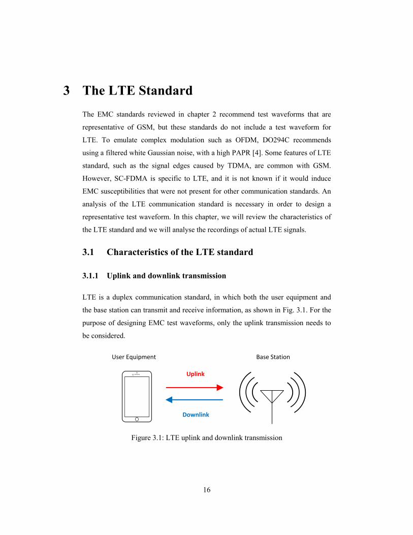
3.1 Characteristics of the LTE standard ...................................................... 16
3.1.1 Uplink and downlink transmission ......................................... 16
3.1.2 Frequency and time division duplexing .................................. 17
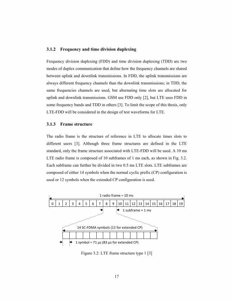
3.1.3 Frame structure ....................................................................... 17
3.1.4 Uplink physical channels ........................................................ 18
3.1.5 LTE frequency spectrum operating bands .............................. 18
3.1.6 Power control classes .............................................................. 19
3.1.7 Channel and transmission bandwidths .................................... 19
3.1.8 Sounding Reference Signal ..................................................... 20
3.1.9 Spectrum emission mask ......................................................... 21
3.1.10 Summary of LTE characteristics............................................. 21
3.2 Analysis of LTE signal recordings ....................................................... 22
3.2.1 LTE signal recording .............................................................. 22
3.2.2 Spectrum analysis ................................................................... 23
3.2.3 PAPR analysis ......................................................................... 27
3.2.4 Second LTE signal .................................................................. 28
3.2.5 Third LTE signal ..................................................................... 31
3.3 Summary ............................................................................................... 33
4 Test waveform design ..................................................................................... 34
4.1 Methodology and considerations .......................................................... 34
4.1.1 Parameter reduction process ................................................... 35
4.1.2 Spectrum emission mask adjustments ..................................... 36
4.2 LTE waveform design .......................................................................... 37
4.2.1 SystemVue signal generator for LTE ...................................... 37
4.2.2 Spectrum analysis of the LTE signals ..................................... 38
4.2.3 PAPR analysis of the LTE signals .......................................... 40
4.3 SC-FDMA waveform design ................................................................ 41
4.3.1 Spectrum analysis of the SC-FDMA signals .......................... 42
4.3.2 PAPR of the SC-FDMA signals.............................................. 44

viii
4.4 Filtered QPSK waveform design .......................................................... 45
4.4.1 RRC filter design .................................................................... 46
4.4.2 Spectrum of the filtered QPSK signals ................................... 47
4.4.3 PAPR of the filtered QPSK signals ......................................... 49
4.5 Filtered noise waveform design ............................................................ 50
4.5.1 Noise signals with a Gaussian probability distribution ........... 50
4.5.2 Noise signals with a uniform probability distribution ............. 52
4.5.3 PAPR of the noise signals ....................................................... 53
4.5.4 Spectrum of the noise signals .................................................. 54
4.6 Pulse modulated waveform design ....................................................... 56
4.6.1 SystemVue model for the pulse modulated signals ................ 56
4.6.2 Trapezoidal pulse model ......................................................... 57
4.6.3 Fourier series analysis ............................................................. 57
4.6.4 Spectrum of the pulse modulated signals ................................ 58
4.7 Choice of test waveforms parameters ................................................... 60
4.8 PAPR analysis and comparison ............................................................ 62
4.8.1 MCS index 1 and QPSK symbol mapping .............................. 62
4.8.2 MCS index 28 and 64-QAM symbol mapping ....................... 63
4.9 Summary ............................................................................................... 64
5 Radiated susceptibility testing ......................................................................... 65
5.1 Choice of victim system ....................................................................... 65
5.2 Radiated susceptibility testing setup ..................................................... 67
5.2.1 Vector signal generator setup ....................................................... 67
5.2.2 Antenna and DUT setup .......................................................... 68
5.2.3 Oscilloscope setup ....................................................................... 68
5.3 Interference induced by the test waveforms ......................................... 69
5.3.1 LTE waveforms ...................................................................... 69
5.3.2 SC-FDMA waveforms ............................................................ 71
5.3.3 Filtered QPSK waveforms ...................................................... 72
5.3.4 Filtered noise waveforms ........................................................ 73
5.3.5 Pulse modulated waveforms ................................................... 74
ix
5.3.6 Comparing the interference power measurements .................. 77
5.3.7 Sweeping carrier frequencies .................................................. 79
5.4 Summary ............................................................................................... 83
6 Conclusion ...................................................................................................... 84
6.1 Summary ............................................................................................... 84
6.2 Conclusions ........................................................................................... 84
6.3 Contributions ........................................................................................ 85
6.4 Future Work .......................................................................................... 85
Bibliography ........................................................................................................... 86
x
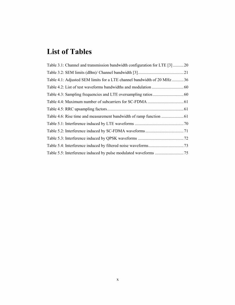
List of Tables
Table 3.1: Channel and transmission bandwidth configuration for LTE [3] .......... 20
Table 3.2: SEM limits (dBm)/ Channel bandwidth [3] ........................................... 21
Table 4.1: Adjusted SEM limits for a LTE channel bandwidth of 20 MHz ........... 36
Table 4.2: List of test waveforms bandwidths and modulation .............................. 60
Table 4.3: Sampling frequencies and LTE oversampling ratios ............................. 60
Table 4.4: Maximum number of subcarriers for SC-FDMA .................................. 61
Table 4.5: RRC upsampling factors ........................................................................ 61
Table 4.6: Rise time and measurement bandwidth of ramp function ..................... 61
Table 5.1: Interference induced by LTE waveforms .............................................. 70
Table 5.2: Interference induced by SC-FDMA waveforms .................................... 71
Table 5.3: Interference induced by QPSK waveforms ........................................... 72
Table 5.4: Interference induced by filtered noise waveforms ................................. 73
Table 5.5: Interference induced by pulse modulated waveforms ........................... 75
xi
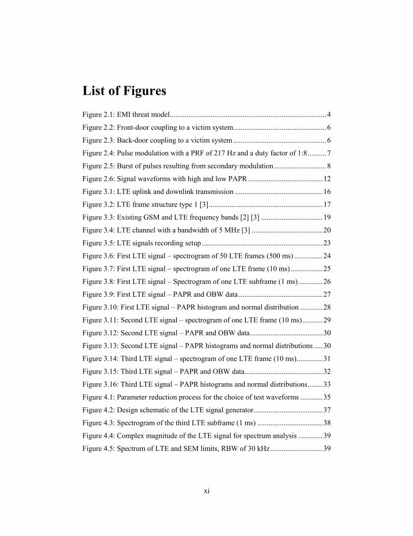
List of Figures
Figure 2.1: EMI threat model.................................................................................... 4
Figure 2.2: Front-door coupling to a victim system.................................................. 6
Figure 2.3: Back-door coupling to a victim system .................................................. 6
Figure 2.4: Pulse modulation with a PRF of 217 Hz and a duty factor of 1:8 .......... 7
Figure 2.5: Burst of pulses resulting from secondary modulation ............................ 8
Figure 2.6: Signal waveforms with high and low PAPR ........................................ 12
Figure 3.1: LTE uplink and downlink transmission ............................................... 16
Figure 3.2: LTE frame structure type 1 [3] ............................................................. 17
Figure 3.3: Existing GSM and LTE frequency bands [2] [3] ................................. 19
Figure 3.4: LTE channel with a bandwidth of 5 MHz [3] ...................................... 20
Figure 3.5: LTE signals recording setup ................................................................. 23
Figure 3.6: First LTE signal – spectrogram of 50 LTE frames (500 ms) ............... 24
Figure 3.7: First LTE signal – spectrogram of one LTE frame (10 ms) ................. 25
Figure 3.8: First LTE signal – Spectrogram of one LTE subframe (1 ms) ............. 26
Figure 3.9: First LTE signal – PAPR and OBW data ............................................. 27
Figure 3.10: First LTE signal – PAPR histogram and normal distribution ............ 28
Figure 3.11: Second LTE signal – spectrogram of one LTE frame (10 ms) ........... 29
Figure 3.12: Second LTE signal – PAPR and OBW data ....................................... 30
Figure 3.13: Second LTE signal – PAPR histograms and normal distributions ..... 30
Figure 3.14: Third LTE signal – spectrogram of one LTE frame (10 ms) .............. 31
Figure 3.15: Third LTE signal – PAPR and OBW data.......................................... 32
Figure 3.16: Third LTE signal – PAPR histograms and normal distributions ........ 33
Figure 4.1: Parameter reduction process for the choice of test waveforms ............ 35
Figure 4.2: Design schematic of the LTE signal generator ..................................... 37
Figure 4.3: Spectrogram of the third LTE subframe (1 ms) ................................... 38
Figure 4.4: Complex magnitude of the LTE signal for spectrum analysis ............. 39
Figure 4.5: Spectrum of LTE and SEM limits, RBW of 30 kHz ............................ 39
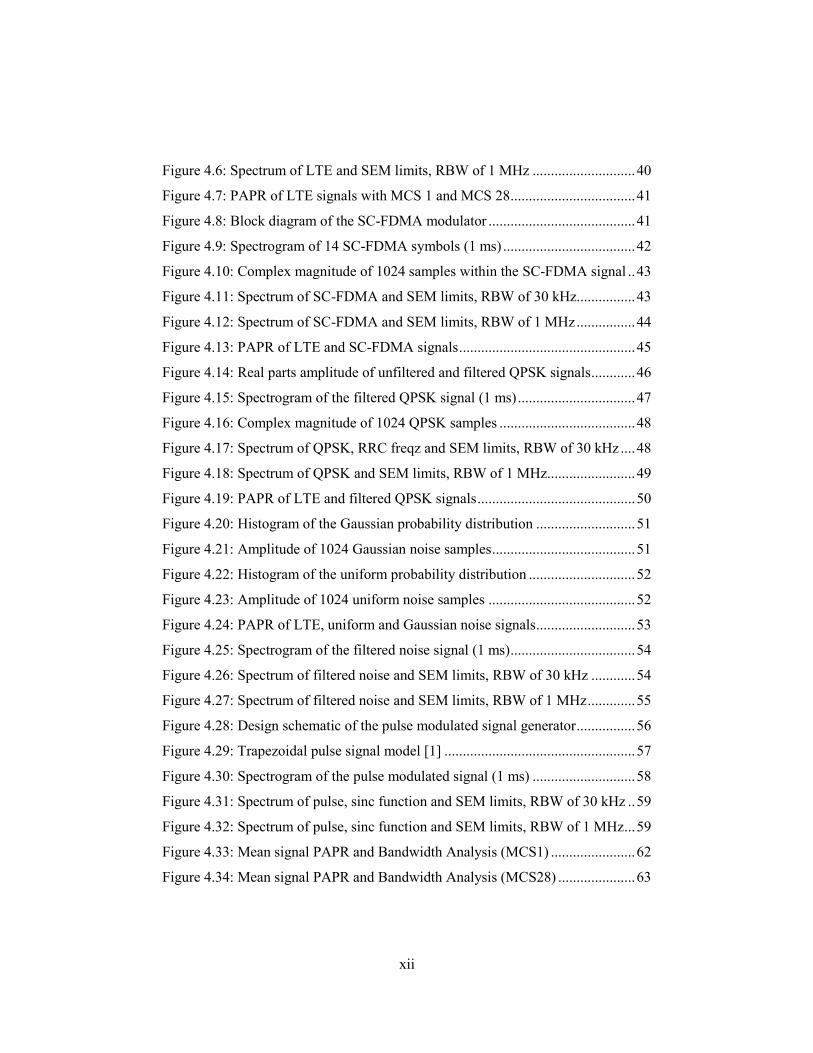
xii
Figure 4.6: Spectrum of LTE and SEM limits, RBW of 1 MHz ............................ 40
Figure 4.7: PAPR of LTE signals with MCS 1 and MCS 28 .................................. 41
Figure 4.8: Block diagram of the SC-FDMA modulator ........................................ 41
Figure 4.9: Spectrogram of 14 SC-FDMA symbols (1 ms) .................................... 42
Figure 4.10: Complex magnitude of 1024 samples within the SC-FDMA signal .. 43
Figure 4.11: Spectrum of SC-FDMA and SEM limits, RBW of 30 kHz................ 43
Figure 4.12: Spectrum of SC-FDMA and SEM limits, RBW of 1 MHz ................ 44
Figure 4.13: PAPR of LTE and SC-FDMA signals ................................................ 45
Figure 4.14: Real parts amplitude of unfiltered and filtered QPSK signals ............ 46
Figure 4.15: Spectrogram of the filtered QPSK signal (1 ms) ................................ 47
Figure 4.16: Complex magnitude of 1024 QPSK samples ..................................... 48
Figure 4.17: Spectrum of QPSK, RRC freqz and SEM limits, RBW of 30 kHz .... 48
Figure 4.18: Spectrum of QPSK and SEM limits, RBW of 1 MHz........................ 49
Figure 4.19: PAPR of LTE and filtered QPSK signals ........................................... 50
Figure 4.20: Histogram of the Gaussian probability distribution ........................... 51
Figure 4.21: Amplitude of 1024 Gaussian noise samples ....................................... 51
Figure 4.22: Histogram of the uniform probability distribution ............................. 52
Figure 4.23: Amplitude of 1024 uniform noise samples ........................................ 52
Figure 4.24: PAPR of LTE, uniform and Gaussian noise signals ........................... 53
Figure 4.25: Spectrogram of the filtered noise signal (1 ms) .................................. 54
Figure 4.26: Spectrum of filtered noise and SEM limits, RBW of 30 kHz ............ 54
Figure 4.27: Spectrum of filtered noise and SEM limits, RBW of 1 MHz ............. 55
Figure 4.28: Design schematic of the pulse modulated signal generator ................ 56
Figure 4.29: Trapezoidal pulse signal model [1] .................................................... 57
Figure 4.30: Spectrogram of the pulse modulated signal (1 ms) ............................ 58
Figure 4.31: Spectrum of pulse, sinc function and SEM limits, RBW of 30 kHz .. 59
Figure 4.32: Spectrum of pulse, sinc function and SEM limits, RBW of 1 MHz ... 59
Figure 4.33: Mean signal PAPR and Bandwidth Analysis (MCS1) ....................... 62
Figure 4.34: Mean signal PAPR and Bandwidth Analysis (MCS28) ..................... 63
xiii
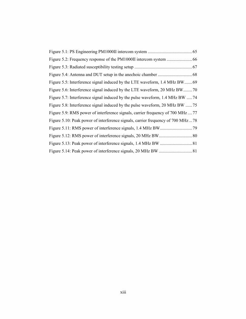
Figure 5.1: PS Engineering PM1000II intercom system ........................................ 65
Figure 5.2: Frequency response of the PM1000II intercom system ....................... 66
Figure 5.3: Radiated susceptibility testing setup .................................................... 67
Figure 5.4: Antenna and DUT setup in the anechoic chamber ............................... 68
Figure 5.5: Interference signal induced by the LTE waveform, 1.4 MHz BW ....... 69
Figure 5.6: Interference signal induced by the LTE waveform, 20 MHz BW ........ 70
Figure 5.7: Interference signal induced by the pulse waveform, 1.4 MHz BW ..... 74
Figure 5.8: Interference signal induced by the pulse waveform, 20 MHz BW ...... 75
Figure 5.9: RMS power of interference signals, carrier frequency of 700 MHz .... 77
Figure 5.10: Peak power of interference signals, carrier frequency of 700 MHz ... 78
Figure 5.11: RMS power of interference signals, 1.4 MHz BW............................. 79
Figure 5.12: RMS power of interference signals, 20 MHz BW.............................. 80
Figure 5.13: Peak power of interference signals, 1.4 MHz BW ............................. 81
Figure 5.14: Peak power of interference signals, 20 MHz BW .............................. 81
xiv
List of Acronyms
CCDF Complementary Cumulative Distribution Function
CSV Comma-Separated Values
DMRS Demodulation Reference Signals
DoD United States Department of Defense
DTx Discontinuous Transmission
DUT Device Under Test
EMC Electromagnetic Compatibility
EMI Electromagnetic Interference
FCC Federal Communications Commission
FDD Frequency Division Duplexing
FDMA Frequency Division Multiple Access
GMSK Gaussian Minimum Shift Keying
GSM Global System for Mobile communications
HIRF High Intensity Radiated Fields
IBS Isotropic Broadband Susceptibility
IEC International Electrotechnical Commission
LTE Long Term Evolution
MCS Modulation Coding Scheme
OBW Occupied Bandwidth
OFDM Orthogonal Frequency Division Multiplexing
PAPR Peak to Average Power Ratio
PDF Probability Density Function
PED Portable Electronic Devices
PRACH Physical Random Access Channel
PRF Pulse Repetition Frequency
PSD Power Spectral Density
PUCCH Physical Uplink Control Channel
xv
PUSCH Physical Uplink Shared Channel
QAM Quadrature Amplitude Modulation
QPSK Quadrature Phase Shift Keying
RBW Resolution Bandwidth
RRC Root Raised Cosine
RTCA Radio Technical Commission for Aeronautics
SC-FDMA Single Carrier FDMA
SEM Spectrum Emission Mask
SRS Sounding Reference Signal
TDD Time Division Duplexing
TDMA Time Division Multiple Access
UMTS Universal Mobile Telecommunications System
VSA Vector Signal Analyzer
VSG Vector Signal Generators
W-CDMA Wideband Code Division Multiple Access
1
1 Introduction
1.1 Background
Portable Electronic Devices (PEDs) such as mobile phones and portable computers
are replacing paper publications in the aircraft cabin. These devices, known as
electronic flight bags, are routinely used by the crew. By their nature, PEDs
transmit electromagnetic radiation in the form of intentional and non-intentional
emissions. These emissions pose a risk Electromagnetic Interference (EMI): they
can disturb the normal function of the avionic systems, which can lead to
disastrous consequences if the affected systems are flight safety-critical.
Allowing the use of PEDs in the aircraft cockpit environment is an old issue:
the Radio Technical Commission for Aeronautics (RTCA), a private not-for-profit
organization, has been studying the problem for over 30 years. To simplify the
EMI analysis, the interference coupling path between the source and the victim are
categorized in two types: front-door coupling, and back-door coupling. Front-door
coupling is the transmission of electromagnetic energy through an entry that was
designed to receive a signal during normal operation; back-door coupling is the
transmission of energy through an entry of which the function is not to receive a
signal. In this thesis, only the back-door coupling interference will be studied.
To allow the use of PEDs in the aircraft cabin environment, aviation authorities
must ensure the immunity of the avionic systems to the different types of EMI.
Back-door immunity to intentional PED emissions can be verified by radiated
susceptibility testing: a signal is transmitted in proximity to an avionic system, and
the response of the system is monitored to detect any disturbance.
RTCA document 294C proposed a list of test waveforms to emulate the
communications standards that were current when the document was published in
2008 [4]. Such waveforms were recommended for use in radiated susceptibility
2
testing, to ensure that the avionic systems were not affected by communication
signals that could be emitted by the PEDs.
The most recent recommendations by the RTCA mark a departure from
previous guidance. RTCA document 307A recommended the use of a continuous
signal for radiated susceptibility testing; similar to the signal used for high intensity
radiated fields (HIRF) testing [5]. It argued that existing HIRF protection could
provide some immunity to PED emissions. It proposed that the waveforms from
document 294C can be used for additional testing; however the test waveforms
were not updated to include the most recent communication standards.
1.2 Problem Statement
The aeronautical industry is motivated in allowing the use of PEDs inside the
aircraft cabin to replace paper publications. However, testing for EMI immunity to
complex communication standards is challenging. With the advent of vector signal
generators, there is an interest for the use of complex waveforms that are closer to
the real interfering signal. Test waveforms must have enough simplicity to ensure
their repeatability, and reduce the testing time to a minimum. Few publications are
available on the subject of EMI susceptibility to intentional radiated emissions with
back-door coupling. Finally, there is no consensus in the Electromagnetic
Compatibility (EMC) industry standards or in published literature on the type of
waveforms that can be used to simulate the interference effects of the Long Term
Evolution (LTE) communication standard.
1.3 Thesis Statement
EMI immunity to complex communication standards such as LTE can be tested
using waveforms with reduced parameters. The objective of this research is to
develop waveforms that are representative of the LTE communication standard,
with enough simplicity for practical use in radiated susceptibility testing.
3
1.4 Methodology
In order to design test waveforms that are representative of LTE, it is necessary
that they share the same signal properties. The first step of this thesis is to study the
LTE communication standard: the characteristics of LTE that are suspected to have
an effect on the back-door interference will be described, and LTE signals will be
analyzed. Second, the waveforms that will be used in radiated susceptibility testing
will be developed: a parameters reduction process will used to obtain test
waveforms with properties that are similar to LTE waveforms. Third, radiated
susceptibility testing will determine if the test waveforms are valid waveforms for
use in EMI testing of the LTE standard.
1.5 Thesis Outline
Chapter 2 will survey the current EMC standards to compare the recommended test
waveforms, and review the state of research on radiated susceptibility testing.
Chapter 3 will provide a summary of the LTE standard, with the properties that
make it different from other communication standards. The occupied bandwidths
and the peak to average power ratio will be measured in LTE signal recordings.
Chapter 4 will explain the design of test waveforms. LTE, SC-FDMA, QPSK,
noise, and pulse modulated signals will be developed in accordance with the
spectrum emission mask of LTE, for five different channel bandwidths. Chapter 5
will cover the radiated susceptibility testing with the waveforms. An avionic
system will be chosen to become the device under test. The RMS and the peak
power of the interference induced by the different waveforms will be measured for
multiple carrier frequencies. The radiated test results will be analyzed to determine
the validity of the test waveforms. Chapter 6 will conclude this thesis, and will
propose future research work on the subject of radiated susceptibility testing.
4
2 Literature survey
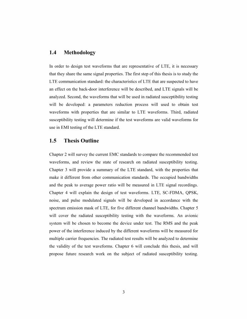
The most basic decomposition of any EMI problem has three elements: an emitter,
a coupling path, and a receiver [1]. In the context of this research, the mobile
device is the emission source, and any aircraft electronic system can become a
receiver. The coupling path is the transfer of electromagnetic energy though the
aircraft environment, as shown in Fig. 2.1. In this chapter, different aspects of the
source, the coupling path, and the receiver will be studied.
Figure 2.1: EMI threat model
2.1 Commercial Mobile Communication Emission sources
Personal electronic devices (PEDs) are required to adhere to standards for their
emissions. In the USA, the Federal Communications Commission (FCC) regulates
electromagnetic radiation from electronic devices, restricting the field strength of
emissions radiated within specified frequency bands. In Canada, the Spectrum
Management branch of Innovation, Science and Economic Development Canada
(previously Industry Canada) specifies the emission limits in certification
requirements for electronic devices. Although modern PEDs can use various
wireless protocols, including Bluetooth and Wi-Fi, we will restrict our attention to
two mobile telephony standards only, namely the Global System for Mobile
communications (GSM) and Long Term Evolution (LTE).
Emission Source Coupling Path Receiver
5
2.1.1 The Global System for Mobile Communications (GSM)
The GSM communication standard is a second generation (2G) mobile
telecommunications technology [2]. GSM uses time division multiple access
(TDMA), in which time slots are allocated to different users on the same frequency
channels. The GSM frame structure is composed of TDMA frames with a length of
4.6 ms. GSM uses a separation of 200 kHz between each frequency channel, with a
frequency hopping sequence to reduce interference between adjacent channels.
GSM uses Gaussian Minimum Shift Keying (GMSK) modulation: the data is
modulated on the carrier signal by changing the phase of the carrier.
An important aspect of GSM is its discontinuous transmission (DTx). DTx is a
state where bursts can only be transmitted during specific TDMA frames to reduce
power consumption of the mobile device when continuous voice transmission is
not required. DTx also helps to reduce interference between GSM devices.
2.1.2 Long Term Evolution (LTE)
The Long Term Evolution (LTE) communication standard is a fourth generation
(4G) mobile telecommunications technology [3]. LTE uses TDMA, but also
frequency division multiple access (FDMA): specific time slots and frequencies
within a channel are allocated to different users.
LTE uses the single carrier FDMA (SC-FDMA) to transmit data in uplink
channels. SC-FDMA is similar to the orthogonal frequency division multiplexing
(OFDM) used in Wi-Fi, in that the channel bandwidth is mapped into subcarriers.
Chapter 3 will discuss the important characteristics of the LTE communication
standard in further detail.
6
2.2 Interference coupling paths
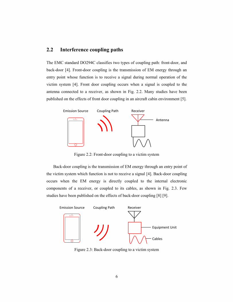
The EMC standard DO294C classifies two types of coupling path: front-door, and
back-door [4]. Front-door coupling is the transmission of EM energy through an
entry point whose function is to receive a signal during normal operation of the
victim system [4]. Front door coupling occurs when a signal is coupled to the
antenna connected to a receiver, as shown in Fig. 2.2. Many studies have been
published on the effects of front door coupling in an aircraft cabin environment [5].
Figure 2.2: Front-door coupling to a victim system
Back-door coupling is the transmission of EM energy through an entry point of
the victim system which function is not to receive a signal [4]. Back-door coupling
occurs when the EM energy is directly coupled to the internal electronic
components of a receiver, or coupled to its cables, as shown in Fig. 2.3. Few
studies have been published on the effects of back-door coupling [8] [9].
Figure 2.3: Back-door coupling to a victim system
Antenna
Emission Source
Emission Source
Coupling Path
Coupling Path
Receiver
Receiver
Equipment Unit
Cables
7
2.3 EMC Standards
EMC standards provide guidance on the emission and susceptibility tests necessary
to certify a product’s conformance. Publications from three EMC standards
organizations were reviewed for the purpose of this project: the Radio Technical
Commission for Aeronautics (RTCA), the International Electrotechnical
Commission (IEC), and the United States Department of Defense (DoD). Each of
these organizations has a different vision in the development of EMC standards,
and they recommend different waveforms for EMI susceptibility testing.
2.3.1 Radio Technical Commission for Aeronautics (RTCA)
The RTCA’s role is to offer technical recommendations to civil aviation authorities
and to the aerospace industry. DO294C provides a framework for the
characterization of PEDs: it describes coupling paths in an aircraft configuration,
and it sets EMI susceptibility levels for aircraft systems [4].
For the purpose of EMI susceptibility testing of aircraft systems, DO294C
proposes a list of test waveforms corresponding to specific communication
standards. Two types of waveforms are proposed: pulse modulated waveforms, and
continuous waveforms. To emulate a communication standard using TDMA such
as GSM, DO294C recommends a pulse modulated signal, with a pulse repetition
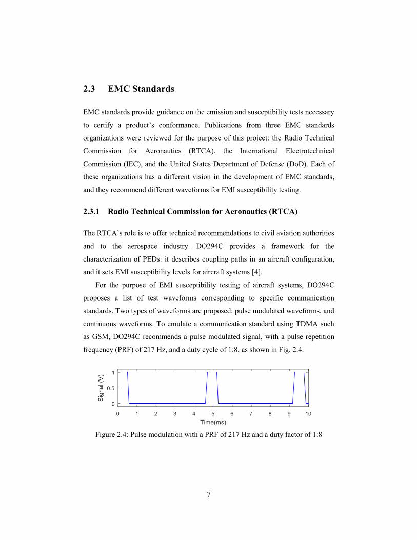
frequency (PRF) of 217 Hz, and a duty cycle of 1:8, as shown in Fig. 2.4.
Figure 2.4: Pulse modulation with a PRF of 217 Hz and a duty factor of 1:8
8
DO294C claims that phase modulation such as GMSK can be modeled by a
continuous wave, and that the effect of the peak signal power is more significant
than the effect of the signal energy. DO294C recommends the derivation of
extended waveforms for additional susceptibility testing. To emulate a PED using a
communication standard with complex modulation such as OFDM used in Wi-Fi,
DO294C recommends using a filtered white Gaussian noise, with a high peak to
average power ratio (PAPR).
2.3.2 International Electrotechnical Commission (IEC)
The IEC publishes international standards for electrical, electronic and related
technologies. IEC 61000-4-3 is a standard for radiated immunity testing and
measurements techniques [6]. It proposes three modulation methods for radiated
susceptibility testing. The first method is a sine wave amplitude modulation with a
frequency of 1 kHz and a modulation depth of 80%. The second method is a square
wave modulation with a PRF of 200 Hz, and a duty cycle of 1:2. The third method
is a pulse modulation with a duty cycle and a PRF that correspond to a specific
communication standard. For GSM, 61000-4-3 recommends a pulse modulation
with a PRF of 217 Hz and, a duty cycle of 1:8, similar to DO294C.
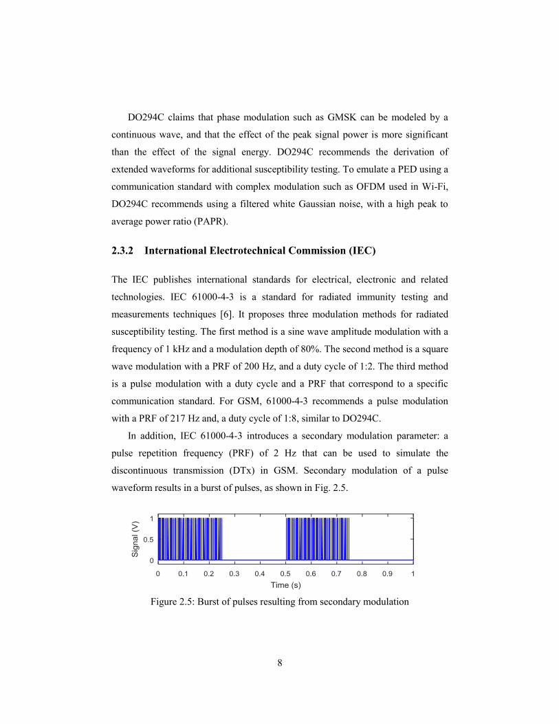
In addition, IEC 61000-4-3 introduces a secondary modulation parameter: a
pulse repetition frequency (PRF) of 2 Hz that can be used to simulate the
discontinuous transmission (DTx) in GSM. Secondary modulation of a pulse
waveform results in a burst of pulses, as shown in Fig. 2.5.
Figure 2.5: Burst of pulses resulting from secondary modulation
9
2.3.3 United States Department of Defense (DoD)
MIL-STD-461 is a standard published by the DoD to establish EMI emission and
susceptibility requirements for equipment designed or purchased by the DoD [7].
The requirements for radiated susceptibility to the electric field are outlined in
section RS103 of MIL-STD-461: aircraft safety critical equipment must be tested
to electric field strengths of 200 V/m for frequencies from 2 MHz to 40 GHz.
Other aircraft equipment must be tested to 20 V/m from 2 MHz to 1 GHz, and to
electric field strengths of 60 V/m for frequencies from 1 GHz to 40 GHz.
MIL-STD-461 indicates that the susceptibility test signals shall be a pulse
modulated signal with a PRF of 1 kHz and a duty cycle of 50%. The reason for the
choice of a PRF 1 kHz is because it normally falls within the range of frequencies
that can pass through audio and video filters of certain subsystems with a low
frequency response characteristic, such as aircraft flight control subsystems.
2.3.4 Comparison of radiated susceptibility waveforms
All three EMC standard organizations recommended the use of a pulse modulated
waveform to test for the radiated susceptibility of communications standards with
TDMA. RTCA DO294C and IEC 61000-4-3 provided the same waveform
parameters to emulate the GSM: a PRF of 217 Hz and a duty cycle of 1:8. The
pulse modulated waveform can easily be reproduced in a testing environment.
However, no recommendations were given on the pulse’s rise time when testing for
radiated susceptibility. A faster rise time could increase the frequency content of
the pulse modulated waveform, and could have an effect on the victim systems.
None of the EMC standards provided a test waveform for the LTE
communication standard. DO294C recommends the use of filtered white Gaussian
noise to emulate OFDM signals; neither the IEC 61000-4-3 nor the MIL-STD-461
proposed additional waveforms to emulate complex communication standards. The
existing waveforms are simple, but not representative of the signals used in LTE.
10
2.4 Radiated susceptibility studies
Several radiated susceptibility studies were reviewed for the purpose of this thesis.
However, few studies were relevant to the derivation of waveforms for radiated
susceptibility testing in an aircraft cockpit environment. In this section, four
research publications on the study of test waveforms for radiated susceptibility will
be presented. These studies provided a starting point for the design of test
waveforms to be used in the context of radiated susceptibility to the LTE standard.
2.4.1 Isotropic Broadband Susceptibility (IBS) method
A study performed at the Naval Air Warfare Center compared the Isotropic
Broadband Susceptibility (IBS) method to the RS103 method for EMI testing with
back-door coupling [8]. The IBS method uses a band limited white Gaussian noise,
such as described in DO294C. White Gaussian noise has the particularity of
spreading the power over a large frequency band, and filtering the white Gaussian
noise limits the frequency bandwidth of the signal. The IBS method was performed
in a mode-stirred reverberating chamber: it has the advantage of illuminating the
victim from all directions.
The RS103 method uses a pulse modulated signal, as described in section 2.4.3
[7]. It has a significantly lower frequency than the band limited white Gaussian
noise. The RS103 method is typically performed in an anechoic chamber: multiple
changes of antenna positions are required to illuminate the equipment under test.
The ARC-182 VHF/UHF Radio Receiver was chosen as a victim system for its
narrow failure bandwidth, and the receiver was tested with both methods [8]. The
IBS method was tested with noise bandwidths of 1.6, 6, 12, 22, and 56 MHz. The
test was repeated with different carrier frequencies. Susceptibility thresholds were
measured as the lowest electric field strength that caused a failure of the receiver.
The IBS method discovered a susceptibility at 663 MHz that was not found during
11
the RS103 test. The susceptibility thresholds of the IBS method were higher than
the susceptibility thresholds of RS103: higher field strengths were required for the
IBS method than for RS103 to induce the same level of interference.
The author concluded that the IBS method could be used to replace RS103,
because the susceptibilities found with RS103 were also found with the IBS
method. The IBS method is also faster than for the RS103 method: fewer carrier
frequency increments are required to cover the test frequencies, and fewer changes
in the antenna positions are required to illuminate the equipment under test.
The main disadvantage of the IBS method is that the signal is difficult to
reproduce with accuracy: the signals’ frequency bandwidth was the only known
characteristic of the noise generator. More research is required to establish the
susceptibility thresholds associated with the IBS method. Vector signal generators
could be used to transmit a signal that can be reproduced with higher accuracy.
2.4.2 Effect of modulated signal rise time
As discussed in section 2.3.4, the EMC standards did not provide recommendations
on the modulated signal’s rise time when testing for radiated susceptibility. To
address this deficiency, a study performed at the NASA Langley Research Center
evaluated the effects of the rise time [9]. The susceptibility thresholds relative were
measured for three modulated signals: a square wave with a rise time of 630 ns, a
square wave with a rise time of 14 ns, and a 1 µs pulse modulated signal with a rise
time of 14 ns.
The signal with a rise time of 630 ns had higher susceptibility thresholds than
both signals with a rise time of 14 ns: higher field strengths were required to induce
the same level of interference. The authors concluded that the modulation rise time
had a significant effect on EMI susceptibility. However, in order to design pulse
waveforms for radiated susceptibility, it would be necessary to determine the rise
times that are representative of specific communication standards.
12
2.4.3 Effect of the Peak to Average Power Ratio (PAPR)
A study performed at NTT DoCoMo research laboratories, Japan, evaluated the
effect of the peak to average power ratio (PAPR) on medical devices [10]. PAPR,
also known as crest factor or peak-to-average ratio, is a measure of the relative
peak power of a signal, as expressed in (1.1)
[ ] [ ] [ ] (1.1)
where is the peak power, and is the average power, expressed in decibels.
A representation of signal waveforms with a high and low PAPR is shown in
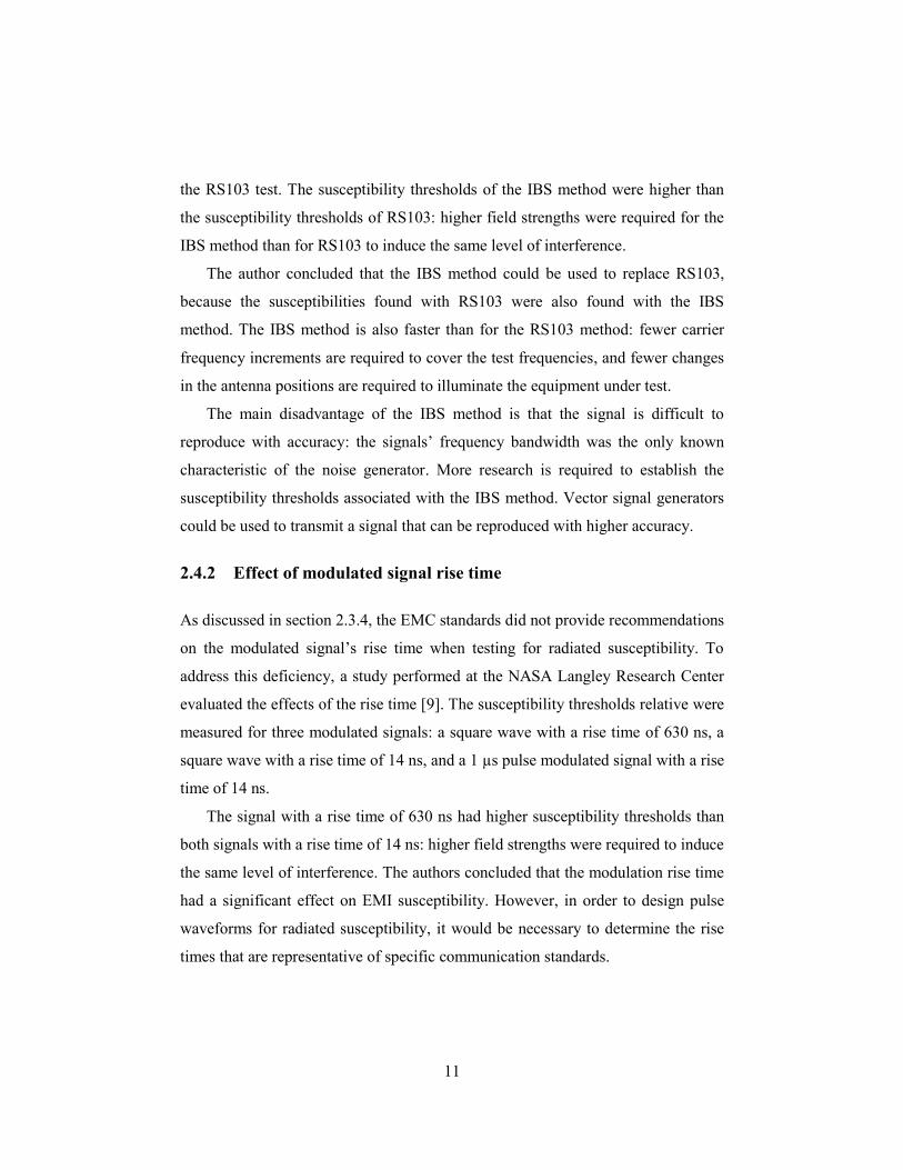
Fig. 2.6. Multicarrier modulation, such as SC-FDMA used in LTE standard, yields
a higher PAPR than phase modulation, such as GMSK used in the GSM standard.
Figure 2.6: Signal waveforms with high and low PAPR
The authors compared the EMI effects of LTE and Wideband Code Division
Multiple Access (W-CDMA) signals [10]. W-CDMA is a third generation (3G)
mobile telecommunication technology, based on CDMA, a channel access method
where specific codes are allocated to different users. CDMA is a spread spectrum
technology, for the signal is spread on a large frequency bandwidth.
Two different releases of W-CDMA were used in this study: release 99, also
known as the Universal Mobile Telecommunications System (UMTS), and release
6, also known as High Speed Packet Access (HSPA). W-CDMA release 99 and
release 6 signals had PAPR values of 3.6 dB and 5.1 dB, respectively.
RMS
t
(t) (t)
RMS
Max
Max
Low PAPR signal High PAPR signal
13
LTE release 8 signals were used, which had a PAPR of 7.7 dB. The PAPR
values were for a complementary cumulative distribution function (CCDF)
probability of 0.0001%: the PAPR was computed using one million samples.
The authors measured the maximum distance at which an EMI effect was
observed [10]. The measurements were repeated for the three test signals using two
transmitted power levels: a typical transmission power (10 dBm), and the
maximum transmission power (23 or 24 dBm). Two carrier frequency bands were
chosen to take the measurements: 2 GHz, and 800 MHz.
The authors found that the change in PAPR had no significant effect to the
EMI disappearing distance, except for one case: using peak transmission power at
800 MHz, the W-CDMA release 6 signals had a slightly larger disappearing
distance than the release 99 signals. All other signals had approximately the same
EMI disappearing distance, independently of the peak transmission power.
These findings disagree with DO294C’s suggestion that the peak signal power
has a significant effect on the susceptibility. In order to determine the effect of
PAPR, it would be necessary to perform additional radiation susceptibility testing
with different PAPR values, while controlling the other parameters.
2.4.4 Effect of the discontinuous transmission mode
Another study performed at NTT Network Technology laboratories evaluated the
effects of the discontinuous transmission mode on the interference to 32 different
medical devices [11]. Similar to the previous study, the authors measured the EMI
disappearing distance of three communication standards: the LTE, HSPA, and the
Wideband Code Division Multiple Access (W-CDMA).
Two different transmission modes were chosen for susceptibility testing: a
discontinuous mode, and a continuous mode. The discontinuous transmission mode
had a pulse repetition interval of 1 s and a duty cycle of 50%. The pulse repetition
interval was chosen to increase the susceptibility of medical devices used to detect
14
biological rhythms such as breathing and the heartbeat. The authors expected that
discontinuous transmission mode would lead to induce higher levels of EMI [11].
Discontinuous waveforms were used to perform radiated susceptibility testing
on all medical devices: 12 of the 32 medical devices were affected by the
discontinuous transmissions. Then, the continuous waveforms were used to test
only the medical devices for which EMI occurred in the discontinuous tests: 7 of
the 12 medical devices tested were also affected by the continuous transmission.
The maximum EMI disappearing distance was 80 cm for the discontinuous
transmission, compared to 28 cm for the continuous transmission. The authors
concluded that the discontinuous transmission mode could induce higher levels of
interference to medical devices than the continuous transmission mode.
The authors did not use any of the test waveforms that are recommended by the
EMC standards as a point of comparison to evaluate the radiated susceptibility of
the medical devices. It is suspected that the discontinuous transmission mode can
be emulated with a pulse modulated waveform; however this hypothesis cannot be
validated without actual susceptibility measurement. Moreover, the authors gave
no indication on the transition time between the transmitters on and off states.
2.4.5 Effect of the Orthogonal Frequency Division Multiplexing
A study performed at NTT Network Technology laboratories, Japan, evaluated the
effect of the Orthogonal Frequency Division Multiplexing (OFDM) modulation for
back-door radiated immunity tests in close proximity to equipment [12]. The effect
of OFDM modulation was compared to pulse modulation (217 Hz, 50% duty
cycle) and amplitude modulation (1 kHz, 80% depth). The OFDM signal had a
discontinuous temporal waveform to emulate the IEEE 802.11 communication
standard (Wi-Fi). The authors used two different test setups to perform the radiated
immunity measurements. The first setup used a gigahertz transverse
electromagnetic cell to expose the device under test (DUT) to an electric field with
15
gradually increasing field strength. The immunity levels were defined as the lowest
field strengths which caused errors. The immunity levels were measured for the
OFDM, pulse, and amplitude modulated signals. The immunity levels of the
OFDM signal were found to be closer to the levels of the pulse modulated signal
than the levels of the amplitude modulated signals.
The second setup used a double-ridged horn antenna. The antenna was
positioned at a distance of 100 mm from the EUT. Because the size of the uniform
electric field plane (20 cm x 8 cm) was smaller than the dimensions of the DUT,
the surface of the DUT was divided into four areas. Measurements were taken with
the antenna aligned on the center of each area. OFDM, pulse, and amplitude
modulated signals were used to illuminate the DUT. In the first area, the immunity
levels of the OFDM signal were significantly lower than the immunity levels of the
pulse and amplitude modulated signals. In the three other areas, the immunity
levels of the amplitude modulated signal were found to be almost always lower
than the immunity levels of the OFDM signal and the pulse modulated signal. The
authors concluded that the test method for radiated immunity testing should
consider using a wideband signal such as an OFDM modulated signal, in addition
to pulse and amplitude modulated signals.
2.5 Summary
Test waveforms from current EMC standards were found to be based on a pulse
modulated signal, with parameters representative of the GSM standard. However,
studies on radiated susceptibility showed that test waveforms with increased
complexity, such as Gaussian noise and OFDM signals yield different
susceptibility thresholds. Parameters, such as the rise time, the PAPR, and the
discontinuous transmissions were found to have a significant effect on EMI
immunity. Furthermore, few studies have provided considerations for the design of
test waveforms that are representative of the LTE standard.
16
3 The LTE Standard
The EMC standards reviewed in chapter 2 recommend test waveforms that are
representative of GSM, but these standards do not include a test waveform for
LTE. To emulate complex modulation such as OFDM, DO294C recommends
using a filtered white Gaussian noise, with a high PAPR [4]. Some features of LTE
standard, such as the signal edges caused by TDMA, are common with GSM.
However, SC-FDMA is specific to LTE, and it is not known if it would induce
EMC susceptibilities that were not present for other communication standards. An
analysis of the LTE communication standard is necessary in order to design a
representative test waveform. In this chapter, we will review the characteristics of
the LTE standard and we will analyse the recordings of actual LTE signals.
3.1 Characteristics of the LTE standard
3.1.1 Uplink and downlink transmission
LTE is a duplex communication standard, in which both the user equipment and
the base station can transmit and receive information, as shown in Fig. 3.1. For the
purpose of designing EMC test waveforms, only the uplink transmission needs to
be considered.
Figure 3.1: LTE uplink and downlink transmission
User Equipment Base Station
Uplink
Downlink
17
3.1.2 Frequency and time division duplexing
Frequency division duplexing (FDD) and time division duplexing (TDD) are two
modes of duplex communication that define how the frequency channels are shared
between uplink and downlink transmissions. In FDD, the uplink transmissions are
always different frequency channels than the downlink transmissions; in TDD, the
same frequencies channels are used, but alternating time slots are allocated for
uplink and downlink transmissions. GSM use FDD only [2], but LTE uses FDD in
some frequency bands and TDD in others [3]. To limit the scope of this thesis, only
LTE-FDD will be considered in the design of test waveforms for LTE.
3.1.3 Frame structure
The radio frame is the structure of reference in LTE to allocate times slots to
different users [3]. Although three frame structures are defined in the LTE
standard, only the frame structure associated with LTE-FDD will be used. A 10 ms
LTE radio frame is composed of 10 subframes of 1 ms each, as shown in Fig. 3.2.
Each subframe can further be divided in two 0.5 ms LTE slots. LTE subframes are
composed of either 14 symbols when the normal cyclic prefix (CP) configuration is
used or 12 symbols when the extended CP configuration is used.
Figure 3.2: LTE frame structure type 1 [3]
0
1 subframe = 1 ms
1 radio frame = 10 ms
14 SC-FDMA symbols (12 for extended CP)
1 symbol = 71 µs (83 µs for extended CP)
1 2 3 4 5 6 7 8 9 10 11 12 13 14 15 16 17 18 19
18
3.1.4 Uplink physical channels
The LTE standard uses three different uplink physical channels to carry
information blocks from the user equipment to the base station [3]:
1) The Physical Uplink Shared Channel (PUSCH): it is a transport channel
used to transmit the user data. It also carries the channel quality indicator and the
rank indicator to report the condition of the downlink channel to the base station.
2) Physical Uplink Control Channel (PUCCH): it is a logical channel used to
transmit uplink control information. It is transmitted simultaneously with PUSCH.
3) Physical Random Access Channel (PRACH): it is a transport channel used
by user equipment to access the LTE network for transmission set-up.
The PUCCH and the PRACH do not transmit user data. The transmission
length of these physical channels is typically shorter than the PUSCH’s: in the LTE
recordings analyzed in this chapter, the PUSCH occupied significantly more
transmission time than the PUCCH and the PRACH. Moreover, the transitions of
power in PUCCH and PRACH were similar to those of the PUSCH. For these
reasons, only the PUSCH will be used in the design of test waveforms.
Three modulations are available for the SC-FDMA symbols in the PUSCH:
quadrature phase shift keying (QPSK), 16 point quadrature amplitude modulation
(16QAM), and 64 point quadrature amplitude modulation (64QAM). The
modulation is determined by the modulation coding scheme (MCS) index, an
integer with a value interval from 0 to 28.
3.1.5 LTE frequency spectrum operating bands
The LTE standard uses a variety of frequency operating bands in order to adapt to
the spectrum allocation for mobile communication in different countries [3]. LTE
uses frequencies bands allocated for the GSM standard [2], with additional
frequencies bands that have been allocated for mobile communications since GSM
was introduced. Existing GSM and LTE frequency bands are shown in Fig. 3.3.
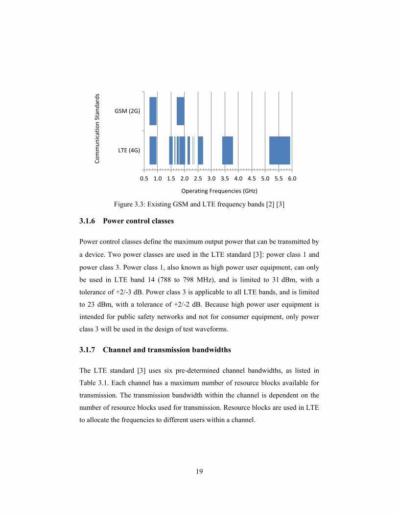
19
Figure 3.3: Existing GSM and LTE frequency bands [2] [3]
3.1.6 Power control classes
Power control classes define the maximum output power that can be transmitted by
a device. Two power classes are used in the LTE standard [3]: power class 1 and
power class 3. Power class 1, also known as high power user equipment, can only
be used in LTE band 14 (788 to 798 MHz), and is limited to 31 dBm, with a
tolerance of +2/-3 dB. Power class 3 is applicable to all LTE bands, and is limited
to 23 dBm, with a tolerance of +2/-2 dB. Because high power user equipment is
intended for public safety networks and not for consumer equipment, only power
class 3 will be used in the design of test waveforms.
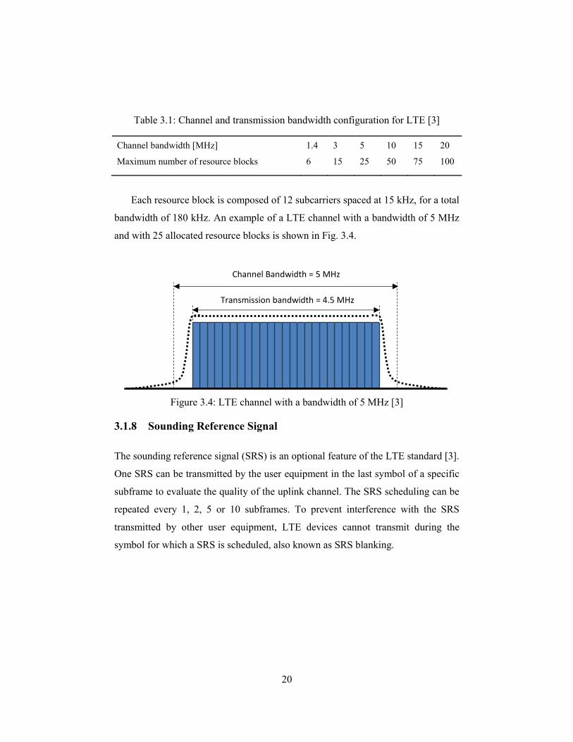
3.1.7 Channel and transmission bandwidths
The LTE standard [3] uses six pre-determined channel bandwidths, as listed in
Table 3.1. Each channel has a maximum number of resource blocks available for
transmission. The transmission bandwidth within the channel is dependent on the
number of resource blocks used for transmission. Resource blocks are used in LTE
to allocate the frequencies to different users within a channel.
0.5 1.0 1.5 2.0 2.5 3.0 3.5 4.0 4.5 5.0 5.5 6.0
LTE (4G)
GSM (2G)
Operating Frequencies (GHz)
Co
mm
un
icat
ion
Sta
nd
ard
s
20
Table 3.1: Channel and transmission bandwidth configuration for LTE [3]
Channel bandwidth [MHz]
Maximum number of resource blocks
1.4
6
3
15
5
25
10
50
15
75
20
100
Each resource block is composed of 12 subcarriers spaced at 15 kHz, for a total
bandwidth of 180 kHz. An example of a LTE channel with a bandwidth of 5 MHz
and with 25 allocated resource blocks is shown in Fig. 3.4.
Figure 3.4: LTE channel with a bandwidth of 5 MHz [3]
3.1.8 Sounding Reference Signal
The sounding reference signal (SRS) is an optional feature of the LTE standard [3].
One SRS can be transmitted by the user equipment in the last symbol of a specific
subframe to evaluate the quality of the uplink channel. The SRS scheduling can be
repeated every 1, 2, 5 or 10 subframes. To prevent interference with the SRS
transmitted by other user equipment, LTE devices cannot transmit during the
symbol for which a SRS is scheduled, also known as SRS blanking.
Channel Bandwidth = 5 MHz
Transmission bandwidth = 4.5 MHz
21
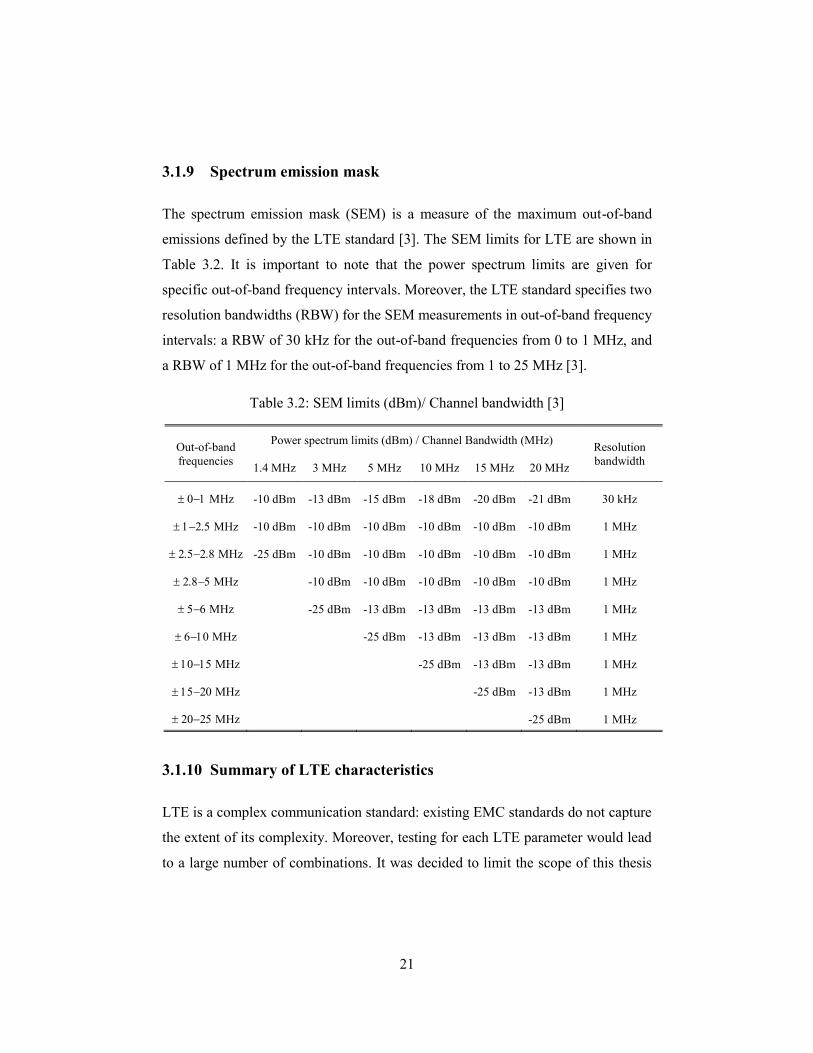
3.1.9 Spectrum emission mask
The spectrum emission mask (SEM) is a measure of the maximum out-of-band
emissions defined by the LTE standard [3]. The SEM limits for LTE are shown in
Table 3.2. It is important to note that the power spectrum limits are given for
specific out-of-band frequency intervals. Moreover, the LTE standard specifies two
resolution bandwidths (RBW) for the SEM measurements in out-of-band frequency
intervals: a RBW of 30 kHz for the out-of-band frequencies from 0 to 1 MHz, and
a RBW of 1 MHz for the out-of-band frequencies from 1 to 25 MHz [3].
Table 3.2: SEM limits (dBm)/ Channel bandwidth [3]
Out-of-band
frequencies
Power spectrum limits (dBm) / Channel Bandwidth (MHz) Resolution
bandwidth 1.4 MHz 3 MHz 5 MHz 10 MHz 15 MHz 20 MHz
MHz -10 dBm -13 dBm -15 dBm -18 dBm -20 dBm -21 dBm 30 kHz
MHz -10 dBm -10 dBm -10 dBm -10 dBm -10 dBm -10 dBm 1 MHz
MHz -25 dBm -10 dBm -10 dBm -10 dBm -10 dBm -10 dBm 1 MHz
MHz
-10 dBm -10 dBm -10 dBm -10 dBm -10 dBm 1 MHz
MHz
-25 dBm -13 dBm -13 dBm -13 dBm -13 dBm 1 MHz
MHz
-25 dBm -13 dBm -13 dBm -13 dBm 1 MHz
MHz
-25 dBm -13 dBm -13 dBm 1 MHz
MHz
-25 dBm -13 dBm 1 MHz
MHz
-25 dBm 1 MHz
3.1.10 Summary of LTE characteristics
LTE is a complex communication standard: existing EMC standards do not capture
the extent of its complexity. Moreover, testing for each LTE parameter would lead
to a large number of combinations. It was decided to limit the scope of this thesis
22
to LTE waveforms with frequency division duplexing (FDD), using the Physical
Uplink Shared Channel (PUSCH). LTE signals with such parameters will be
analyzed in Section 3.2 in order to design representative test waveforms.
3.2 Analysis of LTE signal recordings
Analysis of actual LTE signals can be useful for understanding the LTE standard.
In this section, the methodology for recording the LTE signals will be described,
followed by a spectrum analysis, and a PAPR analysis.
3.2.1 LTE signal recording
LTE signals from two mobile devices were recorded using an antenna and a vector
signal analyzer (VSA), as shown in Fig. 3.5. The antenna used was Aaronia’s
60250 wideband log-periodic, with a gain of 5 dBi and a frequency range from
680 MHz to 25 GHz. Keysight’s M9393A vector signal analyzer, with a frequency
range from 1 MHz to 3 GHz was used to record the signal.
Sixteen different LTE signals were captured using this setup. Two mobile
devices using different mobile communications providers were used to transmit the
signals. The transmitting conditions were created by uploading different sized files
to an email server or to a data cloud in order to maximize the uplink channel
throughput. Keysight’s 89600 VSA software was used to demodulate the carrier-
modulated signals to baseband samples that were then stored in a file. Different
sampling frequencies were chosen to minimize the file sizes without compromising
the data. Three signals with unique properties were retained for further analysis.
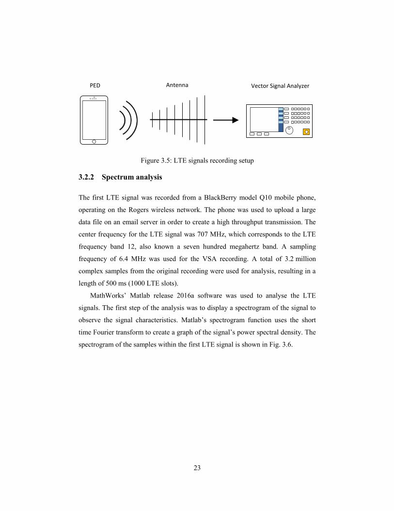
23
Figure 3.5: LTE signals recording setup
3.2.2 Spectrum analysis
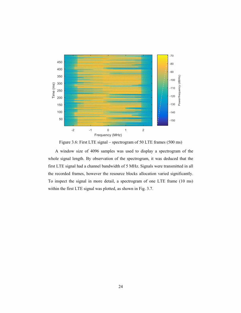
The first LTE signal was recorded from a BlackBerry model Q10 mobile phone,
operating on the Rogers wireless network. The phone was used to upload a large
data file on an email server in order to create a high throughput transmission. The
center frequency for the LTE signal was 707 MHz, which corresponds to the LTE
frequency band 12, also known a seven hundred megahertz band. A sampling
frequency of 6.4 MHz was used for the VSA recording. A total of 3.2 million
complex samples from the original recording were used for analysis, resulting in a
length of 500 ms (1000 LTE slots).
MathWorks’ Matlab release 2016a software was used to analyse the LTE
signals. The first step of the analysis was to display a spectrogram of the signal to
observe the signal characteristics. Matlab’s spectrogram function uses the short
time Fourier transform to create a graph of the signal’s power spectral density. The
spectrogram of the samples within the first LTE signal is shown in Fig. 3.6.
PED Antenna Vector Signal Analyzer
24
Figure 3.6: First LTE signal – spectrogram of 50 LTE frames (500 ms)
A window size of 4096 samples was used to display a spectrogram of the
whole signal length. By observation of the spectrogram, it was deduced that the
first LTE signal had a channel bandwidth of 5 MHz. Signals were transmitted in all
the recorded frames, however the resource blocks allocation varied significantly.
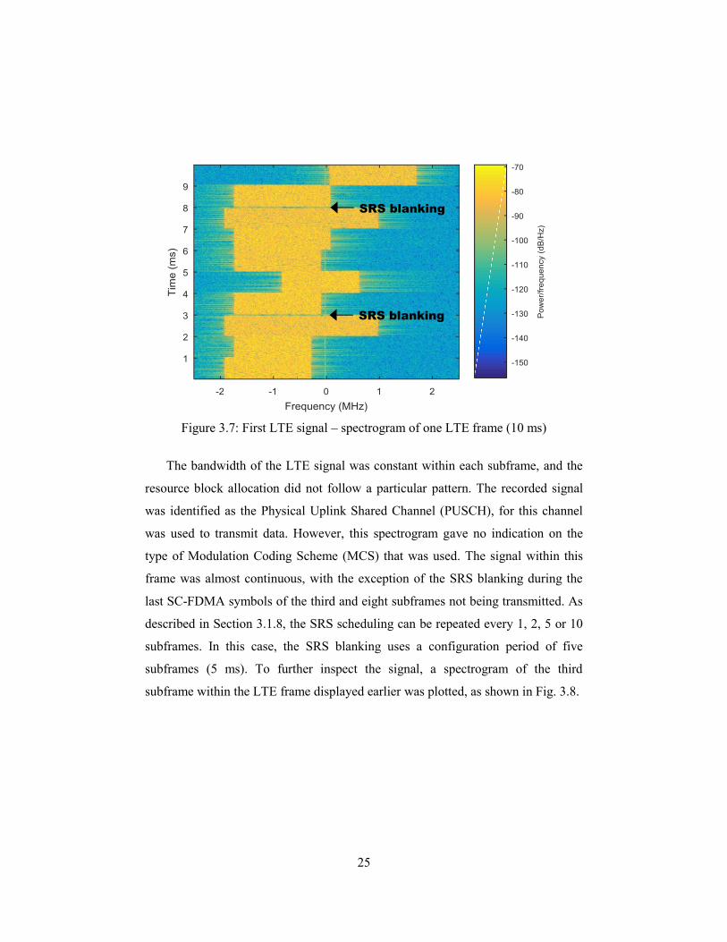
To inspect the signal in more detail, a spectrogram of one LTE frame (10 ms)
within the first LTE signal was plotted, as shown in Fig. 3.7.
25
Figure 3.7: First LTE signal – spectrogram of one LTE frame (10 ms)
The bandwidth of the LTE signal was constant within each subframe, and the
resource block allocation did not follow a particular pattern. The recorded signal
was identified as the Physical Uplink Shared Channel (PUSCH), for this channel
was used to transmit data. However, this spectrogram gave no indication on the
type of Modulation Coding Scheme (MCS) that was used. The signal within this
frame was almost continuous, with the exception of the SRS blanking during the
last SC-FDMA symbols of the third and eight subframes not being transmitted. As
described in Section 3.1.8, the SRS scheduling can be repeated every 1, 2, 5 or 10
subframes. In this case, the SRS blanking uses a configuration period of five
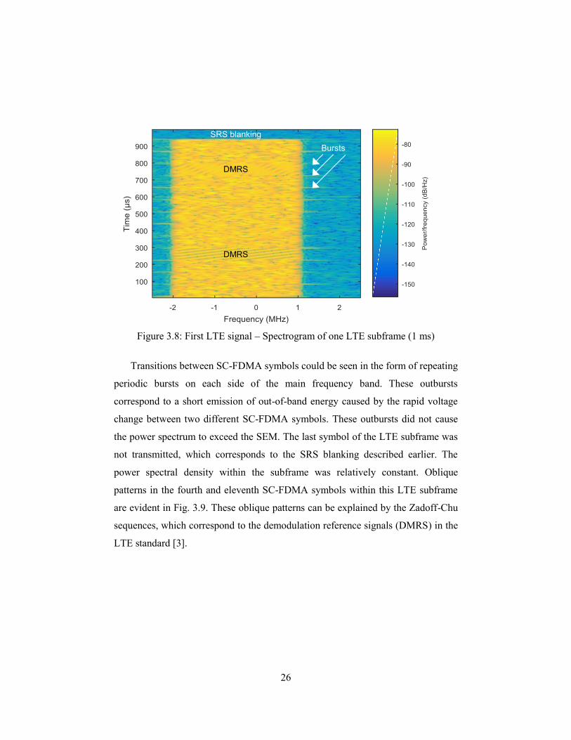
subframes (5 ms). To further inspect the signal, a spectrogram of the third
subframe within the LTE frame displayed earlier was plotted, as shown in Fig. 3.8.
SRS blanking
SRS blanking
26
Figure 3.8: First LTE signal – Spectrogram of one LTE subframe (1 ms)
Transitions between SC-FDMA symbols could be seen in the form of repeating
periodic bursts on each side of the main frequency band. These outbursts
correspond to a short emission of out-of-band energy caused by the rapid voltage
change between two different SC-FDMA symbols. These outbursts did not cause
the power spectrum to exceed the SEM. The last symbol of the LTE subframe was
not transmitted, which corresponds to the SRS blanking described earlier. The
power spectral density within the subframe was relatively constant. Oblique
patterns in the fourth and eleventh SC-FDMA symbols within this LTE subframe
are evident in Fig. 3.9. These oblique patterns can be explained by the Zadoff-Chu
sequences, which correspond to the demodulation reference signals (DMRS) in the
LTE standard [3].
SRS blanking
Bursts
DMRS
DMRS
27
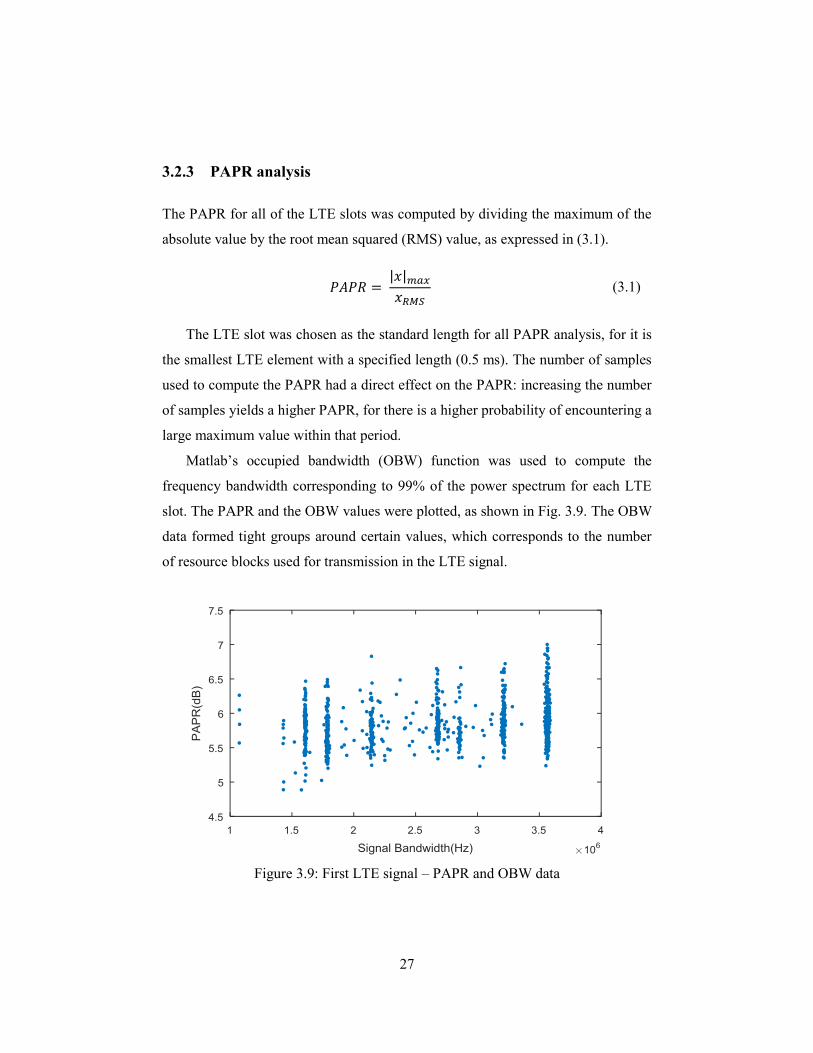
3.2.3 PAPR analysis
The PAPR for all of the LTE slots was computed by dividing the maximum of the
absolute value by the root mean squared (RMS) value, as expressed in (3.1).
| |
(3.1)
The LTE slot was chosen as the standard length for all PAPR analysis, for it is
the smallest LTE element with a specified length (0.5 ms). The number of samples
used to compute the PAPR had a direct effect on the PAPR: increasing the number
of samples yields a higher PAPR, for there is a higher probability of encountering a
large maximum value within that period.
Matlab’s occupied bandwidth (OBW) function was used to compute the
frequency bandwidth corresponding to 99% of the power spectrum for each LTE
slot. The PAPR and the OBW values were plotted, as shown in Fig. 3.9. The OBW
data formed tight groups around certain values, which corresponds to the number
of resource blocks used for transmission in the LTE signal.
Figure 3.9: First LTE signal – PAPR and OBW data
28
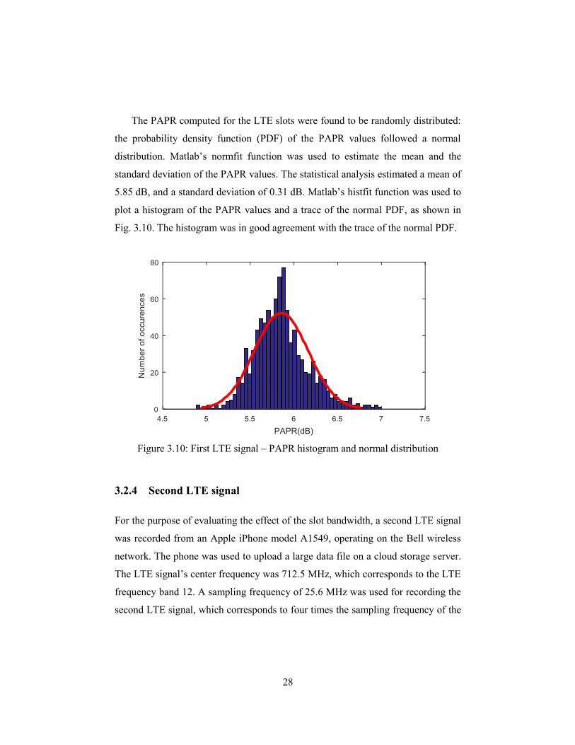
The PAPR computed for the LTE slots were found to be randomly distributed:
the probability density function (PDF) of the PAPR values followed a normal
distribution. Matlab’s normfit function was used to estimate the mean and the
standard deviation of the PAPR values. The statistical analysis estimated a mean of
5.85 dB, and a standard deviation of 0.31 dB. Matlab’s histfit function was used to
plot a histogram of the PAPR values and a trace of the normal PDF, as shown in
Fig. 3.10. The histogram was in good agreement with the trace of the normal PDF.
Figure 3.10: First LTE signal – PAPR histogram and normal distribution
3.2.4 Second LTE signal
For the purpose of evaluating the effect of the slot bandwidth, a second LTE signal
was recorded from an Apple iPhone model A1549, operating on the Bell wireless
network. The phone was used to upload a large data file on a cloud storage server.
The LTE signal’s center frequency was 712.5 MHz, which corresponds to the LTE
frequency band 12. A sampling frequency of 25.6 MHz was used for recording the
second LTE signal, which corresponds to four times the sampling frequency of the
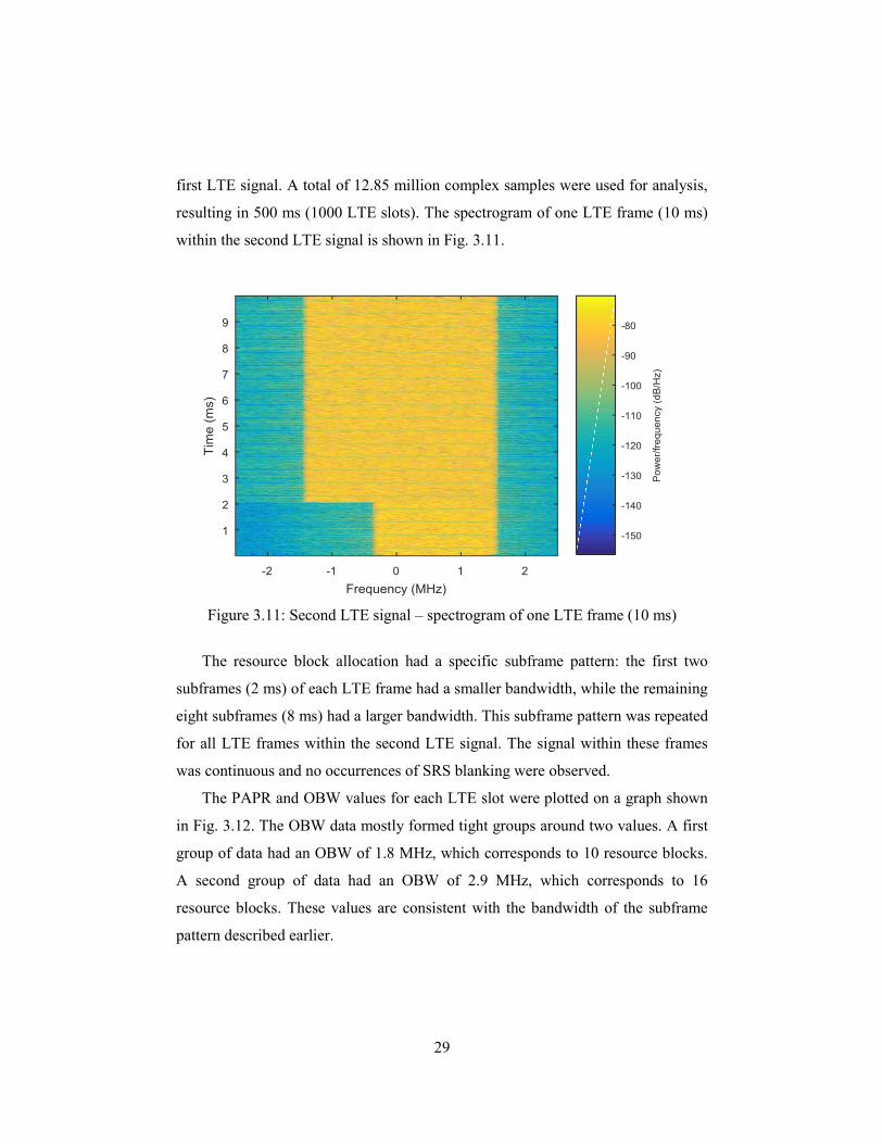
29
first LTE signal. A total of 12.85 million complex samples were used for analysis,
resulting in 500 ms (1000 LTE slots). The spectrogram of one LTE frame (10 ms)
within the second LTE signal is shown in Fig. 3.11.
Figure 3.11: Second LTE signal – spectrogram of one LTE frame (10 ms)
The resource block allocation had a specific subframe pattern: the first two
subframes (2 ms) of each LTE frame had a smaller bandwidth, while the remaining
eight subframes (8 ms) had a larger bandwidth. This subframe pattern was repeated
for all LTE frames within the second LTE signal. The signal within these frames
was continuous and no occurrences of SRS blanking were observed.
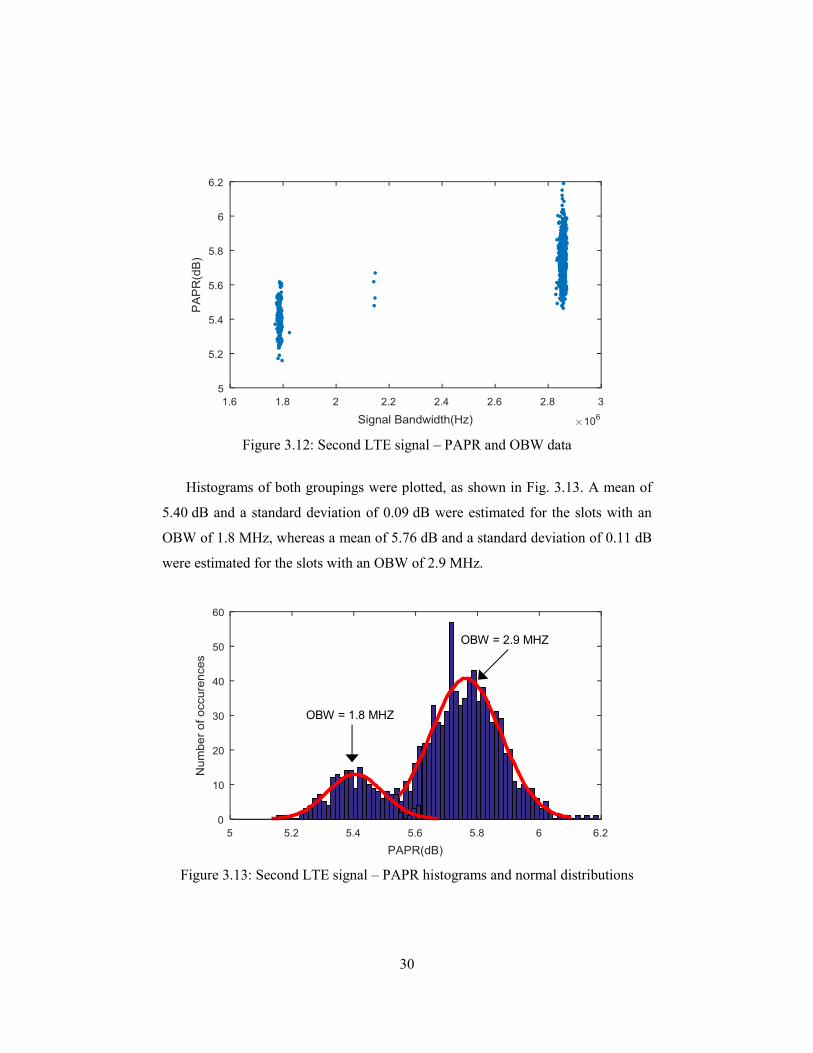
The PAPR and OBW values for each LTE slot were plotted on a graph shown
in Fig. 3.12. The OBW data mostly formed tight groups around two values. A first
group of data had an OBW of 1.8 MHz, which corresponds to 10 resource blocks.
A second group of data had an OBW of 2.9 MHz, which corresponds to 16
resource blocks. These values are consistent with the bandwidth of the subframe
pattern described earlier.
30
Figure 3.12: Second LTE signal – PAPR and OBW data
Histograms of both groupings were plotted, as shown in Fig. 3.13. A mean of
5.40 dB and a standard deviation of 0.09 dB were estimated for the slots with an
OBW of 1.8 MHz, whereas a mean of 5.76 dB and a standard deviation of 0.11 dB
were estimated for the slots with an OBW of 2.9 MHz.
Figure 3.13: Second LTE signal – PAPR histograms and normal distributions
OBW = 2.9 MHZ
OBW = 1.8 MHZ
31
Both histograms were in good agreement to the traces of the normal PDFs. It
was observed that the OBW of the LTE slots had a significant effect on the PAPR:
an increase in the OBW led to higher PAPR. This can be explained by the fact that
when the signal’s frequency is increased, there is a higher probability of
encountering a large maximum value within that period.
3.2.5 Third LTE signal
For the purpose of evaluating the effect of the MCS index on the PAPR, a third
LTE signal was recorded in similar conditions that of the second LTE signal: the
same mobile phone was used to upload a large data file on a cloud storage server.
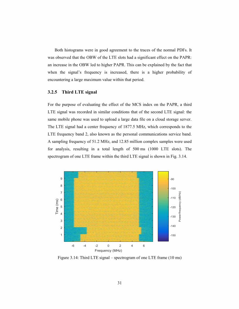
The LTE signal had a center frequency of 1877.5 MHz, which corresponds to the
LTE frequency band 2, also known as the personal communications service band.
A sampling frequency of 51.2 MHz, and 12.85 million complex samples were used
for analysis, resulting in a total length of 500 ms (1000 LTE slots). The
spectrogram of one LTE frame within the third LTE signal is shown in Fig. 3.14.
Figure 3.14: Third LTE signal – spectrogram of one LTE frame (10 ms)
32
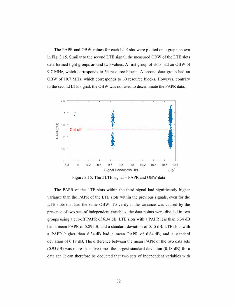
The PAPR and OBW values for each LTE slot were plotted on a graph shown
in Fig. 3.15. Similar to the second LTE signal, the measured OBW of the LTE slots
data formed tight groups around two values. A first group of slots had an OBW of
9.7 MHz, which corresponds to 54 resource blocks. A second data group had an
OBW of 10.7 MHz, which corresponds to 60 resource blocks. However, contrary
to the second LTE signal, the OBW was not used to discriminate the PAPR data.
Figure 3.15: Third LTE signal – PAPR and OBW data
The PAPR of the LTE slots within the third signal had significantly higher
variance than the PAPR of the LTE slots within the previous signals, even for the
LTE slots that had the same OBW. To verify if the variance was caused by the
presence of two sets of independent variables, the data points were divided in two
groups using a cut-off PAPR of 6.34 dB. LTE slots with a PAPR less than 6.34 dB
had a mean PAPR of 5.89 dB, and a standard deviation of 0.15 dB. LTE slots with
a PAPR higher than 6.34 dB had a mean PAPR of 6.84 dB, and a standard
deviation of 0.18 dB. The difference between the mean PAPR of the two data sets
(0.95 dB) was more than five times the largest standard deviation (0.18 dB) for a
data set. It can therefore be deducted that two sets of independent variables with
Cut-off
33
different signal parameters are present. It is hypothesized that the modulation
coding scheme (MCS) varied within the LTE signal, and that it had an effect on the
measured PAPR. For example, some LTE slots could have a lower MCS index
associated with a QPSK modulation, while other LTE slots could have a higher
MCS index associated with a 16QAM modulation.
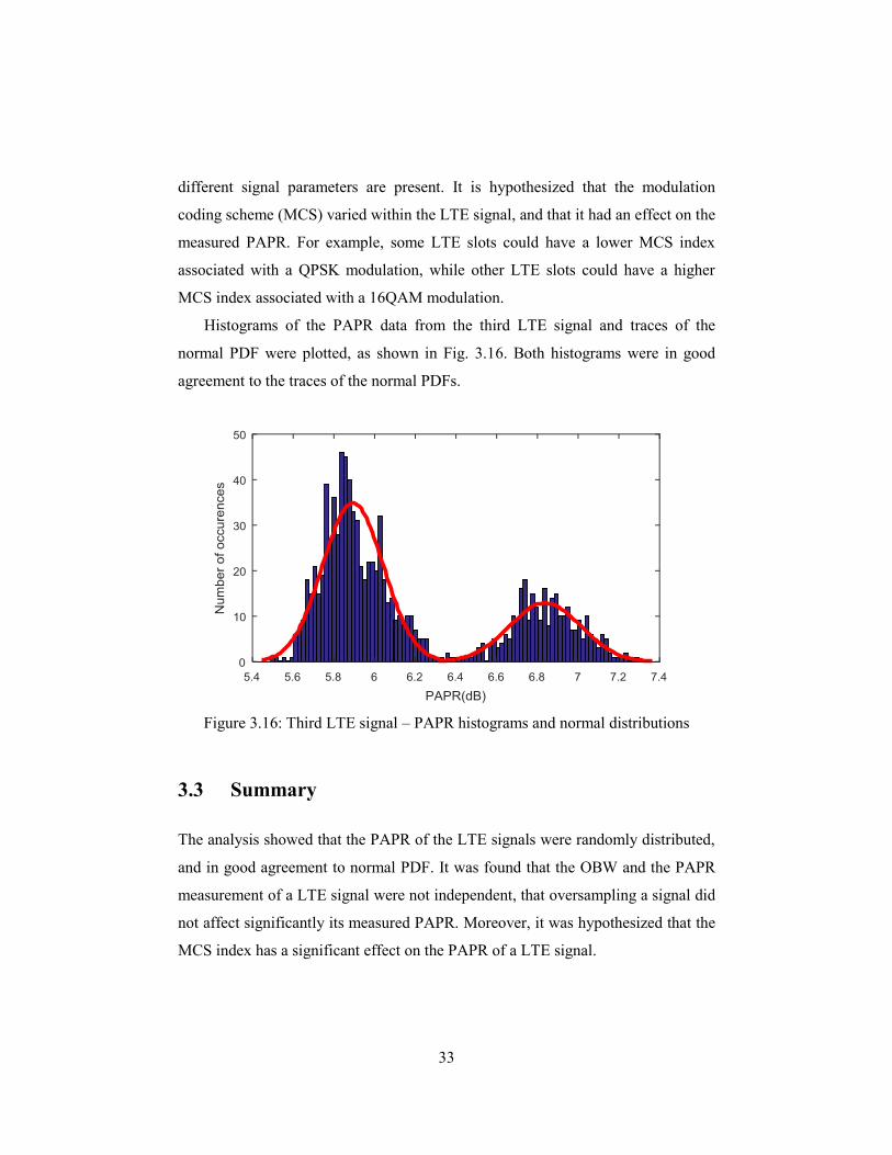
Histograms of the PAPR data from the third LTE signal and traces of the
normal PDF were plotted, as shown in Fig. 3.16. Both histograms were in good
agreement to the traces of the normal PDFs.
Figure 3.16: Third LTE signal – PAPR histograms and normal distributions
3.3 Summary
The analysis showed that the PAPR of the LTE signals were randomly distributed,
and in good agreement to normal PDF. It was found that the OBW and the PAPR
measurement of a LTE signal were not independent, that oversampling a signal did
not affect significantly its measured PAPR. Moreover, it was hypothesized that the
MCS index has a significant effect on the PAPR of a LTE signal.
34
4 Test waveform design
Chapter 3 described the complexity of the LTE standard. This chapter will cover
the design of test waveforms that are suitable for radiated susceptibility testing. To
ensure that each test waveform is representative of the LTE standard, their power
spectrum will be compared to the spectrum emission mask (SEM). The PAPR of
the test waveforms will also be analyzed, in order to select the parameters that
could yield the most significant results during radiated susceptibility testing.
4.1 Methodology and considerations
DO294C provided some guidance for the design of test waveforms of complex
communication standards such as LTE [4]. It claimed that the highest interference
threat is linked to signals with pulse modulation: the fast change in amplitude was
alleged to have the greatest effect on the susceptibility of the victims. Amplitude
changes caused by digital modulation schemes such as QAM were said to increase
the susceptibility of victim systems, but with less effect than pulse modulation.
DO294C argued that frequency and phase changes caused by digital modulation do
not have a significant effect on the susceptibility, suggesting that phase shift keying
can be modeled by a continuous wave. Moreover, DO294C claimed that the
waveform duty cycle does not have a significant effect on the susceptibility, and
that the effect of the peak power is more significant than that of the signal energy.
Previous studies on radiated susceptibility also provided insights for the design
of test waveforms. The study performed at NTT DoCoMo found that variations in
the PAPR did not have a significant effect on the susceptibility [10]. However, this
observation has not been replicated. It is suspected that a high PAPR can induce a
higher susceptibility on victim systems, but that to measure its effect, the test
waveforms parameters must be controlled using an appropriate methodology.
35
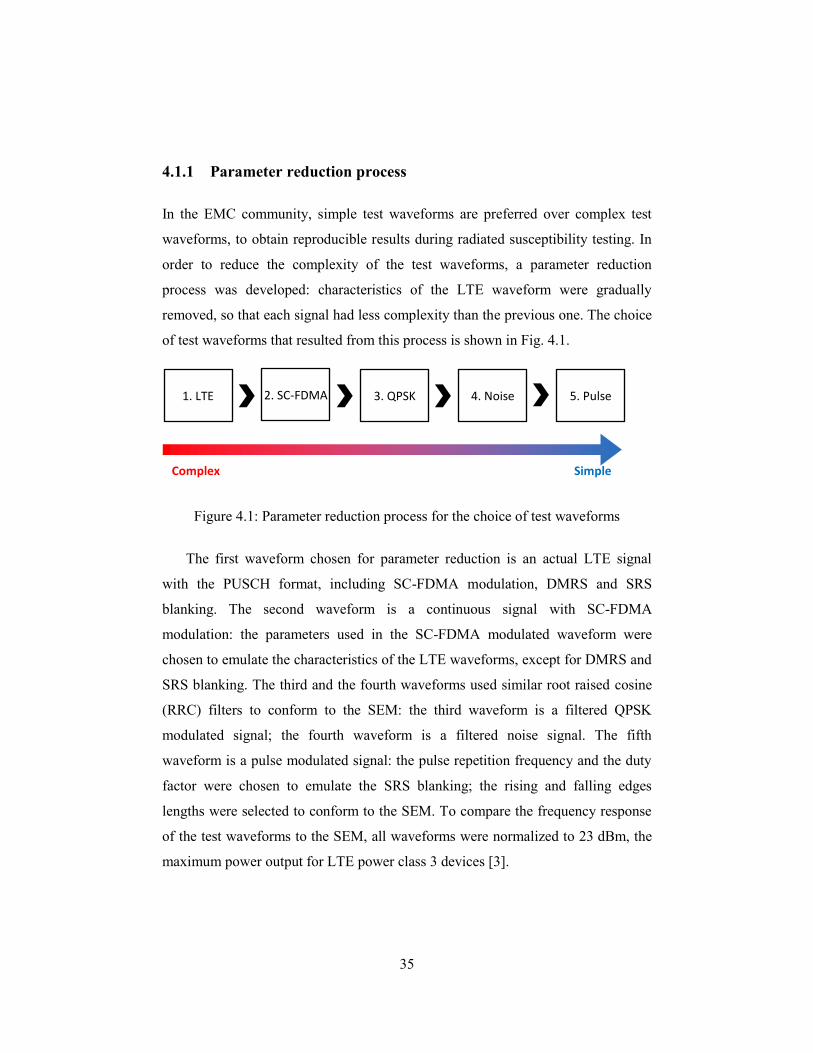
4.1.1 Parameter reduction process
In the EMC community, simple test waveforms are preferred over complex test
waveforms, to obtain reproducible results during radiated susceptibility testing. In
order to reduce the complexity of the test waveforms, a parameter reduction
process was developed: characteristics of the LTE waveform were gradually
removed, so that each signal had less complexity than the previous one. The choice
of test waveforms that resulted from this process is shown in Fig. 4.1.
Figure 4.1: Parameter reduction process for the choice of test waveforms
The first waveform chosen for parameter reduction is an actual LTE signal
with the PUSCH format, including SC-FDMA modulation, DMRS and SRS
blanking. The second waveform is a continuous signal with SC-FDMA
modulation: the parameters used in the SC-FDMA modulated waveform were
chosen to emulate the characteristics of the LTE waveforms, except for DMRS and
SRS blanking. The third and the fourth waveforms used similar root raised cosine
(RRC) filters to conform to the SEM: the third waveform is a filtered QPSK
modulated signal; the fourth waveform is a filtered noise signal. The fifth
waveform is a pulse modulated signal: the pulse repetition frequency and the duty
factor were chosen to emulate the SRS blanking; the rising and falling edges
lengths were selected to conform to the SEM. To compare the frequency response
of the test waveforms to the SEM, all waveforms were normalized to 23 dBm, the
maximum power output for LTE power class 3 devices [3].
1. LTE 2. SC-FDMA 3. QPSK 4. Noise 5. Pulse
Complex Simple
36
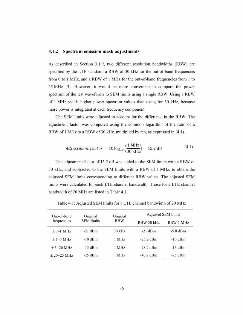
4.1.2 Spectrum emission mask adjustments
As described in Section 3.1.9, two different resolution bandwidths (RBW) are
specified by the LTE standard: a RBW of 30 kHz for the out-of-band frequencies
from 0 to 1 MHz, and a RBW of 1 MHz for the out-of-band frequencies from 1 to
25 MHz [3]. However, it would be more convenient to compare the power
spectrum of the test waveforms to SEM limits using a single RBW. Using a RBW
of 1 MHz yields higher power spectrum values than using for 30 kHz, because
more power is integrated at each frequency component.
The SEM limits were adjusted to account for the difference in the RBW. The
adjustment factor was computed using the common logarithm of the ratio of a
RBW of 1 MHz to a RBW of 30 kHz, multiplied by ten, as expressed in (4.1).
(
) (4.1)
The adjustment factor of 15.2 dB was added to the SEM limits with a RBW of
30 kHz, and subtracted to the SEM limits with a RBW of 1 MHz, to obtain the
adjusted SEM limits corresponding to different RBW values. The adjusted SEM
limits were calculated for each LTE channel bandwidth. Those for a LTE channel
bandwidth of 20 MHz are listed in Table 4.1.
Table 4.1: Adjusted SEM limits for a LTE channel bandwidth of 20 MHz
Out-of-band
frequencies
Original
SEM limits
Original
RBW
Adjusted SEM limits
RBW 30 kHz RBW 1 MHz
MHz -21 dBm 30 kHz -21 dBm -5.8 dBm
MHz -10 dBm 1 MHz -25.2 dBm -10 dBm
20 MHz -13 dBm 1 MHz -28.2 dBm -13 dBm
2025 MHz -25 dBm 1 MHz -40.2 dBm -25 dBm
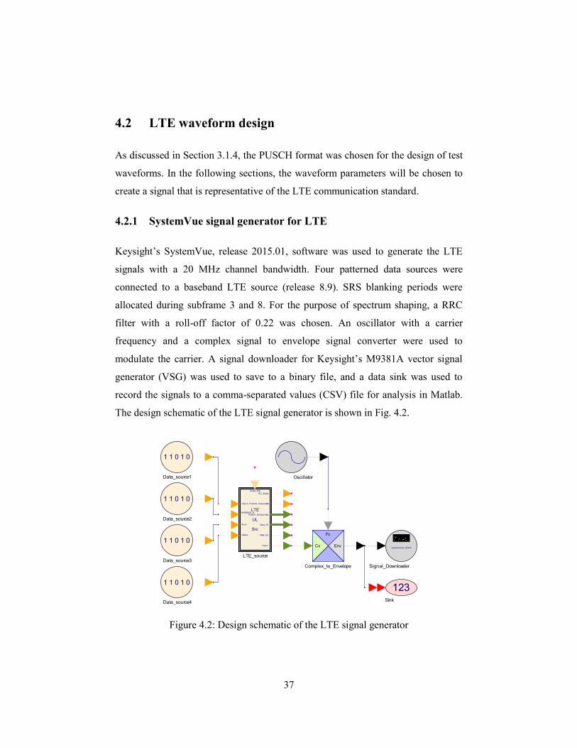
37
4.2 LTE waveform design
As discussed in Section 3.1.4, the PUSCH format was chosen for the design of test
waveforms. In the following sections, the waveform parameters will be chosen to
create a signal that is representative of the LTE communication standard.
4.2.1 SystemVue signal generator for LTE
Keysight’s SystemVue, release 2015.01, software was used to generate the LTE
signals with a 20 MHz channel bandwidth. Four patterned data sources were
connected to a baseband LTE source (release 8.9). SRS blanking periods were
allocated during subframe 3 and 8. For the purpose of spectrum shaping, a RRC
filter with a roll-off factor of 0.22 was chosen. An oscillator with a carrier
frequency and a complex signal to envelope signal converter were used to
modulate the carrier. A signal downloader for Keysight’s M9381A vector signal
generator (VSG) was used to save to a binary file, and a data sink was used to
record the signals to a comma-separated values (CSV) file for analysis in Matlab.
The design schematic of the LTE signal generator is shown in Fig. 4.2.
Figure 4.2: Design schematic of the LTE signal generator
Fc
EnvCx
Complex_to_Envelope
1 1 0 1 0
Data_source3
1 1 0 1 0
Data_source2
1 1 0 1 0
Data_source1
1 1 0 1 0
Data_source4
Oscillator
123Sink
SignalDownloader_M9381A
Signal_Downloader
HARQ_Bits
DataIn
RI_In
HARQACK_In
CQI_In
Frame
FRM_FD
Data_FD
PUSCH_ModSymbols
SC_Status
PUSCH_ChannelBits
LTE
UL
Src
LTE_source
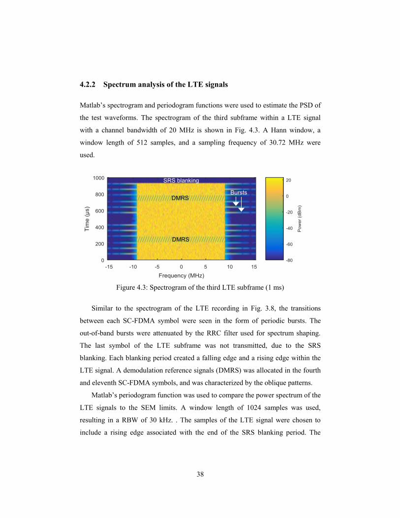
38
4.2.2 Spectrum analysis of the LTE signals
Matlab’s spectrogram and periodogram functions were used to estimate the PSD of
the test waveforms. The spectrogram of the third subframe within a LTE signal
with a channel bandwidth of 20 MHz is shown in Fig. 4.3. A Hann window, a
window length of 512 samples, and a sampling frequency of 30.72 MHz were
used.
Figure 4.3: Spectrogram of the third LTE subframe (1 ms)
Similar to the spectrogram of the LTE recording in Fig. 3.8, the transitions
between each SC-FDMA symbol were seen in the form of periodic bursts. The
out-of-band bursts were attenuated by the RRC filter used for spectrum shaping.
The last symbol of the LTE subframe was not transmitted, due to the SRS
blanking. Each blanking period created a falling edge and a rising edge within the
LTE signal. A demodulation reference signals (DMRS) was allocated in the fourth
and eleventh SC-FDMA symbols, and was characterized by the oblique patterns.
Matlab’s periodogram function was used to compare the power spectrum of the
LTE signals to the SEM limits. A window length of 1024 samples was used,
resulting in a RBW of 30 kHz. . The samples of the LTE signal were chosen to
include a rising edge associated with the end of the SRS blanking period. The
SRS blanking
DMRS
DMRS
Bursts
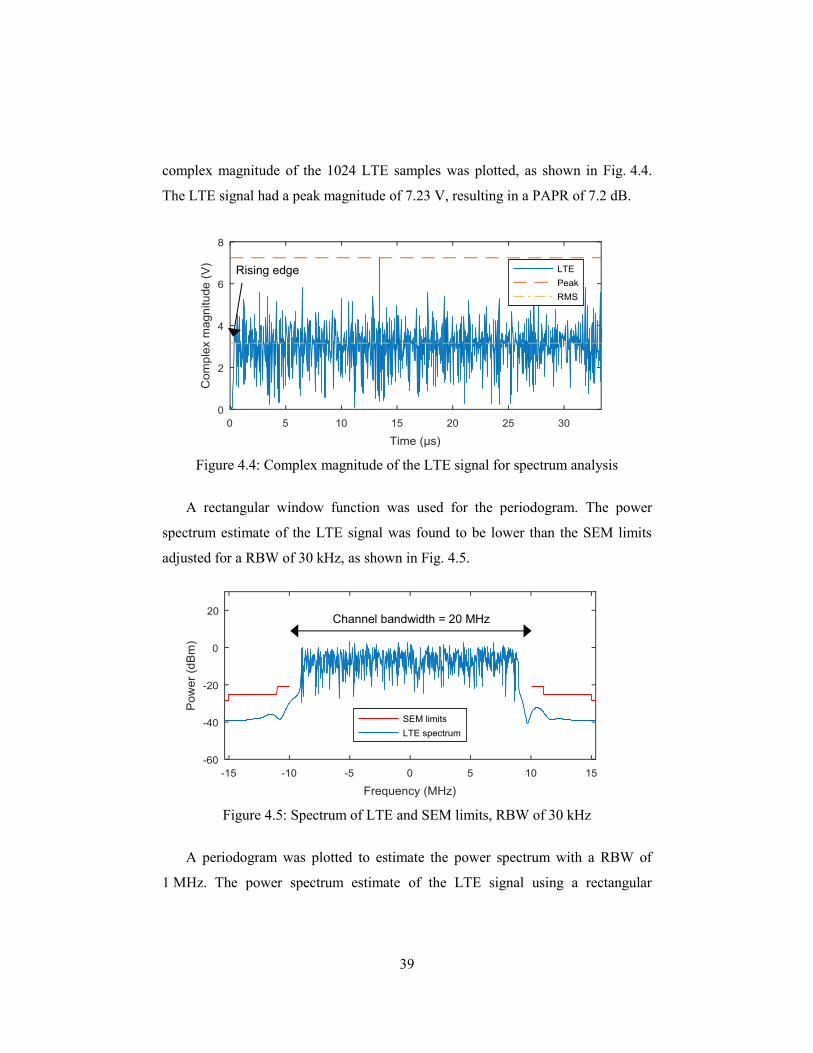
39
complex magnitude of the 1024 LTE samples was plotted, as shown in Fig. 4.4.
The LTE signal had a peak magnitude of 7.23 V, resulting in a PAPR of 7.2 dB.
Figure 4.4: Complex magnitude of the LTE signal for spectrum analysis
A rectangular window function was used for the periodogram. The power
spectrum estimate of the LTE signal was found to be lower than the SEM limits
adjusted for a RBW of 30 kHz, as shown in Fig. 4.5.
Figure 4.5: Spectrum of LTE and SEM limits, RBW of 30 kHz
A periodogram was plotted to estimate the power spectrum with a RBW of
1 MHz. The power spectrum estimate of the LTE signal using a rectangular
Channel bandwidth = 20 MHz
Rising edge
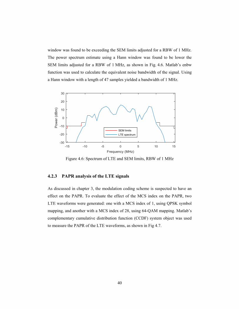
40
window was found to be exceeding the SEM limits adjusted for a RBW of 1 MHz.
The power spectrum estimate using a Hann window was found to be lower the
SEM limits adjusted for a RBW of 1 MHz, as shown in Fig. 4.6. Matlab’s enbw
function was used to calculate the equivalent noise bandwidth of the signal. Using
a Hann window with a length of 47 samples yielded a bandwidth of 1 MHz.
Figure 4.6: Spectrum of LTE and SEM limits, RBW of 1 MHz
4.2.3 PAPR analysis of the LTE signals
As discussed in chapter 3, the modulation coding scheme is suspected to have an
effect on the PAPR. To evaluate the effect of the MCS index on the PAPR, two
LTE waveforms were generated: one with a MCS index of 1, using QPSK symbol
mapping, and another with a MCS index of 28, using 64-QAM mapping. Matlab’s
complementary cumulative distribution function (CCDF) system object was used
to measure the PAPR of the LTE waveforms, as shown in Fig 4.7.
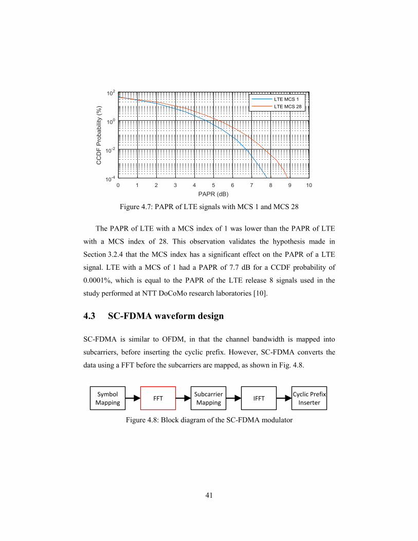
41
Figure 4.7: PAPR of LTE signals with MCS 1 and MCS 28
The PAPR of LTE with a MCS index of 1 was lower than the PAPR of LTE
with a MCS index of 28. This observation validates the hypothesis made in
Section 3.2.4 that the MCS index has a significant effect on the PAPR of a LTE
signal. LTE with a MCS of 1 had a PAPR of 7.7 dB for a CCDF probability of
0.0001%, which is equal to the PAPR of the LTE release 8 signals used in the
study performed at NTT DoCoMo research laboratories [10].
4.3 SC-FDMA waveform design
SC-FDMA is similar to OFDM, in that the channel bandwidth is mapped into
subcarriers, before inserting the cyclic prefix. However, SC-FDMA converts the
data using a FFT before the subcarriers are mapped, as shown in Fig. 4.8.
Figure 4.8: Block diagram of the SC-FDMA modulator
Symbol Mapping
FFT Subcarrier Mapping
IFFT Cyclic Prefix
Inserter
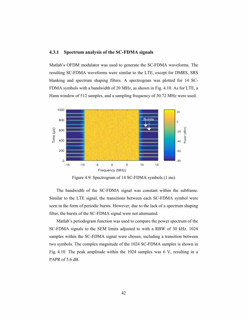
42
4.3.1 Spectrum analysis of the SC-FDMA signals
Matlab’s OFDM modulator was used to generate the SC-FDMA waveforms. The
resulting SC-FDMA waveforms were similar to the LTE, except for DMRS, SRS
blanking and spectrum shaping filters. A spectrogram was plotted for 14 SC-
FDMA symbols with a bandwidth of 20 MHz, as shown in Fig. 4.10. As for LTE, a
Hann window of 512 samples, and a sampling frequency of 30.72 MHz were used.
Figure 4.9: Spectrogram of 14 SC-FDMA symbols (1 ms)
The bandwidth of the SC-FDMA signal was constant within the subframe.
Similar to the LTE signal, the transitions between each SC-FDMA symbol were
seen in the form of periodic bursts. However, due to the lack of a spectrum shaping
filter, the bursts of the SC-FDMA signal were not attenuated.
Matlab’s periodogram function was used to compare the power spectrum of the
SC-FDMA signals to the SEM limits adjusted to with a RBW of 30 kHz. 1024
samples within the SC-FDMA signal were chosen, including a transition between
two symbols. The complex magnitude of the 1024 SC-FDMA samples is shown in
Fig. 4.10. The peak amplitude within the 1024 samples was 6 V, resulting in a
PAPR of 5.6 dB.
Bursts
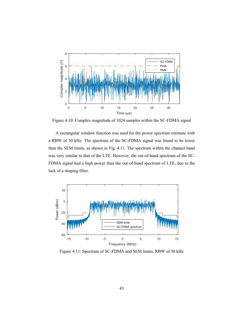
43
Figure 4.10: Complex magnitude of 1024 samples within the SC-FDMA signal
A rectangular window function was used for the power spectrum estimate with
a RBW of 30 kHz. The spectrum of the SC-FDMA signal was found to be lower
than the SEM limits, as shown in Fig. 4.11. The spectrum within the channel band
was very similar to that of the LTE. However, the out-of-band spectrum of the SC-
FDMA signal had a high power than the out-of-band spectrum of LTE, due to the
lack of a shaping filter.
Figure 4.11: Spectrum of SC-FDMA and SEM limits, RBW of 30 kHz
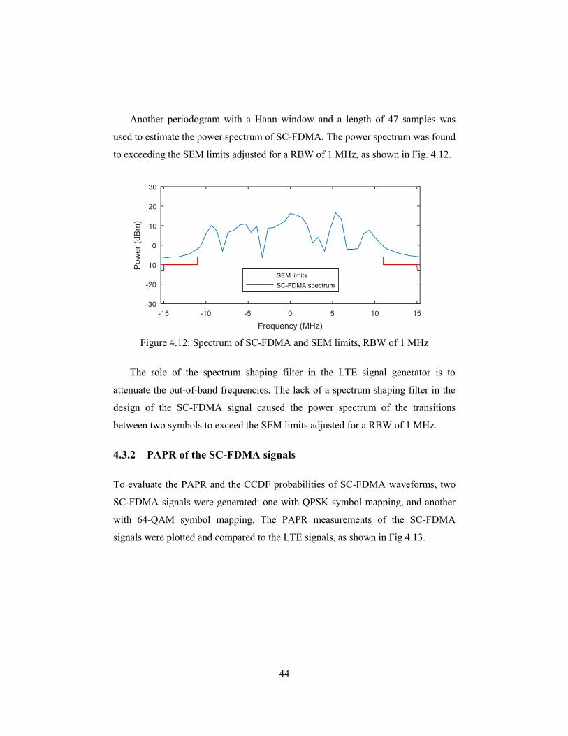
44
Another periodogram with a Hann window and a length of 47 samples was
used to estimate the power spectrum of SC-FDMA. The power spectrum was found
to exceeding the SEM limits adjusted for a RBW of 1 MHz, as shown in Fig. 4.12.
Figure 4.12: Spectrum of SC-FDMA and SEM limits, RBW of 1 MHz
The role of the spectrum shaping filter in the LTE signal generator is to
attenuate the out-of-band frequencies. The lack of a spectrum shaping filter in the
design of the SC-FDMA signal caused the power spectrum of the transitions
between two symbols to exceed the SEM limits adjusted for a RBW of 1 MHz.
4.3.2 PAPR of the SC-FDMA signals
To evaluate the PAPR and the CCDF probabilities of SC-FDMA waveforms, two
SC-FDMA signals were generated: one with QPSK symbol mapping, and another
with 64-QAM symbol mapping. The PAPR measurements of the SC-FDMA
signals were plotted and compared to the LTE signals, as shown in Fig 4.13.
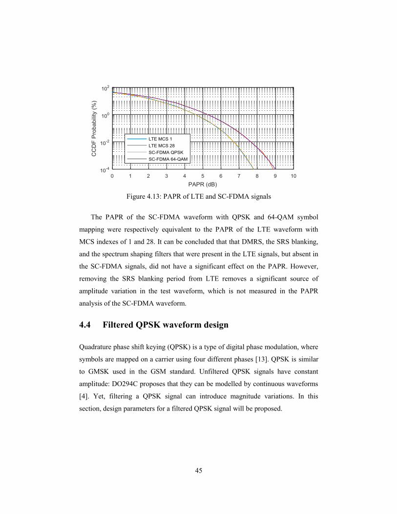
45
Figure 4.13: PAPR of LTE and SC-FDMA signals
The PAPR of the SC-FDMA waveform with QPSK and 64-QAM symbol
mapping were respectively equivalent to the PAPR of the LTE waveform with
MCS indexes of 1 and 28. It can be concluded that that DMRS, the SRS blanking,
and the spectrum shaping filters that were present in the LTE signals, but absent in
the SC-FDMA signals, did not have a significant effect on the PAPR. However,
removing the SRS blanking period from LTE removes a significant source of
amplitude variation in the test waveform, which is not measured in the PAPR
analysis of the SC-FDMA waveform.
4.4 Filtered QPSK waveform design
Quadrature phase shift keying (QPSK) is a type of digital phase modulation, where
symbols are mapped on a carrier using four different phases [13]. QPSK is similar
to GMSK used in the GSM standard. Unfiltered QPSK signals have constant
amplitude: DO294C proposes that they can be modelled by continuous waveforms
[4]. Yet, filtering a QPSK signal can introduce magnitude variations. In this
section, design parameters for a filtered QPSK signal will be proposed.
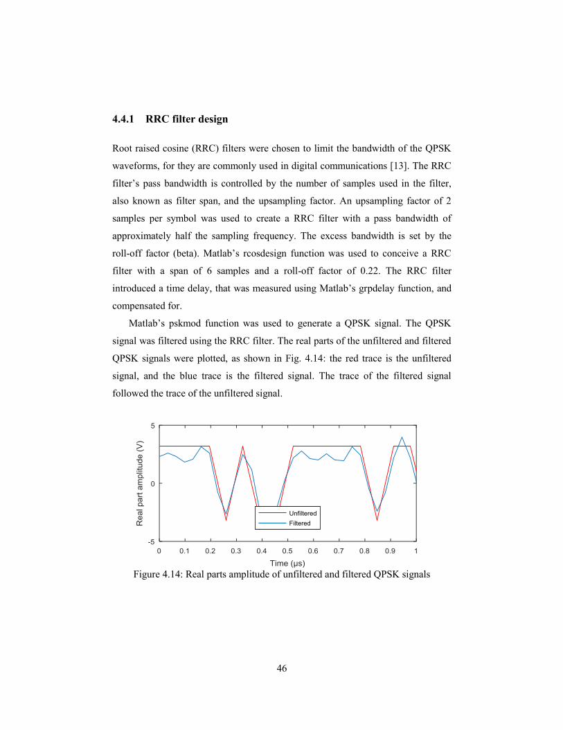
46
4.4.1 RRC filter design
Root raised cosine (RRC) filters were chosen to limit the bandwidth of the QPSK
waveforms, for they are commonly used in digital communications [13]. The RRC
filter’s pass bandwidth is controlled by the number of samples used in the filter,
also known as filter span, and the upsampling factor. An upsampling factor of 2
samples per symbol was used to create a RRC filter with a pass bandwidth of
approximately half the sampling frequency. The excess bandwidth is set by the
roll-off factor (beta). Matlab’s rcosdesign function was used to conceive a RRC
filter with a span of 6 samples and a roll-off factor of 0.22. The RRC filter
introduced a time delay, that was measured using Matlab’s grpdelay function, and
compensated for.
Matlab’s pskmod function was used to generate a QPSK signal. The QPSK
signal was filtered using the RRC filter. The real parts of the unfiltered and filtered
QPSK signals were plotted, as shown in Fig. 4.14: the red trace is the unfiltered
signal, and the blue trace is the filtered signal. The trace of the filtered signal
followed the trace of the unfiltered signal.
Figure 4.14: Real parts amplitude of unfiltered and filtered QPSK signals
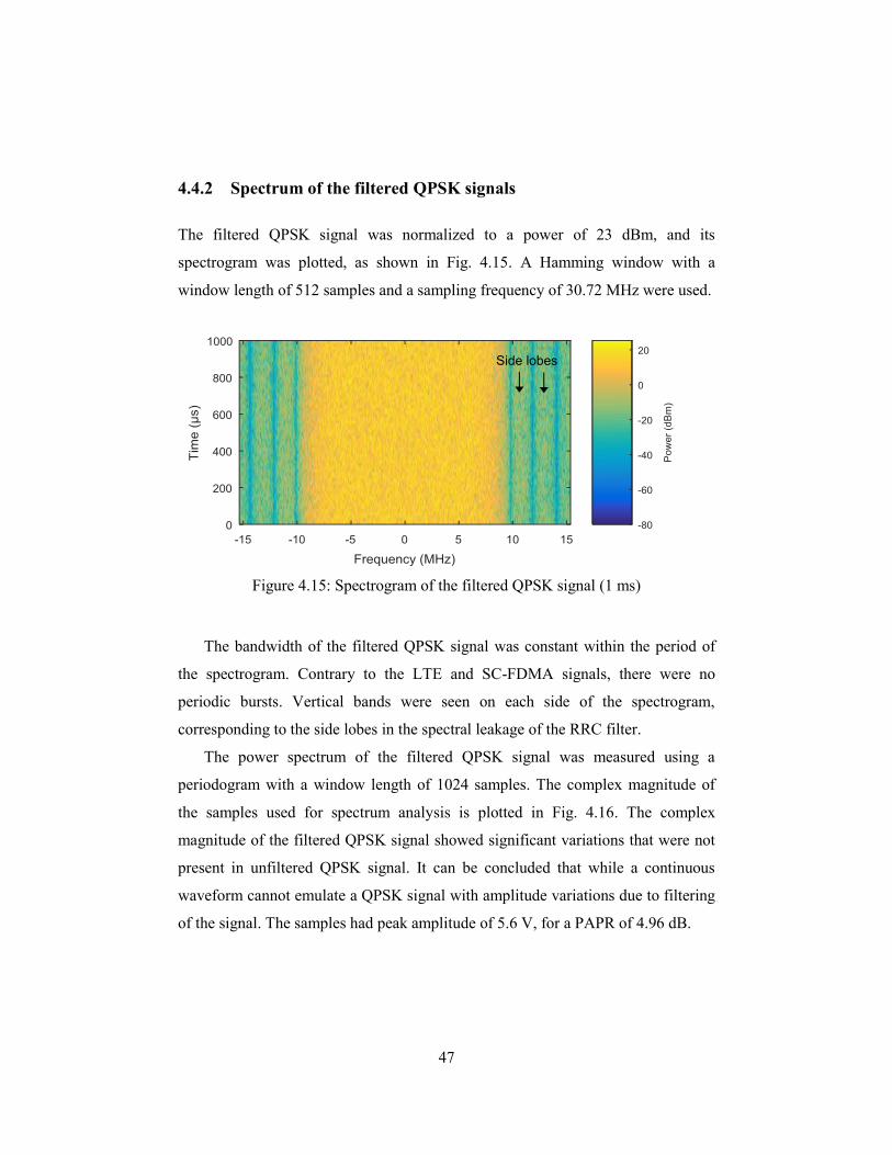
47
4.4.2 Spectrum of the filtered QPSK signals
The filtered QPSK signal was normalized to a power of 23 dBm, and its
spectrogram was plotted, as shown in Fig. 4.15. A Hamming window with a
window length of 512 samples and a sampling frequency of 30.72 MHz were used.
Figure 4.15: Spectrogram of the filtered QPSK signal (1 ms)
The bandwidth of the filtered QPSK signal was constant within the period of
the spectrogram. Contrary to the LTE and SC-FDMA signals, there were no
periodic bursts. Vertical bands were seen on each side of the spectrogram,
corresponding to the side lobes in the spectral leakage of the RRC filter.
The power spectrum of the filtered QPSK signal was measured using a
periodogram with a window length of 1024 samples. The complex magnitude of
the samples used for spectrum analysis is plotted in Fig. 4.16. The complex
magnitude of the filtered QPSK signal showed significant variations that were not
present in unfiltered QPSK signal. It can be concluded that while a continuous
waveform cannot emulate a QPSK signal with amplitude variations due to filtering
of the signal. The samples had peak amplitude of 5.6 V, for a PAPR of 4.96 dB.
Side lobes
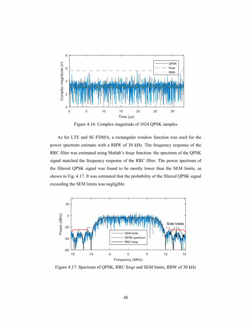
48
Figure 4.16: Complex magnitude of 1024 QPSK samples
As for LTE and SC-FDMA, a rectangular window function was used for the
power spectrum estimate with a RBW of 30 kHz. The frequency response of the
RRC filter was estimated using Matlab’s freqz function: the spectrum of the QPSK
signal matched the frequency response of the RRC filter. The power spectrum of
the filtered QPSK signal was found to be mostly lower than the SEM limits, as
shown in Fig. 4.17. It was estimated that the probability of the filtered QPSK signal
exceeding the SEM limits was negligible.
Figure 4.17: Spectrum of QPSK, RRC freqz and SEM limits, RBW of 30 kHz
Side lobes
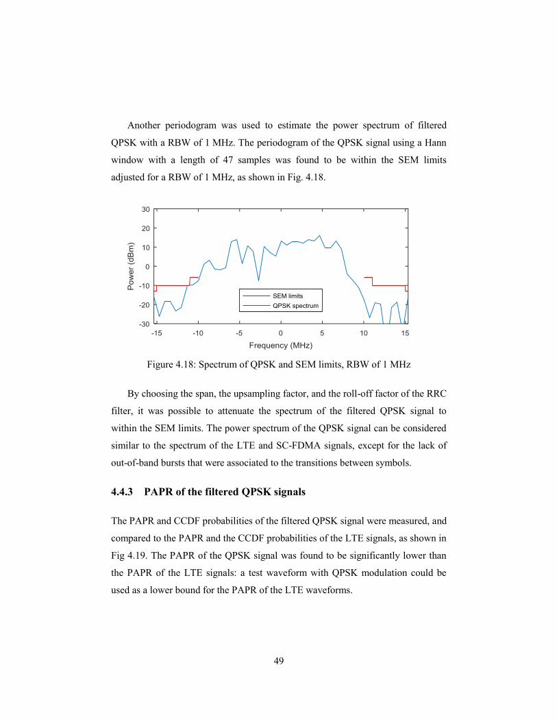
49
Another periodogram was used to estimate the power spectrum of filtered
QPSK with a RBW of 1 MHz. The periodogram of the QPSK signal using a Hann
window with a length of 47 samples was found to be within the SEM limits
adjusted for a RBW of 1 MHz, as shown in Fig. 4.18.
Figure 4.18: Spectrum of QPSK and SEM limits, RBW of 1 MHz
By choosing the span, the upsampling factor, and the roll-off factor of the RRC
filter, it was possible to attenuate the spectrum of the filtered QPSK signal to
within the SEM limits. The power spectrum of the QPSK signal can be considered
similar to the spectrum of the LTE and SC-FDMA signals, except for the lack of
out-of-band bursts that were associated to the transitions between symbols.
4.4.3 PAPR of the filtered QPSK signals
The PAPR and CCDF probabilities of the filtered QPSK signal were measured, and
compared to the PAPR and the CCDF probabilities of the LTE signals, as shown in
Fig 4.19. The PAPR of the QPSK signal was found to be significantly lower than
the PAPR of the LTE signals: a test waveform with QPSK modulation could be
used as a lower bound for the PAPR of the LTE waveforms.
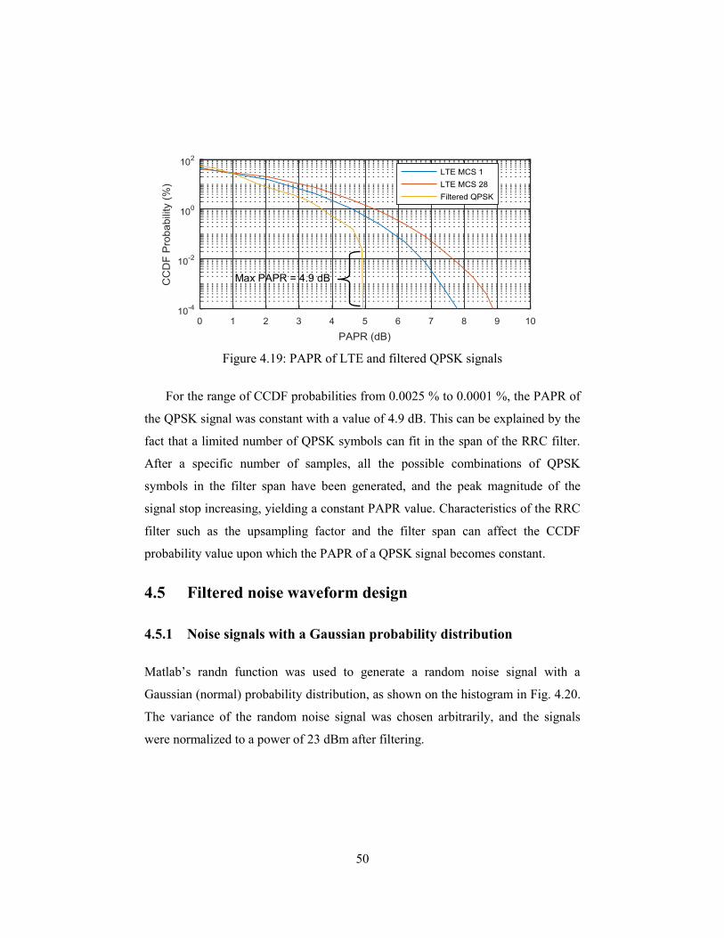
50
Figure 4.19: PAPR of LTE and filtered QPSK signals
For the range of CCDF probabilities from 0.0025 % to 0.0001 %, the PAPR of
the QPSK signal was constant with a value of 4.9 dB. This can be explained by the
fact that a limited number of QPSK symbols can fit in the span of the RRC filter.
After a specific number of samples, all the possible combinations of QPSK
symbols in the filter span have been generated, and the peak magnitude of the
signal stop increasing, yielding a constant PAPR value. Characteristics of the RRC
filter such as the upsampling factor and the filter span can affect the CCDF
probability value upon which the PAPR of a QPSK signal becomes constant.
4.5 Filtered noise waveform design
4.5.1 Noise signals with a Gaussian probability distribution
Matlab’s randn function was used to generate a random noise signal with a
Gaussian (normal) probability distribution, as shown on the histogram in Fig. 4.20.
The variance of the random noise signal was chosen arbitrarily, and the signals
were normalized to a power of 23 dBm after filtering.
Max PAPR = 4.9 dB
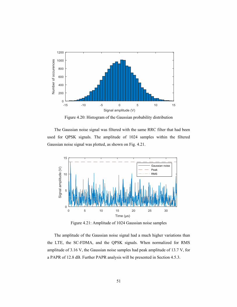
51
Figure 4.20: Histogram of the Gaussian probability distribution
The Gaussian noise signal was filtered with the same RRC filter that had been
used for QPSK signals. The amplitude of 1024 samples within the filtered
Gaussian noise signal was plotted, as shown on Fig. 4.21.
Figure 4.21: Amplitude of 1024 Gaussian noise samples
The amplitude of the Gaussian noise signal had a much higher variations than
the LTE, the SC-FDMA, and the QPSK signals. When normalized for RMS
amplitude of 3.16 V, the Gaussian noise samples had peak amplitude of 13.7 V, for
a PAPR of 12.8 dB. Further PAPR analysis will be presented in Section 4.5.3.
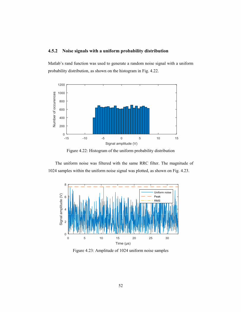
52
4.5.2 Noise signals with a uniform probability distribution
Matlab’s rand function was used to generate a random noise signal with a uniform
probability distribution, as shown on the histogram in Fig. 4.22.
Figure 4.22: Histogram of the uniform probability distribution
The uniform noise was filtered with the same RRC filter. The magnitude of
1024 samples within the uniform noise signal was plotted, as shown on Fig. 4.23.
Figure 4.23: Amplitude of 1024 uniform noise samples
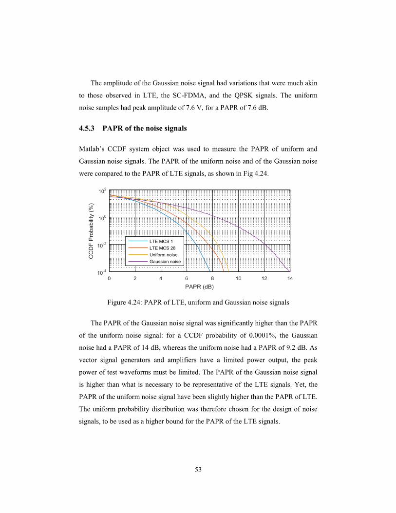
53
The amplitude of the Gaussian noise signal had variations that were much akin
to those observed in LTE, the SC-FDMA, and the QPSK signals. The uniform
noise samples had peak amplitude of 7.6 V, for a PAPR of 7.6 dB.
4.5.3 PAPR of the noise signals
Matlab’s CCDF system object was used to measure the PAPR of uniform and
Gaussian noise signals. The PAPR of the uniform noise and of the Gaussian noise
were compared to the PAPR of LTE signals, as shown in Fig 4.24.
Figure 4.24: PAPR of LTE, uniform and Gaussian noise signals
The PAPR of the Gaussian noise signal was significantly higher than the PAPR
of the uniform noise signal: for a CCDF probability of 0.0001%, the Gaussian
noise had a PAPR of 14 dB, whereas the uniform noise had a PAPR of 9.2 dB. As
vector signal generators and amplifiers have a limited power output, the peak
power of test waveforms must be limited. The PAPR of the Gaussian noise signal
is higher than what is necessary to be representative of the LTE signals. Yet, the
PAPR of the uniform noise signal have been slightly higher than the PAPR of LTE.
The uniform probability distribution was therefore chosen for the design of noise
signals, to be used as a higher bound for the PAPR of the LTE signals.
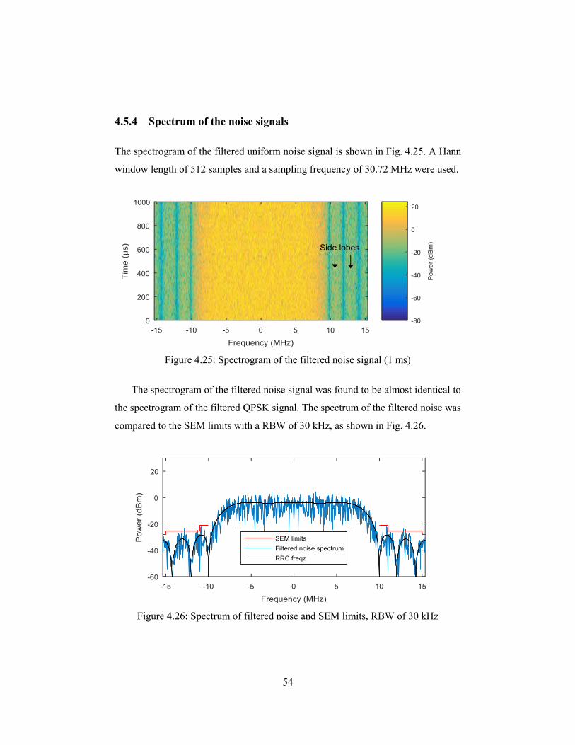
54
4.5.4 Spectrum of the noise signals
The spectrogram of the filtered uniform noise signal is shown in Fig. 4.25. A Hann
window length of 512 samples and a sampling frequency of 30.72 MHz were used.
Figure 4.25: Spectrogram of the filtered noise signal (1 ms)
The spectrogram of the filtered noise signal was found to be almost identical to
the spectrogram of the filtered QPSK signal. The spectrum of the filtered noise was
compared to the SEM limits with a RBW of 30 kHz, as shown in Fig. 4.26.
Figure 4.26: Spectrum of filtered noise and SEM limits, RBW of 30 kHz
Side lobes
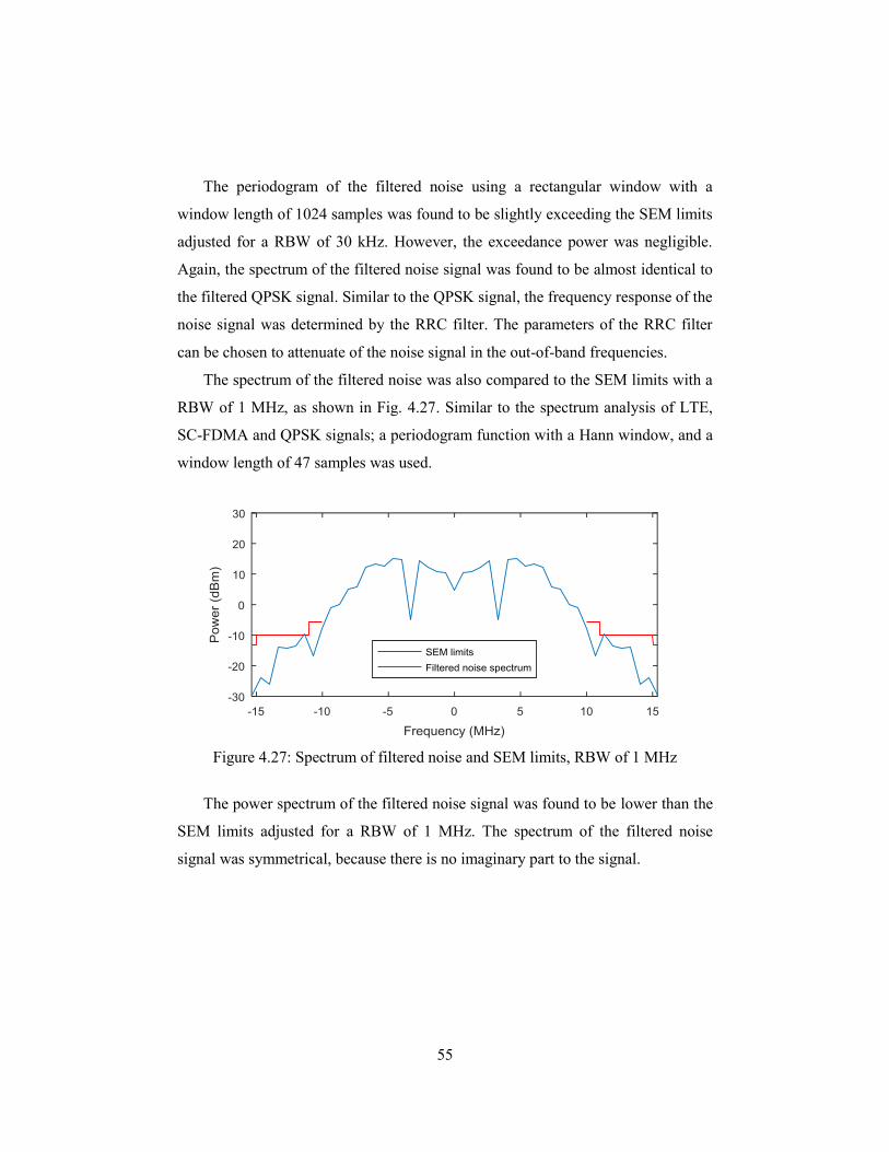
55
The periodogram of the filtered noise using a rectangular window with a
window length of 1024 samples was found to be slightly exceeding the SEM limits
adjusted for a RBW of 30 kHz. However, the exceedance power was negligible.
Again, the spectrum of the filtered noise signal was found to be almost identical to
the filtered QPSK signal. Similar to the QPSK signal, the frequency response of the
noise signal was determined by the RRC filter. The parameters of the RRC filter
can be chosen to attenuate of the noise signal in the out-of-band frequencies.
The spectrum of the filtered noise was also compared to the SEM limits with a
RBW of 1 MHz, as shown in Fig. 4.27. Similar to the spectrum analysis of LTE,
SC-FDMA and QPSK signals; a periodogram function with a Hann window, and a
window length of 47 samples was used.
Figure 4.27: Spectrum of filtered noise and SEM limits, RBW of 1 MHz
The power spectrum of the filtered noise signal was found to be lower than the
SEM limits adjusted for a RBW of 1 MHz. The spectrum of the filtered noise
signal was symmetrical, because there is no imaginary part to the signal.
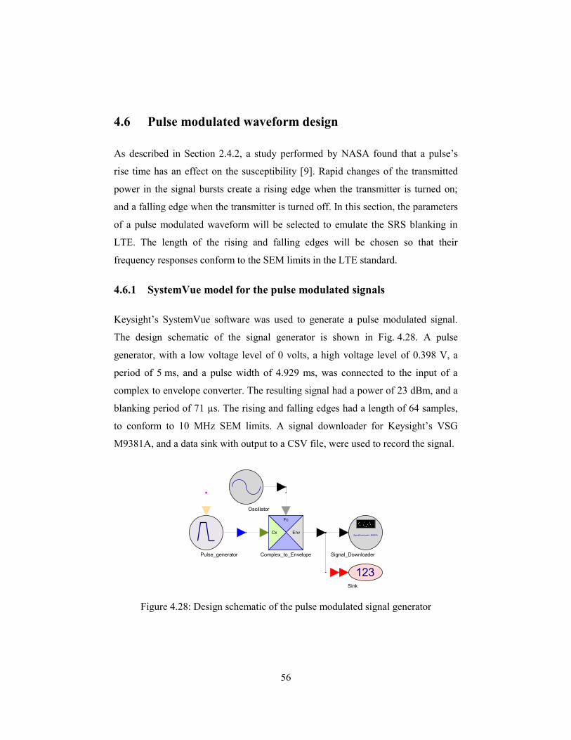
56
4.6 Pulse modulated waveform design
As described in Section 2.4.2, a study performed by NASA found that a pulse’s
rise time has an effect on the susceptibility [9]. Rapid changes of the transmitted
power in the signal bursts create a rising edge when the transmitter is turned on;
and a falling edge when the transmitter is turned off. In this section, the parameters
of a pulse modulated waveform will be selected to emulate the SRS blanking in
LTE. The length of the rising and falling edges will be chosen so that their
frequency responses conform to the SEM limits in the LTE standard.
4.6.1 SystemVue model for the pulse modulated signals
Keysight’s SystemVue software was used to generate a pulse modulated signal.
The design schematic of the signal generator is shown in Fig. 4.28. A pulse
generator, with a low voltage level of 0 volts, a high voltage level of 0.398 V, a
period of 5 ms, and a pulse width of 4.929 ms, was connected to the input of a
complex to envelope converter. The resulting signal had a power of 23 dBm, and a
blanking period of 71 µs. The rising and falling edges had a length of 64 samples,
to conform to 10 MHz SEM limits. A signal downloader for Keysight’s VSG
M9381A, and a data sink with output to a CSV file, were used to record the signal.
Figure 4.28: Design schematic of the pulse modulated signal generator
Oscillator
Fc
EnvCx
Complex_to_EnvelopePulse_generator
123Sink
SignalDownloader_M9381A
Signal_Downloader
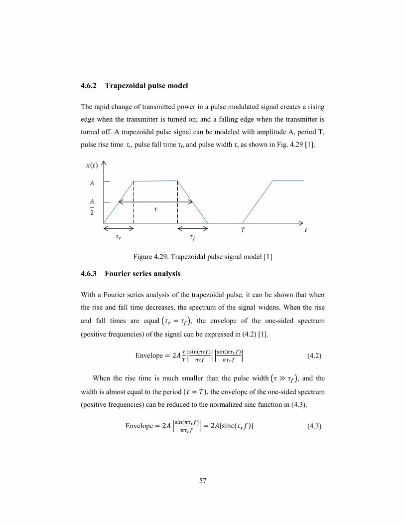
57
4.6.2 Trapezoidal pulse model
The rapid change of transmitted power in a pulse modulated signal creates a rising
edge when the transmitter is turned on; and a falling edge when the transmitter is
turned off. A trapezoidal pulse signal can be modeled with amplitude A, period T,
pulse rise time τr, pulse fall time τf, and pulse width τ, as shown in Fig. 4.29 [1].
Figure 4.29: Trapezoidal pulse signal model [1]
4.6.3 Fourier series analysis
With a Fourier series analysis of the trapezoidal pulse, it can be shown that when
the rise and fall time decreases, the spectrum of the signal widens. When the rise
and fall times are equal ( ), the envelope of the one-sided spectrum
(positive frequencies) of the signal can be expressed in (4.2) [1].
Envelope
| ( )
| | ( )
| (4.2)
When the rise time is much smaller than the pulse width ( ), and the
width is almost equal to the period ( ), the envelope of the one-sided spectrum
(positive frequencies) can be reduced to the normalized sinc function in (4.3).
Envelope | ( )
| | ( )| (4.3)
( )
t
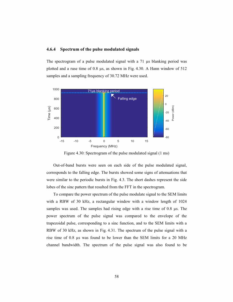
58
4.6.4 Spectrum of the pulse modulated signals
The spectrogram of a pulse modulated signal with a 71 µs blanking period was
plotted and a ruse time of 0.8 µs, as shown in Fig. 4.30. A Hann window of 512
samples and a sampling frequency of 30.72 MHz were used.
Figure 4.30: Spectrogram of the pulse modulated signal (1 ms)
Out-of-band bursts were seen on each side of the pulse modulated signal,
corresponds to the falling edge. The bursts showed some signs of attenuations that
were similar to the periodic bursts in Fig. 4.3. The short dashes represent the side
lobes of the sinc pattern that resulted from the FFT in the spectrogram.
To compare the power spectrum of the pulse modulate signal to the SEM limits
with a RBW of 30 kHz, a rectangular window with a window length of 1024
samples was used. The samples had rising edge with a rise time of 0.8 µs. The
power spectrum of the pulse signal was compared to the envelope of the
trapezoidal pulse, corresponding to a sinc function, and to the SEM limits with a
RBW of 30 kHz, as shown in Fig. 4.31. The spectrum of the pulse signal with a
rise time of 0.8 µs was found to be lower than the SEM limits for a 20 MHz
channel bandwidth. The spectrum of the pulse signal was also found to be
71µs blanking period
Falling edge
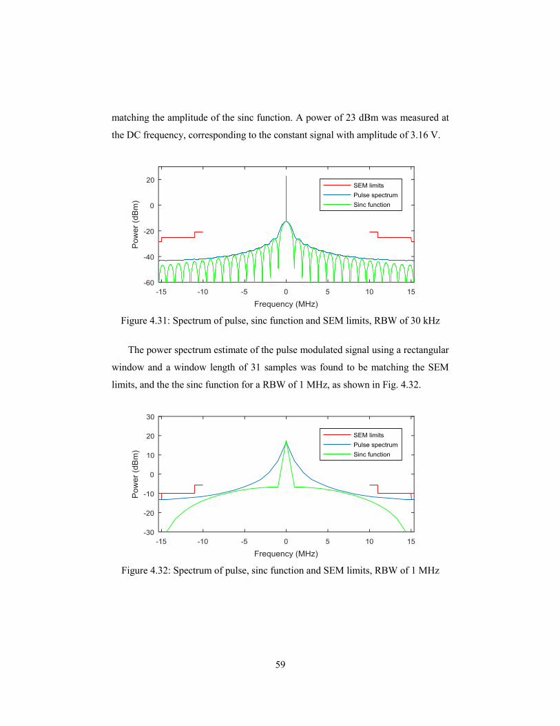
59
matching the amplitude of the sinc function. A power of 23 dBm was measured at
the DC frequency, corresponding to the constant signal with amplitude of 3.16 V.
Figure 4.31: Spectrum of pulse, sinc function and SEM limits, RBW of 30 kHz
The power spectrum estimate of the pulse modulated signal using a rectangular
window and a window length of 31 samples was found to be matching the SEM
limits, and the the sinc function for a RBW of 1 MHz, as shown in Fig. 4.32.
Figure 4.32: Spectrum of pulse, sinc function and SEM limits, RBW of 1 MHz
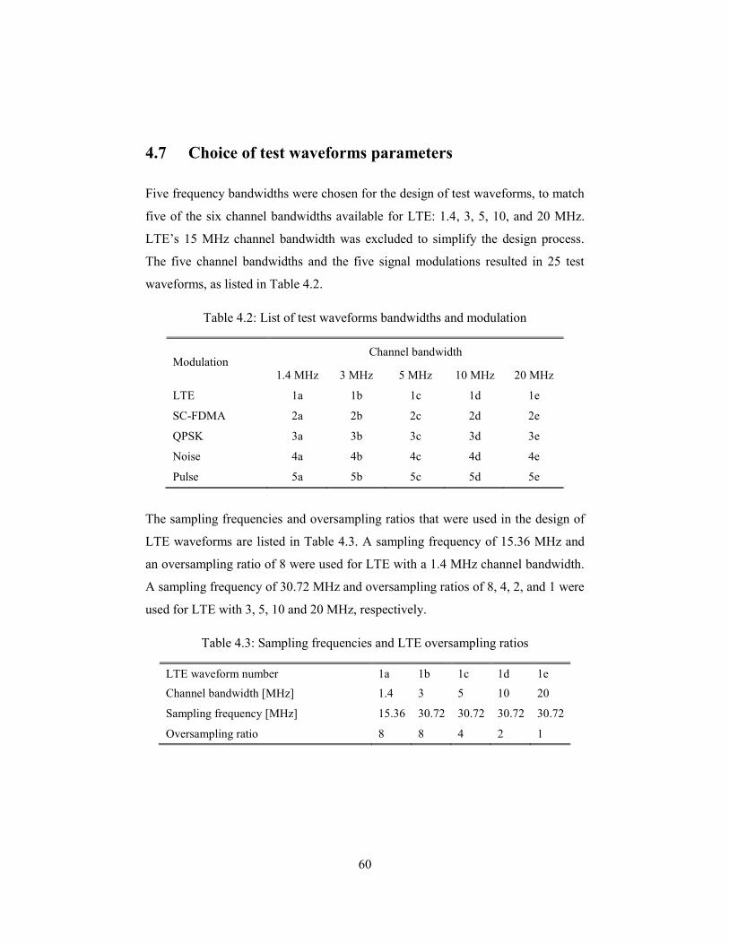
60
4.7 Choice of test waveforms parameters
Five frequency bandwidths were chosen for the design of test waveforms, to match
five of the six channel bandwidths available for LTE: 1.4, 3, 5, 10, and 20 MHz.
LTE’s 15 MHz channel bandwidth was excluded to simplify the design process.
The five channel bandwidths and the five signal modulations resulted in 25 test
waveforms, as listed in Table 4.2.
Table 4.2: List of test waveforms bandwidths and modulation
Modulation Channel bandwidth
1.4 MHz 3 MHz 5 MHz 10 MHz 20 MHz
LTE 1a 1b 1c 1d 1e
SC-FDMA 2a 2b 2c 2d 2e
QPSK 3a 3b 3c 3d 3e
Noise 4a 4b 4c 4d 4e
Pulse 5a 5b 5c 5d 5e
The sampling frequencies and oversampling ratios that were used in the design of
LTE waveforms are listed in Table 4.3. A sampling frequency of 15.36 MHz and
an oversampling ratio of 8 were used for LTE with a 1.4 MHz channel bandwidth.
A sampling frequency of 30.72 MHz and oversampling ratios of 8, 4, 2, and 1 were
used for LTE with 3, 5, 10 and 20 MHz, respectively.
Table 4.3: Sampling frequencies and LTE oversampling ratios
LTE waveform number 1a 1b 1c 1d 1e
Channel bandwidth [MHz] 1.4 3 5 10 20
Sampling frequency [MHz] 15.36 30.72 30.72 30.72 30.72
Oversampling ratio 8 8 4 2 1
61
The numbers of subcarriers for SC-FDMA waveforms were chosen to match the
channel bandwidths, as listed in Table 4.4. A FFT length of 2048 samples and a
sampling frequency of 30.72 MHz were used for all SC-FDMA waveforms.
Table 4.4: Maximum number of subcarriers for SC-FDMA
SC-FDMA waveform number 2a 2b 2c 2d 2e
Channel bandwidth [MHz] 1.4 3 5 10 20
Number of subcarriers 72 180 300 600 1200
The upsampling factors in the RRC filters were chosen to match the channel
bandwidths, as listed in Table 4.5. A span of 6 samples, a roll-off factor of 0.22 and
a sampling frequency of 30.72 MHz were used for all filtered waveforms.
Table 4.5: RRC upsampling factors
QPSK/Noise waveform number 3a/4a 3b/4b 3c/4c 3d/4d 3e/4e
Channel bandwidth [MHz] 1.4 3 5 10 20
RRC filter upsampling factor 32 16 8 4 2
The rise times of the pulse modulation were chosen to match the channel
bandwidths, as listed in Table 4.6. A pulse repetition interval of 5 ms and a
sampling frequency of 30.72 MHz were used for all pulse modulated waveforms.
Table 4.6: Rise time and measurement bandwidth of ramp function
Pulse modulated waveform number 5a 5b 5c 5d 5e
Channel bandwidth [MHz] 1.4 3 5 10 20
Rise time [µs] 12.8 6.4 3.2 1.6 0.8
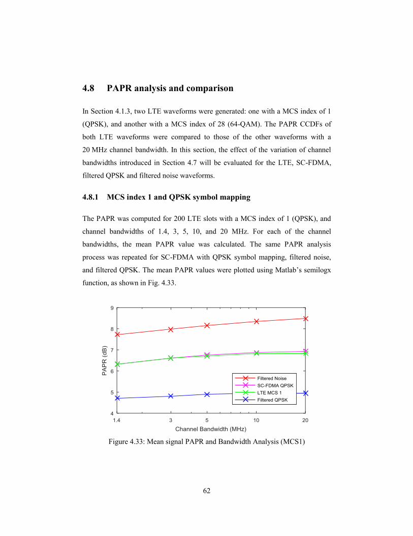
62
4.8 PAPR analysis and comparison
In Section 4.1.3, two LTE waveforms were generated: one with a MCS index of 1
(QPSK), and another with a MCS index of 28 (64-QAM). The PAPR CCDFs of
both LTE waveforms were compared to those of the other waveforms with a
20 MHz channel bandwidth. In this section, the effect of the variation of channel
bandwidths introduced in Section 4.7 will be evaluated for the LTE, SC-FDMA,
filtered QPSK and filtered noise waveforms.
4.8.1 MCS index 1 and QPSK symbol mapping
The PAPR was computed for 200 LTE slots with a MCS index of 1 (QPSK), and
channel bandwidths of 1.4, 3, 5, 10, and 20 MHz. For each of the channel
bandwidths, the mean PAPR value was calculated. The same PAPR analysis
process was repeated for SC-FDMA with QPSK symbol mapping, filtered noise,
and filtered QPSK. The mean PAPR values were plotted using Matlab’s semilogx
function, as shown in Fig. 4.33.
Figure 4.33: Mean signal PAPR and Bandwidth Analysis (MCS1)
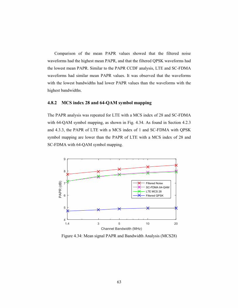
63
Comparison of the mean PAPR values showed that the filtered noise
waveforms had the highest mean PAPR, and that the filtered QPSK waveforms had
the lowest mean PAPR. Similar to the PAPR CCDF analysis, LTE and SC-FDMA
waveforms had similar mean PAPR values. It was observed that the waveforms
with the lowest bandwidths had lower PAPR values than the waveforms with the
highest bandwidths.
4.8.2 MCS index 28 and 64-QAM symbol mapping
The PAPR analysis was repeated for LTE with a MCS index of 28 and SC-FDMA
with 64-QAM symbol mapping, as shown in Fig. 4.34. As found in Section 4.2.3
and 4.3.3, the PAPR of LTE with a MCS index of 1 and SC-FDMA with QPSK
symbol mapping are lower than the PAPR of LTE with a MCS index of 28 and
SC-FDMA with 64-QAM symbol mapping.
Figure 4.34: Mean signal PAPR and Bandwidth Analysis (MCS28)
64
4.9 Summary
Five test waveforms were created using a parameter reduction process: LTE,
SC-FDMA, QPSK, uniform noise, and pulse modulated. Each waveform was
designed for five channel bandwidths: 1.4, 3, 5, 10, and 20 MHz, for a total of 25
test waveforms. The SEM limits were used to set certain parameters of the
waveforms such that their frequency content was similar to each other.
The PAPR of the simulated LTE, SC-FDMA, QPSK, and noise waveforms
were measured. LTE and SC-FDMA waveforms had similar PAPR values. The
PAPR of QPSK waveforms was significantly lower than the PAPR of the noise
waveforms. The QPSK and noise waveforms formed lower and higher bounds for
the PAPR of the LTE and the SC-FDMA waveforms, respectively.
The parameters of the waveforms were carefully selected to ensure a fair
comparison of radiated susceptibility test results. RRC filters with similar
characteristics were used to limit the bandwidth of QPSK and noise waveforms.
The pulse modulated waveform’s repetition interval and duty factor emulated the
SRS blanking in LTE. The lengths of the rising and falling edges were chosen to
match the SEM limits. Finally, the MCS index for LTE and the symbol mapping
for SC-FDMA were chosen to limit the PAPR of those waveforms.
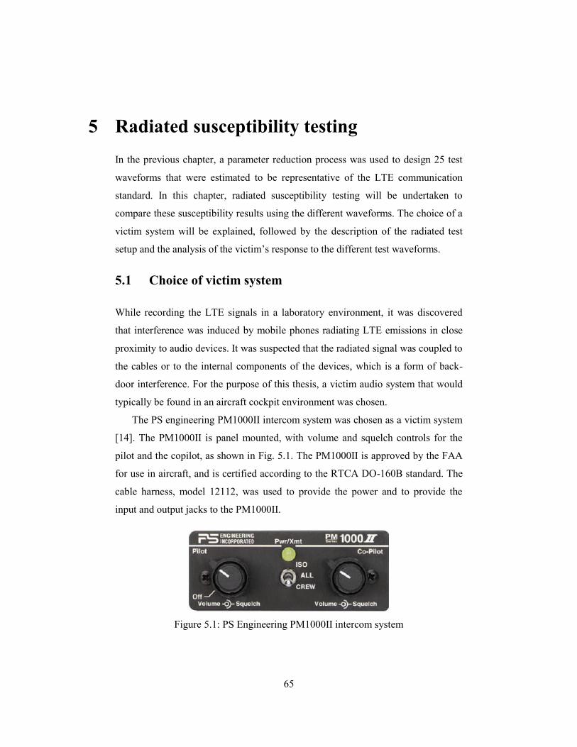
65
5 Radiated susceptibility testing
In the previous chapter, a parameter reduction process was used to design 25 test
waveforms that were estimated to be representative of the LTE communication
standard. In this chapter, radiated susceptibility testing will be undertaken to
compare these susceptibility results using the different waveforms. The choice of a
victim system will be explained, followed by the description of the radiated test
setup and the analysis of the victim’s response to the different test waveforms.
5.1 Choice of victim system
While recording the LTE signals in a laboratory environment, it was discovered
that interference was induced by mobile phones radiating LTE emissions in close
proximity to audio devices. It was suspected that the radiated signal was coupled to
the cables or to the internal components of the devices, which is a form of back-
door interference. For the purpose of this thesis, a victim audio system that would
typically be found in an aircraft cockpit environment was chosen.
The PS engineering PM1000II intercom system was chosen as a victim system
[14]. The PM1000II is panel mounted, with volume and squelch controls for the
pilot and the copilot, as shown in Fig. 5.1. The PM1000II is approved by the FAA
for use in aircraft, and is certified according to the RTCA DO-160B standard. The
cable harness, model 12112, was used to provide the power and to provide the
input and output jacks to the PM1000II.
Figure 5.1: PS Engineering PM1000II intercom system
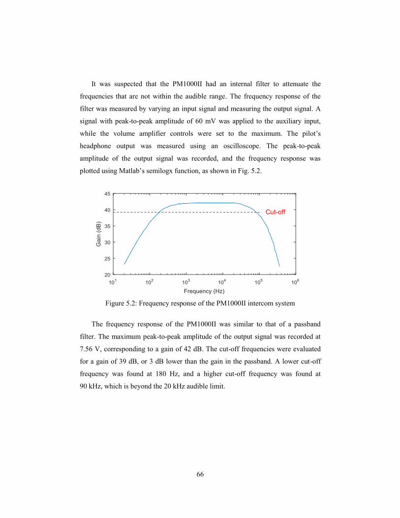
66
It was suspected that the PM1000II had an internal filter to attenuate the
frequencies that are not within the audible range. The frequency response of the
filter was measured by varying an input signal and measuring the output signal. A
signal with peak-to-peak amplitude of 60 mV was applied to the auxiliary input,
while the volume amplifier controls were set to the maximum. The pilot’s
headphone output was measured using an oscilloscope. The peak-to-peak
amplitude of the output signal was recorded, and the frequency response was
plotted using Matlab’s semilogx function, as shown in Fig. 5.2.
Figure 5.2: Frequency response of the PM1000II intercom system
The frequency response of the PM1000II was similar to that of a passband
filter. The maximum peak-to-peak amplitude of the output signal was recorded at
7.56 V, corresponding to a gain of 42 dB. The cut-off frequencies were evaluated
for a gain of 39 dB, or 3 dB lower than the gain in the passband. A lower cut-off
frequency was found at 180 Hz, and a higher cut-off frequency was found at
90 kHz, which is beyond the 20 kHz audible limit.
Cut-off
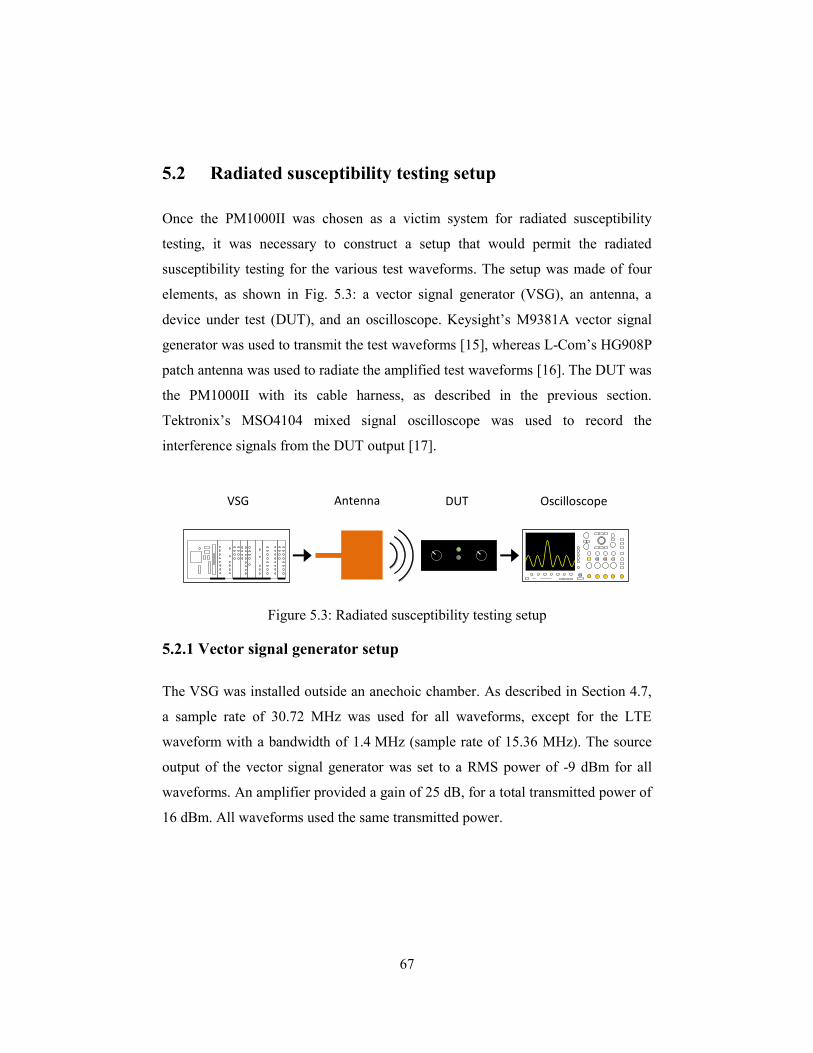
67
5.2 Radiated susceptibility testing setup
Once the PM1000II was chosen as a victim system for radiated susceptibility
testing, it was necessary to construct a setup that would permit the radiated
susceptibility testing for the various test waveforms. The setup was made of four
elements, as shown in Fig. 5.3: a vector signal generator (VSG), an antenna, a
device under test (DUT), and an oscilloscope. Keysight’s M9381A vector signal
generator was used to transmit the test waveforms [15], whereas L-Com’s HG908P
patch antenna was used to radiate the amplified test waveforms [16]. The DUT was
the PM1000II with its cable harness, as described in the previous section.
Tektronix’s MSO4104 mixed signal oscilloscope was used to record the
interference signals from the DUT output [17].
Figure 5.3: Radiated susceptibility testing setup
5.2.1 Vector signal generator setup
The VSG was installed outside an anechoic chamber. As described in Section 4.7,
a sample rate of 30.72 MHz was used for all waveforms, except for the LTE
waveform with a bandwidth of 1.4 MHz (sample rate of 15.36 MHz). The source
output of the vector signal generator was set to a RMS power of -9 dBm for all
waveforms. An amplifier provided a gain of 25 dB, for a total transmitted power of
16 dBm. All waveforms used the same transmitted power.
VSG Antenna DUT Oscilloscope

68
5.2.2 Antenna and DUT setup
The antenna and the DUT were installed in an anechoic chamber, as shown in
Fig. 5.4. The DUT was positioned in close proximity to the antenna. It was found
that the position that yielded the highest coupling was when the connector of the
cable harness was aligned on the center of the antenna. The cable harness of the
PM1000II and the cable of the antenna were kept in the same position to ensure
that the coupling did not vary during radiated susceptibility testing. The enclosure
of the PM1000II was not grounded. The volume amplifier controls were set to the
maximum, and the squelch controls were set to the minimum in order to produce
the highest level of interference.
Figure 5.4: Antenna and DUT setup in the anechoic chamber
5.2.3 Oscilloscope setup
The oscilloscope was installed outside the anechoic chamber. The cable for the
pilot headphone output of the PM1000II was connected to the Tektronix MSO
4104 oscilloscope. A sampling frequency of 5 million samples per second and a
recording of one million samples were used, for a recording length of 200 ms. A
DC coupling and an impedance of 50 ohms were used.
Antenna
DUT
Support structure
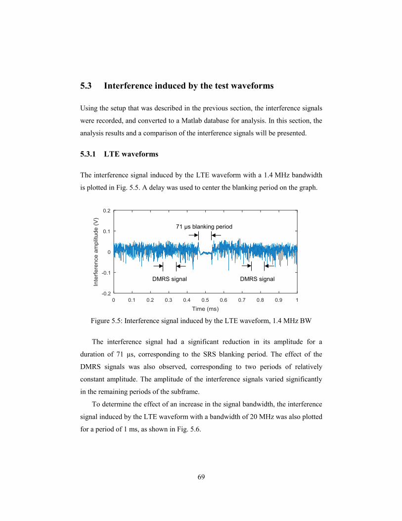
69
5.3 Interference induced by the test waveforms
Using the setup that was described in the previous section, the interference signals
were recorded, and converted to a Matlab database for analysis. In this section, the
analysis results and a comparison of the interference signals will be presented.
5.3.1 LTE waveforms
The interference signal induced by the LTE waveform with a 1.4 MHz bandwidth
is plotted in Fig. 5.5. A delay was used to center the blanking period on the graph.
Figure 5.5: Interference signal induced by the LTE waveform, 1.4 MHz BW
The interference signal had a significant reduction in its amplitude for a
duration of 71 µs, corresponding to the SRS blanking period. The effect of the
DMRS signals was also observed, corresponding to two periods of relatively
constant amplitude. The amplitude of the interference signals varied significantly
in the remaining periods of the subframe.
To determine the effect of an increase in the signal bandwidth, the interference
signal induced by the LTE waveform with a bandwidth of 20 MHz was also plotted
for a period of 1 ms, as shown in Fig. 5.6.
71 µs blanking period
DMRS signal DMRS signal
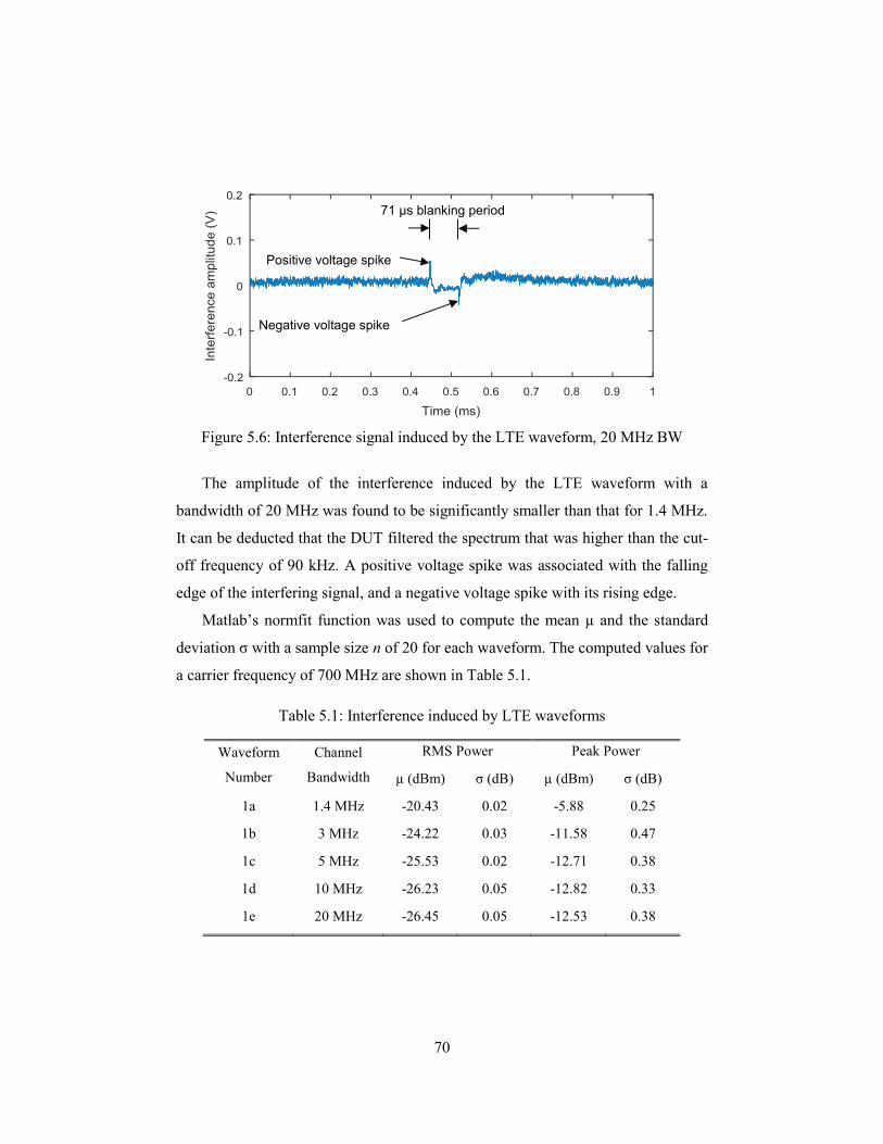
70
Figure 5.6: Interference signal induced by the LTE waveform, 20 MHz BW
The amplitude of the interference induced by the LTE waveform with a
bandwidth of 20 MHz was found to be significantly smaller than that for 1.4 MHz.
It can be deducted that the DUT filtered the spectrum that was higher than the cut-
off frequency of 90 kHz. A positive voltage spike was associated with the falling
edge of the interfering signal, and a negative voltage spike with its rising edge.
Matlab’s normfit function was used to compute the mean µ and the standard
deviation σ with a sample size n of 20 for each waveform. The computed values for
a carrier frequency of 700 MHz are shown in Table 5.1.
Table 5.1: Interference induced by LTE waveforms
Waveform
Number
Channel
Bandwidth
RMS Power Peak Power
µ (dBm) σ (dB) µ (dBm) σ (dB)
1a 1.4 MHz -20.43 0.02 -5.88 0.25
1b 3 MHz -24.22 0.03 -11.58 0.47
1c 5 MHz -25.53 0.02 -12.71 0.38
1d 10 MHz -26.23 0.05 -12.82 0.33
1e 20 MHz -26.45 0.05 -12.53 0.38
71 µs blanking period
Positive voltage spike
Negative voltage spike
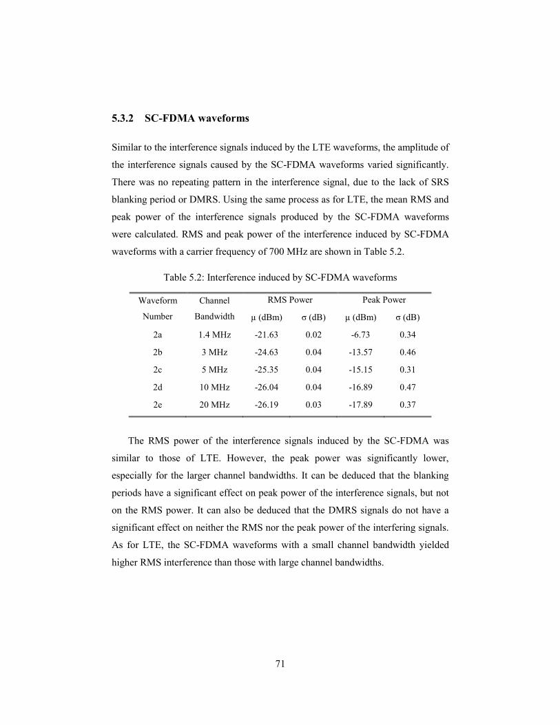
71
5.3.2 SC-FDMA waveforms
Similar to the interference signals induced by the LTE waveforms, the amplitude of
the interference signals caused by the SC-FDMA waveforms varied significantly.
There was no repeating pattern in the interference signal, due to the lack of SRS
blanking period or DMRS. Using the same process as for LTE, the mean RMS and
peak power of the interference signals produced by the SC-FDMA waveforms
were calculated. RMS and peak power of the interference induced by SC-FDMA
waveforms with a carrier frequency of 700 MHz are shown in Table 5.2.
Table 5.2: Interference induced by SC-FDMA waveforms
Waveform
Number
Channel
Bandwidth
RMS Power Peak Power
µ (dBm) σ (dB) µ (dBm) σ (dB)
2a 1.4 MHz -21.63 0.02 -6.73 0.34
2b 3 MHz -24.63 0.04 -13.57 0.46
2c 5 MHz -25.35 0.04 -15.15 0.31
2d 10 MHz -26.04 0.04 -16.89 0.47
2e 20 MHz -26.19 0.03 -17.89 0.37
The RMS power of the interference signals induced by the SC-FDMA was
similar to those of LTE. However, the peak power was significantly lower,
especially for the larger channel bandwidths. It can be deduced that the blanking
periods have a significant effect on peak power of the interference signals, but not
on the RMS power. It can also be deduced that the DMRS signals do not have a
significant effect on neither the RMS nor the peak power of the interfering signals.
As for LTE, the SC-FDMA waveforms with a small channel bandwidth yielded
higher RMS interference than those with large channel bandwidths.
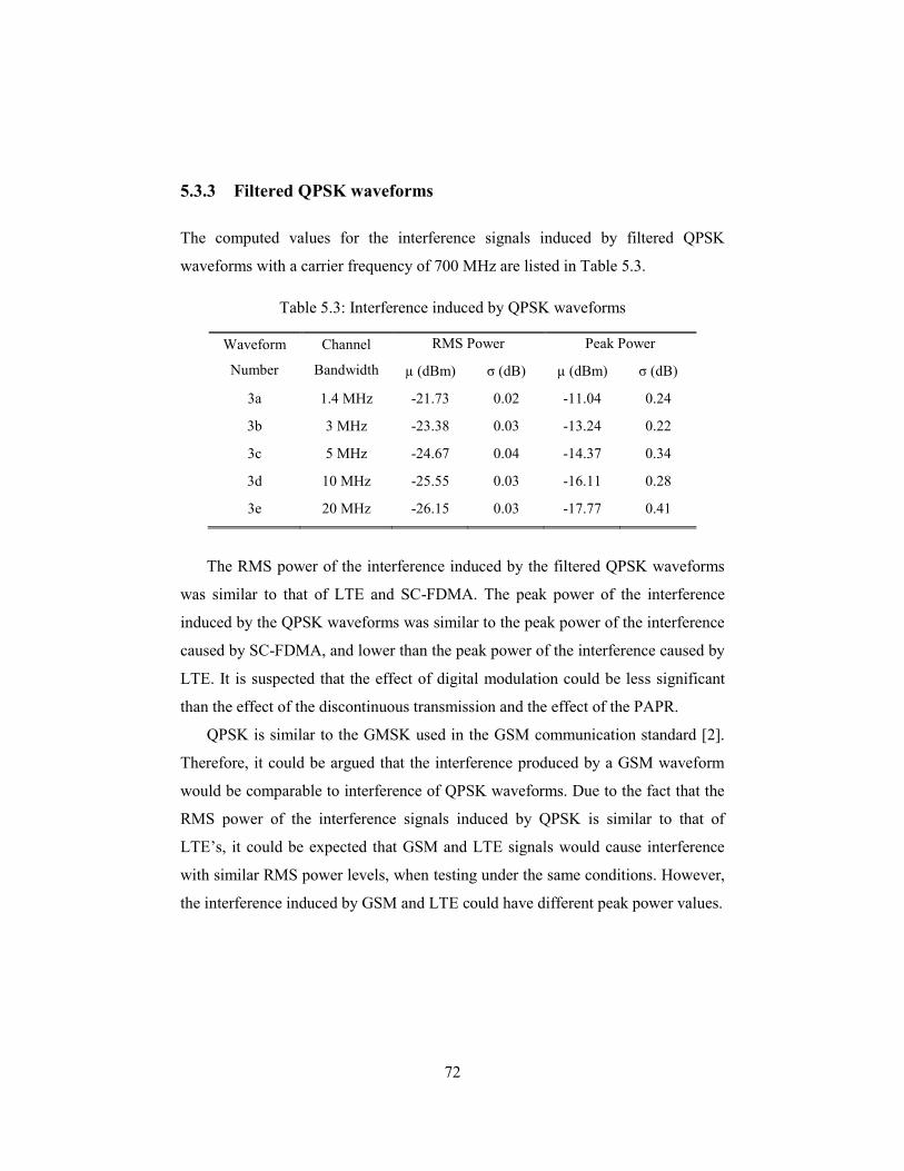
72
5.3.3 Filtered QPSK waveforms
The computed values for the interference signals induced by filtered QPSK
waveforms with a carrier frequency of 700 MHz are listed in Table 5.3.
Table 5.3: Interference induced by QPSK waveforms
Waveform
Number
Channel
Bandwidth
RMS Power Peak Power
µ (dBm) σ (dB) µ (dBm) σ (dB)
3a 1.4 MHz -21.73 0.02 -11.04 0.24
3b 3 MHz -23.38 0.03 -13.24 0.22
3c 5 MHz -24.67 0.04 -14.37 0.34
3d 10 MHz -25.55 0.03 -16.11 0.28
3e 20 MHz -26.15 0.03 -17.77 0.41
The RMS power of the interference induced by the filtered QPSK waveforms
was similar to that of LTE and SC-FDMA. The peak power of the interference
induced by the QPSK waveforms was similar to the peak power of the interference
caused by SC-FDMA, and lower than the peak power of the interference caused by
LTE. It is suspected that the effect of digital modulation could be less significant
than the effect of the discontinuous transmission and the effect of the PAPR.
QPSK is similar to the GMSK used in the GSM communication standard [2].
Therefore, it could be argued that the interference produced by a GSM waveform
would be comparable to interference of QPSK waveforms. Due to the fact that the
RMS power of the interference signals induced by QPSK is similar to that of
LTE’s, it could be expected that GSM and LTE signals would cause interference
with similar RMS power levels, when testing under the same conditions. However,
the interference induced by GSM and LTE could have different peak power values.
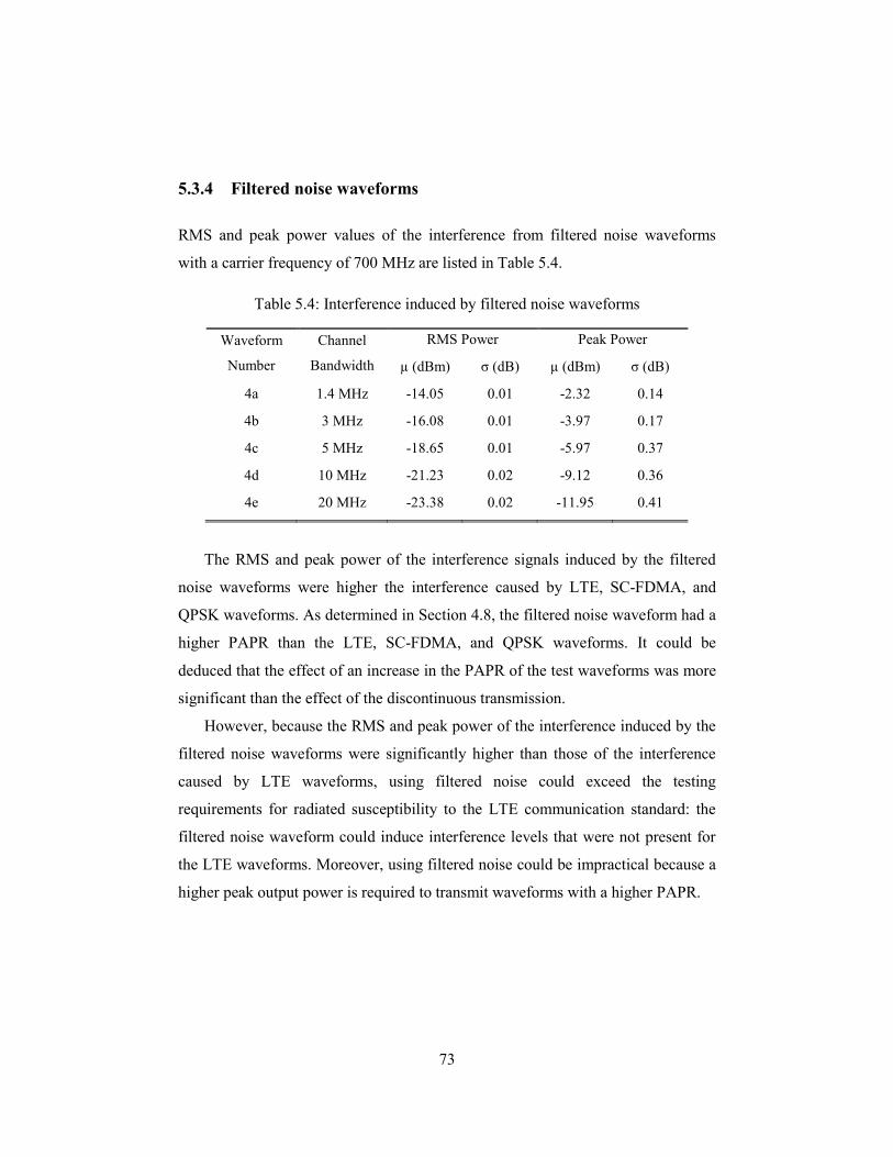
73
5.3.4 Filtered noise waveforms
RMS and peak power values of the interference from filtered noise waveforms
with a carrier frequency of 700 MHz are listed in Table 5.4.
Table 5.4: Interference induced by filtered noise waveforms
Waveform
Number
Channel
Bandwidth
RMS Power Peak Power
µ (dBm) σ (dB) µ (dBm) σ (dB)
4a 1.4 MHz -14.05 0.01 -2.32 0.14
4b 3 MHz -16.08 0.01 -3.97 0.17
4c 5 MHz -18.65 0.01 -5.97 0.37
4d 10 MHz -21.23 0.02 -9.12 0.36
4e 20 MHz -23.38 0.02 -11.95 0.41
The RMS and peak power of the interference signals induced by the filtered
noise waveforms were higher the interference caused by LTE, SC-FDMA, and
QPSK waveforms. As determined in Section 4.8, the filtered noise waveform had a
higher PAPR than the LTE, SC-FDMA, and QPSK waveforms. It could be
deduced that the effect of an increase in the PAPR of the test waveforms was more
significant than the effect of the discontinuous transmission.
However, because the RMS and peak power of the interference induced by the
filtered noise waveforms were significantly higher than those of the interference
caused by LTE waveforms, using filtered noise could exceed the testing
requirements for radiated susceptibility to the LTE communication standard: the
filtered noise waveform could induce interference levels that were not present for
the LTE waveforms. Moreover, using filtered noise could be impractical because a
higher peak output power is required to transmit waveforms with a higher PAPR.
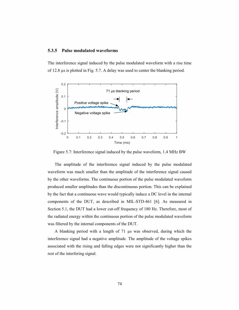
74
5.3.5 Pulse modulated waveforms
The interference signal induced by the pulse modulated waveform with a rise time
of 12.8 µs is plotted in Fig. 5.7. A delay was used to center the blanking period.
Figure 5.7: Interference signal induced by the pulse waveform, 1.4 MHz BW
The amplitude of the interference signal induced by the pulse modulated
waveform was much smaller than the amplitude of the interference signal caused
by the other waveforms. The continuous portion of the pulse modulated waveform
produced smaller amplitudes than the discontinuous portion. This can be explained
by the fact that a continuous wave would typically induce a DC level in the internal
components of the DUT, as described in MIL-STD-461 [6]. As measured in
Section 5.1, the DUT had a lower cut-off frequency of 180 Hz. Therefore, most of
the radiated energy within the continuous portion of the pulse modulated waveform
was filtered by the internal components of the DUT.
A blanking period with a length of 71 µs was observed, during which the
interference signal had a negative amplitude. The amplitude of the voltage spikes
associated with the rising and falling edges were not significantly higher than the
rest of the interfering signal.
71 µs blanking period
Positive voltage spike
Negative voltage spike
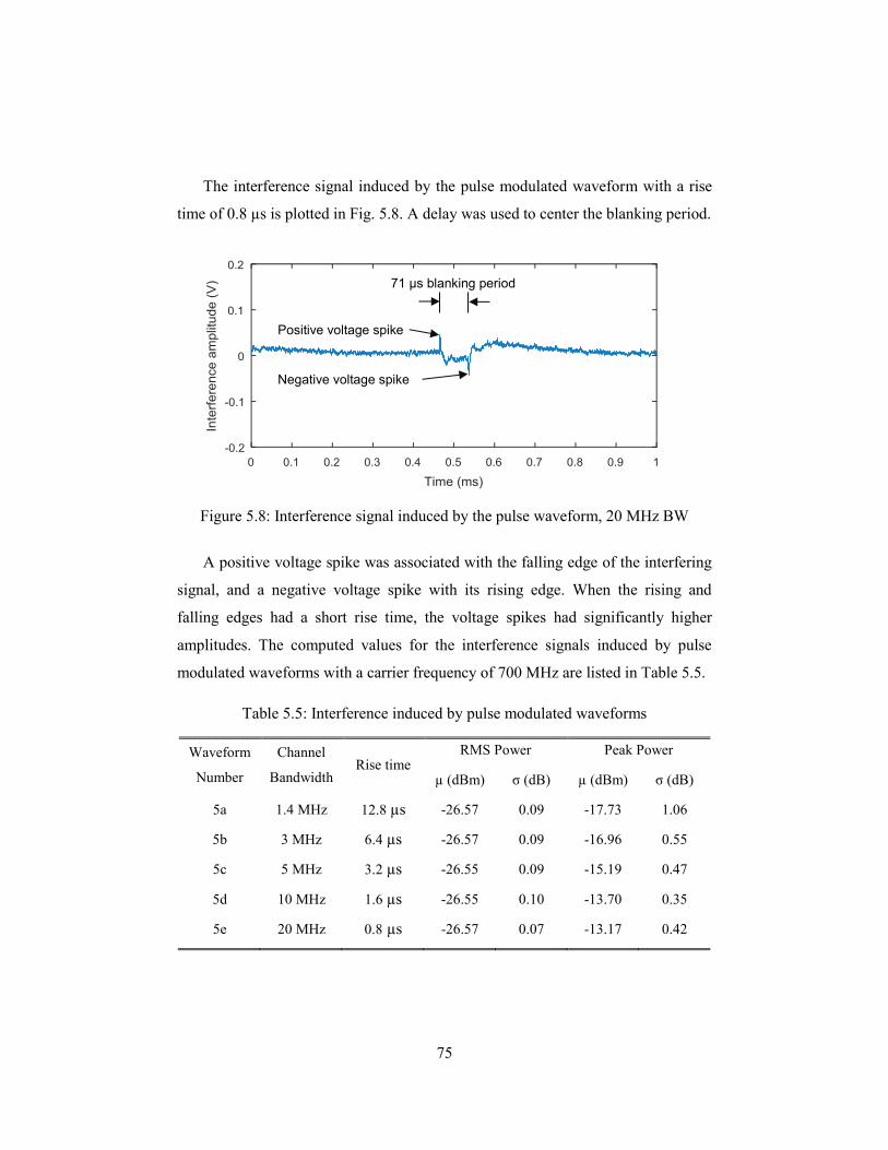
75
The interference signal induced by the pulse modulated waveform with a rise
time of 0.8 µs is plotted in Fig. 5.8. A delay was used to center the blanking period.
Figure 5.8: Interference signal induced by the pulse waveform, 20 MHz BW
A positive voltage spike was associated with the falling edge of the interfering
signal, and a negative voltage spike with its rising edge. When the rising and
falling edges had a short rise time, the voltage spikes had significantly higher
amplitudes. The computed values for the interference signals induced by pulse
modulated waveforms with a carrier frequency of 700 MHz are listed in Table 5.5.
Table 5.5: Interference induced by pulse modulated waveforms
Waveform
Number
Channel
Bandwidth Rise time
RMS Power Peak Power
µ (dBm) σ (dB) µ (dBm) σ (dB)
5a 1.4 MHz 12.8 µs -26.57 0.09 -17.73 1.06
5b 3 MHz 6.4 µs -26.57 0.09 -16.96 0.55
5c 5 MHz 3.2 µs -26.55 0.09 -15.19 0.47
5d 10 MHz 1.6 µs -26.55 0.10 -13.70 0.35
5e 20 MHz 0.8 µs -26.57 0.07 -13.17 0.42
71 µs blanking period
Positive voltage spike
Negative voltage spike
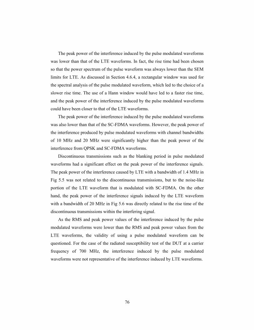
76
The peak power of the interference induced by the pulse modulated waveforms
was lower than that of the LTE waveforms. In fact, the rise time had been chosen
so that the power spectrum of the pulse waveform was always lower than the SEM
limits for LTE. As discussed in Section 4.6.4, a rectangular window was used for
the spectral analysis of the pulse modulated waveform, which led to the choice of a
slower rise time. The use of a Hann window would have led to a faster rise time,
and the peak power of the interference induced by the pulse modulated waveforms
could have been closer to that of the LTE waveforms.
The peak power of the interference induced by the pulse modulated waveforms
was also lower than that of the SC-FDMA waveforms. However, the peak power of
the interference produced by pulse modulated waveforms with channel bandwidths
of 10 MHz and 20 MHz were significantly higher than the peak power of the
interference from QPSK and SC-FDMA waveforms.
Discontinuous transmissions such as the blanking period in pulse modulated
waveforms had a significant effect on the peak power of the interference signals.
The peak power of the interference caused by LTE with a bandwidth of 1.4 MHz in
Fig 5.5 was not related to the discontinuous transmissions, but to the noise-like
portion of the LTE waveform that is modulated with SC-FDMA. On the other
hand, the peak power of the interference signals induced by the LTE waveform
with a bandwidth of 20 MHz in Fig 5.6 was directly related to the rise time of the
discontinuous transmissions within the interfering signal.
As the RMS and peak power values of the interference induced by the pulse
modulated waveforms were lower than the RMS and peak power values from the
LTE waveforms, the validity of using a pulse modulated waveform can be
questioned. For the case of the radiated susceptibility test of the DUT at a carrier
frequency of 700 MHz, the interference induced by the pulse modulated
waveforms were not representative of the interference induced by LTE waveforms.
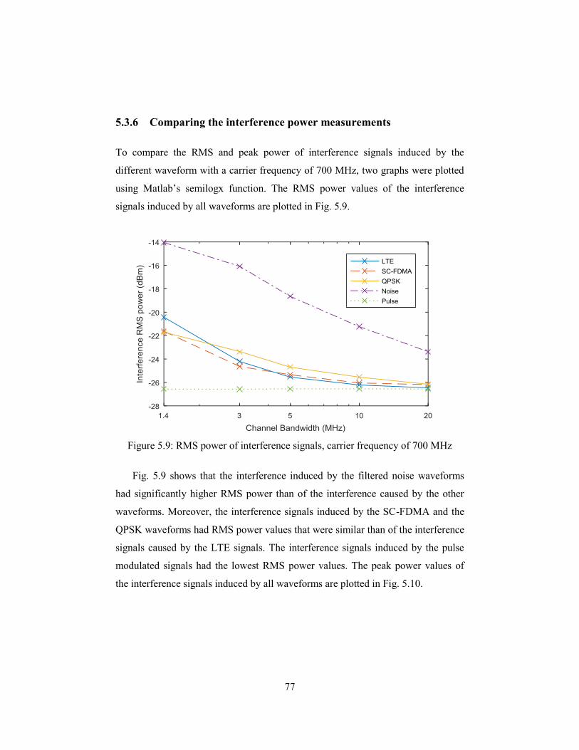
77
5.3.6 Comparing the interference power measurements
To compare the RMS and peak power of interference signals induced by the
different waveform with a carrier frequency of 700 MHz, two graphs were plotted
using Matlab’s semilogx function. The RMS power values of the interference
signals induced by all waveforms are plotted in Fig. 5.9.
Figure 5.9: RMS power of interference signals, carrier frequency of 700 MHz
Fig. 5.9 shows that the interference induced by the filtered noise waveforms
had significantly higher RMS power than of the interference caused by the other
waveforms. Moreover, the interference signals induced by the SC-FDMA and the
QPSK waveforms had RMS power values that were similar than of the interference
signals caused by the LTE signals. The interference signals induced by the pulse
modulated signals had the lowest RMS power values. The peak power values of
the interference signals induced by all waveforms are plotted in Fig. 5.10.
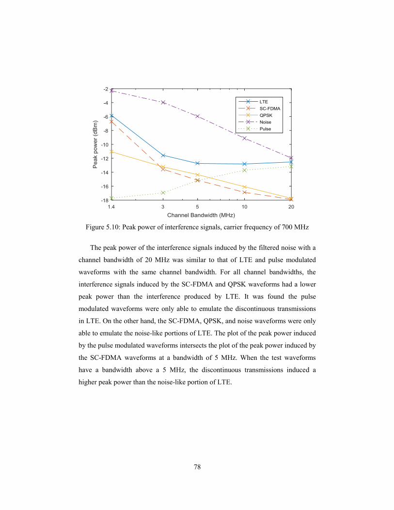
78
Figure 5.10: Peak power of interference signals, carrier frequency of 700 MHz
The peak power of the interference signals induced by the filtered noise with a
channel bandwidth of 20 MHz was similar to that of LTE and pulse modulated
waveforms with the same channel bandwidth. For all channel bandwidths, the
interference signals induced by the SC-FDMA and QPSK waveforms had a lower
peak power than the interference produced by LTE. It was found the pulse
modulated waveforms were only able to emulate the discontinuous transmissions
in LTE. On the other hand, the SC-FDMA, QPSK, and noise waveforms were only
able to emulate the noise-like portions of LTE. The plot of the peak power induced
by the pulse modulated waveforms intersects the plot of the peak power induced by
the SC-FDMA waveforms at a bandwidth of 5 MHz. When the test waveforms
have a bandwidth above a 5 MHz, the discontinuous transmissions induced a
higher peak power than the noise-like portion of LTE.
79
5.3.7 Sweeping carrier frequencies
To observe the effect of a change of the carrier frequency in the test waveforms,
carrier frequencies from 700 MHz to 960 MHz were used, corresponding to the
lowest band of frequencies allocated for LTE [3]. The frequencies were swept in
increments of 10 MHz, resulting in a total of 27 frequency values. The RMS power
values of the interference signals induced by waveforms with a channel bandwidth
of 1.4 MHz are plotted in Fig. 5.11.
Figure 5.11: RMS power of interference signals, 1.4 MHz BW
The observations made with a carrier frequency of 700 MHz were valid for all
other carrier frequencies: the filtered noise induced the highest RMS power; pulse
modulated waveforms induced the lowest RMS power; LTE, SC-FDMA and
QPSK induced a similar RMS power.
The RMS power values of the interference signals induced by waveforms with
a channel bandwidth of 20 MHz are plotted in Fig. 5.12. The limits of the y axis
were modified to improve the visibility of the traces.
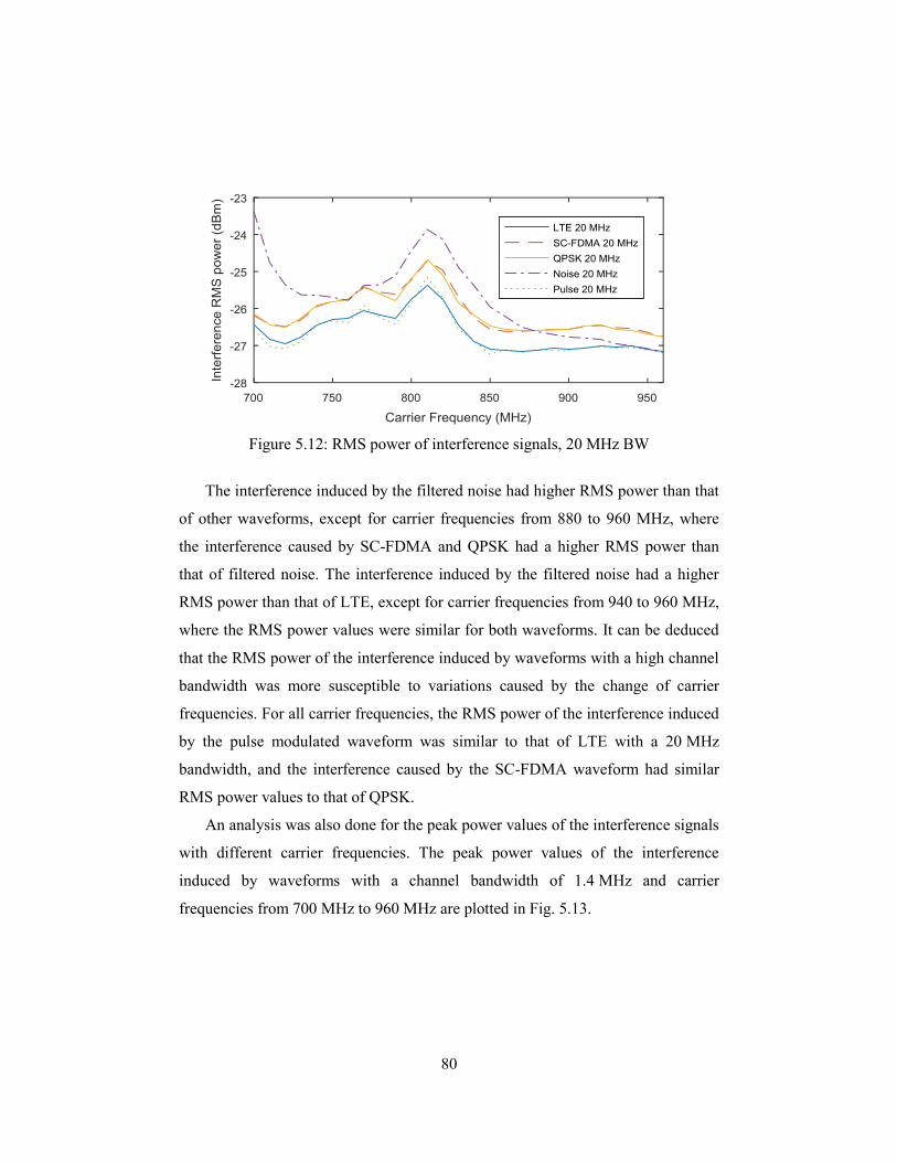
80
Figure 5.12: RMS power of interference signals, 20 MHz BW
The interference induced by the filtered noise had higher RMS power than that
of other waveforms, except for carrier frequencies from 880 to 960 MHz, where
the interference caused by SC-FDMA and QPSK had a higher RMS power than
that of filtered noise. The interference induced by the filtered noise had a higher
RMS power than that of LTE, except for carrier frequencies from 940 to 960 MHz,
where the RMS power values were similar for both waveforms. It can be deduced
that the RMS power of the interference induced by waveforms with a high channel
bandwidth was more susceptible to variations caused by the change of carrier
frequencies. For all carrier frequencies, the RMS power of the interference induced
by the pulse modulated waveform was similar to that of LTE with a 20 MHz
bandwidth, and the interference caused by the SC-FDMA waveform had similar
RMS power values to that of QPSK.
An analysis was also done for the peak power values of the interference signals
with different carrier frequencies. The peak power values of the interference
induced by waveforms with a channel bandwidth of 1.4 MHz and carrier
frequencies from 700 MHz to 960 MHz are plotted in Fig. 5.13.
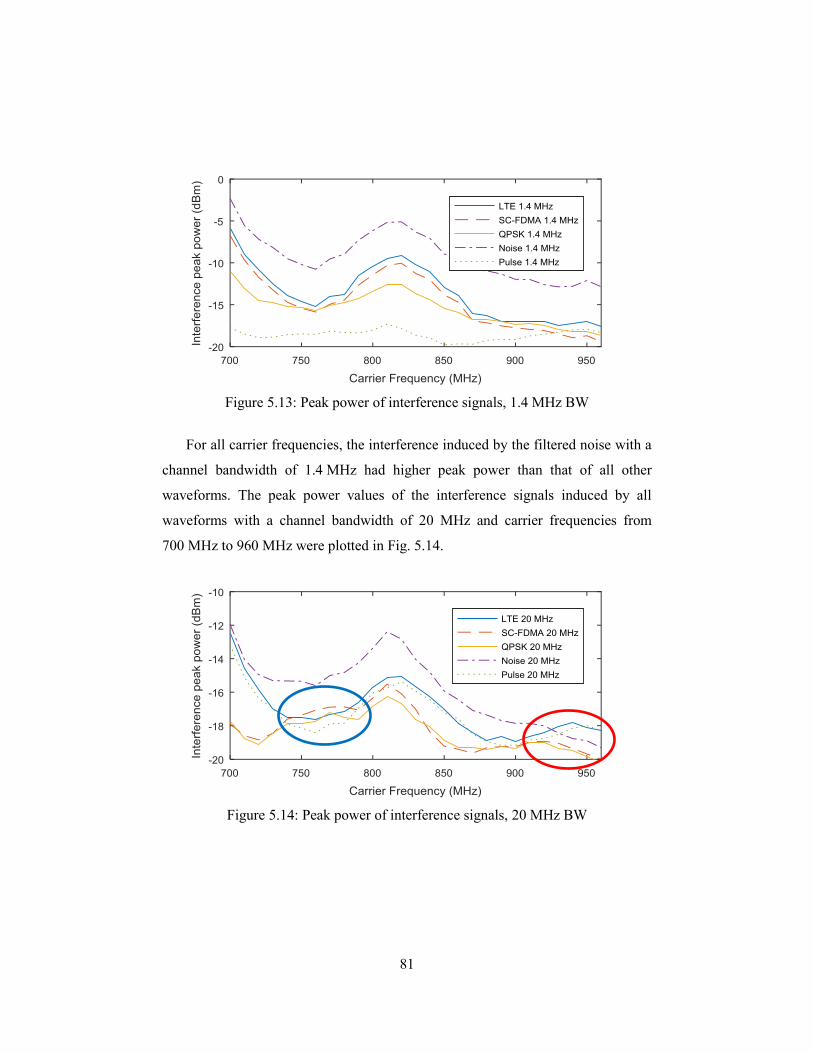
81
Figure 5.13: Peak power of interference signals, 1.4 MHz BW
For all carrier frequencies, the interference induced by the filtered noise with a
channel bandwidth of 1.4 MHz had higher peak power than that of all other
waveforms. The peak power values of the interference signals induced by all
waveforms with a channel bandwidth of 20 MHz and carrier frequencies from
700 MHz to 960 MHz were plotted in Fig. 5.14.
Figure 5.14: Peak power of interference signals, 20 MHz BW
82
The interference induced by the noise waveform had a higher peak power than
that of all other waveforms, except for carrier frequencies from 920 to 960 MHz, as
highlighted by the red circle. The interference produced by the LTE and pulse
modulated waveforms had a higher peak power than that of SC-FDMA and QPSK,
except for carrier frequencies from 740 to 790 MHz, as highlighted by the blue
circle. The effect of the discontinuous transmission on the peak power was more
significant for waveforms with higher channel bandwidths.
It was observed that, only when the bandwidth of a LTE waveform is much
wider than the passband of the DUT, the interference induced by a pulse modulated
waveform were representative of the interference caused by the LTE waveform.
When the bandwidths of the test waveforms were smaller than 10 MHz, the
SC-FDMA, QPSK, and filtered noise waveforms provided better representation of
the interference produced by LTE than the pulse modulated waveform.
These observations did not validate the claim by the DO294C that the highest
interference threat is linked to pulse modulation [4]. Waveforms with a high PAPR
such as the filtered noise induced interference signals with significantly higher
RMS and peak power values, especially for narrow channel bandwidths.
As the RMS and peak power of the interference induced by filtered noise with
a channel bandwidth of 1.4 MHz were always higher than that of LTE, filtered
noise with a small bandwidth could be adequate for radiated susceptibility testing:
they over-estimate the amplitude variations of the LTE signals. If no radiated
susceptibilities were found using a filtered noise waveform, the immunity to the
LTE standard could be determined. Besides, noise waveforms could exceed the
radiated susceptibility testing requirements for LTE: the filtered noise waveform
could induce interference levels that were not present for the LTE waveforms.
83
5.4 Summary
Radiated susceptibility testing was used to compare the interference signals
induced from the test waveforms that were previously designed. The PM1000II
was chosen as a victim system, and its frequency response was evaluated.
It was found that discontinuous transmissions such as the blanking periods in
LTE and in the pulse modulated waveforms have a significant effect on the peak
power of the interference signals. In this case, continuous waveforms such as
SC-FDMA with a similar PAPR to that of LTE, could not emulate the effects of
discontinuous waveforms during radiated susceptibility testing. When bandwidth is
increased, the effect of the discontinuous transmission on the peak power becomes
more significant.
It was also found that the effect on the interference of an increase in the PAPR
of the test waveforms was more significant than the effect of the discontinuous
transmission. The RMS and peak power of the interference induced by the filtered
noise waveforms were significantly higher than those of the interference from
LTE. The use of filtered noise waveforms for radiated susceptibility testing is
relevant.
When the bandwidth of a signal is much wider than the passband of the DUT,
the interference induced by a pulse modulated waveform could be representative
by a noise-like signal. However, when the bandwidth of the test waveforms was
smaller than 10 MHz, the RMS and peak power values of the interference
produced by the pulse modulated waveforms were significantly lower than that of
LTE. Therefore, the validity of only using a pulse modulated waveform for
radiated susceptibility testing can be rejected.
84
6 Conclusion
6.1 Summary
The EMC standards that were reviewed for the purpose of this thesis were found to
rely heavily on a pulse modulated signal, with parameters that were representative
of the GSM standard. However, previous research on radiated susceptibility testing
showed that complex signals can induce susceptibilities that were not present for
the pulse modulated signal. Different LTE signals were recorded and analyzed: the
analysis showed that the peak power was normally distributed; that the OBW and
the PAPR measurement of a LTE signal were not independent.
LTE, SC-FDMA, QPSK, uniform noise, and pulse modulated waveforms were
designed using a parameter reduction process. The waveforms parameters were set
such that their power spectrum matched the spectrum emission mask of the LTE
standard. LTE and SC-FDMA waveforms had similar PAPR values; QPSK had a
lower PAPR; filtered noise waveforms had a higher PAPR. Radiated susceptibility
testing used the PM1000II intercom system as a victim to compare the interference
signals induced from the different test waveforms, sweeping the carrier frequency
from 700 to 960 MHz.
6.2 Conclusions
The discontinuous transmissions in the LTE and in the pulse modulated
waveforms had a significant effect on the peak power of the interference signals.
However, the effect the PAPR was more significant than the effect of the
discontinuous transmission. In fact, the RMS and peak power of the interference
induced by the filtered noise waveforms were significantly higher than those of all
other waveforms. It is proposed that filtered noise waveforms can be used with
confidence for radiated susceptibility testing.
85
The pulse modulated waveform were only representative of the LTE signal
when the bandwidths of the LTE signals were much wider than the passband of the
DUT. Otherwise, the interference levels produced by the pulse modulated
waveforms were significantly lower than that of LTE. It is concluded that pulse
modulated waveforms cannot be used alone for radiated susceptibility testing.
6.3 Contributions
The most important contribution of this thesis is a set of waveforms parameters that
could be used to simulate the interference effects of the LTE communication
standard. There are three secondary contributions of this thesis. The first is a
method to analyze the parameters of a communication signals to extract the
parameters for radiated susceptibility testing: for the first time, actual LTE signals
were recorded at RMCC. The second is a parameters reduction process to simplify
the testing of complex signals. The third is a method to validate the test signals for
specific communication standards.
6.4 Future Work
Upon the completion of this thesis, the subject related to antennas for EMC
immunity testing was found to require future work. In this thesis, a microstrip
patch antenna was used to emulate the radiation pattern and gain of the planar
inverted F antennas found in mobile devices. However, most patch antennas suffer
from a relatively small bandwidth. It must be determined if microstrip patch
antennas can used for EMC immunity testing. If not, antennas that can emulate the
electromagnetic fields produced by a mobile device must be chosen.
86
Bibliography
[1] C. R. Paul, Introduction to Electromagnetic Compatibility, 2006, John Wiley
and Sons, Inc.
[2] ETSI TS 145.005 "Digital cellular telecommunications system (Phase 2+)
(GSM); GSM/EDGE Radio transmission and reception (3GPP TS 4.005
version 13.3.0 Release 13)", ETSI, Valbonne, France, Jan 2017.
[3] ETSI TS 136.101 "LTE; Evolved Universal Terrestrial Radio Access (-E-
UTRA); User Equipment (UE) radio transmission and reception (3GPP TS
36.101 version 13.6.1 Release 13)", ETSI, Valbonne, France, Mar 2017.
[4] Radio Technical Commission for Aeronautics Special Committee SC-202,
Document DO294C, "Guidance on allowing transmitting portable electronic
devices on aircraft", RTCA Inc., Washington, DC, 2008.
[5] Radio Technical Commission for Aeronautics Special Committee SC-234,
Document DO-307A, "Aircraft Design and Certification for Portable
Electronic Device (PED) Tolerance", RTCA Inc., Washington, DC, Dec 2016.
[6] N. L. Armstrong and Y. M. M. Antar, "Investigation of the Electromagnetic
Interference Threat Posed by a Wireless Network Inside a Passenger Aircraft"
in IEEE Transactions on Electromagnetic Compatibility, vol. 50, no. 2, pp.
277-284, May 2008
[7] IEC 61000-4-3, "Electromagnetic compatibility (EMC) - Part 4-3: testing and
measurement techniques - radiated, radio-frequency, electromagnetic field
immunity test”, International Electrotechnical Commission (IEC), 2010.
[8] MIL-STD-461G, "Requirements for the Control of Electromagnetic
Interference Characteristics of Subsystems and Equipment", 2015.
[9] D. R. Kempf, "A comparison of the isotropic broadband susceptibility test
method and an RS103 test on an ARC-182 radio," Proceedings of IEEE
Symposium on Electromagnetic Compatibility, Chicago, IL, 1994, pp. 54-57.
87
[10] J.J. Ely, T.X. Nguyen and S.A. Scearce, "The Influence of Modulated Signal
Risetime in Flight Electronics Radiated Immunity Testing with a Mode-Stirred
Chamber", NASA Langley Research Center, Hampton, VA, Jan 2000.
[11] K. Nagase, S. Ishihara, J. Higashiayama, T. Onishi, and Y. Tarusawa,
“Electromagnetic interference with medical devices from mobile phones using
high-speed radio access technologies”, IEICE Communication Express, vol 1,
no. 6, pp. 222-227, 2012.
[12] S. Ishihara, J. Higashiyama, T. Onishi, Y. Tarusawa and K. Nagase,
"Electromagnetic interference with medical devices from third generation
mobile phone including LTE," 2014 International Symposium on
Electromagnetic Compatibility, Tokyo, Tokyo, 2014, pp. 214-217.
[13] J.G. Proakis and M. Salehi, Digital Communications, 5th Edition, 2008,
McGraw-Hill.
[14] 200-123-0003, “PM1000II Operator’s and Installation Manual”, PS
Engineering Inc., Lenoir City, TN, Feb. 2012.
[15] 5991-0279EN, “M9381A PXIe Vector Signal Generator Data Sheet”, Keysight
Technologies, Santa Rosa, CA, July 2015.
[16] HG908P-XX, “HyperLink Wireless 900 MHz 8 dBi Flat Patch Antenna Data
Sheet”, L-Com Inc., North Andover, MA, July 2011.
[17] 3GW-20156-24, “Mixed Signal Oscilloscopes MSO4000B Series, DPO 4000B
Series Data Sheet”, Tektronix Inc., Beaverton, OR, Jan 2016.