Technical and Economic Implications of Greenhouse Gas

Technical and Economic Implications ofGreenhouse Gas Regulation

in a Transmission ConstrainedRestructured Electricity Market

Final Project Report

Power Systems Engineering Research Center

Empowering Minds to Engineerthe Future Electric Energy System

Technical and Economic Implications of Greenhouse Gas Regulation in a Transmission Constrained Restructured Electricity Market

Final Project Report

Project Team

Ward Jewell, Project Leader, Wichita State University

Shmuel S. Oren, University of California at Berkeley

Yihsu Chen, University of California Merced

Chen-Ching Liu, University College Dublin

James Price, California Independent System Operator

PSERC Publication 10-13

August 2010

Information about this project

For information about this project contact: Ward Jewell Professor of Electrical Engineering Wichita State University 300 Wallace Hall Wichita, Kansas 67260-0044 316-978-6340 316-978-5408 (fax) Email: [email protected] Power Systems Engineering Research Center

The Power Systems Engineering Research Center (PSERC) is a multi-university Center conducting research on challenges facing the electric power industry and educating the next generation of power engineers. More information about PSERC can be found at the Center’s website: http://www.pserc.org. For additional information, contact:

Power Systems Engineering Research Center Arizona State University 577 Engineering Research Center Tempe, Arizona 85287-5706 Phone: 480-965-1643 Fax: 480-965-0745 Notice Concerning Copyright Material

PSERC members are given permission to copy without fee all or part of this publication for internal use if appropriate attribution is given to this document as the source material. This report is available for downloading from the PSERC website.

2010 Wichita State University. All rights reserved.

i

Acknowledgements

This is the final report for the Power Systems Engineering Research Center (PSERC) research project M-21 titled “Technical and Economic Implications of Greenhouse Gas Regulation in a Transmission Constrained Restructured Electricity Market.” We express our appreciation for the support provided by PSERC’s industrial members and by the National Science Foundation under grant NSF IIP-0968847 received under the Industry / University Cooperative Research Center program.

We wish to thank the members of the Industry Team for their advice and support of the project:

James Price, California Independent System Operator Mariann Quinn, Duke Energy Floyd Galvan, Entergy Mark Sanford, GE Energy Jay Giri, AREVA T&D Tongxin Zheng, ISO-New England Ralph Boroughs, TVA Robert Wilson, WAPA Avnaesh Jayantilal, AREVA T&D Jerry Pell, DOE Sundar Venkataraman, GE Energy;

ii

Executive Summary

Greenhouse gas limits are already in effect in parts of Europe and North America, and more are expected in the near future. Electric power systems operating under these restrictions are required to limit their production of green house gases. Limits are implemented in one or more of several ways including a carbon tax, a carbon cap-and-trade system, and renewable portfolio standards. In this research we investigate the effects on an electric power system operating under such regulations.

Part 1: AC Optimal Power Flow Studies in Reduced-Carbon Electric Power System Operations

As this is an initial investigation into a complex problem, the research proceeded under three separate tracks. The first introduces a carbon tax into an ac optimal power flow (OPF) model with an assumption of perfectly competitive greenhouse gas and electric markets. The resulting emission-incorporated ac OPF is used to study the effects on system dispatch and operating costs of increasing carbon prices and the introduction of renewable energy (wind and solar) and storage into the system.

AC OPF results demonstrate the importance of congestion on CO2 emission reductions. The results of the OPF are significantly different from ordinary economic dispatch calculations In addition. CO2 reductions are sensitive to a number of other factors, including congestion, load level and fuel price. Depending on natural gas and coal prices, it may require a very high CO2 price to reduce CO2 emissions in existing systems by switching from coal-fired generation to gas-fired generation

Renewable generation reduces system CO2 emissions, but the emissions of reserve units required by lower renewable capacity factors must be included. The reductions in CO2 emissions are a complex calculation that includes generation characteristics (ramp rates and cost functions), transmission congestion, and the number of fossil-fired generators online as reserve units. Conventional control of energy storage to minimize operating costs tends to increase CO2 emission because storage is charged by high-carbon coal off-peak and offsets lower-carbon natural gas as it discharges on-peak.

Part 2: The Impact of Alternative Greenhouse Gas Regulation on the Performance of Congested Electricity Markets in the Presence of Strategic Generators and Demand Response

The second track employs an equilibrium model and dc OPF of an oligopoly electric market where generators behave strategically in power but act as price-takers in CO2 permit and other markets so as to maximize firms’ profits while the demand is price-responsive. The model is first validated against the emission-incorporated ac OPF and is subsequently used to study strategic interactions between generators in a transmission constrained network, under the additional constraint of pollution regulation. The policies studied in this work are renewable portfolio standards, taxing of emissions, and a cap and trade approach.

The results of this work show that while a tightened cap might effectively constrain total CO2 emissions, market ownership concentration may interact with emissions policy and

iii

lead to some unintended outcomes. In particular, a power market operating under tighter cap-and-trade limits, coupled with a high degree of concentration of non-polluting electricity supplies, is subject to a great degree of potential abuse of market power. A more competitive market, together with a tight cap, can affect the distribution of profits among producers. Finally, producers owning mostly pollution-intensive resources are likely to suffer when emissions are capped at a low level, even if producers are allowed to exercise market power.

Part 3: Generation Scheduling Problem Considering Carbon Dioxide Allowance Market

The third research track addresses the issue of generation scheduling under a CO2

emission allowance market. A Cournot economic equilibrium model, in which each firm maximizes profit taking as given what other firms' have decided on production quantity, is used to study the effects of greenhouse gas policies on the current system operation and corresponding adjustment of generation companies’ decision making. We analyzed the sensitivity of generation companies’ bidding price, electricity price, and total amount of CO2 allowances to CO2 allowance price and dispatch. The model includes maintenance scheduling and unit commitment in a cap-and-trade market environment.

Generators operating under a CO2 cap-and-trade market need to adjust their scheduling strategies in the electricity market and bidding strategies in the CO2 market. Using the model developed, generators will be able to determine their optimal mid-term operation planning and short-time operation schedules participating in the electricity market and CO2 allowance market.

Next Steps in this Research

As a next step, we plan to apply the approaches developed in this project to examine the economic and emissions impact of a more realistic western U.S. power market, examining the policy proposals that are currently considered by both state and federal governments. The research will next be extended to a validated model of the western U.S. grid, with more detail in California, and then to a national model of the U.S. system. The interactions among various emissions reduction strategies for CO2 and other pollutants will be evaluated.

iv

Intentionally Blank Page

PART 1

AC Optimal Power Flow Studies

in

Reduced-Carbon Electric Power System Operations

Ward Jewell

Miaolei Shao

Piyasak Poonpun

Zhouxing Hu

Wichita State University

Information about Part 1

For information about this project contact: Ward Jewell Professor of Electrical Engineering Wichita State University 300 Wallace Hall Wichita, Kansas 67260-0044 316-978-6340 316-978-5408 (fax) Email: [email protected] Power Systems Engineering Research Center




2010 Wichita State University. All rights reserved.

i

Table of Contents

1. Introduction ................................................................................................................... 1

1.1 Report Organization ............................................................................................. 2

2. CO2 Emission Incorporated Cost Model....................................................................... 3

2.1 Fuel Cost Function ............................................................................................... 3

2.2 CO2 Emission Cost Function ................................................................................ 3

2.3 Fuel-and-emission Cost Function ......................................................................... 5

3. Implication of CO2 emission costs on Generation Dispatch ......................................... 6

4. CO2 Emission-incorporated AC Optimal Power Flow ............................................... 10

4.1 Objective function .............................................................................................. 10

4.2 Equality and Inequality constraints .................................................................... 10

5. Numerical Studies ....................................................................................................... 12

5.1 Test System and Simulation Cases ..................................................................... 12

5.2 Economic Dispatch vs. Proposed OPF methodology ......................................... 13

6. Simulations: Economic Dispatch vs. Optimal Power Flow ........................................ 17

6.1 Simulation Results of Case 1 and Case 2 ........................................................... 17

7. Discussion of ED vs. OPF Results .............................................................................. 20

8. Time Series Simulations ............................................................................................. 21

8.1 Renewable Energy Simulation Cases ................................................................. 21

9. Renewable Simulation Results ................................................................................... 26

9.1 Results for Base System ..................................................................................... 26

9.2 Results for Case 1: Low Varying Wind Pattern, CO2 Price=$0/Ton ................. 27

10. Interpretation of Renewable Results ........................................................................... 32

10.1 System Dispatch ................................................................................................. 32

10.2 Emissions ............................................................................................................ 34

10.3 System Operating Cost ....................................................................................... 37

10.4 Reliability and Security ...................................................................................... 40

10.5 Renewable Pricing and Locational Marginal Price ............................................ 41

11. Optimization Methodology to Implement CO2 Emission-Incorporated AC Optimal Power Flow ................................................................................................................. 42

11.1 Problem Formulation .......................................................................................... 42

11.2 Optimization Methodology ................................................................................ 45

ii

Table of Contents (continued)

11.3 Simulation Results .............................................................................................. 46

11.4 10% Annual CO2 Emission Reduction ............................................................... 46




11.8 CO2 Emission Reductions and Fuel Costs ......................................................... 49

12. Conclusions and Future Work .................................................................................... 50

References ......................................................................................................................... 52

Project Publications .......................................................................................................... 54

iii

List of Figures

Figure 3.1 Cost curves of two 400 MW fossil-fired generation units ................................ 6

Figure 3.2 Power Generation Fuel Prices [17] .................................................................... 7

Figure 3.3 Sensitivity analysis of gas prices at 5.51 $/MBtu .............................................. 8

Figure 3.4 Sensitivity analysis of gas prices at 9.11 $/MBtu .............................................. 8

Figure 3.5 Sensitivity analysis of gas prices at 12.94 $/MBtu ............................................ 9

Figure 5.1 IEEE Reliability Test System [19] .................................................................. 12

Figure 5.2 CO2 emissions and costs in case 1 (ED) .......................................................... 14

Figure 5.3 CO2 emissions and costs in case 1 (OPF) ........................................................ 14

Figure 5.4 Differences of CO2 emissions and costs between ED and OPF in Case 1. ..... 15

Figure 5.5 Generation dispatch comparison between ED and OPF .................................. 16

Figure 5.6 Selected units loading in case 1(ED and OPF) ................................................ 16

Figure 6.1 Changes in power output in case 1 .................................................................. 18

Figure 6.2 Power output in case 2 (OPF) .......................................................................... 19

Figure 6.3 CO2 emissions and costs in case 2 (OPF) ........................................................ 19

Figure 6.3 Modified IEEE reliability test system with renewable generation, adapted from [24] .................................................................................................................................... 22

Figure 8.2 Typical summer day load profile and three wind generation output profiles. . 24

Figure 8.3 Typical summer day load profile and a solar generation output profile.......... 25

Figure 9.1 Generation dispatch without renewable generation installed .......................... 26

Figure 9.2 Marginal price at renewable generation bus before renewables are installed . 27

Figure 9.3 Changes in system operating cost in case 1 ..................................................... 27

Figure 9.4 Changes in CO2 emissions in case 1................................................................ 28

Figure 9.5 Generation dispatch with 300 MW installed wind in case 1 ........................... 28

Figure 9.6 Marginal prices with 300 MW installed wind in case 1 .................................. 29

Figure 10.1 Generation dispatch for coal-fired power plants in case 1 ............................ 33

Figure 10.2 Generation dispatch for gas-fired power plants in case 1 .............................. 34

Figure 10.3 CO2 emissions in a zero CO2 price system .................................................... 35

Figure 10.4 CO2 emissions in a $50/ton CO2 price system. ............................................. 36

Figure 10.5 Total CO2 emissions in case 2 and case 11 ................................................... 37

Figure 10.6 System operating cost for zero CO2 price system for 24-hour period. .......... 39

Figure 10.7 System operating cost for $50/ton CO2 price ................................................ 39

iv

List of Figures (continued)

Figure 10.8 System operating cost in case 2 and case 11 ................................................. 40

Figure 10.8 Locational marginal price in case 1. .............................................................. 41

Figure 11.1 Chronological annual load curve of IEEE RTS ............................................ 42

Figure 11.2 Load-duration curve of IEEE RTS ................................................................ 43

Figure 11.3 Annual load-duration curve and representative load levels .......................... 44

Figure 11.4 10% annual CO2 emission reduction ............................................................. 47




v

List of Tables

Table 2.1 CO2 Emission Factors (effuel) by Fuel Types [15] .............................................. 4

Table 3.1 Typical Fossil-fired Generation Unit Heat rate Data [16] .................................. 7

Table 5.1 Simulation cases and description ...................................................................... 13

Table 8.1 Simulation Cases and Description .................................................................... 23

Table 9.1 Total CO2 Emissions and Change ..................................................................... 30

Table 9.2 System Operating Cost and Change ................................................................. 31

Table 11.1 Representative Load Levels, Load Ranges and Number of Hours ................. 44

Table 11.2 Average CO2 Reduction Costs ........................................................................ 45

Table 11.3 Annual CO2 Emission Reductions and Fuel Costs ......................................... 49

vi


1

1. Introduction

Worldwide, the United States accounted for one-fourth of the world’s greenhouse gas (GHG) emissions in 2005. Within the United States, the electric power industry is a major source of GHG and conventional air pollutant emissions. It is responsible for 38 percent of overall U.S. carbon dioxide (CO2) emissions and one-third of the overall U.S. GHG emissions [1]. Awareness of GHG and pollutant emissions in general is growing continuously. The Kyoto Protocol was entered into force on February 16, 2005, and as of May 2008, 182 parties have ratified the protocol, which is aimed at combating global warming [2]. The European Union (EU) implemented the European Union Greenhouse Gas Emission Trading Scheme (EU ETS) in 2005 in order to help its members achieve compliance with their commitments under the Kyoto Protocol [3]. In the United States, state and local governments are leading efforts to develop policy approaches to GHG emissions management. As of September 2008, 39 states had developed state action plans specifically targeting GHG emissions reductions [4]. The Regional Greenhouse Gas Initiative (RGGI), for example, is a multi-state program to reduce CO2 emissions from power plants while maintaining reliability and reasonable costs [5]. California became the first state to pass legislation designed to aggressively reduce its GHG emissions: Assembly Bill 32 (AB32), the California Global Warming Solutions Act of 2006, and Senate Bill 1368 (SB1368) [6]. Given its contribution to overall GHG emissions, the electric power industry will undoubtedly be a target of any GHG regulations.

The effects of environmental concerns or emission constraints on the electric power system are presented in previous research [7]-[13]. M. R. Gent, et al, [7] proposed a method of minimum emissions dispatch (MED) which minimizes NOX emissions by using an emission function to replace the fuel function in dispatch calculations. A. A. El-keib, et al, [8] presented a method of environmentally constrained economic dispatch (ECED) to meet the requirements of NOX and SO2 constraints. R. Ramanathan [9] used a weights estimation technique to minimize the operating costs and also satisfy emission constraints by incorporating the constraints into classical economic dispatch (ED). In [10], J. W. Lamont, et al, presented a set of dispatch algorithms along with a solution algorithm to minimize SO2 and NOX emissions. T. Gjengedal [11] proposed a method to determine the optimal generation dispatch subject to different assigned weights by solving a multi-objective optimization problem. In [12], a short-term unit commitment approach using a Lagrangian relaxation-based algorithm was presented to achieve daily or weekly emission targets. J. H. Talag, et al, [13] minimized NOX emissions by formulating an optimal power flow (OPF) that includes the minimum emission objective. Most of these are focused on pollutant emissions such as sulfur dioxide (SO2) and nitrous oxides (NOX), which are the main components of 1990 U.S. Clear Air Act Amendments.

Generation units can reduce SO2 emissions significantly by either switching to low sulfur coal or retrofitting an SO2 scrubber at a relatively low cost. NOX emissions can similarly be reduced by low-NOx burner retrofits. Unfortunately, no similar viable technologies are economically available right now for utilities to meet current GHG regulations. Furthermore, GHG regulations have the potential to significantly affect both dispatch and transmission power flow soon, so the implications are significant enough to warrant in-depth study. Although there is some commercial software available to investigate the

2

impacts of GHG regulations on the electric power system, most use dc power flow and ignore ac aspects of the problems.

In this report, a method for inclusion of CO2 emission costs in ac OPF is introduced. This method facilitates a reasonable tradeoff between emission constraints and operating cost in the electric power system. To make this methodology compatible with power system software, a CO2 emission incorporated cost model has been developed. Considering that the introduction of CO2 costs may alter power system operation sufficiently that approximate dc power flow models of voltage constraints and congestion no longer apply, an ac OPF is used to provide realistic results regarding CO2 regulations.

1.1 Report Organization

Section 2 develops the CO2 emission incorporated cost model, which includes a fuel cost function, CO2 emission cost function, and fuel-and-emission cost function. In section 3, the implications of CO2 emission cost on generation dispatch is studied using two fossil-fired generation units, which includes generation cost variation and breakeven price of CO2. Section 4 introduces the methodology of CO2 emission-incorporated ac OPF. Simulation results are presented in section 5, and the results are discussed in section 6. Section 7 compares results for conventional economic dispatch and ac optimal power flow simulations.

In Section 8, the technique is extended to time-series simulations, which are needed for simulations of renewable and energy storage. Simulation results are presented in Section 9 and discussed in Section 10. Finally, section 11 concludes the report and presents further work that is needed.

3

2. CO2 Emission Incorporated Cost Model

Whether the GHG regulations are enforced as a tax or cap-and-trade, they will eventually increase the operating costs of fossil-fired generation units by adding a CO2 emission cost. The fuel and emission costs for any given fossil-fired generation unit are determined by the unit’s thermal efficiency, type of fuel, and the assigned CO2 price.

2.1 Fuel Cost Function

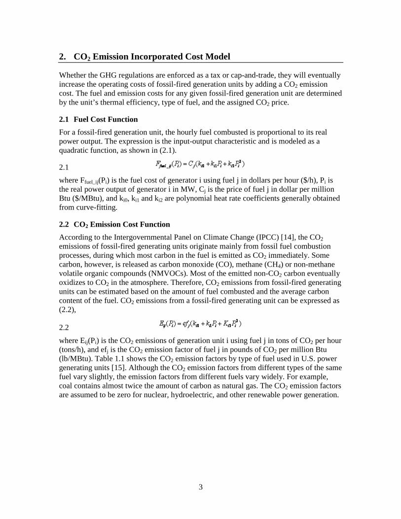
For a fossil-fired generation unit, the hourly fuel combusted is proportional to its real power output. The expression is the input-output characteristic and is modeled as a quadratic function, as shown in (2.1).

2.1

where Ffuel_ij(Pi) is the fuel cost of generator i using fuel j in dollars per hour ($/h), Pi is the real power output of generator i in MW, Cj is the price of fuel j in dollar per million Btu ($/MBtu), and ki0, ki1 and ki2 are polynomial heat rate coefficients generally obtained from curve-fitting.

2.2 CO2 Emission Cost Function

According to the Intergovernmental Panel on Climate Change (IPCC) [14], the CO2 emissions of fossil-fired generating units originate mainly from fossil fuel combustion processes, during which most carbon in the fuel is emitted as CO2 immediately. Some carbon, however, is released as carbon monoxide (CO), methane (CH4) or non-methane volatile organic compounds (NMVOCs). Most of the emitted non-CO2 carbon eventually oxidizes to CO2 in the atmosphere. Therefore, CO2 emissions from fossil-fired generating units can be estimated based on the amount of fuel combusted and the average carbon content of the fuel. CO2 emissions from a fossil-fired generating unit can be expressed as (2.2),

2.2

where Eij(Pi) is the CO2 emissions of generation unit i using fuel j in tons of CO2 per hour (tons/h), and efj is the CO2 emission factor of fuel j in pounds of CO2 per million Btu (lb/MBtu). Table 1.1 shows the CO2 emission factors by type of fuel used in U.S. power generating units [15]. Although the CO2 emission factors from different types of the same fuel vary slightly, the emission factors from different fuels vary widely. For example, coal contains almost twice the amount of carbon as natural gas. The CO2 emission factors are assumed to be zero for nuclear, hydroelectric, and other renewable power generation.

4

Table 2.1 CO2 Emission Factors (effuel) by Fuel Types [15]

Fuel Type CO2 Emission Factor

(lbs CO2/MBtu)

Coal

Bituminous 205

Subbituminous 213

Lignite 215

Anthracite 227

Oil

Distillate Oil 161

Jet Fuel 156

Kerosene 159

Petroleum Coke 225

Residual Oil 174

Gas

Natural Gas 117

Propane 139

The CO2 emission cost function of a fossil-fired generation unit can be expressed as the product of a given CO2 price and the total amount of CO2 emitted, as follows:

2.3

2.4

where FCO2_ij(Pi) is the CO2 emission cost of generator i using fuel j in $/h, and CCO2 is the given CO2 price in dollars per ton ($/ton), which is determined by regulations and markets.

5

2.3 Fuel-and-emission Cost Function

The fuel-and-emission cost function of a fossil-fired generation unit is the sum of the fuel cost function and the CO2 emission cost function, as follows:

2.5

2.6

where Ftotal_ij(Pi) is the fuel-and-emission cost function of generator i using fuel j in $/h.

6

3. Implication of CO2 emission costs on Generation Dispatch

In current market modes such as central day-ahead or real time energy markets, the introduction of CO2 emission costs, as shown in (5) and (6), changes fossil-fired generation costs and therefore the generation dispatch order. Fig. 3.1 shows the cost curves (fuel cost curve, CO2 emission cost curve and combined fuel-and-emission cost curve) of a typical 400 MW coal-fired generation unit (left plot) and 400 MW gas-fired generation unit (right plot) in relation to power output (MW), where the CO2 price is assumed to be 30 $/ton. Typical heat rate data of 400 MW fossil-fired generation units [16] are used to curve-fit the polynomial heat rate coefficients, as shown in Table 3.1. The fuel prices as of May 2008 (1.90 $/MBtu for coal and 10.35 $/MBtu for gas) are used. It is evident from Fig. 3.1 that, with a CO2 price of 30 $/ton, the CO2 emission costs of coal-fired generation unit are higher than that of gas-fired generation unit because coal has a higher CO2 emission factor than that of gas (215 lb/MBtu for coal and 118 lb/MBtu for gas in this case). However, the gas-fired generation unit has much higher fuel costs than that of coal-fired generation unit because of the higher gas price. The result is that the fuel-and-emission costs of gas-fired generation unit are much higher than that of coal-fired generation unit. Meanwhile, if the given CO2 price is high enough, the fuel-and-emission costs of the coal-fired generation unit might be higher than that of gas-fired generation unit. This CO2 price is called the breakeven price of CO2.

100 200 300 4000

0.5

1

1.5

2

2.5

3

3.5

4

4.5

5x 10

4

Output, P (MW)

Cos

ts ($

/h)

100 200 300 4000

0.5

1

1.5

2

2.5

3

3.5

4

4.5

5x 10

4

Output, P (MW)

Cos

ts ($

/h)

Figure 3.1 Cost curves of two 400 MW fossil-fired generation units

7

Table 3.1 Typical Fossil-fired Generation Unit Heat rate Data [16]

400 MW Steam-coal 400 MW Steam-gas 25% output (Btu/kWh)

10674 11267

40% output (Btu/kWh)

9783 10327


9252 9766


9045 9548


9000 9500

As shown in (6), for a given fossil-fired generation unit, the fuel-and-emission costs are sensitive to fuel price and CO2 price. Natural gas prices have been extremely volatile over the past few years, compared with relatively stable coal prices. Fig. 3.2 shows the average U.S. monthly power generation fuel price from Jan. 2005 to Dec. 2008 [17].

Figure 3.2 Power Generation Fuel Prices [17]

A sensitivity analysis of different gas prices for the breakeven price of CO2 using the maximum (12.74 $/MBtu), minimum (5.51 $/MBtu), and median (9.11 $/MBtu) gas prices over Jan. 2005 to Dec. 2009 period was performed. A constant coal price of 1.9 $/MBtu was used in the analysis. Fig. 3.3, Fig. 3.4 and Fig. 3.5 show the results. In each

8

figure, the two horizontal axes are the power output of the two units from 100 MW (minimum) to 400 MW (maximum) and the CO2 price from 0 $/ton (minimum) to 350 $/ton (maximum) respectively. The vertical axis is the units’ fuel-and-emission costs in $/h.

Figure 3.3 Sensitivity analysis of gas prices at 5.51 $/MBtu


9


Fig. 3.3, Fig. 3.4 and Fig. 3.5 clearly show how a variation in gas price will alter the breakeven price of CO2 and therefore affect the dispatch order among fossil-fired generation units (variable operating and maintenance costs are ignored).

� As shown in Fig. 3.3, when the gas price is 5.51 $/MBtu and coal price is 1.9 $/MBtu, the breakeven price of CO2 is 98 $/ton. At CO2 prices lower than this, the coal-fired generation unit is more competitive. At CO2 prices higher than this, the gas-fired generation unit is more competitive.

� As shown in Fig. 3.4, when the gas price is 9.11 $/MBtu and coal price is 1.9 $/MBtu, the breakeven price of CO2 is 190 $/ton. At CO2 prices lower than this, coal-fired generation is more competitive. At CO2 prices higher than 190 $/ton, gas-fired generation is more competitive.

� As shown in Fig. 3.5, when the gas price is 12.94 $/MBtu and coal price is 1.9 $/MBtu, the breakeven price of CO2 is 285 $/ton. At CO2 prices lower than 285 $/ton, coal-fired generation is more competitive. At higher CO2 prices, the gas-fired generation unit is more competitive.

10

4. CO2 Emission-incorporated AC Optimal Power Flow

The cost model developed in section III can be built into optimal power flow (OPF) methodology. The purpose of CO2 emission-incorporated ac OPF is to minimize a combined objective function of fuel costs and CO2 emission costs by changing various system control variables, subject to both equality and inequality constraints.

4.1 Objective function

The objective function of the traditional OPF can take different forms, such as minimizing generation costs, electrical losses, or control changes. The objective function of the CO2 emission-incorporated ac OPF is to minimize both fuel costs and CO2 emission costs, as shown in (4.1).

4.1

where the Ftotal_ij(Pi) is the fuel-and-emission cost function expressed as (3.5) and (3.6), Ng is the number of generators in the system.

4.2 Equality and Inequality constraints

These equality and inequality constraints represent power balance constraints and various operating limits within the system. The equality constraints are system real and reactive power balance, as shown in (4.2) and (4.3),

4.2

4.3

where Pi is the real power output from generator i, PLoad is the system total real power load, PLoss is the system total real power loss, Qi is the reactive power output from generator i, QLoad is the system total reactive power load, and QLoss is the system total reactive power loss. The inequality constraints are generator real and reactive power limits, bus voltage and angle limits, and transmission branch loading limits, as shown in (4.4), (4.5), (4.6), (4.7), and (4.8), respectively,

4.4

4.5

4.6

4.7

4.8

11

where Ek is the magnitude of voltage at bus k, δk is the voltage phase angle at bus k, and MVA mn is the power flow of the transmission branch between bus m and n.

There are several mathematical programming approaches available to solve the OPF problem. Among these approaches linear programming (LP) is fully developed and in common use. The CO2 emission-incorporated ac OPF can be solved using the LP method by iterating between solving the power flow equations and then solving a LP to change the system control variables to remove any constraint violations. The proposed CO2 emission-incorporated ac OPF can be realized in commercial or research software, or as stand-alone software. This paper uses commercial software, with CO2 cost model developed in Section III, to implement the CO2 emission-incorporated ac OPF.

12

5. Numerical Studies

5.1 Test System and Simulation Cases

The 24-bus IEEE Reliability Test System (RTS) [18], with modifications, is used to demonstrate and assess the proposed CO2 emission-incorporated ac OPF and its primary impacts on power system dispatch and operations. The IEEE RTS system represents the characteristics of a large power system. The topology is shown in Fig. 5.1 [19]. The IEEE RTS has 24 buses, 38 transmission lines and transformers and a total load of 2850 MW. The transmission lines are at two voltage levels: 138 kV and 230 kV. The generation capacity consists of 300 MW of hydro, 800 MW of nuclear, 1274 MW of steam fossil coal, 951 MW of steam fossil oil, and 80 MW of combustion turbines with total generating system capacity equal to 3405 MW. In order to include the common steam fossil natural gas generation, the simulations presented in this paper replace the 951 MW of fossil steam oil with 951 MW of fossil steam gas.

Figure 5.1 IEEE Reliability Test System [19]

13

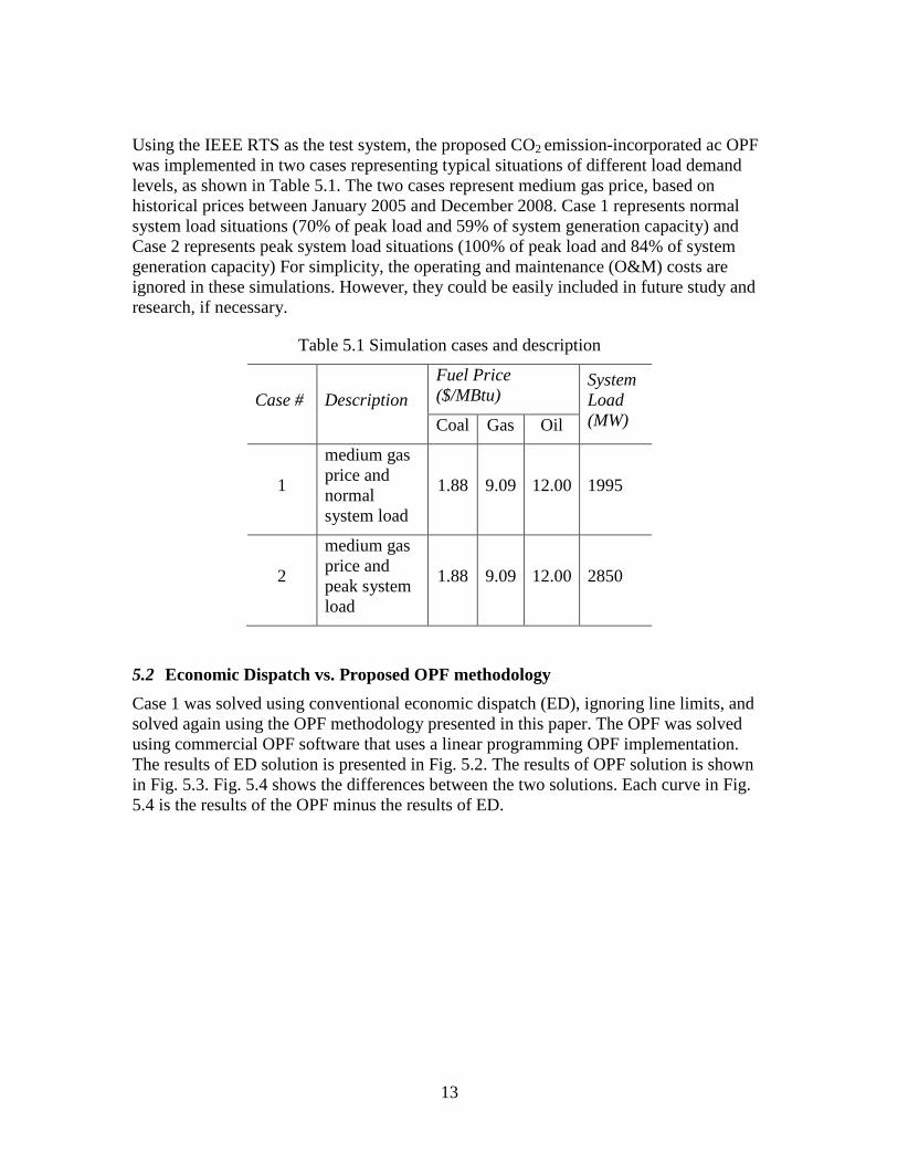
Using the IEEE RTS as the test system, the proposed CO2 emission-incorporated ac OPF was implemented in two cases representing typical situations of different load demand levels, as shown in Table 5.1. The two cases represent medium gas price, based on historical prices between January 2005 and December 2008. Case 1 represents normal system load situations (70% of peak load and 59% of system generation capacity) and Case 2 represents peak system load situations (100% of peak load and 84% of system generation capacity) For simplicity, the operating and maintenance (O&M) costs are ignored in these simulations. However, they could be easily included in future study and research, if necessary.

Table 5.1 Simulation cases and description

Case # Description

Fuel Price ($/MBtu)

System Load (MW) Coal Gas Oil

1

medium gas price and normal system load

1.88 9.09 12.00 1995

2

medium gas price and peak system load

1.88 9.09 12.00 2850

5.2 Economic Dispatch vs. Proposed OPF methodology

Case 1 was solved using conventional economic dispatch (ED), ignoring line limits, and solved again using the OPF methodology presented in this paper. The OPF was solved using commercial OPF software that uses a linear programming OPF implementation. The results of ED solution is presented in Fig. 5.2. The results of OPF solution is shown in Fig. 5.3. Fig. 5.4 shows the differences between the two solutions. Each curve in Fig. 5.4 is the results of the OPF minus the results of ED.

14

Figure 5.2 CO2 emissions and costs in case 1 (ED)

Figure 5.3 CO2 emissions and costs in case 1 (OPF)

The ED results show that the CO2 prices have no effect until $130/ton. From this, it would be expected that the same price would affect dispatch between coal and gas units in the OPF results. However, the OPF results show the redispatch from coal to gas starts at $70/ton. This was because of the line congestion in the system regardless of CO2 price. From $0/ton to $70/ton, redispatch to relieve congestion was among coal units; some were reduced in output, some were increased, while keeping the fuel use (and thus CO2

15

output) and fuel costs constant. Because the fuel use (and costs) was constant, and there were no dispatch changes in the ED solution, the difference in fuel cost and CO2 emissions were constant. The growing positive difference in emissions cost and total cost between the ED and OPF solutions is because of increased CO2 price.

Figure 5.4 Differences of CO2 emissions and costs between ED and OPF in Case 1.

At $70/ton, in the OPF solution, it became more economical to redispatch to gas units to relieve congestion. This didn't happen until $130/ton in the ED solution. This difference can only be explained by the fact that the constraints on line flows have changed the nonlinear system to a system where the change to gas happens at a lower CO2 price.

This is confirmed by Fig. 5.5, which shows total dispatch by fuel type for varying CO2 price. Between $0 and $50 (actually $70, but this graph changes in increments of $50) total coal dispatch in the OPF stays the same, but individual coal units are still changing. So up until $70 (Fig. 5.5) emissions and fuel costs in the OPF are constant, so the difference in these values between OPF and ED stay about constant. Total costs rise in the OPF because payments for CO2 increase, so the difference in total costs increases. Beyond $70, redispatch to gas begins in the OPF, but not in the ED, so difference in fuel costs increase, and difference in CO2 decreases. Fig. 5.6 shows the loading of some selected units in the OPF and ED cases, which confirms that loading was changing on individual units below the $70/ton CO2 price.

This continues until the CO2 price hits $130, which is where redispatch to gas begins in the ED case, so the ED costs begin to rise and the ED CO2 emission begins to fall, and the differences between the two in Fig.5.5 decrease.

16

Beyond that, the comparison becomes a complicated function of system topology, congestion, CO2 price, and other factors, and the results are shown on the Fig. 5.5.

Note that the total power generated in the OPF case is lower than in the ED case, and this is because losses are lower. But the cost of operating (fuel cost) is still higher in the OPF case.

Figure 5.5 Generation dispatch comparison between ED and OPF

Figure 5.6 Selected units loading in case 1(ED and OPF)

17

6. Simulations: Economic Dispatch vs. Optimal Power Flow

6.1 Simulation Results of Case 1 and Case 2

Fig. 6.1 shows the changes in power output from the five generation types in relation to varying CO2 prices for the OPF case 1. The changes in system total CO2 emissions and costs (CO2 emission costs, fuel costs and fuel-and-emission costs) in relation to varying CO2 prices are already shown in Fig. 6.1. The CO2 prices are increased from 0 $/ton to 450 $/ton in steps of 10 $/ton.

As illustrated in Fig. 6.1, without CO2 emissions constraints (CO2 price is 0 $/ton), the system load can be met most economically by hydro, nuclear, and coal-fired generation. The gas-fired and oil-fired generation is not dispatched. As the CO2 price increases, generation output starts to shift from coal-fired to gas-fired units at a CO2 price of 70 $/ton. At a CO2 price of 180 $/ton, the gas-fired generation output exceeds the coal-fired generation output. The shifting between coal-fired and gas-fired generation continues until the CO2 price reaches 280 $/ton. At this point, most of the available 951 MW gas-fired generation is operating (873 MW). Although there is still some gas-fired generation capacity left (78 MW), the shifting between coal-fired generation and gas-fired generation continues at a very small rate due to system congestion, regardless of how high the CO2 price rises.

Meanwhile, total system CO2 emissions have changed due to shifting from coal-fired to gas-fired generation, at the expense of increasing operating costs. As shown in Fig. 6.1, the total system CO2 emissions decrease from 928 tons/h at a CO2 price of 0 $/ton to 514 tons/h at a CO2 price of 280 $/ton. The CO2 emissions decrease 44.6%. Although the system fuel-and-emission costs increase from 18,595 $/h at a CO2 price of 0 $/ton to 223,159 $/h at a CO2 price of 280 $/ton, the system fuel costs increase from 18,595 $/h to 79,255 $/h and stay almost constant afterward. The system fuel costs increase 326%.

Fig. 6.2 shows the changes in power output from the five generation types in relation to varying CO2 prices for the OPF case 2. The changes in system total CO2 emissions and costs (CO2 emission costs, fuel costs and fuel-and-emission costs) in relation to varying CO2 prices are shown in Fig. 6.3.

As illustrated in Fig. 6.2, without the CO2 emission constraint (CO2 price is 0 $/ton), the peak system load can be met by hydro, nuclear, coal-fired, and gas-fired generation. The oil-fired generation is not dispatched. With increasing CO2 price, the generation output starts to shift from coal-fired generation units to gas-fired generation units at a CO2 price of 80 $/ton. At a CO2 price of 180 $/ton, the gas-fired generation output almost equals the coal-fired generation output. At this point, most of the available 951 MW of gas-fired generation is operating (908 MW). Although there is still some gas-fired generation capacity left (43 MW), the shifting between coal-fired and gas-fired generation continues at a very low rate due to system congestion, regardless of how high the CO2 price rises.

18

Figure 6.1 Changes in power output in case 1

Meanwhile, the total system CO2 emissions have changed because of the shift from coal-fired to gas-fired generation. As shown in Fig. 6.3, the total system CO2 emissions decrease from 1,453 tons/h at a CO2 price of 0 $/ton to 1,327 tons/h at a CO2 price of 180 $/ton. The CO2 emissions decrease 8.7%. Although the system fuel-and-emission costs increase from 79,276 $/h at a CO2 price of 0 $/ton to 335,155 $/h at a CO2 price of 180 $/ton, the system fuel costs only increase from 79,276 $/h to 96,329 $/h and stay almost constant afterward. The system fuel costs increase 21.5%.

19

Figure 6.2 Power output in case 2 (OPF)

Figure 6.3 CO2 emissions and costs in case 2 (OPF)

20

7. Discussion of ED vs. OPF Results

Comparisons of optimal dispatch for this test system, which has significant transmission congestion even at moderate load levels, show significant differences between conventional dispatch calculations, in which congestion is not considered, and OPF calculations, in which it is. This indicates that line congestion will have a significant effect on reductions in CO2 emissions and must be considered. Therefore OPF must be used in any simulations of redispatch to reduce CO2 emissions. Some redispatch for congestion relief, especially at low CO2 prices, will be among units of the same fuel, resulting in little effect on system costs and CO2 emissions. As CO2 prices increase, however, redispatch to relieve congestion will be from coal to natural gas, resulting in lower costs but higher emissions.

Simulation results are sensitive to system load level. In the normal system load situation (case 1), the load can be met by nuclear, hydro and coal-fired generation; the gas-fired generation units are not needed. When a certain amount of CO2 cost is added, the power from coal-fired units starts to shift to gas-fired generation units. At a high enough CO2 price, most of the coal-fired generation shifts to gas-fired. However, in the peak system load situation (case 2), a large amount of gas-fired generation was already dispatched to meet the load even without CO2 emission constraints. When a CO2 cost is added, the system does not have enough gas-fired generation capacity left to replace the large amount of coal-fired generation. For example, only 283 MW of coal-fired generation was replaced by gas-fired generation in case 2, compared with 911 MW in case 1. The result is that the CO2 emissions were reduced by 8.7% only in case 2, but were reduced by 44.6% in case 1. Higher load levels results in less CO2 reduction because of limited gas-fired capacity.

The results are based on the IEEE RTS, modified for this project, which has specific generation mix and transmission constraints. The results will be different in other systems with different generation mix and transmission constraints. The resulting CO2 emission reduction is restricted to gas-fired generation capacity in the existing generation mix that is available to be dispatched in place of coal-fired generation, as well as the transmission constraints that determine the possibility of such generation redispatch.

21

8. Time Series Simulations

Performing OPF gives one “snapshot” of the power system conditions at an instant in time. To better represent variable characteristics of renewable generation, the charge and discharge of energy storage, and the CO2 emissions from a system over a period, a series of OPF simulations are run with time-varying inputs. Simulated output of renewable generators are specified based on historical or simulated profiles of renewable resources. Hydroelectric generation and energy storage are scheduled outside the OPF and input as time series data. Electrical load demand also varies with time depending on time of day, season, and year. Load data are also represented as a set of points in time. This dissertation utilizes a time series of renewable generation output, hydroelectric and energy storage, and system load as input data to the OPF. Finally, a set of solutions for the specified time period will be obtained.

8.1 Renewable Energy Simulation Cases

Various study cases are designed based on different renewable generation profiles, system load profiles, CO2 prices, solution types, and length of time simulated. The average fuel prices in the year 2008 [20] are used as the fuel costs for each generator in the IEEE RTS system (2.06 $/MBtu for coal, 9.34 $/MBtu for gas, and 16.56 $/MBtu for oil, according to average fuel prices from January 2008 to November 2008). Fuel cost for nuclear is 0.44$/MBtu, as per the average U.S. nuclear fuel price in 2006 [21]. The CO2 emission factors are 215 lb/MBtu, 117 lb/MBtu, and 161 lb/MBtu for coal, gas, and oil, respectively [22]. Assumed CO2 prices of zero and 50 $/ton are studied in the proposed cases. Capacity credits are calculated when wind or solar are integrated into the test system. In this research, capacity credit is assumed to be 25.2 percent for wind and 89.5 percent for solar, based on the calculated capacity credits in [23].

Renewable generators are added into the IEEE RTS in cases 1-9 to study their effect on GHG emissions. Three renewable generators, 100 MW capacity each, are connected to bus no. 8 of the IEEE RTS system through a new transmission line. The IEEE RTS with renewable generation is shown in Figure 8.1.

22

Figure 8.1 Modified IEEE reliability test system with renewable generation, adapted from [24]

In order to calculate the system operating cost with renewable generation, a system forecasting fee is assumed to be 0.10 $/MWh, based on [25]. This research also applies 0.010 $/MWh of net deviation charge for electricity produced from renewable generation.

An energy storage system rated 10MW is added into the IEEE RTS in case 11 and located at the same bus as renewable generation. An annualized fixed operation and maintenance cost for the storage unit is assumed to be 15 $/kWh [26]. The storage is assumed to charge and discharge one time in each 24-hour period. The number of operating days for this storage is approximately 250 days per year.

The methodology solves the OPF solution for cases 1-9 and 11 to determine the MW dispatched output, locational marginal prices for each node, and total operating cost. Meanwhile, the security constrained optimal power flow (SCOPF) is run for case 10 to

23

address security issue by considering contingencies. In this case, three contingencies are specified and included in the analysis. Each contingency is the loss of a transmission line in the power system. The three contingencies include loss of a transmission line from bus 15 to bus 24, a transmission line from bus 13 to bus 23, and a transmission line from bus 14 to bus 11.

The time series of renewable generation and system load are applied in each case. The simulation runs 24 time steps (hours) for daily load and generation profiles, and 8,784 time steps (hours) for year-round profiles. Table 8.1 summarizes the simulation cases and their detailed descriptions, including generation and load profiles, solution type, and CO2 prices.

Table 8.1 Simulation Cases and Description

Case No.

Renewable Generation Load Profile

CO2 Price

($/ton)

Solution Type

Number of Time

Point (hour)

Type Profile

1 Wind Low varying Typical summer day 0 OPF 24

2 Wind Medium varying Typical summer day 0 OPF 24

3 Wind High varying Typical summer day 0 OPF 24

4 Wind Low varying Typical summer day 50 OPF 24

5 Wind Medium varying Typical summer day 50 OPF 24

6 Wind High varying Typical summer day 50 OPF 24

7 Solar Summer day Typical summer day 0 OPF 24

8 Solar Summer day Typical summer day 50 OPF 24

9 Wind Year 2004 Scaled year 2004 50 OPF 8784

10 Wind Year 2004 Scaled year 2004 50 SCOPF 8784

11 Wind/

Storage Medium varying Typical summer day 0 OPF 24

24

The three different daily wind profiles listed in Table 5.1 are based on generation output data [27] from ERCOT’s wind generation resources and are used as the MW output of the new added wind power plants. The three daily wind patterns include low varying generation output, medium varying output, and high varying output.

The load profile that is used is a typical summer day load based on the ERCOT historical load data [28] for a summer day in 2008 and scaled down to the system load of the IEEE-RTS. Figure 5.22 shows plots of the typical summer day load profile versus the three wind-generation output profiles.

Figure 8.2 Typical summer day load profile and three wind generation output profiles.

Solar generation is added to the IEEE RTS in cases 7 and 8. The output of a solar power plant is much more predictable than that of a wind generator, because meteorological models predict clouds and sunlight much more accurately than wind. The solar power plant always generates output between sunrise and sunset unless there is a significant amount of clouds or other extreme weather conditions. In this research, a solar generation output profile is developed and scaled, based on the output profile of a solar array in the ERCOT control area on a summer day, as described by [29]. Figure 8.3 presents the typical summer day load profile versus the solar profile.

25

Figure 8.3 Typical summer day load profile and a solar generation output profile

Besides single-day simulations, simulations are also performed for a one-year span. In these annual simulations, the OPF and SCOPF are run for 8,784 time points, which represent the 8,784 hours of the year 2004. ERCOT’s 2004 historical load data [28] is scaled down and applied as a year-round load pattern, including MW and MVar load for each load bus of the IEEE RTS. Figure 5.24 presents the annual scaled MW load profile that is used in this dissertation. Wind generation hourly output data recorded in the year 2004 [27] is applied as the MW output of added wind generation resources.

26

9. Renewable Simulation Results

9.1 Results for Base System

Generation dispatch for the modified IEEE RTS with no renewable generation and no CO2 price is presented in Figure 9.1. Nuclear power plants are dispatched as base load units, which always run at the rate of their maximum output. Thus the output of nuclear plants are seen as constantly flat during the day. Hydro plants, however, are committed usually only on peak-load hours of the day due to the limitation of the amount of water available to generate. In this model, the hydro units start to operate at 3 PM and continue running until 8 PM. Coal-fired power plants follow daily load demand by raising their output during on-peak hours and reducing their output during off-peak hours. The coal-fired power plants, however, slightly drop their output due to congestion caused by the hydro plants. The combustion turbine plants are not dispatched due to the high fuel price of petroleum oil.

Figure 9.2 shows the marginal price at the bus where renewable generation will be installed in later simulations. As seen from this plot, the congestion occurred during the peak period from 3 PM to 8 PM. Congestion costs in the locational marginal price are about zero for most of the day until hydro plants start to operate. Congestion costs increased to about $50 per MWh when hydro units are committed. In this lossless model, the locational marginal price consists of marginal congestion price and marginal energy price. Locational marginal prices are about $18.93 to $24.91 per MWh during the off-peak period and increase to $110.43 per MWh during the on peak period because of congestion caused by the hydro units.

Figure 9.1 Generation dispatch without renewable generation installed

27

Figure 9.2 Marginal price at renewable generation bus before renewables are installed

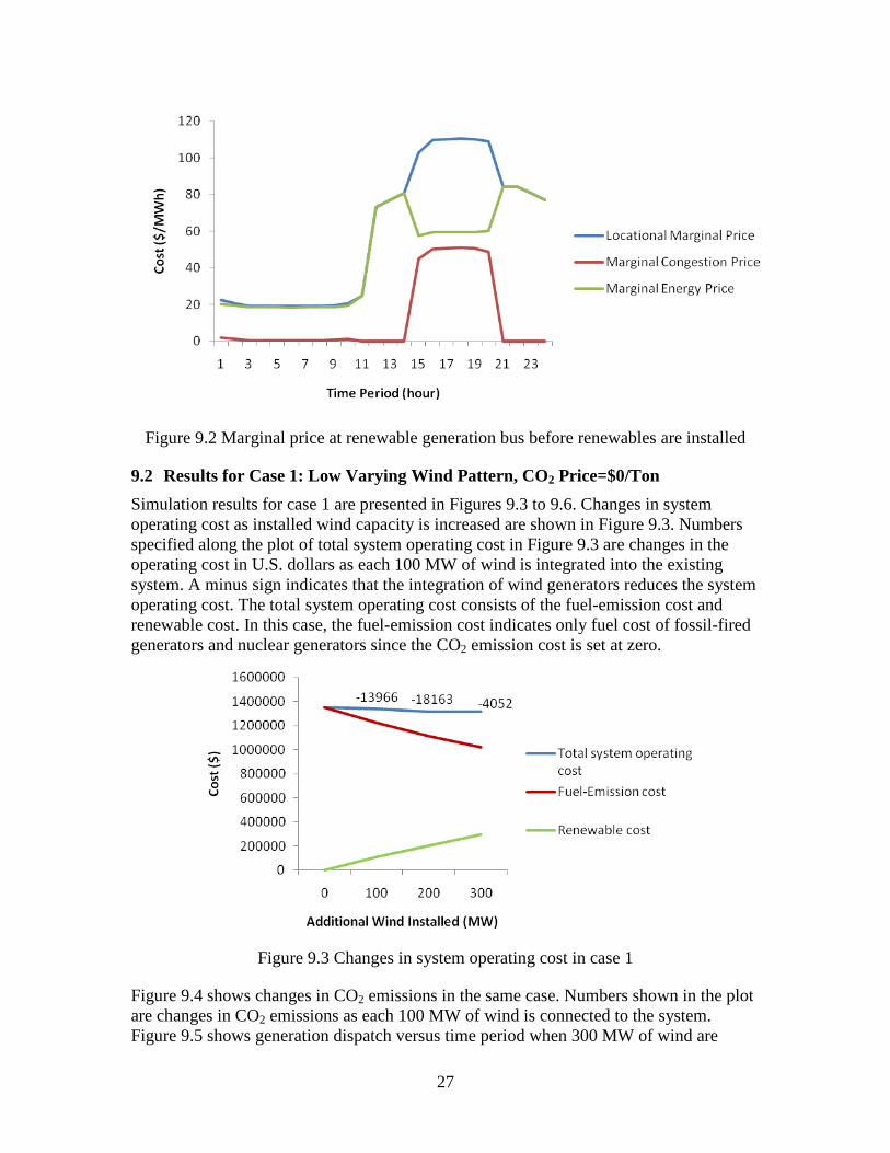
9.2 Results for Case 1: Low Varying Wind Pattern, CO2 Price=$0/Ton

Simulation results for case 1 are presented in Figures 9.3 to 9.6. Changes in system operating cost as installed wind capacity is increased are shown in Figure 9.3. Numbers specified along the plot of total system operating cost in Figure 9.3 are changes in the operating cost in U.S. dollars as each 100 MW of wind is integrated into the existing system. A minus sign indicates that the integration of wind generators reduces the system operating cost. The total system operating cost consists of the fuel-emission cost and renewable cost. In this case, the fuel-emission cost indicates only fuel cost of fossil-fired generators and nuclear generators since the CO2 emission cost is set at zero.

Figure 9.3 Changes in system operating cost in case 1

Figure 9.4 shows changes in CO2 emissions in the same case. Numbers shown in the plot are changes in CO2 emissions as each 100 MW of wind is connected to the system. Figure 9.5 shows generation dispatch versus time period when 300 MW of wind are

28

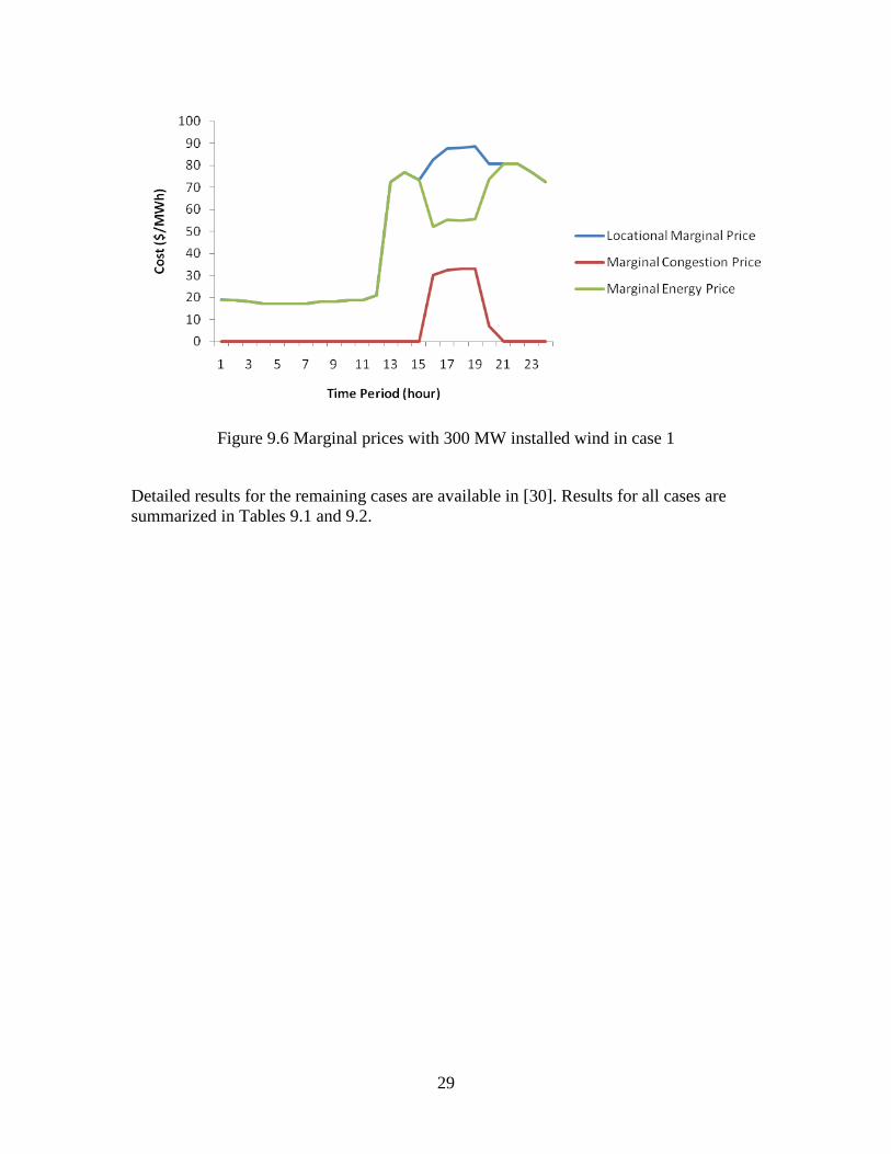
installed in the system. Figure 9.6 presents marginal price with 300 MW installed wind in case 1. This figure includes plots of locational marginal price, marginal energy price, and marginal congestion price. The marginal loss price is zero as this system is assumed to be a lossless system.

Figure 9.4 Changes in CO2 emissions in case 1

Figure 9.5 Generation dispatch with 300 MW installed wind in case 1

29

Figure 9.6 Marginal prices with 300 MW installed wind in case 1

Detailed results for the remaining cases are available in [30]. Results for all cases are summarized in Tables 9.1 and 9.2.

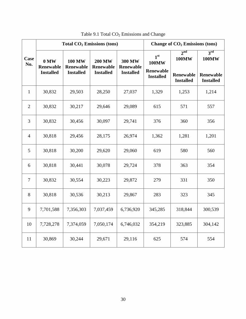
30

Table 9.1 Total CO2 Emissions and Change

Case No.

Total CO2 Emissions (tons) Change of CO2 Emissions (tons)

0 MW Renewable Installed




1st 100MW

Renewable Installed

2nd 100MW

Renewable Installed

3rd

100MW

Renewable Installed

1 30,832 29,503 28,250 27,037 1,329 1,253 1,214

2 30,832 30,217 29,646 29,089 615 571 557

3 30,832 30,456 30,097 29,741 376 360 356

4 30,818 29,456 28,175 26,974 1,362 1,281 1,201

5 30,818 30,200 29,620 29,060 619 580 560

6 30,818 30,441 30,078 29,724 378 363 354

7 30,832 30,554 30,223 29,872 279 331 350

8 30,818 30,536 30,213 29,867 283 323 345

9 7,701,588 7,356,303 7,037,459 6,736,920 345,285 318,844 300,539

10 7,728,278 7,374,059 7,050,174 6,746,032 354,219 323,885 304,142

11 30,869 30,244 29,671 29,116 625 574 554

31

Table 9.2 System Operating Cost and Change

Case No.

System Operating Cost ($) Change of System Operating Cost

($)





1st

100MW

Renewable Installed

2nd 100MW

Renewable Installed

3rd

100MW

Renewable Installed

1 1,351,283 1,337,318 1,319,155 1,315,103 13,966 18,163 4,052

2 1,351,283 1,340,967 1,332,659 1,316,205 10,316 8,309 16,453

3 1,351,283 1,342,395 1,333,257 1,328,747 8,889 9,137 4,511

4 2,872,811 2,852,572 2,835,404 2,829,446 20,239 17,168 5,958

5 2,872,811 2,858,361 2,847,077 2,839,298 14,450 11,284 7,779

6 2,872,811 2,860,381 2,848,784 2,841,974 12,430 11,597 6,810

7 1,351,283 1,330,587 1,312,033 1,309,308 20,696 18,555 2,724

8 2,872,811 2,846,217 2,821,432 2,805,262 26,594 24,785 16,170

9 649556225 643887780 639363928 636796507 5,668,446 4,523,851 2,567,422

10 662455004 656954096 651740065 648247222 5,500,908 5,214,031 3,492,843

11 1,347,216 1,336,524 1,328,462 1,312,356 10,692 8,062 16,105

32

10. Interpretation of Renewable Results

Results of the simulations demonstrate how integration of low carbon emission generation affects the test system. Effects include system dispatch, emissions, cost, and reliability. Effects of energy storage are also discussed in this section.

10.1 System Dispatch

When renewable generators are integrated into the system, they generate inconstant output based on available fuels from nature such as wind and sunlight. These low carbon generation outputs can change at any time. Their output is considered a must-take resource and are unavailable for the automatic generator control (AGC) to adjust.

Output from nuclear power plants is almost always constant, and nuclear plants have relatively low operating costs. Nuclear units are assigned to run at full capacity all the time, with an occasional exception of coast down at the end of a fuel cycle. As a result, the generation dispatch of nuclear power plants is constantly flat throughout the day.

Hydro power plants are normally scheduled outside the system dispatch. Unlike nuclear power plants, hydro plants cannot run all day long due to limitations in the amount of water, depending on seasonal climate and geography. Hydro plants in the system simulated for this dissertation operate only during on-peak load, which is from 3:00 PM to 8:00 PM.

Due to their high fuel price, combustion plants burning petroleum oil are never dispatched in this model. The outputs of these generators are zero all the time. For some control areas, generators with oil as fuel will be dispatched only when gas-fired generators are not available.

As renewable generators (wind generators or solar plants) are integrated into the IEEE RTS, the system dispatch of coal-fired power plants and gas-fired power plants is reduced. Coal-fired power plants usually run as base load units but follow changing load as needed. In the simulation results, coal-fired generators drop their output during off-peak load when all gas-fired generation has been reduced to low or zero output. The coal units then raise their output to follow load as it increases. In Figure 5.7, when no wind generation is installed, coal-fired plants drop their total output slightly below 800 MW at 6:00 AM. With integration of wind, coal-fired power plants lower their output even more during off-peak load because of the additional energy contributed to the system by the wind generators. According to Figure 5.54, dispatched generation of coal plants drop to 677 MW, 603 MW, and 503 MW at off-peak load with integration of wind at 100 MW, 200 MW, and 300 MW, respectively. Although it is unusual to reduce the output of a coal-fired generator below 50 percent of its rated capacity, some power plants can go below 50 percent using special operating procedures and plant designs.

As load increases during the day, coal-fired power plants increase their output to meet the demand. These units, however, slightly drop their outputs during the on-peak period due to congestion caused by hydro plants. The MW output of coal-fired generation units at peak load are flattened due to the integration of low varying wind output in case 1 and case 4. In these cases, wind generation relieves some of the congestion caused by hydro

33

units. Wind generation is low during the congestion period in the medium-varying and high-varying wind profiles, however, much less congestion relief is provided, and coal output is still reduced during peak load in these cases. The generation dispatch of coal responds differently with each generation output profile of renewable generation. Figure 10.1 presents the generation dispatch of coal-fired generation units with different wind capacity installed for case 1. Plots for other cases are shown in [30].

Figure 10.1 Generation dispatch for coal-fired power plants in case 1

Gas-fired generating units in this simulation are used to support other generators to meet load demand. Based on their fuel price, which is higher than coal or nuclear units, they are dispatched at peak demand of the day, after all lower-cost gas and coal units are already operating at full capacity. With the integration of renewable generators, gas-fired generating units lower their output during the peak period. Figure 10.2 shows generation dispatch for gas-fired power plants in case 1. Each additional unit of renewable generation further reduces the output of the gas fired plants. Similar to the economic dispatch of coal-fired power plants, system dispatch responds differently with each output profile of renewable generation. Generation dispatch of gas fired generation units for other cases are shown in [30].

34

Figure 10.2 Generation dispatch for gas-fired power plants in case 1

10.2 Emissions

Based on the previous plots of changes in CO2 emissions, an integration of low carbon emission generators certainly reduces CO2 emissions. The reduction of CO2 emissions, however, is not proportional to each MW capacity of renewable generators installed. As shown in the simulation results, the change in CO2 emissions for each step of 100 MW installed wind or solar is not linear. This phenomenon is explained by several factors that affect system dispatch. These factors include fossil-fired generating plant design, the need for more operating gas-fired reserve units as renewable penetrations increase, and changes in transmission congestion.

According to the results, the reduction in CO2 emissions decreases for every 100 MW increase in wind generation. In case 1, reductions of CO2 emissions are 1,329 tons, 1,253 tons, and 1,214 tons for 100 MW, 200 MW, and 300 MW wind installed, respectively. For each increasing one hundred megawatts of wind, case 2 shows 615 tons, 571 tons, and 557 tons of CO2 emission reduction while case 3 shows 376 tons, 360 tons, and 356 tons, respectively. For the system costing $50/ton CO2, case 4 shows 1,362 tons, 1,281 tons, and 1,201 tons of CO2 reduction, while CO2 emission reductions in case 5 are 619 tons, 580 tons, and 560 tons when the system is integrated with 100 MW, 200 MW, and 300 MW of wind, respectively. Case 6 shows reductions of 378 tons, 363 tons, and 354 tons. Running the simulation for a whole year confirms this trend. The CO2 emission reductions of case 9 are 345,285 tons, 318,844 tons, and 300,539 tons further reduction for each additional 100 MW wind installed. Case 10 shows 354,219 tons, 323,885 tons, and 304,142 tons, for 100 MW, 200 MW, and 300 MW wind installed, respectively. Variations among the cases are due to the varying amounts of energy produced by the different wind profiles.

35

Integration of solar power plants, however, produces a different trend of CO2 emission reduction. CO2 emission reductions for case 7 are 279 tons, 331 tons, and 350 tons, while case 8 shows a reduction of 283 tons, 323 tons, and 345 tons for 100 MW, 200 MW, and 300 MW of solar power plants, respectively. For this system, each 100 MW of solar produces more CO2 reductions than the previous 100 MW. This is because as more solar generation is added, natural gas generators can be turned off, because of the higher capacity credit of solar energy. The reductions obtained from solar differ from those of wind cases because the total energy produced is different in each case.

Figure 10.3 shows the total CO2 emissions of a zero CO2 price system with different installed renewable types and profiles. According to this plot, the existing power system with low varying wind emits the lowest CO2. When integrated with solar or the high varying wind profile, the test system emits higher CO2. Similar trends can be observed in the case with a $50/ton CO2 price, as shown in Figure 10.4. Little change is seen when a CO2 price of $50/ton is added because the solar and wind energy do not change, and $50/ton is not high enough for this system to significantly shift from coal- to gas-fired generation. Not shown in this simulation, however, is the incentive that the CO2 price presents to build new solar and wind generators. This is reflected in higher LMPs paid to renewable generators.

Figure 10.3 CO2 emissions in a zero CO2 price system

36

Figure 10.4 CO2 emissions in a $50/ton CO2 price system.

Case 11 analyzes how energy storage combined with renewables affects system operations and CO2 emissions. Storage rated 10 MW and 120 MWh is added to the medium-varying profile wind generation case, case 2. Figure 10.5 compares total CO2 emissions in case 11 and case 2. Both cases utilize the same conditions, but there is no energy storage applied to case 2. In case 11, storage charges from 9:00 PM to 9:00 AM and then discharges electricity back to the system from 9:00 AM to 9:00 PM. According to Figure 5.53, CO2 emissions in case 11 are slightly higher than the emissions in case 2.

In case 11, more MW capacity of coal-fired generating units, which have higher CO2 emissions factors, are dispatched to charge the battery energy storage unit at night. Energy storage then is reducing gas-fired generation during the day as it discharges electricity back to the grid. As a result, a net increase in CO2 emissions is observed. If it is desired to use storage to reduce CO2 emissions, its charge and discharge cycles will have to be optimized for that purpose. To obtain more accurate results, efficiency of the energy storage unit should be considered into the analysis.

37

Figure 10.5 Total CO2 emissions in case 2 and case 11

10.3 System Operating Cost

System operating cost in this research consists of two major components: fuel-emissions cost, which is the total cost of fuel and emissions charges, and renewable generation cost, which only includes payments to the renewable generator, not the capital cost of the generator. As the MW capacity of installed renewable generation increases, the fuel-emission cost decreases due to less MW capacity of the conventional generation dispatched. The renewable generation cost increases when renewable generators produce more electricity. Overall, the system operating cost decreases as the amount of renewable generators installed increases. Similar to CO2 emissions, the changes in system operating cost are not linear with installed capacity. The factors involved in this issue are the same factors that affect CO2 emissions.

The type of renewable resources and availability of wind or solar resources, which determines the generation output profiles, influences the system operating cost. Figure 10.6 illustrates the system operating with different renewable generators. The operating cost of the solar-integrated system is the lowest, because gas-fired generators were shut down because of solar’s high capacity factor. The system with a low-varying wind profile has a lower operating cost than the systems with medium-varying and high-varying wind profiles, because the low-varying profile results in the most energy produced by wind. The operating cost for the system with high varying wind profile is the highest, because it produced the least energy.

With the high capacity credit of solar, fewer gas-fired generators are committed as reserves, and as a result, lower overall operating costs are observed in case 7 and case 8. Operating costs with wind are affected by the amount of energy generated, when it is generated, and what types of generation it offsets. The low-varying wind profile in case 1 and case 4 has the highest energy production of the three wind cases, so it offsets a large amount of fossil-fired generation, giving the greatest reduction in CO2 emissions and

38

operating costs of the three cases. Considering the time when wind energy is generated, the low-varying wind profile also relieves congestion from 3:00 PM to 8:00 PM when hydro power generators operate, further reducing operating costs by reducing congestion costs. The medium-varying wind profile in case 2 and case 5, and the high-varying wind profile in case 3 and case 6, however, provide little congestion relief because there are very low wind outputs during the congestion period.

Higher system operating costs are seen in the system with a $50/ton CO2 price when compared to those of the system with $0/ton CO2 price, because that CO2 price must be paid on coal and gas generation, and because wind and solar are paid the higher LMP that results from the CO2 price. Figure 10.7 shows system operating cost for a $50/ton CO2 price system. Based on this figure, the system with solar has the lowest operating cost, while the systems with higher-varying profiles have higher system operating costs.

The operating cost of the system integrated with energy storage is analyzed in case 11. Figure 10.8 compares system operating costs in case 11 and case 2 to illustrate the difference in the system with and without energy storage. According to the results, the system operating cost in case 11 is lower than the operating cost in case 2. This is because the storage is charged at night from low-cost coal-fired generation, and when it is discharged during the day, it reduces the higher-cost gas-fired generation. Operation and maintenance of storage is calculated and added into the generating costs of some generating units dispatched to charge it during the charge cycle.

An alternative way of calculating the operating cost of energy storage, in which storage pays the LMP for energy as it charges, and then is paid the LMP as it discharges, is proposed in Chapter 4. If the storage unit is charged during low-cost times and discharged during high-cost times, this method will result in higher income for the storage owner but lower benefits for the system. System costs will still decrease, however, if LMPs are reduced by the discharging storage during high-cost times.

To calculate system operating costs of storage, the status of ownership is a very important issue. If energy storage is owned by a generator, the generation owner can decide when to charge the storage from its own generation. It can then bid stored energy into the market and be dispatched by the independent system operator as another generator, for which it will be paid the market price. Alternately, if energy storage is owned by a third party, independent of other generation, the owner will pay for energy used to charge the unit and be paid as the system operator schedules it to discharge, both at market rates.

39

Figure 10.6 System operating cost for zero CO2 price system for 24-hour period.

Figure 10.7 System operating cost for $50/ton CO2 price

40

Figure 10.8 System operating cost in case 2 and case 11

10.4 Reliability and Security

Although GHG policies and standards encourage the power industry to reduce GHG emissions, maintaining the reliability of an electric power system is a must. A big challenge in power system operation is to continuously balance generation and load demand, because a power system has almost no storage of electricity. Committing more variable generators into a power system requires more generating units to run as a reserve. This research considers different capacity credits for wind and solar energy. The methodology can utilize various capacity credits and other reliability factors.

Contingency analysis is a tool to evaluate the reliability of system operations. A system operator may perform the contingency analysis for some particular contingencies to ensure security of the system. In case 10, three contingencies are considered in addition to the base case. Case 9 applies the same conditions, except there is no consideration of contingencies. If any of the contingencies result in outages or overloads, the generation is redispatched to bring all components into compliance. Figure 5.48 compares system operating costs of the base case and the security-constrained case that can survive contingencies. According to the figure, the system with contingencies built into its optimization solution (SCOPF) has a higher system operating cost than that of the system using normal OPF. The extra cost is to ensure a secure system.

Considering contingencies in system operations also affects CO2 emissions. Figure 5.49 compares plots of CO2 emissions in case 9 (OPF) and case 10 (SCOPF). Based on these graphs, CO2 emissions in case 10 are slightly higher than the emissions in case 9. In case 10, more generation units with higher CO2 emissions factors are dispatched to withstand contingency conditions.

41

10.5 Renewable Pricing and Locational Marginal Price

Renewable generators are paid the locational marginal price at the bus where it is connected. LMPs are relatively low during the off-peak period and then start to increase when load demand increases. Congestion prices are close to zero in the morning and then increase when hydro power plants are committed into the system, thus causing congestion. Installation of wind generation helps relieve this congestion, especially in the low-varying wind profile, which provides a large amount of wind generation during the congestion period. As a result, LMPs are significantly lower on peak in case 1 and case 4. Solar generation at 200 MW and 300 MW, however, raises LMPs during the peak period. This is because a different set of generating units are committed for solar due to its higher capacity credit than wind, and these have not relieved congestion and resulted in higher LMPs. This limitation of the methodology can be improved by incorporating optimal unit commitment to generate an optimal resource allocation for the available generators. Figure 10.8 shows LMPs with various MW capacities of wind integration in case 1. The graphs for other cases are shown in [30].

Figure 10.9 Locational marginal price in case 1.

42

11. Optimization Methodology to Implement CO2 Emission-Incorporated AC Optimal Power Flow

This chapter gives an optimization methodology to implement the proposed CO2 emission-incorporated ac optimal power flow (OPF) in order to meet the annual CO2 emission limits. The same IEEE RTS has been used in this chapter and the optimization methodology is realized by integer programming.

11.1 Problem Formulation

The load of an electric power system experience cycles; for example, the loads will generally be higher during day time and early evening due to high industrial and residential load and lower during late night and early morning when people are sleeping. Also, the system load has weekly cycles; the load is lower on weekend days than weekdays. Furthermore, the system load is normally higher in summer and winter seasons when more heating and air-conditioning equipment is used.

The load data for the IEEE RTS during a one-year period are given in [31]. The total load of IEEE RTS during this period can be represented in a diagram that plots system load as a function of time, as shown in Figure 11.1. The chronological load data in Figure 11.1 can be converted into a load-duration curve, as shown in Figure 11.2. In Figure 11.2, the x-axis shows how many hours the load was equal to or greater than the load level shown on the y-axis.

Figure 11.1 Chronological annual load curve of IEEE RTS

43

Figure 11.2 Load-duration curve of IEEE RTS

To simplify the optimization, six representative load levels were chosen from the load-duration curve of IEEE RTS to represent system load variety1, as shown in Figure 11.3. The six representative load levels, the corresponding load ranges, and the number of hours are summarized in Table 11.1. All loads in one range are assumed as this range’s representative load level. For example, all load levels between range of 966 MW and 1350 MW are assumed as representative load 1225 MW. For each representative load level, the CO2 emission-incorporated OPF developed in chapter 4 was implemented, using the same assumed fuel prices (1.88 $/MBtu for coal, 9.09 $/MBtu for gas and 12.00 $/MBtu for oil). The variations of CO2 emissions and fuel costs before and after implementing the CO2 emission-incorporated OPF, and the resultant CO2 emission costs, are summarized in Table 11.2. Table 11.2 shows that the higher the representative load level, the higher the average CO2 reduction costs. For example, in the lowest representative load level (1225 MW), the average CO2 reduction costs will be 109 $ in order to reduce 1 ton of CO2 emissions. But in the highest representative load level (2495 MW), the average CO2 reduction costs will be 178 $ in order to reduce 1 ton of CO2 emission. It has to be note that this variation trend of average CO2 reduction costs is only valid for this system and cannot represent other systems, which will have different results.

Simulation results in Table 11.2 have shown that the costs for reducing CO2 emissions in IEEE RTS system are different in terms of various representative load levels. Climate change regulations most likely will limit the CO2 emissions from the electric power industry at an annual level. For a given power system such as IEEE RTS, therefore, the annual CO2 emission cap could be met by implementing the proposed CO2 emission- 1 In real situation, the more representative load levels are chosen, the more accurate the results are.

44

incorporated optimal power flow (OPF) optimally such that the annual CO2 emission reduction costs could be minimized.

Figure 11.3 Annual load-duration curve and representative load levels

Table 11.1 Representative Load Levels, Load Ranges and Number of Hours

# Representative load level (MW) Load range (MW) Number of hours

1 1225 966-1350 1636

2 1475 1350-1600 1899

3 1725 1600-1850 1684

4 1975 1850-2100 1534

5 2225 2100-2350 1241

6 2475 2350-2850 742

45

Table 11.2 Average CO2 Reduction Costs

Representative load (MW)

CO2 Emissions (tons/h)

Fuel Costs ($/h) Average CO2 Reduction Costs ($/ton)

Before After Before After

1225 220 100 4422 17500 109

1475 460 225 9217 39425 129

1725 675 341 13532 59539 137

1965 909 497 18210 77970 145

2225 1102 768 31318 83180 155

2475 1263 1003 45355 91770 178

11.2 Optimization Methodology

The optimization methodology can be realized using integer programming [32]. An integer program is a linear program in which some or all of the variables are required to be nonnegative integers. In this work the nonnegative integer is the number of hours to or not to implement the CO2 emission-incorporated ac OPF.

The objective function in this optimization methodology is the system total fuel costs, as shown in (11.1).

11.1

where Z is the system total fuel costs which need to be minimized, N is the number of representative load levels, Xai is the fuel cost when the CO2 emission-incorporated ac OPF was implemented at representative load level i, Tai is the number of hours to implement the CO2 emission-incorporated ac OPF at representative load level i, Xbi is the fuel cost when the CO2 emission-incorporated ac OPF was not implemented at representative load level i, and Tbi is the number of hours not to implement CO2 emission-incorporated ac OPF at representative load level i.

The first constraint is that the CO2 emissions in one year should be lower than a cap value, as shown in (11.2).

11.2

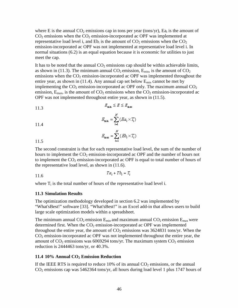
46

where E is the annual CO2 emissions cap in tons per year (tons/yr), Eai is the amount of CO2 emissions when the CO2 emission-incorporated ac OPF was implemented at representative load level i, and Ebi is the amount of CO2 emissions when the CO2 emission-incorporated ac OPF was not implemented at representative load level i. In normal situations (6.2) is an equal equation because it is economic for utilities to just meet the cap.

It has to be noted that the annual CO2 emissions cap should be within achievable limits, as shown in (11.3). The minimum annual CO2 emission, Emin, is the amount of CO2 emissions when the CO2 emission-incorporated ac OPF was implemented throughout the entire year, as shown in (11.4). Any annual cap set below Emin cannot be met by implementing the CO2 emission-incorporated ac OPF only. The maximum annual CO2

emission, Emax, is the amount of CO2 emissions when the CO2 emission-incorporated ac OPF was not implemented throughout entire year, as shown in (11.5).

11.3

11.4

11.5

The second constraint is that for each representative load level, the sum of the number of hours to implement the CO2 emission-incorporated ac OPF and the number of hours not to implement the CO2 emission-incorporated ac OPF is equal to total number of hours of the representative load level, as shown in (11.6).

11.6

where Ti is the total number of hours of the representative load level i.

11.3 Simulation Results

The optimization methodology developed in section 6.2 was implemented by “What'sBest!” software [33]. “What'sBest!” is an Excel add-in that allows users to build large scale optimization models within a spreadsheet.

The minimum annual CO2 emission Emin and maximum annual CO2 emission Emax were determined first. When the CO2 emission-incorporated ac OPF was implemented throughout the entire year, the amount of CO2 emissions was 3624831 tons/yr. When the CO2 emission-incorporated ac OPF was not implemented throughout the entire year, the amount of CO2 emissions was 6069294 tons/yr. The maximum system CO2 emission reduction is 2444463 tons/yr, or 40.3%.

11.4 10% Annual CO2 Emission Reduction

If the IEEE RTS is required to reduce 10% of its annual CO2 emissions, or the annual CO2 emissions cap was 5462364 tons/yr, all hours during load level 1 plus 1747 hours of

47

load level 2 have to be implemented with CO2 emission-incorporated ac OPF, while the remaining hours can be omitted from the OPF optimization, as shown in Figure 11.4.

Figure 11.4 10% annual CO2 emission reduction


If the IEEE RTS is required to reduce 20% of its annual CO2 emissions, or the annual CO2 emissions cap was 4855435 tons/yr, all hours during load level 1, load level 2 and load level 3, plus 22 hours of load level 4 have to be implemented with CO2 emission-incorporated ac OPF, while the remaining hours can be omitted from the OPF optimization, as shown in Figure 11.5


48


If the IEEE RTS is required to reduce 30% of its annual CO2 emissions, or the annual CO2 emissions cap was 4248505 tons/yr, all hours during load level 1, load level 2 and load level 3, plus 1495 hours of load level 4 have to be implemented with CO2 emission-incorporated ac OPF, while the remaining hours can be omitted from the OPF optimization, as shown in Figure 11.6.



If the IEEE RTS is required to reduce 40% of its annual CO2 emissions, or the annual CO2 emissions cap was 3641576 tons/yr, all hours during load level 1, load level 2, load level 3, load level 4, and load level 5, plus 678 hours of load level 6 have to be implemented with CO2 emission-incorporated ac OPF, while the remaining hours can be omitted from the OPF optimization, as shown in Figure 11.7.

49


11.8 CO2 Emission Reductions and Fuel Costs

The annual CO2 emission reduction will increase the annual fuel costs. Table 11.3 summaries the fuel costs in terms of various annual CO2 emission reduction requirements.

Table 11.3 Annual CO2 Emission Reductions and Fuel Costs

CO2 emissions (million tons/yr)

6.07 5.46 4.86 4.25 3.64

CO2 emission reduction (%) N/A 10% 20% 30% 40%

Fuel costs (million $/yr) 147.98 222.16 305.49 393.53 491.70

Fuel costs increase (million $/yr)

N/A 50.1% 106.4% 165.9% 232.3%

50

12. Conclusions and Future Work

The technique to include a price on CO2 in power system dispatch simulations has been developed and demonstrated on the modified IEEE reliability test system. Conventional economic dispatch and ac optimal power flow (OPF) studies were both run, with generation dispatch and operating costs as outputs. OPF results are significantly different from ordinary economic dispatch calculations, showing that congestion is an important consideration in CO2 emission reductions. The results further indicate that high carbon prices will be required to accomplish significant CO2 reductions using only existing generation, especially when natural gas prices are high. When the price of new generation is considered in planning studies, the lower cost and higher efficiency of combined-cycle gas-fired units, when compared to coal-fired or nuclear units, lowers the carbon price required for reductions.

The method is extended to studies of renewable energy and energy storage through time-series simulations, which allow time-varying generation and loads through any period of interest. Solar, wind, and battery storage are all simulated on daily and annual schedules. Lack of unit commitment algorithms within the OPF technique limit the usefulness of the time-series simulations, and addition of unit commitment is a future research objective. Some conclusions are still possible without unit commitment:

Renewable generation reduces CO2 emissions since it offsets fossil-fired generators in an electric power system. Fossil-fired generation, however, is still required to provide reserve capacity for the variable renewable generation. Such units still emit CO2, even if at no output. The emissions of reserve units must be considered in the overall emissions of an electric power system. Each increment of additional capacity of renewable generation installed reduces CO2 emissions. However, the change of emissions and system operating cost are not linear with renewable capacity due to complexities of the interconnected electric power system. These complexities include the renewable resource availability and variability characteristics, conventional generation characteristics (ramp rates and cost functions), transmission congestion, and the number of fossil-fired generators online as reserve units for renewables.

Wind generation has a significantly lower capacity credit than solar, because wind is more variable and less predictable than solar. Solar’s higher credit reduces the need for other reserve units, which can lower costs and emissions, and produces significantly different results between solar and wind generators. Any energy generated by wind or solar generators is almost always purchased by the power system, so CO2 prices have no effect on the operation of installed wind and solar generation. A price on CO2 does, however, provide an incentive to build new solar and wind generators, because increased generating costs from fossil-fired generators results in higher payments to renewable generators.

Energy storage is traditionally dispatched to minimize operating cost over a daily or weekly period, which results in its being charged off-peak and discharged on-peak. This tends to increase CO2 emissions because the storage is charged by coal-fired generation and offsets gas-fired generation at discharge. New storage control algorithms are needed to dispatch storage for CO2 or other emission reduction.

51

The techniques developed can be realized in commercial or research software or developed as a stand-alone application, and has potential to be utilized for investigating and assessing the effects, including costs and reliability, of GHG limits on the electric power industry.

A verified model of the Western Electricity Coordinating Council (WECC) system, with additional detail in California, is almost ready for use. The techniques developed in this project will be applied to the California system to study how existing and new generation, transmission, and storage can be operated to reduce carbon emissions.

52

References

[1] Intergovernmental Panel on Climate Change (IPCC), “Climate Change 2007: Synthesis Report”, 2007, www.ipcc.ch/

[2] Intergovernmental Panel on Climate Change (IPCC), “Climate Change 2007: The Physical Science Basis”, 2007, www.ipcc.ch/

[3] National Oceanic and Atmospheric Administration (NOAA), “State of the Climate Report”, 2007, lwf.ncdc.noaa.gov/oa/climate/research/2007/dec/dec07.html

[4] National Aeronautics and Space Administration (NASA), “GISS Surface Temperature Analysis”, 2007, data.giss.nasa.gov/gistemp/2007/

[5] Energy Information Administration, “Greenhouse Gases, Climate Change and Energy”, May 2008, ww.eia.doe.gov/bookshelf/brochures/greenhouse/Chapter1.htm

[6] Energy Information Administration, “Annual Energy Outlook 2008: With Projections to 2030”, June 2008, www.eia.doe.gov/oiaf/aeo/

[7] Morgan, G., Lave, L., and Apt, J., “The US Electric Power Sector and Climate Change Mitigation,” Pew Center on Global Climate Change, June 2005, www.pewclimate.org/docUploads -/Electricity%5FFinal%2Epdf

[8] Goodman, S., Walker, M., “Benchmarking Air Emissions of the 100 Largest Electric Power Producers in the United States – 2004”, www.nrdc.org/air/pollution/benchmarking/

[9] Energy Information Administration (EIA), “U.S. Dep’t of Energy, U.S. Data Projections, Forecast & Analyses: Carbon Dioxide Emissions by Sector and Source tbl. 18”, March 2008

[10] Energy Information Administration, “Electric Power Monthly”, June 2008, www.eia.doe.gov/cneaf/electricity/epm/epm_sum.html

[11] United Nations Framework Convention on Climate Change, "Kyoto Protocol: Status of Ratification", May 2008

[12] Kyoto Protocols to the United Nations Framework Convention on Climate Change, “United Nations Framework Convention on Climate Change, United Nations”, 1998, unfccc.int/resource/docs/convkp/kpeng.pdf

[13] United Nations Framework Convention on Climate Change, “The Mechanisms under the Kyoto Protocol: Emissions Trading, the Clean Development Mechanism and Joint Implementation”, unfccc.int/kyoto_protocol/mechanisms/items/1673.php

[14] European Commission, “EU action against climate change: leading global action to 2020 and beyond”, 2007. www.europa-eu-un.org/documents/en/070531_eu_action_against_climate_change.pdf

[15] European Commission, “EU action against climate change: EU emissions trading – an open scheme promoting global innovation”, Sep. 2005, ec.europa.eu/environment/climat/pdf/emission_trading2_en.pdf

[16] Bureau of Oceans and International Environmental and Scientific Affairs Global, “Climate Change Initiative”, 2002, www.state.gov/g/oes/rls/fs/2002/12956.htm

[17] Regional Greenhouse Gas Initiative (RGGI), www.rggi.org/about.htm [18] Western Governors’ Association, “Clean Energy, a Strong Economy and a Health

Environment”, June 2006 [19] Energy Information Administration, “Emissions of Greenhouse Gas in the United

States 2006”, www.eia.doe.gov/oiaf/1605/ggrpt/

53

[20] Energy Information Administration, www.eia.doe.gov/fuelelectric.html [21] Energy Information Administration, “Table F17: Nuclear Consumption, Price and

Expenditure Estimates, 2006,” 2006, www.eia.doe.gov/emeu/states/sep_fuel/html/fuel_nu.html

[22] Intergovernmental Panel on Climate Change (IPCC), “2006 IPCC Guidelines for National Greenhouse Gas Inventories,” 2006, www.ipcc-nggip.iges.or.jp/public/2006gl/index.html

[23] California Renewable Portfolio Standard, “Renewable Generation Integration Cost Analysis: Phase III: Recommendation for Implementation,” California Energy Emissions, July 2004

[24] Goel, L.; Aparna, V.P.; Peng Wang, "A Framework to Implement Supply and Demand Side Contingency Management in Reliability Assessment of Restructured Power Systems," Power Systems, IEEE Transactions on , vol.22, no.1, pp.205-212, Feb. 2007

[25] California Independent System Operator, “Incorporation of Wind Power Resources into California Energy Market,” 2005, www.caiso.com/docs/2003/01/29/2003012914230517586.html

[26] Piyasak Poonpun and Ward Jewell, “Analysis of the Cost per Kilowatt Hour to store Electricity,” IEEE Transactions on Energy Conversion, Vol.23, No. 2, June 2008

[27] ERCOT, “Planning and Operations Information,” planning.ercot.com/ [28] ERCOT, “Hourly Load Data Archives,” www.ercot.com/gridinfo/load/load_hist/ [29] ERCOT, “Distributed Generation Task Force,” November 5, 2007,

www.ercot.com [30] Piyasak Poonpun, Effects of New Low Carbon Emission Generators and Energy

Storage on Greenhouse Gas Emissions in Electric Power Systems, PhD Dissertation, Wichita State University, 2009.

[31] Grigg, C, etc., "The IEEE Reliability Test System-1996. A report prepared by the Reliability Test System Task Force of the Application of Probability Methods Subcommittee," Power Systems, IEEE Transactions on , vol.14, no.3, pp.1010-1020, Aug 1999.

[32] Wayne L. Winston, Operations Research: Application and Algorithms, 4th ed., Duxbury Press, 2003.

[33] “What’s Best”, Software Package, Ver. 9.0, Lindo Systems, www.lindo.com/index.php?option=com_ content&view=article&id=3&Itemid=11.

54

Project Publications

Miaolei Shao, The Effects of Greenhouse Gas Limits on Electric Power System Dispatch and Operations, PhD Dissertation, Wichita State University, September 2008.

Miaolei Shao, Ward Jewell, The Effects of Greenhouse Gas Limits on Electric Power System Dispatch and Operations, 2008 Frontiers of Power Conference, Oklahoma State University, October 2008.

Piyasak Poonpun, Effects of Low Carbon Emission Generation and Energy Storage on Greenhouse Gas Emissions in Electric Power Systems, PhD Dissertation, Wichita State University, 2009.

Miaolei Shao, Ward Jewell, CO2 Emission-Incorporated AC Optimal Power Flow and Its Primary Impacts on Power System Dispatch and Operations, 2010 IEEE PES General Meeting, Minneapolis, July 2010.

PART 2

The Impact of Alternative GHG Regulation on the Performance of Congested Electricity Markets in the Presence of Strategic Generators and Demand

Response

Shmuel S. Oren

Anthony Papavasiliou

Tanachai Limpaitoon

University of California at Berkeley

Yihsu Chen

University of California Merced

Information about Part 2

For information about Part 2 contact: Shmuel Oren The Earl J. Isaac Professor Department of Industrial Engineering and Operations Research 4141 Etcheverry Hall University of California at Berkeley Berkeley, CA 94720 Phone: (510)642-1836 FAX: (510)642-1403 Email: [email protected] Power Systems Engineering Research Center




2010 University of California, Berkeley. All rights reserved.

i

Table of Contents

1.Introduction ...................................................................................................................... 1

2.Strategic Generator’s Behavior and Demand Elasticity Matter ....................................... 3

3.Three Bus Model.............................................................................................................. 5

3.1RPS Policy ................................................................................................................ 6

3.2Taxing ....................................................................................................................... 8

4.Results .............................................................................................................................. 9

4.1Unconstrained Equilibrium ....................................................................................... 9

4.2Pollution Constrained Equilibrium ........................................................................... 9

4.3Transmission Constrained Equilibrium................................................................... 10

5.Examples ........................................................................................................................ 13

5.1Full Example ........................................................................................................... 13

5.2The effect of RPS (f) and taxing (t) on firm strategies ........................................... 15

5.3An Example of Gaming RPS .................................................................................. 16

6.Equilibrium Analysis under Cap and Trade ................................................................... 20

6.1The Equilibrium Model ........................................................................................... 20

6.2The GHG-Incorporated Equilibrium Model ........................................................... 22

7.Model Calibration .......................................................................................................... 25

8.Economic Analysis ........................................................................................................ 28

8.1Scenario Assumptions ............................................................................................. 28

8.2Economic Analysis.................................................................................................. 29

9.Conclusions .................................................................................................................... 35

10.References .................................................................................................................... 36

ii

List of Figures

Figure 2.1 Perverse Effect of CO2 Tax in the Presence of Demand Elasticity, Congestion, and Strategic Generators ..................................................................................................... 3

Figure 3.1 Three node dc lossless network ......................................................................... 5

Figure 5.1 Welfare and deadweight loss in the oligopolistic market ................................ 14

Figure 5.2 Profits in the oligopolistic market ................................................................... 14

Figure 5.3 The equilibrium parametric on f and t. ............................................................ 16

Figure 5.4 An example where RPS pricing results in underutilization of transmission capacity. ............................................................................................................................ 17

Figure 5.5 Generation as a function of K for the third example ....................................... 18

Figure 5.6 Price at the load and as a function of K for the third ....................................... 19

Figure 7.1 Power outputs by fuel types against different CO2 prices ............................... 26

Figure 7.2 Plot CO2 emission and production costs against different CO2 prices ............ 27

Figure 8.1 Power outputs at loose cap level (=1,205 tons) ............................................... 33

Figure 8.2 Power outputs at moderate cap level (=815 tons) ........................................... 33

Figure 8.3 Power outputs at extreme cap level (=515 tons) ............................................. 34

iii

List of Tables

Table 5.1 PTDF for the symmetric three node network of the first example ................... 13

Table 5.2 Prices and production levels for duopoly ......................................................... 14

Table 7.1 Generation unit properties in the 24-bus test case ............................................ 26

Table 8.1 Scenario descriptions ........................................................................................ 29

Table 8.2 Economic surpluses (in thousands) ................................................................... 29

Table 8.3 Summary of comparative statistics: Loose cap level (=1,205 tons) ................. 31

Table 8.4 Summary of comparative statistics: Moderate cap level (=815 tons) ............... 31

Table 8.5 Summary of comparative statistics: Extreme cap level (=515 tons) ................ 32

iv


1

1. Introduction

The United States are moving fast towards regulating greenhouse gas (GHG) emissions. The electricity sector accounted for 40.6% of US energy consumption in 2007 and 70% of this energy was supplied by fossil fuel energy sources, namely natural gas, coal and oil. Therefore, the regulation of emissions is expected to have a major impact in the electric power industry.

One way of reducing GHG emissions is by promoting renewable generation. Due to the high long-run average costs of these resources, as well as the costs resulting from their variable and nondispatchable nature, regulatory intervention is required for integrating a significant capacity of these resources. For example, coal fired generation typically costs less than gas fired generation which costs less than renewable resources such as wind power and solar power. Therefore, introducing these resources at a large scale in power systems will inevitably impact the wholesale price of electricity, as well as electric power production costs and the distribution of social surplus [1]. It is also possible that emissions regulations will affect the strategic interaction between power generating firms, enhancing the market power of certain producers in the expense of others.

In this section we examine three policies for regulating emissions by promoting renewable energy: renewable portfolio standards (RPS) taxing of emissions and a cap and trade approach. RPSs require that a certain fraction of the energy which is generated or sold within a state be generated by renewable energy sources other than hydro power, such as wind, solar or geothermal power [1]. In some states, suppliers are allowed to purchase RECs (renewable energy credits) to fulfill their obligation. As of June 2007, RPS is implemented in more than half of the US states. For example the RPS targets in California require that 20 % of the energy sales originate from clean energy sources [2]. Unlike RPS which directly stipulates a requirement for electricity mix, taxes target emissions by making polluting technologies less competitive. Sweden, Denmark, Finland and Norway have CO2 taxes with tax rates ranging widely [3]. For example, the Swedish tax rate is currently around 70$/ton while Norway rates differ for different sectors ranging from 12 to 47$/ton.

The analysis of the impacts induced by alternative regulatory mechanisms is complicated by the presence of a transmission network. The effect of transmission constraints on strategic interactions in transmission networks have been studied extensively but the research on the impact of emissions regulation in power markets mainly consists of empirical studies [4,5], with the exception of Chen and Hobbs [6]. In their work, Chen and Hobbs modeled how generators could manipulate the power market by using NOx emissions permits. In the spirit of [7] and [8] who focus on small scale networks in order to gain insight on firm interactions, we first focus on a three node network and derive analytic results that shed light on the impacts of emissions policies on nodal prices and generator output in a congested network with strategic generators.

There is an increasing consensus for the implementation of emissions trading in many US states. For example, California Assembly Bill 32 will mark the launch of an emissions trading program in California with the objective of reducing GHG emissions to 1990 levels by 2020. We study the implication of a Cap and Trade approach in the presence of

2

congestion and strategic generators’ behavior using an equilibrium model applied to an IEEE 24 Bus test case.

The analysis in this section complements the work presented in other parts of this report which emphasizes the accurate modeling of AC network characteristics but ignores strategic generators’ behavior and demand response by assuming that the market is perfectly competitive and can be simulated by means of an Optimal Power Flow (OPF) model while the demand is inelastic. By contrast we employ an equilibrium model of an oligopolistic market where generators behave strategically so as to maximize firms’ profits while the demand responds to prices. To make such a model computationally tractable we must employ a DC approximation of the network. We validate this approximation by comparing the AC OPF results for emissions and generators output obtained for an IEEE 24 bus test case with the corresponding results obtained from a DC approximation under perfect competition.

3

2. Strategic Generator’s Behavior and Demand Elasticity Matter

When externalities of carbon emissions are imposed on firms by permits (quantity) or taxes (prices), firms will face higher energy generation costs. They will alter their production schedules by considering heterogeneity in both fuel and emissions costs. This change in outputs from plants in different locations might alleviate transmissions congestion and alter congestion patterns, possibly leading to some unintended consequences under the framework of Locational Marginal Prices (LMPs). For example, it has been shown by Downward [11] that when coal firms are subject to a CO2 tax, cleaner firms can behave in a more competitive manner. Depending on the location of plants, this could lead to no congestion, thereby reducing overall LMPs. As a result, energy consumption can increase, which lead to an increase in overall CO2 emissions compared to no tax case. We reproduce this example in Figure 2.1, below.

Figure 2.1 Perverse Effect of CO2 Tax in the Presence of Demand Elasticity, Congestion, and Strategic Generators

We note that in the absence of a Carbon tax (top panel) the “dirty” generator at node 1 is significantly cheaper that the “clean” generator at node 2. This results in the connecting line being congested due to imports from the cheap to the expansive node. However, the congestion splits the market and facilitates two local monopolies which result in loctional marginal prices of $102/MWh and $119/MWh, significantly above the corresponding marginal costs of $40/MWh and $50MWh. Imposing a carbon tax of $26 per ton increases the marginal cost of the dirty generator to $66/MWh making it more expansive than the clean generator whose marginal cost is only $60.4/MWh. As a result the export from node 1 to node 2 goes down so that the connecting line is no longer congested and the two nodal markets merge into a single duopoly market. The increased competition causes the prices (which are now identical at both nodes) to drop to $100/MWh and since demand is price-responsive the total load increases from 335MW to 381MW and social

4

welfare increases by $2377/h. Unfortunately the increase in consumption also increases total CO2 emissions by 5 ton/h. In summary, a carbon tax which under perfect competition would reduce consumption and shift production so that emissions are reduced, achieves the opposite result when strategic generators’ behavior and demand response are taken into consideration. While this example may represents an extreme theoretical market anomaly which may not be very prevalent in practice, it highlights the need to consider the intricate interactions and the potential for unexpected consequences which motivates the analysis in this section of the report.

Unfortunately, when we account the aforementioned interactions and allow firms to deviate from their price-taking assumptions, the interactions of energy and emissions markets within a transmission-constrained network becomes difficult to predict. Unlike the perfectly competitive outcome which can be simulated by solving a single OPF problem, an equilibrium model with multiple players behaving strategically is computationally much more demanding. Furthermore, under perfect competition, carbon costs are directly reflected in the LMPs through firms’ marginal energy costs. Under tradable permits, changes of a firm’s output not only affect its marginal cost, but also affect other firms’ marginal (abatement) costs since the permits price would likely be changed as well. Moreover, even if the congestion component of the LMPs may decline with the contraction of outputs by oligopoly produces, the emissions level will not increase since it is capped. So, change in permit price could affect produces in very different ways. This motivates us to perform a more thorough analysis exploring the implications of a GHG permit trading regulation on various economic indicators, equilibrium prices, and ownership structure.

5

3. Three Bus Model

Our analysis in this subsection focuses on a three-node power network, the simplest setting that still allows us to examine the interactions between transmission and environmental regulations by deriving closed form solutions for the output of the generators and for nodal prices. Due to the symmetry of the network which we are considering, without loss of generality we assume that a clean generator is located in node 1, a polluting generator in node 2 and load in node 3 as shown in Figure 3.1. Consistent with our presumption that nonpolluting generators are typically more expensive than conventional generators, we will assume that the generators in the three-node network have a constant marginal cost ��, with �� . The inverse demand function at the node i is assumed to be linear, given by the following expression: �� .

Figure 3.1 Three node dc lossless network

Our formulation assumes the transmission network is operated by a welfare maximizing independent system operator (ISO), similar to [9]. The electricity market is simulated as a Cournot game, whereby generators compete in the quantity of their output. Generators bid a quantity of power to be sold at the node in which they are located, and are rewarded the nodal price at their location. The ISO arbitrages any non-cost based difference in the locational price of electricity and clears the market with the objective of maximizing social welfare subject to the operational constraints of the network. We subsequently demonstrate that this formulation is equivalent to a Cournot competition in quantities with additional constraints imposed by both emissions regulation as well as the capacity constraints of the network transmission lines. As in the case of classical Cournot competition, generators decide simultaneously about their output whereas the nodal price is determined by their joint decision.

We assume that generators do not anticipate the effect of their decisions on the locational pricing of electricity by the ISO. In other words, generators behave as price takers in

�Nonpolluting generator at node 1�Polluting generator at node 2�Load at node 3�Constant marginal costs � Linear demand

3( )P q a bq= −

~

~

Clean

Dirty

LOAD

Node 1

Node 2Node 3

G1

G2

6

transmission services [10]. To exemplify this assumption, a generator, which is charged for congesting the network cannot anticipate that by slightly reducing output it can decongest the grid and avoid paying a price for scarce transmission.

3.1 RPS Policy

Increase the penetration of renewable energy sources in the supply mix is expected to increase the overall cost of supplying power. These additional costs are born by generators and propagated to some extent, through prices, to consumers. In order to capture this effect in our model, we have assumed that the RPS goal is imposed as an operational constraint in the ISO’s optimization problem. Hence, the RPS policy is included in the ISO optimization problem explicitly, and emissions are priced in a similar fashion to transmission services. In the ISO problem, the RPS constraint requires that the proportion of energy that is supplied by firms, which use polluting fuels cannot exceed a specified fraction f of the total energy supply. This is equivalent to setting an RPS requirement of 1− f, i.e. requiring that the fraction of power supplied by nonpolluting sources exceeds 1− f. The ISO optimization problem is summarizes as follows: max��

� ��

��

�. �. � �� 0 ��

� �,�� !

� �,�� !

∑ �� #�� 0 �$�

We denote N the set of nodes and L the set of arcs. The goal of the ISO is to regulate flows in the network in order to maximize social welfare W. The ISO decision variables are ri, the quantities of power imported from node i to the hub node (negative for export). The hub node is chosen arbitrarily as the load node, namely node 3. Pi is the nodal price. The first constraint in the problem is a mass-balance constraint which requires that the ISO is neither a net producer nor a net consumer of energy. The second and third constraints ensure that the network transmission constraints are satisfied. In these constraints, Kl denotes the capacity limit of line l and Dl,i denotes the power transfer distribution factor (PTDF) between line l and node i, the exact meaning of which is explained in the next paragraph. The last constraint is the RPS constraint imposed on the operation of the network, whereby the output of polluting generators cannot exceed a fraction f of total output. In this constraint, di is an indicator parameter equal to 1 if the firm located at node i operates a polluting generator, and 0 otherwise. The symbols in parentheses denote the Lagrange multipliers of the ISO problem, which will be used subsequently for pricing electricity. Capacity constraints on the output of generators can be included in the problem, but have been omitted since they do not add insight to the current analysis.

We use a DC-approximation of Kirchhoff’s Laws to model power flow in the network by PTDFs. The entry Dl,i in the PTDF matrix specifies the proportion of power which flows through line l when a unit of power is being transmitted from the hub to node i. For

7

example, D1−2,2 =0.8 implies that if 1 MW of power were to flow from node 2 to the hub (node 3), 0.8 MW would flow through line 1-2.

Prices act as a mechanism by which the ISO can signal or direct generators to either increase or reduce their output in order to satisfy the operational constraints of the system. This is clarified by the following first order necessary conditions (KKT conditions) of the ISO problem, where the symbol ⊥ indicates complementarity between variables and their corresponding constraints (x⊥y can be interpreted as x orthogonal to y) �� % �� &� '� � 0, )* + ∑ �� 0 &� �� ,� ��,�� , )* +

'� � $�# �� 0 � �� , � �,�� % � - 0, )� !��

0 � �� , � �,�� % � - 0, )� !��

0 � $ , ∑ �� #�� 0��

From the above ISO first-order conditions we obtain the congestion and pollution rents which are imposed in the various nodes of the network. The congestion rents φi =(λ+ −

λ−)Dl,i are equal to the marginal value of the congested transmission lines weighted by the extent to which a generator utilizes the congested lines. These rents will be negative (i.e. costs) whenever a generator contributes to the congestion of a line, and positive (i.e., revenues) otherwise. Similarly, pollution rents are given by the expression '� � $�# ��. These rents reward nonpolluting producers and penalize polluting generators whenever the RPS constraint is binding.

According to our model assumptions, firms correctly anticipate the output levels of their rivals and the impact of their actions on price at the load node but they act as price takers in transmission services and pollution charges. Therefore, whereas the price p is endogenous to the firms optimization problems, both congestion and pollution rents φ and ψ are exogenous to these problems. The firm optimization problem is therefore given by the following: .�: max��

�� % &� % '��

s.t. 0 � ��

The second constraint in the above optimization problem defines implicitly the relation between qi and p which plays a role similar to a residual demand function is a standard Cournot model.

Given our formulation, the price at the location of a generator can be obtained by adding pollution and congestion rents to the hub price. This allows us to treat the competition between generators as a constrained Cournot game where firms need to additionally satisfy transmission and emissions constraints.

( ) ( )1

,j ji

j N j N j ij jq P p qψϕ

−

∈ ∈ ≠

= + −+∑ ∑

8

3.2 Taxing

The alternative policy, which we consider, taxing, is readily incorporated in the model. We assume that polluting generators are levied with an amount t per MWh of output, which is not imposed to renewable generators. Therefore, the ISO does not include emissions regulation as an operational constraint in its optimization problem: max��

� ��

��

�. �.� �� 0 ��

� �,�� !

� �,�� !

As in the case of RPS, we derive the KKT conditions of the ISO problem which will be necessary for obtaining closed form solutions subsequently. �� % �� &� '� � 0, )* + ∑ �� 0 &� �� ,� ��,�� , )* +

0 � �� , � �,�� % � - 0, )� !��

0 � �� , � �,�� % � - 0, )� !��

The tax enters the model formulation only in the optimization problems of the firms: .�: max�� % &�� %��

s.t. 0 � ��

( ) ( )1

,j ji

j N j N j ij jq P p qψϕ

−

∈ ∈ ≠

= + −+∑ ∑

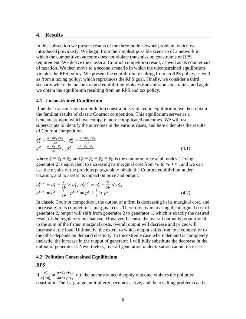
9

4. Results

In this subsection we present results of the three-node network problem, which we introduced previously. We begin from the simplest possible scenario of a network in which the competitive outcome does not violate transmission constraints or RPS requirement. We derive the classical Cournot competition result, as well as its counterpart of taxation. We then move to a second scenario in which the unconstrained equilibrium violates the RPS policy. We present the equilibrium resulting from an RPS policy, as well as from a taxing policy, which reproduces the RPS goal. Finally, we consider a third scenario where the unconstrained equilibrium violates transmission constraints, and again we obtain the equilibrium resulting from an RPS and tax policy.

4.1 Unconstrained Equilibrium

If neither transmission nor pollution constraint is violated in equilibrium, we then obtain the familiar results of classic Cournot competition. This equilibrium serves as a benchmark upon which we compare more complicated outcomes. We will use superscripts to identify the outcomes in the various cases, and here c denotes the results of Cournot competition. ��

�� , ��

�� , �� (4.1)

where and is the common price at all nodes. Taxing generator 2 is equivalent to increasing its marginal cost from to , and we can use the results of the previous paragraph to obtain the Cournot equilibrium under taxation, and to assess its impact on price and output. �� % �

�� 0 �� , �� , ��

�� , �� % �� 0 �� . (4.2)

In classic Cournot competition, the output of a firm is decreasing in its marginal cost, and increasing in its competitor’s marginal cost. Therefore, by increasing the marginal cost of generator 2, output will shift from generator 2 to generator 1, which is exactly the desired result of the regulatory mechanism. However, because the overall output is proportional to the sum of the firms’ marginal costs, overall output will decrease and prices will increase at the load. Ultimately, the extent to which output shifts from one competitor to the other depends on demand elasticity. In the extreme case where demand is completely inelastic, the increase in the output of generator 1 will fully substitute the decrease in the output of generator 2. Nevertheless, overall generation under taxation cannot increase.

4.2 Pollution Constrained Equilibrium

RPS

If ��

��

�� 0 # the unconstrained duopoly outcome violates the pollution

constraint. The La-grange multiplier µ becomes active, and the resulting problem can be

10

treated as a Cournot duopoly with modified marginal costs and where the generators obey the additional constraint. ��

� � �� % �� 0 �� , ��

� � �� % �� , �� % ��

�� , �� % ��

� 0 �� , �� % ��

� � �� , ��

� (4.3)

where the superscript p refers to the equilibrium when pollution constraint is binding. It follows from the closed form expression of ψ1 and ψ2 (which we do not present here) that the nodal price and the output at node 1 will increase and the opposite will be true for node 2. If f< 0.5 the pollution constraint will certainly be binding because in the unconstrained equilibrium q1<q2. From the closed form expressions of ψi we can also conclude that for f<0.5 the total output will be less than the unconstrained output because the reduction in polluting generation is not fully compensated by an increase in clean generation. The opposite will be true when f>0.5.

Overall, it is clear that RPS enhances the profitability of generator 1 at the expense of generator 2. The impact on load prices depends on the specific value of f, and for stringent regulations (f<0.5) price at the load increases, whereas for less stringent regulations price at the load decreases due to a dampening in the market power of generator 2.

Taxing

In order to compare RPS with taxing on an objective basis, we consider the particular case where the tax t results in the RPS requirement

�� #. The tax �� for which this

equilibrium holds is given by the following equation: ��

�� , (4.4)

where the relevant quantities are indexed by superscript f. By substituting the closed form

of $ � ��in equations 3 and the closed form of �� into equations 2 we obtain the

following inequalities which can be used to compare the two policies: ��

� � ��, ��

� � ��, �� 0 ��

�, �� 0 ��. (4.5)

We can see that both generators will reduce their output. The reason is that taxing, unlike RPS, does not offer sufficient incentives to generator 1 for increasing its output. As a result, electricity price at demand node increases, which is an undesirable side effect of this regulation.

4.3 Transmission Constrained Equilibrium

In this section it is assumed that the unconstrained equilibrium violates one or more transmission constraints. In the spirit of traditional literature on market power in

11

electricity networks, this section focuses on investigating how constraints influence the market power of generators.

RPS

We will consider a symmetric network, in which all transmission lines have the same impedance and capacity. Because power flow along a route is inversely proportional to the impedance of the route, one third of the power produced by each generator follows the short path to the load and the remaining two thirds follow the long path. Generator 2 produces at lower marginal cost, hence its output would be greater in an unconstrained network. Therefore, the first line to become congested will be line 2−3. This problem is equivalent to a Cournot duopoly where the marginal cost of generator I is �� '� under

the additional constraint �� % �

� �� , where &� = ��,�� 0 is the transmission

charge at node i. Solving the corresponding system of equations we obtain the following closed form expressions: �� % ��

�� , �� % �� , �� % ��

�� , �� % �� , �� % ��

� � �� , �� 0 �� (4.6)

The congestion charges for generator 2 are twice as large as for generator 1, φ2 =2φ1, because it contributes twice the flow in the congested line, compared to its competitor. In summary, generator 2 produces a smaller output at a lower price compared to the unconstrained duopoly, whereas generator 1 produces the same output at a higher price. The overall output is reduced, therefore the price at the load increases.

It is also possible that the equilibrium is simultaneously binding in both the transmission

and the pollution constraint (if ��

��0 #). The outcome can then be obtained by

modifying the marginal costs of the generators by �� 1� '� and adding the additional constraints that

�� # and � �,�� where l is the index of the congested line. In

contrast to previous cases, the closed form solutions do not allow us to draw any general conclusion about how this outcome compares to the outcome of an unconstrained Cournot duopoly, therefore at this point we only present the resulting closed form solutions and defer to the examples for providing specific interpretations about the influence of simultaneous congestion and pollution constraints on firm strategies. ��

�,� � �� % �� , ��

�,� � �� % �� , ��,� � �� % ��

�� , ��,� � �� % ��

� , ��,� � �� % ��

� , ��,� � �� % �� (4.7)

Taxing

When taxed firms operate under binding transmission constraints, we obtain the closed form solutions by modifying the marginal cost of generator 2 to c2−t and adding the

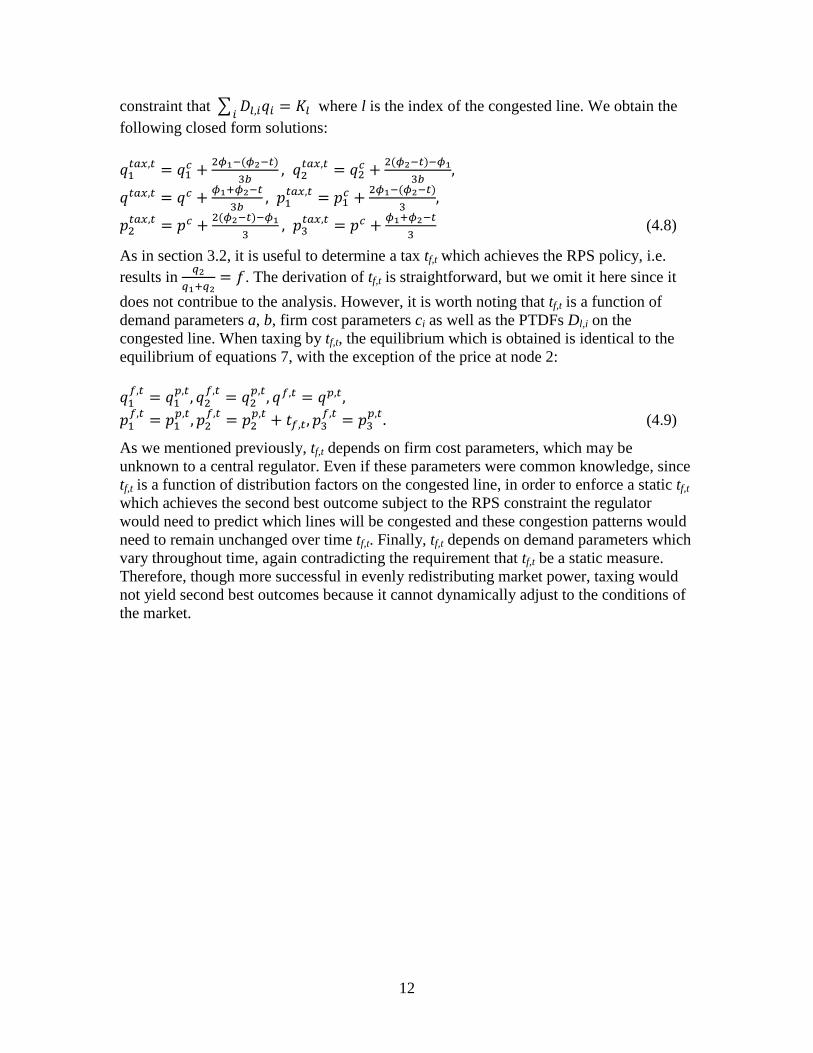
12

constraint that � �,�� where l is the index of the congested line. We obtain the following closed form solutions: ��

��,� � �� % �� , ��

��,� � �� % �� , ��,� � �� % ��

�� , ��,� � �� % ��

� , ��,� � �� % ��

� , ��,� � �� % ��

� (4.8)

As in section 3.2, it is useful to determine a tax tf,t which achieves the RPS policy, i.e. results in

��

� #. The derivation of tf,t is straightforward, but we omit it here since it

does not contribue to the analysis. However, it is worth noting that tf,t is a function of demand parameters a, b, firm cost parameters ci as well as the PTDFs Dl,i on the congested line. When taxing by tf,t, the equilibrium which is obtained is identical to the equilibrium of equations 7, with the exception of the price at node 2: ��

�,� � ��,�, ��

�,� � ��,�, ��,� � ��,�, ��

�,� � ��,�, ��

�,� � ��,� % ��,�, ��

�,� � ��,�. (4.9)

As we mentioned previously, tf,t depends on firm cost parameters, which may be unknown to a central regulator. Even if these parameters were common knowledge, since tf,t is a function of distribution factors on the congested line, in order to enforce a static tf,t which achieves the second best outcome subject to the RPS constraint the regulator would need to predict which lines will be congested and these congestion patterns would need to remain unchanged over time tf,t. Finally, tf,t depends on demand parameters which vary throughout time, again contradicting the requirement that tf,t be a static measure. Therefore, though more successful in evenly redistributing market power, taxing would not yield second best outcomes because it cannot dynamically adjust to the conditions of the market.

13

5. Examples

In this subsection we present three examples. The first example is the solution to a symmetric three node network, which confirms various conclusions which we drew in the previous section. In the second example we examine the sensitivity of optimal firm strategies on the regulatory parameters t and f which were introduced earlier. In the third example we demonstrate that emissions regulations might be vulnerable to gaming by providing an example of a nonpolluting generator which manipulates regulations in order to limit the participation of its polluting competitor in the local power market.

5.1 Full Example

We solve an example with a symmetric network. The PTDF matrix of the network is given in table 5.1. The inverse demand function is P(q) = 70 − 0.2q. The marginal costs are c1 = 30$/MWh, c2 = 20$/MWh.

Table 5.1 PTDF for the symmetric three node network of the first example

The results of the duopoly equilibria are shown in Figures 5.2-5.3 (social surplus) and Table 5.2 (prices and production levels), where the first case refers to an unconstrained system; the second case refers to a system with a thermal limit of K=75MW for each line; the third case refers to a system with a pollution constraint of f=0.2and transmission constraints of K=75MW; the last case refers to a system where taxing is enforced on generator 2. 5.2 indicates that under transmission constrained operation (Case 2), generator 2 is forced to reduce its output in order to decongest transmission line 2− 3, and prices at the load increase. Generator 1 is not affected by the transmission constraints and maintains the same output as in the unconstrained equilibrium. Also shown in Table 5.2, the price at node 2 drops in Case 3, and the price at node 1 increases where the output shifts from generator 2 to generator 1. Since the RPS requirement is less than 0.5, the price at the load is higher because the overall output decreases. From section 1.4.2, the tax for achieving the goal f = 0.2 is tf=23.3$/MWh. This leads us to consider Case 4, where we implement a tax to reproduce the RPS goal of Case 3. Table 5.2 suggests that the output of each generator decreases and the price at the load increases at a higher level than the resulting load price from RPS. From Figure 5.3 it is clear that this policy is more balanced in terms of redistributing profits compared to RPS, nevertheless deadweight loss (Figure 5.2) – mainly consumer surplus – is greater. This can be attributed to the significant reduction of total output.

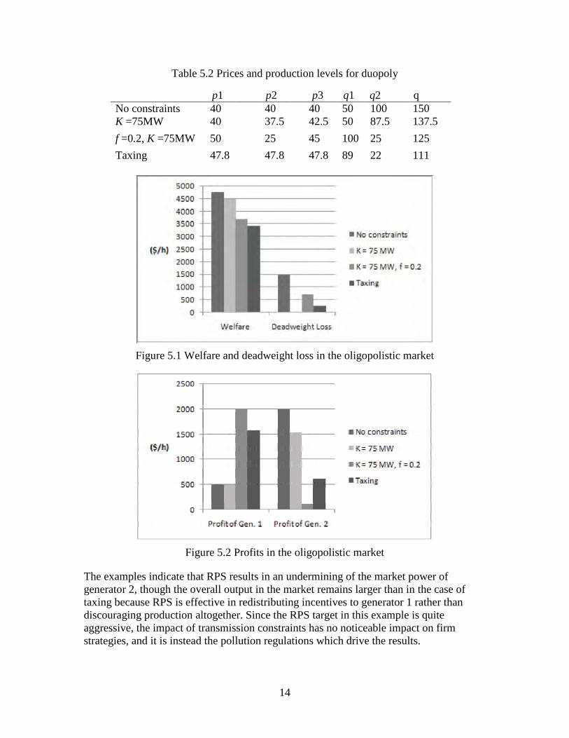
14

Table 5.2 Prices and production levels for duopoly

Figure 5.1 Welfare and deadweight loss in the oligopolistic market

Figure 5.2 Profits in the oligopolistic market

The examples indicate that RPS results in an undermining of the market power of generator 2, though the overall output in the market remains larger than in the case of taxing because RPS is effective in redistributing incentives to generator 1 rather than discouraging production altogether. Since the RPS target in this example is quite aggressive, the impact of transmission constraints has no noticeable impact on firm strategies, and it is instead the pollution regulations which drive the results.

p1 p2 p3 q1 q2 q No constraints 40 40 40 50 100 150 K =75MW 40 37.5 42.5 50 87.5 137.5

f =0.2, K =75MW 50 25 45 100 25 125

Taxing 47.8 47.8 47.8 89 22 111

15

5.2 The effect of RPS (f) and taxing (t) on firm strategies

In this section we consider the effect of emissions regulations on firm strategies. We vary the parameters that characterize the two policies, f for RPS and t for taxing, in order to know how firms’ optimal output might respond to the changes. The resulting graphs are shown in Figure 5.3. We consider both the case where the network has an unlimited transmission capacity, as well as the case where all lines have a 75MW thermal limit.

In the top of Figure 5.3 we graph equilibrium strategies parameterized on f. For f < 0.5 the output of generator 1 is obviously greater; from the overlap of the two lines, we conclude that none of the transmission constraints are binding. At f = 0.5 lines 1− 3 and 2− 3 become congested and firm outputs become equal at 75MW. As f increases, the output of generator 2 dominates, and line 2−3 is now the only congested line. At f = 0.64 the pollution constraint is no longer binding, with line 2− 3 remaining congested.

In the bottom of Figure 5.3 we consider the response of equilibrium strategies to t. For t<5 $/MWh generator 2 produces most of the output and line 2−3 is congested. When the tax exceeds 5 $/MWh, line 2− 3 is no longer congested and the output of generator 2 continues to decrease up to t=15 $/MWh, at which point the output of both generators becomes equal. For t>15 $/MWh generator 1 produces most of the output without congesting the transmission lines and total output decreases as tax increases. For t=30 $/MWh generator 2 will stop producing power. Note that this tax is greater than the marginal cost of generator 2, and the reason generator 2 can continue to generate output at taxes higher than its marginal cost is the duopoly markup on the price.

16

Figure 5.3 The equilibrium parametric on f and t.

Figure 5.3 reaffirms our conclusion that generator 1 benefits greatly from RPS pricing whereas taxing results in a comparatively balanced redistribution of generator outputs. In addition, the graphs confirm the fact that generator 1 is incented to sustain a relatively higher output compared to the taxing case. In fact, total output under taxing is significantly smaller for all but a small range of parameter values in the two graphs. Finally, the effect of transmission constraints becomes noticeable for relatively large values of f and t and does not seem to benefit any one generator.

5.3 An Example of Gaming RPS

Investing in transmission is desirable from an efficiency standpoint because, with few exceptions, it leads to increased competition across the network. In the example that follows, we show how it is possible for the nonpolluting generator to offset the benefits of large line capacities by manipulating RPS in order to constrain the participation of its competitor in the local market.

17

Figure 5.4 An example where RPS pricing results in underutilization of transmission capacity.

In the network of Figure 5.4 generator 1 has an unconstrained access to the load, whereas generator 2 is connected to the load through a capacity constrained line, and there is no link between nodes 1 and 2. For sufficiently low capacity of the line 2− 3, generator 1 will be able to exercise market power at a significant extent. Since the participation of generator 2 is limited by the capacity of line 2−3, there is a large portion of the market which is anyways unreachable by generator 2 and on which generator 1 can exercise monopolistic market power by restricting output in order to boost prices. This effect is mitigated as the capacity of line 2− 3 is increased and generator 2 is allowed to penetrate in the market. However, beyond a certain value of the line capacity generator 1 will cap its own output in order to halt the penetration of generator 2 in the market via the RPS constraint. This will happen at the point where the incremental benefits for generator 1 of sustaining a high price by withholding its own output as well as that of its competitor (through the RPS constraint) exceed the incremental benefits of achieving higher revenues by supplying a higher output. The threshold of line capacity at which generator 1 exercises this form of market power is the value of K beyond which the capacity of transmission line 2− 3 exceeds the RPS-constrained output of generator 2:

.

These ideas are clarified by the graphs in Figures 5.5-5.6. In Figure 5.5 we see the output of both generators as it varies with respect to K, for both the case where RPS constraints are not enforced and the case where they are enforced. For sufficiently low values of K, specifically for K ≤ 22.2 MW, generator 1 relies on the transmission line to keep its competitor away from the market. In this region, as K increases the output of generator 1 increases in response to the increasing penetration of generator 2 in the market. At K =22.2 MW the RPS constraint becomes active and generator 1 continues increasing its output. Generator 2 also increases its output in this intermediate range of values of K, where both the RPS as well as the transmission constraint is active. However, at the threshold value of K =25MW generator 1 finally withholds output, in order to constrain the penetration of its competitor and keep prices high at the load. For any value of K greater than this threshold value the output of both generators remains fixed, therefore line capacity greater than 25MW does not contribute to enhancing competition in this market.

In Figure 5.6 we have plotted the evolution of and with respect to K. We

observe that, indeed, beyond K =25MW the RPS constraint is tight with =0.2. It

18

is worth noting that prices at the load are not necessarily greater in the case when RPS constraints are enforced, since as we have mentioned previously, RPS is effective in depressing the market power of generator 2 and incentizing generator 1 to sustain a high output. However, for large values of K generator 1 is abusing the RPS constraint and achieving a price at the load which is higher than it would have been otherwise.

Figure 5.5 Generation as a function of K for the third example

From this example, it becomes clear that RPS will require tight regulatory monitoring, in order to ensure that nonpolluting generators which have become empowered from the new market rules do not abuse these rules. We can also conclude that these regulations will achieve their desired results without leading to unintended consequences if it is ensured that there exists a sufficient population of nonpolluting generators which compete with each other, not only with polluting competitors. In particular, California resembles the configuration of Figure 5.4 as it is a net importer of polluting generation, with significant capacity of in-state renewable energy. In addition, California is pursuing aggressive emissions regulations and renewable energy standards, therefore close monitoring of the market conduct of clean suppliers will be essential.

19

Figure 5.6 Price at the load and as a function of K for the third

20

6. Equilibrium Analysis under Cap and Trade

In previous subsections, we addressed the economic and emissions implications of renewable portfolio standards and taxes using a stylized three-node system. The strength of such approach is that it allows us to solve models analytically. So, the results can be understood intuitively. However, it is unclear if the conclusion is readily applied to the tradable permit program and to what extent our DC simplification of the network biases our conclusion. In this subsection, we take advantage of the of the alternate analysis, described in previous sections of this report, based on an ACOPF model applied to an IEEE 24 bus test case. We first validate our DC approximation for that case and then expand our equilibrium modeling approach to a DC version of that IEEE 24 bus test case.

The equilibrium model introduced in this section is a variant of the model proposed by Yao et al [12] which, we first describe without GHG constraints. This model will was extended as part of this research to account for GHG constraints by 1) associating emissions with the generation facilities and 2) coupling with an emissions cap constraint. In particular, the permits price is determined endogenously within the equilibrium framework by imposing a complementarity constraint as a market clearing condition. The producers, however, treat the permit price as exogenous. In other words, producers will behave as price-takers in permit markets. The flows in the networks are governed by the Kirchhoff’s laws through Power Transfer Distribution Factors (PTDFs).

6.1 The Equilibrium Model

The equilibrium model is based on a lossless DC load flow model of a power system where flows on transmission lines are constrained by thermal capacities. The consumers are assumed to be price-takers that are represented by a price-responsive inverse demand function in each demand location. The producers consisting of Cournot (and price-taking) producers have multiple generators located at different buses that compete to sell energy to a Pool-typed market at uniform Locational Marginal Prices (LMPs) set by the Independent System Operator (ISO). In a sense, the producers are the price-taking Cournot producers while ISO sets locational prices. The firms then decide on the level of their production when facing their respective residual demand. In this model, a virtual bus is created for each additional generator for those buses with multiple generators. Each bus then has at most one generator. The PTDF is also modified accordingly to account for this change by assuming unlimited thermal capacities and lower reactance when splitting the nodes. This is purely for computational ease, which also was applied in Yao et al. [12]. In what follows, we first introduce the notation we use in the model. Subsequently, we present mathematical programs that describe the optimization problem faced by each entity.

Mathematical Notation

Let + denote the set of buses and ! be the set of transmission lines whose elements are ordered pairs of distinct buses. Let 2 be the set of firms, and +� 3 + be the set of buses where generators owned by firm 4 2 are located.

21

Parameters � Rating of transmission line � (MVA) �,� PTDFl,i on line � with respect to a unit injection at bus * and a unit withdrawal at the slack bus �� Plant *’s must-run limit (MW) �5� Plant *’s maxmal capacity (MW) �6�� MW fixed load at bus * �� Coefficient of degree 7 of plant’s production costs * ($/MWn)

Decision Variables �� MW output of plant * �� MW import/export at bus * (import = +) � System marginal energy cost ($/MW) 1� Marginal congestion cost component of bus * ($/MW) �� Shadow price of line � in the reference direction ($/MVA) �� Shadow price of line � in the opposite direction ($/MVA) Consumers

Consumers in each location j are represented by the inverse demand function as follows: �� , )8 +. The inverse demand function at each bus is assumed to be linear with a price elasticity of -0.1. Although short-run elasticities are nearly zero, this level of elasticity is consistent with empirical studies (Espey and Espey, 2004 [14]).

Independent System Operator (ISO) Model

An ISO is assumed to maximize the system-wide social surplus subject to the transmission constraints and mass-balance of power flows in the network. By controlling the imports/exports ��, the ISO can use shadow prices � of the transmission constraints as a price signal of transmission congestions to inform and deter producers from exercising market power. Define � the marginal energy cost or price at swing or reference bus and 1� the marginal congestion cost reflecting the cost contributions of the various transmission elements experiencing congestion. The Locational Marginal Price (LMP) at each bus * is then equal to � % 1�. The ISO behaves ala Bertrand with respect to transmission services as it sets the LMPs through imports/exports. Formulation

max��: �!9 : ��;��;� <��

s.t ∑ �� 0 � �,�� , )� !��

� �� ,��, )� !��

�� % �� - 0, )* +

22

Let �, ��, and ��be the Lagrange multipliers corresponding to the energy balance constraint and thermal limits, respectively. The first order necessary conditions for the ISO are:

KKT Conditions

�� % �� 1� � 0, )* + 1� �� ,� ��,�� , )* +

∑ �� 0 0 � �� , � �,�� % � - 0, )� !��

0 � �� , � �,�� % � - 0, )� !�� Firm Model

Each firm maximizes its profit equal to revenues minus fuel costs. The fuel costs of plant * as a function of MW output is defined by <�� % �� % �

� ��, )* +. (6.1)

As for revenues, the firms earn the LMPs for each unit of MWh sold in location i since they are price takers. The costs include fuel costs <�� for the total MWh sold ��=� at all buses +� at which its generators are located. Since the firms are modeled as Cournot players, firms 4 will maximize their profit as they face a residual demand curve, treating sales from other producers as fixed. Note that the residual demand constraint can also be viewed as the market clearing condition since it can be written as ∑ ��

�� % 1��. The left-hand side of the constraint is the aggregate supply, which is equal to the aggregate demand function on the right-hand side. In perfect competition, all >�’s are set to zero as firms are no longer Cournot players.

Formulation max��: �!�,"9 �� %1�� <��

s.t. �� 5�, )* +�

∑ �� % 1�� ∑ ��\�

Let >� and ?� be the Lagrange multipliers corresponding to residual demand constraint and generation limits (both capacity and must-run limits), respectively. The first order necessary conditions for the ISO are:

23

KKT Conditions

� % 1� >� $%��$��

% ?�� ?�� 0 )* +�

>�9 $$� �� % 1�� % ∑ ��

� 0, 0 � ?�� , �� - 0, )* +� 0 � ?�� , �5� �� - 0, )* +� ∑ ��

�� % 1�� 6.2 The GHG-Incorporated Equilibrium Model

The greenhouse gas (GHG) -incorporated equilibrium model is an extension of the mixed Cournot-Bertrand model that we introduce in Section 1.6.1, i.e. generation firms compete for MW quantities and take the price set by ISO as given. We assume that emissions cap regulation is enforced by the Independent System Operator (ISO), in which firms take the permit price into consideration when producing power. The emissions cap constraint is described by � .�� @, where .��A� is the emissions function of power plant * and @ is the system-wide cap level in tons. We also model CO2

emissions as a quadratic function in MW outputs to account for its nonlinearity associated with output. The emissions of power plant * as a function of MW output is then defined by

.�� B�� % B�� % �� B�� )* +,

where B��’s are the emission coefficients of plant *. In effect, the shadow price of this constraint reflects the price of emission permits that the ISO will use as a penalty mechanism to reduce the emissions level when the cap is binding. Let $ be the price of a unit emission. The ISO’s KKT condition with respect to the emissions cap constraint is

0 � $ , @ � .�� - 0,

where M is the system-wide cap level in tons. In producers’ problem, their cost component in the objective function will need to augment to include emissions costs as follows: ∑ �� % 1�� <�� $.��.

The equilibrium problem with GHG emissions cap regulation is modeled as follows:

24

GHG-Incorporated Equilibrium Conditions C& �D& % E&�F& G H& � 0, )I J (6.2) 1� �� ,� ��,�� , )* + (6.3) ∑ �� 0 (6.4) 0 � $ , @ � .�� - 0 (6.5)

0 � �� , � �,�� % � - 0, )� !�� 0 � �� , 9 �,�� % � - 0, )� !��

� % 1� >� �� $�B�� % B�� % ?�� ?�� 0, )* +�, )4 2 (6.6) >�9 �

��% ∑ ��

� 0, )4 2 (6.7)

0 � ?�� , �� - 0, )* +�, )4 2

0 � ?�� , �5� �� - 0, )* +�, )4 2 ∑ �� % 1�� (6.8)

Note that equations (6.2)-(6.4) imply equation (6.8). So, equation (6.8) can be removed. In case of perfect competition, we can obtain the competitive equilibrium by simply replacing equation (6.7) with the constraint: >� � 0, )4 2.

25

7. Model Calibration

Compared to the previous sections using full-scale AC flow under optimal power flow framework, we use DC approximation that disregards thermal losses associated with transmission lines. Ignoring transmission resistance might alter flow patterns that could lead to different congestion patterns under some network topologies [13]. However, as reported later in this section, the nodal prices under DC models are in fact quite compatible with AC models. The input parameters (demand intercepts and slopes) to the DC model are calibrated such that the adjustments will not bias either the emissions level or the MW outputs. We outline calibration procedure and report our results in this section. The cost-minimization DC power flow model is described below. As more details about 24-bus IEEE RTS could be found in previous sections, we only mentioned them briefly whenever is necessary.

GHG-Incorporated DC Power Flow Model K*7��,��,��9 <��

s.t. ∑ �� 0 (7.1) �� % �� 6��, )* + (7.2)

� �� ,�� ,�� )� ! (7.3) ∑ .�� @ (7.4) �� 5�, )* + (7.5)

This model minimizes the system-wide energy costs, while satisfying energy balance constraint (equation 7.1), fixed load consumption (equation 7.2), thermal limits (equation 7.3), emissions cap level (equation 7.4), and generation limits (equation 7.5). The fuel cost function has been described in equation (6.1). The model yields the most cost-effective way to generate MW outputs at all locations. The optimal outputs will take into account the cost of carbon permit, which is reflected by the shadow price of the emissions cap constraint in equation (6.5).

The 24-bus IEEE RTS is used as the test case. The topology of the test system has been comprehensively described in Section 2.5.1. Similar to simulation cases presented in Section 2.5.2, the 951 MW of steam oil is replaced with 951 of steam gas in order to explore the implication of GHG regulation. This would allow system more flexibly respond to different levels of cap constraint. Table 7.1 summarizes modified generator data and emissions data. The total generator capacity is equal to 3,405 MW. We employ a global derating factor to all transmission lines by a margin of 7% to account for the differences between the two models.

26

Table 7.1 Generation unit properties in the 24-bus test case

Fuel Type

Fuel Costs [$/MMBtu]

CO2 Rate [lbs/MMBtu]

Plant Sizes [MW]

# of units

Total Capacity

[MW]

Oil 12 160 20 4 80

Gas 9.09 116 12, 100, 197 11 951

Coal 1.88 210 76, 155, 350 9 1274

Hydro 0 0 50 6 300

Nuclear 0 0 400 2 800

All analyses are performed on one-hour basis. Figure 7.1 shows the total power outputs (summing over all producers) of all fuel types. A must-run level is imposed on the oil power generation because an output that is lower than this level would give the negative costs due to its heat-rate properties. As a result, the oil-fueled generation stays flat at its must-run level because oil power generation is not optimally cost-effective to produce.

Figure 7.1 Power outputs by fuel types against different CO2 prices

By imposing the emissions cap constraint in the DC OPF model, the carbon permit price can be determined endogenously by the model. That is, the permit price is equal to the shadow price of the emissions cap constraint. When there is no emissions cap (or cap is not binding), the emissions level under DC OPF is at 921 tons/h, fairly comparable to what was reported by the AC OPF. Furthermore, the sale-weighted average LMP is 16 $/MW, which is slightly lower than that of the AC OPF model, partly because the system experienced relatively less transmissions congestion. However, at CO2 prices higher than 180 $/ton, the sale-weighted average LMP is within 5% lower than that of the AC OPF model. Figure 7.2 shows that at a CO2 price of 112 $/ton, gas-fueled units begin to replace coal because the marginal cost of gas power generation is approximately 112.2

0 50 100 150 200 250 300 350 400 4500

100

200

300

400

500

600

700

800

900

CO2 Prices ($/ton)

Po

we

r O

utp

ut

(MW

)

OilGasCoal

27

$/MWh, which is cheaper than that of coal (i.e., 113 $/MWh). As expected, when CO2 price increases, total coal-fueled power generation falls accordingly. Total CO2 emissions fell as a higher permits price put a pressure on polluting-intensive coal units as shown in Figure 7.2. However, as the permit price becomes more expensive when the cap is tightened, the CO2-costs component dominates the fuel-costs component, forcing coal power generation to drop further.

Although the AC OPF model gives a lower level of CO2 price (70 $/ton) when merit order switch between gas and coal plants occurs, the two models exhibit qualitatively similar conclusions as the reduction in coal outputs differs by fewer than 5 percentage points. For instance, when the permit price increases from 0 $/ton to 180 $/ton, the reduction in MWh output of coal power generation is 52% in the AC OPF model, compared to a 47% reduction in the DC OPF model. We, therefore, conclude the AC and DC OPF produce compatible results and proceed to our oligopoly analysis in next section.

Figure 7.2 Plot CO2 emission and production costs against different CO2 prices

28

8. Economic Analysis

8.1 Scenario Assumptions

In order to quantify the impact of the interaction of energy and emissions markets in a transmission-constrained network, we perform analysis on various scenarios with different levels of emissions cap and asset ownership. To investigate the effects of binding emissions constraints on different scenarios, we present three different cap levels, i.e. loose (1205 tons, 90% of no-cap case), moderate (815 tons, 60% of no-cap case), and extreme (515 tons, 38% of no-cap case). As can be seen later in Tables 8.3-8.5, more scenarios will face a binding emissions constraint as the cap is gradually tightened. We study seven different scenarios, shown in Table 8.1 with their description. Each scenario has an equal number of plants (32) but differs by the ownership structure. In perfect competition scenario (PC-32), all firms are assumed to be perfectly competitive. (In scenario notation, the number denotes the number of firms.) So, the ownership (which firm owns what) does not lead to different market equilibria. Under the monopoly scenario (MP-1), all facilities are assumed to be owned by a single producer. The perfect competition (PC-32) and monopoly (MP-1) scenarios are used as benchmarks bounding equilibria for other scenarios. The scenarios in Table 8.1 are ranked by their competitiveness from most competitive (top) to least competitive (bottom). The five other scenarios are Nash-Cournot oligopolistic competition. They differ by their generation portfolio and ownership structure. In defining scenarios, we use N, H and G to denote nuclear (2), hydro (6), and gas (11), respectively, in which number within parenthesis denotes number of plants. We further group these technologies as clean technologies give their relative or zero emissions rates. For instance, the scenario 32F represents the most competitive Cournot case with each firm owns one facility. To explore the implications of heterogeneity of ownership and technologies, two firms are assigned to own hydro and nuclear separately. This scenario is called N/H-26. That is, one firm owns nuclear (2) and hydro (6), and the remaining 24 facilities (32-2-6 = 24) are owned by 24 firms, a total of 26 firms. We then further model the case where two clean firms (i.e., N (2) and H (6)) operate in a less competitive market by consolidating the rest of the market into two firms with a very similar portfolio. This scenario is named N/H-4. To model the extreme cases of the heterogeneity of technologies, NH/G-3 and NHG-2 pools the clean plants together and assigns the dirty plants as one firm. The only difference between these two cases is that NH/G-3 assigns all gas facilities to one additional firm.

29

Table 8.1 Scenario descriptions

Scenario Description

PC-32 Perfect competition with 32 firms in total: each firm owns one facility.

32F Oligopolistic competition with 32 firms in total: each firm owns only one facility.

N/H-26 Oligopolistic competition with 26 firms in total: two clean firms own nuclear and hydro facilities separately, each of the other 26 firms own one facility.

N/H-4 Oligopolistic competition with 4 firms in total: two clean firms own nuclear and hydro facilities separately, and other two firms own a comparable portfolio of facilities.

NH/G-3 Oligopolistic competition with 3 firms in total: one firm owns all nuclear and hydro facilities, second firm owns all gas facilities, and the third firm owns all coal and oil facilities.

NHG-2 Duopoly competition: one firm owns all clean facilities, i.e. nuclear, hydro, and gas while the other firm owns all coal and oil facilities.

MP-1 Monopoly competition: all facilities belong to only one firm.

8.2 Economic Analysis

This section summarizes the results from economic analysis. Table 8.2 displays the social surplus analysis: consumer, producer and social surplus. Tables 8.3-8.5 summarize the comparative statics, including sale-weighted LMPs, permit price, CO2 emissions, congestion rent, output-weighted CO2 emissions rate, system fuel costs, and productive inefficiencies. Figures 8.1-8.3 show the generation mixes under different cap levels. We go through them in turn.

From Table 8.2, several observations emerge. First, consumer surplus declines as the number of firms decreases or ownership becomes concentrated. For instance, the consumer surplus decline 72% (=(1236-251)/1236x100%), 65%, and 55% as ownership changes from PC-32 to MP-1 at loose, moderate and extreme emission cap, respectively. In fact, the consumer surplus is unchanged under MP-1 across three levels of caps because the emissions caps are binding in these cases. So, three cases collapse to the same solutions. Meanwhile, producer surplus increases as producers benefit from higher LMPs due to an increasing market power. Overall, the increase in producer surplus is more than offset by the decline in consumer surplus, and the total social surpluses in all oligopoly competitions are within 10% reduction from the perfect competitions. As expected, producers are benefited mostly from MP-1 case at expense of consumers, in which their aggregate surplus increase by more than $500 k compared to PC-32 cases. Surprisingly, under PC-32 when cap is either loose or extreme, some firms will no longer be profitable in equilibrium as suggested by the level of their producer surplus turns negative. This is primary because some firms face a must-run constraint such that a positive output is needed even if power price is lower than their marginal cost.

30

Table 8.2 Economic surpluses (in thousands)

CO2 Cap Level [tons]

PC-32 32F N/H-26 N/H-4 NH/G-3 NHG-2 MP-1

Social

Surplus

Loose (=1205) 1,236 1,208 1,189 1,177 1,122 1,102 939

Moderate (=815) 1,215 1,192 1,156 1,160 1,119 1,102 939

[K$] Extreme (=515) 1,145 1,136 1,108 1,109 1,052 1,041 939

Consumer Loose (=1205) 1,236 1,068 993 789 703 589 351

Surplus Moderate (=815) 1,018 942 831 729 693 589 351

[K$] Extreme (=515) 781 722 668 654 529 479 351

Producer Loose (=1205) -1 125 117 388 419 513 577

Surplus Moderate (=815) 32 138 141 359 409 513 577

[K$] Extreme (=515) -35 116 217 333 315 399 577

Tables 8.3-8.5 show that the average sale-weighted LMPs elevate as market becomes less competitive (from left to right). The main driver is that producers would exercise their market power by withholding their outputs. It is also important to note that under a tighter emissions cap in which the equilibrium prices are likely to be high. Such market prices are operated in the segment of demand curve that is featured with less demand-responsive, which in turn profoundly allow or surrender more market power to hydro, nuclear, and gas facilities. Thus, the extent to which firms can exercise market power and push up power prices is enhanced. For instance, Tables 8.3 and 8.4 show that a 30% reduction in the cap level (i.e., from a loose to a moderate cap), would push the average LMPs under a moderate cap by 66% in 32F and, much more critical, 580% in PC-32 related to loose-cap LMPs.

When there is no congestion in a network, the congestion rent by default is equal to zero as no scarcity is associated with transmission. In principle, the level of congestion is a function of market structure (ownership) and level of CO2 cap, in addition to generation sources and their relative locations. In general, tighter cap (Table 8.5) with more competitive market tends to be more congested since firms would produce more under a competitive market. For instance, both PC-32 and 32F (the most and second competitive cases) have a positive value of congestion rent, indicating congestion occurs in the equilibria. As exercise of market power likely to reduce output, less congestion would naturally be expected. One exception is monopoly case (MP-1) under all cap levels, in which significant congestion is observed for the line connecting bus 16 to bus 17 with a rated limit of 465 MW and is reported congested with a corresponding shadow price of 21.55 $/MWh. In this particular network topology, the hydro and nuclear facilities are located on the one side of the transmission network at buses 18, 21, and 22. When the line connecting 16 and 17 is congested, all the loads on the other side of network can only access to these carbon-free resources through one transmission line, namely the line connecting buses 21and 15. As a falsification, when the rating of line 16-17 is lifted, no

31

congestion occurs. This shows that when market is less competitive, exercise market power under emission cap might interact with transmission network and produce some unintended consequences.

Table 8.3 Summary of comparative statistics: Loose cap level (=1,205 tons)


Avg. LMP [$/MWh] 18 99 137 249 301 376 564

Congestion Rents [$] 0 0 0 0 0 0 10,020

CO2 Price [$/ton] 0 12 66 0 0 0 0

Total CO2 Emission [tons] 1,060 1,205 1,205 942 833 765 370

Output-weighted CO2 Emissions rate [tons/MWh] 77 62 59 63 42 52 8

System Fuel Costs [$] 38,750 57,469 67,401 36,379 62,991 32,834 24,906

Productive inefficiencies [$] 0 21,209 32,150 4,006 31,916 3,571 0

Table 8.4 Summary of comparative statistics: Moderate cap level (=815 tons)


Avg. LMP [$/MWh] 123 164 225 286 308 376 564

Congestion Rents [$] 47,929 0 0 0 0 0 10,020

CO2 Price [$/ton] 143 138 226 90 21 0 0

Total CO2 Emission [tons] 815 815 815 815 815 765 370



Productive inefficiencies [$] 0 16,863 35,315 2,364 31,320 3,571 0

32

Table 8.5 Summary of comparative statistics: Extreme cap level (=515 tons)


Avg. LMP [$/MWh] 249 288 323 333 419 456 564

Congestion Rents [$] 170,959 91,260 0 0 0 0 10,020

CO2 Price [$/ton] 444 402 432 238 405 317 0

Total CO2 Emission [tons] 515 515 515 515 515 515 370



Productive inefficiencies [$] 0 892 9,633 4,686 17,706 513 0

When the emissions constraint is binding, firms are operated under the emissions cap by taking permit prices into account when making their production decisions. Tables 8.3-8.5 show, in general, that the CO2 price rises as the wholesale market grows more competitive. Nevertheless, a few key points should be noted. When only certain firms own clean technologies, they would withhold their production from clean resources so as to increase the permit price considerably, exemplified by the shift in ownership structure from 32F to N/H-26. This is mainly because increasing output from polluting resources effectively pushes up the demand for permits and drive up their prices. More importantly, this situation could be magnified further if the rest of the market is more competitive or if they possess little or no market power, as illustrated by the comparison between N/H-26 and N/H-4. In particular, the CO2 price increases by 82% from 238 in N/H-4 case to 432 $/ton in N/H-26 case (Table 8.5). In the extreme case, not reported here, if most polluting resources are owned by price-taking firms, the permit price would increase further.

In the N/H-26 at the extreme CO2 cap (Table 8.5), the output from coal plants is limited by incurred highly expensive emissions costs. As the nuclear firm withholds its production when exercising market power, this has resulted in the increase in outputs from more expensive gas plants to meet the demand, driving up power prices. As a result, the producer surplus elevates to $217k in N/H-26 case from $116k, almost a double of 32-F. Yet consumer surplus shrunk by only 7.5%. Such an increase in the output from gas plants also increases the permit price. The withholding behavior by nuclear power generation could ultimately completely eliminate congestion, yielding a uniform price across buses but the average LMPs is still high.

As market becomes less competitive (fewer firms or more concentrated ownership), firms can effectively wield their market power even if the demand is price-responsive. This corresponds to the decline in consumptions from left to right in Figures 8.1-8.3. Figures 8.1-8.3 also report the shares of power generation by fuel type for loose cap (Figure 8.3), moderate cap (Figure 8.2) and extreme cap (Figure 8.3). In general, the output from different resources is a complicate interaction among competitiveness of markets, relative emissions rates, fuel costs and availability of transmission resources. As gas is with a high fuel cost and a low emission rate, it might not be economic under competitive case

(PC-32), especially when the cap is loose. That situation results in lower LMPs. However, gas plants might find themselves economically viayet binding, as examples in 32with the other polluting resources that have higher marginal costs as the carbon permits turn valuable. When market is least competitive (output to zero because of its high fuel cost.

With a non-binding cap (Tables 8.3would withhold its hydro facility to push up prices. As alluded in Tables 8.3weighted LMP of NHG-2 is the highest of all scenarios except monopoly (MPthe cap being tightened further to 515 tons in Table 8.5, coal plants would incur significant emissions costs and become economically undesirable to operate. Even a coal firm in duopoly (NHG-2) under the extreme cap is outcompeted by nuclear and hydro generation from the clean firm (Figure 5.6) because the permit price soars to 317 $/ton (Table 8.5). In the extreme, coal power plants may be shut down and the supply slack replaced by gas power generation due to their low COthat has emerged in PC-32 when the cap is tightened by 37% (Tables 8.4consequential impact of more than 300% jump in the CO

Figure 8.1 Power out

Figure 8.2 Power outputs at moderate cap level (=815 tons)

PC

-00

500

1,000

1,500

2,000

MW

Out

put

PC

-00

500

1,000

1,500

2,000

MW

Out

put

33

32), especially when the cap is loose. That situation results in lower LMPs. However, gas plants might find themselves economically viable even if the cap is loose yet binding, as examples in 32-F and N/H-26. This is because they are able to compete with the other polluting resources that have higher marginal costs as the carbon permits turn valuable. When market is least competitive (MP-1), monopoly would reduce gas output to zero because of its high fuel cost.

binding cap (Tables 8.3-8.5 and Figures 8.1-8.3), the clean firm in NHGwould withhold its hydro facility to push up prices. As alluded in Tables 8.3-

2 is the highest of all scenarios except monopoly (MPthe cap being tightened further to 515 tons in Table 8.5, coal plants would incur significant emissions costs and become economically undesirable to operate. Even a coal

2) under the extreme cap is outcompeted by nuclear and hydro generation from the clean firm (Figure 5.6) because the permit price soars to 317 $/ton (Table 8.5). In the extreme, coal power plants may be shut down and the supply slack replaced by gas power generation due to their low CO2 emissions rate. This circumstance

32 when the cap is tightened by 37% (Tables 8.4-8.5) is a consequential impact of more than 300% jump in the CO2 price.

Figure 8.1 Power outputs at loose cap level (=1,205 tons)

Figure 8.2 Power outputs at moderate cap level (=815 tons)


hydro nuclear gas coal oil



32), especially when the cap is loose. That situation results in lower LMPs. ble even if the cap is loose

26. This is because they are able to compete with the other polluting resources that have higher marginal costs as the carbon permits

1), monopoly would reduce gas

8.3), the clean firm in NHG-2 -8.5, the sale-

2 is the highest of all scenarios except monopoly (MP-1). With the cap being tightened further to 515 tons in Table 8.5, coal plants would incur significant emissions costs and become economically undesirable to operate. Even a coal

2) under the extreme cap is outcompeted by nuclear and hydro generation from the clean firm (Figure 5.6) because the permit price soars to 317 $/ton (Table 8.5). In the extreme, coal power plants may be shut down and the supply slack is

emissions rate. This circumstance 8.5) is a

Figure 8.3 Power outputs at extreme cap level (=515 tons)

PC

-00

500

1,000

1,500

2,000

MW

Out

put

34

Figure 8.3 Power outputs at extreme cap level (=515 tons)



35

9. Conclusions

In this section we explored the strategic interactions between generators in a transmission constrained network, under the additional constraint of pollution regulation. We focused on three regulatory mechanisms, renewable portfolio standards, taxing and emission trading. We compared the outcome of a pollution constrained game with an unconstrained Cournot duopoly and demonstrated how the nonpolluting generator increases its competitive advantage under both the RPS and taxing mechanisms. We find that taxing is neutral in terms of redistributing market power; however we observe that in order to achieve an RPS goal, efficient taxing relies on temporally varying network parameters, as well as information which the regulator does not have access to. Finally, we identify a potential gaming opportunity for a nonpolluting generator which supplies power to a load pocket with limited access to alternative generators. The example raises concerns about inefficient transmission line utilization and suggests that efficient pollution regulation will require tight regulatory monitoring, especially in states like California which is independently investing in in-house clean generation and relies on importing residual energy demand from neighboring fossil fuel generators.

A short-term equilibrium analysis of a cap-and-trade program in the transmissions-constrained electricity markets reveals that the ownership structure of producers might play a vital role in determining the economic and emissions outcomes. Here, we show while a tightened cap might effectively constrain total CO2 emissions, market ownership concentration could interact with emissions policy and lead to some unintended outcomes. In particular, we summarize our main findings from the analysis as follows. First, a power market operating under tighter regulation of CO2 in form of cap-and-trade coupled with a high degree of concentration of non-polluting electricity supplies is subject to a great degree of potential abuse of market power. Second, higher level of market competition, together with a tight cap, can affect the distribution of producer surplus among producers. Third, as expected, producers owned mostly pollution-intensive resources would like to suffer when emissions is capped at low level even if produces are allowed to exercise market power.

We believe the conclusions we reach so far are generalized and invariant with respect to the network topology. However, certain observations are indeed related to specifics in plant locations and technology types. Thus, they have to be treated cautiously. The strengths of current framework include its flexibility to answer “what-if”-type of questions by formulating scenarios and by generating various counter-factuals. As a next step, we plan to apply this approach to examine the economic and emissions impact of a more realistic western US power market, studying the policy proposals that are currently considered by both State and Federal governments.

36

10. References

[1] Palmer, K. and Burtraw, D., “Cost-effectiveness of renewable electricity policies,” Energy Economics, vol. 27, pp. 873–894, 2005.

[2] Loutan, C. and Hawkins, D., “Integration of renewable resources,” CAISO, Tech. Rep., 2007.

[3] Fischer, C. and Newell, R., “Environmental and technology policies for climate mitigation,” Journal of Environmental Economics and Management, vol. 55, no. 142–162, 2008.

[4] P. C. et. al, “The primes energy system model: Reference manual,” National Technical University of Athens, Greece, Greece, Tech. Rep., 2000.

[5] Kolsatd, J. and Wolak, F., “Using environmental emissions permit prices to raise electricity prices: Evidence from the California electricity market,” University of California Energy Institute, CSEM–113, Berkeley, CA, Tech. Rep., 2003.

[6] Chen, Y. and Hobbs, B.F., “An oligopolistic power market model an oligopolistic power market model with tradable NOx permits,” IEEE Transactions on Power System, vol. 20, no. 119–129, 2006.

[7] Cardell ,J.; Hitt, C.; and Hogan, W., “Market power and strategic interaction in electricity networks,” Resources and Energy Economics, vol. 19, no. 1–2, pp. 109–137, 1997.

[8] Borenstein, S.;Bushnell, J.; and Stoft S., “The competitive effects of transmission capacity in a deregulated electricity industry,” The RAND Journal of Economics, vol. 31, no. 2, pp. 294–325, 2000.

[9] Kamat, R. and Oren, S.S., “Two-settlement systems for electricity markets under network uncertainty and market power,” Journal of Regulatory Economics, vol. 25, no. 1, 2004.

[10] Hobbs, B.F., “Linear complementarity models of Nash-Cournot competition in bilateral and POOLCO power markets,” IEEE Transactions on Power System, vol. 16, no. 2, pp. 194–202, 2001.

[11] A. Downward, “Carbon charges in electricity systems may increase emissions,” submitted to Elsevier, Oct 2008.

[12] Yao, J.; Adler, I.; and Oren S.S., “Modeling and Computing Two-Settlement Oligopolistic Equilibrium in a Congested Electricity Network,” Operations Research, vol.56, no.1, pp.34-47, Jan-Feb 2008

[13] R. Baldick, “Variation of distribution factors with loading,” IEEE Transactions on Power Systems, vol.18, no.4, Nov 2003

[14] Espey, J.A.; Espey, M., "Turning on the lights: a meta-analysis of residual electricity demand elasticities," Journal of Agricultural and Applied Economics, vol.36, no.1, pp.65–81, Apr 2004

PART 3

Generation Scheduling Problem Considering Carbon Dioxide Allowance Market

Chen-Ching Liu

University College Dublin

Wei Sun

Iowa State University

Information about Part 3 For information about Part 3 contact: Professor Chen-Ching Liu School of Electrical, Electronic and Mechanical Engineering University College Dublin National University of Ireland, Dublin Belfield Dublin 4, Ireland Phone: 353-1-716-1676 Email: [email protected] Power Systems Engineering Research Center The Power Systems Engineering Research Center (PSERC) is a multi-university Center conducting research on challenges facing the electric power industry and educating the next generation of power engineers. More information about PSERC can be found at the Center’s website: http://www.pserc.org. For additional information, contact: Power Systems Engineering Research Center Arizona State University 577 Engineering Research Center Tempe, Arizona 85287-5706 Phone: 480-965-1643 Fax: 480-965-0745 Notice Concerning Copyright Material PSERC members are given permission to copy without fee all or part of this publication for internal use if appropriate attribution is given to this document as the source material. This report is available for downloading from the PSERC website.

2010 Iowa State University. All rights reserved.

i

Table of Contents 1. Introduction ................................................................................................................. 1

1.1 Background of Generation Scheduling Problem ................................................ 1

1.2 Greenhouse Gas Emission .................................................................................. 2

1.3 Emission Regulation Policies ............................................................................. 3

1.4 Emission Regulation Methods and Technologies .............................................. 3

1.5 Market Equilibrium Model ................................................................................. 4

2. CO2 Emission Allowance Cap-And-Trade Market ..................................................... 6

2.1 Bid and Auction .................................................................................................. 6

2.2 Problem Formulation .......................................................................................... 7

2.2.1 EPEC Model ....................................................................................................... 8

2.2.2 NCP&NLP Formulation ..................................................................................... 8

2.3 Case Study ........................................................................................................ 11

2.3.1 Two-GENCO Case Study ......................................................................... 11

2.3.2 Multiple-GENCO Case Study ................................................................... 13

3. Generation Scheduling Problem Considering CO2 Allowance Market ..................... 15

3.1 MIBLP Formulation ......................................................................................... 16

3.2 Solution Methodology ...................................................................................... 19

3.3 Algorithm.......................................................................................................... 22

3.4 Case Study ........................................................................................................ 23

3.4.1 System Data .............................................................................................. 23

3.4.2 Simulation Results .................................................................................... 25

3.4.3 Conclusions ............................................................................................... 28

4. Conclusions ............................................................................................................... 29

References ......................................................................................................................... 30

ii

List of Figures

Figure 1 GENCOs’ Bidding Offers............................................................................................ 6

Figure 2 Market Clearance ......................................................................................................... 6

Figure 3 GENCOs’ Interactions in Electricity Market and CO2 Allowance Market ............... 15

Figure 4 Time Horizon of Three-Year GSP ............................................................................. 15

Figure 5 Flow Chart of Algorithm ........................................................................................... 23

Figure 6 PJM 5-Bus System ..................................................................................................... 23

Figure 7 1-week Load Data ...................................................................................................... 24

Figure 8 Comparison of Profit for GENCO 1 .......................................................................... 26

Figure 9 Comparison of Generation Output for GENCO 1 ..................................................... 26

Figure 10 Optimal Maintenance Scheduling & CO2 Allowance Bidding Strategy ................. 27

Figure 11 The Comparison of Profits from Different Strategies ............................................. 27

iii

List of Tables

Table 1 GENCOs’ Characteristics ........................................................................................... 11

Table 2 Equilibrium Solutions ................................................................................................. 12

Table 3 Sensitivity Analysis of Forecasted Electricity Price to CO2 Allowance Price ........... 12

Table 4 Sensitivity Analysis of Total Amount of CO2 Allowances to CO2 Allowance Price . 13

Table 5 GENCOs’ Characteristics ........................................................................................... 13



Table 8 Branch Data................................................................................................................. 24

Table 9 Generation Data .......................................................................................................... 24

Table 10 GENCOs’ Electricity Bidding Offers/Production Cost ($/pu-hr) ............................. 24

Table 11 Maintenance Limit of GENCO 1 .............................................................................. 25

Table 12 CO2 Allowance Bidding Offers of GENCO 1 .......................................................... 25

Table 13 GENCO 1’s Profit and Generation Output under Different Strategies ..................... 25

iv

NOMENCLATURE

ftA Amount of allowances distributed to firm f in interval t

IAftA

Amount of allowances initially owned by firm f in period t

ftOS Offsets used by firm f in interval t

2COtp CO2 allowance price in interval t [$/p.u.] Eitp LMP at node i in period t [$/MWh]

itg Power output of generator i in period t [MW]

itu Binary variable of the commitment of generation i in period t

itX Binary variable of the maintenance schedule of generation i in period t

PitC Marginal production cost function of generation i in period t [$/MWh]

SUitC Start up cost function of generation i in period t [$]

SDitC Shut down cost function of generation i in period t [$]

MitC Maintenance cost function of generation i in period t [$]

OSiC Offset cost of generation i [$]

tNM Number of units on simultaneous maintenance

itHE Hydro energy availability factor for a hydro unit i in period t [%]

MINiG Minimum generation output limit [MW]

MAXiG

Maximum generation output limit [MW]

2COiR

CO2 emission rate of generator i [ton/MW]

itMT

Maintenance cost of generation i in period t [$]

iSU Start up cost of generation i in period t [$]

iSD Shut down cost of generation i in period t [$]

,j jit its δ Variables of linearized production cost function

, ,i i ia b c Coefficients of production cost function

UEC Cost of unnerved energy [$/MWh]

v

itUE Unserved energy [MWh]

itD Total load of node i in period t [MWh]

Sitr Spinning reserve of node i in period t [MW]

StR Required spinning reserve in period t [MW]

Oitr Operating reserve of node i in period t [MW]

OtR Required operating reserve in period t [MW]

iMaxInc Maximum ramping rate for increasing generation i output [MW/period]

iMaxDec Maximum ramping rate for decreasing generation i output

[MW/period]

1ON

itY−

Time duration for generator i to stay ON from beginning of period t-1

ONiT Required time duration after generator i has been started up

1OFF

itY−

Time duration for generator i to stay OFF from beginning of period t-1

OFFiT Required time duration after generator i has been shut down

kiPTDF Power transfer distribution factor [MW/MW]

maxkF Power flow limit of branch k [MW]

k iGSF−

Generation shift factor [MW/MW]

ktµ Dual variable of branch power flow limit constraint

tλ Dual variable of power balance constraint

itLMP Locational marginal price of node i in period t [$/MW]

2COftB Bidding price of firm f during auction t [$/p.u.]

2COtCAP Total amount of allowances in the auction in period t

vi


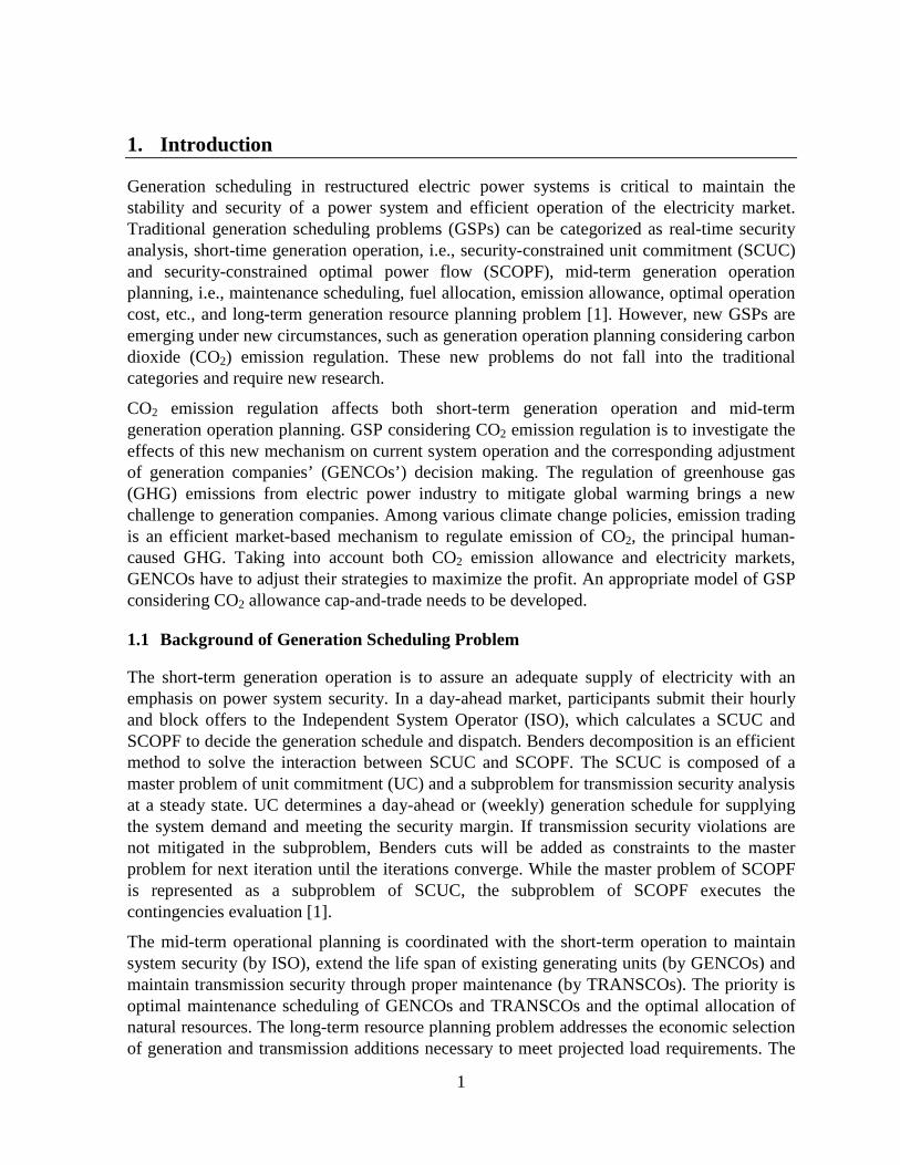
1

1. Introduction

Generation scheduling in restructured electric power systems is critical to maintain the stability and security of a power system and efficient operation of the electricity market. Traditional generation scheduling problems (GSPs) can be categorized as real-time security analysis, short-time generation operation, i.e., security-constrained unit commitment (SCUC) and security-constrained optimal power flow (SCOPF), mid-term generation operation planning, i.e., maintenance scheduling, fuel allocation, emission allowance, optimal operation cost, etc., and long-term generation resource planning problem [1]. However, new GSPs are emerging under new circumstances, such as generation operation planning considering carbon dioxide (CO2) emission regulation. These new problems do not fall into the traditional categories and require new research.

CO2 emission regulation affects both short-term generation operation and mid-term generation operation planning. GSP considering CO2 emission regulation is to investigate the effects of this new mechanism on current system operation and the corresponding adjustment of generation companies’ (GENCOs’) decision making. The regulation of greenhouse gas (GHG) emissions from electric power industry to mitigate global warming brings a new challenge to generation companies. Among various climate change policies, emission trading is an efficient market-based mechanism to regulate emission of CO2, the principal human-caused GHG. Taking into account both CO2 emission allowance and electricity markets, GENCOs have to adjust their strategies to maximize the profit. An appropriate model of GSP considering CO2 allowance cap-and-trade needs to be developed.

1.1 Background of Generation Scheduling Problem

The short-term generation operation is to assure an adequate supply of electricity with an emphasis on power system security. In a day-ahead market, participants submit their hourly and block offers to the Independent System Operator (ISO), which calculates a SCUC and SCOPF to decide the generation schedule and dispatch. Benders decomposition is an efficient method to solve the interaction between SCUC and SCOPF. The SCUC is composed of a master problem of unit commitment (UC) and a subproblem for transmission security analysis at a steady state. UC determines a day-ahead or (weekly) generation schedule for supplying the system demand and meeting the security margin. If transmission security violations are not mitigated in the subproblem, Benders cuts will be added as constraints to the master problem for next iteration until the iterations converge. While the master problem of SCOPF is represented as a subproblem of SCUC, the subproblem of SCOPF executes the contingencies evaluation [1].

The mid-term operational planning is coordinated with the short-term operation to maintain system security (by ISO), extend the life span of existing generating units (by GENCOs) and maintain transmission security through proper maintenance (by TRANSCOs). The priority is optimal maintenance scheduling of GENCOs and TRANSCOs and the optimal allocation of natural resources. The long-term resource planning problem addresses the economic selection of generation and transmission additions necessary to meet projected load requirements. The

2

tradeoff between economics and security is a major consideration in the restructured power system planning. All these GSPs are combinatorial optimization problems with a large number of binary, continuous or discrete decision variables, and various equality and inequality constraints.

Mathematically, GSPs can be formulated as optimization problems with different objective functions and constraints, which are nonconvex, nonlinear, large-scale, mixed-integer combinatorial optimization problems. In the literature, a number of methods, such as enumeration, dynamic programming (DP), Lagrangian Relaxation (LR), Mixed-Integer Programming (MIP), and heuristic methods (genetic algorithms, artificial neural networks, expert and fuzzy systems), have been proposed to achieve an optimal or near optimal solution. However, the high computational burden and high dimensionality are barriers to practical applications.

MIP is a powerful optimization technique to solve combinatorial optimization problems. The optimization problem can be formulated in the MIP format and an optimal solution can be obtained without involving heuristics, which could facilitate the application of MIP approach to large-scale power systems. Although the large number of binary variables could bring a heavy computational burden, the advanced optimization technique of branch-and-cut, which combines branch-and-bound and cutting plane methods, makes MIP method more attractive and applicable together with the commercial software, such as CPLEX, LINDO, etc.

1.2 Greenhouse Gas Emission

GHGs are gases that permit sunlight to go through the earth’s atmosphere and absorb infrared radiation or heat which is re-radiated back to the space but trapped in the atmosphere. GHGs include water vapor, carbon dioxide (CO2), methane (CH4), nitrous oxide (N2O) and ozone (O3). In 2008, total U.S. GHG emissions were 7,052.6 million metric tons carbon dioxide equivalent (MMTCO2e). From 1990 to 2008, total U.S. emissions have risen by 14 percent [2].

The primary GHG emitted by human activities in the U.S. was CO2, representing approximately 81.3 percent of total GHG emissions [2]. The five major fuel consuming sectors contributing to CO2 emissions from fossil fuel combustion are electric power generation, transportation, industrial, residential, and commercial. Electric power generators consumed 37 percent of U.S. energy from fossil fuels and emitted 42 percent of the CO2 from fossil fuel combustion in 2008 [3].

Electricity generators consume 93 percent of total used coal for over half of their required energy in the U.S. in 2008. The type of fuel combusted by electric power generators has a significant effect on their emissions. Therefore, electricity demand significantly impacts coal consumption and CO2 emissions. The total electricity consumption will grow from 4,119 million MWh in 2008 to 5,021 million MWh in 2035, with a 1.0 percent average annual increase [4]. The challenge to the electric power industry is to meet the nation’s energy needs while keeping the emissions from electric power plants within allowable levels.

3

1.3 Emission Regulation Policies

There are various climate change policies to regulate GHG emissions from the electric power industry. The Kyoto Protocol is an international agreement to reduce CO2 and other GHG emissions in an effort to reduce climate change. It required that all industrialized countries reduce the average annual emissions at least 5 percent below the 1990 levels during the 2008 to 2012 period. The Kyoto Protocol also introduced three market-based mechanisms: emission trading, the clean development mechanism and joint implementation [5].

European Union (EU) is committed to cutting its emissions at least 20% below 1990 levels by 2020 [6]. Also, the EU Greenhouse Gas Emission Trading Scheme (ETS) is developed to offer the most cost-effective way for EU members to meet their Kyoto obligations and transform toward a low-carbon economy. ETS allows EU to achieve its Kyoto target at a cost between EUR 2.9 billion and EUR 3.7 billion a year, rather than EUR 6.8 billion a year without ETS. ETS creates incentives to develop technologies for emission reduction [6].

In the U.S., the Regional Greenhouse Gas Initiative (RGGI) is an agreement among the Governors of ten Northeastern and Mid-Atlantic states to reduce GHG emissions from power plants. RGGI operates the first mandatory cap-and-trade program to cap regional power plants’ CO2 emissions, and the cap will be 10 percent lower by 2018 than at the start of the RGGI program in 2009. The initial regional emissions budget is approximately 188 million short tons of CO2, and each allowance to cover one ton of CO2 [7]. State control the number of issued allowances to ensure that total emissions in the region will not exceed the cap. The initial auction will offer allowances through a single-round, uniform-price, sealed-bid auction. RGGI allows market forces to determine the most efficient and cost-effective means to regulate emissions. It is expected to provide a market signal that the cost of emitting carbon must be incorporated into energy pricing.

In response to the Assembly Bill AB32 and Senate Bill 1368, the California Energy Commission (CEC) introduced the “GHG emissions performance standard”. This standard prohibits investor-owned utilities (and later municipal utilities) from entering into long-term contracts to purchase electricity from sources that emit more CO2 than a combined-cycle natural gas plant. While other states have not restricted on emissions from electricity production, six western states and two Canadian provinces have recently announced that they will collaborate in achieving California’s stated goal of reducing 15% of the 2005 GHG emissions by 2020.

1.4 Emission Regulation Methods and Technologies

Carbon capture and storage (CCS) is a method to mitigate climate change by capturing CO2 emissions from large power plants and other sources and storing it instead of releasing it into the atmosphere. However, the capturing process is costly and energy intensive, and CCS technologies are not economically feasible at the present time. Shifting from high CO2 emission power sources to non-CO2 or low CO2 emission power sources, for example, hydroelectric, nuclear, wind, solar, photovoltaic, geothermal, ocean, etc., is an effective method to reduce CO2 emissions. However, all these alternative resources have their limitations. The available and economical hydro resources are being exhausted. The long-term

4

construction period of nuclear power does not help to achieve short-term CO2 emission reduction requirements. Other renewable energy resources have significant potential, but wide applications are limited currently due to either economic infeasibility or lack of maturity in technology.

There have been various research projects about the effects of emission constraints on the electric power system. Reference [9] included emission constraints in classical economic dispatch (ED) by weights estimation technique to solve environmentally constrained economic dispatch (ECED) problem. The work of [10] provided a set of dispatching algorithms to solve the constrained emission dispatch problem with SO2 and NOx emission constraints. References [11-12] presented a short-term unit commitment approach based on Lagrangian Relaxation technique to solve the emission constrained unit commitment (ECUC) problem. However, all these models are developed to solve SO2 or NOx emission regulation problem and these models do provide insights to the CO2 emission regulation without detailed modeling of a CO2 allowance market. References [13-14] formulated the electrical power and NOx allowances market as compementarity problems by using Cournot game. In [15], a nonlinear complementarity model is used to investigate long-run equilibria of alternative CO2 emissions allowance allocation systems in electric power market. However, the daily electricity market and quarterly CO2 allowance auction market should be incorporated in an appropriate time framework.

1.5 Market Equilibrium Model

As the electric power industry becomes market driven, the development of power market provides an opportunity for GENCOs and other market participants to exercise least-cost or profit-based operations. The equilibrium model of generator competition can be used to study the ability of a GENCO to unilaterally exercise market power. Most models use a general method to define a market equilibrium as a set of prices, producer input and output decisions, transmission flows, and consumption that satisfy each market participant’s first-order conditions for maximization of net benefits, i.e., Karush-Kuhn-Tucker (KKT) conditions, while clearing the market [16]. The complete set of KKT and market clearing conditions defines a mixed complementarity problem (MCP). If a market solution exists that satisfies the optimality conditions for each market player along with the market clearing conditions, it will have the property that no participant would alter their decision unilaterally (as in a Nash equilibrium).

There are several types of strategic interactions; they differ in how each generating firm f anticipates how rivals will react to its decisions concerning either prices p or quantities q.

• Pure Competition (No Market Power)/Bertrand: Only qf is the decision variable and p is fixed.

• Generalized Bertrand Strategy (“Game in Prices”): firm f acts as if its rivals’ prices, p* -f, will not change in reaction to changes in f’s prices.

• Cournot Strategy (“Game in Quantities”): firm f acts as if its rivals’ quantities, q*

-f, will not change in reaction to changes in f’s quantities.

5

• Collusion: If f colludes with another supplier, then they would maximize their joint profit.

• Strackelberg: It defines a “leader” whose decisions correctly take into account the reactions of “followers,” who do not recognize how their reactions affect the leader’s decisions.

• General Conjectural Variations (CVs): Output from firms other than f, q-f(qf), is assumed to be a function of qf.

• Conjectured Supply Function (CSF): Output by rivals is anticipated to respond to price according to function q-f(p).

• Supply Function Equilibria (SFE): The decision variables for each firm f are the parameters φf of its bid function qf(p| φf).

In the proposed research, the Cournot model is used with bidding on quantities to analyze the CO2 emission allowance market.

The equilibrium of Nash games is defined as Nash Equilibrium:

Definition: Let f fX ∈X be strategies under the control of firm f; fX the space of feasible

strategies for f; { },f gX X g f−

= ∀ ≠ ; and ( ),f f fX X∗−∏ the payoff to f given the decisions of

all firms. Then, { },fX f∗ ∀ is a Nash Equilibrium in X if

( ) ( ), , ,f f f f f f f fX X X X X f∗ ∗ ∗− −∏ ≥ ∏ ∀ ∈ ∀X .

For Cournot games, f fX q=

2. CO2 Emission Allowance Cap

The CO2 emission allowance capmodel based on the market rules in RGGI. In RGGI, the primary market offer initial allowances through a single-round, uniformbidders is equal to the highest rejected bid. The characteristics of allowance banking, auction limit, CO2 reserve price, offset limit, etc. are considered in the developed model. The model is formulated as an equilibrium problem with equilibrium constraiformulation is transformed inprogramming problem (NLP), which can be solved b

2.1 Bid and Auction

Each GENCO submits its bidding offer

bidding price and iq is the bidding amount.

offers is shown in Figure 1. After market clearance, the COallowance dispatchiA is achieved, as shown in

Figure

6

Emission Allowance Cap-And-Trade Market

emission allowance cap-and-trade market is formulated as the Cournot equilibrium model based on the market rules in RGGI. In RGGI, the primary market offer initial

round, uniform-price, sealed-bid auction. The price paid by allbidders is equal to the highest rejected bid. The characteristics of allowance banking, auction

reserve price, offset limit, etc. are considered in the developed model. The model is formulated as an equilibrium problem with equilibrium constraints (EPEC), and the EPEC

into a nonlinear complemetarity problem (NCP) and nonlinear programming problem (NLP), which can be solved by AMPL/MINOS commercial solver.

its bidding offer( ),i iqλ to the CO2 allowance market,

is the bidding amount. A simple example with three GENCOs’ bidding

. After market clearance, the CO2 allowance priceis achieved, as shown in Figure 2.

Figure 1 GENCOs’ Bidding Offers

Figure 2 Market Clearance

trade market is formulated as the Cournot equilibrium model based on the market rules in RGGI. In RGGI, the primary market offer initial

he price paid by all bidders is equal to the highest rejected bid. The characteristics of allowance banking, auction

reserve price, offset limit, etc. are considered in the developed model. The model is nts (EPEC), and the EPEC

to a nonlinear complemetarity problem (NCP) and nonlinear y AMPL/MINOS commercial solver.

allowance market, where iλ is the

three GENCOs’ bidding

allowance price 2COλ ∗

and the

7

2.2 Problem Formulation

Each GENCO solves the following optimization problem to decide its bidding strategy:

2

2 2

, , , ,

max

max ( )

. . 0

0.033

0

COi i i i

e COi i i i i i i i

P q OS A

i i i i

i i

i i

P a P b P A h OS

s t k P A OS

OS A

P P

λλ λ ∗

∗⋅ − ⋅ + ⋅ − ⋅ − ⋅

≤ ⋅ ≤ +≤ ⋅

≤ ≤

(1)

where eλ is the forecasted electricity price, P is generation output, &a bare coefficients of generator’s cost function, h is the cost rate of offsets, OS is the offset, k is the CO2 emission rate, and maxP is the generation capacity.

Cournot competition models an industry structure in which companies compete on the amount they produce that they decide independently and at the same time. Each GENCO has the bidding price of CO2 allowance to its own expectation. Therefore, in the developed model, the bidding price is the parameter and the bidding amount is the decision variable.

The objective is to maximize the profit, which is the revenue from selling power to electricity market minus the cost of generation, buying allowances from CO2 market and using offsets. The first constraint requires each GENCO to have enough allowances to cover its generated CO2. The second constraint requires that the use of CO2 offset allowances is constrained to 3.3% of a unit’s total compliance obligation during a control period. (Offsets referred to the project-based emissions reductions outside the capped sector.)

The market clearing price is obtained by solving the following optimization problem:

1

2

1

2

max

. .

0.25

0

i

n

j jA

j

nCO

jj

COj

j j

A

s t A CAP

A CAP

A q

λ=

=

⋅

=

≤ ⋅

≤ ≤

∑∑ (2)

where, 2COCAP is the total amount of allowances in the auction.

The first constraint is based on the assumption that all allowances will be sold to assure there is one CO2 allowance price. The second constraint is based on the auction rules in RGGI that it establishes a total limit for the number of allowances that entities may purchase in a single auction, equivalent to 25% of the allowance offered for sale in any single auction. The third constraint restricts that each GENCO’s bought allowances should not exceed its bidding allowances and should be nonnegative.

8

2.2.1 EPEC Model

Given ( ), 1, ,j jq j nλ = K , the optimal solution ( )2, 1, ,COjA j nλ ∗

= K of the concave

optimization problem (2) can be obtained by solving its KKT conditions as follows:

2

1

2 1 2

1

2

3 2

0

0 0

0 01,

0 0

0 0.25 0

nCO

jj

COj j j j

j j j

j j

COj j

A CAP

A w w

w q Aj n

w A

w CAP A

λ λ ∗

=

− =≤ ⊥ − + + − ≥ ≤ ⊥ − ≥ =≤ ⊥ ≥ ≤ ⊥ ⋅ − ≥

∑

K

(3)

KKT conditions (3) are added to each GENCO’s maximization problem (1), and each GENCO’s optimization problem is formulated as the following mathematical problem with equilibrium constraints (MPEC):

2

1 2 3

2 2

, , , ,, , ,

max

2

1

2 1 2

1

2

3 2

max ( )

. . 0

0.033

0

0

0 0

0 0

0 0

0 0.25 0

COi i i

i i i i

e COi i i i i i i i

P q OSA w w w

i i i i

i i

i i

nCO

jj

COj j j j

j j j

j j

COj j

P a P b P A h OS

s t k P A OS

OS A

P P

A CAP

A w w

w q A

w A

w CAP A

λλ λ

λ λ

∗

∗

∗

=

⋅ − ⋅ + ⋅ − ⋅ − ⋅

≤ ⋅ ≤ +≤ ⋅

≤ ≤− =

≤ ⊥ − + + − ≥ ≤ ⊥ − ≥ ≤ ⊥ ≥≤ ⊥ ⋅ − ≥

∑

1,j n=

K

(4)

Each GENCO solves the above MPEC problem and all GENCOs together may reach an equilibrium point of this EPEC.

2.2.2 NCP&NLP Formulation

In the literature, several methods are available to solve the EPEC problem:

1) Diagonalization techniques such as Gauss-Jacobi and Gauss-Seidel type methods. Such methods solve a cyclic sequence of MPEC until the decision variables of all participants reach a fixed point.

2) Sequential nonlinear complementarity problem (SNCP) approach. The approach is related to the relaxation approach used in MPEC that relaxes the

9

complementarity condition of each player and drives the relaxation parameter to zero.

3) Deriving a NCP formulation of the EPEC based on the equivalence between the KKT conditions of the MPEC and strong stationarity. Then EPEC will be solved by standard NCP solvers to MPEC.

The traditional way in the third method is to replace the complementarity condition, such as0 0y s≤ ⊥ ≥ , by 0, 0, 0Ty s y s≥ ≥ ⋅ = , and this equivalent NLP can be solved by using standard NLP solvers. Unfortunately, this NLP violated the Mangasarian-Fromovitz constraints qualification (MFCQ) at any feasible point [17]. Instead, it is proposed to use the method of [18]. Based on that, strong stationarity is equivalent to the KKT conditions of the equivalent NLP.

First, define:

( )( )

( )

2

2 1

2 1 22

2

max

, ,

,

0

0.25 0, 0.033

nCOi i i i

je j

i i i i i i i iCO

CO j j ji i i

j j ji i i i

ji

COji i i i i

i i

i

x P q OS A CAPf x y P a P b P

w wA h OS

H q Ak P A OS

Ak PCAP Ag x y OS A

P P

P

λλ λλ

∗

∗

=

= − = ⋅ − ⋅ − ⋅ − + + −− ⋅ − ⋅ = − ⋅ − − ≥− ⋅ ⋅ − ≥ = − ⋅ − −

∑

( )2 1 2 3, , , ,COj j j j jy A w w wλ ∗

=

(5)

Then the MPEC problem (4) is rewritten in the following compact format:

( )( )

0, ,max ,

. . , 0

01,

0 0

ii

x y s

i

j j

j j

f x y

s t g x y

H sj n

y s

≥

≤− = =≤ ⊥ ≥

K

(6)

where, s is the introduced slack variable.

The NCP formulation is derived by introducing new multipliers:

10

( ) ( ) ( )( ) ( ) ( )

( )( )

, , , 0

, , , 0

0

0 , 0

, 0

0 0

0 0

0 0

0 0

i i ix i x i i x i i i

y i y i i y i i i i

i i i

i i

i i

i i

i i

i

i i i

f x y g x y h x y

f x y g x y h x y s

y

g x y

h x y s

x

s y

y s

µ ξ χµ ξ η

ξ σ ξµ

χψσψ σ η

∇ +∇ +∇ − =

∇ +∇ +∇ + =− + =≤ ⊥ ≥

− =≤ ⊥ ≥≤ + ⊥ ≥≤ + ⊥ ≥≤ + ⊥ ≥

(7)

Definition [18]: A solution of problem (6) is called an equilibrium point of the EPEC. A

solution ( ), , , , , , , ,x y s χ µ ξ ψ σ η∗ ∗ ∗ ∗ ∗ ∗ ∗ ∗ ∗ of (7) is called a strongly stationary point of the

EPEC.

Proposition [18]: If ( ), ,x y s∗ ∗ ∗ is an equilibrium of the EPEC and if every MPEC of (6)

satisfies an MPEC linear independence constraints qualification (MPEC-LICQ), then

there exist multipliers ( ), , , , ,χ µ ξ ψ σ η∗ ∗ ∗ ∗ ∗ ∗ such that (7) hold.

Moreover, to utilize the standard NCP solvers, two alternative formulations will be adopted. The first one is to force the EPEC to identify the basic or minimal multiplier for each player by minimizing the 1l –norm of the multiplier on the complementarity

constraint, as shown in (8).

( ) ( ) ( )( ) ( ) ( )

( )( )

, , , , , , ,1

max

. . , , , 0

, , , 0

0

0 , 0

, 0

0 0

0 0

0 0

0 0

0

i i i

nT

ix y s

i

x i x i i x i i i

y i y i i y i i i i i

i i i

i i

i i

i i

i

i

i

e

s t f x y g x y h x y

f x y g x y h x y s

y

g x y

h x y s

x

y

s

y s

µ ξ ψ σ ηη

µ ξ χµ ξ ψ η

ξ σ ξµ

χψσ

η

=

∇ +∇ +∇ − =

∇ +∇ +∇ − + =− + =≤ ⊥ ≥

− =≤ ⊥ ≥≤ ⊥ ≥≤ ⊥ ≥≤ ⊥ ≥≥

∑

(8)

The second one penalizes the complementarity constraints and results in a well-behaved nonlinear optimization problem by introducing new slack variablesit , as shown in (9).

11

( )( ) ( ) ( )( ) ( ) ( )

( )( )

, , , , , , ,1

min :

. . , , , 0

, , , 0

0

,

,

0, 0

0, 0, 0, 0, 0

0, 0

i i i

nT T T T T

pen i i i i i ix y s

i

x i x i i x i i i

y i y i i y i i i i i

i i i

i i

i i

i i i i i

i i

C x t y s y s

s t f x y g x y h x y

f x y g x y h x y s

y

g x y t

h x y s

y s

x t

µ ξ ψ σ ηχ µ ψ σ

µ ξ χµ ξ ψ η

ξ σ ξ

χ µ ψ σ η

=

= + + + +

∇ +∇ +∇ − =

∇ +∇ +∇ − + =− + =

==

≥ ≥≥ ≥ ≥ ≥ ≥≥ ≥

∑

(9)

Theorem[18]: If ( ), , , , , , , , ,x y s t χ µ ξ ψ σ η∗ ∗ ∗ ∗ ∗ ∗ ∗ ∗ ∗ ∗ is a local solution of (8) with Cpen=0,

then it follows that ( ), ,x y s∗ ∗ ∗ is a strongly stationary point of (4). If

( ), , , , , , , , ,x y s t χ µ ξ ψ σ η∗ ∗ ∗ ∗ ∗ ∗ ∗ ∗ ∗ ∗ is a local solution of (8) with Cpen=0, then it follows

that ( ), ,x y s∗ ∗ ∗ is a strongly stationary point of (4).

Two-GENCO and multi-GENCO case studies are performed with the sensitivity analysis of GENCOs’ bidding prices, electricity price and total amount of CO2 allowances to CO2 allowance price and dispatch. The simulation results demonstrate the joint effect of electricity market and CO2 allowance market, which require an appropriate model for further investigation. The next section is proposed to design the model of generation scheduling problem in both markets.

2.3 Case Study

2.3.1 Two-GENCO Case Study

It is assumed that there are two GENCOs participating in the CO2 allowance auction. The illustrative parameters are shown in Table 1.

Table 1 GENCOs’ Characteristics

GENCO a b λe

($/MW) Pmax

(MW)

Bidding Price

($/p.u.)

k (ton/MW)

h ($/p.u.)

1 15 0.005 20 500 2 1 10

2 18 0.004 20 800 1.5 1 10

In the base case, the reserved bidding prices are assumed to be $2 and $1.5 for GENCO 1 and 2, respectively (given the CO2 allowance price in RGGI now is about $3). Also, the

12

market has a reserved price for CO2 allowance, which is set to be $1 in this simulation. The total allowance number is set to be 700 units. The equilibrium solutions are shown in Table 2.

Table 2 Equilibrium Solutions

GENCO P(MW) A (p.u.) q (p.u.) λCO2 ($/p.u.)

1 350 350 350 1

2 250 350 350

From the result, it is shown that two GENCOs get the same amount of allowances, and they have different reserved bidding prices but same bidding amounts of allowances. GENCO 2 does not use its entire bought allowances and it is able to bank some allowances for future use.

The above is the base case, and it proves that the model is able to reach an equilibrium point of CO2 allowance price and each participant’s bought allowances. The following is the result of a sensitivity analysis of bidding price, forecasted electricity price and total amount of allowances to the CO2 allowance price and allowance distribution level:

• Sensitivity analysis of GENCOs’ bidding price to CO2 allowance price

Both GENCOs’ bidding prices are changed in discrete values from $1 to $3. The result shows that CO2 allowance is always $1 and two GENCOs get the same amount of allowances. This is due to the fact that there are only two players in this Cournot competition. However, this is not a general conclusion, and the result is different in the multi-GENCO case.

• Sensitivity analysis of forecasted electricity price to CO2 allowance price

Table 3 Sensitivity Analysis of Forecasted Electricity Price to CO2 Allowance Price

GENCO λe ($/MW) P(MW) A (p.u.) q (p.u.) Profit of Gen. 1($)

λCO2 ($/p.u.)

1 16 100 300 300 150 1

2 20 250 400 400

1 18 300 300 300 787.5 1

2 20 250 400 400

1 22 420 420 420 1428 1.5

2 20 250 280 392

GENCO 2’s forecasted electricity price is fixed and GENCO 1’s forecasted electricity price changes. If GENCO 1 forecasts a lower electricity price, it will bid less amount of

13

allowance, but get same amount of allowance while banking some allowances. If GENCO 1 forecasts a higher electricity price, it will bid more allowances and get more. Since the electricity price is high, it will use all the allowances to maximize its profit. Also, the CO2 allowance price is higher. Therefore, it is important for GENCOs to correctly forecast the electricity price to participate in the CO2 allowance market.

• Sensitivity analysis of total amount of CO2 allowances to CO2 allowance price

When the allowance is insufficient, GENCO 1 always gets more allowances and CO2 allowance price is higher. It is because GENCO 1 has a higher bidding price. When the allowance is superfluous, some allowances will be banked (it is assumed that all allowance will be sold; otherwise, the clearing price will be zero).

Table 4 Sensitivity Analysis of Total Amount of CO2 Allowances to CO2 Allowance Price

GENCO Total

Allowance P(MW) A (p.u.) q (p.u.)

Profit of Gen. 1($)

λCO2 ($/p.u.)

1 500

300 300 300 600 1.5

2 200 200 300

1 600

350 350 350 613 1.5

2 250 250 350

1 800

400 400 400 800 1

2 250 400 400

2.3.2 Multiple-GENCO Case Study

Four GENCOs participate in the CO2 allowance auction and the total amount of allowances is 1500 units. Their parameters are shown in Table 5.

Table 5 GENCOs’ Characteristics

GENCO a b λe

($/MW) Pmax

(MW)

Bidding Price λ ($/p.u.)

k (ton/MW)

h ($/p.u.)

1 15 0.005 20 500 2 1 10

2 18 0.004 20 800 1.5 1 10

3 10 0.005 20 800 2.5 1 10

4 15 0.004 20 800 2.3 1 10

The equilibrium points are shown in Table 6.

14


GENCO P(MW) A (p.u.) q (p.u.) Profit ($) λCO2 ($/p.u.)

1 262.5 262.5 262.5 574.2

1.5 2 0 0 594 0

3 800 800 800 3600

4 437.5 437.5 437.5 765.6

The results show that GENCO 3 with highest bidding price gets most allowances (each player cannot buy more than 60% of total allowances), while GENCO 2 with the lowest bidding price does not get any allowance.

The market clearing price is set by GENCO 2. If GENCO 2’s reserved price increases but does not exceed $1.9 (the second lowest bidding price), the market clearing price is still set by GENCO2 (results shown in the following table). It proves that this model is capable of finding the equilibrium points of the Cournot competition.


GENCO P(MW) A (p.u.) q (p.u.) Profit ($) λCO2 ($/p.u.)

1 310 310 310 480.5

1.9 2 2.5 2.5 313.3 0.225

3 800 800 800 3280

4 387.5 387.5 387.5 600.625

The above are the simulation results of the NLP formulation of the EPEC model of CO2 allowance cap-and-trade market. It is shown that the model is capable of finding the equilibrium point. When the number of participants in the auction increases, it will become a large-scale optimization problem.

3. Generation Scheduling Problem Considering COMarket

GENCOs participate in the electricity market daily and they aemission allowance market quarterly. They need to know the amount and price of COallowances to make decisions about how to bid in the electricity market, while they bid to CO2 allowance market based on the information of electricitgeneration commitment and dispatch, as shown in

Figure 3 GENCOs’ Interactions in Electricit

Figure

15

Generation Scheduling Problem Considering CO2 Allowance

GENCOs participate in the electricity market daily and they also auction in emission allowance market quarterly. They need to know the amount and price of COallowances to make decisions about how to bid in the electricity market, while they bid to

allowance market based on the information of electricity price and scheduled generation commitment and dispatch, as shown in Figure 3.

GENCOs’ Interactions in Electricity Market and CO2 Allowance Market

Figure 4 Time Horizon of Three-Year GSP

Allowance

lso auction in the CO2 emission allowance market quarterly. They need to know the amount and price of CO2 allowances to make decisions about how to bid in the electricity market, while they bid to

y price and scheduled

Allowance Market

16

Moreover, during the three-year CO2 allowance compliance period, the coordination of midterm generation maintenance scheduling with short-term unit commitment has to be considered to maintain the adequacy in midterm planning and security in short-term operation planning [19-20]. Therefore, in this three-year time framework, generation scheduling problem involving generation maintenance scheduling, unit commitment and CO2 allowance cap-and-trade need to be investigated. The time horizon of three-year GSP is shown in Figure 4.

3.1 MIBLP Formulation

GENCOs’ decision making will be based on the following optimization problem:

Max Total Profit during Time Period T

subject to

Generation Maintenance Scheduling Constraints

SCUC and SCOPF Constraints

CO2 Allowance Cap-and-Trade Market Constraints

Objective function: GENCO’s profit equals to its revenue from selling power to the electricity market minus its cost of maintenance, fuel production, startup, shutdown and CO2 allowance. GENCO maximizes its profit by solving the following problem:

( ){ } { }{ }

{ }

( )

2

, , ,

1

1 1 1

max

. . , ,

1, ,

1 ,

, ,

,

d d d d d d w q q q

d w q q d w qit it it it

d d w

w d

w

w

w w wi

w w

E P SU SD M CO OSiit it it it it it it t it itg x q OS

t t t

d w

it it it

d w

it it

iitt

w

it it it T

it ti

p g C g C C C p A C OS

s t u u x i t t

x u i t t

x T i

x x x i t

x NM t

−

− + −

× − − − − − × + ×

− ≤ ∀ ∈

+ ≤ ∀ ∈

= ∀

− ≤ ∀

≤ ∀

∑ ∑ ∑

∑

∑{ }

( ) { }( ) { }

2

,

2

,

, hydroelectric

1 , ,

1 , ,

,

0.033 ,

, , , 0

d d d

d d

w d

d w

d q q q

d q

q d

d q

d w q q

w

it it itt t

MIN d wi it it

MAX d wiit it

CO IA qi it it it it

i t t

CO qiit it

i t t

it it it it

g g HE i

G x g i t t

g G x i t t

R g A OS A t

OS R g t

g x q OS

∈

∈

≤ × ∀ ∈

× − ≤ ∀ ∈

≤ × − ∀ ∈

× ≤ + + ∀

≤ × × ∀

∀ ≥

∑ ∑

∑∑ (10)

17

Where

( )

( )

( )

11

1

2

, 1,

1

, ,

0, ,

, ,

0, ,

d d d d

w w w

d d d

d

d d d

d

w w w w d

d w

Pi i iit it it it i

M

it it it

kSU d

iit it itj

SU d

it

SD diit it it

SD d

it

IA IA COii t it it it it

i t t

C g a u b g c g

C MT x

C SU u u i t

C i t

C SD u u i t

C i t

A A A OS R g

−=

−

+∈

= × + × + ×= × −

= × − ∀ ≥ ∀ = × − ∀ ≥ ∀

= + + − ×

∑

∑

( )2

2

1

1

1 1

1

1

, ,

, ,

, ,

, , ,

, ,

0, , , 1, ,

d

d d

d d

d d

d d d

d d

d

t

MIN MINi i i i i

kj j d

it itj

kMIN j diit it

j

MIN diit it

j j j d

it it it

k MAX k diit it

j d

it

a b G c G

s i t

g G i t

g G i t

g g i t j

G g i t

i t j k

δ

δ

δδδ

δ

=

=

−

−

= + × + × + × ∀ = + ∀ ≤ − ∀ ≤ − ∀ ≤ − ∀ ≥ ∀ =

∑∑

K

Constraints: Constraints in each subproblem are listed as follows:

1) Generation Maintenance Subproblem: GENCOs are independently responsible for generation maintenance, and they submit the maintenance schedule to ISO, which coordinates with market participants to improve the security of electricity services and reduce the chance of blackouts. The constraints are:

• Maintenance must be scheduled with maintenance windows between the starting and ending times

• Maintenance must be completed within the maintenance duration

• Seasonal limitations

• Maintenance resources availability

( )

,

,

min

. . ,

w w

dit

d w w

d w

M UE

it itgt

w

it it itii t t

C C UE

s t g UE D t∈

+ ×

+ = ∀

∑∑ ∑ (11)

2) SCUC and SCOPF Subproblem: The short-term (daily/weekly) SCUC problem can be formulated in MILP formulation [20]. The constraints are:

• Power balance

• System spinning and operating reserve requirements

• Generation unit capacity limits

• Ramping rate limits

• Minimum ON/OFF time limits

• Transmission flow limits

18

• Contingency analysis

( ){ }

1

max

. . ,

,

,

, ,

, ,

, ,

, ,

d d d d

d dit

d d

d d

d d

d d

d d d d

d d d

d d d

d d

P SU SD

it it it itgi t

d

it iti i

S S d

it ti

O O d

it ti

MIN di it it

S O MAX diit it it it

S S d

it t it

O O d

it t it

it it

C g C C

s t g D t

r R t

r R t

G u g i t

g r r G u i t

r R u i t

r R u i t

g g MaxI−

+ +

= ∀

≥ ∀

≥ ∀

× ≤ ∀

+ + ≤ × ∀

≤ × ∀

≤ × ∀

− ≤

∑∑∑ ∑∑∑

( ) ( )( ) ( )

( )

1

1 1

1 1

max

, ,

, ,

0, ,

0, ,

, ,

d d

d d d

d d d

d d

di

diit it

ON ON diit it it

OFF OFF diit it it

dki kit it

i

nc i t

g g MaxDec i t

Y T u u i t

Y T u u i t

PTDF g D F i t

−

− −

− −

∀

− ≥ − ∀

− × − ≥ ∀

− × − ≥ ∀

× − ≤ ∀∑ (12)

( )

( ) ( )

2

max

1min

2

. . 0,

,

0

d d

dit

d d d

d d d

d

i iit itgi

it it ti i

k i kit it kti

it

g g

s t g D

GSF g D F k

g

α β

λ

µ−

× + × × − =

× − ≤ ∀∀ ≥

∑∑ ∑∑

(13)

Where

d d d d d d

E energy congk iit it it it t kt

i

p LMP LMP LMP GSFλ µ−

= = + = + ⋅∑

The solutions of SCUC problem will provide the commitment of generation units. Based on this, solving the SCOPF problem hourly will get the generation dispatch and locational marginal price (LMP).

3) CO2 Allowance Cap-and-Trade Market: The CO2 allowance market clearing price is obtained by solving the optimization problem.

19

( )2

2 2

2

max

. . 0,

0.25 , ,

0

, 0

q q

qit

q q q

q q

q q

q q

CO

it itAi

CO q CO

it t ti

CO q

it t

it it

it it

B A

s t A CAP t p

A CAP i t

A q

A q

⋅

− = ∀

≤ ⋅ ∀≤ ≤

∀ ≥

∑∑

(14)

There is a coupling constraint between generation maintenance and unit commitment, i.e., a unit cannot be committed if the unit is on maintenance.

Decision Variables:

ftA ′ Amount of allowances distributed to firm f in interval t’

ftOS ′ Offsets used by firm f in interval t’

2COtp ′ CO2 allowance price in interval t’ [$/p.u.] Eitp LMP at node i in period t [$/MWh]

itg Power output of generator i in period t [MW]

itI Binary variable of the commitment of generation i in period t

itX Binary variable of the maintenance schedule of generation i in

period t

The three-year GSP is formulated as a Mixed Integer Bilevel Linear Programming (MIBLP) problem. The global optimal solutions of continuous variables of CO2 allowance price 2CO

tp ′ , LMP Eitp and generation dispatchitg , binary variables of unit

commitment itI and generation maintenance scheduleitX , and integer variables of

allowance dispatch ftA ′ and offsets usage ftOS ′ are obtained by solving this MIBLP

problem.

3.2 Solution Methodology

Based on [21], the proposed solution methodology is described as follows. The MIBLP problem can be written in a compact format, i.e.,

20

,max 1* 1*

. . 1* 1* 1

arg max 2* 2*

. . 2* 2* 2

0 integer

0 integer

x y

w

I

J

C x d y

s t A x B y b

y C x d w

s t A x B w b

w w

x x

+

+ ≤∈ +

+ ≤≥

≥

(15)

1) Fix the values of the binary variablesz z= , and solve the bilevel linear programming (BILP) problem:

( )( )( )

, ,

,

max 1* 1* 1

. . 1* 1* 1 1

max 2* 2* 2

. . 2* 2* 2 2 1

0 2

0 3

x y z

y z

D x E y F z

s t A x B y b C z

D x E y F z

s t A x B y b C z w

x w

y w

+ + ∗

+ ≤ − ∗+ + ∗

+ ≤ − ∗

− ≤

− ≤

(16)

Where w1, w2, w3 are the dual variables of the constraint.

2) Based on KKT conditions, replace the lower level problem by complementarity constraints and add them to the upper level problem. Then solve the following linear problem with complementarity constraints (LPCC):

,max 1* 1* 1

. . 1* 1* 1 1

0 2 2 2* 2* 1 0

0 2* 2 2 0

0 2* 3 2 0

x yD x E y F z

s t A x B y b C z

b C z A x B y w

A w D x

B w E y

+ + ∗

+ ≤ − ∗≤ − ∗ − − ⊥ ≥≤ − ⊥ ≥≤ − ⊥ ≥

(17)

By using the “θ-free algorithm for LPCC” from reference [22], (17) can be solved.

3) From the solution of (17), it is known which constraint in (15) is active. Then formulate the following linear programming problem by removing the optimality constraint of the lower level problem and set the active constraint (here randomly assume one for illustration purpose) to be the equality:

,max 1* 1* 1

. . 1* 1* 1 1

2* 2* 2 2

, 0

x yD x E y F z

s t A x B y b C z

A x B y b C z

x y

+ + ∗

+ = − ∗+ ≤ − ∗

≥

(18)

4) Introduce slack variables to write (18) in the following compact format:

21

( )max

. . *

0

sH s

s t M s b C z u

s

∗

= − ∗

≥

(19)

The dual of (19) is:

( )min

. .

free

uu b C z

s t u M H

u

∗ − ∗

∗ ≥ (20)

Where, u is the dual variable of constraint in problem (19).

Based on Farkas Lemma, the necessary and sufficient condition for (19) to have at least one non empty solution for z is: Problem (19) has a solution s if and only if

( ) 0u b C z∗ − ∗ ≥ and 0u M∗ ≥ for all u.

When choosing z arbitrarily, there is a finite number of possibilities:1 2, , , nz z zL . For

each zi, there is a corresponding inequality constraint. Then to make sure (5) has at least one nonempty solution, solve the following Master Problem (MP):

( )

( )

( )

( )

( )

( )( )

( )

( )

( )

( )

( )

1 2

1 2

1 2

1 2

1 1 1 2 1

1 2

1 1 1 2 1

1 2

max

. .

0 0 0

0 0 0

n

n

n

n

zz zn

z z zP K R n

zz zn

z z zP K R n

u b C z u b C z u b C z

s t




ξξ ξ ξ

ξ ξ ξ

∗ − ∗ ≥ ∗ − ∗ ≥ ∗ − ∗ ≥ ∗ − ∗ ≥ ∗ − ∗ ≥ ∗ − ∗ ≥ ∗ − ∗ ≥ ∗ − ∗ ≥ ∗ − ∗ ≥ ∗ − ∗ ≥ ∗ − ∗ ≥ ∗ − ∗ ≥

L L L L

L L L L

free, binaryzξ

(21)

Since the values of all zi are obtained during the iteration process, only some constraints in (21) are known explicitly. Then in each step, the problem solved is called a Restricted Master Problem (RMP). The solution of RMP will provide an upper bound of the original problem, and solution of (17), which is called the Slave Problem (SP), will provide a lower bound. It is because RMP is a relaxation of the original problem whereas the SP represents a restriction.

5) Solve (19), and based on the solution to add the cut: i. Feasibility Cut:

If dual of (19) is unbounded, add the constraint to RMP:

( ) 0u b C z∗ − ∗ ≥ (22)

where u is the extreme ray of dual problem (19).

22

ii. Integer Exclusion Cut:

If the optimal solution exists and ( )u b C z ξ∗ − ∗ ≥ , but the difference between upper

and lower bound exceeds the threshold, add the following constraints to RMP:

1i ji P j Q

z z P∈ ∈

− ≤ −∑ ∑ (23)

Where P is the set of z’s value is 1, and Q is the set of z’s value is 0. |P| is the number of variables z that has value of 1. iii. Optimality Cut:

If optimal value of dual (19) is bounded, but ( )u b C z ξ∗ − ∗ < , add the constraint to

RMP:

( )u b C z ξ∗ − ∗ ≥ (24)

3.3 Algorithm

Step 1: Divide the MIBLLP problem into one RMP (21) and several SPs (16) by fixing binary variables. In the initial step, RMP will only have the objective, and constraints are added in future iterations from the cut of solving SP. RMP will provide an upper bound.

Step 2: Transfer SP problem to LPCC problem (problem 17), and solve it by θ-free algorithm. SP is the restricted MIBLLP, and it provides a lower bound. The decomposition technique allows parallel computation of solving multiple SPs.

Step 3: From the solution of LPCC problem, construct the LP problem (problem 18 and 19)

1) If solution is unbounded, add the feasibility cut: ( ) 0u b C z∗ − ∗ ≥ , go to Step 4;

2) If solution is bounded, which provides a lower bound, and restricts RMP

( ( )u b C z ξ∗ − ∗ < ), add the optimality cut (constraint): ( )u b C z ξ∗ − ∗ ≥ , and

go to step 4; 3) If solution is bounded, which provides a lower bound, but does not restrict RMP

( ( )u b C z ξ∗ − ∗ ≥ ), add the Exclusion cut: 1i ji P j Q

z z P∈ ∈

− ≤ −∑ ∑ , and go to step 4.

Step 4: Solve RMP with added cut, and get an updated upper bound. Find the difference between upper bound and lower bound. If it is within the tolerance, stop; otherwise, update the SP by setting constraint of current binary variable z and go back to Step 2.

The flow chart of the proposed algorithm is shown in Figure 5:

Figure

3.4 Case Study

The PJM 5-Bus System is used for illustration of the methodology. It is assumed all five GENCOs participate in GENCO 1 also participates in Cmaintenance scheduling of GENCO 1, daily unit commitment and hourly economic dispatch, and one CO2 allowance market auction with three bidding strategies of GENCO 1 are considered in this case.

3.4.1 System Data

System topology, branch data, generation data, electricity market, maintenance limitgiven as follows.

23

Figure 5 Flow Chart of Algorithm

is used for illustration of the proposed model and solution It is assumed all five GENCOs participate in the electricity market and

GENCO 1 also participates in CO2 allowance market. The seven-week generation maintenance scheduling of GENCO 1, daily unit commitment and hourly economic

allowance market auction with three bidding strategies of GENCO

tem topology, branch data, generation data, load data, GENCOs’ bidding maintenance limit and CO2 bidding offer of GENCO 1

Figure 6 PJM 5-Bus System

proposed model and solution electricity market and

week generation maintenance scheduling of GENCO 1, daily unit commitment and hourly economic

allowance market auction with three bidding strategies of GENCO

GENCOs’ bidding offers in of GENCO 1 have been

24

Table 8 Branch Data

Branch From Bus To Bus Reactance X Limit 1 1 2 0.0281 2.50 2 1 4 0.0304 1.5 3 1 5 0.0064 4 4 2 3 0.0108 3.5 5 3 4 0.0297 2.4 6 4 5 0.0297 2.4

Table 9 Generation Data

Generator Bus Fixed cost

($/hr) Startup cost ($)

Shutdown cost ($)

Ramp up limit

Ramp down limit

1 1 50 100 20 1.2 1.4 2 1 60 150 20 1.2 1.4 3 3 70 200 20 0.8 1 4 4 150 400 20 1 1.2 5 5 50 120 20 1 1.2

Figure 7 1-week Load Data

Table 10 GENCOs’ Electricity Bidding Offers/Production Cost ($/pu-hr)

Generator Block 1 Block 2 Block 3 Price 1 Price 2 Price 3 1 0.2 0.3 0.2 13 14 16 2 0.2 0.3 0.3 12 13 16 3 0.4 1 0.4 15 18 20 4 0.6 1 0.4 16 18 21 5 0.2 0.3 0.2 13 14 16

0

50

100

150

200

250

300

350

400

1 25 49 73 97 121 145

M

Hour

25

Table 11 Maintenance Limit of GENCO 1

Equipment From Bus To Bus Windows Duration

(hrs) Cost ($/hr)

G1 1 / Mon. – Sun. 24 84

Table 12 CO2 Allowance Bidding Offers of GENCO 1

Strategy q (p.u.) λCO2 ($/p.u.)

1 11000 1.60

2 12000 1.62

3 13000 1.65

3.4.2 Simulation Results

The profit and generation output of GENCO 1 utilizing three bidding strategies in CO2 allowance market are shown in Table 13. Each column represents the seven-day maintenance activity during that week.

Table 13 GENCO 1’s Profit and Generation Output under Different Strategies

Maintenance

Schedule Week

1 Week

2 Week

3 Week

4 Week

5 Week

6 Week

7 Base Case

Profit/ 103$ 942.9 968.45 1016.54 989.1 773.92 770.28 1041.18

Generation/

103 MW 51.94 53.41 55.86 54.39 43.61 43.12 56.84

Strategy 1

Profit/ 103$ 754.6 780.15 847.56 800.31 598.22 593.25 826

Generation/

103 MW 48.58 49.96 53.17 50.88 40.79 40.33 52.25

Strategy 2

Profit/ 103$ 805 831.32 880.04 852.6 636.79 633.22 904.82

Generation/

103 MW 51.94 53.41 55.86 54.39 43.61 43.12 56.84

Strategy 3

Profit/ 103$ 791.56 817.88 866.46 839.02 623.35 619.78 891.31

Generation/

103 MW 51.94 53.41 55.86 54.39 43.61 43.12 56.84

The comparison of profit is shown in Figure 8. In the base case, GENCO 1 only participates in the electricity market, and obtains the highest profit. When GENCO 1 participates in both electricity market and CO2 allowance market, it receives less profit and the profits are different using various bidding strategies. Also, seven maintenance schedules result in different profits.

Figure The comparison of generation outputmore generation output as it participates in both markets,

Figure 9 Comparison of Generation Output for Optimal maintenance scheduling and COFigure 10. It is seen that the bidding strategies in CO2 allowance market. Bidding strategy 2 bring

0

200

400

600

800

1000

1200

1

103 $

0

10

20

30

40

50

60

1 2

Generation Output of G1

103 M

W

26

Figure 8 Comparison of Profit for GENCO 1

The comparison of generation outputs is shown in Figure 9. Similarly, GENCO 1 has as it only participates in the electricity market. When GENCO 1

, bidding Strategy 2 always brings most generation output.

Comparison of Generation Output for GENCO 1

Optimal maintenance scheduling and CO2 allowance bidding strategy are shown in the optimal maintenance schedule is different using three

allowance market. Bidding strategy 2 brings the highest profit.

2 3 4 5 6 7

Profit of G1

Base Case

Strategy 1

Strategy 2

Strategy 3

Week

3 4 5 6 7

Generation Output of G1

Base Case

Strategy 1

Strategy 2

Strategy 3

Week

. Similarly, GENCO 1 has city market. When GENCO 1

generation output.

allowance bidding strategy are shown in is different using three

s the highest profit.

Base Case

Strategy 1

Strategy 2

Strategy 3

Base Case

Strategy 1

Strategy 2

Strategy 3

Figure 10 Optimal Maintenance Scheduling & CO The comparison of profits from different COFigure 11. It is shown that Strategy 2 is the best bidding strategy, which means GENCO 1 should not bid too many allowances (Strategy 3) or too few allowances (Strategy 1). The optimal bidding strategy can be obtained by solving the proposed optimization problem.

Figure 11 The Comparison of Profits from Different Strategies

0200400600800

10001200

Base Case (Week 7)

1041.18

Optimal Maintenance Scheduling & CO

103 $

400

500

600

700

800

900

1000

Strategy 1

103

$

Comparison of Profits from Different Strategies

27

Optimal Maintenance Scheduling & CO2 Allowance Bidding Strategy

The comparison of profits from different CO2 allowance bidding strategies is shown in. It is shown that Strategy 2 is the best bidding strategy, which means GENCO 1

bid too many allowances (Strategy 3) or too few allowances (Strategy 1). The g strategy can be obtained by solving the proposed optimization problem.


Base Case (Week 7)

Strategy 1 (Week 2)

Strategy 2 (Week 7)

Strategy 3 (Week 7)

1041.18847.56 904.82 891.31

Optimal Maintenance Scheduling & CO2 Allowance Bidding

Strategy

Strategy 1 Strategy 2 Strategy 3


Allowance Bidding Strategy

allowance bidding strategies is shown in . It is shown that Strategy 2 is the best bidding strategy, which means GENCO 1

bid too many allowances (Strategy 3) or too few allowances (Strategy 1). The g strategy can be obtained by solving the proposed optimization problem.

Strategy 3

891.31

Optimal Maintenance Scheduling

Week 1

Week 2

Week 3

Week 4

Week 5

Week 6

Week 7

28

3.4.3 Conclusions

1. Optimal maintenance scheduling will be changed considering different CO2

allowance bidding strategies. 2. Under three bidding strategies, which correspond to small, medium and large (can

be used in secondary market) amount of allowances, GENCOs will have different profits. Bidding strategy of either small or large amount of allowances cannot make most profit. The optimal bidding strategy is connected with optimal maintenance scheduling.

3. Based on the proposed model, GENCOs will be able to determine their optimal mid-term generation maintenance scheduling and CO2 emission allowance bidding strategy participating in both electricity market and CO2 allowance market.

29

4. Conclusions

In the competitive market environment, GENCOs can schedule the maintenance periods to maximize their own profits, which also consider ISO’s functionality from the view point of system reliability and cost minimization. Carbon mitigation policies, such as CO2 allowance cap-and-trade market, help to reduce consumption in traditional energy and promote to shift to renewable energy resources. Considering these new effects, GENCOs need to adjust their scheduling strategies in the electricity market and bidding strategies in CO2 allowance cap-and-trade market. The proposed research addresses the challenging issue of generation scheduling under new environmental considerations. The emission-constrained generation scheduling problem involving generation maintenance scheduling, unit commitment and CO2 allowance cap-and-trade is investigated.

First, the CO2 emission allowance cap-and-trade market is formulated as the Cournot equilibrium model. Practical market rules, such as those in RGGI, are considered in the developed model. The sensitivity of GENCOs’ bidding price, electricity price and total amount of CO2 allowances to CO2 allowance price and dispatch are analyzed. Then, the model of generation scheduling problem involving generation maintenance scheduling, unit commitment and CO2 allowance cap-and-trade, in the three-year CO2 allowance compliance period, is proposed.

Based on the proposed model, GENCOs are able to know the amount and price of CO2 allowances to make bidding decisions in the electricity market, while they bid to CO2 allowance market based on the information of electricity price and scheduled generation commitment and dispatch. With this information, GENCOs will be able to determine their optimal mid-term operation planning and short-time operation schedules participating in both electricity market and CO2 allowance market. To the best of the authors’ knowledge, this problem has not been solved. A solution to this new problem is proposed in this research.

In the future work, the development of an accurate CO2 emission model related with generation output is critical. The current emission model is to simply multiply generation output by constant emission rate to obtain the emitted CO2. With more insight into the physical mechanisms, a more accurate model will be beneficial. Also, the three-year optimization problem will be solved with weekly generation maintenance scheduling and quarterly CO2 allowance market auctions.

30

References

[1] M. Shahidehpour, W. Tinney, and Y. Fu, “Impact of security on power system operation,” Proceedings of the IEEE, vol. 93, no. 11, pp. 2013- 2025, Nov. 2005.

[2] U.S. Energy Information Administration, “Emissions of greenhouse gases in the United States 2008,” Dec. 2009, URL: http://www.eia.doe.gov/oiaf/1605/ggrpt/pdf/0573(2008).pdf

[3] U.S. Environmental Protection Agency, “Inventory of U.S. greenhouse gas emissions and sinks: 1990 to 2008,” Apr. 2010, URL: http://www.epa.gov/climatechange/emissions/downloads10/US-GHG-Inventory-2010_Report.pdf

[4] U.S. Energy Information Administration, “Table 8. Electricity Supply, Disposition, Prices, and Emissions”, Dec. 2009, URL: http://www.eia.doe.gov/oiaf/aeo/excel/aeotab_8.xls

[5] Kyoto Protocols to the United Nations Framework Convention on Climate Change, “United Nations framework convention on climate change, United Nations,” 1998, URL: http://unfccc.int/resource/docs/convkp/kpeng.pdf.

[6] European Commission, “EU action against climate change: EU emissions trading – an open scheme promoting global innovation,” Sep. 2005, URL: http://ec.europa.eu/environment/climat/pdf/emission_trading2_en.pdf.

[7] Regional Greenhouse Gas Initiative, Inc., “Design elements for regional allowance auctions under the Regional Greenhouse Gas Initiative,” URL:

http://www.rggi.org/docs/20080317auction_design.pdf

[8] Environmental Defense Fund, “Cap and Trade 101”, Mar. 2009, URL: http://www.edf.org/documents/4348_CapAndTradeBasics.pdf

[9] R. Ramanathan, "Emission constrained economic dispatch," IEEE Trans. Power Systems, vol.9, no.4, pp.1994-2000, Nov 1994.

[10] J. W. Lamont and E. V. Obessis, "Emission dispatch models and algorithms for the 1990s," IEEE Trans. Power Systems, vol.10, no.2, pp.941-947, May 1995.

[11] T. Gjengedal, "Emission constrained unit-commitment (ECUC)," IEEE Trans. Energy Conversion, vol.11, no.1, pp.132-138, Mar 1996.

[12] K.H. Abdul-Rahman, S. M. Shahidehpour, M. Aganagic, and S. Mokhtari, “A practical resource scheduling with OPF constraints,” IEEE Trans. Power Systems, vol. 11, no. 1, pp. 254-259, Feb. 1996.

[13] Y. Chen, B.F. Hobbs, S. Leyffer, and T. Munson, "Solution of large-scale leader-follower market equilibria problems: electric power and NOx permit markets," Computational Management Science, vol. 3, no. 4, pp. 307-330, Aug. 2004.

31

[14] Y. Chen and B. F. Hobbs, “An oligopolistic power market model with tradable NOx permits,” IEEE Trans. Power Systems, vol. 20, no. 1, pp. 119-129, Feb. 2005.

[15] J. Z. Schulkin, B. F Hobbs, and J. S. Pang, “Long-run equilibrium modeling of alternative emissions,” Cambridge Working Papers in Economics from Faculty of Economics, University of Cambridge, Sept. 2007.

[16] J. Z. Schulkin, B. F Hobbs, and J. S. Pang, “Long-run equilibrium modeling of alternative emissions,” Cambridge Working Papers in Economics from Faculty of Economics, University of Cambridge, Sept. 2007.

[17] R. Fletcher, S. Leyffer, D. Ralph, and S. Scholtes. “Local convergence of SQP methods for mathematical programs with equilibrium constraints,” Numerical Analysis Report NA/209, Department of Mathematics, University of Dundee, Dundee, UK, May 2002.

[18] S. Leyffer and T. Munson, “Solving multi-leader-follower games,” Argonne National Laboratory, Apr. 2005.

[19] Y. Fu, et al., “Coordination of midterm outage scheduling with short-term security-constrained unit commitment,” IEEE Trans. Power Systems, vol. 24, no. 4, pp. 1818-1830, Nov. 2009.

[20] M. Carrion and J. M. Arroyo, “A computationally efficient mixed-integer linear formulation for the thermal unit commitment problem,” IEEE Trans. Power Systems, vol. 21, no. 3, pp. 1371-1378, Aug. 2006.

[21] G. K. Saharidis, M. G. Ierapetritou, “Resolution method for mixed integer bi-level linear problems based on decomposition technique,” Journal of Global Optimization, Mar. 2008.

[22] Lizhi Wang, “θ-free algorithm for LPCC”, IE 634X Computational Optimization, Iowa State University, Spring 2010.

Documents

Technical and Economic Implications of Greenhouse Gas