Embed Size (px)
Citation preview

Accepted Manuscript
Greenhouse gas assessment of soybean production: implications of land use changeand different cultivation systems
Érica Geraldes Castanheira, Fausto Freire
PII: S0959-6526(13)00344-2
DOI: 10.1016/j.jclepro.2013.05.026
Reference: JCLP 3465
To appear in: Journal of Cleaner Production
Received Date: 13 December 2012
Revised Date: 10 May 2013
Accepted Date: 17 May 2013
Please cite this article as: Castanheira ÉG, Freire F, Greenhouse gas assessment of soybeanproduction: implications of land use change and different cultivation systems, Journal of CleanerProduction (2013), doi: 10.1016/j.jclepro.2013.05.026.
This is a PDF file of an unedited manuscript that has been accepted for publication. As a service toour customers we are providing this early version of the manuscript. The manuscript will undergocopyediting, typesetting, and review of the resulting proof before it is published in its final form. Pleasenote that during the production process errors may be discovered which could affect the content, and alllegal disclaimers that apply to the journal pertain.

MANUSCRIP
T
ACCEPTED
ACCEPTED MANUSCRIPT
Highlights:
• LC GHG balance of soybean is dominated by LUC emissions.
• Significant GHG variation was calculated for LUC scenarios and cultivation
systems.
• Tillage systems have higher GHG emissions than reduced-(no-)tillage systems.
• Uncertainty in N2O is high and dominates cultivation GHG emissions

MANUSCRIP
T
ACCEPTED
ACCEPTED MANUSCRIPT
8905
Greenhouse gas assessment of soybean production:
implications of land use change and different cultivation
systems
Érica Geraldes Castanheiraa and Fausto Freirea,*
aADAI-LAETA, Department of Mechanical Engineering, University of Coimbra, Pólo II
Campus, Rua Luís Reis Santos, 3030-788 Coimbra, Portugal
*Corresponding author. Tel.: +351 23979039; Fax: +351 23979001; E-mail address:
[email protected] (F. Freire)
Abstract
The increase in soybean production as a source of protein and oil is being stimulated
by the growing demand for livestock feed, food and numerous other applications.
Significant greenhouse gas (GHG) emissions can result from land use change due to
the expansion and cultivation of soybean. However, this is complex to assess and the
results can vary widely. The main goal of this article is to investigate the life-cycle GHG
balance for soybean produced in Latin America, assessing the implications of direct
land use change emissions and different cultivation systems. A life-cycle model,
including inventories for soybean produced in three different climate regions, was
developed, addressing land use change, cultivation and transport to Europe. A
comprehensive evaluation of alternative land use change scenarios (conversion of
tropical forest, forest plantations, perennial crop plantations, savannah and
grasslands), cultivation (tillage, reduced tillage and no-tillage) and soybean
transportation systems was undertaken. The main results show the importance of land
use change in soybean GHG emissions, but significant differences were observed for
the alternative scenarios, namely 0.1-17.8 kg CO2eq kg-1 soybean. The original land

MANUSCRIP
T
ACCEPTED
ACCEPTED MANUSCRIPT
choice is a critical issue in ensuring the lowest soybean GHG balance and degraded
grassland should preferably be used for soybean cultivation. The highest GHG
emissions were calculated for tropical moist regions when rainforest is converted into
soybean plantations (tillage system). When land use change is not considered, the
GHG intensity varies from 0.3 to 0.6 kg CO2eq kg-1 soybean. It was calculated that all
tillage systems have higher GHG emissions than the corresponding no-tillage and
reduced tillage systems. The results also show that N2O emissions play a major role in
the GHG emissions from cultivation, although N2O emission calculations are very
sensitive to the parameters and emission factors adopted.
Keywords: Carbon footprint; Carbon stocks; Land conversion; Life Cycle Assessment
(LCA); Soil management; Tillage.
1 Introduction
The increase in soybean production as a source of protein and oil is being stimulated
by the growing demand for livestock feed, food and numerous other applications (e.g.
biodiesel, bioplastics and lubricants). The global production of soybean more than
doubled in the period 1995-2011 to a new record volume of 263.8 million tonnes
(2010/11). The major world soybean producers in 2010/11 were the United States of
America (90.6 million tonnes), Brazil (73.8 million tonnes) and Argentina (49.5 million
tonnes). There was an impressive growth in soybean production in Brazil and
Argentina, mainly associated with an expansion in cultivation areas of 126% and 209%
respectively during the period 1995-2011 (Product Board MVO, 2011).
Important environmental concerns have emerged regarding carbon stock changes due
to the land use changes (LUC) needed for the expansion of the soybean cultivation
area. LUC, together with soybean cultivation, can result in significant greenhouse gas
(GHG) emissions. However, the assessment of soybean GHG intensity is complex and
the results can vary widely due to several factors, namely: i) the uncertainty of soil

MANUSCRIP
T
ACCEPTED
ACCEPTED MANUSCRIPT
emissions (Smeets et al., 2009), in particular nitrous oxide (N2O) and carbon dioxide
(CO2) emissions due to LUC (Kendall and Chang, 2009); ii) the diversity of soil
management practices (e.g. tillage, reduced tillage, no-tillage), material inputs,
locations and yields (Nemeck et al., 2012; Kim and Dale, 2009); and iii) the different
distances and types of soybean transport in question.
The life-cycle (LC) GHG balance of soybean-based products has been assessed in
various publications in recent years, e.g. Alvarenga et al.(2012), Castanheira and
Freire (2012), Mourad and Walter (2011), Prudêncio da Silva et al.(2010), Omni Tech
International (2010), Tsoutsos et al. (2010), Panichelli et al.(2009), Lehuger et al.
(2009), van Dam et al. (2009), Reinhard and Zah (2009), Dalgaard et al. (2008),
Reijnders and Huijbregts (2008), Searchinger and Heimlich(2009), Huo et al.(2008,
2009), Kim and Dale(2009), Miller et al. (2007). However, only some studies accounted
for carbon emissions from direct LUC and a wide range of results was reported (e.g.
Kim and Dale, 2009; Searchinger and Heimlich, 2009; Prudêncio da Silva et al., 2010;
Castanheira and Freire, 2012; van Dam et al., 2009; Panichelli et al., 2009; Reinhard
and Zah, 2009; Reijnders and Huijbregts, 2008; Daalgard et al., 2008). The differences
in the results are mostly related to LUC modeling assumptions, namely: i) the LUC
area, ii) previous land use (e.g. forest, savanna, grassland), iii) the duration of land use
for soybean production (e.g. 10 or 25 years) and iv) LUC location (Ponsioen and Blonk,
2012).The wide range of results shows that producing general figures to quantify direct
LUC in the GHG emissions balance is difficult and each case should be addressed
individually (Börjesson and Tufvesson, 2011; Cherubini, 2010).
The influence of management practices on LC GHG emissions from agricultural
products is a challenging issue (Flysjö et al., 2012; Hokazono and Hayashi, 2012;
Chamberlain et al., 2011; Knudsen et al., 2010; Basset-Mens et al., 2007). A small
number of studies have addressed alternative agricultural systems in order to assess
the effects of different soybean management practices and identify the greatest source
of GHG emissions in each system. In addition, N2O emissions from nitrogen (N)

MANUSCRIP
T
ACCEPTED
ACCEPTED MANUSCRIPT
additions and mineralization of soil organic matter were identified as a major contributor
to the soybean GHG balance (Brandão et al., 2010; Snyder et al., 2009; Reijnders and
Huijbregts, 2008; Landis et al., 2007), since N2O has a high Global Warming Potential
in relation to CO2 (1 kg N2O is equivalent to 298 kg CO2eq, for a 100 year time-
horizon). However, there are significant uncertainties in N2O emission calculations
(IPCC, 2006), particularly for N2O emissions originating in the fraction of N lost via
runoff, leaching and volatilization (Reijnders and Huijbregts, 2011). In addition, only a
few studies have assessed how this influences the soybean GHG balance (Del Grosso
et al., 2009; Smeets et al., 2009; Snyder et al., 2009; Panichelli et al., 2009; Smaling et
al., 2008; Reijnders and Huijbregts, 2008; Miller, 2010; Miller et al., 2006).
The transportation of soybean can represent an important contribution to the GHG
balance (Prudêncio da Silva et al., 2010). Soybean is transported long distances by
road and 42% of the soybean produced in Brazil (and 25% in Argentina) was exported
for processing in other countries (Product Board MVO, 2011). Although long distance
transoceanic transport might increase GHG emissions slightly, Prudêncio da Silva et al.
(2010) showed that the place of origin of soybean within Brazil strongly affects its
environmental impact, due to the current predominance of road transport.
Alternative LUC scenarios, cultivation and transportation systems can be critical in
terms of soybean LC GHG intensity. This has not been addressed comprehensively in
previous research. The main purpose of this article is to present an LC GHG
assessment of soybean produced in Latin America (LA) and exported to the European
Union (EU). A comprehensive evaluation of the implications of 45 scenarios (a
combination of alternative LUC, cultivation systems, soil types and climate regions)
was undertaken. A sensitivity analysis to field N2O emissions was implemented, since
there is significant uncertainty regarding the emission factors and partitioning fractions
(volatilization and leaching factors) adopted in calculations (IPCC, 2006). Default,
maximum and minimum values from the IPCC (2006) for emission factors and
partitioning fractions were adopted to assess the influence on field N2O emission

MANUSCRIP
T
ACCEPTED
ACCEPTED MANUSCRIPT
calculations. An analysis of the effect of soybean origins on GHG intensity was also
implemented for various types of lorry and distances between plantations and ports.
The article is organized in 4 sections, including this introduction. Section 2 presents the
LC model and inventory for soybean, including alternative LUC scenarios, soybean
cultivation and transportation systems. Section 3 discusses the main results and
Section 4 draws the conclusions together.
2 Life-cycle model and inventory
A life-cycle GHG assessment of soybean was implemented, based on the principles
and framework of the life cycle assessment (LCA) methodology (ISO, 2006). This
assessment comprises the compilation and evaluation of the inputs, outputs and
potential environmental impacts (without predicting the absolute or precise
environmental impacts) of the product system throughout its life-cycle (ISO, 2006). The
GHG intensity of soybean was assessed on the basis of the LC model and inventory
(inputs and outputs) described in this section. The GHG intensity (GHG emissions
expressed as CO2 equivalent) was calculated by multiplying emissions of carbon
dioxide (CO2), methane (CH4) and nitrous oxide (N2O) by their corresponding global
warming potential (100-year time horizon) (IPCC, 2007). It was found that other GHG
emissions occur in negligible amounts in the soybean system analyzed and were,
therefore, not pursued.
The LC model includes GHG emissions associated with direct LUC, soybean
cultivation and the transport of soybean (from plantations to ports and from ports to
Portugal). Emissions related to upstream manufacturing of inputs were included
although the contribution from the manufacture of capital equipment was assumed to
be negligible. Indirect LUC emissions were not addressed, given the lack of available
data on the indirect conversion of soils and since there is no consensus on how to
account for this (European Commission, 2010a).

MANUSCRIP
T
ACCEPTED
ACCEPTED MANUSCRIPT
The functional unit chosen was 1 kg of soybean produced in LA and exported to
Europe. The EU consumed about 14 million tonnes of soybean in 2010 (93% imported
from LA and the US) and 89% of this amount was consumed by the crushing industry
(Product Board MVO, 2011). In the EU-27 imported soybean is predominately used to
produce soybean meal for the livestock feed industry since, without the protein
provided by soybean, Europe would not be able to maintain its current level of livestock
productivity (Krautgartner et al., 2012). The EU-27 is the second largest soybean
importer, surpassed only by China (USDA, 2012). Brazil is the EU’s leading supplier of
soybean (40-70%) and Argentina is the leading supplier of soybean meal (50-55%)
(Krautgartner et al., 2012).
2.1 Land use change scenarios and carbon stock changes
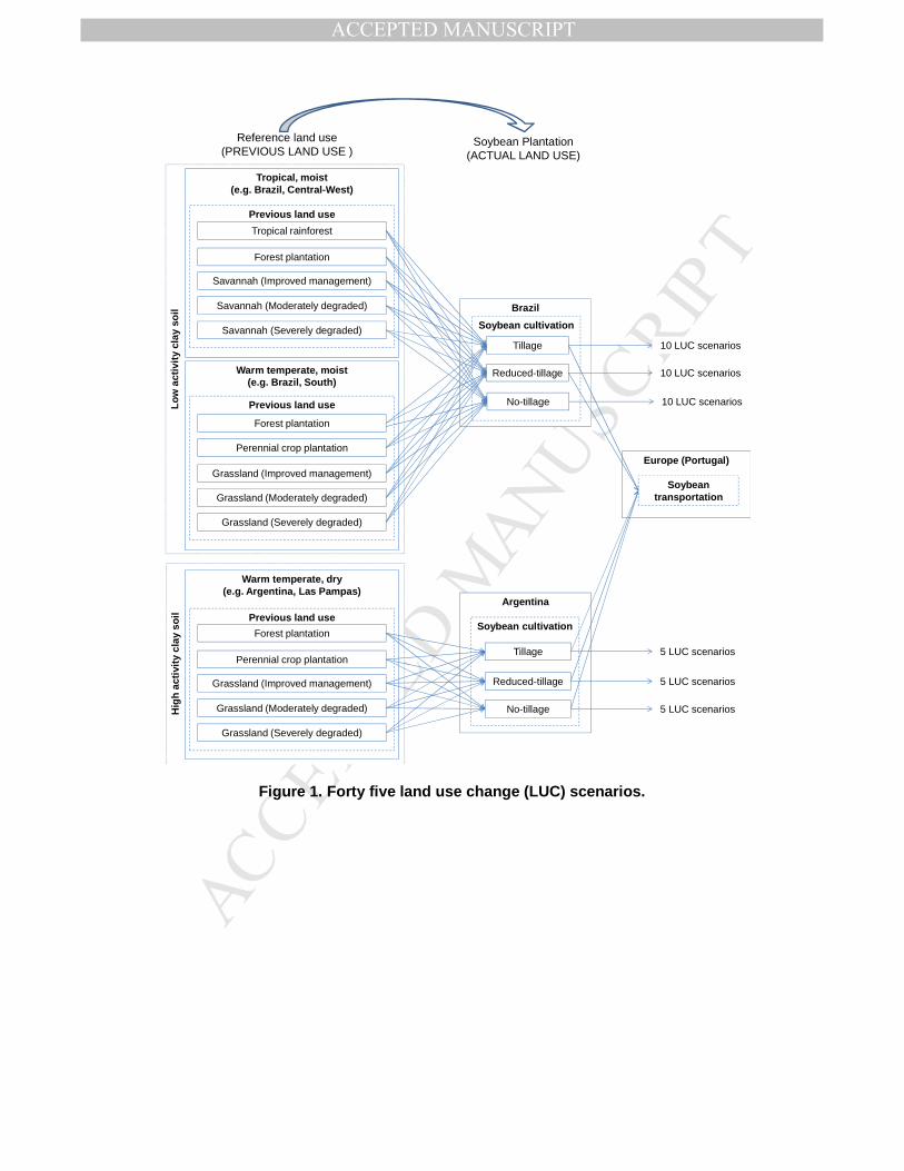
Fig. 1 shows the 45 LUC scenarios. These scenarios were established on the basis of
a combination of alternative previous land uses (conversion of tropical forest land,
forest plantations, perennial crop plantations, savannah and grasslands), different
cultivation systems (tillage, reduced tillage and no-tillage), climate (tropical moist, and
warm temperate, moist and dry) and soil characteristics (low and high activity clay
soils). Three climate regions and two soil types were selected because they represent
the most important area in LA (Brazil and Argentina) where soybean is produced. In
Brazil (2009/2010) about 83% of soybean was produced in the Central-West (tropical
moist climate) and South (warm temperate moist climate) regions, which are
characterized by low activity clay soils (IBGE, 2012; European Commission, 2010b). In
Argentina, about 76% of soybean (2009/2010) was produced in the provinces of
Buenos Aires, Córdoba and Santa Fé in the Las Pampas region, characterized by a
warm temperate dry climate and high activity clay soils (Product Board MVO, 2011;
European Commission, 2010b). Concerning savannahs and grasslands conversion,
different management options were also included, namely improved management (IM),
moderately degraded (MD) and severely degraded (SD).

MANUSCRIP
T
ACCEPTED
ACCEPTED MANUSCRIPT
Forty-five scenarios were considered, since the soybean area increased significantly
during the period 1991-2011 in Brazil (9.6 to 23.9 Mha) and Argentina (4.8 to 18.8
Mha) (FAO, 2012). Panichelli et al. (2009) showed that in Argentina the expansion of
the soybean area from 2000 to 2005 occurred in former cropland (32%), pasture land
(27%), savannas (19%) and forests (22%). Regarding soybean expansion in Brazil,
Macedo et al. (2012) showed that from 2001 to 2005 this took place in rainforest land
(26%) and scrubland (74%) and from 2005 to 2009 mainly in scrubland (91%).
Moreover, Dros (2004) forecasted the expansion of the soybean area in Brazil and
Argentina up to 2020 as 13.2 Mha in Brazil and 5.4 Mha in Argentina.
Figure 1 about here
GHG emissions from carbon stock changes caused by LUC were calculated using Eq.
(1), following the IPCC Tier 1 and Renewable Energy Directive (IPCC, 2006; European
Commission, 2009, 2010b). Annualized GHG emissions from carbon stock change due
to LUC were found by dividing by the time period in which C pools are expected to
reach equilibrium after land-use conversion (IPCC default: 20 years).
PCSCSe ARl /120/112/44)( ×××−= (1)
in which el (t CO2eqt-1 soybean) are the annualized GHG emissions from carbon stock
change due to LUC; CSR (t C ha-1) is the carbon stock associated with the reference
(previous) land use; CSA (t C ha-1) is the carbon stock associated with the actual land
use (soybean cultivation) and P (t soybean ha-1 year-1) is the productivity. In order to
calculate CSR and CSA, Eq. (2) was applied
ii vegIiMGLUiSTvegiii CFFFSOCCSOCCS +×××=+= )( (2)
in which SOCi (t Cha-1) is the soil organic carbon in the reference (SOCR) and actual
land use (SOCA), Cvegi (t C ha-1) is the above and below ground vegetation carbon stock
in living biomass and in dead organic matter in the reference (CvegR) and actual land
use (CvegA), SOCST (t Cha-1) is the standard soil organic carbon and FLU, FMG and FI are
MANUSCRIP
T
ACCEPTED
ACCEPTED MANUSCRIPT
factors that reflect the difference in SOCST associated with the type of land use (FLU),
principle management practice (FMG) and different levels of carbon input to soil (FI).
Table 1 presents the SOCR, calculated, as well as the CvegR and FLU, FMG, FI factors
adopted from the European Commission (2010b). Regarding actual land use, CvegA is
equal to zero (since soybean is harvested annually). Table 2 presents the SOCA
calculated and the FLU, FMG, FI factors adopted (European Commission, 2010b). SOCST
values were selected for the 3 aforementioned climate regions and 2 types of soils.
Table 1 about here
Table 2 about here
2.2 Soybean cultivation systems
Alternative life-cycle inventories (LCI) for different soybean cultivation systems in Brazil
and Argentina were implemented, based on transparent studies providing important
quantitative information (FNP, 2012; Cavalett and Ortega, 2009, 2010; Ortega et al.
2005; Dalgaard et al., 2008; Panichelli et al., 2009). Table 3 shows the annual
production and main inputs of 3 types of cultivation in Brazil and Argentina: no-tillage
(NT), reduced tillage (RT) and tillage (T). It should be noted that NT is now widespread
in Brazil and Argentina (more than 70%).
Table 3 about here
The LCI for NT soybean cultivation in Brazil was based on official data for agricultural
operations and inputs for transgenic Roundup Ready (RR) soybean production in
Paraná state (FNP, 2012). In Paraná, more than 90% of soybean is RR produced
under NT. An RT LCI was adopted from Cavalett and Ortega (2009, 2010). For
soybean cultivation under tillage in Brazil, an LCI was produced based on the intensive
system described by Ortega et al. (2005), characterized by the intensive use of
pesticides and agricultural machinery. Pesticide use was calculated based on the input
data and information on individual trade products, doses and main active ingredients.
The type of fertilizers used in soybean plantations was adopted from Brazilian statistics

MANUSCRIP
T
ACCEPTED
ACCEPTED MANUSCRIPT
for the fertilizers sector. The diesel consumption considered for the NT soybean system
was calculated based on the specific consumption for agricultural operations provided
by Romanelli et al. (2012). In all cultivation systems, a residual effect of lime application
for 5 years was considered; the values shown in Table 3 are the corresponding annual
values.
The main inputs of NT soybean production in Argentina were based on the LCI
presented by Dalgaard et al. (2008). Concerning RT and T soybean production in
Argentina, the LCI data was adopted from Panichelli et al. (2009), but adjustments
were made for soybean yields and pesticides. The yields were calculated for RT (2677
kgha-1) and T (2248 kgha-1) based on the average yield of 2591 kgha-1 and the
respective RT and T shares in national production (79.9% and 20.1%) (Panichelli et al.,
2009). It was also considered that the soybean yield is about 17%-20% higher under
RT than T systems, based on information for cultivation in other countries (Opara-Nadi,
1993). Regarding pesticides, it was considered that pesticide use is higher in RT
systems (Deike et al., 2008; Friedrich, 2005), in particular the use of herbicides (2,4D is
typically consumed in RT) (Tosi et al., 2005). The use of glyphosate was calculated as
the weighted quantity of glyphosate for both systems, considering the national shares
of RT and T production systems (79.9% and 20.1%).
2.2.1 GHG emissions: agricultural operations and field emissions
Regarding GHG emissions from soybean cultivation, diesel combustion from
agricultural operations (mainly CO2, calculated based on Nemecek et al. (2007))
together with field CO2 emissions from liming (IPCC, 2006) and N2O emissions (from N
additions to soils and mineralization of N in soil organic matter following land-use
change in mineral soils) were considered. GHG emissions associated with the
production of agricultural inputs were also accounted for using emission factors for
pesticides (Nemecek et al., 2007), limestone (Kellenberger et al., 2007), fertilizers
(Patyk and Reinhardt, 1997; Nemecek et al., 2007) and diesel (Jungbluth, 2007).

MANUSCRIP
T
ACCEPTED
ACCEPTED MANUSCRIPT
The IPCC Tier 1 methodology (IPCC, 2006) was used to calculate direct and indirect
N2O emissions. Direct N2O emissions occur directly from the soils to which the N is
added/released (from anthropogenic N inputs or N mineralization). Indirect N2O
emissions occur through two pathways (IPCC, 2006): i) following volatilization of NH3
and NOx from the soil and the subsequent deposition of these gases and their products
(NH4+ and NO3
-) to soils and waters and ii) after leaching and runoff of N, mainly as
NO3-. Direct and indirect N2O emissions were calculated using Eq. (3) and (4) (IPCC,
2006) for each alternative cultivation system,
28/44)( 12 ××++= EFFFFON SOMCRSNDirect (3)
[ ] 28/44))(( 542 ×××+++××= EFFracFFFEFFracFON LEACHSOMCRSNGASFSNIndirect (4)
in which FSN is the annual amount of synthetic fertilizer N applied to soils (kg N ha-1),
FCR is the annual amount of N in crop residues (above-ground and below-ground)
returned to soils (kg N ha-1), FSOM is the annual amount of N in mineral soils that is
mineralized (the process by which organic N in soil organic matter is converted to
inorganic forms: NH4+ and NO3
-), in association with loss of soil C from soil organic
matter as a result of changes to land use or management (kg N ha-1). Organic C and N
are closely linked in soil organic matter and when soil C is lost through oxidation as a
result of LUC, this loss will be accompanied by a simultaneous mineralization of N
(IPCC, 2006). EF1, EF4 and EF5 are the emission factors adopted for N2O emissions
from N additions (kg N2O-N kg-1 N input), from atmospheric deposition of N on soils
and water surfaces (kg N2O-N (kg NH3–N+NOx-N volatilized)-1) and from N leaching
and runoff (kg N2O–N (kg N leached and runoff)-1), respectively. FracGASF is the fraction
of FSN that volatilizes as NH3 and NOx, kg N volatilized kg-1 N applied and FracLEACH is
the fraction of all N added to/mineralized in managed soils in regions where
leaching/runoff occurs that is lost through leaching and runoff (kg N kg-1 N additions).
The amounts of N added/released (FSN, FCR and FSOM), default emission factors (EF1,
EF4 and EF5), fractions that volatilize (FracGASF) and are lost through leaching and
MANUSCRIP
T
ACCEPTED
ACCEPTED MANUSCRIPT
runoff (FracLEACH) are presented in Table 4 (uncertainty ranges presented inside
brackets). FSN is equal to zero in all systems except RT and T in Argentina, where
synthetic N is applied as monoammonium phosphate. The amount of N in crop
residues (FCR) was estimated on the basis of the soybean yield and default factors for
above-/below-ground residue given by the IPCC (2006). The N2O emissions from N
mineralization as a result of loss of soil carbon through changes in land use and
management (FSOM) were estimated on the basis of the average annual loss of soil
carbon for each LUC scenario and a default C:N ratio of 15. It should be noted that the
2006 IPCC guidelines included significant adjustments to the methodology previously
described in the 1996 IPCC guidelines: i) biological nitrogen fixation was removed as a
direct source of N2O (after Rochette and Janzen (2005) concluded that N2O emissions
induced by the growth of legume crops may be estimated solely as a function of the
above-ground and below-ground nitrogen inputs from crop residue) and ii) the release
of N by mineralization of soil organic matter as a result of change of land use or
management was included as an additional source.
Table 4 about here
2.3 Soybean transportation
The transportation of soybean from the plantations in Brazil and Argentina to Europe
encompasses transport by lorry (“16-32t”) to the ports and by transoceanic freighter to
the port of Lisbon (Portugal). It was assumed that the type of lorry complies with EURO
3 (European Union emission standards for vehicles, Directive 98/69/EC). The GHG
emissions from transoceanic and road transportation were calculated based on
emissions factors (Spielmann et al., 2007) and distances between the different places
of origin of the soybean and the port of Lisbon. The distances from Brazil and
Argentina to the port in Portugal were 8371 km and 10244 km, respectively. The
distances were estimated on the basis of the distances presented in Table 5 and the
quantity exported from each port (the weighted average distance). In Brazil (in 2010),

MANUSCRIP
T
ACCEPTED
ACCEPTED MANUSCRIPT
about 85% of soybean was exported from the ports of Santos (25%), Paranaguá
(36%), Rio Grande (16%) and Vitória (8%) (Silva, 2010). In Argentina, 75% of the
soybean was exported (the average for 2009-2010) from Bahia Blanca (30%), Rosario
(24%) and San Lorenzo/San Martin (21%)(MAGyP, 2012).
Table 5 about here
Regarding the transport of soybean from the plantations to the ports, the distances of
1456 km and 403 km were adopted for Brazil and Argentina, respectively. These
weighted average distances were calculated based on the distances between the main
ports and the main soybean producing locations (IBGE, 2012; SIIA, 2012) presented in
Tables 6 (Brazil) and 7 (Argentina), as well as the percentage of soybean production
and exportation (shown in brackets in Tables 6 and 7) in relation to national production.
The influence of locations on soybean GHG emissions was assessed based on the use
of maximum and minimum distances between plantations and ports. The effect of the
type of lorry was analyzed based on the GHG emission factors for eleven types of lorry,
using a combination of different capacities (in tonnes) and standards for vehicles
(EURO 3, 4, 5 and fleet average): >16t (fleet average), >32t (EURO3, 4, 5), 16-32t
(EURO3, 4, 5), 3,5-16t (fleet average), 7,5-16t (EURO3, 4, 5).
Table 6 about here
Table 7 about here
3 Results and discussion
The main results are presented and discussed in this section, which provides a GHG
assessment of soybean for the 45 different LUC scenarios and cultivation systems,
including an analysis of the contribution of each LC stage and GHG type. It also
provides a sensitivity analysis of field N2O emissions and transportation routes.
MANUSCRIP
T
ACCEPTED
ACCEPTED MANUSCRIPT
3.1 The LC GHG balance for soybean
Fig. 2 presents the GHG balance (LUC, cultivation and transportation), calculated on
the basis of average soybean transportation distances, as well as default parameters
and emission factors for field N2O emissions. A huge variation can be observed,
ranging from 0.06 to 17.8 kg CO2eq kg-1 of soybean. The highest GHG emissions were
calculated for the tropical (moist) region when tropical rainforest is converted into
soybean plantations (tillage system). On the other hand, the lowest GHG emissions
were calculated for severely degraded grasslands in the warm temperate (dry) region.
LUC dominates the results, contributing significantly to the GHG balance in almost all
scenarios. LUC represents more than 70% in 28 scenarios (all tropical region
scenarios, with 9 out of 15 in warm temperate moist regions and 9 out of 15 in warm
temperate dry regions). LUC amounts to less than 45% in the scenarios in which
severely degraded grassland has been converted in warm temperate regions. In warm
temperate dry regions, negative CO2 emissions due to LUC were obtained (-0.06 to -
0.26 kg CO2eq kg-1), due to the fact that the SOCA in the soybean plantations is higher
than the SOCR in the severely degraded grassland in this region.
According to Dros (2004), 75% of land conversion in Brazil will take place in
savannah/shrubland (Cerrado in Central-West of Brazil) and 90% of the conversion in
Argentina in dry and moist savannah/grassland (Chaco). The LUC carbon stock
changes obtained for all grassland conversion scenarios in the warm temperate dry
region (Argentina) are lower than 1.5 kg CO2eq kg-1. In the tropical region (Brazil,
Central-West), the LUC carbon stock changes calculated for savanna/scrubland
(Cerrado) conversion vary between 3.5 and 7.0 kg CO2eq kg-1.
Some studies account for carbon emissions from direct LUC in the LC GHG
assessment of soybean and soybean-based products, although a wide range of results
has been reported. Table 8 compares the results from different articles. In order to
make the comparisons, the GHG intensity of soybean obtained in this article was
additionally calculated in terms of the GHG intensity of soybean-based biodiesel,

MANUSCRIP
T
ACCEPTED
ACCEPTED MANUSCRIPT
assuming the following: 5 kg soybean kg-1 biodiesel (Panichelli et al., 2009); emissions
from processing 18 g CO2eq MJ-1(European Commission, 2009); an energy allocation
factor of 34% (36% for oil extraction and 95% for transesterification) (Castanheira and
Freire, 2012). In general, the results from the various publications that addressed LUC
showed a huge variation in GHG intensity. The lowest results were obtained for
converted grassland and the highest for converted tropical forest and perennial
cropland.
Figure 2 about here
Table 8 about here
LUC emissions in Fig. 2 are disaggregated in ∆SOC and ∆Cveg, to allow for a better
understanding of the contribution of soil and vegetation carbon stock changes to the
overall GHG balance. More than 50% of the LUC CO2 emissions occur due to a high
carbon stock change in vegetation (∆Cveg) in the following 24 scenarios: i) all LUC
scenarios in the tropical region, ii) forest and perennial crop conversions in warm
temperate regions, iii) severely and moderately degraded grassland conversion in
warm temperate moist and dry regions. Changes in SOC (∆SOC) contribute more than
50% to LUC CO2 emissions in the 12 remaining scenarios.
Concerning cultivation, it can be observed that tillage systems have higher GHG
emissions than the corresponding reduced or no-tillage systems in each region. The
lowest GHG emissions occur when soybean is cultivated using reduced and no-tillage
in former grassland in the warm temperate dry region (less than 2.2 kg CO2eq kg-1).
Batlle-Bayer et al. (2010) also showed that no-till practices reduce soil organic carbon
losses (0-30 centimeter topsoil layer) after land use conversion from conventional
tillage (primary and secondary tillage). According to the Product Board MVO (2011),
the main reason is that no-till farming protects the soil from erosion and structural
breakdown. No-tillage offers the possibility not only of reducing carbon loss from the
soil as a result of cultivation, but also of increasing soil carbon in the form of organic

MANUSCRIP
T
ACCEPTED
ACCEPTED MANUSCRIPT
matter, with positive impacts on both soil productivity and GHG reductions (Cavalett
and Ortega, 2009, 2010).
GHG emissions from the cultivation and transport of soybean vary between 0.3 and 0.9
kg CO2eq kg-1 soybean. The contribution of cultivation ranges from 2% (rainforest
conversion in the tropical region, NT soybean) to 53% (no LUC in all regions, T
soybean). Transportation represents between 2% (rainforest conversion in the tropical
region in all soybean cultivation systems) and 60% (no LUC in tropical and warm
temperate moist regions, NT soybean) of the total GHG emissions. When LUC is not
considered, the contribution of cultivation varies between 40%-49% (no- and reduced
tillage) and 53% (tillage) for the alternative systems, whereas transportation contributes
47%-60% to the total soybean GHG emissions.
3.2 GHG emissions from soybean cultivation
GHG emissions for the alternative cultivation systems (including the contribution of
main inputs) are shown in Fig. 3. N2O emissions from N mineralization (as a result of
loss of soil carbon due to LUC) are not presented in Fig. 3. GHG emission ranges for
cultivation obtained from the sensitivity analysis performed for field N2O emissions
(maximum and minimum parameters and emission factors) are presented in the chart
as error (range) bars. GHG emissions for soybean cultivation, adopting default values
in the calculation of field N2O emissions, vary between 0.14 (reduced-tillage, Argentina)
and 0.32 kg CO2eq kg-1 (tillage, Brazil). These results can be justified by the higher
soybean yields and lower diesel requirements (for machinery) in no- and reduced
tillage, since direct seeding is performed without primary tillage.
Figure 3 about here
The great variation in GHG emissions presented in Fig. 3 for the soybean cultivation
systems can be explained by the variation in fertilizer, lime and diesel inputs. Soybean
cultivation in tropical and warm temperate moist regions has higher GHG emissions
(0.19-0.32 kg CO2eq kg-1) compared to the warm temperate dry regions (0.14-0.19 kg

MANUSCRIP
T
ACCEPTED
ACCEPTED MANUSCRIPT
CO2eq kg-1). This difference is due to the use of limestone and greater quantities of
fertilizer in Brazil. Field N2O emissions (default) are the most important contributions to
the GHG emissions from cultivation (between 32% and 58%) except under the tillage
system in Brazil, where the emissions from the use of machinery contribute 37%.
Diesel for agricultural machinery represents 25% to 45% of the total emissions, with a
higher contribution under tillage systems than the corresponding no- or reduced tillage
systems. The main reason for the variations in GHG emissions in the cultivation
systems is diesel consumption, although the reason for the different GHG results from
Brazil and Argentina is the amount of fertilizer and lime applied to the soil.
Regarding the sensitivity analysis of the field N2O emissions, it can be observed that
the uncertainty in N2O emission calculations is very high and dominates GHG
cultivation emissions. When minimum parameters and emission factors are adopted,
the emissions from cultivation are reduced by 19% to 44%. If the maximum parameters
and emission factors are adopted, cultivation emissions increase by 80% to 181% and
the field N2O emissions dominate (59% to 85%) the results for all cultivation systems.
These results show that GHG emissions from cultivation are very sensitive to the
parameters and emission factors adopted for field N2O emissions calculations. This
concurs with other studies, showing that field N2O emissions play a major role in the
GHG emissions from soybean cultivation.
An analysis of the contribution of each GHG (CO2, N2O and CH4) to the overall
soybean GHG emissions produced by the various cultivation systems (expressed in
CO2 equivalents) is presented in Fig. 4. When default N2O emissions are considered,
CO2 emissions from diesel combustion and the production of fertilizers are the main
factors contributing to the GHG intensity for soybean produced in tropical and warm
temperate moist regions. N2O contributes less than 41% in these regions, but more
than 47% in warm temperate dry regions (due to field N2O emissions). However, when
minimum values are adopted for the field N2O emissions, the results are significantly
different and CO2 represents a higher contribution to cultivation emissions in all regions

MANUSCRIP
T
ACCEPTED
ACCEPTED MANUSCRIPT
(72-89%). It can also be observed that if maximum values are adopted 59% to 85% of
GHG emissions are due to N2O. Methane emissions represent less than 3% in all the
scenarios considered.
Figure 4 about here
3.3 Soybean transportation
Fig. 5 shows the GHG transportation emissions, calculated on the basis of the
weighted average distances for the transoceanic and road transportation of soybean.
The error range bars represent the variation associated with eleven types of lorry and
the maximum and minimum distances for each route. The highest emissions were
calculated for the “3.5-16 t” lorry (fleet average) and the lowest for the “>32t” lorry
(EURO4). Transportation of soybean from Brazil involves higher emissions (0.29 kg
CO2eq kg-1 soybean) than Argentina (0.16 kg CO2eq kg-1 soybean) due to the greater
road transport distances in Brazil. About 69% of the emissions in Brazil are from road
transportation, whereas in Argentina this only represents 34% of the total transportation
emissions. In Brazil, soybean exported from Mato Grosso has higher GHG emissions
than other states. Regarding ports, it can be observed that the emissions are in general
lower for soybean exported from Santos and Paranaguá. In Argentina, no significant
differences in the results were observed.
Figure 5 about here
4 Conclusions
This article presents an assessment of the LC GHG emissions from soybean produced
in Latin America, focusing on the implications of different cultivation systems and direct
LUC. An LC model and inventories for soybean produced in Brazil and Argentina was
developed, addressing LUC, cultivation and transport to Europe. A comprehensive
evaluation of 45 scenarios, resulting from a combination of LUC and cultivation
systems for Brazil and Argentina, was undertaken. The results demonstrate the

MANUSCRIP
T
ACCEPTED
ACCEPTED MANUSCRIPT
importance of LUC in the soybean GHG balance, although significant GHG variation
was observed for the alternative LUC and cultivation systems assessed. The highest
GHG emissions (17.8 kg CO2eqkg-1) were calculated for the tropical region when
tropical rainforest is converted into soybean cultivation (the tillage system). On the
other hand, the lowest GHG emissions were calculated for severely degraded
grassland in Argentina (0.1 to 0.3 kg CO2eqkg-1), due to an increase in the SOC of
soybean cultivation in relation to the SOC of severely degraded grassland (the
reference land use). Concerning soil management practices, it was observed that all
the tillage systems have higher GHG emissions than the corresponding reduced tillage
and no-tillage systems. A sensitivity analysis for N2O emission calculations was also
presented, showing a high level of uncertainty in the calculation of N2O emissions.
Acknowledgments
The research presented in this article was supported by the Portuguese Foundation for
Science and Technology (FCT) projects MIT/SET/0014/2009 (Capturing Uncertainty in
Biofuels for Transportation. Resolving Environmental Performance and Enabling
Improved Use) and PTDC/SEN-TRA/117251/2010 (Extended “well-to-wheels”
assessment of biodiesel for heavy transport vehicles). The study also forms part of the
Energy for Sustainability Initiative at the University of Coimbra (www.uc.pt/efs) and the
MIT-Portugal program. Érica Castanheira gratefully acknowledges financial support
from the FCT, through grant SFRH/BD/60328/2009.
References
Alvarenga, R. A. F., Júnior, V. S., Soares, S. R., 2012. Comparison of the ecological
footprint and a life cycle impact assessment method for a case study on Brazilian
broiler feed production. Journal of Cleaner Production 28, 25-32.

MANUSCRIP
T
ACCEPTED
ACCEPTED MANUSCRIPT
Basset-Mens, C., van der Werf, H.M.G., Robin, P., Morvan, Th., Hassouna, M., Paillat,
J.-M., Verte`s, F., 2007. Methods and data for the environmental inventory of
contrasting pig production systems. Journal of Cleaner Production 15, 1395-1405.
Batlle-Bayer, L., Batjes, N. H., Bindraban, P. S., 2010. Changes in organic carbon
stocks upon land use conversion in the Brazilian Cerrado: A review. Agriculture,
Ecosystems and Environment 137, 47–58.
Börjesson, P., Tufvesson, L. M., 2011. Agricultural crop-based biofuels – resource
efficiency and environmental performance including direct land use changes. Journal of
Cleaner Production 19, 108–120.
Brandão, M., Clift, R., Milà i Canals, L., Basson, L., 2010. A Life-Cycle Approach to
Characterising Environmental and Economic Impacts of Multifunctional Land-Use
Systems: An Integrated Assessment in the UK. Sustainability 2, 3747-3776.
Castanheira, E. G., Freire F., 2012. Life-cycle GHG assessment of soybean biodiesel.
Proceedings of the 2012 IEEE International Symposium on Sustainable Systems and
Technology (ISSST), Boston, 16-18 May 2012, 1-5.
Cavalett, O., Ortega, E., 2010. Integrated environmental assessment of biodiesel
production from soybean in Brazil. Journal of Cleaner Production 18, 55-70.
Cavalett, O., Ortega, E., 2009. Emergy, nutrients balance and economic assessment of
soybean production and industrialization in Brazil. Journal of Cleaner Production 17,
762-771.
Chamberlain, J.F., Miller, S.A., Frederick, J.R., 2011. Using DAYCENT to quantify on-
farm GHG emissions and N dynamics of land use conversion to N-managed
switchgrass in the Southern U. S. Agriculture, Ecosystems and Environment 141, 332-
341.
Cherubini, F., 2010. GHG balances of bioenergy systems – Overview of key steps in
the production chain and methodological concerns. Renewable Energy 35, 1565–1573.
Dalgaard, R., Schmidt, J., Halberg, N., Christensen, P., Thrane, M., Pengue, W. A.,
2008. LCA of Soybean Meal. Int. J. Life Cycle Assess. 3, 240-254.

MANUSCRIP
T
ACCEPTED
ACCEPTED MANUSCRIPT
Deike, S., Pallutt, B., Melander, B., Strassemeyer, J., Christen, O., 2008. Long-term
productivity and environmental effects of arable farming as affected by crop rotation,
soil tillage intensity and strategy of pesticide use: A case-article of two long-term field
experiments in Germany and Denmark. Europ. J. Agronomy 29, 191–199.
Del Grosso, S.J., Ojima, D.S., Parton, W.J., Stehfest, E., Heistemann, M., DeAngelo,
B., Rose, S., 2009. Global scale DAYCENT model analysis of greenhouse gas
emissions and mitigation strategies for cropped soils. Global Planetary Change 67, 44-
50.
Dros J.M., 2004. Managing the soy boom: Two scenarios of soy production expansion
in South America. Report commissioned by the World Wild Life Fund, Available at:
http://assets.panda.org/downloads/managingthesoyboomenglish_nbvt.pdf (accessed 5
March 2012).
European Commission, 2009. Directive 2009/28/EC of the European Parliament and of
the council of 23 April 2009 on the promotion of the use of energy from renewable
sources and amending and subsequently repealing Directives 2001/77/EC and
2003/30/EC, Official Journal of the European Union, L140/16 of 5.6.2009.
European Commission, 2010a. Report from the Commission on indirect land-use
change related to biofuels and bioliquids, COM (2010) 811 final, Brussels, 22.12.2010.
European Commission, 2010b. Commission Decision of 10 June 2010 on guidelines
for the calculation of land carbon stocks for the purpose of Annex V to Directive
2009/28/EC, Official Journal of the European Union, L151/19 of 17.6.2010.
FAO, 2012. FAO STAT. FAOSTAT agriculture data, food and agriculture organisation
of the United Nations, 2012. Available at: http://faostat.fao.org/
Flysjö, A., Cederberg, C., Henriksson, M., Ledgard, S., 2012. The interaction between
milk and beef production and emissions from land use change e critical considerations
in life cycle assessment and carbon footprint studies of milk. Journal of Cleaner
Production 28, 134-142.

MANUSCRIP
T
ACCEPTED
ACCEPTED MANUSCRIPT
FNP, 2012. Agrianual 2011: Anuário da Agricultura Brasileira. FNP Consultoria e
Comércio - São Paulo.
Friedrich, T., 2005. Does No-till Farming require more herbicides? Outlooks on Pest
Management, 188-191.
Hokazono, S., Hayashi, K., 2012. Variability in environmental impacts during
conversion from conventional to organic farming: a comparison among three rice
production systems in Japan. Journal of Cleaner Production 28, 101-112.
Huo, H., Wang, M., Bloyd, C., Putsche, V., 2009. Life-cycle assessment of energy use
and greenhouse gas emissions of soybean-derived biodiesel and renewable fuels.
Environ. Sci. Technol. 43, 750-756.
Huo, H., Wang, M., Bloyd, C., Putshe, V., 2008. Life-Cycle Assessment of Energy and
Greenhouse Gas Effects of Soybean-Derived Biodiesel and Renewable Fuels. Work
sponsored by the U.S. Department of Energy, Office of Energy Efficiency and
Renewable Energy, March 12, 2008.
IBGE, 2012. Produção Agrícola Municipal. Área plantada, área colhida, quantidade
produzida e valor da produção da lavoura temporária. Instituto Brasileiro de Geografia
e Estatística - IBGE. Available at: http://www.sidra.ibge.gov.br (accessed August 10,
2012).
IPCC, 2007. IPCC Fourth Assessment Report: Climate Change 2007, Contribution of
Working Group I to the 4th Assessment Report of the IPCC, Cambridge University
Press, USA.
IPCC, 2006. IPCC guidelines for national greenhouse gas inventories. Prepared by the
National Greenhouse Gas Inventories Programme, Eggleston, H.S., Buendia, L., Miwa,
K., Ngara, T., Tanabe, K. (Eds.). Hayama, Japan: Institute for Global Environmental
Strategies.
ISO, 2006. Environmental management - Life cycle assessment - Principles and
framework, ISO 14040. International Organization for Standardization, Geneva,
Switzerland.

MANUSCRIP
T
ACCEPTED
ACCEPTED MANUSCRIPT
Jungbluth, N., 2007. Erdöl. Sachbilanzen von Energiesystemen. Final report No. 6
ecoinvent data v2.0, Editors: Dones R., Vol. 6, Swiss Centre for LCI, PSI, Dübendorf
and Villigen.
Kellenberger, D., Althaus, H.-J., Jungbluth, N., Künniger, T., 2007. Life Cycle
Inventories of Building Products. Final report ecoinvent data v2.0, Vol. 7, Swiss Centre
for LCI, Empa – TSL, Dübendorf.
Kendall, A., Chang, B., 2009. Estimating life cycle greenhouse gas emissions from
corn-ethanol: a critical review of current U.S. practices. Journal of Cleaner Production
17, 1175-1182.
Kim, S., Dale, B. E., 2009. Regional variations in greenhouse gas emissions of
biobased products in the United States—corn-based ethanol and soybean oil. Int. J. of
Life Cycle Assess. 14, 540–546.
Knudsen, M. T., Yu-Hui, Q., Yan, L., Halberg, N., 2010. Environmental assessment of
organic soybean (Glycine max.) imported from China to Denmark: a case study.
Journal of Cleaner Production 18, 1431-1439.
Krautgartner, R., Henard, M.C., Rehder, L. E., Boshnakova, M., Dobrescu, M., Flach,
B., Wilson, J., Wideback, A., Bettini, O., Guerrero, M., Bendz, K., 2012. EU-27
Oilseeds and Products Annual. USDA Foreign Agricultural Service: GAIN-Global
Agricultural Information Network. GAIN Report Number: E70016.
Landis, A.E., Miller, S. A., Theis, T. L., 2007. Life Cycle of the Corn-Soybean
Agroecosystem for Biobased Production. Environ. Sci. Technol. 41, 1457-1464.
Lehuger, S., Gabrielle, B., Gagnaire, N., 2009. Environmental impact of the substitution
of imported soybean meal with locally-produced rapeseed meal in dairy cow feed.
Journal of Cleaner Production 17, 616–624.
Macedo, M. N., DeFries, R. S., Morton, D. C., Stickler, C. M., Galford, G. L.,
Shimabukuro, Y. E., 2012. Decoupling of deforestation and soy production in the
southern Amazon during the late 2000s. Proceedings of the National Academy of
Sciences 109(4), 1341-1346.

MANUSCRIP
T
ACCEPTED
ACCEPTED MANUSCRIPT
MAGyP, 2012. Exportaciones de Granos, Aceites y Subproductos - Volúmenes
exportados de granos. Ministerio de Agricultura, Ganadería y Pesca-MAGyP. Available
at: http://www.minagri.gob.ar (accessed August 10, 2012).
Miller, S.A., 2010. Minimizing Land Use and Nitrogen Intensity of Bioenergy. Environ.
Sci. Technol. 44, 3932–3939.
Miller, S., Landis, A., Theis, T., Reich, R., 2007. A Comparative Life Cycle Assessment
of Petroleum and Soybean-Based Lubricants. Environ. Sci. Technol. 41, 4143-4149.
Miller, S., Landis, A., Theis, T., 2006. Use of Monte Carlo Analysis to Characterize
Nitrogen Fluxes in Agroecosystems. Environ. Sci. Technol. 40, 2324-2332.
Mourad, A. L., Walter, A., 2011. The energy balance of soybean biodiesel in Brazil: a
case article. Biofuels, Bioproducts and Biorefinery 5, 185–197.
Nemecek, T., Kägi, T., Blaser, S., 2007. Life Cycle Inventories of Agricultural
Production Systems. Ecoinvent report version 2.0, Vol. 15, Swiss Centre for LCI, ART,
Duebendorf and Zurich.
Omni Tech International, 2010. Life Cycle Impact of Soybean Production and Soy
Industrial Products. Prepared for The United Soybean Board (USB) by Omni Tech
International. Released February 2010.
Opara-Nadi, O.A., 1993. Chapter 8 - Conservation tillage for increased crop production,
in: FAO (Ed), Soil tillage in Africa: needs and challenges. FAO Soils Bulletin 69.
Ortega, E., Cavalett, O., Bonifácio, R., Watanabe, M., 2005. Brazilian soybean
production: emergy analysis with an expanded scope. Bulletin of Science, Technology
& Society 25, 323-334.
Panichelli, L., Dauriat, A., Gnansounou, E., 2009. Life cycle assessment of soybean-
based biodiesel in Argentina for export. Int. J. of Life Cycle Assess. 14, 144-159.
Patyk, A., Reinhardt, G., 1997. Düngemittel - Energie- und Stoffstromsbilanzen.
Vieweg. Umweltvissenschaften. Friedr. Vieweg & Sohn Verlagsgesellschaft mbH,
Braunschweig/Wiesbaden, Germany.

MANUSCRIP
T
ACCEPTED
ACCEPTED MANUSCRIPT
Ponsioen, T.C., Blonk, T.J., 2012. Calculating land use change in carbon footprints of
agricultural products as an impact of current land use. Journal of Cleaner Production
28, 120-126.
Product Board MVO, 2011. Fact sheet Soy. Rijswijk, The Netherlands: Product Board
Margarine, Fats and Oils.
Prudêncio da Silva, V., van der Werf, H. M. G., Spies, A., Soares, S. R., 2010.
Variability in environmental impacts of Brazilian soybean according to crop production
and transport scenarios. Journal of Environmental Management 91, 1831-1839.
Reijnders, L., Huijbregts, M.A.J., 2011. Nitrous oxide emissions from liquid biofuel
production in life cycle assessment. Current Opinion in Environmental Sustainability 3,
432–437.
Reijnders, L., Huijbregts, M.A.J., 2008. Biogenic greenhouse gas emissions linked to
the life cycles of biodiesel derived from European rapeseed and Brazilian soybeans.
Journal of Cleaner Production 16, 1943-1948.
Reinhard, J., Zah, R., 2009. Global environmental consequences of increased
biodiesel consumption in Switzerland: consequential life cycle assessment. Journal of
Cleaner Production 17, S46-S56.
Rochette, P., Janzen, H.H., 2005. Towards a revised coefficient for estimating N2O
emissions from legumes. Nutr. Cycl. Agroecosyst. 73, 171-179.
Romanelli, T. L., Nardi, H. S., Saad, F. A., 2012. Material embodiment and energy
flows as efficiency indicators of soybean (Glycine max) production in Brazil.
Engenharia Agrícola 32, 261-270.
Searchinger, T., Heimlich, R., 2009. Estimating greenhouse gas emissions from Soy-
Based US biodiesel when factoring in emissions from land use change. Biofuels, Food
and Feed Tradeoffs, 45-55.
SIIA, 2012. Producción Agrícola Por Provincias. Sistema Integrado de Información
Agropecuaria - SIIA, Ministerio de Agricultura, Ganadería y Pesca. Available at:
http://www.siia.gov.ar (accessed August 10, 2012).

MANUSCRIP
T
ACCEPTED
ACCEPTED MANUSCRIPT
Silva, G. S., 2010. Os Desafios da Soja no Brasil. Aprosoja- Associação dos
Produtores de Soja e Milho do Estado de Mato Grosso. FASUL – Faculdade Sul Brasil,
Maio 2010.
Smaling, E.M.A., Roscoe, R., Lesschen, J.P., Bouwman, A.F., Comunello E., 2008.
From forest to waste: Assessment of the Brazilian soybean chain, using nitrogen as a
marker. Agriculture, Ecosystems and Environment 128, 185–197.
Smeets, E.M.W., Bouwmanw, L.F., Stehfest, E., van Vuuren, D.P., Posthuma, A.,
2009. Contribution of N2O to the greenhouse gas balance of first-generation biofuels.
Global Change Biology 15, 1-23.
Snyder, C.S., Bruulsema, T.W., Jensen, T.L., Fixen, P.E., 2009. Review of greenhouse
gas emissions from crop production systems and fertilizer management effects.
Agriculture, Ecosystems and Environment 133, 247–266.
Spielmann, M., Dones, R., Bauer, C., 2007. Life Cycle Inventories of Transport
Services. Final report ecoinvent Data v2.0, Vol. 14, Dübendorf and Villigen,
Switzerland, Swiss Centre for LCI, PSI.
USDA, 2012. Soybean Oilseed Production, Exports and Imports by Country. USDA -
United States Department of Agriculture. Available at: http://www.indexmundi.com
(accessed August 14, 2012).
van Dam, J., Faaij, A.P.C., Hilbert, J., Petruzzi, H., Turkenburg, W.C., 2009. Large-
scale bioenergy production from soybeans and switchgrass in Argentina Part B.
Environmental and socio-economic impacts on a regional level. Renewable and
Sustainable Energy Reviews 13, 1679–1709.
Tosi, J., Mosciaro, M., Borda, M., Forján, H., Marinissen, A., Pereyra, E. S., 2005.
Haciendo numeros para la campaña 05/06 de soja. Instituto Nacional de Tecnología
Agropecuaria - INTA. Available at: http://riap.inta.gov.ar/ (accessed August 14, 2012).
Tsoutsos, T., Kouloumpis, V., Zafiris, T., Foteinis S., 2010. Life Cycle Assessment for
biodiesel production under Greek climate conditions. Journal of Cleaner Production 18,
328–335.

MANUSCRIP
T
ACCEPTED
ACCEPTED MANUSCRIPT
Figure captions:
Figure 1. The forty-five land use change (LUC) scenarios.
Figure 2. The soybean LC GHG balance: alternative LUC scenarios and cultivation
systems in 3 LA regions.
Figure 3.GHG emissions from alternative soybean cultivation systems.
Figure 4. Contribution of each GHG to total emissions from alternative cultivation
systems.
Figure 5.GHG emissions from soybean transportation.
MANUSCRIP
T
ACCEPTED
ACCEPTED MANUSCRIPT
Europe (Portugal)
Argentina
Brazil
Low
act
ivit
y cl
ay s
oil
Tropical, moist (e.g. Brazil, Central-West)
Previous land use
Hig
h ac
tivi
ty c
lay
soil
Tropical rainforest
Forest plantation
Savannah (Improved management)
Savannah (Moderately degraded)
Savannah (Severely degraded) Soybean cultivation
Tillage
Reduced-tillage
10 LUC scenarios
Warm temperate, moist(e.g. Brazil, South)
Previous land use
Forest plantation
Perennial crop plantation
Grassland (Improved management)
Grassland (Moderately degraded)
Grassland (Severely degraded)
Warm temperate, dry (e.g. Argentina, Las Pampas)
Previous land use
Forest plantation
Perennial crop plantation
Grassland (Improved management)
Grassland (Moderately degraded)
Grassland (Severely degraded)
Soybean cultivation
Tillage
Reduced-tillage
No-tillage
10 LUC scenarios
5 LUC scenarios
5 LUC scenarios
5 LUC scenarios
Reference land use(PREVIOUS LAND USE )
Soybean Plantation(ACTUAL LAND USE)
Soybean transportation
No-tillage 10 LUC scenarios
Figure 1. Forty five land use change (LUC) scenarios.

MANUSCRIP
T
ACCEPTED
ACCEPTED MANUSCRIPT
-1 1 3 5 7 9 11 13 15 17 19
NT
RT
T
NT
RT
T
NT
RT
T
NT
RT
T
NT
RT
T
NT
RT
T
NT
RT
T
NT
RT
T
NT
RT
T
NT
RT
T
NT
RT
T
NT
RT
T
NT
RT
T
NT
RT
T
NT
RT
T
NT
RT
T
NT
RT
T
NT
RT
T
Impr
oved
man
agem
ent
Mod
erat
ely
degr
aded
Sev
erel
yde
grad
edIm
prov
edm
anag
emen
tM
oder
atel
yde
grad
edS
ever
ely
degr
aded
Impr
oved
man
agem
ent
Mod
erat
ely
degr
aded
Sev
erel
yde
grad
ed
Tro
pica
lra
info
rest
For
est
plan
tatio
nS
avan
nah
(scr
ubla
nd)
No
LUC
For
est
plan
tatio
nP
eren
nial
crop
Gra
ssla
ndN
o LU
CF
ores
tpl
anta
tion
Per
enni
alcr
opG
rass
land
No
LUC
Life cycle GHG balance(kg CO2eq kg-1 soybean)
Transportation
Plantation
LUC (∆SOC)
LUC (∆Cveg)
Tropical (moist)
Warm temperate (moist)
Warm temperate (dry)
NT-No-tillage; RT-Reduced-tillage; T-Tillage
Figure 2. LC GHG balance of soybean: alternative LUC scenarios and cultivation systems
in 3 LA regions.

MANUSCRIP
T
ACCEPTED
ACCEPTED MANUSCRIPT
0.0
0.1
0.2
0.3
0.4
0.5
0.6
0.7
NT RT T NT RT T
Brazil Argentina
Tropical and warm temperate (moist) Warm temperate (dry)
Cultivation emissions(kg CO2eq kg-1 soybean)
Field N2O emissions (default)
Fertilizers production
Lime production and use
Diesel production and use
Pesticides production
Total (max. field N2O emissions)
Total (min. field N2O emissions)
NT-No-tillage; RT-Reduced-tillage; T-Tillage
Figure 3. GHG emissions of alternative soybean cultivation systems.
0.0
0.1
0.2
0.3
0.4
0.5
0.6
0.7
NT RT T NT RT T NT RT T NT RT T NT RT T NT RT T
Tropical and warmtemperate (moist)
Warm temperate(dry)
Tropical and warmtemperate (moist)
Warm temperate(dry)
Tropical and warmtemperate (moist)
Warm temperate(dry)
Default Minimum Maximum
Cultivation emissions(kg CO2eq kg-1 soybean) CO2
N2O
CH4
NT-No-tillage; RT-Reduced-tillage; T-Tillage
Values adopted for the calculation of field N2O emissions
Figure 4. Contribution of each GHG for the total emissions of alternative
cultivation systems.

MANUSCRIP
T
ACCEPTED
ACCEPTED MANUSCRIPT
0.0
0.2
0.4
0.6
0.8
1.0B
razi
l
Arg
entin
a
MT
GO
PR
RS
MT
GO
PR
RS
MT
GO
PR
RS
MT
GO
PR
RS
Bue
nos
Aire
s
Cór
doba
San
ta F
é
Bue
nos
Aire
s
Cór
doba
San
ta F
é
Bue
nos
Aire
s
Cór
doba
San
ta F
é
Port of Santos Port of Paranaguá Port of Rio Grande Port of Vitória Port of BahiaBlanca
Port ofRosario
Port of SanLorenzo/San
Martin
Weightedaverage
Brazil Argentina
Transportation emissions(kg CO2eq kg-1 soybean)
Emissions from road transportation
Emissions from transoceanic transportation
Productionregion
Port
Central-West: MT-Mato Grosso, GO-Goiás, South: PR-Paraná; RS-Rio Grande do Sul
Maximum distance, lorry “3.5-16 t” (fleet average)
Minimum distance, lorry “> 32 t” (EURO4)
Figure 5. GHG emissions from soybean transportation.

MANUSCRIP
T
ACCEPTED
ACCEPTED MANUSCRIPT
Table 1. Carbon stocks of previous (reference) land use (CSR): Soil organic
carbon (SOCR) and vegetation carbon stock (CvegR) for 3 climate regions
(European Commission, 2010b).
SOC Soil type
Climate region
R: Reference land use SOCST
g
(t Cha-1) FLUh FMG
h FIh SOCR
(t Cha-1)
CvegR
(t Cha-1) CSR
(t Cha-1)
Tropical rainforesta - - 47 198.0 245 Forest plantationb 1.0 1.0 47 58.0 105
IMc 1.17 1.11 61 114 MDd 0.97 1.0 46 99
Tropical, moist (Brazil, Central-West)
Savannah (scrubland)
SDe
47 1
0.7 1.0 33
53.0
86 Forest plantation 1 1.0 1.0 63 31.0 94 Perennial crop (RTf) 1 1.08 1.0 68 43.2 111
IMc 1 1.14 1.11 80 87
MDd 1 0.95 1.0 60 67
Low activity clay soils
Warm temperate, moist (Brazil, South)
Grassland
SDe
63
1 0.7 1.0 44
6.8
51
Forest plantation 1 1.0 1.0 38 31.0 69 Perennial crop (RTf) 1 1.02 1.0 39 43.2 82
IMc 1 1.14 1.11 48 51
MDd 1 0.95 1.0 36 39
High activity clay soils
Warm temperate, dry (Argentina, Las Pampas)
Grassland
SDe
38
1 0.7 1.0 27
3.1
30 a>30% canopy cover; bEucalyptussp.; cImproved management; dModerately degraded; eSeverely
degraded; fReduced tillage; gStandard soil organic carbon; fFactors that reflect the difference in SOCST
associated with type of land use (FLU), principle management practice (FMG) and different levels of carbon
input to soil (FI).
Table 2. Carbon stocks of soybean plantations, actual land use (CSA), and soil
organic carbon (SOCA) for 3 climate regions (European Commission, 2010b).
SOC Soil type Climate region Cultivation
system SOCSTd
(t Cha-1) FLUe FMG
e FIe SOCA
(t Cha-1)
CSA
(t Cha-1)
NTa 0.48 1.22 1 28 28
RTb 0.48 1.15 1 26 26
Tropical, moist (Brazil, Central-West)
Tc
47
0.48 1.0 1 23 23
NTa 0.69 1.15 1 50 50 RTb 0.69 1.08 1 47 47
Low activity clay soils
Warm temperate, moist (Brazil, South) Tc
63
0.69 1.0 1 43 43 NTa 0.8 1.1 1 33 33 RTb 0.8 1.02 1 31 31
High activity clay soils
Warm temperate, dry (Argentina, Las Pampas) Tc
38
0.8 1.0 1 30 30 aNo-tillage; bReduced tillage; cTillage; dStandard soil organic carbon;eFactors that reflect the difference in
SOCST associated with type of land use (FLU), principle management practice (FMG) and different levels of
carbon input to soil (FI).

MANUSCRIP
T
ACCEPTED
ACCEPTED MANUSCRIPT
Table 3.Main inputs and production (values per ha and year) of soybean
cultivation systems in 3 climate regions: no-tillage (NT), reduced tillage (RT) and
tillage (T).
Brazil Tropical and warm temperate moist regions
Argentina Warm temperate dry region
NTa RTb Tc NTa RTb Tc INPUTS
FNP (2012)
Cavalett and Ortega (2009, 2010)
Ortega (2005)
Dalgaard et al. (2008)
Panichelli et al. (2009)
Pesticides (kg) Pesticides, unspecified 0.2 1.1 1.0 0.13 0.13
Sulfonyl [urea-compounds] 0.003 0.003 Organophosphorus-compounds 1.4 1.0 1.2 0.8 0.42 0.42
Pyretroid-compounds 0.01 0.01 0.01 0.02 0.11 0.11 Glyphosate solution 1.0 1.4 1.2 2.6 2.6 1.1
2,4 D 1.2 1.6 1.4 0.3 0.3 Triazine-compounds 0.01 0.01 Cyclic N-compounds 0.1 0.02 0.02 0.01 0.01
Benzimidazole-compound 0.1 0.01 0.01 [Thio]carbamate-compound 0.03 0.01 0.01
Limestone (kg) 40 75 200 Fertilizers (kg)
Single super phosphate, as P2O5 30 79 30 Triple super phosphate, as P2O5 30 38 5.0 5.0
Monoammonium phosphate, as P2O5 5.2 5.2 Potassium chloride, as K2O 60 79 30
Potassium sulphate, as K2O 75 Diesel (L) 51 54 94 35 35 62
PRODUCTS
Soybean (kg) 2940 2830 2400 2630 2677 2248 aNo-tillage; bReduced tillage; cTillage

MANUSCRIP
T
ACCEPTED
ACCEPTED MANUSCRIPT
Table 4. Parameters and emission factors for N2O emission calculation (IPCC,
2006).
Brazil Argentina NTd RTe Tf NTd RTe Tf
FSN: N input from synthetic fertilizer (kg Nha-1) 0 0 0 0 1.1 1.1
FCR: N in crop residues (kg N ha-1) 39.7 38.7 34.8 36.6 36.6 32.8
no LUC 0 0 0 0 0 0
Tropical rainforest 65 70 81
Forest plantation 65 70 81
IMa 112 117 128
MDb 60 65 77
Tropical region
Savannah (scrubland)
SDc 18 23 34
Forest plantation 43 54 65 15 23 25
Perennial crop 60 70 82 18 26 28
IMa 99 109 121 49 57 59
MDb 33 43 55 9 17 19
FSOM: N mineralized (kg Nha-1)
Warm temperate regions
Grassland
SDc 2
FracGASFg (kg NH3-N+NOx-Nkg-1 N applied) 0.1 (0.03-0.3)
FracLEACHh (kg N kg-1 N additions) 0.3 (0.1-0.8)
EF1i (kg N2O-N kg-1 N) 0.01 (0.003-0.03)
EF4i (kg N2O-N (kg NH3-N+kg NOx-N volatilized)-1) 0.01 (0.002-0.05)
EF5i(kg N2O-N kg-1 N leaching/runoff) 0.0075 (0.0005-0.025)
aImproved management; bModerately degraded; cSeverely degraded; dNo-tillage; eReduced tillage; fTillage; gfraction of FSN that volatilizes as NH3 and NOx;
hfraction of all N added/mineralized that is lost
through leaching and runoff; i emission factors adopted for N2O emissions from N additions, from
atmospheric deposition of N on soils and water surfaces and from N leaching and runoff, respectively.
Table 5.Distances of transportation of soybean to Portugal from Brazilian and
Argentinean ports.
Port Distance (km) to port of Lisbon (Portugal) Santos (São Paulo) 8169 Paranaguá (Paraná) 8408 Rio Grande (Rio Grande do Sul) 9114 Vitória (Espírito Santo) 7347
Brazil
Weighted average 8371 Bahia Blanca 10366 Rosario 10147 San Lorenzo/San Martin 10179
Argentina
Weighted average 10244

MANUSCRIP
T
ACCEPTED
ACCEPTED MANUSCRIPT
Table 6.Distances between the main soybean plantation regions and ports in Brazil.
Mato Grosso - MT (26%) Goiás - GO (11%) Paraná - PR (20%) Rio Grande do Sul - RS (15%)
Distances (km) C
ampo
Nov
o do
P
arec
is (
5%)
Dia
man
tino
(5%
)
Nov
a M
utum
(6%
)
Sap
ezal
(6%
)
Sor
riso
(10%
)
Wei
ghte
d av
erag
e fo
r M
T to
por
t
Cha
padã
o do
Céu
(5
%)
Cri
stal
ina
(7%
)
Rio
Ver
de (
11%
)
Jata
í (9%
)
Wei
ghte
d av
erag
e fo
r G
O to
por
t
Cas
cave
l (8%
)
Goi
oerê
(7%
)
Cam
po M
ourã
o (7
%)
Tol
edo
(10%
)
Wei
ghte
d av
erag
e fo
r P
R to
por
t
San
to Â
ngel
o (9
%)
Pas
so F
undo
(10
%)
Cru
z A
lta (
13%
Wei
ghte
d av
erag
e fo
r R
S to
por
t
Wei
ghte
d av
erag
e fo
r ea
ch p
ort
Santos, São Paulo (25%) 2034 1826 1878 2119 1972 1974 1019 953 986 1034 997 923 859 788 965 892 1178 966 1125 1093 1340
Paranaguá, Paraná (36%) 2206 1998 2049 2290 2161 2151 1205 1298 1312 1239 1271 596 627 557 638 607 851 639 797 765 1299
Rio Grande, Rio Grande do Sul (16%)
2748 2540 2592 2832 2686 2688 2011 2199 2087 2098 2103 1027 1146 1202 1069 1106 565 574 479 534 1710
Vitória, Espírito Santo (8%) 2511 2303 2354 2595 2448 2450 1596 1123 1384 1473 1382 1837 1732 1661 1852 1779 2125 1913 2071 2040 2015
1456
Table 7.Distances between the main soybean plantation regions and ports in Argentina.
Buenos Aires (32%) Córdoba (25%) Santa Fé (20%) Distances (km)
General Villegas Pergamino Average Union Marcos Juarez Average General López Weighted average
Bahia Blanca (30%) 539 640 590 869 790 830 638 680
Rosario (24%) 357 114 236 240 143 192 186 208
San Lorenzo/San Martin (21%) 381 143 262 249 152 201 211 229
403

MANUSCRIP
T
ACCEPTED
ACCEPTED MANUSCRIPT
Table 8. GHG intensity of soybean biodiesel from Brazil and Argentina: different studies (biodiesel low-heating value: 37 MJ kg-1).
GHG intensity Country, region (LUC type) kg kg-1 g MJ-1
Source
Brazil, Central-West (scrubland – tropical rainforest) 7.8 – 31.1 210 – 840
Brazil, South (grassland – perennial cropland) 1.6 – 10.9 43 – 294
Argentina, Las Pampas (grassland – perennial cropland) 0.8 – 7.6 21 – 205
This article
Brazil (degraded grassland – tropical rainforest) 2.2 – 24.6 59 – 666
Argentina (degraded grassland – scrubland) 0.4 – 7.5 11 – 202 Lange (2011)
Brazil (cerrado – tropical rainforest) 5.4 – 35.2 146 – 951 Reijnders and Huijbregts (2008)
Argentina 0.3 – 3.5 8 – 95 van Dam et al. (2009)
Brazil (demography) 1.4 39 Reinhard and Zah (2009)
Argentina (demography) 1.7 46 Panichelli et al. (2009)