Task 1. A Five-DOF Model of Automobiles Task 2. Model of … · 2018-09-07 · This project consists of two tasks on modeling and analysis of vibrating systems: Task 1. A Five-DOF

Task 1. A Five-DOF Model of Automobiles

Task 2. Model of Coupled Vehicle-Bridge Systems

AME 521 Engineering Vibrations II

Final Project

Instructor: Prof. Bingen Yang

Student: Kengyu Lin 9852103390

Submitted on: Dec 5, 2016

https://courses.uscden.net/d2l/lp/ouHome/home.d2l?ou=9830

http://ame-www.usc.edu/personnel/yang/index.shtml

Fall 2016

Copyright © 2016 by Bingen Yang 1 of 4

AME 521 Project

(Created 25 August 2016)

Project Description

The completion of this project can earn up to 20% of the total course points.

This project consists of two tasks on modeling and analysis of vibrating systems:


Task 2. A Model of Coupled Vehicle-Bridge Systems

The SI unit system are required in the project. The tasks involve numerical simulation, for which

MATALB/SIMULINK can be used. Utility of commercial FEM software receives zero credits.

It is suggested that you start the tasks as soon as the related topics are covered in class. Doing

so not only guarantees timely completion of the project, but also helps understand the course

materials better.

Requirements for the Final Report

(i) A final report (hard copy) on the project is required. The report should contain the following

parts for each task:

Formulas and derivations for the task, and any necessary discussion;

MATALB functions and scripts developed if numerical simulation is involved;

Analytical and/or numerical results obtained;

Plots or figures that are relevant to the tasks; and

References (technical papers and textbooks), if any.

On-campus students should submit the report directly to Prof. Yang.

DEN students should submit the report (PDF file) to the TA and copy Prof. Yang.

(ii) The MATLAB functions/scripts must be submitted in a zipped folder that is emailed to the

TA and copied to Prof. Yang. The TA will run some functions/scripts to verify the results

presented. Failure to submit MATLAB functions/scripts will lead to loss of certain course points.

Deadline of Report Submission

December 5, 2016, by 5 pm PST

Warning: Late submission will result in zero credits.

Fall 2016



A five-degrees-of-freedom model of a

car characterizing transverse vibration is

shown in Fig. 1, where the two masses

with inertia m represent the tires, the rigid

body ( ,b bM I ) describes the body of the

car, and mass em is the engine assembly

that is mounted on the car body (chassis).

In the figure, bx and b describe the

translation and rotation of the car body,

and 1y and 2y are displacement

excitations to the car, due to the interaction

between the tires and road surface.

(1a) Derive a linear model of the car by

assuming small rotation angle b of the car

body, and neglecting gravity.

(1b) With the model obtained in (1a),

compute the eigenvalues and eigenvectors

of the car with the following values of the

system parameters:

Fig. 1

Engine assembly 5 3

2 2200 kg, 1.3 10 N/m, 1.02 10 kg/s, 1.65 mem k c d

Car body 2 5 3

1 11,650 kg, 2,330 kg-m , 2.5 10 N/m, 2.73 10 kg/sb bM I k c

Tire-Rim assembly 5 3

1 275 kg, 2.5 10 N/m, 1.48 10 kg/s, 1.4 m, 1.3 mm k c l l

(1c) Ignore damping, show that the system eigenvectors are orthogonal.

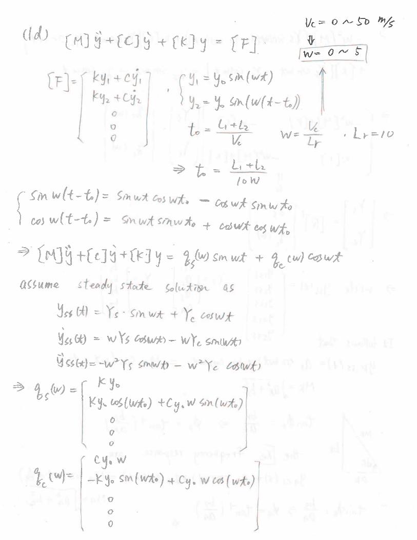
(1d) Consider a sinusoidal road surface of sinusoidal form

1 0 2 0 0( ) sin( ), ( ) sin( ( ))y t y t y t y t t

where c

r

v

L and 1 2

0

c

l lt

v

, with cv being the velocity of the car and rL being a characteristic

length describing the road condition. Assume that 0y = 0.08 m and rL = 10 m. Compute the

frequency response (both amplitude and phase) of the engine assembly ( ex ) versus the car speed

cv (from 0 m/s to 50 m/s).

Fall 2016


Task 2. A Model of Coupled Vehicle-Bridge Systems

A car moving on a bridge can be modeled as a moving rigid body coupled to a flexible beam

clamped at both ends; see Figs. 2 and 3. The rigid-body and beam are coupled by two pairs of

springs and viscous dampers that are a model of the tire-suspension assembly of the car.

Fig. 2

Fig. 3

(2a) Derive a mathematical model of the coupled vehicle-bridge system by the assumed-mode

method. To simplify your work, the following assumptions are made:

(A1) The effect of gravity on both the beam and rigid body is negligible.

(A2) At the initial time t = 0, the rear end of the car (the left end of the rigid body) coincides

with the left end of the bridge.

(A3) The car is moving rightward.

(A4) The model is only for the time period 0

0L a

tv

. In other words, during this time

period, all the tires of the car are within the bridge region ( 0 x L ).

Fall 2016


(2b) Let the parameters of the coupled system have the following values

Car: 3 2 2

5 31 2 1 2 0

4.5 m, 2.5 10 kg, 3.2 10 kg-m

5 10 / , 3.6 10 kg/s, 18 /

a M I

k k N m c c v m s

where M and I are the mass and moment of inertia of the car.

Bridge 2 8 28 10 kg/m, 7 10 , 400 mEI N m L

Consider three modes in the assumed-mode approximation of the beam. Let the beam is initially

at rest. Assume that the car has the following initial conditions:

1 1

2 1

(0) 0.02 , (0) 0.6 /

(0) 0.05 , (0) 0.3 /

y m y m s

y m y m s

Plot the displacements 1( )y t and 2 ( )y t of the car during the time period 0

0L a

tv

. Also, plot

the displacement of the beam versus the spatial coordinate x for 0 x L , at times t = j t ,

with j = 1,2,…, 6 and 06

L at

v

. Hint: refer to the class notes for numerical solutions.

(2c) Assume that the front tire of the car hits a rock in the middle of the bridge (x = L/2). The

collision between the rock and tire is modeled as an impulsive load

3

0

( ) ( ), with 1.2 10 kg m/s,2

o imp o imp

L af t I t t I t

v

that is applied to the rigid body at the front end where the spring/damper pair 2 2( , )k c is

connected. Assume that the car has the same initial conditions as given in (2b). Plot the

displacements 1( )y t and 2 ( )y t of the car during the time period 0

0L a

tv

. Compare the results

with those obtained in (2b) to see the influence of the tire-rock collision on the car vibration.

D1 =

-29.1170 +77.2601i

-29.1170 -77.2601i

-29.4529 +77.4448i

-29.4529 -77.4448i

-3.6197 +30.1922i

-3.6197 -30.1922i

-0.4719 +10.6523i

-0.4719 -10.6523i

-0.7196 +13.1701i

-0.7196 -13.1701i

vt1 =

Columns 1 through 5

-0.0033 - 0.0087i -0.0033 + 0.0087i 0.0028 + 0.0072i 0.0028 - 0.0072i 0.0003 + 0.0067i

-0.0028 - 0.0072i -0.0028 + 0.0072i -0.0033 - 0.0087i -0.0033 + 0.0087i -0.0001 - 0.0019i

0.0001 + 0.0004i 0.0001 - 0.0004i 0.0000 + 0.0000i 0.0000 - 0.0000i 0.0005 + 0.0043i

-0.0000 - 0.0000i -0.0000 + 0.0000i 0.0000 + 0.0001i 0.0000 - 0.0001i -0.0037 - 0.0311i

0.0000 + 0.0000i 0.0000 - 0.0000i -0.0001 - 0.0004i -0.0001 + 0.0004i 0.0007 + 0.0053i

0.7680 + 0.0000i 0.7680 + 0.0000i -0.6388 + 0.0057i -0.6388 - 0.0057i -0.2028 - 0.0142i

0.6393 - 0.0054i 0.6393 + 0.0054i 0.7684 + 0.0000i 0.7684 + 0.0000i 0.0565 + 0.0039i

-0.0356 - 0.0063i -0.0356 + 0.0063i -0.0025 - 0.0007i -0.0025 + 0.0007i -0.1329 + 0.0002i

0.0041 + 0.0005i 0.0041 - 0.0005i -0.0056 - 0.0006i -0.0056 + 0.0006i 0.9539 + 0.0000i

-0.0024 - 0.0005i -0.0024 + 0.0005i 0.0347 + 0.0061i 0.0347 - 0.0061i -0.1637 + 0.0003i

Columns 6 through 10

0.0003 - 0.0067i -0.0006 - 0.0299i -0.0006 + 0.0299i 0.0003 + 0.0057i 0.0003 - 0.0057i

-0.0001 + 0.0019i -0.0001 - 0.0045i -0.0001 + 0.0045i -0.0024 - 0.0447i -0.0024 + 0.0447i

0.0005 - 0.0043i -0.0016 - 0.0347i -0.0016 + 0.0347i -0.0031 - 0.0360i -0.0031 + 0.0360i

-0.0037 + 0.0311i -0.0035 - 0.0790i -0.0035 + 0.0790i 0.0028 + 0.0323i 0.0028 - 0.0323i

0.0007 - 0.0053i -0.0008 - 0.0185i -0.0008 + 0.0185i 0.0032 + 0.0362i 0.0032 - 0.0362i

-0.2028 + 0.0142i 0.3192 + 0.0081i 0.3192 - 0.0081i -0.0750 + 0.0002i -0.0750 - 0.0002i

0.0565 - 0.0039i 0.0484 + 0.0012i 0.0484 - 0.0012i 0.5905 + 0.0000i 0.5905 + 0.0000i

-0.1329 - 0.0002i 0.3707 - 0.0005i 0.3707 + 0.0005i 0.4766 - 0.0154i 0.4766 + 0.0154i

0.9539 + 0.0000i 0.8431 + 0.0000i 0.8431 + 0.0000i -0.4278 + 0.0139i -0.4278 - 0.0139i

-0.1637 - 0.0003i 0.1969 - 0.0002i 0.1969 + 0.0002i -0.4787 + 0.0159i -0.4787 - 0.0159i

D2 =

1.0e+03 *

0.1136

0.1738

0.9243

6.8234

6.8736

vt2 =

-0.0148 0.0024 0.0121 -0.0876 -0.0728

-0.0022 -0.0189 -0.0034 -0.0731 0.0873

-0.0172 -0.0153 0.0080 0.0038 -0.0003

-0.0390 0.0137 -0.0574 -0.0004 -0.0006

-0.0091 0.0154 0.0098 0.0003 0.0037

[vt2]’*[M]*[vt2]=

1.0000 -0.0000 0.0000 -0.0000 0.0000

-0.0000 1.0000 -0.0000 -0.0000 0.0000

0.0000 -0.0000 1.0000 0.0000 -0.0000

-0.0000 -0.0000 0.0000 1.0000 0.0000

0.0000 0.0000 -0.0000 0.0000 1.0000

[vt2]’*[K]*[vt2]=

1.0e+03 *

0.1136 0.0000 -0.0000 0.0000 -0.0000

0.0000 0.1738 0.0000 0.0000 0.0000

-0.0000 0.0000 0.9243 0.0000 -0.0000

0.0000 0.0000 0.0000 6.8234 0.0000

-0.0000 0.0000 -0.0000 0.0000 6.8736

0 0.5 1 1.5 2 2.5 3 3.5 4 4.5 50.08

0.085

0.09

0.095

0.1

0.105

0.11Amplitude

w (rad/s)

Am

plit

ude (

m)

0 0.5 1 1.5 2 2.5 3 3.5 4 4.5 50.01

0.015

0.02

0.025

0.03

0.035Phase

w (rad/s)

ata

n

%AME 521 Project Task1 Kengyu Lin USCID:9852103390 clear; clc;

%~1a me=200; %kg k2=1.3*10^5; %N/m c2=1.02*10^3; %kg/s d=1.65; %m Mb=1650; %kg Ib=2330; %kg-m^2 k1=2.5*10^5; %N/m c1=2.73*10^3; %kg/s m=75; %kg k=2.5*10^5; %N/m c=1.48*10^3; %kg/s L1=1.4; %m L2=1.3; %m syms w Lr=10; %m vc=Lr*w; %m/s~~~~~~varible t0=(L1+L2)/vc; y0=0.08; %m

M=[m 0 0 0 0; 0 m 0 0 0; 0 0 Mb 0 0; 0 0 0 me 0; 0 0 0 0 Ib]; C=[c1+c 0 -c1 0 -c1*L2; 0 c1+c -c1 0 c1*L1; -c1 -c1 2*c1+c2 -c2 c1*L2-c1*L1+c2*d; 0 0 -c2 c2 -c2*d; -c1*L2 c1*L1 c2*d+c1*L2-c1*L1 -c2*d c2*d^2+c1*L2^2+c1*L1^2]; K=[k1+k 0 -k1 0 -k1*L2; 0 k1+k -k1 0 k1*L1; -k1 -k1 k2+2*k1 -k2 k2*d+k1*L2-k1*L1; 0 0 -k2 k2 -k2*d; -k1*L2 k1*L1 k2*d+k1*L2-k1*L1 -k2*d k2*d^2+k1*L2^2+k1*L1^2];

%~1b AZ=[zeros(5) eye(5);-inv(M)*K -inv(M)*C]; [vt1,D1]=eig(AZ); % with damp D1=eig(AZ) vt1

%~1c [vt2,D2]=eig(K,M); %undamp D2=eig(K,M) vt2 % check orthogonal vt2'*M*vt2 vt2'*K*vt2

%~1d qs=[k*y0; k*y0*cos(w*t0)+c*y0*w*sin(w*t0) ;0;0;0];

qc=[c*y0*w; -k*y0*sin(w*t0)+c*y0*w*cos(w*t0) ;0;0;0];

Q=[-w^2*[M]+[K] -w*[C];w*[C] -w^2*[M]+[K]]; qq=[qs;qc]; YY=inv(Q)*qq; a4=YY(4,:); b4=YY(9,:);

figure(1) subplot(2,1,1) M4=(a4^2+b4^2)^0.5; for ww=0:0.01:5 M4ww=subs(M4,ww); plot(ww,M4ww) hold on grid on end title('Amplitude') xlabel('w (rad/s)') ylabel('Amplitude (m)')

subplot(2,1,2) fi=atan(b4/a4); for ww=0:0.01:5 fiww=subs(fi,ww); plot(ww,fiww) hold on grid on end title('Phase') xlabel('w (rad/s)') ylabel('atan')

0 5 10 15 20 25-0.03

-0.02

-0.01

0

0.01

0.02

0.03

0.04y1 displacement

time (s)

magnitude (

m)

0 5 10 15 20 25-0.04

-0.02

0

0.02

0.04

0.06y2 displacement

time (s)

magnitude (

m)

0 100 200 300 400-15

-10

-5

0

5x 10

-6 beam displacement 1*dt

beam long (m)

magnitude (

m)

0 100 200 300 400-4

-2

0

2x 10


beam long (m)m

agnitude (

m)

0 100 200 300 400-3

-2

-1

0x 10


beam long (m)

magnitude (

m)

0 100 200 300 400-6

-4

-2

0

2x 10


beam long (m)

magnitude (

m)

0 100 200 300 400-3

-2

-1

0x 10


beam long (m)

magnitude (

m)

0 100 200 300 400-2

-1

0

1x 10


beam long (m)

magnitude (

m)

0 5 10 15 20 25-0.03

-0.02

-0.01

0

0.01

0.02

0.03

0.04y1 displacement

time (s)

magnitude (

m)

0 5 10 15 20 25-0.04

-0.02

0

0.02

0.04

0.06y2 displacement

time (s)

magnitude (

m)

%%AME 521 Project Task2 Kengyu Lin USCID:9852103390 clear; clc;

a=4.5; m=2.5*10^3; I=3.2*10^2; k1=5*10^5; k2=5*10^5; c1=3.6*10^3; c2=3.6*10^3; V0=18; p=8*10^2; EI=7*10^8; L=400;

%===== Ma Mb=zeros(3); for i=1:1:3 for j=1:1:3 Mbfun = @(x) p.*(1-cos(2.*i.*pi.*x./L)).*(1-cos(2.*j.*pi.*x./L)); Mb(i,j) = integral(Mbfun,0,L); end end Mbb=[m/4+I/(a^2) m/4-I/(a^2);m/4-I/(a^2) m/4+I/(a^2)]; Ma=[[Mb] zeros(3,2);zeros(2,3) [Mbb]]; %===== Kb Kb=zeros(3); for i=1:1:3 for j=1:1:3 Kbfun = @(x)

EI.*((2.*i.*pi./L).^2*cos(2.*i.*pi.*x./L)).*((2.*j.*pi./L).^2.*cos(2.*j.*pi.*

x./L)); Kb(i,j) = integral(Kbfun,0,L); end end

% Ca Ka are martix function of t, so I put both in the AZ.m for doing the % numerical solution

Z0=[0 0 0 0.02 0.05 0 0 0 0.6 -0.3]'; N=3000; % choose this number can be divide by 6, in order to find dt for

finding beam's displacement tend=(L-a)/V0; h=(L-a)/(V0*N); z=Z0; Z(:,1)=Z0; k=1; T(:,1)=0; for t=0:h:tend %Runge-Kutta Method f1=AZ(t,z,Ma,Kb); f2=AZ(t+h/2,z+h/2*f1,Ma,Kb); f3=AZ(t+h/2,z+h/2*f2,Ma,Kb); f4=AZ(t+h,z+h*f3,Ma,Kb);

Z(:,k+1)=Z(:,k)+(h/6)*(f1+2*f2+2*f3+f4);

z=Z(:,k+1); T(1,k+1)=t; k=k+1; end

figure(1) subplot(2,1,1) plot(T,Z(4,:),'r') title('y1 displacement') xlabel('time (s)') ylabel('magnitude (m)') grid on

subplot(2,1,2) plot(T,Z(5,:),'b') title('y2 displacement') xlabel('time (s)') ylabel('magnitude (m)') grid on

%=======beam dispacement

k=1; for i=1:500:3001 for dx=1:1:400 Wb(k,dx)=admfun(dx)*Z(1:3,i); end k=k+1; end dx=1:1:400;

figure(2) subplot(3,2,1) plot(dx,Wb(2,:)) title('beam displacement 1*dt') xlabel('beam long (m)') ylabel('magnitude (m)') grid on

subplot(3,2,2) plot(dx,Wb(3,:)) title('beam displacement 2*dt') xlabel('beam long (m)') ylabel('magnitude (m)') grid on


subplot(3,2,4) plot(dx,Wb(5,:))

title('beam displacement 4*dt') xlabel('beam long (m)') ylabel('magnitude (m)') grid on



%========y1 y2 impulsive load

addyy2=1.2/2.5; for t=0:h:tend %Runge-Kutta Method f1=AZ(t,z,Ma,Kb); f2=AZ(t+h/2,z+h/2*f1,Ma,Kb); f3=AZ(t+h/2,z+h/2*f2,Ma,Kb); f4=AZ(t+h,z+h*f3,Ma,Kb); Z(:,k+1)=Z(:,k)+(h/6)*(f1+2*f2+2*f3+f4);

if k==1500 %add impulsive load on y2' at x=L/2 Z(10,k+1)=Z(10,k+1)+addyy2; end

z=Z(:,k+1); T(1,k+1)=t; k=k+1; end

figure(3) subplot(2,1,1) plot(T,Z(4,:),'r') title('y1 displacement') xlabel('time (s)') ylabel('magnitude (m)') grid on

subplot(2,1,2) plot(T,Z(5,:),'b') title('y2 displacement') xlabel('time (s)') ylabel('magnitude (m)') grid on

References

[1] B. Yang, AME 521 Lecture Notes 2016.

[2] B. Yang, AME 521 homework solution 11 & 12.

[3] H. P. Gavin, "Numerical integration in structural dynamics," 2016. [Online].

Available: http://people.duke.edu/~hpgavin/cee541/NumericalIntegration.pdf.

Accessed: Dec. 5, 2016.

[4] "Appendix A numerical integration methods,". [Online]. Available:

https://theses.lib.vt.edu/theses/available/etd-10052004-

201201/unrestricted/07_Appendix.pdf. Accessed: Dec. 5, 2016.

Documents

Task 1. A Five-DOF Model of Automobiles Task 2. Model of … · 2018-09-07 · This project consists of two tasks on modeling and analysis of vibrating systems: Task 1. A Five-DOF