Taper equations based on nonlinear mixed effect … · de datos de validación, el esquema de muestreo con tres submuestra de diámetro superior en un árbol produjo los mejores resultados

BOSQUE 38(3): 545-554, 2017 DOI: 10.4067/S0717-92002017000300012

545

Taper equations based on nonlinear mixed effect modeling approach for Pinus nigra in Çankırı forests

Ecuaciones de ahusamiento basadas en un enfoque de modelado no lineal de efectos mixtos para Pinus nigra en bosques de Çankırı

Muammer Şenyurt a*, İlker Ercanlı, a, Ferhat Bolat a

* Corresponding author: a Çankırı Karatekin University, Faculty of Forestry, Department of Forest Engineering, Çankırı, Turkey, phone +90-3762122757, [email protected]

SUMMARY

In this study, statistical nonlinear mixed effect models were used to model taper of individual trees in Pinus nigra stands distributed within the Çankırı Forests. The data from 210 trees that were felled from Pinus nigra stands were used in this study. Three tree taper equations were fitted and evaluated based on the sum square error (SSE), mean square error (MSE), root mean square error (RMSE) and the adjusted coefficient of determination (R2

adj). The Jiang et al.’s equation was found to produce the most satisfactory fits with the SSE (4125.7), MSE (2.1771), RMSE (1.4755) and (0.976). The stem taper equation of Jiang et al. was used within the scope of mixed-effect model structures that involved both random and constant effect parameters. The nonlinear mixed-effect modeling approach for the stem taper equation of Jiang et al. with SSE (3254.8), MSE (1.71759), RMSE (1.3119) provided much better fitting and precise predictions than those produced by the nonlinear fixed effect model structures for this model. Within various sampling scenarios including different numbers of the sub-sample trees based on some sampling strategies from the validation data set, the sampling scheme with three top diameter sub-sample in a tree produced the best predictive results (SSE = 313.5321, MSE = 0.8637 and RMSE = 0.9345) in relation to the fixed effect predictions.

Key words: diameter, estimate, random parameters, segmented polynomial model.

RESUMEN

En este estudio se utilizaron modelos estadísticos no lineales de efectos mixtos para modelar el ahusamiento de árboles individuales en rodales de Pinus nigra distribuidos en bosques de Çankırı. Se utilizaron datos de 210 árboles que fueron talados. Se ajustaron y evaluaron tres ecuaciones de ahusamiento de árbol, basadas en la suma del error cuadrático (SSE), el error cuadrático medio (MSE), la raíz del error cuadrático medio (RMSE) y el coeficiente de determinación ajustado (R2adj). La ecuación de Jiang et al. produjo los ajustes más satisfactorios según SSE (4125,7), MSE (2,1771), RMSE (1,4755) y Radj2(0,976). Esta ecuación de ahusamiento del fuste se utilizó en el ámbito de un modelo de efecto mixto que involucra parámetros del azar y del efecto constante. El modelo no lineal de efectos mixtos para la ecuación de ahusamiento del fuste de Jiang et al. con SSE (3.254,8), MSE (1,71759) y RMSE (1,3119), proporcionó predicciones más ajustadas y precisas que los modelos no lineales de efectos fijos. Dentro de varios escenarios de muestreo, incluyendo diferentes números de los árboles de submuestra, basados en algunas estrategias de muestreo del conjunto de datos de validación, el esquema de muestreo con tres submuestra de diámetro superior en un árbol produjo los mejores resultados predictivos (SSE = 313,5321, MSE = 0,8637 y RMSE = 0,9345) en relación con las predicciones de efecto fijo.

Palabras clave: diámetro, estimación, parámetros aleatorios, modelo polinomial segmentado.

INTRODUCTION

Stem taper equations are used to estimate in detail the volume of a single tree between the ground level and a cer-tain height on the stem, or between two different heights on the stem of a tree (Yavuz 1995, Özçelik et al. 2012). In this context, in order to accurately determine in detail the volume of wood that can be obtained from individual trees, there is a need to develop stem taper equations for every type of tree and forest site.

Max and Burkhart (1976) developed a stem taper mo-del, named the Segmented Polynomial Stem Profile Mo-del, in which a different polynomial is formed for every segment of the tree that exhibits a different form (rather than a single polynomial for the entire stem), and the poly-nomials are subsequently combined within a single model. This model, which has been revealed as statistically relati-vely accurate, has been extensively used by many resear-chers to estimate the stem taper of different types of trees (Demaerschalk and Kozak 1977, Czaplewski and Mcclure

BOSQUE 38(3): 545-554, 2017Taper equations based on nonlinear mixed effect

546

1988). As different from the equation of Max and Burkhart (1976), Parresol et al. (1987) presented a power equation connecting and combing two cubic polynomials. Jiang et al. (2005) improved Max and Burkhart (1976) equation by adding upper diameter, e.g. upper diameter values at 5.30 m, and also found that the addition of this upper diameter as a predictor variable provided modest improvements.

Stem taper equations generally use taper data obtained at different heights from each individual tree, and form a data pool consisting of statistics collected through multiple measurements of trees with different stem growth sites. In these hierarchal data structures, where every tree exhibits its own specific type of stem growth, researchers often en-counter the problem known as “serial-correlation or auto-correlation”, a situation where a certain level of dependen-ce is observed among different data (Leites and Robinson 2004). Such correlations among sample data may lead to systematic errors in confidence interval estimations during the calculation of stem taper and stem volume equation parameters, which in turn can negatively affect the relia-bility of the model results (Searle et al. 1992). In this res-pect, when dealing with hierarchal data structures where the condition of data independence is not met, there is an issue of autocorrelation problem among data; the linear and non-linear mixed effect models that enable the mode-ling of variance-covariance matrices are usually utilized instead of prediction models based on the use of ordinary least squares (OLS) for linear models or nonlinear least squares (NLS) technique for nonlinear models (Littell et al. 2005).

Pinus nigra Arnold. subsp. pallasiana (Lamb.) Holm-boe is one of the most economically and ecologically im-portant forest tree species for Turkey with valuable wood for many commercial uses. Pinus nigra prefers full sun, moist to dry conditions that are well-drained, and acidic sandy soil, although it also adapts to other kinds of soil. Pinus nigra often forms forests of pure or mixed type, in higher mountainous areas of Anatolia; however, it also extends to inner and other regions in the form of small patches. Pinus nigra grows naturally in Turkey and is lo-cated in the Marmara, Aegean and Mediterranean regions, as well as in many other regions of the world (Davis 1982). In Turkey, Pinus nigra covers 4,244,921 ha and composes nearly 19 % of the country’s total forest area (General Di-rectorate of Forestry 2015). Pinus nigra stands with diffe-rent forest structures and bio-diversity are widespread in the forest areas of Turkey. The management of these stands of this species is of increasing importance to foresters in Turkey, and a crucial factor is knowledge of tree taper esti-mation for the sound management of these stands. Despite the importance of Pinus nigra species in this region, only a few studies concerning the taper prediction systems based on nonlinear mixed effect models exist. Thus, the objecti-ves of the present study is (1) to compare some Nonlinear Segmented Polynomial Stem Taper Equations to predict tree taper of Pinus nigra trees distributed in the Çankırı

Forests, (2) to apply the nonlinear mixed effect modeling approach was applied to the best predictive equation by predicting the parameters and variance components of this equation and (3) to evaluate some calibration strategies including different numbers of sub-sample trees to speci-fying sampling unit-specific effect into the taper predic-tions.

METHODS

The study was performed using data from 210 trees that were felled in the Pinus nigra stands of the Çankırı Fo-rests within the Çankırı Forest Management Directorate (Şenyurt et. al. 2014). The sample trees were randomly selected to represent various tree diameter and height sizes with the best variability in volume development. Attention was specifically paid to ensuring that none of the collected sample trees had damaged tips, damaged wood (broken tips or cracked and dried wood), insect-related damage, fungus-related damage or injuries (caused by whichever reason) that led to stem rot.

Within the scope of this study, sample trees were felled at the height of 0.3 m (the base of the trunk); the stem diameter over bark (cm) was first measured at this height. Following this, measurements were continued at regular intervals of one meter by using a steel measuring tape, hence measurements were taken at 1.3 m, 2.3 m, 3.3 m, etc. In addition, the total height of trees was also measured with a steel measuring tape. Thus, a total of 2,462 taper/diameter measurements were obtained from the 210 sam-ple trees used in this study. Table 1 provides the summary statistics, such as the mean, standard deviations, minimum and maximum of diameter at breast height (dbh) and total height (h) for model fitting and validation data set.

The data used within the scope of the study were ran-domly divided into two groups: modeling data used for estimating the parameters of the equations, and validation data used for assessing the suitability of the functions for the studied stands. Nearly 85 % (n = 178) of the trees were in the former group (Group I), while 15 % (n = 32) of the trees were in the latter group (Group II).

Table 1. Summary statistics for sample trees originated from fit-ting and validation data. Resumen de estadísticas de los árboles de muestra originadas de datos de ajuste y validación.

Type of data Variables Min. Max. Mean Standard deviation

Fitting datadbh (cm) 4.0 48.6 22.5 9.4

h (m) 3.75 16.3 11.7 2.0

Validation datadbh (cm) 5.2 44.0 24.1 10.3

h (m) 4.3 17.0 11.5 2.7


547

Taper equations. While early stem taper equations attemp-ted to represent the change in diameter/taper across the stem with a single equation, Max and Burkhart (1976) de-veloped a different stem taper model, named the segmen-ted polynomial stem profile model [equation 1], in which a different polynomial is formed for every segment of the tree that exhibits a different form, and the polynomials are subsequently combined within a single model.

[1]

Where, d: stem diameter over bark (cm) at a height h (m), dbh: diameter at breast height over bark (cm), h: measuring height (m), H: total height (m), a1 and a2 are join points in-cluding conic, parabolic and nayloid stem forms for the data.

With a transformation based on the Max and Burkhart (1976) equation, Parresol et al. (1987) developed the equa-tion shown below [equation 2]:

[2]

Clark et al. (1991) later developed a segmented poly-nomial stem profile model that differs from the model de-veloped by Max and Burkhart (1976); Jiang et al. (2005), on the other hand, used the segmented polynomial stem profile equation proposed by Clark et al. (1991) as a basis to develop a new equation consisting of fewer parame-ters. This equation, as developed by Jiang et al. (2005), is shown below [equation 3].

[3]

Where d5.3: stem diameter over bark (cm) at 5.3 meters of stem height.

In this study, a number of different statistical criteria were used to determine the most successful of these three different stem taper models. These criteria included the sum square error (SSE), mean square error (MSE), root mean square error (RMSE), Akaike’s information criterion (AIC), Schwarz’s Bayesian Information Criterion (BIC) and the adjusted coefficient of determination (R2

adj). With these criteria, it is desirable for the SSE, MSE, RMSE, AIC and BIC to have as small value as possible, while the R2

adj is expected as close as possible to 1. The formulae for

d2

dbh2 = b1(z − 1) + b2(z2 − 1) + b3(a1 − z)2 I1 + b4(a2 − z)2 I2 [1]

z = hH Ii = {1 z ≤ ai

0 z > ai i = 1, 2}

d2

dbh2 = 𝑡𝑡(b1 − b2t) + (t − a)2(b3 + b4(t + 2a))I [2]

I = {1 𝑡𝑡 ≤ a0 t > a } t = (H − h) H⁄

d =

{

IS [dbh2 (1 +

(1−𝑧𝑧)b1−(1−1.30 H⁄ )b1)1− (1−1.30 H⁄ )b1 )]

+ IB [dbh2 − (dbh2− d5.32 )((1−1.30 H⁄ )b2− (1−𝑧𝑧)b2)

(1−1.30 H⁄ )b2− (1−5.30 H⁄ )b2 ] +

+ IT [(𝑑𝑑5.3)2 (b4 (h−5.30H−5.30 − 1)

2+ IM (

1−b4b32) (b3 −

h−5.30H−5.30)

2)]}

0.5

[3]

these statistical values are provided below ([equation 4] to [equation 9]).

[4]

[5]

[6]

[7]

[8]

[9]

Where: di represents stem diameter over bark (cm) at a height h (m); represents the estimated diameter value with the developed stem taper model, represents average diameter, n represents the number of data, L means Maxi-mum value of the log likelihood function and p represents the number of parameters within the model.

The PROC MODEL procedure from the SAS Statisti-cal Package Software (SAS Institute Inc. 2013) was used both for estimating the parameters of the stem taper equa-tions listed above and for determining the various statisti-cal criteria for success.

Nonlinear mixed effect modeling approach. The parame-ters and variance components of the equation that was de-termined to be the most effective among the three stem taper equations were estimated with the Nonlinear Mixed Effect Modeling Technique. In mixed models, the fact that model parameters are classified as fixed effect and random effect parameters is shown as follows [equation 10]:

[10]

Here, β is the parameter associated with fixed effects, and is calculated for the entire population, while bi is the parameter associated with the random effects, and differs among sample trees (Castedo Dorado et al. 2006, Cre-cente-Campo et al. 2010). In mixed models, the basic as-sumption for the model errors and the parameters for the random effects are shown as follows:

Mean squared errors (MSE) = ∑ (di di)2

n pni = 1

Root mean squared error (RMSE) = √∑ (di − d��𝑖)2

n − p

n

i = 1

Sum of Squared error (SSE) = ∑(di − di)2

n

i = 1

Adjusted cofficient of determination (Radj.2 ) = 1 −

∑ (di − di)2n

i = 1 (n − 1)∑ (di − di)

2ni = 1 (n − p)

Adjusted cofficient of determination (Radj.2 ) = 1 −

∑ (di − di)2n

i = 1 (n − 1)∑ (di − di)

2ni = 1 (n − p)

𝐴𝐴𝐴𝐴𝐴𝐴 = −2𝑙𝑙𝑙𝑙𝑙𝑙𝑙𝑙 + 2𝑝𝑝

𝐵𝐵𝐵𝐵𝐵𝐵 = −2𝑙𝑙𝑙𝑙𝑙𝑙(𝐿𝐿) + 𝑝𝑝𝑙𝑙𝑙𝑙𝑙𝑙(𝑁𝑁)

Φi = Aijβ + Bijbi

𝑑𝑑��𝑖 di


548

[11]

[12]

Where bi is the arithmetic mean of the parameter for ran-dom effects, and is 0 with a variance of D; εij, the model error, has an arithmetic mean of 0 and a variance of R, and has a normal distribution (Calama and Montero 2004, Castedo Dorado et al. 2006). The estimations for matrices D and R that is expressed in these assumptions are an im-portant aspect of mixed models (Lappi 1997). The matrix is a positive variance-covariance matrix that describes the variability among the tree samples (inter-tree variability), while the R matrix is a variance-covariance matrix that describes variability among the measured data on a given tree sample (intra-tree variability). The formulae for the D and R variance-covariance matrices, which define and model the variability between both the sample trees and the measured data, are shown in the equations below:

[13]

[14]

In the equations [equation 13] and [equation 14], σ2u σ

2v

represents the variance of the random effect parameter u, represents the variance of the random effect v, σ2

uv repre-sents the covariance among the random effect parameters, represents the error value for the model, and Ii represents the diagonal matrix value with the non-fixed variance and which dimension of matrix is equal to the number of data used for the sub-sample trees (Castedo Dorado et al. 2006, Trincado et al. 2007).

In this study, the predictions for variance components and fixed parameters of the taper equation selected as best predictive were obtained by PROC NLMIXED procedures of the SAS/ETS V9 software (SAS Institute Inc. 2013). In a nonlinear mixed effect regression, SAS PROC NL-MIXED uses the maximum likelihood estimation (ML) procedure. The adaptive Gaussian quadrature was used to solve numerically the integral over the random effects in SAS NLMIXED procedure. Pinheiro and Bates (2000) presented the detailed information for this procedure.

Calibration response. For the application of the Mixed Effect Modeling on different growing environments and stands, the random effect parameters will be estimated based on the new data set obtained from the other forest areas. This subsequent process following the estimation of the fixed effect parameters within the equation along with the variance components relating to these parameters have been called as “calibrating mixed effect models”.

When calibrating the mixed effect modeling to a particu-lar area, a number of diameter values measured on sample

Φi = Aijβ + Bijbi

ℇij~N(0, R)

D = [ σu2 σuv

2

σuv2 σv

2 ]

R = σ2Ii

trees collected from the other forest area are first used to calculate the random parameters; after this, a random effect parameter is added to (or, if it is a negative value, subtrac-ted from) this calculated fixed effect parameter value that is valid for the entire population. In forestry applications, the calibration of mixed models is performed according to the Best Linear Unbiased Predictor (BLUP) formula first used by Lappi (1991), and which is also designated as the Hender-son equations. In their studies, Calama and Montero (2004), Trincado and Burkhart (2006), Lejeune et al. (2009), Shar-ma and Parton (2009), Yang et al. (2009), and Özçelik et al. (2011) used BLUP equations for estimating random effect parameters. In this study, 32 different tree data selected for model calibration with the method described above were used for determining the calibration response of the mixed models. In the application of the BLUP formula and the cal-culation of the random parameters, the SAS program code provided by Trincado et al. (2007) was employed. In this study, to determine the calibration response of the mixed effect nonlinear stem taper model, comparisons were made among four different calibration response options, involving the use of diameter values measured at different heights of trees. The calibration response options in question were:

1.) Three diameters from the lowest base section of the sample tree,

2.) Three diameters that divide the sample tree measu-rements into two equal parts,

3.) Three diameters that are closest to the top of the sample tree,

4.) Three diameter values obtained respectively from the base, midsection and top of the sample tree.

These diameter values were afterward used to calcu-late the random parameters for these sample trees with the SAS program source code provided by Trincado et al. (2007). For these sample trees, the diameter values were estimated with this calibrated stem taper equation by using random parameters based on different calibration response options. The success of the model estimations was subse-quently calculated based on the differences between the estimated and observed diameter values, according to the SSE, MSE and RMSE criteria.

RESULTS

Taper equations. The parameter estimations, standard error values, t-values and their significance levels for the three -- Max and Burkhart (1976), Parresol et al. (1987) and Jiang et al. (2005)-- equations with the success criteria for the different models used in this study are all shown in table 2. All parameters for these equations were determined to be statistically significant with P value < 0.05.

The success criteria of the Max and Burkhart (1976) equation were MSE: 3.2913, RMSE: 1.8168, SSE: 6892.01 and R2

adj: 0.956, while those for the Parresol et al. (1987)

549


equation were MSE: 3.6649, RMSE: 1.9162, SSE: 7674.3, R2

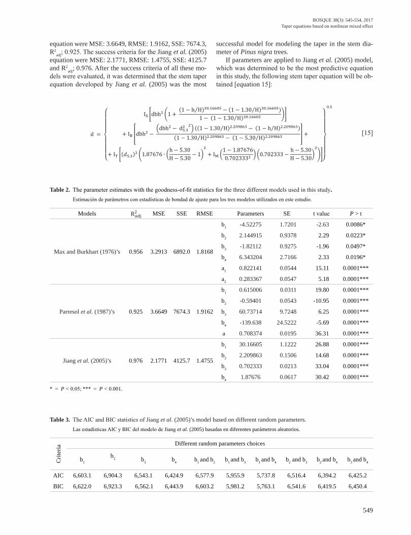
adj; 0.925. The success criteria for the Jiang et al. (2005) equation were MSE: 2.1771, RMSE: 1.4755, SSE: 4125.7 and R2

adj; 0.976. After the success criteria of all these mo-dels were evaluated, it was determined that the stem taper equation developed by Jiang et al. (2005) was the most

d =

{

IS [dbh2 (1 +

(1 − h H⁄ )30.16605 − (1 − 1.30 H⁄ )30.16605)1 − (1 − 1.30 H⁄ )30.16605 )]

+ IB [dbh2 − (dbh2 − d5.32

2) ((1 − 1.30 H⁄ )2.209863 − (1 − h H⁄ )2.209863)(1 − 1.30 H⁄ )2.209863 − (1 − 5.30 H⁄ )2.209863 ] +

+ IT [(𝑑𝑑5.3)2 (1.87676 ∙ (h − 5.30H − 5.30 − 1)

2+ IM (

1 − 1.876760.7023332 ) (0.702333 −

h − 5.30H − 5.30)

2)]}

0.5

successful model for modeling the taper in the stem dia-meter of Pinus nigra trees.

If parameters are applied to Jiang et al. (2005) model, which was determined to be the most predictive equation in this study, the following stem taper equation will be ob-tained [equation 15]:

[15]

Table 2. The parameter estimates with the goodness-of-fit statistics for the three different models used in this study. Estimación de parámetros con estadísticas de bondad de ajuste para los tres modelos utilizados en este estudio.

Models MSE SSE RMSE Parameters SE t value P > t

Max and Burkhart (1976)’s 0.956 3.2913 6892.0 1.8168

b1 -4.52275 1.7201 -2.63 0.0086*

b2 2.144915 0.9378 2.29 0.0223*

b3 -1.82112 0.9275 -1.96 0.0497*

b4 6.343204 2.7166 2.33 0.0196*

a1 0.822141 0.0544 15.11 0.0001***

a2 0.283367 0.0547 5.18 0.0001***

Parresol et al. (1987)’s 0.925 3.6649 7674.3 1.9162

b1 0.615006 0.0311 19.80 0.0001***

b2 -0.59401 0.0543 -10.95 0.0001***

b3 60.73714 9.7248 6.25 0.0001***

b4 -139.638 24.5222 -5.69 0.0001***

a 0.708374 0.0195 36.31 0.0001***

Jiang et al. (2005)’s 0.976 2.1771 4125.7 1.4755

b1 30.16605 1.1222 26.88 0.0001***

b2 2.209863 0.1506 14.68 0.0001***

b3 0.702333 0.0213 33.04 0.0001***

b4 1.87676 0.0617 30.42 0.0001***

* = P < 0.05; *** = P < 0.001.

Table 3. The AIC and BIC statistics of Jiang et al. (2005)’s model based on different random parameters. Las estadísticas AIC y BIC del modelo de Jiang et al. (2005) basadas en diferentes parámetros aleatorios.

Crit

eria Different random parameters choices

b1 b2 b3 b4 b1 and b2 b1 and b3 b1 and b4 b2 and b3 b2 and b4 b3 and b4

AIC 6,603.1 6,904.3 6,543.1 6,424.9 6,577.9 5,955.9 5,737.8 6,516.4 6,394.2 6,425.2

BIC 6,622.0 6,923.3 6,562.1 6,443.9 6,603.2 5,981.2 5,763.1 6,541.6 6,419.5 6,450.4

Radj2

ments that will be performed for the BLUP formula. By using the variance values of random effect parameters and the covariance values between the two parameters asso-ciated with Nonlinear Mixed Effect Model, the D matrix is obtained as follows [equation 17]:

[17]

In this matrix, the variance value of b1 parameter is 666.94, the variance value of b4 parameter is 0.4596, and the value of the covariance between the two parameters is 1.4089. The R matrix was obtained as follows [18]:

[18]

In this matrix, the equation error is 0.8300, while is the value of the 3x3 diagonal matrix (the number of data selected for calibration in the sample trees on which the mixed model will be employed).

The estimated SSE, MSE, and RMSE values based on these sample trees are shown in table 5. Among these ca-libration choices, the best results were obtained with the choice involving the measurement of three diameters that are closest to the top of the sample tree. This option was fo-llowed in terms of success by the calibration response choi-ce involving three diameter values obtained by dividing the measured diameters into two equal parts; the calibration

[16]


550

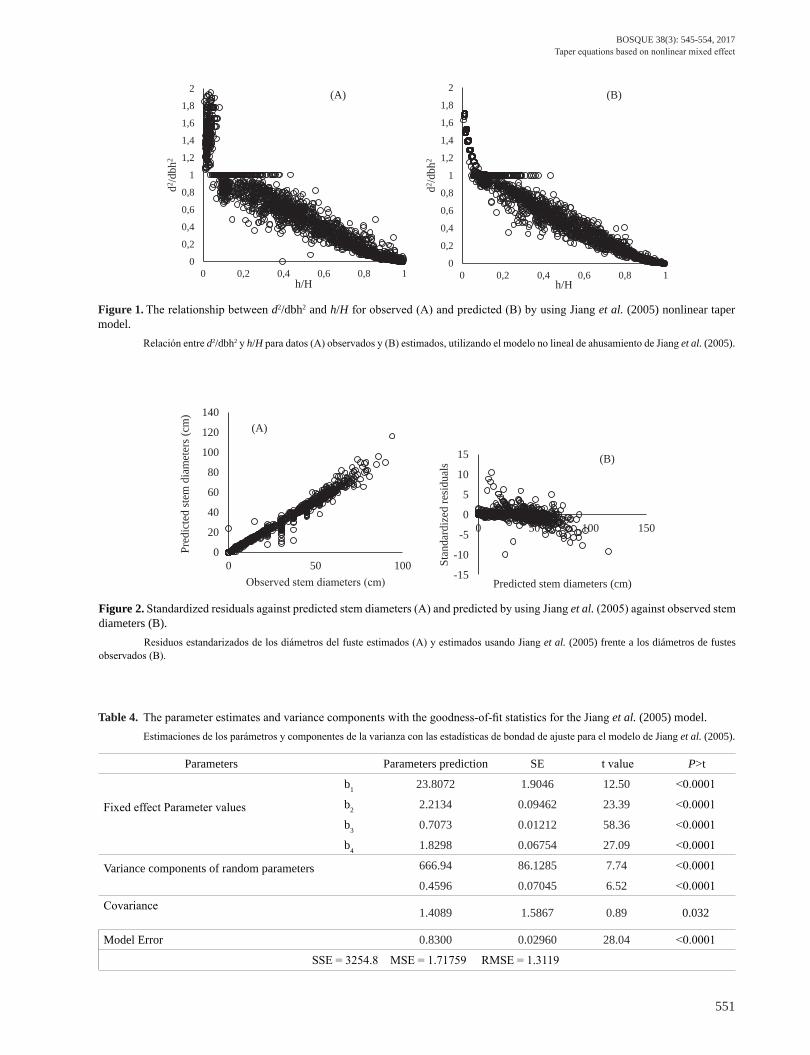
The relationship between d 2/dbh

2 and h/H for observed and predicted by using Jiang et al. (2005) nonlinear ta-per model is shown in figure 1. In addition, the residuals against predicted diameters (a) and predicted diameters against observed diameters (b) for Jiang et al. (2005) non-linear taper model are shown in figure 2.

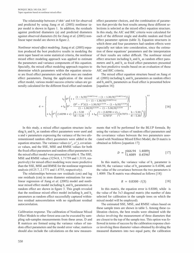
Nonlinear mixed effect modeling. Jiang et al. (2005) equa-tion produced the best predictive results in modeling the stem taper based on some statistical criteria, the nonlinear mixed effect modeling approach was applied to estimate the parameters and variance components of this equation. Specially, the mixed effect modeling approach requires to determine which parameters within the equation structu-re are fixed effect parameters and which ones are random effect parameters. During the application of the mixed effect model, various model success criteria values are ge-nerally calculated for the different fixed effect and random

effect parameter choices, and the combination of parame-ters that provide the best results among these different se-lections is selected as the mixed effect equation structure. In this study, the AIC and BIC criteria were calculated for each of the different single and double random and fixed effect parameter options (table 3). Equation structures in which three and four parameters had random effects were especially not taken into consideration, since the estima-tion of these equations’ parameters and the interpretation of their results are rather difficult. The nonlinear mixed effect structure including b1 and b4 as random effect para-meters and b2 and b3 as fixed effect parameters presented the best predictive results based on an evaluation of these AIC and BIC criteria.

The mixed effect equation structure based on Jiang et al. (2005) including b1 and b4 parameters as random effect and b2 and b3 parameters as fixed effect is presented below [equation 16]:

d =

{

IS [D2 (1 +

(1 − h H⁄ )(23.8072+u) − (1 − 1.30 H⁄ )(23.8072+u))1 − (1 − 1.30 H⁄ )(23.8072+u) )]

+ IB [D2 − (D2 − F2)((1 − 1.30 H⁄ )2.2134 − (1 − h H⁄ )2.2134)

(1 − 1.30 H⁄ )2.2134 − (1 − 5.30 H⁄ )2.2134 ] +

+ IT [F2 ((1.8298 + v) ∙ (h − 5.30H − 5.30 − 1)

2+ IM (

1 − (1.8298 + v)0.70732 ) (0.7073 − h − 5.30

H − 5.30)2)]}

0.5

𝐷𝐷 = [666.94 1.40891.4089 0.4596]

𝑅𝑅 = 0.8300 ∙ 𝐼𝐼(3)

In this study, a mixed effect equation structure inclu-ding b1 and b4 as random effect parameters were used and u and v parameters expressing the variance of the two afo-rementioned random effect parameters were added to the equation structure. The variance values (σ2

u, σ2u), covarian-

ce values, and the SSE, MSE and RMSE values for both the fixed effect parameters and random effect parameters in the mixed effect model were presented in table 4. The SSE, MSE and RMSE values (3254.8, 1.71759 and 1.3119, res-pectively) for mixed effect modeling were more predictive than the SSE, MSE and RMSE for the nonlinear regression analysis (4125.7, 2.1771 and 1.4755, respectively).

The relationships between raw residuals (cm) and lag one residuals (cm) in stem diameter estimations for non-linear regression of Jiang et al. (2005) model and nonli-near mixed effect model including b1 and b4 parameters as random effect are shown in figure 3. This graph revealed that the nonlinear mixed effect model including b1 and b4 parameters as random effect successfully captured within-tree residual autocorrelation with no significant residual autocorrelation.

Calibration response. The calibration of Nonlinear Mixed Effect Models to other forest area can be executed by sam-pling sub-samples measurements from these areas. D and R matrices are formed using the variance values of ran-dom effect parameters and the model error value; matrices should also include the calculations on the new measure-


551

Figure 1. The relationship between d2/dbh2 and h/H for observed (A) and predicted (B) by using Jiang et al. (2005) nonlinear taper model. Relación entre d2/dbh2 y h/H para datos (A) observados y (B) estimados, utilizando el modelo no lineal de ahusamiento de Jiang et al. (2005).

Figure 2. Standardized residuals against predicted stem diameters (A) and predicted by using Jiang et al. (2005) against observed stem diameters (B). Residuos estandarizados de los diámetros del fuste estimados (A) y estimados usando Jiang et al. (2005) frente a los diámetros de fustes observados (B).

0

0,2

0,4

0,6

0,8

1

1,2

1,4

1,6

1,8

2

0 0,2 0,4 0,6 0,8 1

d2 /dbh

2

h/H

0

0,2

0,4

0,6

0,8

1

1,2

1,4

1,6

1,8

2

0 0,2 0,4 0,6 0,8 1

d2 /dbh

2

h/H

(A) (B)

0

20

40

60

80

100

120

140

0 50 100

Pred

icte

d st

em d

iam

eter

s (cm

)

Observed stem diameters (cm) -15

-10

-5

0

5

10

15

0 50 100 150

Stan

dard

ized

resi

dual

s

Predicted stem diameters (cm)

(A)

(B)

Table 4. The parameter estimates and variance components with the goodness-of-fit statistics for the Jiang et al. (2005) model. Estimaciones de los parámetros y componentes de la varianza con las estadísticas de bondad de ajuste para el modelo de Jiang et al. (2005).

Parameters Parameters prediction SE t value P>t

Fixed effect Parameter values

b1 23.8072 1.9046 12.50 <0.0001

b2 2.2134 0.09462 23.39 <0.0001

b3 0.7073 0.01212 58.36 <0.0001

b4 1.8298 0.06754 27.09 <0.0001

Variance components of random parameters 666.94 86.1285 7.74 <0.0001

0.4596 0.07045 6.52 <0.0001Covariance 1.4089 1.5867 0.89 0.032

Model Error 0.8300 0.02960 28.04 <0.0001

SSE = 3254.8 MSE = 1.71759 RMSE = 1.3119

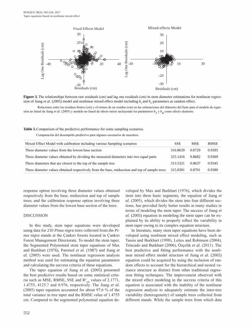
Figure 3. The relationships between raw residuals (cm) and lag one residuals (cm) in stem diameter estimations for nonlinear regres-sion of Jiang et al. (2005) model and nonlinear mixed effect model including b1 and b4 parameters as random effect. Relaciones entre los residuos brutos (cm) y el retraso de un residuo (cm) en las estimaciones del diámetro del fuste para el modelo de regre-sión no lineal de Jiang et al. (2005) y modelo no lineal de efecto mixto incluyendo los parámetros b1 y b4 como efecto aleatorio.

-30

-20

-10

0

10

20

30

-40 -20 0 20 40

Lag

One

Res

idua

ls (c

m)

Residuals (cm)

Fixed Effects Model

-30

-20

-10

0

10

20

30

-30 -10 10 30

Lag

One

Res

idua

ls (c

m)

Residuals (cm)

Mixed-effects Model

Table 5. Comparison of the predictive performance for some sampling scenarios. Comparación del desempeño predictivo para algunos escenarios de muestreo.

Mixed Effect Model with calibration including various Sampling scenarios SSE MSE RMSE

Three diameter values from the lowest base section 316.8639 0.8729 0.9395

Three diameter values obtained by dividing the measured diameters into two equal parts 315.1416 0.8682 0.9369

Three diameters that are closest to the top of the sample tree 313.5321 0.8637 0.9345

Three diameter values obtained respectively from the base, midsection and top of sample trees 315.8381 0.8701 0.9380

response option involving three diameter values obtained respectively from the base, midsection and top of sample trees; and the calibration response option involving three diameter values from the lowest base section of the trees.

DISCUSSION

In this study, stem taper equations were developed using data for 210 Pinus nigra trees collected from the Pi-nus nigra stands at the Çankırı forests located in Çankırı Forest Management Directorate. To model the stem taper, the Segmented Polynomial stem taper equations of Max and Burkhart (1976), Parresol et al. (1987) and Jiang et al. (2005) were used. The nonlinear regression analysis method was used for estimating the equation parameters and calculating the success criteria of these equations.

The taper equation of Jiang et al. (2005) presented the best predictive results based on some statistical crite-ria such as MSE, RMSE, SSE and R2

adj values of 2.1771, 1.4755, 4125.7 and 0.976, respectively. The Jiang et al. (2005) taper equation accounted for about 97.6 % of the total variance in tree taper and the RMSE value of 1.4755 cm. Compared to the segmented polynomial equation de-

veloped by Max and Burkhart (1976), which divides the stem into three basic segments, the equation of Jiang et al. (2005), which divides the stem into four different sec-tions, has provided fairly better results in many studies in terms of modeling the stem taper. The success of Jiang et al. (2005) equation in modeling the stem taper can be ex-plained by its ability to properly reflect the variability in stem taper owing to its complex equation structure.

In literature, many stem taper equations have been de-veloped using nonlinear mixed effect modeling, such as Tassia and Burkhart (1998), Leites and Robinson (2004), Trincado and Burkhart (2006), Özçelik et al. (2011). The best predictive and fitting performance with the nonli-near mixed effect model structure of Jiang et al. (2005) equation could be acquired by using the inclusion of ran-dom effects to account for the hierarchical and nested va-riance structure as distinct from other traditional regres-sion fitting techniques. The improvement observed with the mixed effect modeling in the success criteria of this equation is associated with the inability of the nonlinear regression analysis to adequately estimate the inter-tree variability (heterogeneity) of sample trees collected from different stands. While the sample trees from which data


552

were obtained within the scope of the study were homo-genous within themselves (intra-homogenous), they were heterogeneous between each other (inter-heterogeneous), which indicated a hierarchal data structure. This problem designated as autocorrelation, can either cause a systema-tic error in the estimation of the confidence intervals for the equation parameters, or negatively affect the reliability of the regression model results (Searle et al. 1992). In the stem taper equations developed based on measurements performed on sample trees cut from different stands and cultivation environments, the use of the mixed effect non-linear regression analysis may improve the taper predic-tion in future studies.

When evaluating the calibration responses of the mixed effect models, the most important point to determine is the type of diameters that will be measured on the trees when calibrating the mixed effect model to a certain stand or fo-rest sites. In our study, the first calibration option involved three diameters measured from the lowest base section of the trees; the second calibration option involved three dia-meters that divided the tree into two equal parts; the third calibration option involved three diameters closest to the top of the trees; and the fourth calibration option involved three diameter values measured respectively at the base, midsection and top of the trees. Comparisons performed according to different statistical criteria have shown that the best model estimation results are obtained with the ca-libration option where three diameters are measured at the top of the trees. However, Trincado and Burkhart (2006) have determined the calibration response by using the stem diameter at different heights such as a single diameter at 2.4 m, 3.7 m, 4.9 m or 6.1 m height, and two diameters measured at 3.7 m and 6.1 meter height. Yang et al. (2009) have analyzed the calibration responses by using many di-fferent diameters measured at 0.3, 1.3, 2.8, 5.3, 7.8, 10.3, 12.8, 15.3, 17.8, 20.3 and 22.8 meter. Lejeune et al. (2009) calibrated the stem taper equations by measuring a single diameter at heights of 3, 5, 7 and 10 meters, and two dia-meters at heights between 3.5 meters and 7 meters, and between 3.5 meters and 10 meters. Sharma and Parton (2009) analyzed the calibration responses of mixed effect modeling, based on the single diameter measurement of 9 different choices, the two-diameter measurement of 18 different choices, and the three-diameter measurement of 47 different choices. Özçelik et al. (2011) calibrated stem taper equations using tapers measured at 3.3 m and 6.3 m. In addition, with the calibration of the models, better results were obtained compared to the nonlinear regres-sion analysis and the model estimations in which the mi-xed effect random effect parameter which is not calibrated by using sub-sample trees. In many other studies such as Trincado and Burkhart (2006), Yang et al. (2009), Lejeune et al. (2009), Sharma and Parton (2009), it was similarly determined that calibration for the mixed effect model by using additional diameter measurements resulted in best predictive model estimation.

Stem taper equations specifically, which allow the de-tailed estimation of stem volumes, may enable Turkish fo-restry operations to estimate volume more accurately and consistently. In Turkey, with the growing importance of the sale of planted trees, there is a growing need to have detailed and accurate volume estimations before the tree is even cut; in this regard, the use of stem taper equations be-comes even more important. Developing stem taper equa-tions for the different cultivation environments and stands in which different tree species, especially domestic trees, are grown is a significant priority.

ACKNOWLEDGMENT

We would like to thank the Çankırı Karatekin Uni-versity Project Department (CAKU-BAP), Project No: OF090316B05, for their support.

REFERENCES

Calama R, G Montero. 2004. Interregional nonlinear height– diameter model with random coefficients for stone pine in Spain. Canadian Journal of Forest Research 34:150-163.

Castedo-Dorado F, U Diéguez-Aranda, M Barrio, M Sánchez, K von Gadow. 2006. A generalized height-diameter model in-cluding random components for radiata pine plantations in northeastern Spain. Forest Ecology and Management 229: 202-213.

Clark A, RA Souther, BE Schlaegel. 1991. Stem profile equa-tions for southern tree species. Res. Pap. SE-282. Ashevi-lle, USA. U.S. Department of Agriculture, Forest Service, Southeastern Forest Experiment Station. 117 p.

Crecente-Campo F, M Tomé, P Soares, U Diéguez-Aranda. 2010. A generalized nonlinear mixed-effects height-diameter mo-del for Eucalyptus globulus L. in northwestern Spain. Fo-rest Ecology and Management 259: 943-952.

Czaplewski RL, JP Mcclure. 1988. Conditioning a segmented stem profile model for two diameter measurement. Forest Science 34(2): 512-522.

Davis PH. 1982. Flora of Turkey and East Aegean Islands. Edinburgh , UK. University Press.

Demaerschalk JP, A Kozak. 1977. The whole-bole system, a con-ditional dual-equation system for precise prediction of tree profiles. Canadian Journal of Forest Research 7: 488-497.

General Directorate of Forestry 2015. Criteria and indicators for sustainable forest management report for 2015. Ankara, Turkey. General Directorate of Forest Publications.

Jiang L, JR Brooks, J Wang. 2005. Compatible taper and volume equations for yellow-poplar in West Virginia. Forest Ecolo-gy and Management 213: 399-409.

Lappi J. 1991. Calibration of height and volume equations with random parameters. Forest Science 37(3): 781-801.

Lappi J. 1997. A longitudinal analysis of height–diameter curves. Forest Science 43: 555-570.

Lejeune G, CH Ung, M Fortin, XJ Guo, M C Lambert, JC Ruel, 2009. A simple stem taper model with mixed effects for boreal black spruce. European Journal of Forest Research 128(5): 505-513.

Leites LP, AP Robinson. 2004. Improving taper equations of lo-


553

blolly pine with crown dimensions in a mixed-effects mo-deling framework. Forest Science 50: 204-212.

Littell RC, GA Miliken, WW Stroup, RD Wolfinger. 2005. SAS system for Mixed Models. Cary, USA. SAS Institute Inc.

Max TA, HE Burkhart. 1976. Segmented polynomial regression applied to taper equations. Forest Science 22(3): 283-289.

Özçelik R, JR Brooks, L Jiang. 2011. Modeling stem profile of Lebanon cedar, Brutian pine, and Cilicica fir in Southern Turkey using nonlinear mixed-effects models. European Journal of Forest Research 130: 613-621.

Özçelik R, JR Brooks. 2012. Compatible volume and taper mo-dels for economically important tree species of Turkey. An-nals of Forest Science 69: 105-118.

Parresol BR, JE Hotveld, QV Cao. 1987. A volume and taper prediction system for bald cypress. Canadian Journal of Forest Research 17: 250-259.

Pinheiro JC, DM Bates. 2000. Mixed-Effects Models in S and S-PLUS. Springer.

SAS Institute Inc. 2013. SAS/IML 9.3 User’s Guide. Cary, USA. SAS Institute Inc. 1097 p.

Searle SR, G Casella, CE Mc Culloch. 1992. Variance compo-nents. Hoboken, USA. John Wiley. 501 p.

Şenyurt M, I Ercanlı, F Bolat. 2014. Developing Stem taper and stem volume equations using Nonlinear Mixed Effect Mode-

ling Approach for Crimean Pine Stands [Pinus nigra Arnold. subsp. pallasiana (Lamb.) Holmboe]. Çankırı, Turkey. Central Forest Sub-District Directorate, Çankırı Karatekin University Project Report (CAKU-BAP), Project No: OF090316B05.

Sharma M, J Parton. 2009. Modeling Stand Density Effects on Taper for Jack pine Black spruce plantations Using Dimen-sional Analysis. Forest Science 55(3): 268-282.

Tassia G, HE Burkhart. 1998. An application of mixed effects analysis to modeling thinning effects on stem profile of lo-blolly pine. Forest Ecology and Management 103: 87-101.

Trincado G, HE Burkhart. 2006. A generalized approach for mo-deling and localizing stem profile curve. Forest Science 52: 670-682.

Trincado G, CL VanderSchaaf, HE Burkhart. 2007. Regional mi-xed-effects height-diameter models for loblolly pine (Pinus taeda L.) plantations. European Journal of Forest Research 126: 253-262.

Yang Y, S Huang, G Trincado, SX Meng. 2009. Nonlinear Mixed Effects Modelling of Variable Exponent Taper Equations for Lodgepole pine in Alberta, Canada. European Journal of Forest Research 128: 415-429.

Yavuz H. 1995. Compatible and noncompatible taper models. Trabzon, Turkey. Faculty of Forestry, Karadeniz Technical University. p. 101-106.

Recibido: 13.07.17Aceptado: 11.09.17


554

Documents

Taper equations based on nonlinear mixed effect … · de datos de validación, el esquema de muestreo con tres submuestra de diámetro superior en un árbol produjo los mejores resultados