Table 1Payoff Matrix

A’s Profit (Top) B’s Profit (Bottom)

² Pa ÷

$11.20 $11.40 $11.60 $11.80 $12.00 $12.20 $12.40 $12.60 $12.80 $13.00 $13.20

$17.00 $11.49 $12.56 $13.32 $13.77 w $13.91 $13.73 $13.24 $12.44 $11.33 $9.91 $8.17

-$16.94 -$14.70 -$12.52 -$10.37 -$8.28 -$6.23 -$4.22 -$2.25 -$0.32 $1.56 $3.41

$16.80 $10.66 $11.69 $12.40 $12.80 w $12.89 $12.67 $12.13 $11.28 $10.12 $8.65 $6.87

-$14.58 -$12.40 -$10.26 -$8.17 -$6.12 -$4.12 -$2.16 -$0.24 $1.64 $3.48 $5.28

$16.60 $9.82 $10.79 $11.46 $11.81 w $11.85 $11.58 $11.00 $10.10 $8.90 $7.38 $5.55

-$12.42 -$10.29 -$8.20 -$6.16 -$4.17 -$2.21 -$0.30 $1.57 $3.40 $5.20 $6.96

$16.40 $8.96 $9.89 $10.50 w $10.81 $10.80 $10.48 $9.85 $8.91 $7.65 $6.09 $4.21

-$10.46 -$8.38 -$6.35 -$4.36 -$2.41 -$0.51 $1.36 $3.18 $4.97 $6.72 $8.43

$16.20 $8.08 $8.96 $9.53 w $9.79 $9.73 $9.36 $8.68 $7.69 $6.39 $4.77 $2.84

-$8.70 -$6.68 -$4.69 -$2.76 -$0.86 $1.00 $2.81 $4.59 $6.33 $8.03 $9.70

$16.00 $7.19 $8.02 $8.54 w $8.75 $8.64 $8.22 $7.49 $6.45 $5.10 $3.43 $1.45

-$7.14 -$5.17 -$3.24 -$1.35 $0.50 $2.30 $4.07 $5.80 $7.49 $9.15 $10.77

$15.80 $6.29 $7.07 $7.53 w $7.69 $7.53 $7.07 $6.29 $5.19 $3.79 $2.07 $0.04

-$5.78 -$3.86 -$1.98 -$0.15 $1.65 $3.41 $5.13 $6.81 $8.46 $10.07 $11.65

$15.60 $5.36 $6.09 $6.51 w $6.61 $6.41 $5.89 $5.06 $3.91 $2.46 $0.69 -$1.39

-$4.62 -$2.75 -$0.93 $0.86 $2.61 $4.31 $5.98 $7.62 $9.22 $10.78 $12.32

$15.40 $4.42 $5.10 $5.46 w $5.52 $5.26 $4.69 $3.80 $2.61 $1.10 -$0.72 -$2.85

-$3.66 -$1.85 -$0.07 $1.66 $3.36 $5.02 $6.64 $8.23 $9.78 $11.30 $12.79

$15.20 $3.46 $4.09 $4.39 w $4.40 $4.09 $3.47 $2.53 $1.28 -$0.28 -$2.15 -$4.33

-$2.90 -$1.14 $0.59 $2.27 $3.91 $5.52 $7.10 $8.64 $10.14 $11.62 $13.06

$15.00 $2.48 $3.06 w $3.32 $3.26 $2.90 $2.22 $1.24 -$0.06 -$1.68 -$3.60 -$5.84

-$2.34 -$0.63 $1.04 $2.67 $4.27 $5.83 $7.36 $8.85 $10.31 $11.74 $13.13

$14.80 $1.49 $2.01 w $2.21 $2.11 $1.69 $0.96 -$0.08 -$1.44 -$3.10 -$5.08 -$7.37

-$1.98 -$0.32 $1.30 $2.88 $4.42 $5.93 $7.41 $8.86 $10.27 $11.65 $13.01

$14.60 $0.47 $0.94 w $1.09 $0.93 $0.46 -$0.33 -$1.42 -$2.83 -$4.55 -$6.58 -$8.93

-$1.82 -$0.22 $1.35 $2.88 $4.38 $5.84 $7.27 $8.67 $10.03 $11.37 $12.68

$14.40 -$0.56 -$0.15 w -$0.06 -$0.27 -$0.80 -$1.64 -$2.79 -$4.25 -$6.03 -$8.12 -$10.52

-$1.86 -$0.31 $1.21 $2.69 $4.13 $5.55 $6.93 $8.28 $9.60 $10.89 $12.15

$14.20 -$1.62 -$1.27 w -$1.22 -$1.50 -$2.08 -$2.97 -$4.18 -$5.70 -$7.53 -$9.67 -$12.13

-$2.10 -$0.60 $0.86 $2.29 $3.69 $5.05 $6.38 $7.69 $8.96 $10.21 $11.42

$14.00 -$2.69 w -$2.40 -$2.41 -$2.74 -$3.38 -$4.33 -$5.60 -$7.17 -$9.06 -$11.26 -$13.77

-$2.54 -$1.09 $0.32 $1.70 $3.04 $4.36 $5.64 $6.90 $8.12 $9.32 $10.50

Abstract: This paper shows how principles and intermediate students can gain a feel for strategic

price setting by playing a relatively large oligopoly game. A playoff matrix is constructed, and

various strategies and outcomes are discussed. The game is extended to a continuous price

space, and various applications appropriate for intermediate micro students are outlined. Finally,

in order to make it easier for others to tinker with the assumptions of the game, I can provide the

Mathematica code used to generate the table and figures.

Keywords: oligopoly; duopoly; game theory; strategic behavior.

JEL Codes:

An Extended Duopoly Game

by

John C. EckalbarProfessor of Economics

California State UniversityChico, CA 95929

530-343-6791jeckalbar@aol.com

January 17, 2001

1

An Extended Duopoly Game

Firms in an oligopoly cannot maximize their profits by following simple rules, such as

marginal revenue equals marginal cost. Instead, they are forced to think strategically. When they

contemplate an action, such as a price change, they must consider the reaction of their rivals,

because the effect of the price change will depend critically upon the behavior of the rival after

the change. Making this fact come alive in a principles or intermediate micro class can be a

challenge.

Most texts present one or two oligopoly games to give the student a feel for the issues.

These games generally consist of two-by-two payoff matrices, and my experience with them is

that they are too small and simple to get the students involved.1 In this article I report on the use

of a much larger and richer payoff matrix for the study of strategic duopoly price-setting

behavior. I have found it useful in both principles and intermediate micro classes, and I expect

that it would also be valuable in making tangible some of the more abstract issues in a game

theory class.2

After I present and discuss the uses of a relatively large payoff matrix suitable for a

principles class, I consider some features of the underlying game in a continuous price space.

The generalization can be studied in an intermediate micro class.

USING A LARGE PAYOFF MATRIX

The exercise is started by giving the students an unmarked version of Table 1.3 I explain

that we are considering a duopoly, that is, an oligopoly with two firms in the industry. The two

firms produce similar products, which the buyers regard as substitutes. The table shows firm A’s

price in bold along the top and B’s price in bold along the left-hand edge. Each firm’s sales

depend upon the price it charges as well as the price its rival charges. When both prices are set,

demand quantities, revenues, costs, and profits are determined. The values for Pa and Pb

2

determine our “address,” or fix our position in the table. Each position in the table shows a pair

of numbers. The number on the top is A’s profit or loss, and the number on the bottom is B’s,

when A charges the price shown at the top and B charges the price written at the left. For

example, when Pa is $12.40 and Pb is $15.60, A’s profit is $5.06 and B’s is $5.98.

The students are curious about where these numbers have come from, and I tell them that

I made them up, or more accurately, I made up some demand and cost equations that seemed

reasonable, and then I used Mathematica to crunch out the numbers.4 Because the students are

generally impatient to get on with the game, I simply draw their attention to a few general

features of the table. For instance, suppose Pb is fixed at, say, $16. This locks us onto a row in

the table, and by changing Pa, firm A has the ability to slide us left and right. Starting from a low

price of $11.20, as firm A increases Pa, A’s profit rises to a peak of $8.75 at Pa = $11.80 and

then falls off as Pa continues to rise (i.e., as we move further to the right). This is exactly what

you would expect from looking at the standard graphical presentations of demand, cost, and

profits. When Pb is fixed, A’s demand curve is locked in place. Then A has a single best price

at the output level where MR = MC, and as the price varies from the optimum, profits drop off.

You can see the same pattern for B’s profit by looking up and down any column. The other

feature to notice is that A’s profit improves as we move up the columns, and B’s profit rises as

we move to the right. For example, when B raises price, some of B’s customers choose to buy

from A, and this raises A’s demand and A’s profit.

Given just these preliminaries, I divide the class into two groups, the A’s and the B’s. I

generally have a class of about thirty students, with about fifteen per team. In larger classes, I

might run several games concurrently, with opposing teams of ten to fifteen students each. As

long as the team is about fifteen or fewer students, there seems to be an easy flow of dialogue

between the team members. Students in larger groups are often less willing to communicate.

3

Having several pairs of smaller opposing teams has its pro’s and con’s–smaller teams mean more

individual participation, but more simultaneous games tends to create bedlam in the classroom.

I start them off at an arbitrary initial cell. For instance, I might say that Pa = $12.80 and

Pb = $16.60. In the beginning we will be civil and take turns adjusting price, as if we were two

gas stations across the street from one another posting prices and then waiting to see what our

rival does. Let the A’s go first. Invariably the A’s talk it up amongst themselves and agree to cut

the price to $12.00 in order to raise their profits from $8.90 to $11.85. When the B’s get their

turn they typically cut price from $16.60 to $14.80 in order to convert their $4.17 loss to a profit

of $4.42. The A team then cuts price to $11.60, and the B’s follow with a cut to $14.60. Once

we get to the $11.60/$14.60 cell, things come to a stop. Someone invariably suggests that we

have found “the equilibrium,” but I caution that we will find many different sorts of equilibria

depending upon the strategies they employ. At the moment I will only say that we have found

the “follower/follower” or Nash equilibrium–A is at an optimum, given B’s current choice, and B

is likewise at an optimum, given the behavior of A. Students are warned not to think of this

point as the equilibrium.

I’ll give them another starting point, and let the game continue. Perhaps we start at Pa =

$11.20 and Pb = $15.40. B goes first, and before long we are back at the $11.60/$14.60 cell.

After a few more tries, their attention is fixed on $11.60/$14.60. At this point, they seem

genuinely curious about what’s going on there?

The next step is to define each firm’s “reaction function.” Firm A has a maximum-profit

cell in each row, that is, for any given Pb, there will be a Pa that maximizes A’s profit. The set

of all these cells is A’s reaction function. These cells are marked with an asterisk (*) in Table 1.

If B were to fix price, A would like to slide left or right to get onto A’s reaction function.

Similarly, B has a maximum-profit cell in each column, and the collection of these cells (shown

4

by a heavy box in Table 1) is B’s reaction function. The $11.60/$14.60 cell is at the intersection

of the reaction functions, and the orientation of the reaction functions, together with the students’

behavior have led us to the $11.60/$14.60 cell. More on this shortly.

The students are not yet thinking strategically. They are behaving as “followers.” For

instance, suppose we sit at Pa = $12.60 and Pb = $16.20, and it is A’s move. Early in the game,

firm A is likely to cut price to $11.80, thinking it will be increasing its profits from $7.69 to

$9.79. The problem is that firm A is not anticipating the reaction of its rival. If firm A were

thinking strategically, it would compare its initial profits with the profits it would earn following

B’s most likely reaction. For instance, if B cut price to $14.60 following A’s cut to $11.80, A’s

profit would be only $0.93, which is far worse than its original profits. Once this point is made

in the classroom, the students generally behave quite differently, and there is much more

discussion within each team prior to a price move.

The discussion up to this point takes about forty-five minutes. I generally set my class

schedule so that the class ends at this point, and the students are instructed to return to the next

class with three written strategy suggestions for their teams.

At the start of the next class I review the rules and collect the homework. I then re-form

the teams and let the game begin. I will let the firms adjust prices at will, no longer requiring

that they take turns. It often happens that one of the firms will discover that there might be an

advantage to behaving malevolently. Suppose, for instance, we are at the follower/follower

solution. Someone on the B team might notice that if the B’s cut price to $14.40, the A’s will

lose money, even if they stay on their reaction function, while the B’s will make money. The A’s

quickly realize that if they stay at Pa = $11.60 with Pb = $14.40, the A’s will go broke, whereas

the B’s continue to make a profit. This generally prompts the A’s to cut price to $11.40, even

though that makes their loss worse, because it now causes B to lose money. In fact if B stayed

5

there, B would now lose more than A. This may prompt a further cut by B. We are now in the

midst of a price war, with each team heading toward the bottom left margins of the table.

The table alone does not have enough information to determine who will win the price

war, but at least it prompts a discussion of the subject. With just a little prodding, the students

will bring up other factors, such as liquid assets, lines of credit, and the advantage of having low

cost at the start of any price war. The case of People’s Express and United Airlines might be

mentioned. We could also talk about an arms race.

When the students have tired of trying to ruin each other, I will pick them up and drop

them in the top right portion of the figure once again, for instance, at Pa = $12.80 and Pb =

$16.20. This time they are much more circumspect about their moves, and there is a lot of

discussion along the lines of, “If we do that, what are they going to do?” They are now learning

the meaning of strategy. They have seen the game degenerate to a point where neither player is

doing well, and they are reluctant to “rock the boat” when things are going relatively well. At

this stage in the course, we have already covered the theory of the kinked demand curve, and we

are now prepared to see oligopoly price stickiness in a new light. Perhaps a fear of precipitating

a price war would justify a policy of leaving well enough alone when conditions are tolerable.

But generally, a little time draws us slowly back toward the follower/follower solution, or worse.

When things again degenerate, I will read them the now-famous transcript of the

conversation between Robert Crandall, the President of American Airlines, and Howard Putnam,

the President of rival Braniff. I warn the students (with a wink) that there is some high level

business-speak in the conversation between these two CEOs, and that they, as mere students,

might not catch on to everything.

Mr. Crandall says, “I think it’s dumb as hell . . . to sit here and pound the s--- out of each

other and neither one of us making a (deleted) dime. . . . We can both live here and there ain’t no

6

room for Delta. But there’s, ah, no reason that I can see, all right, to put both companies out of

business.”

Mr. Putnam replies, “Do you have a suggestion for me?”

Crandall’s response is: “Yes. I have a suggestion for you. Raise your goddamn fares

20%. I’ll raise mine the next morning. . . . You’ll make more money and I will too.”

Mr. Putnam says, “We can’t talk about pricing.”

Mr. Crandall replies, “Oh, Bulls---, Howard. We can talk about any g--damn thing we

want to talk about.” (Quoted in The Wall Street Journal, February 24, 1983, p. 2.)

To the legally naive, this may sound like an attempt to fix prices, but this is not what the

courts found.5 American Airlines is now the second largest airline in the world, and Braniff is

bankrupt.

Now I will have the A’s take the role of American Airlines and the B’s play the part of

Braniff. I ask them to imagine that Mr. Putnam agreed to meet Mr. Crandall and discuss a price

setting deal. I ask each team to make a concrete proposal to the other side, something like, “We

will charge _____, if you will charge _____.”

The students seem to enjoy this simulated clandestine activity. They begin looking in the

upper right corner of the matrix, and inevitably each side looks for a cell that offers better profits

for both of them, but gives a slight advantage to the team making the proposal. For instance, the

A’s might propose Pa = $12.80 and Pb = $16.40, while the B’s favor something more like Pa =

$12.80 and Pb = $16.00. They typically wrangle back and forth, sometimes threatening the other

side with a price war if the last offer is refused. The cell at Pa = $12.80 and Pb = $16.20 usually

gets a lot of attention, because profits are about evenly split at that location.

This is a good point to discuss cartels and joint profit maximum. The two firms might

adopt a strategy of searching for the cell that brings in the largest total profit, that is, the cell that

7

maximizes the sum of A’s profit and B’s profit. Once they have gotten the maximum from their

customers, they might then decide to redistribute the sub-totals, but at least then they would be

arguing about cutting up the biggest possible pie. The joint profit maximizing cell is at Pa =

$13.00 and Pb = $16.40, where A earns $6.09 and B gets $6.72. The B’s seem happy, but the

A’s argue about how big a kickback they deserve for going to this cell. In fact, the jealousy of

the A’s seriously undermines the establishment of the joint profit outcome. Note that this issue

would not arise in a symmetric payoff matrix.

There are several lessons to be drawn at this stage. First, it is difficult for the two firms to

reach an agreement. Each firm wants to bias the deal in its own favor, and neither is eager to

concede the advantage to the other. Second, these deals are illegal, so they cannot be enforced in

the courts, and there is a real risk of being caught and prosecuted. Third, and most important,

once a deal is struck, it is unstable; that is, it tends to unravel of its own accord as the dissimilar

interests of the two firms pull them in other directions.

Suppose, for example, the firms settle at the point Pa = $12.80 and Pb = $16.20. Each is

doing quite well in comparison with the follower/follower solution or in comparison with a price

war, but each is also tempted to cheat on the deal, and there is no enforceable contract to prevent

it. Firm A sees its profit rising as it slides to the left, cutting price, whereas B is tempted to move

downward. If both of them give in to the temptation, we move back down and left, with profits

for each firm falling. This is a good spot to bring up the history of OPEC, to talk about how the

cartel has followed a pattern of formulating an agreement and holding prices and profits up for a

while, only to be followed by an erosion of their position, then perhaps another deal, followed by

another erosion, and so on. It’s the myth of Sisyphus. They can roll the ball to the top of the hill

(upper right corner of the matrix), but inevitably it rolls back down.

I ask the students what other options are available, and someone always suggests that one

8

of the companies might buy the other. This prompts some interesting discussions. Suppose, for

instance, we are at the follower/follower solution with A making $1.09 and B making $1.35.

Suppose B wants to buy A and operate it as a separate, autonomous division. What is a fair price

for firm A? A finance major might suggest that firms are “worth” about 25 times earnings these

days, so the stock of firm A might be worth 25 x $1.09 = $27.25. Someone on the A team will

reply, “Yes, but once you buy us and we no longer compete, you can set both prices, and earnings

from the A division will be over $6, plus B division earnings will be much better without

competition from A. So maybe a stock price of at least 25 x $6 = $150 is in order. That certainly

leaves a lot of room for negotiation. And it also provides an opportunity to discuss antitrust

policy in light of recent mergers and proposed mergers.

One strategy that students are unlikely to devise on their own is Stackelberg-type price

leadership. I will suggest the following: What if B decided to fix price at some level and then

simply refused to adjust it any further. And at the same time, firm A decided to quit fighting and

simply charge the best price it could, given B’s price. Here B is the leader, and A is the follower.

What price would B set? With just a little reflection, the students realize that B must search A’s

reaction function for the cell that yields the largest profit for B. This occurs when Pb = $15.20.

So if B sets its price at $15.20, A will charge $11.80. Profits now are $4.40 for A and $2.27 for

B. If A leads and B follows, the players go to Pa = $12.00 and Pb = $14.80.

Why would price leadership emerge as a strategy? What are its advantages? First, it

would be harder to prosecute, because the firms do not have to make contact with each other and

negotiate the prices. There will be no smoking gun, or taped phone call. Second, both firms do

better under price leadership than they do under the follower/follower option. In this particular

game, the follower makes out relatively better than the leader, and that may make both firms

reluctant to lead, but other numerical assumptions could lead to other results.

The second day of game playing takes about thirty minutes. In a principles class, I will

9

put the payoff matrix aside at this point and delve into a graphical analysis of models of price

leadership by a dominant firm and cartel profit maximization, using familiar demand and cost

curves. My impression is that these topics go over much better once the students have had some

first-hand experience with these situations. In a more advanced class, I will translate the game

into a continuous (Pa, Pb) space.

DUOPOLY GAME IN CONTINUOUS PRICE SPACE

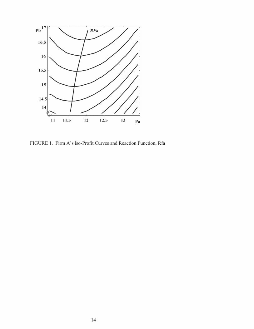
The first step in the continuous-case discussion is to derive the iso-profit curves, and then

find the reaction functions from them. A mathematical derivation of the iso-profit curves is

generally beyond the level of an intermediate class, but the table suggests that, for instance, A’s

curves take on the appearance shown in Figure 1. Profits rise as we move up in the figure. A’s

reaction function is the locus of zero-slope points on A’s iso-profit curves, that is, the locus of

points at which A’s profits are at a maximum given a fixed price from B. B’s iso-profit curves

and reaction function, not shown here, are similar to A’s, but rotated ninety degrees clockwise.

If we combine the two reaction functions, we can see what generally happens in the early

stages of the game. The two reaction functions together with some sample paths toward the

follower/follower equilibrium are shown in Figure 2. The shaded areas in the acute regions

between the reaction functions constitute a strongly attractive set. Given the way the students

generally begin playing the game, if we are not in the set, we are attracted to it, and once we are

drawn into it, we remain within it and converge to the intersection of the reaction functions.

When we begin at point 1, the A team is attracted to point 2. Since they like point 2 better than

point 1, they cut their price. But when B responds, we go to point 3. If the A-team were thinking

strategically, it would compare point 3 with point 1, rather than point 2 with point 1.

Suppose B is the price leader. We then want to know where B’s profits reach a maximum

along A’s reaction function. We can visualize this by superimposing B’s iso-profit curves over

A’s reaction function. If B leads, then B is looking for the point of tangency between its iso-

10

profit curves and A’s reaction function, as shown in Figure 3.

If we combine the two sets of iso-profit curves, we get Figure 4. When students first see

Figure 4, someone is likely to say that is looks like an Edgeworth box. That is an insight that is

worth building upon. Suppose, for instance, that the two firms are presently at point X in the

figure. With appropriate price increases, they could move into the shaded region where both

firms will earn higher profits. This is reminiscent of a “better set” in an Edgeworth box. The

dashed line running through points T, Y, and V is analogous to a contract curve; that is, iso-profit

curves are tangent to each other at points on this line, so it is not possible for firms to adjust

prices so that both firms end up making higher profits. The cartel joint-profit maximum will be

on this line. The equations used to generate our data give a cartel maximum profit at point Y,

with Pa = $12.97 and Pb = $16.2873. Notice that both firms are tempted to cheat on the cartel

prices. Firm A is enticed leftward toward higher iso-profit curves, and B is attracted downward.

EXTENSIONS

I believe that a large oligopoly game makes it possible for students to experience a rich

array of oligopoly strategies and outcomes. And this is a good thing. With a little coaching on

the use of Mathematica, it is relatively easy for the instructor to tinker with, tune, and visualize a

wide variety of situations.

In a class with more than a day or two to cover the topic, other exercises might be tried. For

instance, the payoff matrix might be subdivided so that each team only sees its own profits. How

does this reduction in information effect the outcome? Or carrying that a step further, the professor

might not reveal any of the payoff matrix in advance, but rather provide profit information to the

players only after they have made their choices, leaving it to them to grope toward an acceptable

outcome. Though it would be hard to present the game graphically, more advanced classes could

play the game with three or more firms by generalizing the demand equations and generating profit

outcomes numerically with computers or programmable calculators.

11

REFERENCES

Boyd, D. W. 1998 On the use of symbolic computation in undergraduate microeconomics

instruction. Journal of Economic Education 29 Summer : 227-46.

Dixit, A. and S. Skeath. 1999. Games of strategy. New York: W. W. Norton.

Dolbear, F. T., L. B. Lave, G. Bowman, A. Lieberman, E. Prescott, F. Rueter, and R. Sherman.

1968. Collusion in oligopoly: An experiment on the effect of numbers and information. Quarterly

Journal of Economics 82 (May): 240-59.

Dutta, Prajit K. 1999. Strategies and games. Cambridge: MIT Press.

Kagel, J. H. and A. E. Roth, eds. 1997. Handbook of experimental economics. Princeton: Princeton

University Press.

Varian, H., ed. 1992. Economic and financial modeling with Mathematica. New York: Springer-

Verlag.

Varian, H. 1996. Intermediate microeconomics. New York: W. W. Norton.

12

NOTES

1. Of course there are exceptions, particularly in the experimental economics literature. Dolbear, et

al. (1968) report on an experimental pricing exercise involving a large payoff matrix, though their

focus is more on the number of firms in the industry and the extent of available information. See

also Kagel and Roth (1997).

2. Game theory texts such as Dixit and Skeath (1999) and Dutta (1999) generally don’t contain any

large payoff matrices, so they lose the chance to let the intuitive appeal of the discrete game

illuminate the more abstract content of the continuous function. With a large game it is relatively

easy to see how a function, such as a reaction function, resides in the payoff matrix. This is likely to

be helpful for students new to game theory.

3. An unmarked version of the table is available at

http://www.csuchico.edu/econ/Faculty/Matrix.htm.

4. The functions used to generate the table and figures are as follows: A’s demand, Qa, is given by

30 !3Pa + 50Pb/(Pb+15). Notice that as Pb approaches infinity, the final term in the equation

approaches 50, that is, as B raises price and chases away his own customers, there is a limit to how

much effect is felt by A. Also, as Pb heads toward zero, A’s demand falls toward 30 ! 3Pa. A’s

total cost is given by 170 + Qa + Qa2/10, and profit has the obvious definition. The parallel

functions for B are: Qb = 26 + 40Pa/(Pa+10) ! 2Pb for demand and 205.5 + Qb + Qb2/8, for cost.

The figures and table were generated using Mathematica, though a simple spreadsheet would work

just as well for the table. The Mathematica code used is available on request from the author.

5. This is not the place, and I am not the person, to wade into the legal details of the case, but the

brief history goes like this: The telephone conversation between Crandall and Putnam took place

February 1, 1982. After Putnam turned over the tape, the U. S. Government brought suit against

American Airlines. (570 F. Supp. 654; 1983 U.S. Dist.) The suit was dismissed September 12,

13

1983, on the grounds that, although Mr. Crandall might have “solicited” Mr. Putnam to raise prices,

this did not constitute an “attempt” to raise prices under Section 2 of the Sherman Act. The U. S.

appealed, and on October 15, 1984, the United States Court of Appeals for the Fifth Circuit vacated

the lower court’s dismissal. (743 f.2d 1114; 1984 U.S. app.) American appealed this decision to the

U. S. Supreme Court, which dismissed the Government’s case against American Airlines without

comment on November 22, 1985. (474 U.S. 1001; 106 S. Ct. 420; 1985) The text of these

decisions is available on the Web via Lexis.

14

FIGURE 1. Firm A’s Iso-Profit Curves and Reaction Function, Rfa

15

FIGURE 2. Movement Toward the Reaction Functions andConvergence to the Follower/Follower Equilibrium

16

FIGURE 2. Movement Toward the Reaction Functions andConvergence to the Follower/Follower Equilibrium

17

FIGURE 3. Finding the Price Leadership Solution for B fromA’s Reaction Function and B’s Iso-Profit Curves

18

FIGURE 4. Combining Both Iso-Profit Curves

FIGURE 4. Combining Both Iso-Profit Curves