Department of Civil and Environmental Engineering CHALMERS UNIVERSITY OF TECHNOLOGY Gothenburg, Sweden 2014 REPORT NO. 2014:155

The Influence of Natural and Forced Convection in Attics - A CFD Analysis Master’s Thesis in Applied Mechanics

ANDREAS BENGTSON VICTOR FRANSSON

REPORT NO. 2014:155

The Influence of Natural and Forced Convection in Attics –

A CFD Analysis

ANDREAS BENGTSON

VICTOR FRANSSON

Department of Civil and Environmental Engineering

CHALMERS UNIVERSITY OF TECHNOLOGY

Gothenburg, Sweden 2014

The Influence of Natural and Forced Convection in Attics – A CFD Analysis

ANDREAS BENGTSON

VICTOR FRANSSON

©ANDREAS BENGTSON, VICTOR FRANSSON, 2014.

Technical report no 2014:155

Department of Civil and Environmental Engineering

Chalmers University of Technology

SE-412 96 Göteborg

Sweden

Telephone + 46 (0)31-772 1000

Cover:

Temperature contours for the attic model taken in a vertical plane parallel to the joists

longitudinal direction in the middle of the attic.

This particular case was for the permeability of 4 · 10−8m2,

a temperature difference of 50K and without any ventilation.

Chalmers Reproservice

Göteborg, Sweden 2014

i

The Influence of Natural and Forced Convection in Attics – A CFD Analysis

ANDREAS BENGTSON

VICTOR FRANSSON

Department of Civil and Environmental Engineering

Chalmers University of Technology

Abstract

In this thesis project, the air and heat flow in a principal insulated cold attic model has been numerically

investigated through the use of the commercial CFD software ANSYS Fluent.

A numerical model for the heat transfer has been developed and verified with experiments on a simple

box model containing insulation and an overlying horizontal air cavity.

This numerical model was then applied on a cold attic model with insulation and wooden joists. Both

situations with pure natural convection, caused by the temperature difference between the hot floor of the

attic and the cold roof, as well as situations where the attic in addition was exposed to forced convection in

the form of attic ventilation has been investigated.

This project has been a collaboration between ÅF Industry AB and the Division of Building Technology

at Chalmers University of Technology.

Keywords: Computational Fluid Dynamics, CFD, Building Physics, Heat transfer, Porous Media, Natural

Convection, Forced Convection, Cold Attics

Sammanfattning

I detta examensarbete har luft- och värmeflöden i en förenklad modell av en kallvind undersökts numeriskt

med hjälp av CFD programvaran ANSYS Fluent. En numerisk modell för värmeöverföringen har utvecklats

och verifierats mot experiment på en simpel boxmodell innehållande isolering med ett överliggande

horisontellt luftlager.

Denna beräkningsmodell applicerades sedan på en modell av en kallvind med isolering och träbalkar.

Både situationer med endast naturlig konvektion, orsakad av temperaturskillnaden mellan det varma

golvet och det kalla taket, såväl som situationer då vinden dessutom varit påverkad av påtvingad konvektion

i form av ventilation har undersökts.

Detta projekt har varit ett samarbete mellan ÅF Industry AB och avdelningen för byggnadsteknologi

på Chalmers tekniska högskola.

ii

Thesis Layout

This thesis work is based on the following research papers that have been submitted for publication in

conferences and journals.

• Influence of Heat Transfer Processes in Porous Media with Air Cavity - A CFD Analysis, V. Shankar,

A. Bengtson, V. Fransson&C-EHagentoft, submitted to the conference "8th International Conference

on Computational and Experimental Methods in Multiphase and Complex Flow", 20 - 22 April,

2015, Valencia, Spain

• Numerical Analysis of the Influence of Natural Convection in Attics - A CFD Analysis, V. Shankar,

A. Bengtson, V. Fransson & C-E Hagentoft, submitted to the conference "2015 ASHRAE Annual

Conference", 27 June - 01 July, 2015, Atlanta, GA, USA

• CFD Analysis of Heat Transfer in Ventilated Attics, V. Shankar, A. Bengtson, V. Fransson & C-E

Hagentoft, submitted to the conference "2015 ASHRAE Annual Conference", 27 June - 01 July,

2015, Atlanta, GA, USA

iii

Acknowledgements

We would like to show our gratitude to all those who helped us through this master thesis during the spring

and summer of 2014. Especially, we would like to thank our supervisor at ÅF Industry, Senior Consultant

Vijay Shankar, that initiated this project and made it possible through his guidance and assistance. We

would also like to thank ÅF Industry for the provided computational resources. Furthermore we would

like to thank ÅForsk, Ångpanneföreningens Forskningsstiftelse, for the scholarships that brought us to

Atlanta and the 2014 ASHRAE/IBPSA Building Simulation Conference. We would like to extend our

gratitude to Professor Carl-Eric Hagentoft and the Division of Building Technology at Chalmers University

of Technology for the opportunity to do the master thesis as a collaboration with Chalmers University

of Technology. We would also like to thank Paula Wahlgren for her insightful feedback and comments.

Finally, the computational time on the Glenn cluster provided by C3SE (Chalmers Centre for Computational

Science and Engineering) is greatly acknowledged.

Andreas Bengtson & Victor Fransson, Göteborg 20/9/2014

iv

v

Abbreviations

CFD Computational Fluid Dynamics

Re Reynolds number

AR Aspect Ratio

Ram Modified Rayleigh number

Nu Nusselt number

Nomenclature

µ Dynamic viscosity

ν Kinematic viscosity

Uj Velocity

ρ Density

k Thermal conductivity

cp Specific heat

P Pressure

T Temperature

ε Emissivity

K Permeability

g Gravitational acceleration

β Coefficient of thermal expansion

ϕ Porosity

τij Viscous stress tensor

q Heat flow

dm Material thickness

vi

CONTENTS

Contents

1 Introduction 1

1.1 Previous Research . . . . . . . . . . . . . . . . . . . . . . . . . . . . . . . . . . . . . . 2

1.2 Purpose . . . . . . . . . . . . . . . . . . . . . . . . . . . . . . . . . . . . . . . . . . . 3

1.3 Limitations . . . . . . . . . . . . . . . . . . . . . . . . . . . . . . . . . . . . . . . . . 4

2 Theory 5

2.1 Governing equations . . . . . . . . . . . . . . . . . . . . . . . . . . . . . . . . . . . . 5

2.1.1 Continuity equation . . . . . . . . . . . . . . . . . . . . . . . . . . . . . . . . . 5

2.1.2 Momentum equation . . . . . . . . . . . . . . . . . . . . . . . . . . . . . . . . 5

2.1.3 Energy equation . . . . . . . . . . . . . . . . . . . . . . . . . . . . . . . . . . 5

2.2 Dimensionless numbers . . . . . . . . . . . . . . . . . . . . . . . . . . . . . . . . . . . 5

2.2.1 Modified Rayleigh number . . . . . . . . . . . . . . . . . . . . . . . . . . . . . 6

2.2.2 Nusselt number . . . . . . . . . . . . . . . . . . . . . . . . . . . . . . . . . . . 6

2.2.3 Reynolds number . . . . . . . . . . . . . . . . . . . . . . . . . . . . . . . . . . 6

2.3 Turbulence modeling . . . . . . . . . . . . . . . . . . . . . . . . . . . . . . . . . . . . 6

2.3.1 Standard k − ε model . . . . . . . . . . . . . . . . . . . . . . . . . . . . . . . 6

2.3.2 Modified k − ε model . . . . . . . . . . . . . . . . . . . . . . . . . . . . . . . 7

2.4 The Boussinesq model . . . . . . . . . . . . . . . . . . . . . . . . . . . . . . . . . . . 7

2.5 Mechanisms of heat transfer . . . . . . . . . . . . . . . . . . . . . . . . . . . . . . . . 7

2.5.1 Conduction . . . . . . . . . . . . . . . . . . . . . . . . . . . . . . . . . . . . . 8

2.5.2 Convection . . . . . . . . . . . . . . . . . . . . . . . . . . . . . . . . . . . . . 8

2.5.3 Radiation . . . . . . . . . . . . . . . . . . . . . . . . . . . . . . . . . . . . . . 8

2.6 Boundary Conditions . . . . . . . . . . . . . . . . . . . . . . . . . . . . . . . . . . . . 8

2.7 Modeling of fluid flow in porous media . . . . . . . . . . . . . . . . . . . . . . . . . . 9

2.7.1 Porosity . . . . . . . . . . . . . . . . . . . . . . . . . . . . . . . . . . . . . . . 9

2.7.2 Darcy's law and Permeability . . . . . . . . . . . . . . . . . . . . . . . . . . . 9

2.7.3 Porous media in Fluent . . . . . . . . . . . . . . . . . . . . . . . . . . . . . . . 9

2.8 Radiative heat transfer in Fluent . . . . . . . . . . . . . . . . . . . . . . . . . . . . . . 9

3 Method 11

3.1 Software . . . . . . . . . . . . . . . . . . . . . . . . . . . . . . . . . . . . . . . . . . . 11

3.2 Geometry . . . . . . . . . . . . . . . . . . . . . . . . . . . . . . . . . . . . . . . . . . 11

3.2.1 Insulation Box . . . . . . . . . . . . . . . . . . . . . . . . . . . . . . . . . . . 11

3.2.2 Attic Model . . . . . . . . . . . . . . . . . . . . . . . . . . . . . . . . . . . . . 12

3.3 Mesh . . . . . . . . . . . . . . . . . . . . . . . . . . . . . . . . . . . . . . . . . . . . 14

3.4 Fluent Settings . . . . . . . . . . . . . . . . . . . . . . . . . . . . . . . . . . . . . . . 17

3.4.1 Modeling the Insulation . . . . . . . . . . . . . . . . . . . . . . . . . . . . . . 17

3.4.2 Boundary Conditions . . . . . . . . . . . . . . . . . . . . . . . . . . . . . . . . 18

3.5 Running the Simulations . . . . . . . . . . . . . . . . . . . . . . . . . . . . . . . . . . 19

4 Results 20

4.1 Paper 1 . . . . . . . . . . . . . . . . . . . . . . . . . . . . . . . . . . . . . . . . . . . 20

4.2 Paper 2 . . . . . . . . . . . . . . . . . . . . . . . . . . . . . . . . . . . . . . . . . . . 23

4.3 Paper 3 . . . . . . . . . . . . . . . . . . . . . . . . . . . . . . . . . . . . . . . . . . . 28

vii

CONTENTS

5 Discussion and Conclusions 32

5.1 Future Work . . . . . . . . . . . . . . . . . . . . . . . . . . . . . . . . . . . . . . . . . 32

Appendices 37

Paper 1: Influence of Heat Transfer Processes in Porous Media with Air Cavity - A CFD Analysis 38

Paper 2: Numerical Analysis of the Influence of Natural Convection in Attics . . . . . . . . . 50

Paper 3: CFD Analysis of Heat Transfer in Ventilated Attics . . . . . . . . . . . . . . . . . . 59

viii

CHAPTER 1. INTRODUCTION

1 Introduction

We spend almost 40 % to 50 % of our time indoors, and in order to maintain a comfortable indoor climate,

this demands approximately 40 % of the total energy demand. By improving energy efficiency of buildings,

energy consumption can be drastically reduced. Therefore improved energy efficient buildings should be

designed and feasible technical solutions should be specified to the existing buildings in order to reduce

the energy consumption for sustainable development [1].

In order to design energy efficient buildings, a deep understanding of the heat transfer process in

buildings is crucial. Heat is transferred in three different modes: conduction, convection and radiation.

To get a complete description of the complex heat transfer process, all these modes has to be taken into

account.

The forces generated by density gradients in the earth's gravitational field, leads to the so-called natural

convective heat transfer, both in fluids and porous media. These density gradients are caused by the

presence of temperature gradients , which gives rise to fluid and thermal motion after reaching a certain

temperature difference. There is also another form of convection, called forced convection. This form

of convection is caused by an external force, for example by fans in a ventilation systems which then

transports the heat through forced convection.

Large-scale experimenting or testing under artificial climate can be very time consuming, costly and

very difficult to carry out because of the size of the required facility and the very low temperatures that

might be required. The alternative is to apply numerical modeling techniques, which when developed

can serve as a great tool in the research and development process. Since it is easy to change for example

the geometry or material data, numerical methods are particularly suitable when performing parametric

studies. With the help of numerical methods it is possible to understand, analyze and apply the knowledge

of heat transport phenomena without having to engage in costly and time-consuming experimental trials.

Computational Fluid Dynamics (CFD) provides an ability to simulate the complete heat transfer process

with good accuracy.

In this master thesis, the heat transfer and air flow in a modeled cold attic has been numerically

investigated with the help of CFD.

The construction of buildings with cold attics is a very common approach in Swedish residential houses,

mainly due to building tradition and the advantage of avoiding snow melting on the roof during the winter.

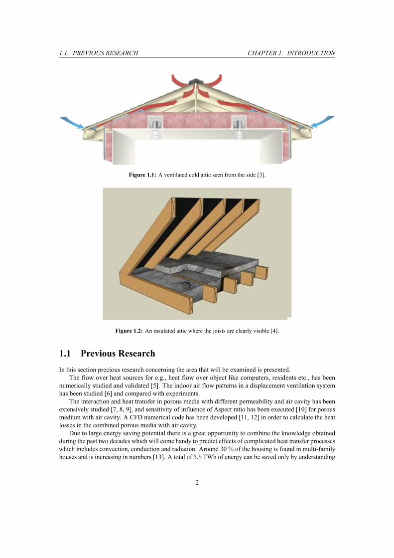
The principal design of a cold attic can be seen in Figure 1.1. The attic consists of a horizontal layer of

insulation with an overlying air cavity. The roof itself does not contain any insulation. The arrows in the

figure indicates attic ventilation, where air flows into the attic through thin gaps along the sides and out

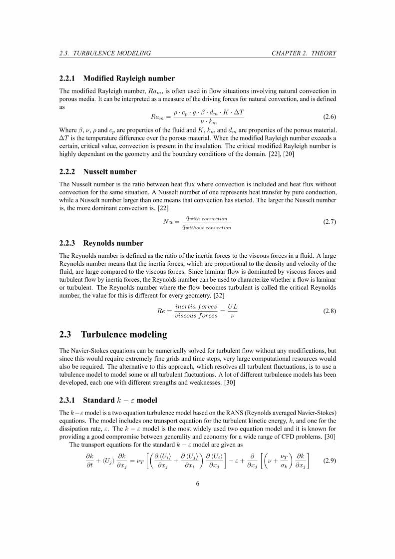
through the ridge. There is a layer of wooden joists laying in a transversal direction on the floor of the

insulation. These can be seen in Figure 1.2.

Modern cold attics are often colder than old ones, due to the increased insulation layer thickness used

nowadays. This can actually lead to serious problems since humid air rising from within the house can

cause mold damages on the roof, the joists, and other wooden based material used in the attic [2]. The air

flow rate that ventilates the attic needs to be dimensioned correctly; since a too high flow of outdoor air into

the attic also can cause problems with humidity, and thus mold. It is clear that a thorough understanding of

the physics governing the heat, air and, moisture for cold attics could help optimizing the design of attics

and thus save energy.

1

1.1. PREVIOUS RESEARCH CHAPTER 1. INTRODUCTION

Figure 1.1: A ventilated cold attic seen from the side [3].

Figure 1.2: An insulated attic where the joists are clearly visible [4].

1.1 Previous Research

In this section precious research concerning the area that will be examined is presented.

The flow over heat sources for e.g., heat flow over object like computers, residents etc., has been

numerically studied and validated [5]. The indoor air flow patterns in a displacement ventilation system

has been studied [6] and compared with experiments.

The interaction and heat transfer in porous media with different permeability and air cavity has been

extensively studied [7, 8, 9], and sensitivity of influence of Aspect ratio has been executed [10] for porous

medium with air cavity. A CFD numerical code has been developed [11, 12] in order to calculate the heat

losses in the combined porous media with air cavity.

Due to large energy saving potential there is a great opportunity to combine the knowledge obtained

during the past two decades which will come handy to predict effects of complicated heat transfer processes

which includes convection, conduction and radiation. Around 30 % of the housing is found in multi-family

houses and is increasing in numbers [13]. A total of 3.5TWh of energy can be saved only by understanding

2

1.2. PURPOSE CHAPTER 1. INTRODUCTION

the process of heat transfer and by implementing proper thermal design [14].

[15, 16, 17] and [18, 19] have published experimental results obtained on the large-scale facilities.

[15] showed that there was an insignificant reduction in thermal resistance due to convection, but the

measurement was conduction at lowmodified Rayleigh number (less permeable products and low velocities).

[17] study was more permeable and thermally conductive products and showed that heat transfer due to

convection, at very low outside temperatures, leading to 50 % reduction in thermal resistance in porous

materials inside attics.

[19] concluded that the heat transfer due to natural convection starts with the modified Rayleigh

numbers from 22 to 27. [19] also showed that the thermal resistance decreases by 25 % when the modified

Rayleigh number is 34. [20] and [21] have carried out similar experiments in small scale test facilities.

[20], [22] and [19] have used a simple computer program to calculate the heat transport only within the

porous medium and the solid inclusions. The effect of air movement in the wind was calculated using a

fictitious thermal resistance at the upper surface of the porous medium.

A 2D calculation based on CFD described in [23], was based on the numerical integration of the

equation for the balance of mass, momentum and energy, both in the porous medium (with the solids

inclusions) and in the air gap. During this investigation a very simplified geometry, with respect to that of

an actual attic was implemented.

When the design of the building envelope changes, especially with regards to thermal insulation and air

tightness, the complex heat transfer processes are often neglected and the same are an important parameter

that influences thermal efficiency and comfort of buildings. [24] has studied the effect of the natural

convective flow and heat transfer between the air gap and a porous medium inside a rectangular space.

[25] studied the effect of natural convection in a vertical porous path to an internal heat source. [26], has

investigated the effect of natural convection in a vertical porous wall which took into account the Brinkman

and Darcy formulations.

[27] has analyzed the effects of displacement ventilation in a three dimensional space. The airflow

over the heat sources, such as heat flow of items such as computers, accommodation, etc., have been

numerically studied and validated by [28], [29] and [5]. Air flow patterns in a ventilation system has been

studied [6] and compared with experiments.

1.2 Purpose

So far, the basic research has been performed either by using 2D models, simpler modeling techniques or

fictitious boundary conditions.

In this project, the 3D CFD solver ANSYS Fluent, together with a suitable turbulence model and

radiation model will be applied in order to numerically investigate the air and heat flow in an insulated

cold attic model. The knowledge obtained can then be used in the design of the future environmentally

friendly and energy efficient attics for future sustainable development.

ANSYS Fluent is a widely used CFD software with a lot of different applications, however, it is not as

commonly used in building physics simulations. Because of this, it would be of interest to investigate how

it performs in problems involving for example heat transfer in porous media.

The effect of changing temperature differences across the model will be investigated, along with the

effect of altering the permeability of the insulation and the rate of air displacement that ventilates the attic.

In order to validate the results, simulations will first be performed on a smaller cuboid shaped model, partly

containing insulation. These results will be compared with earlier experimental results from a PhD thesis

by Mihail Serkitjis to assure that the flow, heat transfer and insulation is modeled correctly [20].

The results of the simulations will be mainly presented in three different articles, which are included as

appendices in the thesis. A summary of the results from these articles can be found in Section 4.

3

1.3. LIMITATIONS CHAPTER 1. INTRODUCTION

1.3 Limitations

The main limitation of the project was the time limit, due to the study being part of a master thesis. This

forced the project to be executed during a period of approximately eighteen weeks. Because of this, no

transient simulations were performed. Furthermore, only the heat transfer and flow fields of the simulations

were investigated, while more advanced phenomena such as moisture transport was not included.

The simulations have been performed using Fluent as the only CFD solver, and the mesh size has been

restricted to 512000 computational cells due to only an academic license of Fluent being available.

4

CHAPTER 2. THEORY

2 Theory

This chapter includes brief descriptions of the relevant equations, dimensionless numbers and other

theoretical concepts used in this thesis.

2.1 Governing equations

The following equations are used in order to mathematically describe fluid flow.

2.1.1 Continuity equation

This is the three dimensional and unsteady continuity equation for a compressible fluid. The first term

describes the rate of change in time of the density and the second term describes the net flow of mass out

of the element boundaries. [30]∂ρ

∂t+

∂ρUj

∂xj= 0 (2.1)

2.1.2 Momentum equation

This is the momentum equation, or Navier Stokes equation, written in tensor notation. The momentum

equation is obtained by applying Newton’s second law to a fluid particle. [30]

∂Ui

∂t+ Uj

∂Ui

∂xj= −1

ρ

∂p

∂xi+

1

ρ

∂τji∂xj

+ gi (2.2)

2.1.3 Energy equation

The energy equation [31] for incompressible flow with constant cp reads:

ρdu

dt= −p

∂Ui

∂xi+Φ+

∂

∂xi

(k∂T

∂xi

)(2.3)

where Φ is defined as:

2µSijSij −2

3µSiiSkk (2.4)

and Sij is the strain-rate tensor:

Sij =1

2

(∂Ui

∂xj+

∂Uj

∂xi

)(2.5)

2.2 Dimensionless numbers

In this section the relevant dimensionless numbers are described.

5

2.3. TURBULENCE MODELING CHAPTER 2. THEORY

2.2.1 Modified Rayleigh number

The modified Rayleigh number, Ram, is often used in flow situations involving natural convection in

porous media. It can be interpreted as a measure of the driving forces for natural convection, and is defined

as

Ram =ρ · cp · g · β · dm ·K ·∆T

ν · km(2.6)

Where β, ν, ρ and cp are properties of the fluid andK, km and dm are properties of the porous material.

∆T is the temperature difference over the porous material. When the modified Rayleigh number exceeds a

certain, critical value, convection is present in the insulation. The critical modified Rayleigh number is

highly dependant on the geometry and the boundary conditions of the domain. [22], [20]

2.2.2 Nusselt number

The Nusselt number is the ratio between heat flux where convection is included and heat flux without

convection for the same situation. A Nusselt number of one represents heat transfer by pure conduction,

while a Nusselt number larger than one means that convection has started. The larger the Nusselt number

is, the more dominant convection is. [22]

Nu =qwith convection

qwithout convection(2.7)

2.2.3 Reynolds number

The Reynolds number is defined as the ratio of the inertia forces to the viscous forces in a fluid. A large

Reynolds number means that the inertia forces, which are proportional to the density and velocity of the

fluid, are large compared to the viscous forces. Since laminar flow is dominated by viscous forces and

turbulent flow by inertia forces, the Reynolds number can be used to characterize whether a flow is laminar

or turbulent. The Reynolds number where the flow becomes turbulent is called the critical Reynolds

number, the value for this is different for every geometry. [32]

Re =inertia forces

viscous forces=

UL

ν(2.8)

2.3 Turbulence modeling

The Navier-Stokes equations can be numerically solved for turbulent flow without any modifications, but

since this would require extremely fine grids and time steps, very large computational resources would

also be required. The alternative to this approach, which resolves all turbulent fluctuations, is to use a

tubulence model to model some or all turbulent fluctuations. A lot of different turbulence models has been

developed, each one with different strengths and weaknesses. [30]

2.3.1 Standard k − ε model

The k−εmodel is a two equation turbulence model based on the RANS (Reynolds averaged Navier-Stokes)equations. The model includes one transport equation for the turbulent kinetic energy, k, and one for thedissipation rate, ε. The k − ε model is the most widely used two equation model and it is known forproviding a good compromise between generality and economy for a wide range of CFD problems. [30]

The transport equations for the standard k − ε model are given as

∂k

∂t+ 〈Uj〉

∂k

∂xj= νT

[(∂ 〈Ui〉∂xj

+∂ 〈Uj〉∂xi

)∂ 〈Ui〉∂xj

]− ε+

∂

∂xj

[(ν +

νTσk

)∂k

∂xj

](2.9)

6

2.4. THE BOUSSINESQ MODEL CHAPTER 2. THEORY

∂ε

∂t+ 〈Uj〉

∂ε

∂xj= Cε1νT

ε

k

[(∂ 〈Ui〉∂xj

+∂ 〈Uj〉∂xi

)∂ 〈Ui〉∂xj

]−Cε2

ε2

k+

∂

∂xj

[(ν +

νTσε

)∂ε

∂xj

](2.10)

Where νT is the turbulent viscosity, calculated as

νT = Cµk2

ε(2.11)

The values of the constants in the model are given below in table 2.1. [30]

Table 2.1: Constants for the k − ε model

Constant Value

Cµ 0.09

Cε1 1.44

Cε2 1.92

σk 1.00

σε 1.30

2.3.2 Modified k − ε model

The realizable k − ε model is a modification of the standard k − ε model. In this model the parameterCµ is a function of the local state of the flow, rather than being a constant value. This approach ensures

that the normal stresses are positive under all possible flow conditions. In addition, the realizable k − εmodel generally includes a production term for dissipation of turbulent energy dissipation in the ε equation.Previous research has proven the realizable k− εmodel superior over the standard k− εmodel in complexflow situations, e.g. boundary layer flow, separated flows and rotating shear flows. The transport equations

for the realizable k − ε model are the same as for the standard model. [30]

2.4 The Boussinesq model

The Boussinesq model is an approximation often used in buoyancy driven natural convection flows. In

this model, the density is constant in all solved equations except for the buoyancy term in the momentum

equation. Here ρ0 is the constant density of the flow, T0 is the operating temperature and β is the thermal

expansion coefficient. The Boussinesq model is a good approximation as long as the temperature difference

in the domain is not too large. [33]

(ρ− ρ0) ≈ −ρ0β(T − T0) (2.12)

2.5 Mechanisms of heat transfer

Heat can be transfered in three different ways: conduction, convection and radiation. A temperature

difference is required for all this modes of heat transfer to take place, and the heat always transfers from

regions of high temperature to regions of lower. [32]

7

2.6. BOUNDARY CONDITIONS CHAPTER 2. THEORY

2.5.1 Conduction

Conduction is the transfer of heat as a result of interactions between particles. Conduction can occur in

solids, fluids and gases. In gases and fluids, conduction is caused by collisions and diffusion of molecules

during their random motion. In solids it is caused by vibrations of molecules in a lattice and the energy

transport of free electrons. Steady one dimensional heat conduction is defined as

Qconduction = −kAdT

dx(2.13)

which is also known as Fourier's law. Here A is the heat transfer surface area, which is always normal to

the direction of heat transfer, and k is the thermal conductivity of the material. [32]

2.5.2 Convection

Convective heat transfer takes place in fluids in the presence of fluid motion. Convective heat transfer is

divided into natural and forced convection. In forced convection the fluid motion is initiated externally,

e.g. by a fan or a pump, while in natural convection it is caused by density differences in the fluid due to

temperature gradients. Convective heat transfer from a solid surface to the surrounding fluid is defined as

Qconvection = hA(Ts − T∞) (2.14)

which is known as Newton's law of cooling. Here h is the convection heat transfer coefficient, A is the heat

transfer surface area, Ts is the temperature of the surface and T∞ is the temperature of the fluid sufficiently

far away from the surface. [32]

2.5.3 Radiation

Radiation is a process where energy is emitted by matter in the form of electromagnetic waves. Radiation

does not, unlike conduction and convection, require a medium in order to transfer energy, it works just

as well in vacuum. The relevant type of radiation for heat transfer studies is thermal radiation, which is

emitted by all bodies at a temperature over absolute zero. The net radiative heat transfer is calculated as

Qradiation = εσA(T 4s − T 4

surr) (2.15)

where ε, A and Ts is the emissivity, surface area and absolute temperature, respectively, of a body and

Tsurr is the absolute temperature of the surrounding surface. The Stefan-Boltzmann constant, σ, is equalto 5.67 · 10−8W/(m2 ·K4). [32]

2.6 Boundary Conditions

The thermal boundary conditions used in this thesis work were prescribed temperature (Dirichlet):

T = Tw (2.16)

and prescribed heat flux (Neumann):

k∂T

∂n= −qw (2.17)

where the subscript w indicates wall. When the heat flux is prescribed to be zero, the boundary condition

is called adiabatic. This simulates a perfectly insulated boundary.

8

2.7. MODELING OF FLUID FLOW IN POROUS MEDIA CHAPTER 2. THEORY

2.7 Modeling of fluid flow in porous media

The following section provides information about the relevant concepts and equations regarding fluid flow

in porous media.

2.7.1 Porosity

The porosity, or void fraction, of a porous medium is defined as the fraction of the total volume that is

occupied by voids. For a porous medium with porosity ϕ, the volume occupied by solid material is thus1− ϕ. [34]

2.7.2 Darcy's law and Permeability

Darcy's law is an empirically derived and well verified formula which relates the flow velocity and pressure

difference in a porous medium. Darcy's law is defined as

u = −K

µ

∂P

∂x(2.18)

which, for an isotropic medium, can be simplified and rewritten as

∇P = − µ

Kv (2.19)

where µ is the dynamic viscosity of the fluid andK is the permeability of the medium. The permeability

can be seen as a measure of the ability for a fluid to pass through the porous medium, where a higher

permeability implies that more fluid is transported through it. The value of the permeability depends on

the geometry of the medium and has the dimension of (length)2. [34]

Several extensions to Darcy's law has been made over time, e.g Forchheimers equation, Brinkman’s

equation etc. [34]

2.7.3 Porous media in Fluent

Porous media are modeled in Fluent as an extra momentum source term to the standard fluid flow equations.

The source term consists of two terms: the first one is due to viscous losses, according to Darcy's law, and

the second one is due to inertial losses.

Si =

(µ

Kvi + C2

1

2ρ |v| vi

)(2.20)

K is here the permeability of the porous media and C2 is the inertial resistance factor. For laminar flows

in porous media, the viscous losses are dominant and C2 can be consdiered to be zero. The porous media

model then reduces to Darcy's law. On the other hand, at high flow velocities C2 provides a correction for

inertial losses in the porous medium. [33]

2.8 Radiative heat transfer in Fluent

The P-1 radiation model [33] was used for both the two and three dimensional simulations. For modeling

gray radiation, the following equation describes the radiation heat flux qr:

qr = − 1

3 (a+ σs)− Cσs∇G (2.21)

9

2.8. RADIATIVE HEAT TRANSFER IN FLUENT CHAPTER 2. THEORY

where a is the absorption coefficient, σs the scattering coefficient, G is the incident radiation and C is the

linear-anisotropic phase function coefficient. The transport equation for G is:

∇ · (Γ∇G)− aG+ 4an2σT 4 = SG (2.22)

where Γ is defined as:

Γ =1

3 (a+ σs)− Cσs(2.23)

10

CHAPTER 3. METHOD

3 Method

In this chapter the methodology used while setting up and running the simulations is discussed.

3.1 Software

In order to both create the different geometries and the meshes used for the different cases, ANSYS

ICEM CFD, hereby referred to as Icem, was used. It is a commercial software able to create advanced

user-specified geometries and computational grids.

The simulations were performed using the CFD solver ANSYS Fluent, hereby referred to as Fluent. It

is a widely used powerful CFD software used for a broad range of purposes. It was also used for a large

part of the postprocessing and visualization of the results.

For further postprocessing and calculation of relevant flow variables, MATLAB was used.

3.2 Geometry

3.2.1 Insulation Box

As mentioned in Section 1.2, initial simulations was performed on a smaller model named the insulation

box, with dimensions set to imitate one of the cases in [20]. The insulation box model was created in both

2D and 3D. This basic model consists of a cuboid, filled with insulation in its lower part. The model is

visually presented and the consisting parts are described in Figure 3.1 and Table 3.1 respectively. The

dimensions of the insulation box can be found in Figure 3.2 combined with Table 3.2. Note that the depth

of the model is 0.6m. As mentioned in the previous section, the geometries were both created in Icem.

Table 3.1: Description of Figure 3.1

A Side Walls

B Floor

C Top Edge of Insulation

D Back/Front Walls

E Roof

Table 3.2: Description of Figure 3.2

a 0.2 m

b 0.3 m

c 0.8 m

11

3.2. GEOMETRY CHAPTER 3. METHOD

Figure 3.1: Overview of the Insulation Box model.

Figure 3.2: Front view of the Insulation Box.

3.2.2 Attic Model

The attic model was created to mimic the normal conditions for a cold attic as close as possible, while

still retaining a rather simple approach in order to be able to satisfy the constraints regarding the mesh

size. These constraints will be discussed further in the following paragraph, section 3.3. The attic model

consists of an insulation layer on the bottom as in the insulation box, and an air layer above it shaped like a

generic attic. In order to help with the mesh constraint, only a part of the length of the attic was included in

the model, along with appropriate boundary conditions on the walls where it was cut off. More information

on these boundary conditions can be found in section 3.4.2.

The attic model includes two inlets and an outlet to be able to simulate a ventilation system. The inlets

are placed at either side of the model, and leads in air through a small passage between the roof and the

wind deflectors, which guides the flow in the correct direction and stops the inlet flow from entering the

insulation directly. The air then flows out through the top of the roof through an outlet that is made to

simulate a ridge ventilation system, which is one of the more common ways to design an attic ventilation

system [3, 35]. Furthermore, several joists are lined up along the floor of the model, perpendicular to the

side walls and stretching through the whole length between the same. Joists are very common in cold attics,

12

3.2. GEOMETRY CHAPTER 3. METHOD

and due to the high thermal conductivity of the wooden material they are made of, they will influence the

convection process.

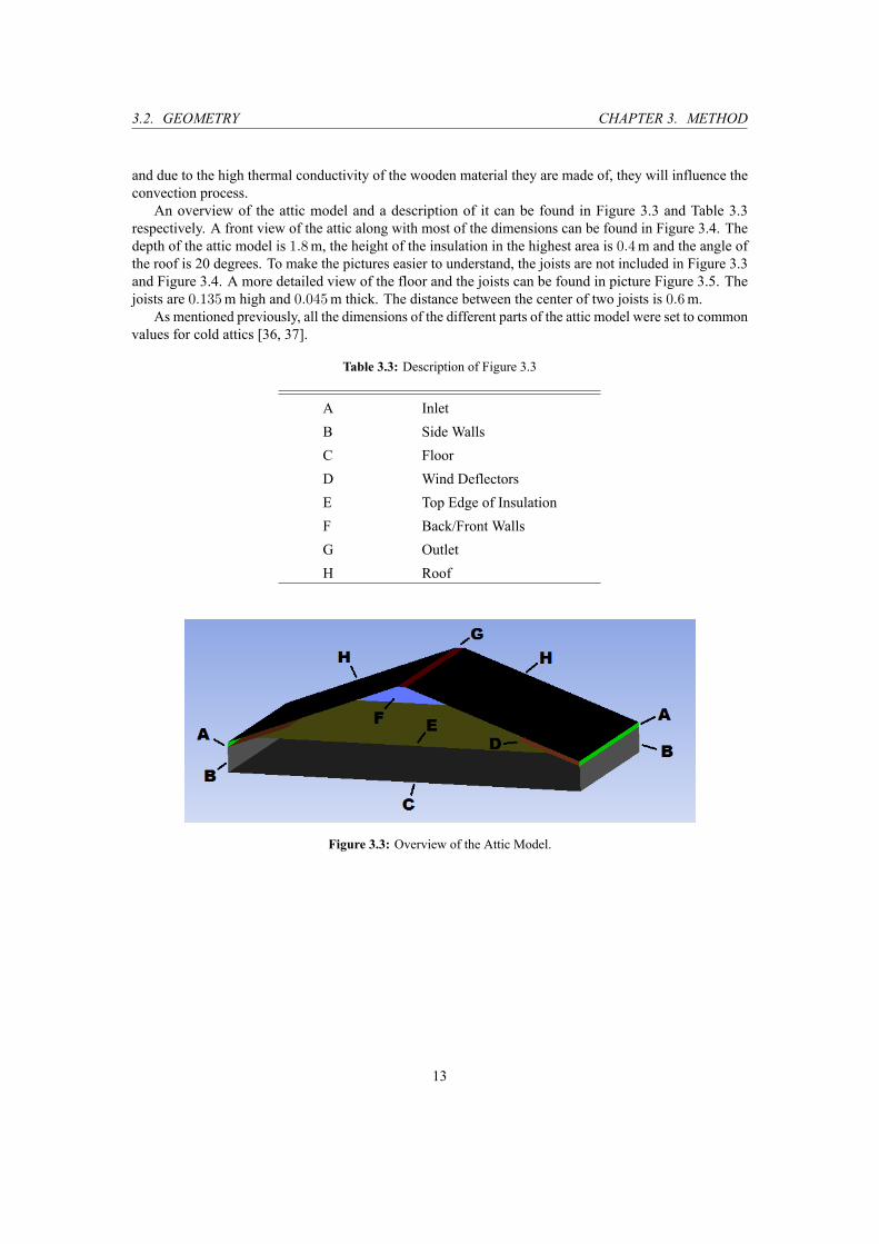
An overview of the attic model and a description of it can be found in Figure 3.3 and Table 3.3

respectively. A front view of the attic along with most of the dimensions can be found in Figure 3.4. The

depth of the attic model is 1.8m, the height of the insulation in the highest area is 0.4m and the angle of

the roof is 20 degrees. To make the pictures easier to understand, the joists are not included in Figure 3.3

and Figure 3.4. A more detailed view of the floor and the joists can be found in picture Figure 3.5. The

joists are 0.135m high and 0.045m thick. The distance between the center of two joists is 0.6m.As mentioned previously, all the dimensions of the different parts of the attic model were set to common

values for cold attics [36, 37].

Table 3.3: Description of Figure 3.3

A Inlet

B Side Walls

C Floor

D Wind Deflectors

E Top Edge of Insulation

F Back/Front Walls

G Outlet

H Roof

Figure 3.3: Overview of the Attic Model.

13

3.3. MESH CHAPTER 3. METHOD

Figure 3.4: Front view of the Attic Model. The upper region represents the air cavity and the lower one the

porous insulation.

Figure 3.5: View of the joists at the floor of the insulation.

3.3 Mesh

After creating the geometries in Icem, the meshes for the different models were created. All the meshes

contain only hexahedral cells, and were created using the blocking method in Icem. This method involves

creating a number of blocks which each contain a specified amount of computational cells. The combined

volumes of these blocks make up the geometry that is supposed to be meshed.

The main concern when creating the meshes was to keep the amount of cells for a particular geometry

below 512000. This is a constraint that the academic license version of Fluent has, and which had to be

respected because of the lack of access to a full Fluent license during the project. Because of this constraint,

the ability to optimize the meshes was severely reduced, especially for the attic model case. Information

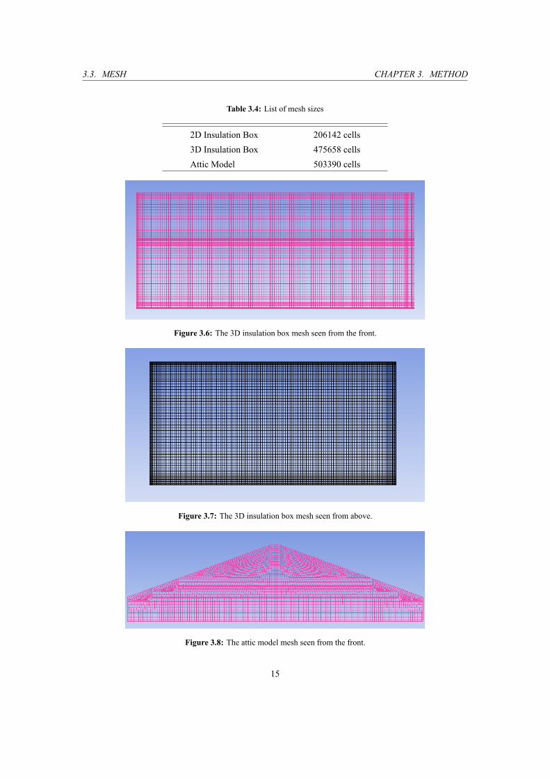
regarding the size of the different meshes can be found in Table 3.4. Pictures of the 3D insulation box

mesh can be seen in Figure 3.6 and Figure 3.7. Note that the 2D mesh for the insulation box is constructed

in the exact same way as the front view of the 3D version in Figure 3.6, but denser. The mesh for the attic

model is presented in Figure 3.8 and Figure 3.9.

14

3.3. MESH CHAPTER 3. METHOD

Table 3.4: List of mesh sizes

2D Insulation Box 206142 cells

3D Insulation Box 475658 cells

Attic Model 503390 cells

Figure 3.6: The 3D insulation box mesh seen from the front.

Figure 3.7: The 3D insulation box mesh seen from above.

Figure 3.8: The attic model mesh seen from the front.

15

3.3. MESH CHAPTER 3. METHOD

Figure 3.9: The attic model mesh seen from above.

16

3.4. FLUENT SETTINGS CHAPTER 3. METHOD

3.4 Fluent Settings

As with all CFD software, there is a large amount of settings available for adjustment in Fluent to get the

desired simulation. A summary for the most relevant settings for the simulations ran during this project

can be found in Table 3.5 below. In addition to this, Least Squares Cell Based discretization was used to

calculate the gradients in the cell centers, Body Forced Weighted discretization was used for the pressure,

and Second Order Upwind was used for momentum, k, ε and energy.

Table 3.5: General Fluent Settings

Time Dependency Steady

Solver Type Pressure-Based

Turbulence Model Realizable k − ε model

Radiation Model P1

Pressure-Velocity Scheme SIMPLEC

3.4.1 Modeling the Insulation

In order to simulate the insulation, the cell zone containing the insulation was set as a so called porous zone

in Fluent. As mentioned in Section 2.7.3, Fluent simulates the porous zone by adding an extra momentum

equation to the flow equations for the particular zone. It is possible to specify the resistance coefficients

for this equation along with the thermal conductivity for the cell zone in order to simulate the desired

insulation properties.

The main problem with Fluent's way of modelling porous media is that it is only possible to add a

resistance to the conductive and convective heat transfer in the insulation area, and not the heat transfer by

radiation [33, 39]. Fluent sees the insulation zone as a volume filled with air but with changed properties

regarding conduction and resistance to fluid flow. Thus, the insulation zone does not involve any actual

solid parts which can reduce the radiative heat transfer. This causes the total heat flow through the insulation

to be overpredicted which is a very important aspect to keep in mind when considering the results of the

simulations performed during this work.

The permeability used for the insulation in the insulation box was 5 · 10−8m2 in order to be able to

compare and validate the results with those with the same permeability from Serkjitis thesis.The insulation

was simulated in the same way for the attic model as for the insulation box case. However, besides the

permeability of 5 · 10−8m2 that was used for the insulation box, simulations were also performed with an

insulation permeability of 4·10−8m2. This was done in order to be able to investigate the effects of a change

in permeability of the insulation. The thermal conductivity of the insulation was set to 0.044W/(m · K)for all of the cases. This choice of thermal conductivity is not entirely physical, since in reality the thermal

conductivity changes with changing mean temperature of the insulation. Despite this, the approximation

was done first and foremost since this was the thermal conductivity in the experiments by Serkjitis that

were used for validation. Furthermore, the difference in mean temperature of the insulation between the

simulations of the cases presented in this thesis is small enough that the thermal conductivity is not majorly

affected.

Worth noting is that the insulation volume is specified as a laminar zone. This suppresses the effect of

turbulence in the area by setting the turbulent contribution to viscosity to zero. Fluent suggests using this

setting for porous media as long as the permeability of the medium is not too large [39]. This was also

tested by running several simulations without this option enabled for the insulation, which all produced

very unphysical results.

17

3.4. FLUENT SETTINGS CHAPTER 3. METHOD

3.4.2 Boundary Conditions

Along with the general solver settings in Fluent, the boundary conditions must also be set correctly to get a

satisfactory simulation.

Insulation Box

For the insulation box cases, a Neumann temperature boundary condition was specified on all the sides of

the box, with the temperature gradient set to zero. The floor boundary condition was set to a Dirichlet

temperature boundary condition with a specified temperature of 294K, simulating the temperature of theroof of a room with normal indoor climate. A Dirichlet temperature boundary condition was also specified

on the roof of the insulation box. The specified temperature on this boundary was changed between each

case to achieve simulations with a temperature difference across the box ranging from 10 to 50K.This method is somewhat different to the method Serkjitis used in his work. In his experiments, the

mean temperature in the insulation was kept constant throughout all temperature differences. This was

achieved by changing both the high and the low temperatures on the box.

A summary of the boundary conditions for the insulation box can be found in Table 3.6 below.

Table 3.6: Insulation Box Boundary Conditions

Floor Dirichlet, T = 294K

Roof Dirichlet, T = 294 –∆T K

Walls Neumann, dT /dx = 0

Attic Model

As mentioned above, in order to simulate the attic model as a part of a larger attic, an appropriate boundary

condition is needed for the sides that separates the model from the rest of the attic. To achieve this, a

symmetry boundary condition was used for these sides in the attic model.

For the rest of the model, a Neumann temperature boundary condition with the temperature gradient

set to zero was used for the other walls connected to the insulation. This is an approximation, since in

reality these walls are in contact with the outside. A more appropriate boundary condition would therefore

be a Dirichlet condition with specified outside temperature. This approximation was made because the

simulations were found to be faster and more stable in this case, while it also was assumed to make a rather

small difference.

The wind deflectors are both set as a shell conduction boundary, with the material data of plywood.

This setting means that conduction is allowed through the solid wind deflectors. As in the insulation box

case, the floor is set to a Dirichlet temperature boundary condition with the specified temperature of 294K.For the cases involving solely natural convection, the inlet, outlet and the roof are all set as walls with

a Dirichlet temperature boundary condition that varies between cases to achieve different temperature

differences, as for the insulation box simulations. For the cases that investigate forced convection, the

inlet boundaries are set as velocity inlets. The effects of three different inlet velocities were investigated,

each corresponding to a certain rate of complete air displacement in the attic. The inlet velocities were

0.0113m/s, 0.0226m/s and 0.0452m/s, which correspond to 2, 4 and 8 complete air displacements perhour, respectively. The outlet boundary was in these cases set to a pressure outlet with the same pressure

as inside the attic, i.e. atmospheric pressure, in order to get a natural outflow. The boundary conditions

specified for the attic model can be found in Table 3.7.

18

3.5. RUNNING THE SIMULATIONS CHAPTER 3. METHOD

Table 3.7: Attic Model Boundary Conditions

Floor Dirichlet, T = 294K

Roof Dirichlet, T = 294 –∆T K

Back/Front Walls Symmetry

Side Walls Neumann, dT /dx = 0

Inlet (Natural Convection Cases) Dirichlet, T = 294 –∆T K

Inlet (Forced Convection Cases) Velocity Inlet, v = 0.0113 - 0.0452m/s

Outlet (Natural Convection Cases) Dirichlet, T = 294 –∆T K

Outlet (Forced Convection Cases) Pressure Outlet, P = Atmospheric Pressure

Wind Deflectors Shell Conduction

3.5 Running the Simulations

In order to run the rather large amount of simulations smoothly, the simulations were run on the computer

cluster Glenn. Glenn is a part of Chalmers Centre for Computational Science and Engineering [38].

Since all of the simulations are steady state cases, the simulations were not run a certain amount of

time or time steps, but rather until a stable solution was reached.

In order to ensure these stable converged solutions, the residuals of the simulations were monitored

until they reached a stable low enough level. In the forced convection cases the total net mass flow was

also monitored to ensure that global mass continuity was satisfied.

19

CHAPTER 4. RESULTS

4 Results

The results from this thesis work are mainly presented in the three papers that are attached in the end of

this thesis. In this section a short summary of the results of each of the papers is presented.

4.1 Paper 1: Influence of Heat Transfer Processes in Porous Media

with Air Cavity - A CFD Analysis

The calculated modified Rayleigh and Nusselt numbers from both the 2D and 3D simulations of the

insulation box, compared with the results from the same case by Serkitjis can be found in Figure 4.1 below.

The figure shows results from simulations both with and without radiation.

0 10 20 30 40 501

1.2

1.4

1.6

1.8

2

2.2

Ram

Nu

Experiments

2D Case With Radiation

3D Case With Radiation

2D Case Without Radiation

3D Case Without Radiation

Figure 4.1: Plot of the Nusselt number versus the modified Rayleigh number for the 2D case (blue line), the 3D

case (green line) and the values obtained by the experimental work [20] (red line).

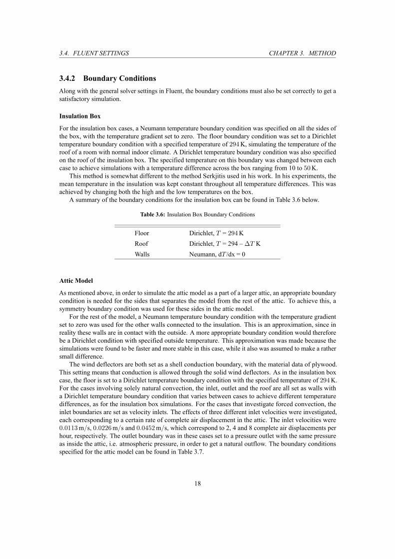
Temperature profiles from a selection of the 3D simulations can be found in Figure 4.2. The figure

shows how the temperature profiles evolve with increasing temperature difference. The 2D simulations

showed a similar pattern of development.

The flow profile of the 3D case with a temperature difference of 30K is presented in Figure 4.3. It can

be noted from this figure that two distinct convection cells are formed in the air cavity. These penetrate

the insulation and cause a downward motion in the middle of the insulation, and an upward motion at

the edges. This flow pattern was identified in all of the simulations, both in 2D and 3D. However, the

magnitude of the velocity increased with increasing temperature difference.

This flow pattern phenomenon explains the shape of the temperature profiles, where the center of the

insulation has a lower temperature since cold air flows down in that area, and the edges of the insulation has

a higher temperature where the hot air flows upwards. This phenomenon can also be seen in the horizontal

view inside the insulation in Figure 4.4.

20

4.1. PAPER 1 CHAPTER 4. RESULTS

Figure 4.2: Temperature contours for the 3D case for, in order from above, 10, 30 and 50K temperature

difference.

21

4.1. PAPER 1 CHAPTER 4. RESULTS

Figure 4.3: Velocity vectors for the 3D case with a temperature difference of 30K. The first picture from above

is flow in the air cavity and the second one is flow in the insulation. The arrows indicate the direction of the flow.

Figure 4.4: Temperature contours taken in a horizontal plane in the middle of the insulation for the three

dimensional case with a temperature difference of 30 K.

22

4.2. PAPER 2 CHAPTER 4. RESULTS

4.2 Paper 2: Numerical Analysis of the Influence of Natural Con-

vection in Attics

The Nusselt number versus the modified Rayleigh number for the simulations included in Paper 2 can be

found in Figure 4.5.

0 10 20 30 40 501

1.1

1.2

1.3

1.4

1.5

Ram

Nu

K = 5 ⋅ 10−8

K = 4 ⋅ 10−8

Figure 4.5: The Nusselt number versus the modified Rayleigh number for the attic model case with natural

convection.

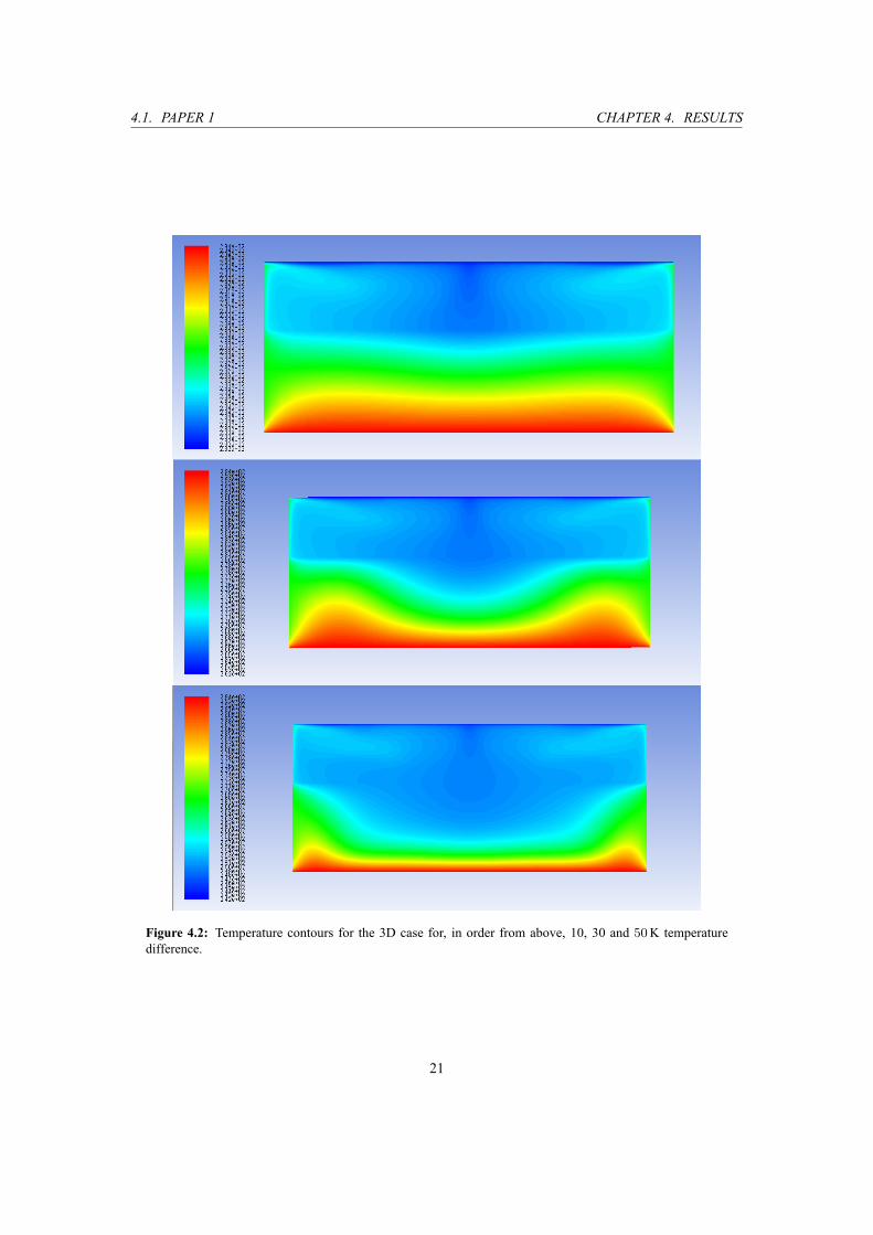
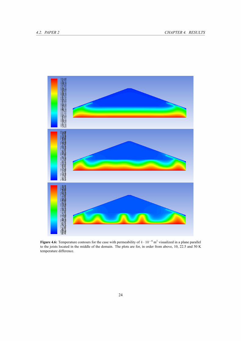
In Figure 4.6 and Figure 4.7, some of the temperature profiles for the simulations of the attic involving

only natural convection, for both permeabilities, can be found. It can be seen that the development of the

temperature contours does not follow any pattern, but is rather chaotic. The only simulations with a clear

pattern are the ones with the lowest temperature difference, which is due to convection not having started

yet in these simulations.

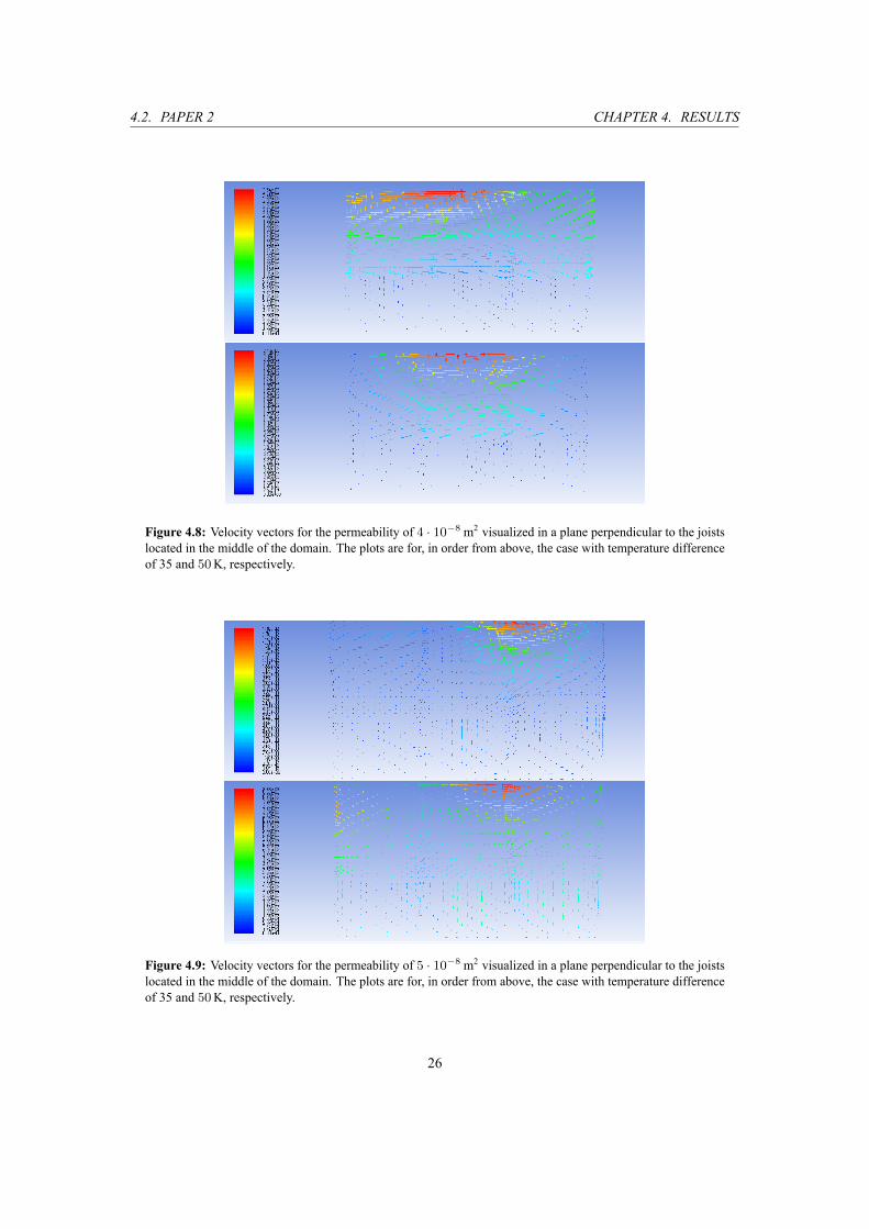
When inspecting the flow seen in a plane perpendicular to the joists for the temperature differences of

35K and 50K for both permeabilities, Figure 4.8 and Figure 4.9, it is possible to note that the air seems

to flow in a large cylindrical convection cell across this dimension of the domain. The unsteady nature

of natural convection can also be noted when inspecting Figure 4.8. After an increase in temperature

difference of 15K, the flow creating this large convection cell has changed direction.

The impact of the joists can be seen in Figure 4.10. The joists are expected to accelerate the flow

upwards along them since they have a higher thermal conductivity than the insulation. However, this is

only the case for some of the joists in this picture, which is most likely due to the overall heat flow through

the attic which forces the air to flow down around the joists in some parts of the domain.

23

4.2. PAPER 2 CHAPTER 4. RESULTS

Figure 4.6: Temperature contours for the case with permeability of 4 · 10−8 m2 visualized in a plane parallel

to the joists located in the middle of the domain. The plots are for, in order from above, 10, 22.5 and 50 K

temperature difference.

24

4.2. PAPER 2 CHAPTER 4. RESULTS

Figure 4.7: Temperature contours for the case with permeability of 5 · 10−8 m2 visualized in a plane parallel

to the joists located in the middle of the domain. The plots are for, in order from above, 10, 22.5 and 50 K

temperature difference.

25

4.2. PAPER 2 CHAPTER 4. RESULTS

Figure 4.8: Velocity vectors for the permeability of 4 · 10−8 m2 visualized in a plane perpendicular to the joists

located in the middle of the domain. The plots are for, in order from above, the case with temperature difference

of 35 and 50K, respectively.

Figure 4.9: Velocity vectors for the permeability of 5 · 10−8 m2 visualized in a plane perpendicular to the joists

located in the middle of the domain. The plots are for, in order from above, the case with temperature difference

of 35 and 50K, respectively.

26

4.2. PAPER 2 CHAPTER 4. RESULTS

Figure 4.10: Velocity vectors scaled to show the velocities in the insulation for the temperature difference of

40K and permeability of 4 · 10−8 m2. The figure is visualized in a plane perpendicular to the joists located in

the middle of the domain.

27

4.3. PAPER 3 CHAPTER 4. RESULTS

4.3 Paper 3: CFD Analysis of Heat Transfer in Ventilated Attics

The Nusselt number versus the modified Rayleigh number for the simulations included in Paper 3 can

be found in Figure 4.11. A more detailed view of the differences in Nusselt number results between the

different air displacement rates for some temperature differences can be found in Figure 4.12 for the

permeability of 4 · 10−8m2 and Figure 4.13 for the permeability of 5 · 10−8m2.

0 10 20 30 40 501

1.1

1.2

1.3

1.4

1.5

Ram

Nutot

K5 With L2

K5 With L4

K5 With L8

K4 With L2

K4 With L4

K4 With L8

Figure 4.11: Plot of The Nusselt number versus the modified Rayleigh number for the cases with permeability

of 4 · 10−8 m2 (the three dashed lines) and the cases with permeability of 5 · 10−8 m2 (the three solid lines). L2,

L4 and L8 represent two, four and eight complete air displacements per hour, respectively.

As for the simulations conducted for the attic model including only natural convection, the temperature

profiles for the attic model with the added ventilation system are very chaotic and irregular. There are also

no patterns in development between different temperature differences or air displacement rates. A view of

the difference between air displacement rates for the temperature difference of 35K and the permeability

of 4 · 10−8m2 can be seen in Figure 4.14.

The velocity vectors for the temperature difference of 35K and the permeability of 4 · 10−8m2 is

visualized in Figure 4.15 for two different complete air displacement rates. The air movements in the

air cavity are fairly structured, and the only difference between different displacements rates from this

view is that the velocity of the flow increases in the whole air cavity with increasing displacement rates.

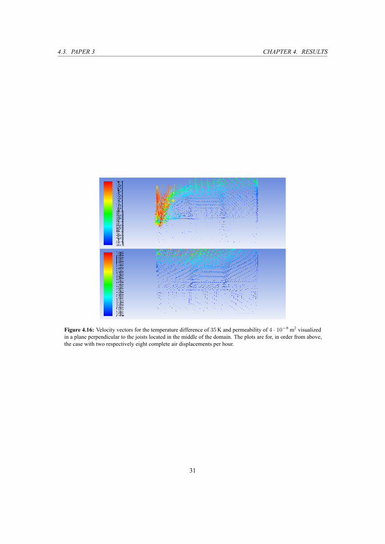
When inspecting the flow in a plane perpendicular to the joists for the same temperature difference and

permeability, Figure 4.16, it can be noted that a swirl is created in the air cavity above the insulation.

However, when the air displacement rate increases, this swirl disappears and the flow seems to become

more structured in the air cavity.

28

4.3. PAPER 3 CHAPTER 4. RESULTS

40 60 80 100 120 140 160 1801

1.05

1.1

1.15

1.2

1.25

1.3

1.35

Re

Nutot

dT = 40

dT = 45

dT = 50

Figure 4.12: Plot of The Nusselt number versus the Reynolds number for the cases with permeability of

4 · 10−8 m2. The Reynolds number is based on the geometry of the inlet. Each line represents one temperature

difference.

40 60 80 100 120 140 160 1801

1.1

1.2

1.3

1.4

1.5

1.6

Re

Nutot

dT = 35

dT = 45

dT = 50

Figure 4.13: Plot of The Nusselt number versus the Reynolds number for the cases with permeability of

5 · 10−8 m2. The Reynolds number is based on the geometry of the inlet. Each line represents one temperature

difference

29

4.3. PAPER 3 CHAPTER 4. RESULTS

Figure 4.14: Temperature contours for the temperature difference of 35K and permeability of 4 · 10−8 m2

visualized in a plane parallel to the joists, located in the middle of the domain. In order from above, the pictures

are for the cases with two respectively eight complete air displacements per hour.

Figure 4.15: Velocity vectors for the temperature difference of 35K and permeability of 4 · 10−8 m2 visualized

in a plane parallel to the joists located in the middle of the domain. The plots are for, in order from above, the

case with two respectively eight complete air displacements per hour.

30

4.3. PAPER 3 CHAPTER 4. RESULTS

Figure 4.16: Velocity vectors for the temperature difference of 35K and permeability of 4 · 10−8 m2 visualized

in a plane perpendicular to the joists located in the middle of the domain. The plots are for, in order from above,

the case with two respectively eight complete air displacements per hour.

31

CHAPTER 5. DISCUSSION AND CONCLUSIONS

5 Discussion and Conclusions

The results from the work presented in the three papers showed that the applied model for simulating

heat transfer and fluid flow in a domain including insulation and an air cavity gives good results for

the investigated cases. The results seem very physical, and the accuracy of the simulations has been

investigated.

In general, Fluent has proved to be a reliable CFD solver concerning the simulations performed in this

thesis work.

One problem with the accuracy of the simulations is however the way Fluent handles radiation through

a porous zone. As discussed earlier in section 3.4.1, Fluent does not account for a resistance to heat transfer

through radiation in the insulation, and thus this part of the total heat transfer is overpredicted.

Furthermore, the results from all of the papers show that the shape of the domain affects the fluid flow

both in the insulation and the air cavity. The shapes of the convection cells in the two mediums affect each

other and also the shape of the temperature profiles in the two zones.

The temperature and flow profiles in the insulation for the simulations of the attic model in Paper 2

and Paper 3 did not show any clear patterns, but were rather quite chaotic and irregular for all cases where

convection had started. It can be concluded that this was due to the geometry of the attic model, but the

chaotic nature of the profiles might also be due to the overprediction of radiative heat transfer inside the

insulation.

The ventilation system added to the attic model in Paper 3 did affect the fluid flow in the attic, however

the largest clear differences occurred in the air cavity. This was most likely due to the placement of the

inlet and outlet, which forced the inlet flow to mainly follow the roof of the air cavity and flow out at the

outlet on the top of the roof, thus not forcing much flow into the insulation. Although, the convective heat

transfer was still affected by the added ventilation system and an increase of inlet velocity. The Nusselt

number for a certain modified Rayleigh number was generally lowered by these effects, but only by a

small margin. It is hard to draw any real conclusions as to why the Nusselt number was affected in this

particular way, however it most likely depends on the geometry of the attic.

The simulations in Paper 2 and Paper 3 suffer from high continuity residuals. However, the rest of the

residuals show good convergence, as does the total mass flux for the forced convection simulations. The

high continuity residuals most likely stems from the number of cells in the mesh. Due to the restriction of

mesh size without a commercial license of Fluent, it was not possible to create and test a larger mesh, and

since the other convergence checks that was performed showed good convergence, the simulations should

be considered sufficiently accurate.

5.1 Future Work

Going forward with this project, in order to achieve a complete virtual model of a cold attic, several steps

needs to be fulfilled. These mainly include, in order:

• Investigate moisture transport. Due to the design of cold attics, moisture is very common. Prob-

lems with mold is strongly connected to this, and it is therefore of great interest to examine this

phenomenon.

• Include modeling of multiple phases. This is connected to the investigation of moisture transport,

since to get an as accurate representation of moisture transport as possible, water and air needs to be

treated as separate phases.

• Introduce a way to handle radiation through the insulation. The way Fluent handles radiation through

a porous zone causes an overprediction of the radiative heat transfer through the insulation.

32

5.1. FUTURE WORK CHAPTER 5. DISCUSSION AND CONCLUSIONS

• Introduce optimization methods, such as Design of Experiments (DOE), in order to optimize the

design process.

33

BIBLIOGRAPHY BIBLIOGRAPHY

Bibliography

[1] Shankar, V. (2014). Design of Environmental Friendly and Energy Efficient for Sustainable Develop-

ment – A CFD Analysis, Internal report, ÅF Industry AB, Sweden.

[2] Hagentoft, C-E. (2002). Vandrande fukt Strålande värme. så fungerar hus, Studentlitteratur, Sweden.

[3] Quarrix Building Products. (April, 2014) The Key to Proper Attic Ventilation.

http://www.quarrix.com/how-quarrix-works/creating-a-balanced-system/

[4] Energy Quarter Ltd. (April, 2014) Tips for Roof Insulation.

http://www.energyquarter.ie/energy-saving/insulation/tips-for-roof-insulation/

[5] Shankar, V., Davisson, L., Olsson, E. (1995). Numerical Investigation of Turbulent Plumes in both

Ambient and Stratified Surroundings, Journal of INDOOR AIR, Denmark.

[6] Shankar, V., Davisson, L., Olsson, E. (1992). Ventilation by Displacement: Calculation of Flow in

Vertical Plumes, ROOM VENT, Aalborg, Denmark.

[7] Shankar, V., Hagentoft, C-E. (2000). Numerical Investigation of Natural Convection in Horizontal

Porous Media Heated from Below – Comparisons with Experiments, Journal of Thermal Envelope

and Building Science, vol. 23.

[8] Shankar, V., Hagentoft, C-E. (2000). Numerical Investigation of Natural Convection in Horizontal

Porous Media Heated from Below – Comparisons with Experiments, ASME International, Pittsburgh.

[9] Shankar, V., Hagentoft, C-E. (2000). Numerical Investigation of Natural Convection in Horizontal

Porous Media Heated From Below – Comparisons with Experiments, International Building Physics

Conference, TU Eindhoven.

[10] Shankar, V., Hagentoft, C-E. (2011). Sensitivity analysis of influence of aspect ratio on the effects of

natural convection in porous media, NAFEMS, Gothenburg.

[11] Shankar, V., Hagentoft, C-E. (1999). Numerical convection in insulating porous medium. Indoor air

99, Edinburgh.

[12] Shankar, V., Hagentoft, C-E. (1999). Influence of natural convection on the thermal properties of

insulating porous medium with air cavity. Indoor air 99, Edinburgh.

[13] Dalenbäck, J-O. (2005). Åtgärder för ökad energieffektivisering i bebyggelse - Underlagsmaterial till

Boverkets regeringsuppdrag beträffande energieffektivisering i byggnader, CEC - Chalmers.

[14] Boverket. (2005) Piska och Morot, Boverkets utredning om styrmedel för energieffektivisering i

byggnader. Karlskrona: Boverket

[15] Anderlind, G. (1992). Multiple Regression Analysis of In-Situ Thermal Measurements – Study of

an Attic Insulated with 800 mm Loose-Fill Insulation, Journal of Thermal Insulation and Building

Envelopes, Vol. 16, pp. 81-103.

[16] Rose, W.B., McCaa, D.J. (1991). The Effect of Natural Convective Air Flows in Residential Attics

on Ceiling Insulation Materials, Insulation Materials: Testing and Applications, Vol. 2, ASTM STP

1116, Philadelphia, pp. 263-291.

[17] Wilkes, K.E., Wendt, R.L., Delmas, A., Childs, P.W. (1991). Thermal Performance of One Loose-Fill

Fiber Glass Attic Insulation, ASTM STP 1116, Philadelphia, pp. 275-291.

34

BIBLIOGRAPHY BIBLIOGRAPHY

[18] Wahlgren, P. (2002).Measurements and Simulations of Natural and Forced Convection in Loose-Fill

Attic Insulation, Journal of Thermal Envelope and Building Science, Vol. 26 No. 1, pp. 93-109.

[19] Wahlgren, P. (2004). Convection in Loose-Fill Attic Insulation – Measurements and Numerical

Simulations, Performance of Exterior Envelopes of Whole Buildings IX International Conference,

Clearwater Beach.

[20] Serkitjis, M. (1995) Natural convection heat transfer in a horizontal thermal insulation layer un-

derlying an air layer. Göteborg: Chalmers University of Technology. (PhD Thesis, Department of

Building Physics)

[21] Silberstein, A., Langlais, C. (1991). Influence of Convective Air Movements on the Effective Thermal

Resistance of Fibrous Insulations. Attics, Walls and Roofs Applications, CRIR, Rantigny, France.

[22] Wahlgren, P. (2001) Convection in Loose-fill Attic Insulation. Göteborg: Chalmers University of

Technology. (PhD Thesis, Department of Building Physics)

[23] Delmas, A., Arquis, E. (1995). Early Initiation of Natural Convection in an Opened Porous Layer

Due to the Presence of Solid Conductive Inclusions. Journal of Heat and Mass Transfer, 117, 733-739.

[24] Beckermann., Ramadhyani, C. S., Viskanta, R. (1987). Natural convection flow and heat transfer

between a fluid and a porous layer inside a rectangular enclosure, ASME J. Heat Transfer, 109,

363-370.

[25] Haajizadeh, Ozguc, M. A., Tien, C. L. (1985). Natural convection in a vertical porous enclosure with

internal heat generation, International Journal of heat and mass transfer, vol. 27, pp 152-157.

[26] Lauriat, G., Prasad. V. (1987). Natural convection in a vertical porous cavity: A numerical study of

Brikman-extended darcy formulation, Journal of Heat Transfer, Vol 109, pp 668-696.

[27] Davidson, L. (1989). Ventilation by displacement in a three dimensional room – A Numerical study,

Bldg Environ, 24, 363-392.

[28] Chen, C. J., Rodi, W. (1980). Vertical turbulent jets: A review of experimental data, HMT, The

Science & Apllications of Heat and Mass Transfer, Vol. 4, Pergamon Press, Oxford.

[29] Koefed, P. (1991). Thermal plumes in ventilated rooms, Ph. D. thesis, Instituttet for bygningeteknik,

Aalborg Universitetscenter, AUC, Aalborg, Danmark.

[30] Andersson, B. et al. (2012) Computational Fluid Dynamics for Engineers. Cambridge: Cambridge

University Press.

[31] Davidson, L. (2014) Fluid mechanics, turbulent flow and turbulence modeling. Göteborg: Chalmers

University of Technology (Lecture Notes, Department of Applied Mechanics)

http://http://www.tfd.chalmers.se/˜lada/

[32] Çengel, Y.A. (1997) Introduction to Thermodynamics and Heat Transfer. New York: McGraw-Hill.

[33] ANSYS, Inc. (2011) ANSYS FLUENT Theory Guide. Canonsburg: ANSYS, Inc.

[34] Nield, D. A., Bejan, A. (2013) Convection in Porous Media. Fourth Edition. New York: Springer

[35] MilTyr Avancerade Byggprodukter. (April, 2014) Ventilationsspringor för taknock och takrygg.

http://www.miltyr.se/index.php?page=takventilation

35

BIBLIOGRAPHY BIBLIOGRAPHY

[36] Paroc Group. (April, 2014) Vindsbjälklag Kallvind, b) Med lösullsisolering.

http://www.paroc.se/losningar-och-produkter/losningar/tak/vindsbjalklag-kallvind

[37] ROCKWOOL AB. (April, 2014) CAD-RITNINGAR.

http://www.rockwool.se/v%C3%A4gledning/cad-ritningar

[38] C3SE. (April, 2014) Chalmers Centre for Computational Science and Engineering

http://www.c3se.chalmers.se/index.php/Main_Page

[39] ANSYS, Inc. (2011) ANSYS FLUENT User's Guide. Canonsburg: ANSYS, Inc.

36

Appendices

37

Paper 1: Influence ofHeat Transfer Processes in

PorousMedia with Air Cavity - A CFDAnalysis

Influence of Heat Transfer Processes in PorousMedia with Air Cavity - A CFD Analysis

V. Shankar1, A. Bengtson2, V. Fransson2 & C-E Hagentoft21AF Industry AB, Sweden2Division of Building Technology, Chalmers University of Technology,Sweden

Abstract

Investigating the heat transfer in porous media is of interest, since a deeper under-standing of this phenomenon can be used to improve the energy efficiency of build-ings. Heat can be transferred in three ways: conduction, convection and radiation.All these three mechanisms are always present in reality, and needs to be takeninto account. The forces generated by density gradients in the earth’s gravitationalfield, leads to the so-called natural convective heat transfer, both in fluid and porousmedia. The presence of temperature gradients, when reaching a certain tempera-ture difference, gives rise to fluid and thermal motion due to the natural convectiveprocess. The ability to simulate and compute the combined effects of heat trans-fer due to conduction, natural convection and radiation are therefore of paramountinterest, in order to design the future environmentally friendly, energy efficient andhealthy buildings. In this study, the heat transfer through a porous region, repre-senting a layer of insulation, with an air cavity above has been numerically inves-tigated with the help of CFD. The numerical results obtained are validated withexperimental results.Keywords: computational fluid dynamics (CFD), heat transfer, building physics,fluid mechanics

1 Introduction

The process of heat transfer has an important influence in all aspects of our lives.In the design of energy efficient buildings for sustainable development, the heattransfer processes is often the limiting factor. By means of utilizing the knowledgein Computational Fluid Dynamics (CFD) and applied heat transfer, greater knowl-

Figure 1: Geometry of the two dimensional box model. The upper region repre-sents the air cavity and the lower one the insulation.

edge of air movement and heat loss that occurs in buildings can be obtained. Thisknowledge can then be used to optimize and design environmentally friendly andenergy efficient buildings for future sustainable development.

CFD simulations are preferable to real-life experiments in many ways, e.g.: full-scale testing in artificial climate is very time consuming, costly and very difficultto accomplish, because of the size of the facility and the very low temperaturesrequired. Extensive literature study has shown that the basic research conductedso far have only dealt with certain aspects [1, 2, 3, 4, 5, 6, 7, 8]. However, duringthe course of this state of the art research work, the total heat loss that occurs iscalculated in order to estimate the global effects of heat transfer due to conduction,natural convection and radiation.

The simulations were performed on a simple box model, which consists of aporous layer of insulation with an air layer above. The geometry of this box isidentical to the geometry used in the experimental research by [9], in order toeasily compare the results.

The top and bottom of the box are maintained at constant temperatures, wherethe temperature of the bottom always is warmer than the temperature at the top,while the sides are assumed to be adiabatic. The box is a closed system, meaningno fluid enters or exits its boundaries. Both two and three dimensional simulationswere conducted, and the temperature difference between the top and bottom of thebox was varied between 10 to 50 K.

Fig. 1 and fig. 2 shows the geometry of the two and three dimensional boxmodels.

The CFD solver ANSYS Fluent was used for both the two and three dimensionalsimulations, while the computational grids were generated in ANSYS ICEM. Therealizable k− ε model was used to model turbulence in all simulations.

2 Mathematical Formulation (CFD)

The main equations that needs to be solved includes governing transport equationsand equations for the turbulence model, [10] as described below.

Figure 2: Geometry of the three dimensional box model. The horizontal planein the middle region represents the distinction between the air cavity(above) and the insulation (below).

2.1 Governing Equations

The standard general transport equation for continiuty, momentum and energy aresolved [11]. For the air cavity, the realizable k− ε model [11] is used to modelturbulence. In order to predict the heat transfer due to radiation, the P1 model isused [11]. [11] solves the transport equation for radiation to determine the localradiation intensity when the P1 model is applied.

2.2 Porosity

The porosity [12], or void fraction, of a porous medium is defined as the fractionof the total volume that is occupied by voids. For a porous medium with porosityϕ , the volume occupied by solid material is thus 1−ϕ .

2.3 Porous Media in Fluent

The presence of porous media is modeled in [11] as an extra momentum sourceterm to the standard flow equations. This source term consists of two terms: thefirst one due to viscous losses and the second one due to inertial losses. The sourceterm is defined as:

Si =

(µ

Kvi +C2

12

ρ |v|vi

)(1)

where K is the permeability of the porous material and C2 is the inertial resis-tance factor. For laminar flows in porous media, the inertial losses are small com-pared to the viscous losses and C2 can be considered to be zero. The porous mediamodel is then reduced to Darcy’s law.

3 Dimensionless Parameters

This section presents brief descriptions of the important dimensionless parametersfor this study.

3.1 Modified Rayleigh number

The modified Rayleigh number is the relationship between the buoyant and theviscous forces in a fluid. It is defined as:

Ram =ρ · cp ·g ·β ·dm ·K ·∆T

ν · km(2)

When the modified Rayleigh number exceeds a certain, critical value, naturalconvection is present. This is called the critical modified Rayleigh number, Ra∗m.

3.2 Nusselt number

The Nusselt number is defined as the ratio between heat flux with and withoutconvection:

Nu =qwith convection

qwithout convection(3)

4 Boundary Conditions

The applied thermal boundary conditions at the walls of the domain are prescribedtemperature (Dirichlet):

T = Tb (4)

and prescribed heat flux (Neumann):

k∂T∂n

=−qb (5)

where the subscript b indicates boundary. When the heat flux is prescribed to bezero, the boundary condition is called adiabatic. This simulates a perfectly insu-lated boundary.

5 Numerical Setup

The meshes were both constructed using hexahedronal cells only in Ansys ICEM.The number of cells for the two dimensional case was 206142 cells and for thethree dimensional case it was 475658 cells.

The simulations presented in this article were all conducted as steady simula-tions using the pressure-base solver in Fluent. To model the turbulence, the realiz-able k− ε model was used. Radiation was modelled using the P1 model in Fluent

[11]. The pressure-velocity scheme used was SIMPLEC, and the bouyancy wasmodelled using the Boussinesq model.

The temperature of the bottom was set to 294 K in all simulations, while thetemperature of the top was changed.

In order to numerically simulate the insulation, this part of the domain was setas a porous zone in Fluent. The insulation is then modeled according to the sectionabout porous media as described above. The permeability was set to 5 · 10−8 m2,the porosity to 0.332, and the thermal conductivity of the insulation to 0.044 sincethis was the values used in the experimental work [9] that was used for validation.In these experiments, polystyren balls was used as insulation material.

The area with the insulation was also specified as a laminar zone, which meansthat the effect of turbulence is suppressed in this zone. This setting is recommendedby [11], unless the permeability is very high.

6 Results

The results from the two and three dimensional simulations are presented in thissection.

0 10 20 30 40 501

1.2

1.4

1.6

1.8

2

2.2

Ram

Nu

Experiments

2D Case With Radiation

3D Case With Radiation

2D Case Without Radiation

3D Case Without Radiation

Figure 3: Plot of the Nusselt number versus the modified Rayleigh number for the2D case (blue line), the 3D case (green line) and the values obtained bythe experimental work [9] (red line).

In order to compute the Nusselt number in fig. 3 simulations were performedwith and without flow equations (i.e. convection) enabled. The Nusselt numbercould then be obtained by calculating, and taking the ratio of, the heat flux in thesituation with and without convection.

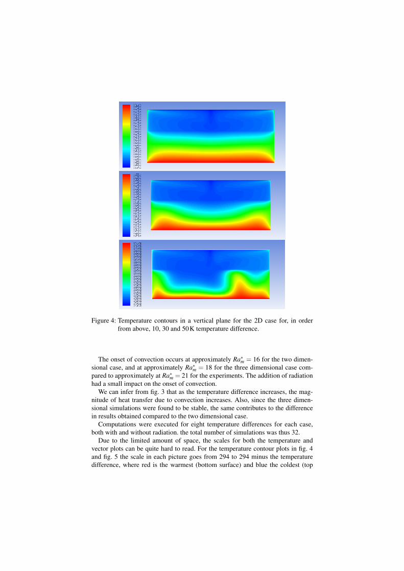
Figure 4: Temperature contours in a vertical plane for the 2D case for, in orderfrom above, 10, 30 and 50K temperature difference.

The onset of convection occurs at approximately Ra∗m = 16 for the two dimen-sional case, and at approximately Ra∗m = 18 for the three dimensional case com-pared to approximately at Ra∗m = 21 for the experiments. The addition of radiationhad a small impact on the onset of convection.

We can infer from fig. 3 that as the temperature difference increases, the mag-nitude of heat transfer due to convection increases. Also, since the three dimen-sional simulations were found to be stable, the same contributes to the differencein results obtained compared to the two dimensional case.

Computations were executed for eight temperature differences for each case,both with and without radiation. the total number of simulations was thus 32.

Due to the limited amount of space, the scales for both the temperature andvector plots can be quite hard to read. For the temperature contour plots in fig. 4and fig. 5 the scale in each picture goes from 294 to 294 minus the temperaturedifference, where red is the warmest (bottom surface) and blue the coldest (top

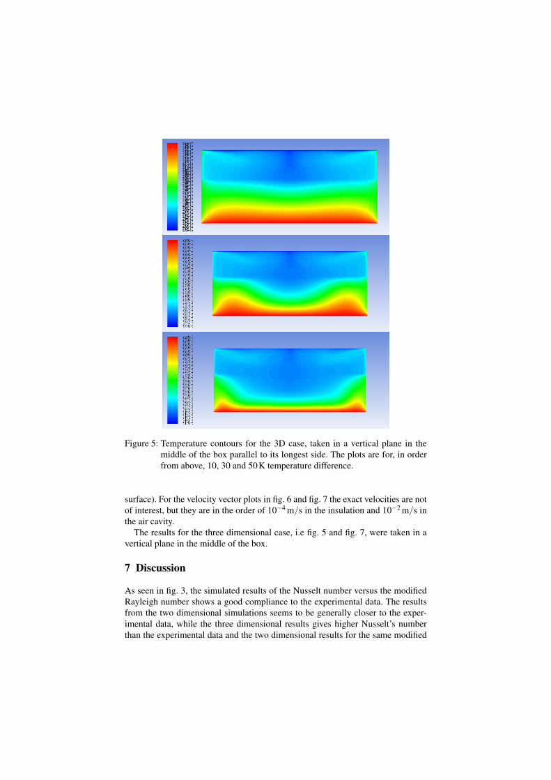
Figure 5: Temperature contours for the 3D case, taken in a vertical plane in themiddle of the box parallel to its longest side. The plots are for, in orderfrom above, 10, 30 and 50K temperature difference.

surface). For the velocity vector plots in fig. 6 and fig. 7 the exact velocities are notof interest, but they are in the order of 10−4 m/s in the insulation and 10−2 m/s inthe air cavity.

The results for the three dimensional case, i.e fig. 5 and fig. 7, were taken in avertical plane in the middle of the box.

7 Discussion

As seen in fig. 3, the simulated results of the Nusselt number versus the modifiedRayleigh number shows a good compliance to the experimental data. The resultsfrom the two dimensional simulations seems to be generally closer to the exper-imental data, while the three dimensional results gives higher Nusselt’s numberthan the experimental data and the two dimensional results for the same modified

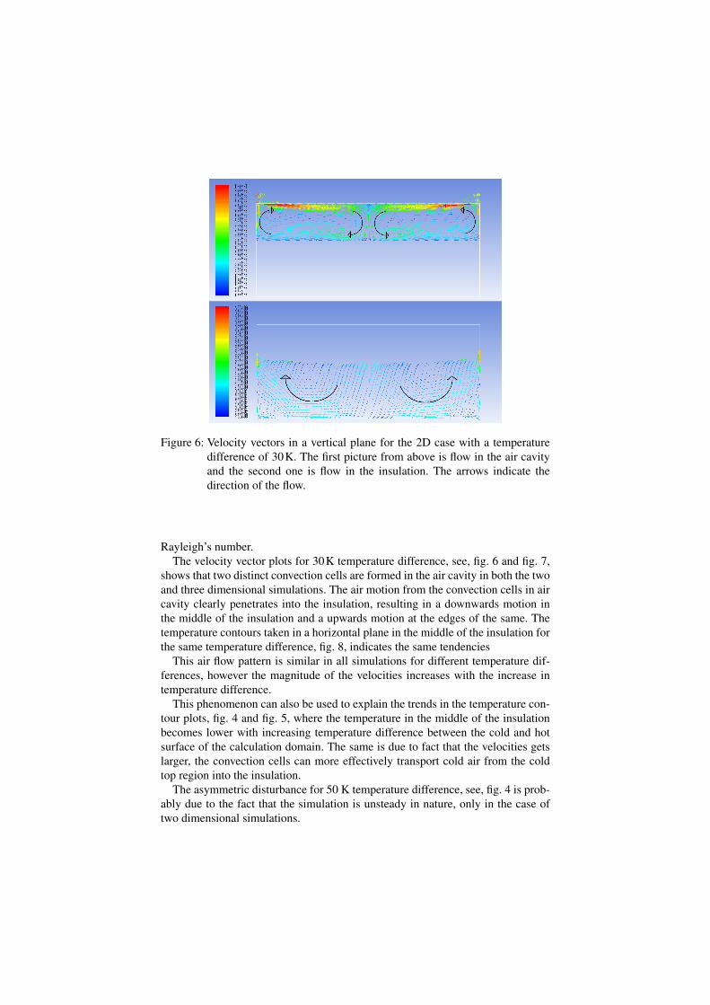
Figure 6: Velocity vectors in a vertical plane for the 2D case with a temperaturedifference of 30K. The first picture from above is flow in the air cavityand the second one is flow in the insulation. The arrows indicate thedirection of the flow.

Rayleigh’s number.The velocity vector plots for 30K temperature difference, see, fig. 6 and fig. 7,

shows that two distinct convection cells are formed in the air cavity in both the twoand three dimensional simulations. The air motion from the convection cells in aircavity clearly penetrates into the insulation, resulting in a downwards motion inthe middle of the insulation and a upwards motion at the edges of the same. Thetemperature contours taken in a horizontal plane in the middle of the insulation forthe same temperature difference, fig. 8, indicates the same tendencies

This air flow pattern is similar in all simulations for different temperature dif-ferences, however the magnitude of the velocities increases with the increase intemperature difference.

This phenomenon can also be used to explain the trends in the temperature con-tour plots, fig. 4 and fig. 5, where the temperature in the middle of the insulationbecomes lower with increasing temperature difference between the cold and hotsurface of the calculation domain. The same is due to fact that the velocities getslarger, the convection cells can more effectively transport cold air from the coldtop region into the insulation.

The asymmetric disturbance for 50 K temperature difference, see, fig. 4 is prob-ably due to the fact that the simulation is unsteady in nature, only in the case oftwo dimensional simulations.

Figure 7: Velocity vectors for the 3D case with a temperature difference of 30K,taken in a vertical plane in the middle of the box parallel to its longestside. The first picture from above is flow in the air cavity and the secondone is flow in the insulation. The arrows indicate the direction of theflow.

Figure 8: Temperature contours taken in a horizontal plane in the middle of theinsulation for the three dimensional case with a temperature differenceof 30K.

Regarding the accuracy of the numerical simulations, it can be seen when look-ing at the picture with the residuals, fig. 9, that they are in general low and stablefor both the two and three dimensional cases. The general convergence criterionin Fluent defines a converged solution when all residuals are below 10−3 exceptP1 and energy which have to be below 10−6 [13]. This criterion is sufficient inmost situations, and is fulfilled in both the two and three dimensional simulations.The highest residual is continuity in both cases but with a value between 10−2 to

Figure 9: Computational residuals for, in order from above, a two dimensional anda three dimensional case a the temperature difference of 30 K.

10−3 even this residual is quite low. This implies that the numerical error in thesimulations is low, and that the simulations should be of good quality.

As seen when comparing the simulations with and without radiation, the differ-ence is in general quite small, but the addition of radiation affects the convectiveheat flow more in the three dimensional case than in the two dimensional one.

8 Conclusion

The simulations show physical results both from a visual perspective (figures fortemperature and velocity distribution) and from a heat transfer perspective (fig. 3).The results obtained from computations are in agreement with the experiments.The applied method and model for porous media works well for this application.The magnitude of total rate of heat transfer is dependent on the temperature dif-ference across the domain. The heat transfer due to radiation also plays an impor-tant role. Three dimensional computations are recommended in order to obtain anaccurate picture of the flow field.

9 Future Work

Since the applied model for porous media works well for simulating the heat trans-fer in building insulation and also the buoyancy driven flow in the air cavity, more

complicated parts of buildings containing insulation, for example attics or walls ofbuildings, can now be numerically investigated using this model.

Acknowledgment

This research work has been conducted with the help of financial and computerresources obtained from AForsk, AF Industry AB, Sweden and the Division ofBuilding Technology, Chalmers University of Technology.

References

[1] Delmas, A. & Wilkes, K., Numerical analysis of heat transfer by conductionand natural convection in loose-fill fiber glass insulation effects of convec-tion on thermal insulation. ORNL/CON-338.

[2] Delmas, A. & Arquis, E., Early initiation of natural convection in an openedporous layer due to the presence of solid conductive inclusions. Journal ofHeat and Mass Transfer, 117.

[3] Shankar, V. & Hagentoft, C.E., Numerical convection in insulating porousmedium. Indoor air 99, Edinburgh.

[4] Shankar, V. & Hagentoft, C.E., Influence of natural convection on the ther-mal properties of insulating porous medium with air cavity. Indoor air 99,Edinburgh.

[5] Shankar, V. & Hagentoft, C.E., Numerical investigation of natural convec-tion in horizontal porous media heated from below comparisons with exper-iments. ASME International, Pittsburgh.

[6] Shankar, V., Davidson, L. & Olsson, E., Numerical investigation of turbulentplumes in both ambient and stratified surroundings. Journal of INDOOR AIR,Denmark.

[7] Shankar, V., Davidson, L. & Olsson, E., Ventilation by displacement: Calcu-lation of flow in vertical plumes. ROOM VENT, Aalborg, Denmark.

[8] Wahlgren, P., Convection in Loose-fill Attic Insulation. PhD Thesis, ChalmersUniversity of Technology, Goteborg, 2001.

[9] Serkitjis, M., Natural convection heat transfer in a horizontal thermal insu-lation layer underlying an air layer. PhD Thesis, Chalmers University ofTechnology, Goteborg, 1995.

[10] Andersson, B. & et al, Computational Fluid Dynamics for Engineers. Cam-bridge University Press: Cambridge, 2012.

[11] ANSYS, Inc, ANSYS FLUENT Theory Guide. ANSYS, Inc, Canonsburg, lat-est edition.

[12] Nield, D. & Bejan, A., Convection in Porous Media. Springer: New York,2013.

[13] ANSYS, Inc, ANSYS FLUENT User’s Guide. ANSYS, Inc, Canonsburg, lat-est edition.

Paper 2: Numerical Analysis of the Influence of

Natural Convection in Attics

Vijay Shankar, Head of Applied Research and Development at ÅF Industry AB. Andreas Bengtson and Victor Fransson, Masters in

Mechanical Engineering. Carl-Eric Hagentoft, Professor in Building Physics, Chalmers University of Technology.

Numerical Analysis of the Influence of Natural Convection in Attics - A CFD Analysis

Vijay Shankar Andreas Bengtson Victor Fransson

Carl-Eric Hagentoft

ABSTRACT HEADING

As the design of the building envelope has changed, the parameters that govern thermal insulation, air tightness and the complex hea t transfer

processes are often neglected. The aim of this research work is to numerically investigate the influence of natural convection in attics with joists and

insulation. With the help of Computational Fluid Dynamics (CFD), more specifically the software ANSYS Fluent, 3D simulations are

conducted for both porous layer and air cavity to estimate the magnitude of heat transfer. The same was executed for porous media for two different

values of permeability. A suitable turbulence model has been applied to account for the highly sensitive buoyancy driven flow. The results are

presented in form of dimensionless numbers, namely Nusselt number versus modified Rayleigh number. It can be concluded that the temperature

difference and permeability play a vital role on the influence of total heat transfer rate.

INTRODUCTION

The heat transfer processes are often the limiting factor when designing energy efficient buildings for sustainable

development. By investigating the heat flows and losses combined with the air movement in buildings, a greater

understanding and knowledge of the same can be obtained. Computational Fluid Dynamics (CFD) is a great tool in order

to examine these phenomena and to apply this knowledge in the process of designing energy efficient and sustainable

buildings.

When compared to real-life experiments, CFD simulations have several advantages. It is a more convenient and cost

effective method, since expensive experimental equipment is not needed.

In this research work, the heat transfer in a principal cold attic has been numerically investigated by using the

commercial CFD software ANSYS Fluent. The attic model consists of a horizontal layer of insulation with an overlying

region of air. The attic model can be viewed in cross section in Figure 1, along with its cross sectional dimensions. Besides

these dimensions, the attic is 1.8 m deep, the insulation has a maximum thickness of 0.4 m, and the angle of the roof is 20

degrees. At two sides of the insulation, wind deflectors are placed. They have the same angle as the roof, and are situated

there to prevent the ventilation system to force air to flow directly into the insulation. The presence of a ventilation system

is however not taken into account in this work.

Figure 1: The attic model, seen from the side. The upper region represents the air cavity and the lower one the porous insulation.

The model also includes the presence of wooden joists which are located within the insulation, see Figure 2. The joists are

assumed to have a significant impact on the overall heat transfer in the attic. The distance between the middle of two joists

is 0.6 m, and the joists have a width of 0.045 m and a height of 0.135 m. Each joist reaches from one side of the attic along

the floor to the other side.

The computational mesh for this research work consisted of 503390 cells and was constructed using only

hexahedronal cells in the software ANSYS ICEM.

Simulations were performed with a constant temperature at the bottom of the attic, Thot, of 294 K, and varying, lower,

temperatures at the boundary of the roof of the same, Tcold. The temperature difference was varied between 10 to 50 K.

Two different types of insulation with different values of permeability were investigated, in order to make a comparison and

analyze the impact of the permeability.

The applied virtual model for simulating the heat transfer in a medium containing both porous media as well as an air

cavity with help of CFD has been developed and verified by the authors in a previous work (Shankar et al., 2014)

This model is in turn based on previous research (Delmas, 1992), (Delmas, 1995), (Shankar, 1992), (Shankar, 1995),

(Shankar, 1999), (Shankar, 1999), (Shankar, 2000), (Wahlgren 2001) and verified by comparison to experimental work

performed by (Serkitjis, 1995).

NUMERICAL SETUP

The numerical setup for the simulations in this project was exactly the same as in the previous work in (Shankar et al.,

2014).

The applied boundary conditions for the attic were, with respect to the view in Figure 1, T=Tcold on the roof and the

sides that are in contact with the cold air, T=Thot on the bottom of the attic and q=0 on the vertical boundaries of the

insulation. In addition to this, symmetry boundary conditions were applied to the sides of the attic that are parallel to the

joists longitudinal direction. This was done in order to simulate that the attic continues in this direction rather than being

closed by walls.

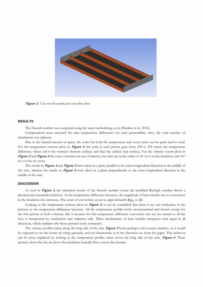
Figure 2: View over the wooden joists seen from above.

RESULTS

The Nusselt number was computed using the same methodology as in (Shankar et al., 2014).

Computations were executed for nine temperature differences for each permeability, thus, the total number of

simulations was eighteen.

Due to the limited amount of space, the scales for both the temperature and vector plots can be quite hard to read.

For the temperature contour plots in Figure 4, the scale in each picture goes from 294 to 294 minus the temperature

difference, where red is the warmest (bottom surface) and blue the coldest (top surface). For the velocity vector plots in

Figure 5 and Figure 6 the exact velocities are not of interest, but they are in the order of 10-4 m/s in the insulation and 10-2

m/s in the air cavity.

The results in Figure 4 and Figure 5 were taken in a plane parallel to the joists longitudinal direction in the middle of

the attic, whereas the results in Figure 6 were taken in a plane perpendicular to the joists longitudinal direction in the

middle of the attic.

DISCUSSION

As seen in Figure 3, the simulated results of the Nusselt number versus the modified Rayleigh number shows a

physical and reasonable behavior. As the temperature difference increases, the magnitude of heat transfer due to convection

in the insulation also increases. The onset of convection occurs at approximately .

Looking at the temperature contour plots in Figure 4, it can be concluded that there is no real tendencies in the

pictures as the temperature difference increases. All the temperature profiles looks unsymmetrical and chaotic except for

the first picture in both columns, this is because for this temperature difference convection has not yet started so all the

heat is transported by conduction and radiation only. These mechanisms of heat transfer transports heat equal in all

directions, which explains why those pictures looks symmetric.

The velocity profiles taken along the long side of the attic Figure 5 looks perhaps a bit counter intuitive, as it would

be expected to see the hotter air rising upwards, and not downwards or in the direction out from the paper. This behavior

can be more explained by looking at the temperature profiles taken across the long side of the attic, Figure 6. These

pictures show that the air above the insulation basically flows across the domain.

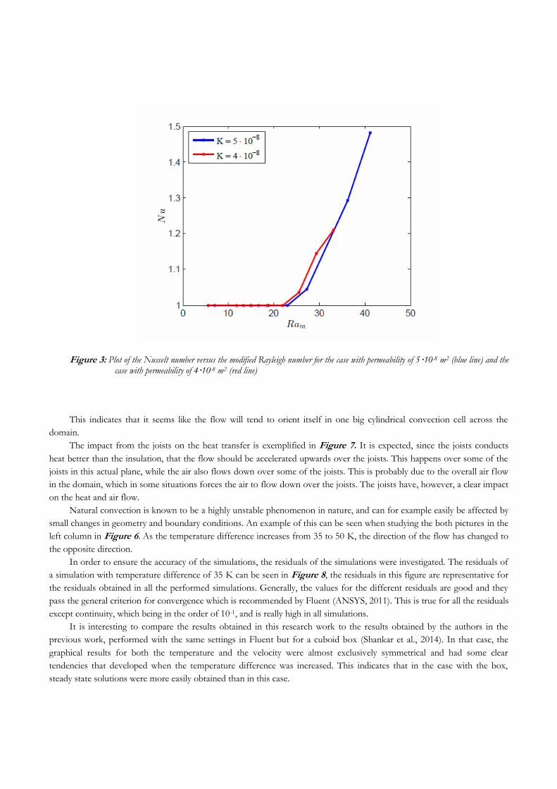
Figure 3: Plot of the Nusselt number versus the modified Rayleigh number for the case with permeability of 5·10-8 m2 (blue line) and the case with permeability of 4·10-8 m2 (red line)

This indicates that it seems like the flow will tend to orient itself in one big cylindrical convection cell across the

domain.

The impact from the joists on the heat transfer is exemplified in Figure 7. It is expected, since the joists conducts

heat better than the insulation, that the flow should be accelerated upwards over the joists. This happens over some of the

joists in this actual plane, while the air also flows down over some of the joists. This is probably due to the overall air flow

in the domain, which in some situations forces the air to flow down over the joists. The joists have, however, a clear impact

on the heat and air flow.

Natural convection is known to be a highly unstable phenomenon in nature, and can for example easily be affected by

small changes in geometry and boundary conditions. An example of this can be seen when studying the both pictures in the

left column in Figure 6. As the temperature difference increases from 35 to 50 K, the direction of the flow has changed to

the opposite direction.

In order to ensure the accuracy of the simulations, the residuals of the simulations were investigated. The residuals of

a simulation with temperature difference of 35 K can be seen in Figure 8, the residuals in this figure are representative for

the residuals obtained in all the performed simulations. Generally, the values for the different residuals are good and they

pass the general criterion for convergence which is recommended by Fluent (ANSYS, 2011). This is true for all the residuals

except continuity, which being in the order of 10-1, and is really high in all simulations.

It is interesting to compare the results obtained in this research work to the results obtained by the authors in the

previous work, performed with the same settings in Fluent but for a cuboid box (Shankar et al., 2014). In that case, the

graphical results for both the temperature and the velocity were almost exclusively symmetrical and had some clear

tendencies that developed when the temperature difference was increased. This indicates that in the case with the box,

steady state solutions were more easily obtained than in this case.

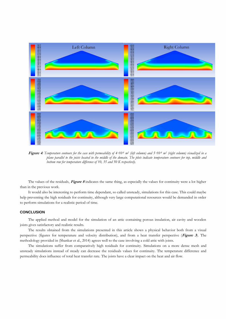
Figure 4: Temperature contours for the case with permeability of 4·10-8 m2 (left column) and 5·10-8 m2 (right column) visualized in a plane parallel to the joists located in the middle of the domain. The plots indicate temperature contours for top, middle and bottom row for temperature difference of 10, 35 and 50 K respectively.

The values of the residuals, Figure 8 indicates the same thing, as especially the values for continuity were a lot higher

than in the previous work.

It would also be interesting to perform time dependant, so called unsteady, simulations for this case. This could maybe

help preventing the high residuals for continuity, although very large computational resources would be demanded in order

to perform simulations for a realistic period of time.

CONCLUSION

The applied method and model for the simulation of an attic containing porous insulation, air cavity and wooden

joists gives satisfactory and realistic results.

The results obtained from the simulations presented in this article shows a physical behavior both from a visual

perspective (figures for temperature and velocity distribution), and from a heat transfer perspective (Figure 3). The

methodology provided in (Shankar et al., 2014) agrees well to the case involving a cold attic with joists.

The simulations suffer from comparatively high residuals for continuity. Simulations on a more dense mesh and

unsteady simulations instead of steady can decrease the residuals values for continuity. The temperature difference and

permeability does influence of total heat transfer rate. The joists have a clear impact on the heat and air flow.

Figure 5: Velocity vectors for the case with permeability of 4·10-8 m2 (left column) and 5·10-8 m2 (right column) visualized in a plane parallel to the joists located in the middle of the domain. The plots indicate velocity vectors for top and bottom row for temperature difference of 35 and 50 K respectively.

Figure 6: Velocity vectors for the case with permeability of 4·10-8 m2 (left column) and 5·10-8 m2 (right column) visualized in a plane perpendicular to the joists located in the middle of the domain. The plots indicate velocity vectors for top and bottom row for temperature difference of 35 and 50 K respectively.

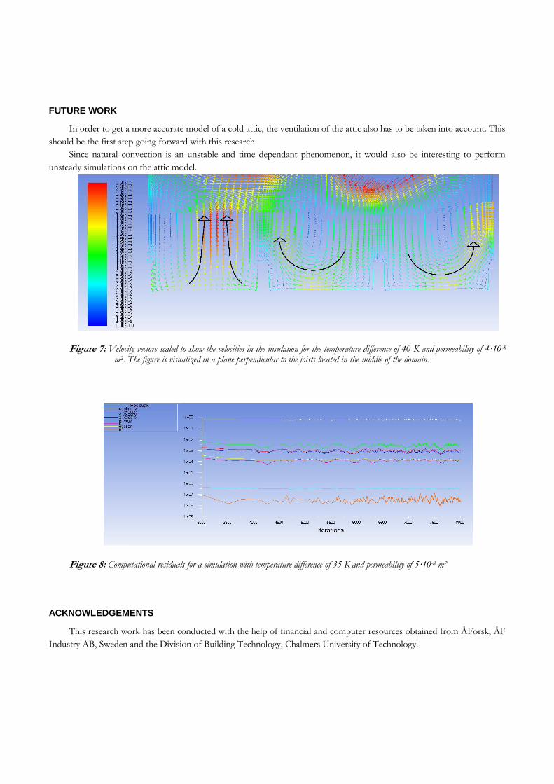
FUTURE WORK

In order to get a more accurate model of a cold attic, the ventilation of the attic also has to be taken into account. This

should be the first step going forward with this research.

Since natural convection is an unstable and time dependant phenomenon, it would also be interesting to perform

unsteady simulations on the attic model.

Figure 7: Velocity vectors scaled to show the velocities in the insulation for the temperature difference of 40 K and permeability of 4·10-8 m2. The figure is visualized in a plane perpendicular to the joists located in the middle of the domain.

Figure 8: Computational residuals for a simulation with temperature difference of 35 K and permeability of 5·10-8 m2

ACKNOWLEDGEMENTS

This research work has been conducted with the help of financial and computer resources obtained from ÅForsk, ÅF

Industry AB, Sweden and the Division of Building Technology, Chalmers University of Technology.

NOMENCLATURE

K = Permeability (m2)

Nu = Nusselt number

Ram = Modified Rayleigh number

= Critical modified Rayleigh number

= Temperature (K)

v = Velocity (m/s)

q = Heat Flux (W/m2)

= Porosity

Subscripts

m = material

REFERENCES

Andersson, B. et al. 2012. Computational Fluid Dynamics for Engineers. Cambridge University Press: Cambridge. ANSYS, Inc. 2011. ANSYS FLUENT Theory Guide. ANSYS, Inc, Canonsburg, latest edition. ANSYS, Inc. 2011. ANSYS FLUENT User’s Guide. ANSYS, Inc, Canonsburg, latest edition. Delmas, A. & Wilkes, K. 1992. Numerical analysis of heat transfer by conduction and natural convection in loose-fill fiber

glass insulation effects of convection on thermal insulation. ORNL/CON-338. Delmas, A. & Arquis, E.. 1995. Early initiation of natural convection in an opened porous layer due to the presence of solid

conductive inclusions. Journal of Heat and Mass Transfer, 117. Nield, D. & Bejan, A. 2013. Convection in Porous Media. Springer: New York. Serkitjis, M. 1995. Natural convection heat transfer in a horizontal thermal insulation layer underlying an air layer. PhD

Thesis, Chalmers University of Technology, Göteborg. Shankar, V., Bengtson, A., Fransson, V. & Hagentoft, C.E. 2014. Influence of Heat Transfer Processes in Porous Media

with Air Cavity - A CFD Analysis, Accepted for publication in the 8th International Conference on Computational and Experimental Methods in Multiphase and Complex Flow, Valencia, Spain, 20 - 22 April, 2015.

Shankar, V. & Hagentoft, C.E. 1999. Numerical convection in insulating porous medium. Indoor air 99, Edinburgh. Shankar, V. & Hagentoft, C.E. 1999. Influence of natural convection on the thermal properties of insulating porous

medium with air cavity. Indoor air 99, Edinburgh. Shankar, V. & Hagentoft, C.E. 2000. Numerical investigation of natural convection in horizontal porous media heated from

below comparisons with experiments. ASME International, Pittsburgh. Shankar, V., Davidson, L. & Olsson, E. 1995. Numerical investigation of turbulent plumes in both ambient and stratified

surroundings. Journal of INDOOR AIR, Denmark. Shankar, V., Davidson, L. & Olsson, E. 1992. Ventilation by displacement: Calculation of flow in vertical plumes. ROOM

VENT, Aalborg, Denmark. Wahlgren, P. 2001. Convection in Loose-fill Attic Insulation. PhD Thesis, Chalmers University of Technology, Göteborg.

Paper 3: CFD Analysis of Heat Transfer in Ven-

tilated Attics

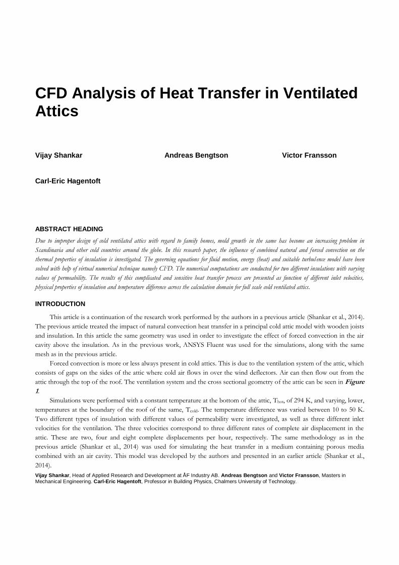
Vijay Shankar, Head of Applied Research and Development at ÅF Industry AB. Andreas Bengtson and Victor Fransson, Masters in

Mechanical Engineering. Carl-Eric Hagentoft, Professor in Building Physics, Chalmers University of Technology.

CFD Analysis of Heat Transfer in Ventilated Attics

Vijay Shankar Andreas Bengtson Victor Fransson

Carl-Eric Hagentoft

ABSTRACT HEADING

Due to improper design of cold ventilated attics with regard to family homes, mold growth in the same has become an increasing problem in

Scandinavia and other cold countries around the globe. In this research paper, the influence of combined natural and forced convection on the

thermal properties of insulation is investigated. The governing equations for fluid motion, energy (heat) and suitable turbul ence model have been

solved with help of virtual numerical technique namely CFD. The numerical computations are conducted for two different insulations with varying

values of permeability. The results of this complicated and sensitive heat transfer process are presented as function of different inlet velocities,

physical properties of insulation and temperature difference across the calculation domain for full scale cold ventilated attics.

INTRODUCTION

This article is a continuation of the research work performed by the authors in a previous article (Shankar et al., 2014).

The previous article treated the impact of natural convection heat transfer in a principal cold attic model with wooden joists

and insulation. In this article the same geometry was used in order to investigate the effect of forced convection in the air

cavity above the insulation. As in the previous work, ANSYS Fluent was used for the simulations, along with the same

mesh as in the previous article.

Forced convection is more or less always present in cold attics. This is due to the ventilation system of the attic, which

consists of gaps on the sides of the attic where cold air flows in over the wind deflectors. Air can then flow out from the

attic through the top of the roof. The ventilation system and the cross sectional geometry of the attic can be seen in Figure

1.

Simulations were performed with a constant temperature at the bottom of the attic, Thot, of 294 K, and varying, lower,

temperatures at the boundary of the roof of the same, Tcold. The temperature difference was varied between 10 to 50 K.

Two different types of insulation with different values of permeability were investigated, as well as three different inlet

velocities for the ventilation. The three velocities correspond to three different rates of complete air displacement in the

attic. These are two, four and eight complete displacements per hour, respectively. The same methodology as in the

previous article (Shankar et al., 2014) was used for simulating the heat transfer in a medium containing porous media

combined with an air cavity. This model was developed by the authors and presented in an earlier article (Shankar et al.,

2014).

Figure 1: The attic model, seen from the side. The upper region represents the air cavity and the lower one the porous insulation. The upper picture shows the dimensions of the principle attic model, and the lower picture visually represents the inlet and outlet of the ventilation system.

This model is in turn based on previous research (Delmas, 1992), (Delmas, 1995), (Shankar, 1992), (Shankar, 1995),

(Shankar, 1999), (Shankar, 1999), (Shankar, 2000), (Wahlgren 2001) and verified by comparison to experimental work

performed by (Serkitjis, 1995).

NUMERICAL SETUP

The same numerical setup as in the previous work (Shankar et al., 2014a), (Shankar et al., 2014b). was used for the

simulations presented in this article.

The boundary conditions applied for the attic model were mostly identical to the boundary conditions used in the

investigation of natural convection in the attic (Shankar et al., 2014). These include specified constant temperatures of

T=Tcold on the roof of the attic, and T=Thot on the floor of the attic. The vertical boundaries in contact with the insulation

were set to have a heat flux of q=0, and a symmetry boundary condition were specified for the sides of the attic parallel to

the joists longitudinal direction.

The differences in boundary conditions between the case with only natural convection (Shankar et al., 2014) and the

cases including forced convection was the modeling of the ventilation system. The boundaries situated between the wind

deflectors and the roof were set to velocity inlets, with the inlet velocity set to correspond to the particular rate of complete

air displacement of the simulation. The temperature of the inlet air was set to T=Tcold. A pressure outlet boundary

condition with atmospheric pressure was specified for the boundary at the very top of the roof. In Figure 1, the exact

position of these boundaries can be seen.

Figure 2: Plot of the Nusselt number versus the modified Rayleigh number for the cases with permeability of 4·10-8 m2 (the three dashed lines) and the cases with permeability of 5·10-8 m2 (the three solid lines). L2, L4 and L8 represents two, four and eight complete air displacements per hour, respectively.

RESULTS

The Nusselt number was computed in the same way as (Shankar et al., 2014a) and (Shankar et al., 2014b).

For each rate of air exchange, nine temperature differences were computed. Since two different permeabilities were

investigated, the total number of simulations for this work was 54.

The scale in each temperature contour picture goes from 294 to 294 minus the temperature difference, with red being

the warmest temperatures (bottom surface) and blue being the coldest (top surface). The temperature contour plots can be

seen in Figure 4

The velocity vectors can be seen in Figure 5 and Figure 6. The exact velocities in these pictures are not of large

interest.

A plane parallel to the joists longitudinal direction in the middle of the attic was used to display the results in Figure 4

and Figure 5, whereas a plane perpendicular to the joists longitudinal direction in the middle of the attic was used to

display the results in Figure 6.

DISCUSSION

As can be seen in Figure 2, the different air displacement rates generally have a small effect on the Nusselt versus the

modified Rayleigh number curves. This means that the influence of the forced convective part on the total convection is

not that significant. The shapes of the curves are also very similar to those representing the case of pure natural convection

(Shankar et al., 2014). However, as the temperature difference increases across the calculation domain, the influence of

mixed convection also increases.

Figure 3: Plots of the Nusselt number versus the Reynolds number. The picture to the left is for the cases with permeability of 4·10-8 m2

and the picture to the right for 5·10-8 m2. The Reynolds number is based on the diameter of the inlet to the attic. Each line represents one temperature difference.

The onset of natural convection occurs, just like in the simulations involving pure natural convection, approximately

at . The different air displacement rate does not affect the onset of natural convection.

Although the curves look very similar in Figure 2, there are some distinctions which can be seen clearly when

analyzing the Nusselt number versus the Reynolds number in Figure 3. These pictures show that as the Reynolds number,

i.e. the inlet velocity, increases, the Nusselt number generally decreases. This means that the influence of the total

convection decreases with increasing velocity. Also, the magnitude of mixed convection increases with increasing

temperature difference.

Figure 4 shows how the temperature field changes as the ventilation rate goes from two to eight air displacements per

hour for the temperature differences of 35 and 50 K and the permeability of 4·10-8 m2. It is hard to see any tendencies in

these figures as the ventilation rate becomes higher, all the pictures looks very unsymmetrical. In the previous work with

only natural convection on the attic model, the temperature contour plots were also very unsymmetrical and irregular, and

showed no real trends as the temperature increased (Shankar et al., 2014). However, in the results from the simulations on

the box model, (Shankar et al., 2014), there were clear trends in the figures as the temperature increased. Also, essentially all

these simulations showed symmetrical results for the temperature contours. Based on this, it seems like the simulations for

the attic model, both with and without ventilation enabled, were a lot more unsteady than in the case of the box model.

The difference in the flow field due to the different air flow rates can be viewed for the temperature difference of 35

K in Figure 5 and Figure 6. These pictures show the difference in the flow field when the air displacement rates are two

respectively eight complete displacements per hour. The flow field pictures taken in a plane parallel to the joists, Figure 5,

shows that the same flow pattern occurs for both the permeabilities. The inlet air forces the air in the attic to flow towards

the middle of the air cavity of the attic and further out through the outlet on the top of the roof, with increased velocity

when the air displacement rate increases.

The flow field pictures taken in a plane perpendicular to the joists, Figure 6 shows some interesting phenomena. As

seen in the upper picture in both those figures, swirls have been developed in the air cavity for the lower air displacement

rate. When the ventilation rate increases to eight air displacements per hour both these swirls are gone.

Figure 4: Example of temperature contours for simulations with permeability of 4·10-8 m2 and varying rate of ventilation. The column to the left represents simulations with temperature difference of 35 K and the column to the right represents a temperature difference 50 K. The first picture (row 1) from above represents a ventilation rate of two complete air displacements per hour and the second (row 2) represents eight. The plots are visualized in a plane parallel to the joists located in the middle of the domain.

This is probably due to as the ventilation rate increases, the overall flow field in the attic becomes more structured

which prevents the formation of swirls and other irregular flow phenomena.

The accuracy of the simulations has been verified in two ways. Firstly, the mass flow in and out has been compared.

These results showed that the net mass flow for all of the performed simulations was very close to zero, which implies that

continuity is ensured. Secondly, the computational residuals of the simulations have been investigated. For the simulation

case with a temperature difference of 35 K, a complete air displacement rate of two times per hour, and permeability of

5·10-8 m2 the residuals are presented in Figure 7. These residuals are representable for how the residuals looked like for the

simulations in this research work. The figure shows that the residuals are relatively low in general and does not, except for

the radiation equation residuals (P1), fluctuate very much. However, just as in the previous work with only natural

convection on the attic model (Shankar et al., 2014) the residuals for continuity are, with a value around 4·10-1, really high.

The values for all other residuals are good and all of them pass the general convergence criterion by Fluent (ANSYS, 2011).

CONCLUSION

As in the work conducted by the authors (Shankar et al., 2014a), (Shankar et al., 2014b) the results when applying this

methodology of simulating heat transfer and fluid flow in a porous media combined with an air cavity show a physically

reasonable behavior. With the addition of a ventilation system, the applied attic model has become even more realistic and

physical.

The accuracy of the simulations has been verified by studying the net mass flux into the domain, and also by

examining the computational residuals for the simulations. Except from high residuals in continuity, the simulations seem

accurate in a numerical way.

The results of the simulations involving forced convection show that the heat transfer in the insulation is largely

unaffected by the addition of a ventilation system for this specific attic geometry. The inlet flow mainly affects the fluid

movements in the air cavity.

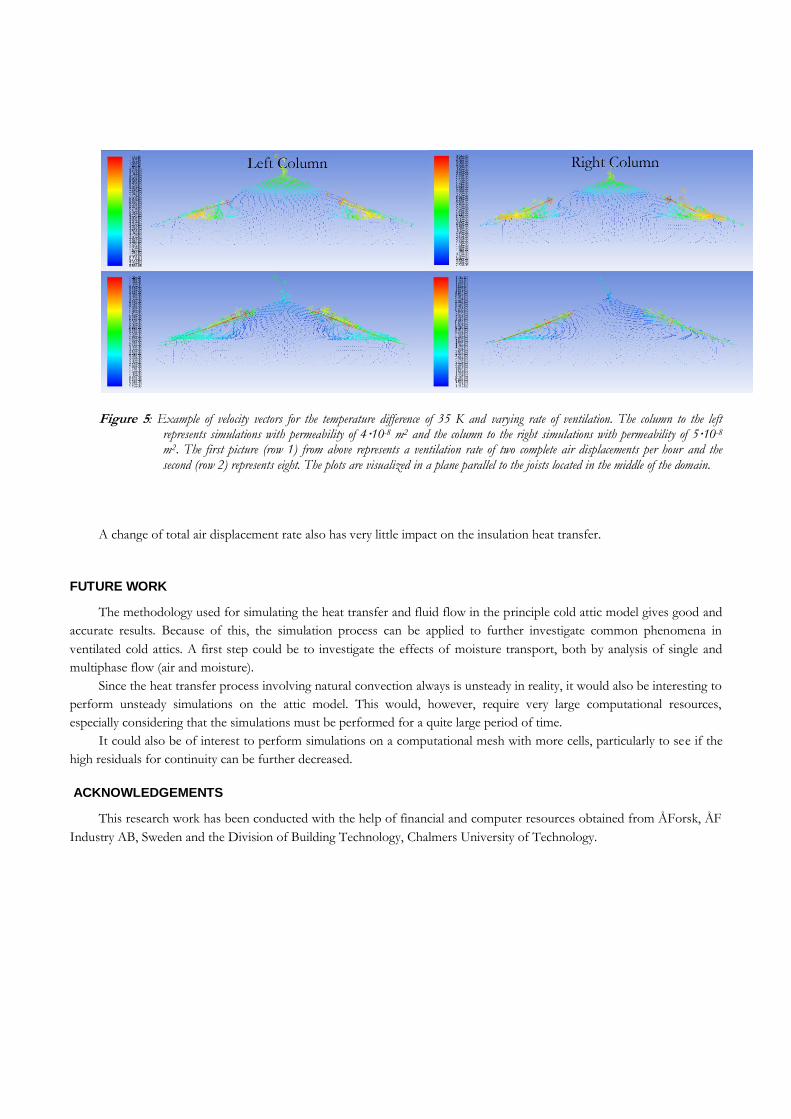
Figure 5: Example of velocity vectors for the temperature difference of 35 K and varying rate of ventilation. The column to the left represents simulations with permeability of 4·10-8 m2 and the column to the right simulations with permeability of 5·10-8 m2. The first picture (row 1) from above represents a ventilation rate of two complete air displacements per hour and the second (row 2) represents eight. The plots are visualized in a plane parallel to the joists located in the middle of the domain.

A change of total air displacement rate also has very little impact on the insulation heat transfer.

FUTURE WORK

The methodology used for simulating the heat transfer and fluid flow in the principle cold attic model gives good and

accurate results. Because of this, the simulation process can be applied to further investigate common phenomena in

ventilated cold attics. A first step could be to investigate the effects of moisture transport, both by analysis of single and

multiphase flow (air and moisture).

Since the heat transfer process involving natural convection always is unsteady in reality, it would also be interesting to

perform unsteady simulations on the attic model. This would, however, require very large computational resources,

especially considering that the simulations must be performed for a quite large period of time.

It could also be of interest to perform simulations on a computational mesh with more cells, particularly to see if the

high residuals for continuity can be further decreased.

ACKNOWLEDGEMENTS

This research work has been conducted with the help of financial and computer resources obtained from ÅForsk, ÅF

Industry AB, Sweden and the Division of Building Technology, Chalmers University of Technology.

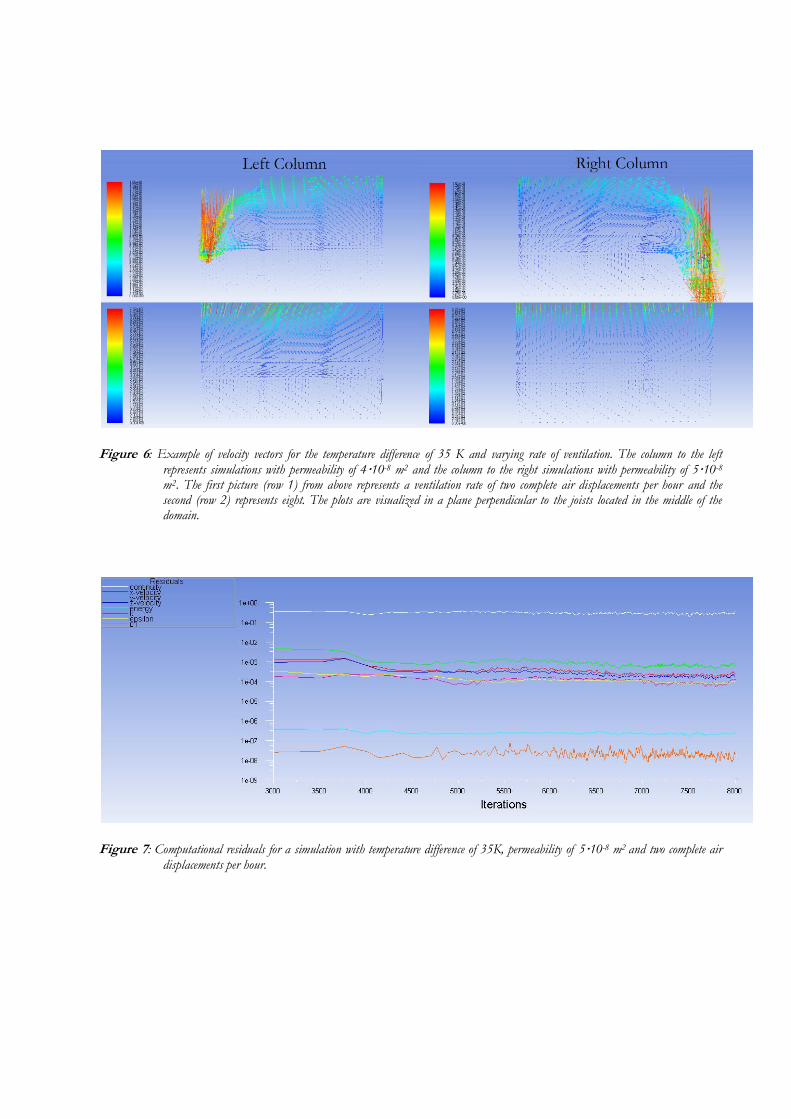
Figure 6: Example of velocity vectors for the temperature difference of 35 K and varying rate of ventilation. The column to the left represents simulations with permeability of 4·10-8 m2 and the column to the right simulations with permeability of 5·10-8 m2. The first picture (row 1) from above represents a ventilation rate of two complete air displacements per hour and the second (row 2) represents eight. The plots are visualized in a plane perpendicular to the joists located in the middle of the domain.

Figure 7: Computational residuals for a simulation with temperature difference of 35K, permeability of 5·10-8 m2 and two complete air displacements per hour.

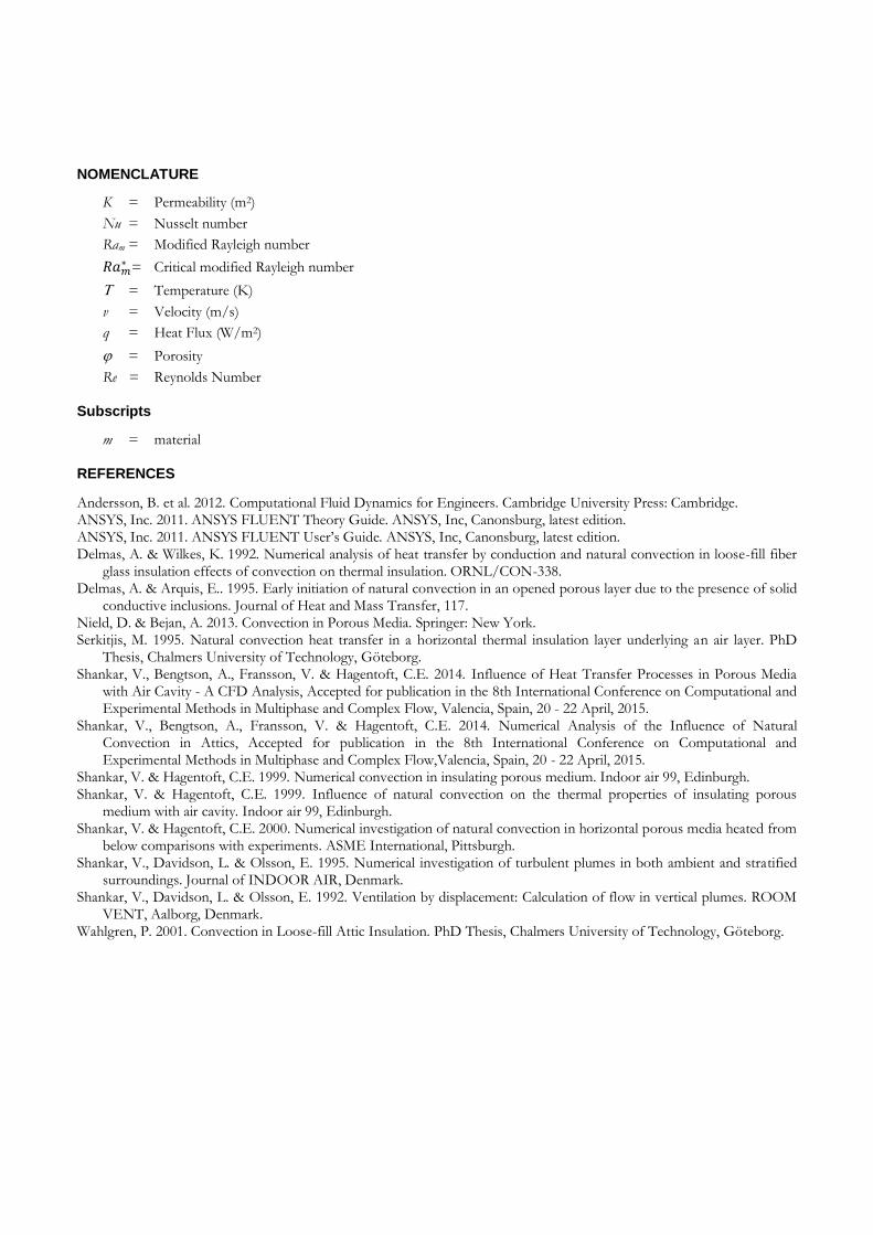
NOMENCLATURE

K = Permeability (m2)

Nu = Nusselt number

Ram = Modified Rayleigh number

= Critical modified Rayleigh number

= Temperature (K)

v = Velocity (m/s)

q = Heat Flux (W/m2)

= Porosity

Re = Reynolds Number

Subscripts

m = material

REFERENCES

Andersson, B. et al. 2012. Computational Fluid Dynamics for Engineers. Cambridge University Press: Cambridge. ANSYS, Inc. 2011. ANSYS FLUENT Theory Guide. ANSYS, Inc, Canonsburg, latest edition. ANSYS, Inc. 2011. ANSYS FLUENT User’s Guide. ANSYS, Inc, Canonsburg, latest edition. Delmas, A. & Wilkes, K. 1992. Numerical analysis of heat transfer by conduction and natural convection in loose-fill fiber

glass insulation effects of convection on thermal insulation. ORNL/CON-338. Delmas, A. & Arquis, E.. 1995. Early initiation of natural convection in an opened porous layer due to the presence of solid

conductive inclusions. Journal of Heat and Mass Transfer, 117. Nield, D. & Bejan, A. 2013. Convection in Porous Media. Springer: New York. Serkitjis, M. 1995. Natural convection heat transfer in a horizontal thermal insulation layer underlying an air layer. PhD

Thesis, Chalmers University of Technology, Göteborg. Shankar, V., Bengtson, A., Fransson, V. & Hagentoft, C.E. 2014. Influence of Heat Transfer Processes in Porous Media

with Air Cavity - A CFD Analysis, Accepted for publication in the 8th International Conference on Computational and Experimental Methods in Multiphase and Complex Flow, Valencia, Spain, 20 - 22 April, 2015.

Shankar, V., Bengtson, A., Fransson, V. & Hagentoft, C.E. 2014. Numerical Analysis of the Influence of Natural Convection in Attics, Accepted for publication in the 8th International Conference on Computational and Experimental Methods in Multiphase and Complex Flow,Valencia, Spain, 20 - 22 April, 2015.

Shankar, V. & Hagentoft, C.E. 1999. Numerical convection in insulating porous medium. Indoor air 99, Edinburgh. Shankar, V. & Hagentoft, C.E. 1999. Influence of natural convection on the thermal properties of insulating porous

medium with air cavity. Indoor air 99, Edinburgh. Shankar, V. & Hagentoft, C.E. 2000. Numerical investigation of natural convection in horizontal porous media heated from

below comparisons with experiments. ASME International, Pittsburgh. Shankar, V., Davidson, L. & Olsson, E. 1995. Numerical investigation of turbulent plumes in both ambient and stratified

surroundings. Journal of INDOOR AIR, Denmark. Shankar, V., Davidson, L. & Olsson, E. 1992. Ventilation by displacement: Calculation of flow in vertical plumes. ROOM

VENT, Aalborg, Denmark. Wahlgren, P. 2001. Convection in Loose-fill Attic Insulation. PhD Thesis, Chalmers University of Technology, Göteborg.