Embed Size (px)
Citation preview
PartitioningPartitioning• “He who can properly define and
divide is to be considered a god.”Plato (ca 429-347 BC)

System PartitioningSystem Partitioning1. The functionality of a system is implemented with a set
of interconnected system components, such as ASIC’s, memories, CPU’s, buses.
2. The designer must solve two problemstwo problems:• select a set of system components (allocation),• partition the system’s functionality among these components
(partitioning).
3. The final implementation has to satisfy a set of design constraints, such as:• cost, cost, • performance andperformance and• power consumptionpower consumption
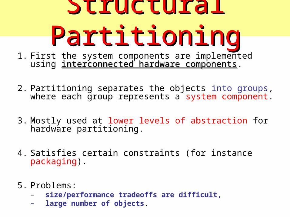
Structural PartitioningStructural Partitioning1. First the system components are implemented using
interconnected hardware componentsinterconnected hardware components.
2. Partitioning separates the objects into groups, where each group represents a system component.
3. Mostly used at lower levels of abstraction for hardware partitioning.
4. Satisfies certain constraints (for instance packaging).
5. Problems:– size/performance tradeoffs are difficult,– large number of objects.
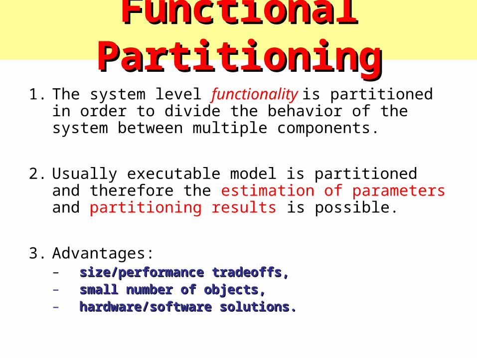
Functional PartitioningFunctional Partitioning1. The system level functionality is partitioned in order to
divide the behavior of the system between multiple components.
2. Usually executable model is partitioned and therefore the estimation of parameters and partitioning results is possible.
3. Advantages:– size/performance tradeoffs,size/performance tradeoffs,– small number of objects,small number of objects,– hardware/software solutions.hardware/software solutions.

Partitioning GranularityPartitioning Granularity
1.1. Coarse granularityCoarse granularity• deals with
• processes, • subprograms, • blocks of statements,
• typical for system-level synthesis,• deals with a relatively small number of objects.
2. Fine granularityFine granularity• performed at operation level,• used during high-level synthesis,• high complexity.
Abstract RepresentationAbstract Representation
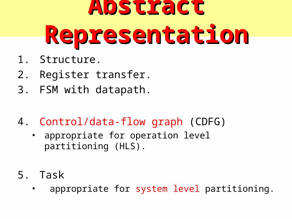
1. Structure.
2. Register transfer.
3. FSM with datapath.
4. Control/data-flow graph (CDFG)• appropriate for operation level partitioning (HLS).
5. Task• appropriate for system level partitioning.
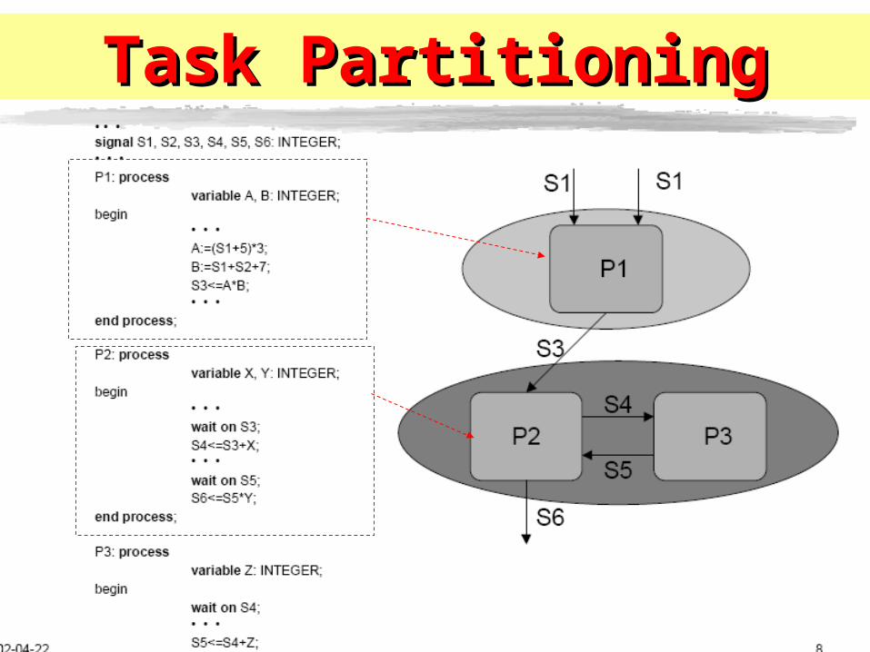
Task PartitioningTask Partitioning
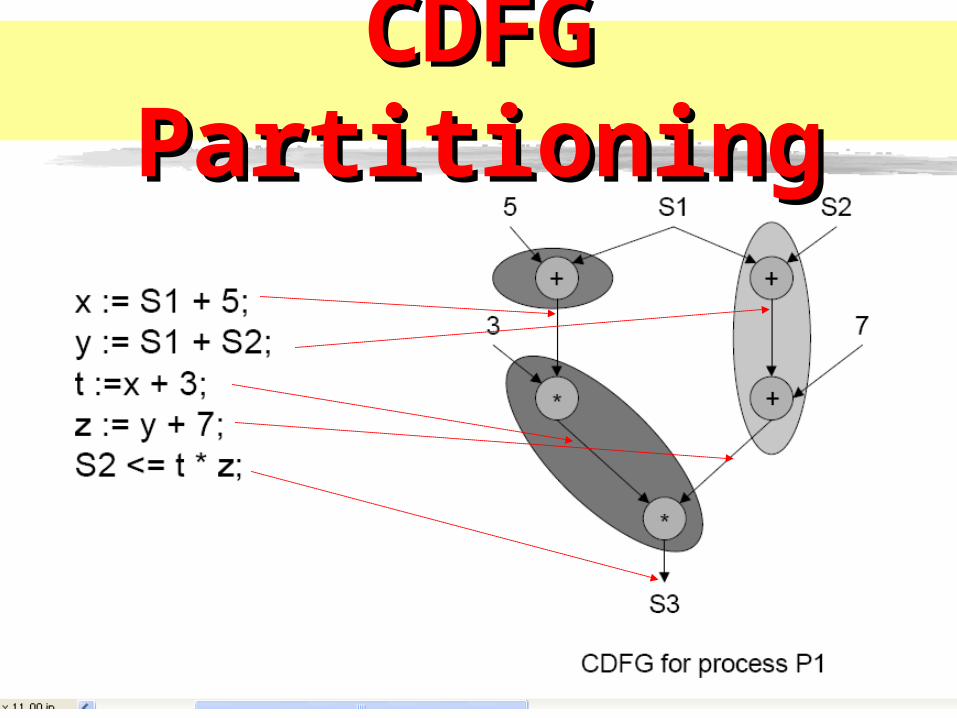
CDFG PartitioningCDFG Partitioning

System PartitioningSystem Partitioning
Metrics and EstimationsMetrics and Estimations
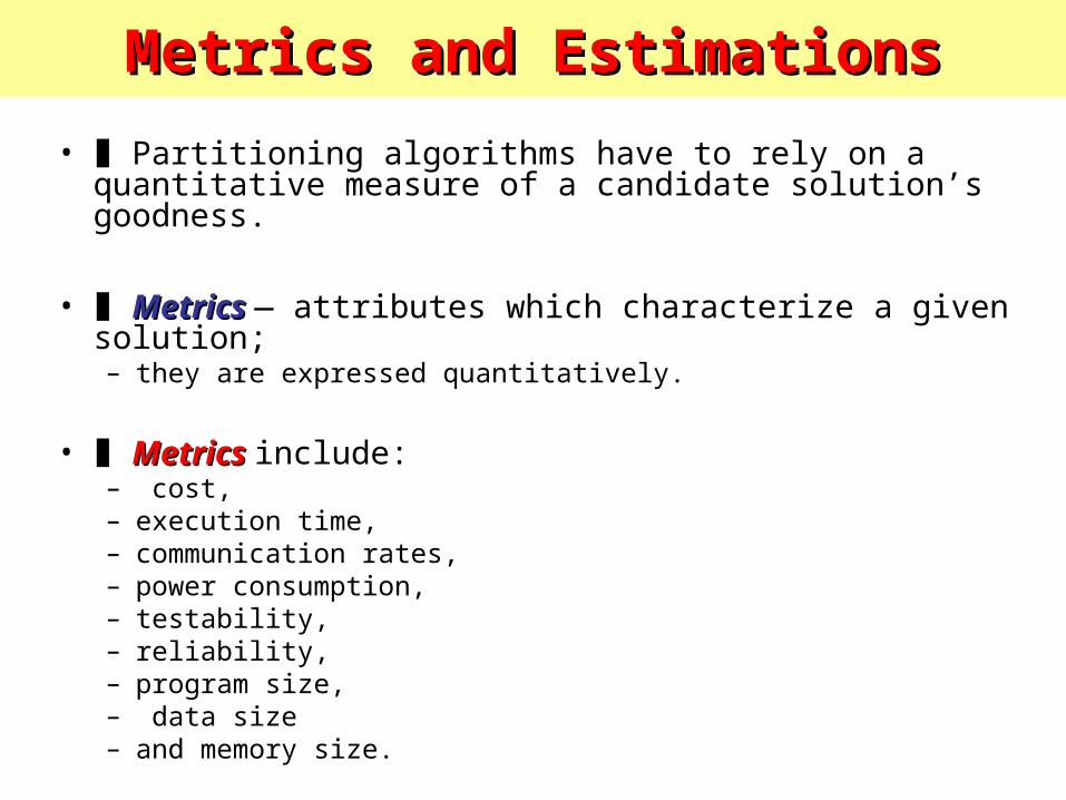
• ❚ Partitioning algorithms have to rely on a quantitative measure of a candidate solution’s goodness.
• ❚ MetricsMetrics — attributes which characterize a given solution;– they are expressed quantitatively.
• ❚ MetricsMetrics include:– cost, – execution time, – communication rates, – power consumption, – testability,– reliability, – program size,– data size – and memory size.
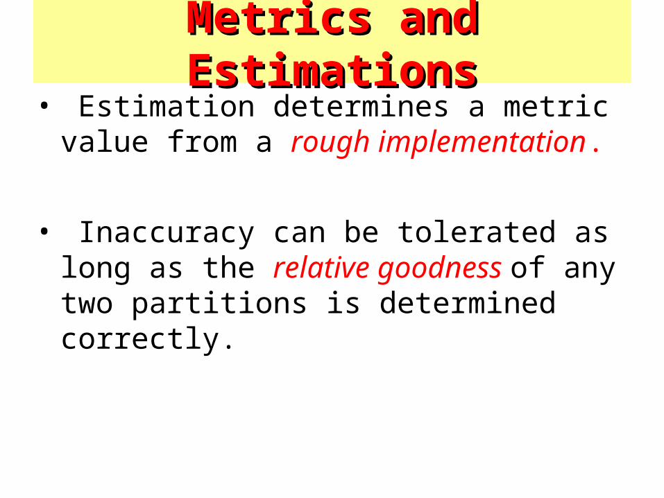
Metrics and EstimationsMetrics and Estimations• Estimation determines a metric value from
a rough implementation.
• Inaccuracy can be tolerated as long as the relative goodness of any two partitions is determined correctly.

Objective Function and Objective Function and Closeness functionCloseness function
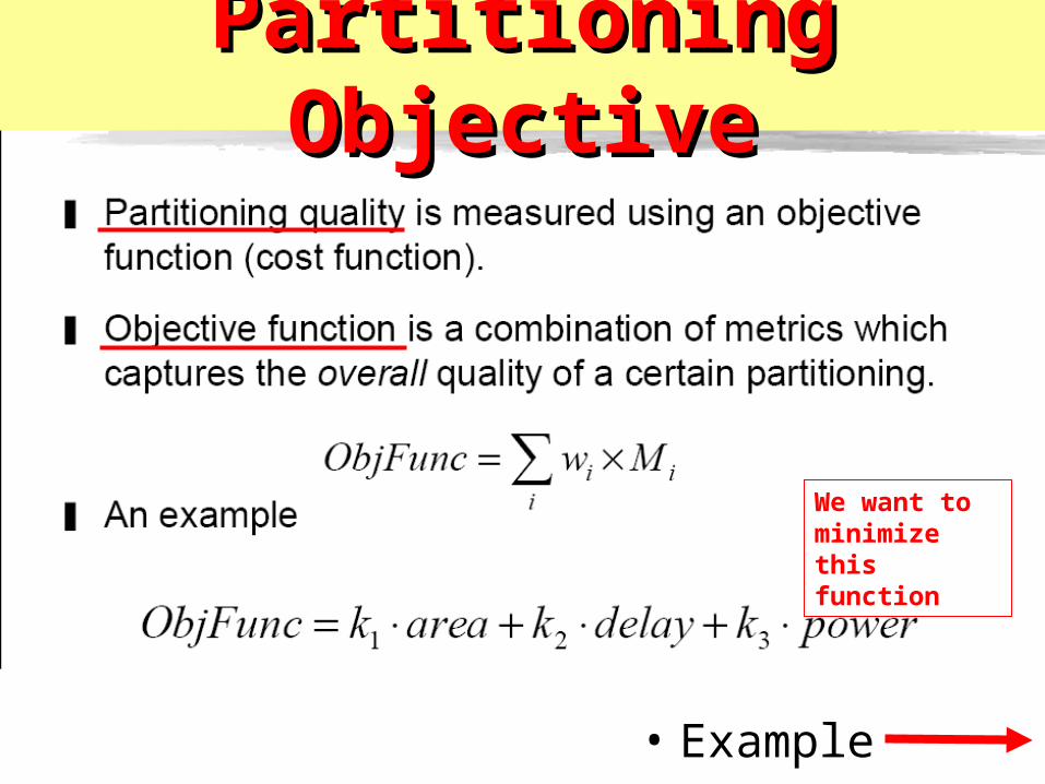
1. Objective functionObjective function: • a combination of metrics which captures the
overall overall qualityquality of a certain partitioning.
2. Closeness functionCloseness function: • captures the benefit gained from grouping
two objects into the same partition;• it is based on a local local viewview of the system.
• Example
Partitioning ObjectivePartitioning Objective
We want to minimize this function
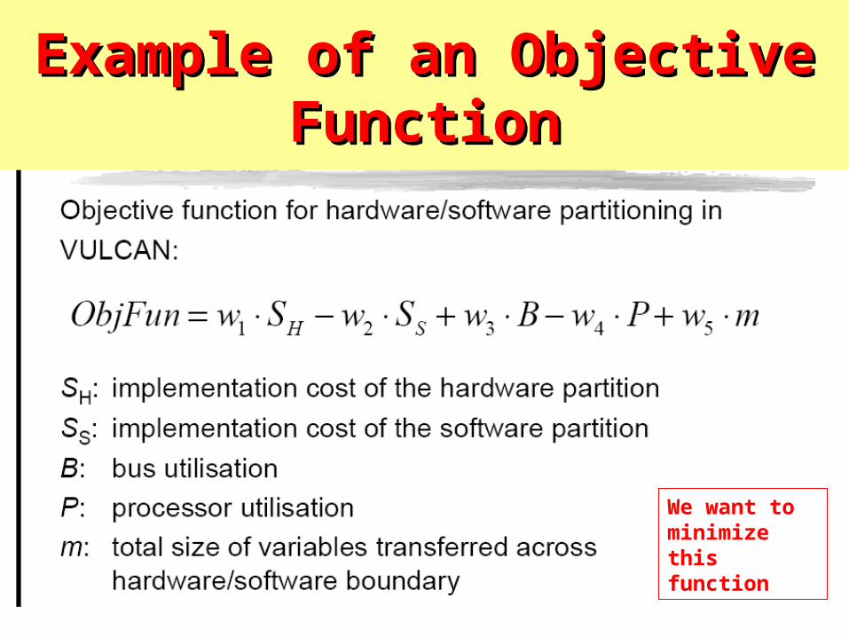
Example of an Objective Example of an Objective FunctionFunction
We want to minimize this function

Design ConstraintsDesign Constraints
We want to minimize this function

Example of an Objective Example of an Objective FunctionFunction
We want to minimize this function
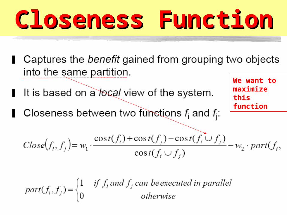
Closeness FunctionCloseness Function
We want to maximize this function
Partitioning ApproachesPartitioning Approaches
1. Manually guided partitioning
2. Needs strong support from design environment:– estimation tools & schedulers,– facilities to interactively perform predefined
transformations and to define new ones,– graphical interfaces.
3. Automatic partitioning
Automatic PartitioningAutomatic Partitioning
1. The partitioning problem is is NP-NP-complete.complete.
2. The design space has to be explored according to a certain strategy
3. This strategy converges towards a solution close to one which yields the minimal cost.
Automatic Partitioning Automatic Partitioning ApproachesApproaches
• ConstructiveConstructive (clustering)
– bottom up approach: • each object initially belongs to its own cluster, • and clusters are then gradually merged until the
desired partitioning is found;
– does not require a global view of the system– relies only on local relations between objects
(closeness metrics).
Automatic Partitioning Automatic Partitioning Approaches (cont’d)Approaches (cont’d)
• IterativeIterative (transformation-based)– based on a design space exploration which is
guided by an objective functionobjective function that reflects the global quality of the partitioning;
• a starting solution is modified iteratively,
• by passing from one candidate solution to another
• passing is based on evaluations of an objective function.
Hierarchical clusteringHierarchical clustering
• A constructive approach:A constructive approach: – performed in several iterations – with final goal to group a set of objects into partitions
according to some measure of closeness.
• At each iteration the two closest objectstwo closest objects are grouped together; – the process is iterated until a single cluster is
produced.

Hierarchical cluster treeHierarchical cluster tree1. The cluster tree contains
• leafsleafs:: original objects• internal nodesinternal nodes:: clustered objects• heightheight:: associated to each non-terminal node;
• reflects the distance between the two objects that have been merged into the corresponding cluster.
2. A certain partitioning is selected by cutting the cluster tree with a “cut line”; • each subtree below the cut line becomes one resulting partition.
3. The closeness function is defined between the initial objects; • at successive iterations, closeness between different groups of
objects have to be estimated estimated based on the closeness between individual objects.
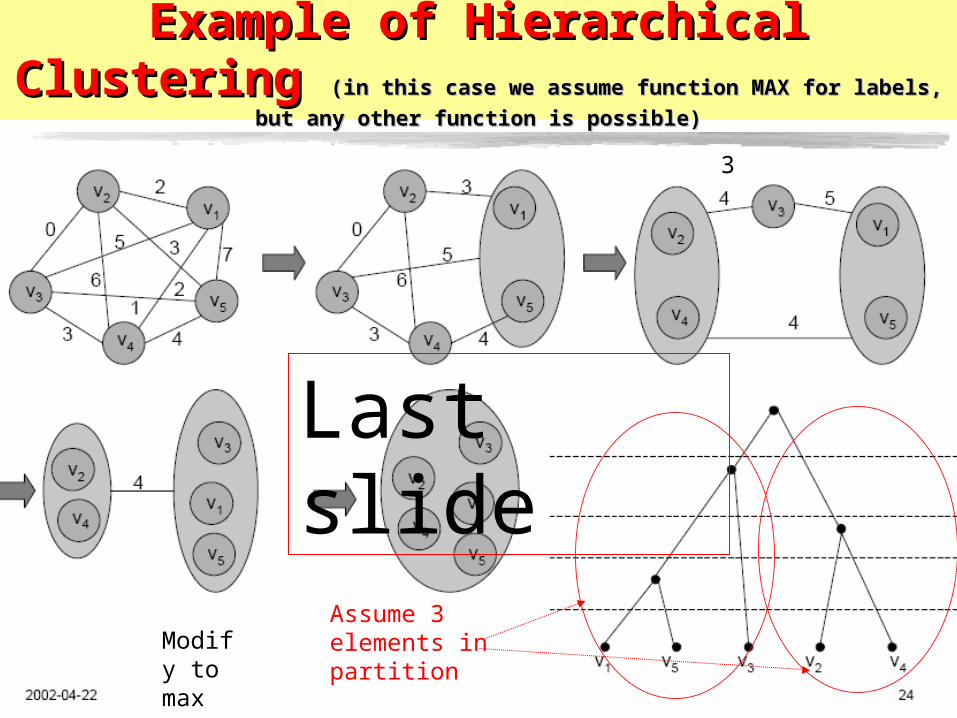
Example of Hierarchical Clustering Example of Hierarchical Clustering (in this case (in this case
we assume function MAX for labels, but any other function is possible)we assume function MAX for labels, but any other function is possible)
Modify to max
Assume 3 elements in partition
Last slide
3
Transformation Based Transformation Based PartitioningPartitioning
• Transformation based approaches perform different variants of neighborhood searchneighborhood search..
• Neighborhood N(x) of a solution x is a set of solutions that can be reached from x by a simple operation (move).
• Greedy partitioning algorithms have tendency to be trapped in local minima.
• There exist algorithms which help to escape from local minima:– Kernighan-Lin, – Simulated Annealing, – Tabu Search, – Genetic Algorithms,– etc.
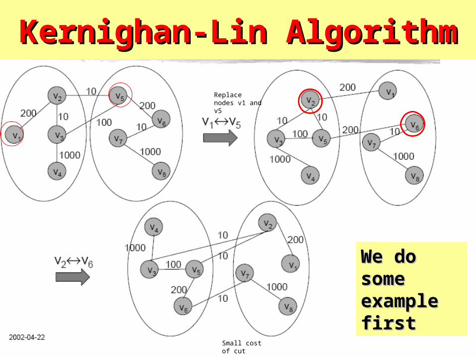
Kernighan-Lin AlgorithmKernighan-Lin Algorithm
Replace nodes v1 and v5
Small cost of cut
We do We do some some example example firstfirst

Kerninghan-Lin algorithmKerninghan-Lin algorithm
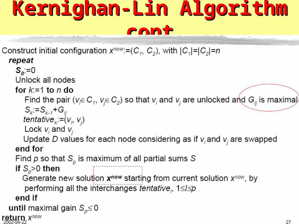
Kernighan-Lin Algorithm contKernighan-Lin Algorithm cont

Objective Function in Kernighan-Lin Objective Function in Kernighan-Lin AlgorithmAlgorithm
KL and similar algorithmsKL and similar algorithms
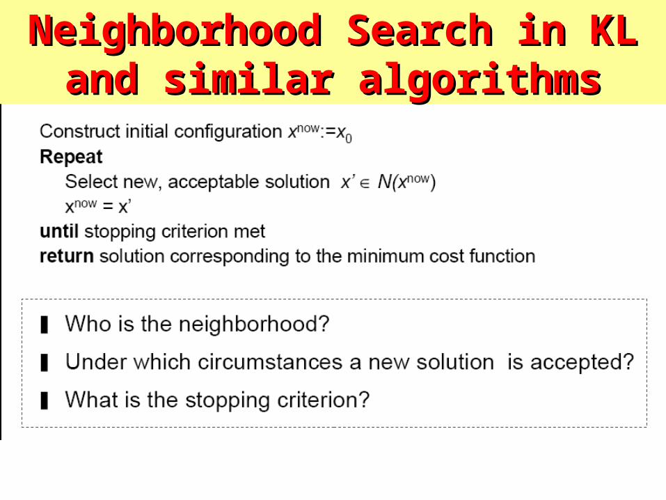
Neighborhood Search in KL and Neighborhood Search in KL and similar algorithmssimilar algorithms
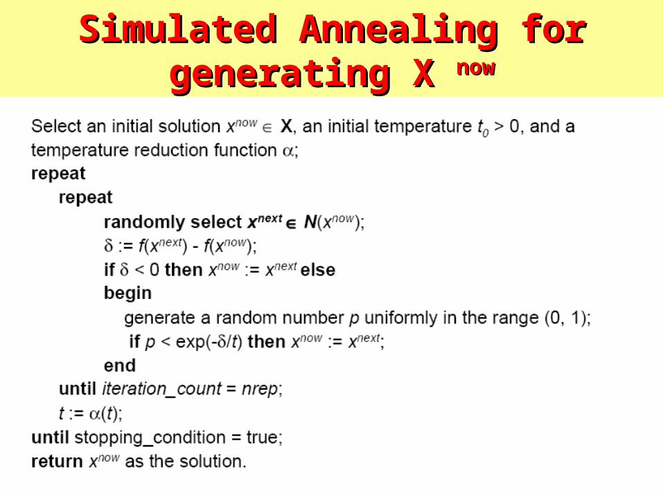
Simulated Annealing for generating Simulated Annealing for generating X X nownow
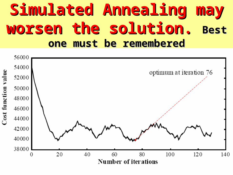
Simulated Annealing may Simulated Annealing may worsen the solution. worsen the solution. Best one must Best one must
be rememberedbe remembered

Software HardwareSoftware Hardware PartitioningPartitioning
• Hardware/software partitioning is very often treated as a particular two way partitioning in which:– performance has to be maximized and – hardware size to be minimized;
• Assumptions:– microprocessor and ASIC working in parallel;– reducing the amount of communication between the
microprocessor and the hardware coprocessor– improves the overall performance of the system.
• Objective: – Maximal performance at a given cost limit.
Hw/Sw Partitioning (cont’d)Hw/Sw Partitioning (cont’d)
• Partitioning is based on metric values derived from:– profiling, – static analysis of the specification, – and cost estimation.
• Performance improvement based on assumption that better performance is obtained if– computation intensive processes are mapped into
hardware,– parallelism is improved,– inter-domain communication is reduced

Summary on paritioning in Summary on paritioning in System level synthesisSystem level synthesis
1. The partitioning problem is NP-complete and has to be solved using optimization heuristics.
2. Partitioning heuristics are constructive or transformation based.
3.3. Hierarchical clusteringHierarchical clustering is one of the most used constructive approaches.
4. Transformational approaches are based on neighborhood search.
5. A hardware software partitioninghardware software partitioning for acceleration is done by placing computation intensive processes into hardware, improving parallelism and reducing inter-domain communication.
LiteratureLiterature
• P. Eles, K. Kuchcinski and Z. Peng, System Synthesis with VHDL, Kluwer Academic Publisher, 1998.