Embed Size (px)
Citation preview

1
2014-08-26 1
Allocation, Assignment and Scheduling
Kris Kuchcinski
2014-08-26 2
Allocation of System Components
❚ Defines an architecture by selecting hardware resources which are necessary to implement a given system.
❚ The components can be, for example, microprocessors, micro-controllers, DSP’s, ASIP’s, ASIC’s, FPGA’s, memories, buses or point-to-point links.
❚ Usually made manually with a support of estimation tools.
❚ In simple cases can be performed automatically using optimization strategy.
2014-08-26 3
Assignment of System Components
❚ After allocation the partitioning of system functionality to selected components can be done.
❚ The partitioning defines the assignment of tasks to particular components.
❚ If there is number of tasks assigned to the same component, which does not support parallel execution, the execution order need to be decided — task scheduling.
2014-08-26 4
Scheduling
❚ Depending on the computation model scheduling can be done off-line or during run-time.
❚ Static vs. dynamic scheduling.
❚ RTOS support for dynamic scheduling.
❚ Scheduling can address advanced execution techniques, such as software pipelining.
❚ Can be applied to tasks allocated to hardware, software as well as hardware operations and software instructions.
2014-08-26 5
Scheduling
❚ Data-flow scheduling (SDF, CSDF) ❙ static assignment of the instants at which the
execution takes place, ❙ time-constrained and resource-constrained, ❙ typical for DSP applications (hw and sw).
❚ Real-time scheduling ❙ periodic, aperiodic and sporadic tasks, ❙ independent or data-dependent tasks, ❙ based on priorities (static or dynamic).
2014-08-26 6
Scheduling Approaches
❚ Static scheduling ❙ static cycling scheduling
❚ Dynamic scheduling ❙ fixed priorities — e.g., rate monotonic ❙ dynamic priorities — e.g., earliest deadline first

2
Synthesis of the following code (inner loop of differential equation integrator)
while c do begin x1 := x + dx; u1 := u - ( 3 * x * u * dx) - (3 * y * dx); y1 := y + ( u * dx); c = x < a; x := x1; u := u1; y := y1; end;
7
High-Level Synthesis Scheduling
8
High-Level Synthesis Scheduling (cont’d)
3 x u dx 3 y u dx x dx
y1 c
x1 a dx y * * * *
* * u
-
u1
-
+
+
<
data-flow graph
3 x u dx 3 y u dx x dx
y1
c
x1 a
dx
* *
*
* *
* u
-
u1
- +
+
<
scheduled data-flow graph
register allocation
x u y dx
2014-08-26 9
HLS typical process
❚ Behavioral specification ❙ Language selection ❙ Parallelism ❙ Synchronization
procedure example; var a, b, c, d, e, f, g : integer; begin read(a, b, c, d, e); f := e * (a + b); g := (a + b) * (c + d); ... end;
2014-08-26 10
HLS typical process (cont’d)
❚ Design Representation ❙ parsing techniques ❙ data-flow analysis ❙ parallelism extraction ❙ program transformations
❘ elimination of high-level constructs ❘ loop unrolling ❘ subexpression detection
+
E A B C D
+
x x
F G
2014-08-26 11
HLS typical process (cont’d)
❚ Operation Scheduling ❙ Parallelism/cost trade-off ❙ Performance measure ❙ Clocking strategy +
E A B C D
+
x x
F G
2014-08-26 12
HLS typical process (cont’d)
❚ Data Path Allocation ❙ Operation selection ❙ Register/Memory allocation ❙ Interconnection Generation ❙ Hardware Minimization
3
2014-08-26 13
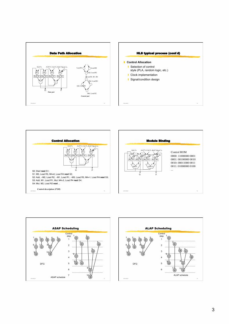
Data Path Allocation
+*
E<0:7> A<0:7> B<0:7>C<0:7> D<0:7>
FG
Reg. R1
M1
Reg. R3
M3
Reg. R4
M4
Reg. R2
M2
Data part
Load R3 Load R4
Add, Load R2
Load R1, R3, R4
Add, Load R1
Mul, Load R4
Mul, Load R2Control part
2014-08-26 14
HLS typical process (cont’d)
❚ Control Allocation ❙ Selection of control
style (PLA, random logic, etc.) ❙ Clock implementation ❙ Signal/condition design
2014-08-26 15
Control Allocation
+*
E<0:7> A<0:7> B<0:7>C<0:7> D<0:7>
FG
Reg. R1
M1
Reg. R3
M3
Reg. R4
M4
Reg. R2
M2
S0: Start next S1;"S1: M3, Load R3, M4=0, Load R4 next S2;"S2: Add, ¬M2, Load R2, ¬M1, Load R1, ¬M3, Load R3, M4=1, Load R4 next S3;"S3: Add, M1, Load R1, Mul, M4=2, Load R4 next S4;"S4: Mul, M2, Load R2 next ..."
" Control description (FSM)
2014-08-26 16
Module Binding
E<0:7> A<0:7> B<0:7>C<0:7> D<0:7>
FG
Reg. R1 Reg. R3 Reg. R4Reg. R2
Adder 8Mul 8
M1 M2 M3 M4Control ROM 0000: 11000000 0001���0001: 00100000 0010���0010: 00011000 0011���0011: 01000000 0100���...
2014-08-26 17
ASAP Scheduling
10 9
8 7 6
5 4 3 2 1 + +
+
+
-
x x
x x
DFG
+
10
9
8
7
6
5
4
3
2
1 +
+
+
+
-
x
x
x
x
+
ASAP schedule
Control step
5
4
3
2
1
6
7 2014-08-26 18
ALAP Scheduling
10 9
8 7 6
5 4 3 2 1 + +
+
+
-
x x
x x
DFG
+
10
9 8
7
6 5
4 3
2
1 +
+
+
+
-
x
x
x
x
+
ALAP schedule
Control step
5
4
3
2
1
6
4
2014-08-26 19
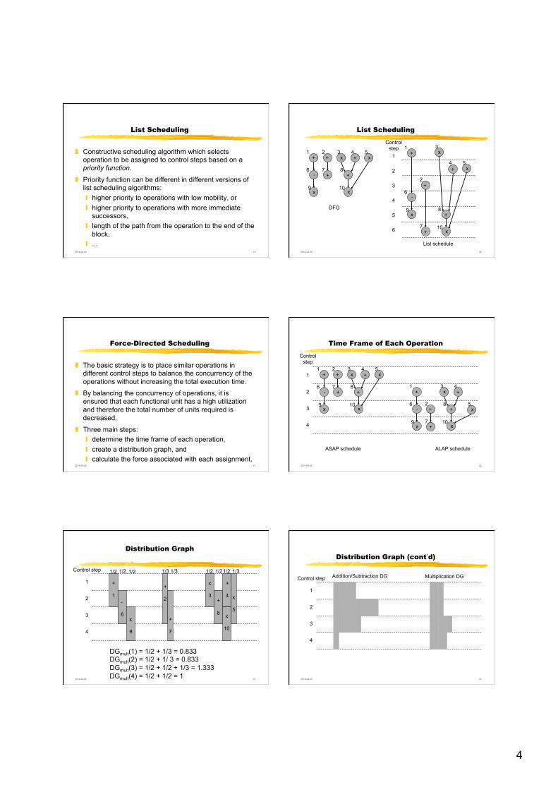
List Scheduling
❚ Constructive scheduling algorithm which selects operation to be assigned to control steps based on a priority function.
❚ Priority function can be different in different versions of list scheduling algorithms: ❙ higher priority to operations with low mobility, or ❙ higher priority to operations with more immediate
successors, ❙ length of the path from the operation to the end of the
block, ❙ ...
2014-08-26 20
List Scheduling
10 9
8 7 6
5 4 3 2 1 + +
+
+
-
x x
x x
DFG
+
10
9 8
7
6
5 4
3
2
1 +
+
+
+
-
x
x
x
x
+
List schedule
Control step
5
4
3
2
1
6
2014-08-26 21
Force-Directed Scheduling
❚ The basic strategy is to place similar operations in different control steps to balance the concurrency of the operations without increasing the total execution time.
❚ By balancing the concurrency of operations, it is ensured that each functional unit has a high utilization and therefore the total number of units required is decreased.
❚ Three main steps: ❙ determine the time frame of each operation, ❙ create a distribution graph, and ❙ calculate the force associated with each assignment.
2014-08-26 22
Time Frame of Each Operation
10 9
8 7 6
5 4 3 2 1 + +
+
+
-
x x
x x
+
Control step
4
3
2
1
ALAP schedule ASAP schedule
10 9
8
7
6 5
4 3
2
1 +
+
+
+
-
x x
x
x +
2014-08-26 23
Distribution Graph
DGmult(1) = 1/2 + 1/3 = 0.833 DGmult(2) = 1/2 + 1/ 3 = 0.833 DGmult(3) = 1/2 + 1/2 + 1/3 = 1.333 DGmult(4) = 1/2 + 1/2 = 1
Control step
4
3
2
1
1/2 1/2 1/2 1/2 1/3 1/3 1/3 1/2 1/2
+ 1
- 6
x 9
+ 2
+ 7
x 3
+ 8
+ 4
x 10
x 5
2014-08-26 24
Distribution Graph (cont’d)
Control step
4
3
2
1
Multiplication DG Addition/Subtraction DG
5
2014-08-26 25
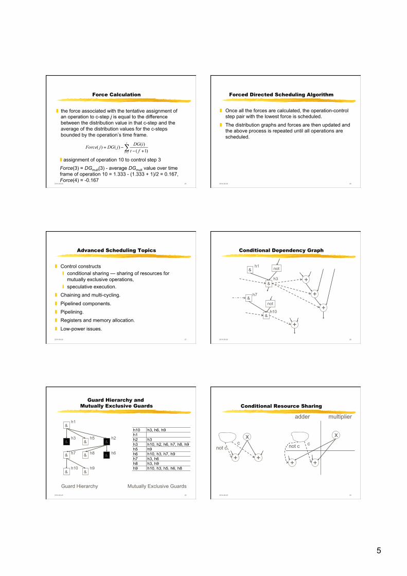
Force Calculation
❚ the force associated with the tentative assignment of an operation to c-step j is equal to the difference between the distribution value in that c-step and the average of the distribution values for the c-steps bounded by the operation’s time frame.
∑= +−
−=t
fi ftiDGjDGjForce)1()()()(
❚ assignment of operation 10 to control step 3
Force(3) = DGmult(3) - average DGmult value over time frame of operation 10 = 1.333 - (1.333 + 1)/2 = 0.167, Force(4) = -0.167
2014-08-26 26
Forced Directed Scheduling Algorithm
❚ Once all the forces are calculated, the operation-control step pair with the lowest force is scheduled.
❚ The distribution graphs and forces are then updated and the above process is repeated until all operations are scheduled.
2014-08-26 27
Advanced Scheduling Topics
❚ Control constructs ❙ conditional sharing — sharing of resources for
mutually exclusive operations, ❙ speculative execution.
❚ Chaining and multi-cycling.
❚ Pipelined components.
❚ Pipelining.
❚ Registers and memory allocation.
❚ Low-power issues.
2014-08-26 28
Conditional Dependency Graph
+
+
+
+
&
& h3
h10
&
&
h1 not
h7
not
2014-08-26 29
Guard Hierarchy and Mutually Exclusive Guards
& h1
& h3
& h5
& h2
& h7 &
h8 & h6
& h10
& h9
Guard Hierarchy Mutually Exclusive Guards
h10 h3, h6, h9h1h2 h3h3 h10, h2, h6, h7, h8, h9h5 h9h6 h10, h3, h7, h9h7 h3, h6h8 h3, h9h9 h10, h3, h5, h6, h8
& & &
&
2014-08-26 30
Conditional Resource Sharing
x
+ +
not c
c x
+ +
not c c
adder multiplier
6
2014-08-26 31
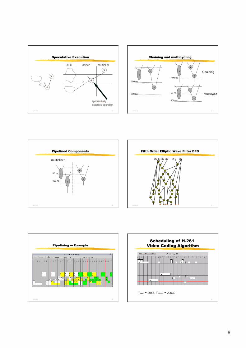
Speculative Execution
x
+
c
x
+ c
adder multiplier ALU
speculatively executed operation
2014-08-26 32
Chaining and multicycling
+
+
x
100 ns
200 ns
+
+
x
100 ns
+
+
x
100 ns
50 ns
Chaining
Multicycle
2014-08-26 33
Pipelined Components
+
+
x
100 ns
50 ns
x
multiplier 1
2014-08-26 34
Fifth Order Elliptic Wave Filter DFG
+ +
+ +
+
+ + +
+
+ +
+ + +
+ + +
+ + +
+ + + +
+
+
x x
x x
x x x
x
i1 i2 i3 i4 i5 i6
i7 i8
2014-08-26 35
Pipelining — Example
36
Scheduling of H.261 Video Coding Algorithm
Texec = 2963, T10exec = 29630
7
37
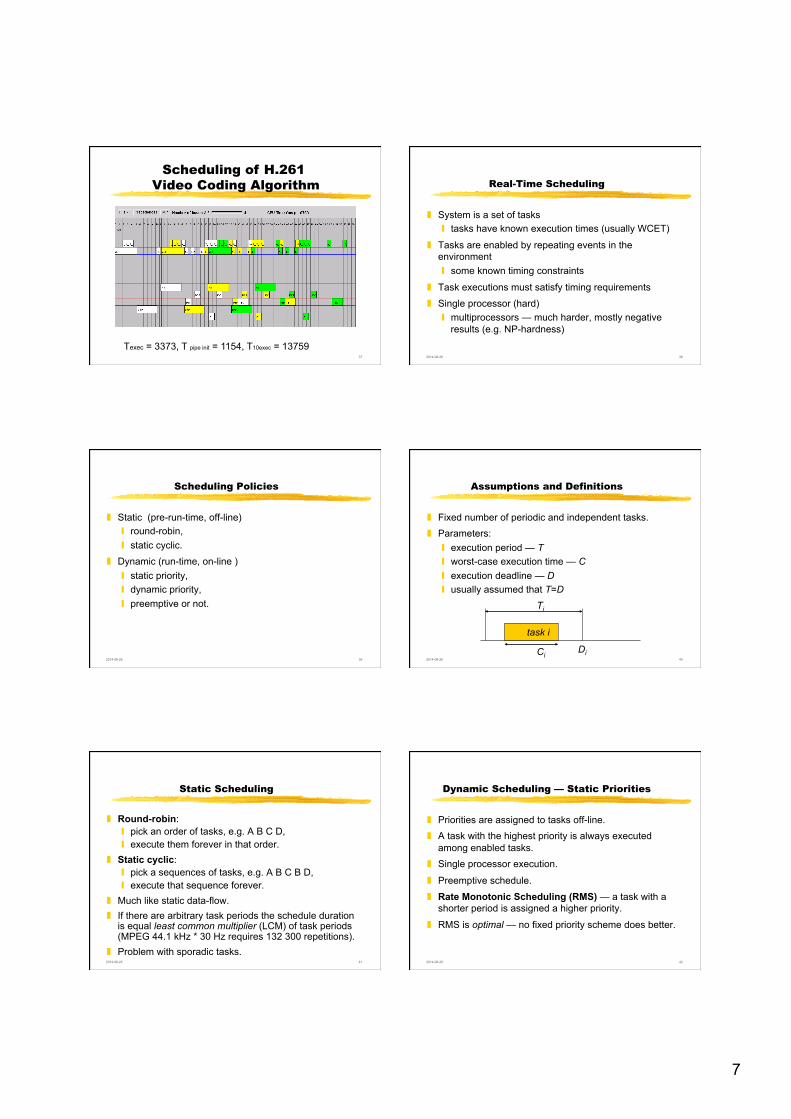
Scheduling of H.261 Video Coding Algorithm
Texec = 3373, T pipe init = 1154, T10exec = 13759 2014-08-26 38
Real-Time Scheduling
❚ System is a set of tasks ❙ tasks have known execution times (usually WCET)
❚ Tasks are enabled by repeating events in the environment ❙ some known timing constraints
❚ Task executions must satisfy timing requirements
❚ Single processor (hard) ❙ multiprocessors — much harder, mostly negative
results (e.g. NP-hardness)
2014-08-26 39
Scheduling Policies
❚ Static (pre-run-time, off-line) ❙ round-robin, ❙ static cyclic.
❚ Dynamic (run-time, on-line ) ❙ static priority, ❙ dynamic priority, ❙ preemptive or not.
2014-08-26 40
Assumptions and Definitions
❚ Fixed number of periodic and independent tasks. ❚ Parameters:
❙ execution period — T ❙ worst-case execution time — C ❙ execution deadline — D ❙ usually assumed that T=D
Ti
Ci Di
task i
2014-08-26 41
Static Scheduling
❚ Round-robin: ❙ pick an order of tasks, e.g. A B C D, ❙ execute them forever in that order.
❚ Static cyclic: ❙ pick a sequences of tasks, e.g. A B C B D, ❙ execute that sequence forever.
❚ Much like static data-flow. ❚ If there are arbitrary task periods the schedule duration
is equal least common multiplier (LCM) of task periods (MPEG 44.1 kHz * 30 Hz requires 132 300 repetitions).
❚ Problem with sporadic tasks. 2014-08-26 42
Dynamic Scheduling — Static Priorities
❚ Priorities are assigned to tasks off-line. ❚ A task with the highest priority is always executed
among enabled tasks. ❚ Single processor execution.
❚ Preemptive schedule.
❚ Rate Monotonic Scheduling (RMS) — a task with a shorter period is assigned a higher priority.
❚ RMS is optimal — no fixed priority scheme does better.
8
2014-08-26 43
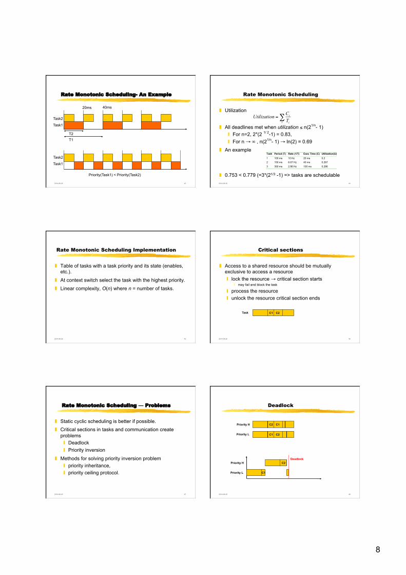
Rate Monotonic Scheduling- An Example
Task2 Task1
T2 T1
20ms 40ms
Priority(Task1) < Priority(Task2)
Task2 Task1
2014-08-26 44
Rate Monotonic Scheduling
❚ Utilization
❚ All deadlines met when utilization ≤ n(21/n- 1) ❙ For n=2, 2*(2 1/ 2-1) = 0.83, ❙ For n → ∞ , n(21/n- 1) → ln(2) = 0.69
❚ An example
❚ 0.753 < 0.779 (=3*(21/3 -1) => tasks are schedulable
∑=i i
i
TCnUtilizatio
Task Period (T) Rate (1/T) Exec Time (C) Utilization(U)
1 100 ms 10 Hz 20 ms 0.22 150 ms 6.67 Hz 40 ms 0.267
3 350 ms 2.86 Hz 100 ms 0.286
2014-08-26 45
Rate Monotonic Scheduling Implementation
❚ Table of tasks with a task priority and its state (enables, etc.).
❚ At context switch select the task with the highest priority.
❚ Linear complexity, O(n) where n = number of tasks.
2014-08-26 46
Critical sections
❚ Access to a shared resource should be mutually exclusive to access a resource ❙ lock the resource → critical section starts
❘ may fail and block the task
❙ process the resource ❙ unlock the resource critical section ends
C1 C2 Task
2014-08-26 47
Rate Monotonic Scheduling — Problems
❚ Static cyclic scheduling is better if possible. ❚ Critical sections in tasks and communication create
problems ❙ Deadlock ❙ Priority inversion
❚ Methods for solving priority inversion problem ❙ priority inheritance, ❙ priority ceiling protocol.
2014-08-26 48
Deadlock
C2 C1
C1 C2
Priority H
Priority L
Priority H
Priority L C1
C2 Deadlock
9
2014-08-26 49
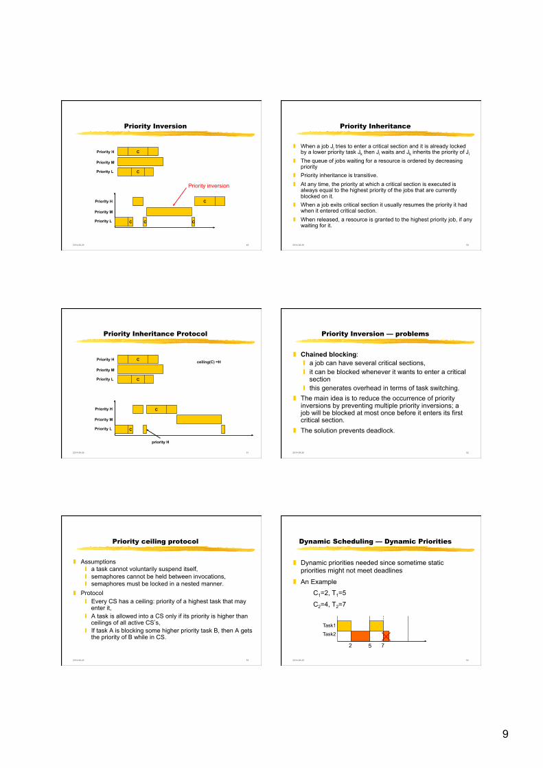
Priority Inversion
C
C
Priority H
Priority L Priority M
Priority H
Priority L Priority M
C
C
Priority inversion
C C
2014-08-26 50
Priority Inheritance
❚ When a job Ji tries to enter a critical section and it is already locked by a lower priority task Jk then Ji waits and Jk inherits the priority of Ji
❚ The queue of jobs waiting for a resource is ordered by decreasing priority
❚ Priority inheritance is transitive. ❚ At any time, the priority at which a critical section is executed is
always equal to the highest priority of the jobs that are currently blocked on it.
❚ When a job exits critical section it usually resumes the priority it had when it entered critical section.
❚ When released, a resource is granted to the highest priority job, if any waiting for it.
2014-08-26 51
Priority Inheritance Protocol
C
C
Priority H
Priority L Priority M
Priority H
Priority L Priority M
C
C
ceiling(C) =H
priority H 2014-08-26 52
Priority Inversion — problems
❚ Chained blocking: ❙ a job can have several critical sections, ❙ it can be blocked whenever it wants to enter a critical
section ❙ this generates overhead in terms of task switching.
❚ The main idea is to reduce the occurrence of priority inversions by preventing multiple priority inversions; a job will be blocked at most once before it enters its first critical section.
❚ The solution prevents deadlock.
2014-08-26 53
Priority ceiling protocol
❚ Assumptions ❙ a task cannot voluntarily suspend itself, ❙ semaphores cannot be held between invocations, ❙ semaphores must be locked in a nested manner.
❚ Protocol ❙ Every CS has a ceiling: priority of a highest task that may
enter it, ❙ A task is allowed into a CS only if its priority is higher than
ceilings of all active CS’s, ❙ If task A is blocking some higher priority task B, then A gets
the priority of B while in CS.
2014-08-26 54
Dynamic Scheduling — Dynamic Priorities
❚ Dynamic priorities needed since sometime static priorities might not meet deadlines
❚ An Example
C1=2, T1=5
C2=4, T2=7
Task1 Task2
2 5 7
10
2014-08-26 55
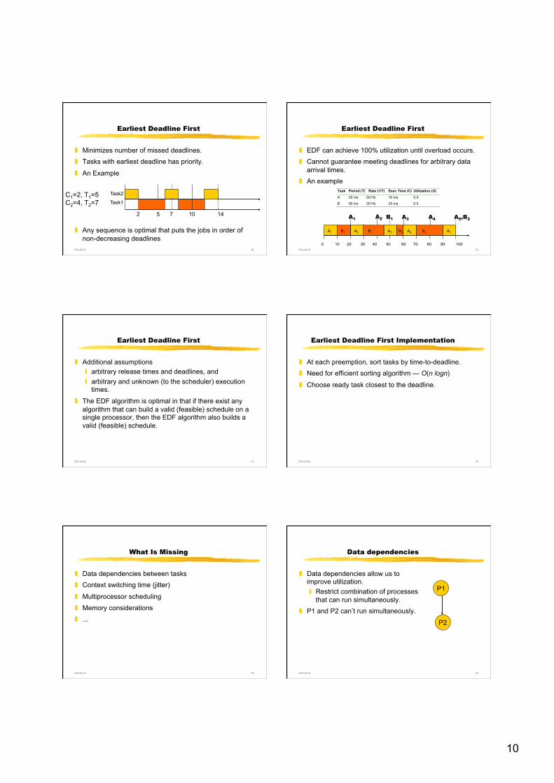
Earliest Deadline First
❚ Minimizes number of missed deadlines. ❚ Tasks with earliest deadline has priority.
❚ An Example
❚ Any sequence is optimal that puts the jobs in order of non-decreasing deadlines
Task2 Task1
2 5 7 14 10
C1=2, T1=5 C2=4, T2=7
2014-08-26 56
Earliest Deadline First
❚ EDF can achieve 100% utilization until overload occurs. ❚ Cannot guarantee meeting deadlines for arbitrary data
arrival times. ❚ An example
Task Period (T) Rate (1/T) Exec Time (C) Utilization (U)
A 20 ms 50 Hz 10 ms 0.5
B 50 ms 20 Hz 25 ms 0.5
A1 A2
0 10 20 30 40 50 60 70 80 90 100
A1 B1 A2 A3 A4 A5,B2
B1 A3 B1 B2 A4 B2 A1
2014-08-26 57
Earliest Deadline First
❚ Additional assumptions ❙ arbitrary release times and deadlines, and ❙ arbitrary and unknown (to the scheduler) execution
times.
❚ The EDF algorithm is optimal in that if there exist any algorithm that can build a valid (feasible) schedule on a single processor, then the EDF algorithm also builds a valid (feasible) schedule.
2014-08-26 58
Earliest Deadline First Implementation
❚ At each preemption, sort tasks by time-to-deadline. ❚ Need for efficient sorting algorithm — O(n logn)
❚ Choose ready task closest to the deadline.
2014-08-26 59
What Is Missing
❚ Data dependencies between tasks ❚ Context switching time (jitter)
❚ Multiprocessor scheduling
❚ Memory considerations
❚ ...
2014-08-26 60
Data dependencies
❚ Data dependencies allow us to improve utilization. ❙ Restrict combination of processes
that can run simultaneously. ❚ P1 and P2 can’t run simultaneously.
P1
P2
11
2014-08-26 61
Context-switching time
❚ Non-zero context switch time can push limits of a tight schedule.
❚ Hard to calculate effects -- depends on order of context switches.
❚ In practice, OS context switch overhead is small.
2014-08-26 62
Literature
❚ P. Eles, K. Kuchcinski and Z. Peng, System Synthesis with VHDL, Kluwer Academic Publisher, 1998.
❚ Any book on real-time scheduling, e.g., Alan Burns and Andy Wellings, Real-Time Systems and Programming Languages, Addison Wesley, 1996.