SYSC5603/ELG6163 Project Report: Implementation of an

Oversampled Subband Acoustic Echo Canceler

Brady Laska

April 2, 2007

d(n)

b(n)

v(n)y(n)+

−

d(n)

h(n) h(n)

x(n)

e(n)

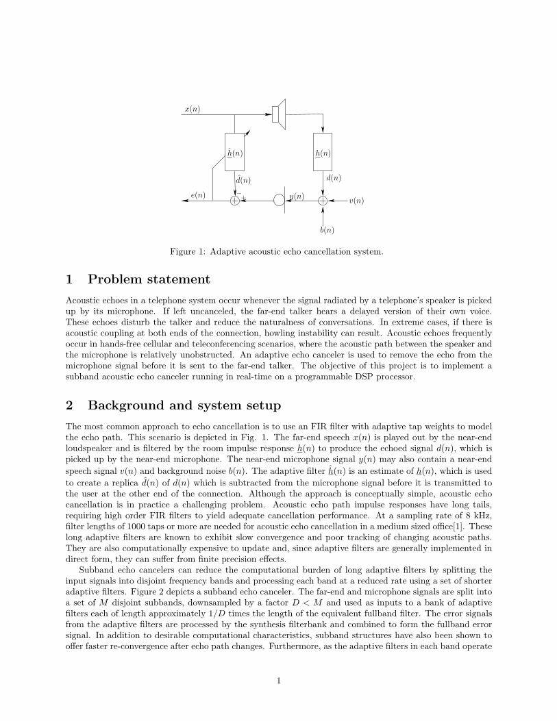
Figure 1: Adaptive acoustic echo cancellation system.

1 Problem statement

Acoustic echoes in a telephone system occur whenever the signal radiated by a telephone’s speaker is pickedup by its microphone. If left uncanceled, the far-end talker hears a delayed version of their own voice.These echoes disturb the talker and reduce the naturalness of conversations. In extreme cases, if there isacoustic coupling at both ends of the connection, howling instability can result. Acoustic echoes frequentlyoccur in hands-free cellular and teleconferencing scenarios, where the acoustic path between the speaker andthe microphone is relatively unobstructed. An adaptive echo canceler is used to remove the echo from themicrophone signal before it is sent to the far-end talker. The objective of this project is to implement asubband acoustic echo canceler running in real-time on a programmable DSP processor.

2 Background and system setup

The most common approach to echo cancellation is to use an FIR filter with adaptive tap weights to modelthe echo path. This scenario is depicted in Fig. 1. The far-end speech x(n) is played out by the near-endloudspeaker and is filtered by the room impulse response h(n) to produce the echoed signal d(n), which ispicked up by the near-end microphone. The near-end microphone signal y(n) may also contain a near-endspeech signal v(n) and background noise b(n). The adaptive filter h(n) is an estimate of h(n), which is usedto create a replica d(n) of d(n) which is subtracted from the microphone signal before it is transmitted tothe user at the other end of the connection. Although the approach is conceptually simple, acoustic echocancellation is in practice a challenging problem. Acoustic echo path impulse responses have long tails,requiring high order FIR filters to yield adequate cancellation performance. At a sampling rate of 8 kHz,filter lengths of 1000 taps or more are needed for acoustic echo cancellation in a medium sized office[1]. Theselong adaptive filters are known to exhibit slow convergence and poor tracking of changing acoustic paths.They are also computationally expensive to update and, since adaptive filters are generally implemented indirect form, they can suffer from finite precision effects.

Subband echo cancelers can reduce the computational burden of long adaptive filters by splitting theinput signals into disjoint frequency bands and processing each band at a reduced rate using a set of shorteradaptive filters. Figure 2 depicts a subband echo canceler. The far-end and microphone signals are split intoa set of M disjoint subbands, downsampled by a factor D < M and used as inputs to a bank of adaptivefilters each of length approximately 1/D times the length of the equivalent fullband filter. The error signalsfrom the adaptive filters are processed by the synthesis filterbank and combined to form the fullband errorsignal. In addition to desirable computational characteristics, subband structures have also been shown tooffer faster re-convergence after echo path changes. Furthermore, as the adaptive filters in each band operate

1

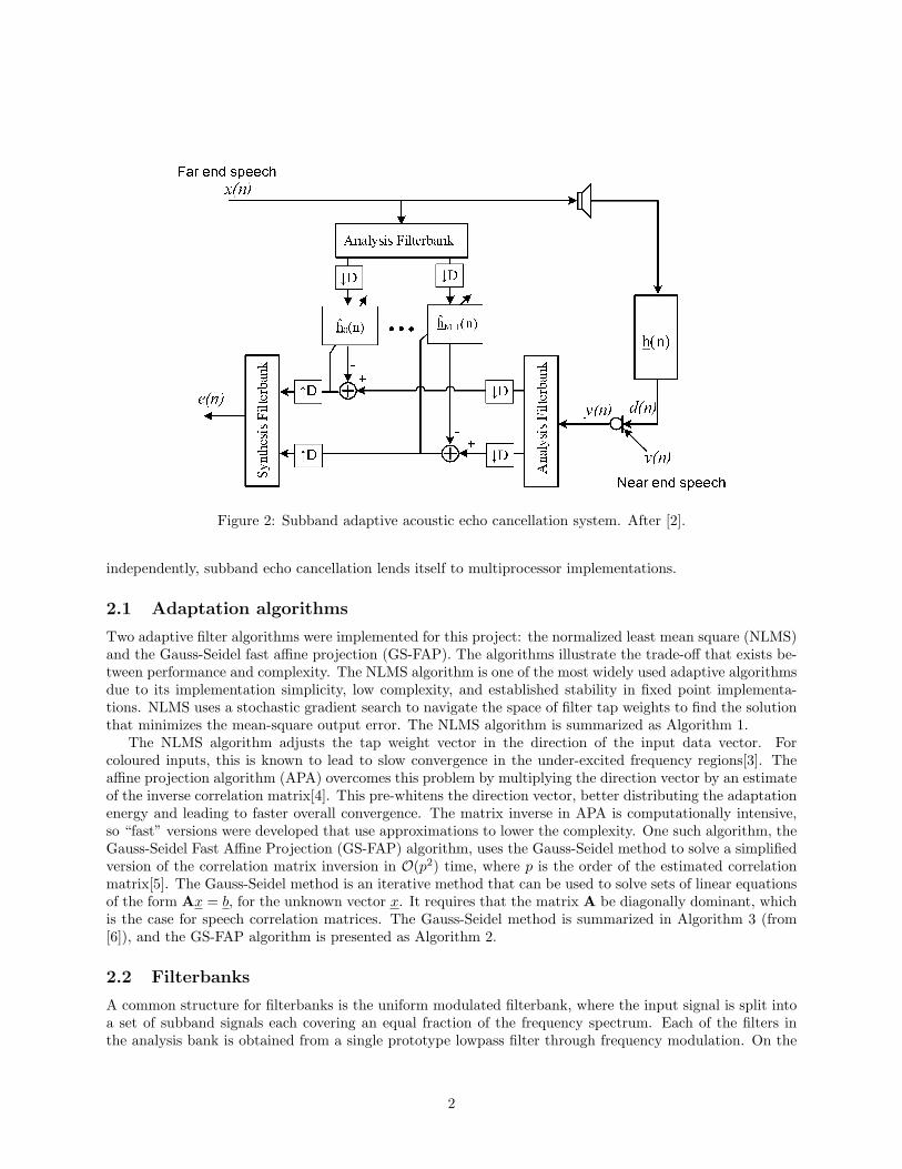
Figure 2: Subband adaptive acoustic echo cancellation system. After [2].

independently, subband echo cancellation lends itself to multiprocessor implementations.

2.1 Adaptation algorithms

Two adaptive filter algorithms were implemented for this project: the normalized least mean square (NLMS)and the Gauss-Seidel fast affine projection (GS-FAP). The algorithms illustrate the trade-off that exists be-tween performance and complexity. The NLMS algorithm is one of the most widely used adaptive algorithmsdue to its implementation simplicity, low complexity, and established stability in fixed point implementa-tions. NLMS uses a stochastic gradient search to navigate the space of filter tap weights to find the solutionthat minimizes the mean-square output error. The NLMS algorithm is summarized as Algorithm 1.

The NLMS algorithm adjusts the tap weight vector in the direction of the input data vector. Forcoloured inputs, this is known to lead to slow convergence in the under-excited frequency regions[3]. Theaffine projection algorithm (APA) overcomes this problem by multiplying the direction vector by an estimateof the inverse correlation matrix[4]. This pre-whitens the direction vector, better distributing the adaptationenergy and leading to faster overall convergence. The matrix inverse in APA is computationally intensive,so “fast” versions were developed that use approximations to lower the complexity. One such algorithm, theGauss-Seidel Fast Affine Projection (GS-FAP) algorithm, uses the Gauss-Seidel method to solve a simplifiedversion of the correlation matrix inversion in O(p2) time, where p is the order of the estimated correlationmatrix[5]. The Gauss-Seidel method is an iterative method that can be used to solve sets of linear equationsof the form Ax = b, for the unknown vector x. It requires that the matrix A be diagonally dominant, whichis the case for speech correlation matrices. The Gauss-Seidel method is summarized in Algorithm 3 (from[6]), and the GS-FAP algorithm is presented as Algorithm 2.

2.2 Filterbanks

A common structure for filterbanks is the uniform modulated filterbank, where the input signal is split intoa set of subband signals each covering an equal fraction of the frequency spectrum. Each of the filters inthe analysis bank is obtained from a single prototype lowpass filter through frequency modulation. On the

2

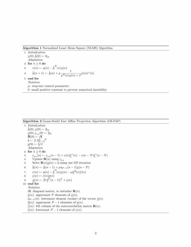
Algorithm 1 Normalized Least Mean Square (NLMS) Algorithm1: Initialization

x(0), h(0)← 0N

Adaptation2: for n ≥ 0 do3: e(n)← y(n)− h

H(n)x(n)

4: h(n + 1)← h(n) + µ1

xH(n)x(n) + δx(n)e∗(n)

5: end forNotationµ: step-size control parameter.δ: small positive constant to prevent numerical instability.

Algorithm 2 Gauss-Seidel Fast Affine Projection Algorithm (GS-FAP)1: Initialization

h(0), x(0)← 0N

η(0), rxx(0)← 0P

R(0)← δIb← [1 0T

P−1]T

p(0)← b/δAdaptation

2: for n ≥ 0 do3: rxx(n)← rxx(n− 1) + x(n)ξ∗(n)− x(n−N)ξ∗(n−N)4: Update R(n) using rxx

5: Solve R(n)p(n) = b using one GS iteration6: h(n)← h(n− 1) + µηP−1(n− 1)x(n− P )

7: e(n)← y(n)− hH(n)x(n)− µηH(n)r(n)

8: ε(n)← e(n)p(n)9: η(n)← [0 ηT (n− 1)]T + ε(n)

10: end forNotationδI: diagonal matrix, to initialize R(n).ξ(n): uppermost P elements of x(n).ηP−1(n): lowermost element (scalar) of the vector η(n).η(n): uppermost P − 1 elements of η(n).r(n): left column of the autocorrelation matrix R(n).r(n): lowermost P − 1 elements of r(n).

3

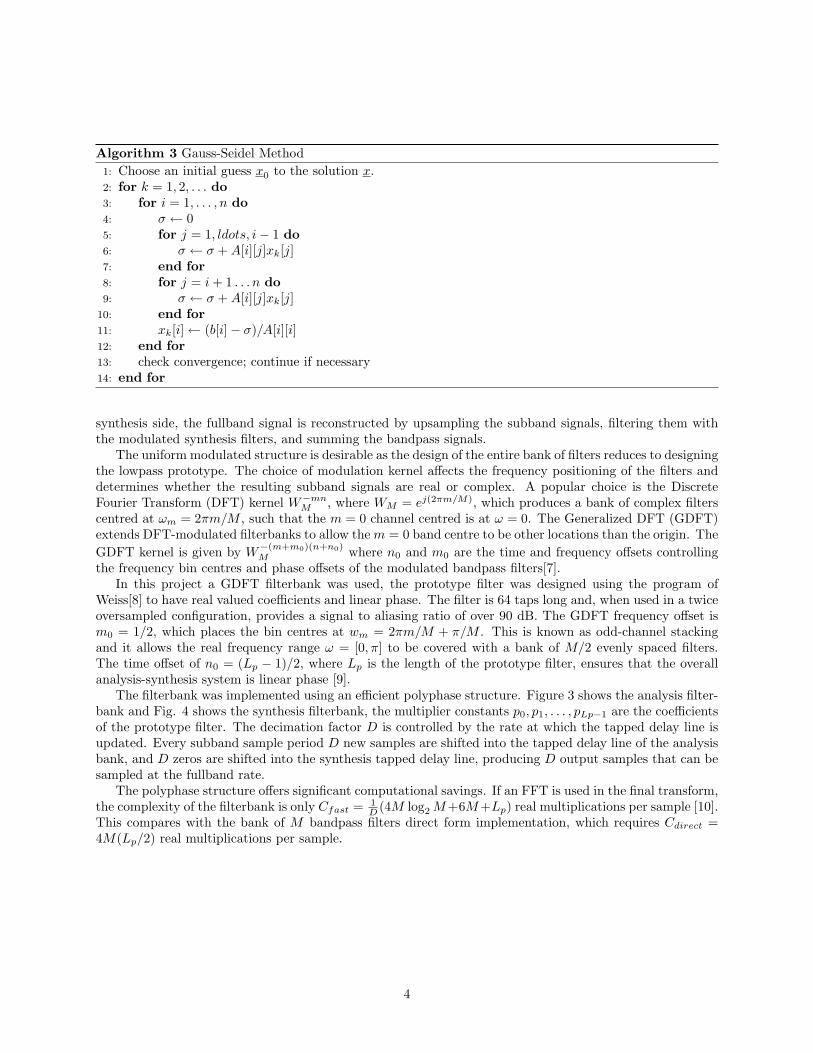
Algorithm 3 Gauss-Seidel Method1: Choose an initial guess x0 to the solution x.2: for k = 1, 2, . . . do3: for i = 1, . . . , n do4: σ ← 05: for j = 1, ldots, i− 1 do6: σ ← σ + A[i][j]xk[j]7: end for8: for j = i + 1 . . . n do9: σ ← σ + A[i][j]xk[j]

10: end for11: xk[i]← (b[i]− σ)/A[i][i]12: end for13: check convergence; continue if necessary14: end for

synthesis side, the fullband signal is reconstructed by upsampling the subband signals, filtering them withthe modulated synthesis filters, and summing the bandpass signals.

The uniform modulated structure is desirable as the design of the entire bank of filters reduces to designingthe lowpass prototype. The choice of modulation kernel affects the frequency positioning of the filters anddetermines whether the resulting subband signals are real or complex. A popular choice is the DiscreteFourier Transform (DFT) kernel W−mn

M , where WM = ej(2πm/M), which produces a bank of complex filterscentred at ωm = 2πm/M , such that the m = 0 channel centred is at ω = 0. The Generalized DFT (GDFT)extends DFT-modulated filterbanks to allow the m = 0 band centre to be other locations than the origin. TheGDFT kernel is given by W

−(m+m0)(n+n0)M where n0 and m0 are the time and frequency offsets controlling

the frequency bin centres and phase offsets of the modulated bandpass filters[7].In this project a GDFT filterbank was used, the prototype filter was designed using the program of

Weiss[8] to have real valued coefficients and linear phase. The filter is 64 taps long and, when used in a twiceoversampled configuration, provides a signal to aliasing ratio of over 90 dB. The GDFT frequency offset ism0 = 1/2, which places the bin centres at wm = 2πm/M + π/M . This is known as odd-channel stackingand it allows the real frequency range ω = [0, π] to be covered with a bank of M/2 evenly spaced filters.The time offset of n0 = (Lp − 1)/2, where Lp is the length of the prototype filter, ensures that the overallanalysis-synthesis system is linear phase [9].

The filterbank was implemented using an efficient polyphase structure. Figure 3 shows the analysis filter-bank and Fig. 4 shows the synthesis filterbank, the multiplier constants p0, p1, . . . , pLp−1 are the coefficientsof the prototype filter. The decimation factor D is controlled by the rate at which the tapped delay line isupdated. Every subband sample period D new samples are shifted into the tapped delay line of the analysisbank, and D zeros are shifted into the synthesis tapped delay line, producing D output samples that can besampled at the fullband rate.

The polyphase structure offers significant computational savings. If an FFT is used in the final transform,the complexity of the filterbank is only Cfast = 1

D (4M log2 M+6M+Lp) real multiplications per sample [10].This compares with the bank of M bandpass filters direct form implementation, which requires Cdirect =4M(Lp/2) real multiplications per sample.

4

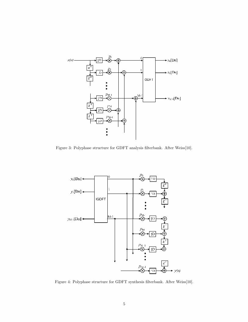
Figure 3: Polyphase structure for GDFT analysis filterbank. After Weiss[10].

Figure 4: Polyphase structure for GDFT synthesis filterbank. After Weiss[10].

5

x(n)

xM−1(Dn)

x0(Dn)

↓ D

↓ DH0(z)

HM−1(z)

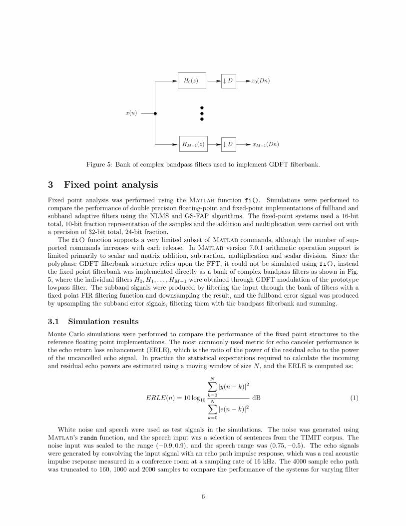
Figure 5: Bank of complex bandpass filters used to implement GDFT filterbank.

3 Fixed point analysis

Fixed point analysis was performed using the Matlab function fi(). Simulations were performed tocompare the performance of double precision floating-point and fixed-point implementations of fullband andsubband adaptive filters using the NLMS and GS-FAP algorithms. The fixed-point systems used a 16-bittotal, 10-bit fraction representation of the samples and the addition and multiplication were carried out witha precision of 32-bit total, 24-bit fraction.

The fi() function supports a very limited subset of Matlab commands, although the number of sup-ported commands increases with each release. In Matlab version 7.0.1 arithmetic operation support islimited primarily to scalar and matrix addition, subtraction, multiplication and scalar division. Since thepolyphase GDFT filterbank structure relies upon the FFT, it could not be simulated using fi(), insteadthe fixed point filterbank was implemented directly as a bank of complex bandpass filters as shown in Fig.5, where the individual filters H0,H1, . . . ,HM−1 were obtained through GDFT modulation of the prototypelowpass filter. The subband signals were produced by filtering the input through the bank of filters with afixed point FIR filtering function and downsampling the result, and the fullband error signal was producedby upsampling the subband error signals, filtering them with the bandpass filterbank and summing.

3.1 Simulation results

Monte Carlo simulations were performed to compare the performance of the fixed point structures to thereference floating point implementations. The most commonly used metric for echo canceler performance isthe echo return loss enhancement (ERLE), which is the ratio of the power of the residual echo to the powerof the uncancelled echo signal. In practice the statistical expectations required to calculate the incomingand residual echo powers are estimated using a moving window of size N , and the ERLE is computed as:

ERLE(n) = 10 log10

N∑k=0

|y(n− k)|2

N∑k=0

|e(n− k)|2dB (1)

White noise and speech were used as test signals in the simulations. The noise was generated usingMatlab’s randn function, and the speech input was a selection of sentences from the TIMIT corpus. Thenoise input was scaled to the range (−0.9, 0.9), and the speech range was (0.75,−0.5). The echo signalswere generated by convolving the input signal with an echo path impulse response, which was a real acousticimpulse rseponse measured in a conference room at a sampling rate of 16 kHz. The 4000 sample echo pathwas truncated to 160, 1000 and 2000 samples to compare the performance of the systems for varying filter

6

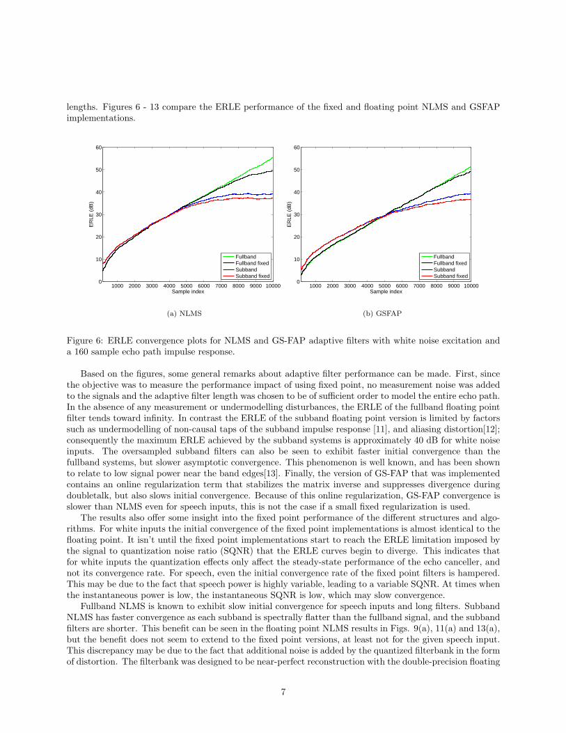
lengths. Figures 6 - 13 compare the ERLE performance of the fixed and floating point NLMS and GSFAPimplementations.

1000 2000 3000 4000 5000 6000 7000 8000 9000 100000

10

20

30

40

50

60

Sample index

ER

LE (

dB)

FullbandFullband fixedSubbandSubband fixed

(a) NLMS

1000 2000 3000 4000 5000 6000 7000 8000 9000 100000

10

20

30

40

50

60

Sample indexE

RLE

(dB

)

FullbandFullband fixedSubbandSubband fixed

(b) GSFAP

Figure 6: ERLE convergence plots for NLMS and GS-FAP adaptive filters with white noise excitation anda 160 sample echo path impulse response.

Based on the figures, some general remarks about adaptive filter performance can be made. First, sincethe objective was to measure the performance impact of using fixed point, no measurement noise was addedto the signals and the adaptive filter length was chosen to be of sufficient order to model the entire echo path.In the absence of any measurement or undermodelling disturbances, the ERLE of the fullband floating pointfilter tends toward infinity. In contrast the ERLE of the subband floating point version is limited by factorssuch as undermodelling of non-causal taps of the subband impulse response [11], and aliasing distortion[12];consequently the maximum ERLE achieved by the subband systems is approximately 40 dB for white noiseinputs. The oversampled subband filters can also be seen to exhibit faster initial convergence than thefullband systems, but slower asymptotic convergence. This phenomenon is well known, and has been shownto relate to low signal power near the band edges[13]. Finally, the version of GS-FAP that was implementedcontains an online regularization term that stabilizes the matrix inverse and suppresses divergence duringdoubletalk, but also slows initial convergence. Because of this online regularization, GS-FAP convergence isslower than NLMS even for speech inputs, this is not the case if a small fixed regularization is used.

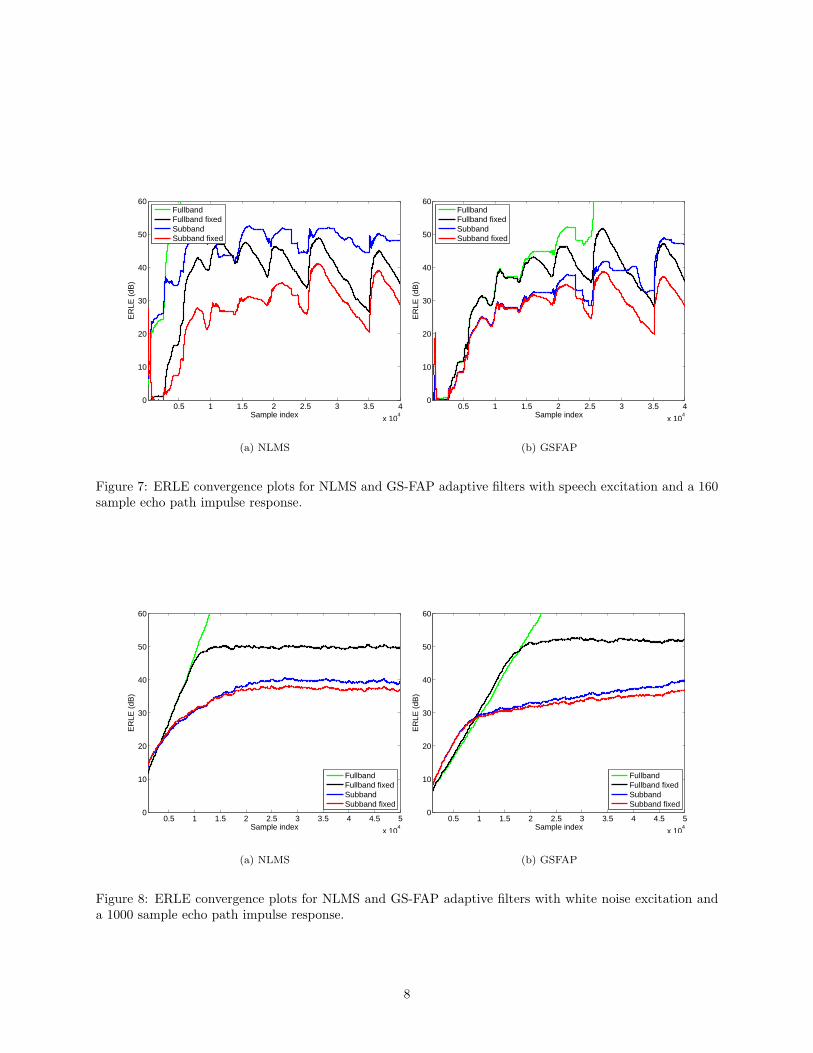
The results also offer some insight into the fixed point performance of the different structures and algo-rithms. For white inputs the initial convergence of the fixed point implementations is almost identical to thefloating point. It isn’t until the fixed point implementations start to reach the ERLE limitation imposed bythe signal to quantization noise ratio (SQNR) that the ERLE curves begin to diverge. This indicates thatfor white inputs the quantization effects only affect the steady-state performance of the echo canceller, andnot its convergence rate. For speech, even the initial convergence rate of the fixed point filters is hampered.This may be due to the fact that speech power is highly variable, leading to a variable SQNR. At times whenthe instantaneous power is low, the instantaneous SQNR is low, which may slow convergence.

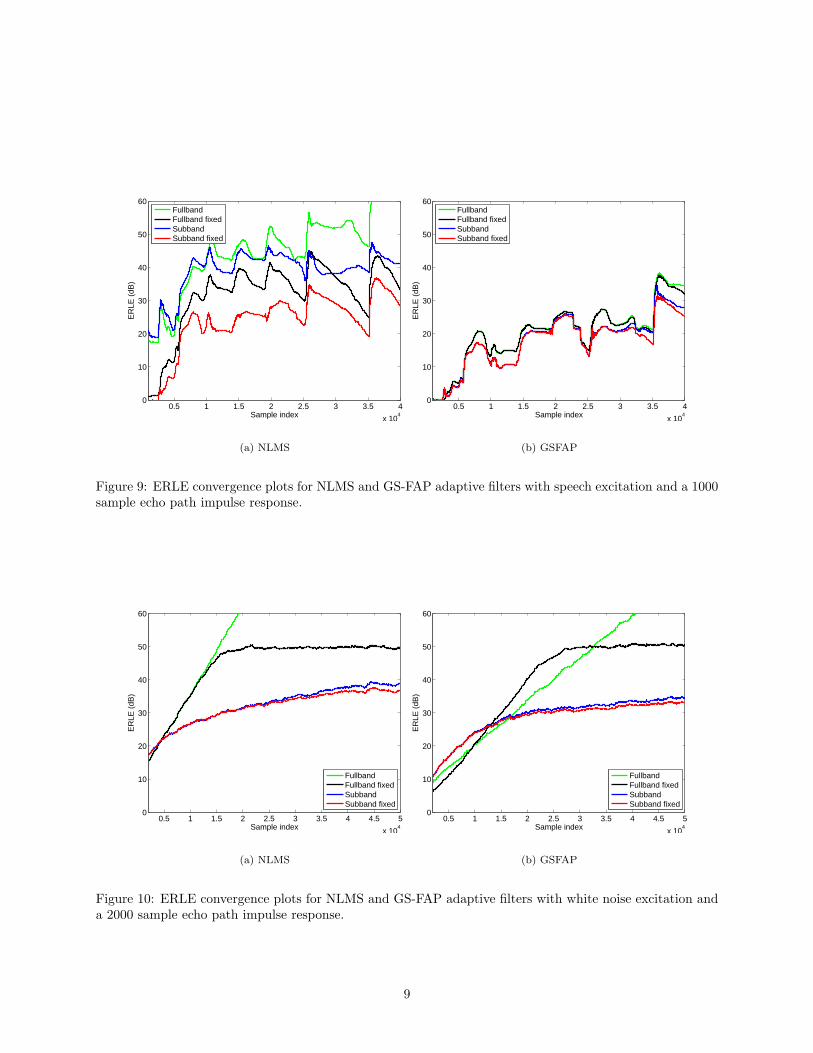
Fullband NLMS is known to exhibit slow initial convergence for speech inputs and long filters. SubbandNLMS has faster convergence as each subband is spectrally flatter than the fullband signal, and the subbandfilters are shorter. This benefit can be seen in the floating point NLMS results in Figs. 9(a), 11(a) and 13(a),but the benefit does not seem to extend to the fixed point versions, at least not for the given speech input.This discrepancy may be due to the fact that additional noise is added by the quantized filterbank in the formof distortion. The filterbank was designed to be near-perfect reconstruction with the double-precision floating

7

0.5 1 1.5 2 2.5 3 3.5 4

x 104

0

10

20

30

40

50

60

Sample index

ER

LE (

dB)

FullbandFullband fixedSubbandSubband fixed

(a) NLMS

0.5 1 1.5 2 2.5 3 3.5 4

x 104

0

10

20

30

40

50

60

Sample indexE

RLE

(dB

)

FullbandFullband fixedSubbandSubband fixed

(b) GSFAP

Figure 7: ERLE convergence plots for NLMS and GS-FAP adaptive filters with speech excitation and a 160sample echo path impulse response.

0.5 1 1.5 2 2.5 3 3.5 4 4.5 5

x 104

0

10

20

30

40

50

60

Sample index

ER

LE (

dB)

FullbandFullband fixedSubbandSubband fixed

(a) NLMS

0.5 1 1.5 2 2.5 3 3.5 4 4.5 5

x 104

0

10

20

30

40

50

60

Sample index

ER

LE (

dB)

FullbandFullband fixedSubbandSubband fixed

(b) GSFAP

Figure 8: ERLE convergence plots for NLMS and GS-FAP adaptive filters with white noise excitation anda 1000 sample echo path impulse response.

8

0.5 1 1.5 2 2.5 3 3.5 4

x 104

0

10

20

30

40

50

60

Sample index

ER

LE (

dB)

FullbandFullband fixedSubbandSubband fixed

(a) NLMS

0.5 1 1.5 2 2.5 3 3.5 4

x 104

0

10

20

30

40

50

60

Sample indexE

RLE

(dB

)

FullbandFullband fixedSubbandSubband fixed

(b) GSFAP

Figure 9: ERLE convergence plots for NLMS and GS-FAP adaptive filters with speech excitation and a 1000sample echo path impulse response.

0.5 1 1.5 2 2.5 3 3.5 4 4.5 5

x 104

0

10

20

30

40

50

60

Sample index

ER

LE (

dB)

FullbandFullband fixedSubbandSubband fixed

(a) NLMS

0.5 1 1.5 2 2.5 3 3.5 4 4.5 5

x 104

0

10

20

30

40

50

60

Sample index

ER

LE (

dB)

FullbandFullband fixedSubbandSubband fixed

(b) GSFAP

Figure 10: ERLE convergence plots for NLMS and GS-FAP adaptive filters with white noise excitation anda 2000 sample echo path impulse response.

9

0.5 1 1.5 2 2.5 3 3.5 4

x 104

0

10

20

30

40

50

60

Sample index

ER

LE (

dB)

FullbandFullband fixedSubbandSubband fixed

(a) NLMS

0.5 1 1.5 2 2.5 3 3.5 4

x 104

0

10

20

30

40

50

60

Sample indexE

RLE

(dB

)

FullbandFullband fixedSubbandSubband fixed

(b) GSFAP

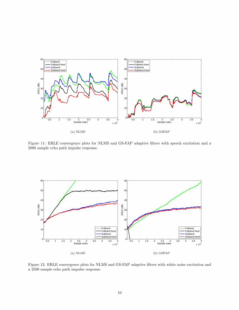
Figure 11: ERLE convergence plots for NLMS and GS-FAP adaptive filters with speech excitation and a2000 sample echo path impulse response.

0.5 1 1.5 2 2.5 3 3.5 4 4.5 5

x 104

0

10

20

30

40

50

60

Sample index

ER

LE (

dB)

FullbandFullband fixedSubbandSubband fixed

(a) NLMS

0.5 1 1.5 2 2.5 3 3.5 4 4.5 5

x 104

0

10

20

30

40

50

60

Sample index

ER

LE (

dB)

FullbandFullband fixedSubbandSubband fixed

(b) GSFAP

Figure 12: ERLE convergence plots for NLMS and GS-FAP adaptive filters with white noise excitation anda 2500 sample echo path impulse response.

10

0.5 1 1.5 2 2.5 3 3.5 4

x 104

0

10

20

30

40

50

60

Sample index

ER

LE (

dB)

FullbandFullband fixedSubbandSubband fixed

(a) NLMS

0.5 1 1.5 2 2.5 3 3.5 4

x 104

0

10

20

30

40

50

60

Sample index

ER

LE (

dB)

FullbandFullband fixedSubbandSubband fixed

(b) GSFAP

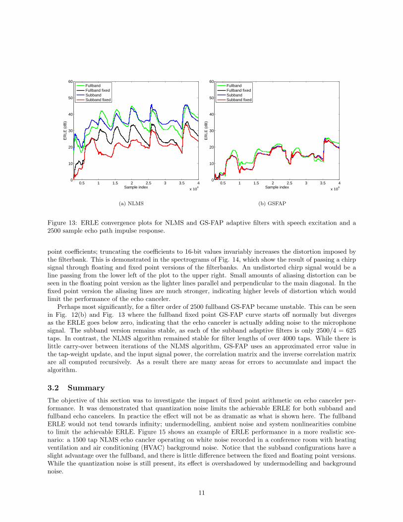
Figure 13: ERLE convergence plots for NLMS and GS-FAP adaptive filters with speech excitation and a2500 sample echo path impulse response.

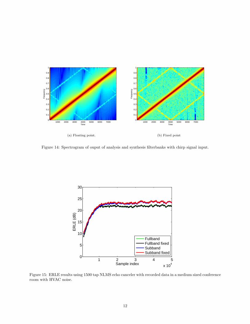
point coefficients; truncating the coefficients to 16-bit values invariably increases the distortion imposed bythe filterbank. This is demonstrated in the spectrograms of Fig. 14, which show the result of passing a chirpsignal through floating and fixed point versions of the filterbanks. An undistorted chirp signal would be aline passing from the lower left of the plot to the upper right. Small amounts of aliasing distortion can beseen in the floating point version as the lighter lines parallel and perpendicular to the main diagonal. In thefixed point version the aliasing lines are much stronger, indicating higher levels of distortion which wouldlimit the performance of the echo canceler.

Perhaps most significantly, for a filter order of 2500 fullband GS-FAP became unstable. This can be seenin Fig. 12(b) and Fig. 13 where the fullband fixed point GS-FAP curve starts off normally but divergesas the ERLE goes below zero, indicating that the echo canceler is actually adding noise to the microphonesignal. The subband version remains stable, as each of the subband adaptive filters is only 2500/4 = 625taps. In contrast, the NLMS algorithm remained stable for filter lengths of over 4000 taps. While there islittle carry-over between iterations of the NLMS algorithm, GS-FAP uses an approximated error value inthe tap-weight update, and the input signal power, the correlation matrix and the inverse correlation matrixare all computed recursively. As a result there are many areas for errors to accumulate and impact thealgorithm.

3.2 Summary

The objective of this section was to investigate the impact of fixed point arithmetic on echo canceler per-formance. It was demonstrated that quantization noise limits the achievable ERLE for both subband andfullband echo cancelers. In practice the effect will not be as dramatic as what is shown here. The fullbandERLE would not tend towards infinity; undermodelling, ambient noise and system nonlinearities combineto limit the achievable ERLE. Figure 15 shows an example of ERLE performance in a more realistic sce-nario: a 1500 tap NLMS echo cancler operating on white noise recorded in a conference room with heatingventilation and air conditioning (HVAC) background noise. Notice that the subband configurations have aslight advantage over the fullband, and there is little difference between the fixed and floating point versions.While the quantization noise is still present, its effect is overshadowed by undermodelling and backgroundnoise.

11

Time

Fre

quen

cy

1000 2000 3000 4000 5000 6000 70000

0.1

0.2

0.3

0.4

0.5

0.6

0.7

0.8

0.9

1

(a) Floating point.

Time

Fre

quen

cy

1000 2000 3000 4000 5000 6000 70000

0.1

0.2

0.3

0.4

0.5

0.6

0.7

0.8

0.9

1

(b) Fixed point

Figure 14: Spectrogram of ouput of analysis and synthesis filterbanks with chirp signal input.

1 2 3 4 5

x 104

0

5

10

15

20

25

30

Sample index

ER

LE (

dB)

FullbandFullband fixedSubbandSubband fixed

Figure 15: ERLE results using 1500 tap NLMS echo canceler with recorded data in a medium sized conferenceroom with HVAC noise.

12

4 Algorithmic transformation

The algorithmic transformation that was chosen to be implemented was unfolding. Since the target platformwas a general purpose DSP and not a hardware target the objective of unfolding was not to achieve theiteration bound, but rather to exploit instruction level parallelism in the DSP. The target processor has twosides, each with four functional units, therefore up to eight operations can be executed in parallel. Theunfolding was performed by the optimizing compiler as software pipelining. In software pipelining two ormore loop iterations are performed in parallel and independent instructions are re-ordered so that delay slotscan be filled by useful instructions. Software pipelined loops require (in general) the same number of clockcycles per iteration, but, since multiple output samples are produced in a single iteration, they require feweriterations to produce the final output. As a result the output is produced faster, and some loop branchingoverhead is saved.

The real-valued NLMS algorithm will be used as an example of software pipelining result. The mainbody of the algorithm, as listed in Algorithm 1 is in lines 3 - 4. In a C implementation, these lines wouldexpand (approximately) to the following, where N is the number of adaptive filter taps:1: for (i = 0; i < N ; i++){2: y += h[i] ·X[i] }3: e = y − y4: stepsize = µ · e5: for (i = 0; i < N ; i++) {6: h[i] += stepsize ·X[i] }

Without software pipelining or loop unrolling, these two lines from the algorithm would require 2N loopiterations to execute, even though there is no inter-iteration data dependency. Furthermore, each iterationis a multiply accumulation operation, so only one multiplication and one addition functional unit are used,leaving most of the functional units idle. This is confirmed by compiling the source without optimization.The following assembly code is a portion of the filter update step, line 6 from the above C-code:

LDW .D2T2 *+B4[0x0],B6 ; load h[i]MPYSP .M2 B8,B5,B5 ; temp = stepsize * x[i]NOP 3ADDSP .L2 B5,B6,B5 ; h[i] = h[i] + tempNOP 3STW .D2T2 B5,*+B4[0x0] ; store h[i]NOP 2LDW .D2T2 *+SP(16),B4 ;load iNOP 4ADD .D2 1,B4,B4 ; i++CMPLT .L2 B4,B9,B0 ; i < N?

[ B0] B .S1 L6 ; branchNOP 4STW .D2T2 B4,*+SP(16) ; store i

Note that no instructions are executed in parallel and that there are 16 NOP cycles, where all of thefunctional units are idle; clearly this is not an optimal use of resources. Compiling the source with theflags -o2 or -o3 passed to the optimizer enables loop unrolling and software pipelining. Since the number ofadaptive filter taps is a constant, declared in the source with a #define pre-processor statement, the compilerknows the trip count for the loops and can safely unroll them. If the number of taps were a parameter ratherthan a constant, the compiler would not software pipeline the loops unless a compiler hint such as #pragmaMUST ITERATE were placed before the loop, as the compiler would not know how far it could safely unrollthe loop. For example, if there were only 2 taps in the filter, performing 3 iterations in parallel would resultin indexing beyond array boundaries.

13

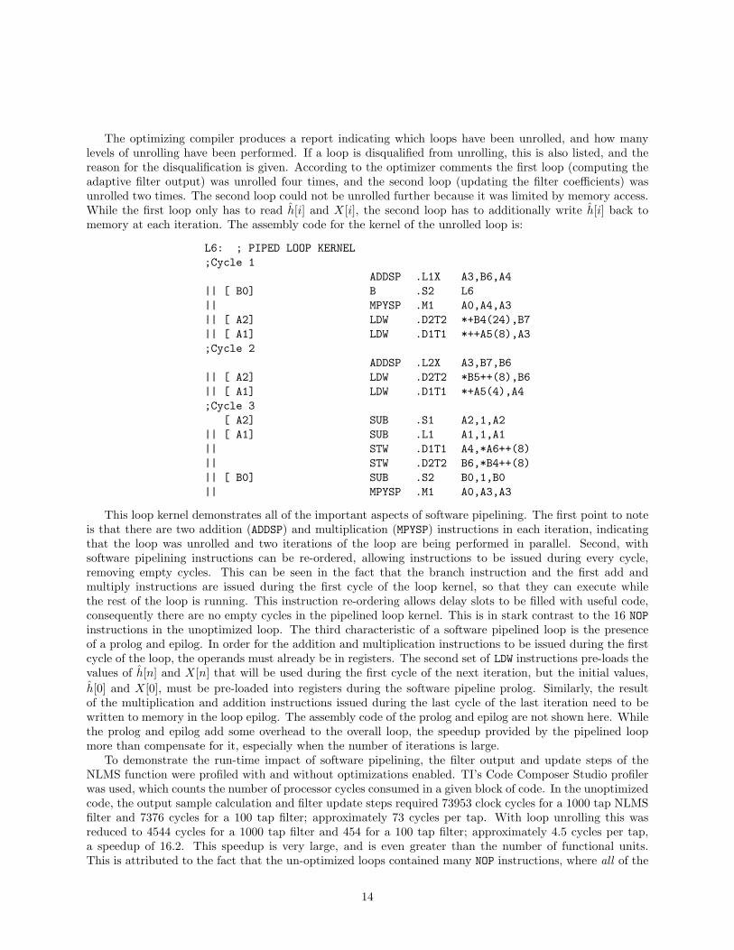
The optimizing compiler produces a report indicating which loops have been unrolled, and how manylevels of unrolling have been performed. If a loop is disqualified from unrolling, this is also listed, and thereason for the disqualification is given. According to the optimizer comments the first loop (computing theadaptive filter output) was unrolled four times, and the second loop (updating the filter coefficients) wasunrolled two times. The second loop could not be unrolled further because it was limited by memory access.While the first loop only has to read h[i] and X[i], the second loop has to additionally write h[i] back tomemory at each iteration. The assembly code for the kernel of the unrolled loop is:

L6: ; PIPED LOOP KERNEL;Cycle 1

ADDSP .L1X A3,B6,A4|| [ B0] B .S2 L6|| MPYSP .M1 A0,A4,A3|| [ A2] LDW .D2T2 *+B4(24),B7|| [ A1] LDW .D1T1 *++A5(8),A3;Cycle 2

ADDSP .L2X A3,B7,B6|| [ A2] LDW .D2T2 *B5++(8),B6|| [ A1] LDW .D1T1 *+A5(4),A4;Cycle 3

[ A2] SUB .S1 A2,1,A2|| [ A1] SUB .L1 A1,1,A1|| STW .D1T1 A4,*A6++(8)|| STW .D2T2 B6,*B4++(8)|| [ B0] SUB .S2 B0,1,B0|| MPYSP .M1 A0,A3,A3

This loop kernel demonstrates all of the important aspects of software pipelining. The first point to noteis that there are two addition (ADDSP) and multiplication (MPYSP) instructions in each iteration, indicatingthat the loop was unrolled and two iterations of the loop are being performed in parallel. Second, withsoftware pipelining instructions can be re-ordered, allowing instructions to be issued during every cycle,removing empty cycles. This can be seen in the fact that the branch instruction and the first add andmultiply instructions are issued during the first cycle of the loop kernel, so that they can execute whilethe rest of the loop is running. This instruction re-ordering allows delay slots to be filled with useful code,consequently there are no empty cycles in the pipelined loop kernel. This is in stark contrast to the 16 NOPinstructions in the unoptimized loop. The third characteristic of a software pipelined loop is the presenceof a prolog and epilog. In order for the addition and multiplication instructions to be issued during the firstcycle of the loop, the operands must already be in registers. The second set of LDW instructions pre-loads thevalues of h[n] and X[n] that will be used during the first cycle of the next iteration, but the initial values,h[0] and X[0], must be pre-loaded into registers during the software pipeline prolog. Similarly, the resultof the multiplication and addition instructions issued during the last cycle of the last iteration need to bewritten to memory in the loop epilog. The assembly code of the prolog and epilog are not shown here. Whilethe prolog and epilog add some overhead to the overall loop, the speedup provided by the pipelined loopmore than compensate for it, especially when the number of iterations is large.

To demonstrate the run-time impact of software pipelining, the filter output and update steps of theNLMS function were profiled with and without optimizations enabled. TI’s Code Composer Studio profilerwas used, which counts the number of processor cycles consumed in a given block of code. In the unoptimizedcode, the output sample calculation and filter update steps required 73953 clock cycles for a 1000 tap NLMSfilter and 7376 cycles for a 100 tap filter; approximately 73 cycles per tap. With loop unrolling this wasreduced to 4544 cycles for a 1000 tap filter and 454 for a 100 tap filter; approximately 4.5 cycles per tap,a speedup of 16.2. This speedup is very large, and is even greater than the number of functional units.This is attributed to the fact that the un-optimized loops contained many NOP instructions, where all of the

14

functional units were idle.

5 Implementation results

5.1 Implementation platform

The DSP processor chosen for the implementation was the Texas Instruments TMS320C6713 floating pointDSP. The C6713 is a very large instruction word (VLIW) processor with two sides each containing fourfunctional units. The processor operates at a clock speed of 225 MHz, and its eight functional units enableexecution of up to 1350 million floating-point operations per second (MFLOPS) [14]. A wideband echocanceler operating at a sampling rate of 16 kHz would therefore be able to perform over 84000 floating pointoperations per sample. Imperfect compilers, data dependencies and program branches mean that the fullparallel execution potential of the processor will not be realized in practice, so not all of the functional unitswill be executing an instruction at every clock cycle and the actual rate of operations will be lower thanthe theoretical maximum. However, even operating below its theoretical potential, the C6713 has sufficientprocessing power to execute sophisticated adaptation algorithms on long adaptive filters in real-time.

5.2 Compiled Simulink model

The original implementation strategy for this project called for producing C-code by directly compilingSimulink models using the “Embedded Target for C6000” toolbox. As discussed in the interim report, thismethod proved to be impractical. The generated code exhibited a high level of abstraction, each Simulinkblock was treated as a distinct object with input and output buffers. This resulted in a great deal of inter-block communication, and a large computational overhead. Furthermore, the structure of the generated codemade it difficult, if not impossible, to hand optimize without breaking the program.

It should be noted that while it was not practical in this case, compiling directly from Simulink modelsto an embedded target may be possible in some situations. If a designer has a Simulink model with customblocks written in C it would be possible to perform rapid prototyping using this approach. The codegeneration tools would handle the interfacing between the blocks, making it easy to vary system parametersand interchange algorithm blocks. While the general Real-Time Workshop compiler does not seem suitedto producing production-level code, the Mathworks offers an additional toolbox that is designed for thispurpose, the Real-Time Embedded Coder. According to the documentation “the Real-Time WorkshopEmbedded Coder provides a framework for the development of production code that is optimized for speed,memory usage, and simplicity. The Real-Time Workshop Embedded Coder is intended for use in embeddedsystems”[15]. By simplifying the calling interface, inlining S-functions, performing static memory allocationand other optimizations, the overhead of the code is reduced, making automatic generation of productioncode possible.

5.3 Hand written C-code

While the hand written C-code was designed to be run in real-time, some optimizations were sacrificed inorder to keep the implementation flexible. Since fullband and subband versions of NLMS and GS-FAP wereimplemented, the code was written in modules with some degree of abstraction to facilitate easy changing ofthe echo canceler structure, the adaptation algorithm and the algorithm parameters. A more performanceoriented approach would have limited the number of function calls, and might have made more use of globalvariables to reduce the number of parameters passed to functions. In order to make the code easy to readand write, the tapped delay line data buffers were implemented as arrays and were updated by shufflingthe previous values down the array and adding the new value at index 0. This implementation is clearlyinefficient as it requires O(N) operations to update a buffer of size N , rather than the O(1) operationsrequired if circular buffers were used.

15

Complex math operations were written in-line, and real and imaginary parts of complex values wereinterleaved in matrices and vectors. This approach, while good for performance, made debugging verydifficult. Further object orientation using complex data types with operator overloading could have madethe code easier to read and debug.

The filterbank code was a slightly modified version of the reference code available from [8]. The codewas intended to demonstrate the behaviour of the polyphase filterbank and was written for reading clarityrather than performance. To increase the performance the code could be refactored to reduce the number oftemporary variables used (decrease register usage) and to reduce the number of function calls. The code wasalso written to work for an arbitrary number of subbands and for any decimation factor. Operations suchas the FFT routine could be optimized for a given number of subbands and decimation factor, to furtherincrease the performance.

Two different versions of the final program were produced. One version polled the ADC and DAC to readand write one sample of data at a time, the other version used frame-based EDMA for much more efficientdata transfer. The EDMA code used TI’s reference program “dsk app”, which uses double buffering andEDMA transfers to minimize the data transfer overhead. The polling version was especially inefficient forthe subband implementations. With a decimation factor of 4, the processor was idle until 4 samples wereaccumulated by polling, at which point the subband analysis, adaptive filter update and fullband synthesissteps were performed. While the overall processor utilization may have been less than the fullband case,the utilization was very bursty and the peak requirement was higher than the fullband filter’s constantrequirement.

5.4 Performance and bottleneck

Compiling the code with optimizations disabled (no software pipelining) produced a program that couldperform real-time echo cancellation at 8 kHz using a 300 tap adaptive filter. Increasing the sampling rate orthe number of taps caused frames to be dropped resulting in pops at the output and misconvergence of theadaptive filter. Enabling software pipelining allowed a 1000 tap NLMS adaptive filter to run in real-time at32 kHz. Even at this rate, which is twice the sampling rate used for “wideband” telephony, the processorutilization, as reported by the DSP-BIOS CPU monitior, was only 86%. A reasonable target for an acousticecho canceler is modelling a 250 ms echo path. At 8 kHz, standard telephony sampling rate, this correspondsto a 2000 tap filter. Using the EDMA code with these parameters, fullband NLMS consumes approximately43% of the processor resources, and fullband GS-FAP consumes approximately 35%. It is surprising thatGS-FAP has lower processor utilization that NLMS, as GS-FAP requires many more operations per samplethan NLMS. One possible reason for the difference is that GS-FAP updates the tap-weight vector at time nusing the error value from time n−1. In contrast, NLMS uses the error value from time n, so the error mustbe computed before the tap weights can be updated. Consequently GS-FAP can perform the tap-weightupdate and error output computations in the same loop, while NLMS requires two separate loops; this mayallow GS-FAP to make better use of the VLIW parallelism. For both algorithms it is clear that the chosenprocessor is powerful enough to perform real-time echo cancellation, possibly in addition to tasks such asspeech coding.

Profiling revealed that, as expected, the bottleneck in the implementation is loops required to computethe filter output and update the adaptive filter. Other than software pipelining there is little that can be doneto alleviate this bottleneck; for a real adaptive filter of length N , at least N multiplications and additionsneed to be performed in order to compute the output and update the filter. More sophisticated algorithmsrequire even more computations. Hand coded assembly may be able to make more efficient use of registersand avoid some memory operations, but most of the attainable performance is achieved by the optimizingcompiler.

Some minor changes could be made to speed up the code. As mentioned the the previous section, someperformance was sacrificed in the interest of flexibility and code readibility. For example, with an order Nadaptive filter, the use of a circular input signal buffer would save approximately N operations comparedto the existing implementation. There is also overhead involved in getting samples from ADC. Using larger

16

data frames could reduce this overhead, but larger frames also increase the delay in the signal path, whichis undesireable in telephony applications.

6 Conclusion and Discussion

The goal of this project was achieved. Working fullband and subband adaptive echo cancelers using NLMSand GSFAP, were implemented and are able to run in real-time on a programmable floating point DSP.Furthermore, fixed point analysis indicates that a fixed point implementation of these algorithms would befeasible for a fullband or subband configuration, depending on the length of the echo path to be modelled.

Adaptive filtering algorithms are generally quite computationally intensive, but their operations arerepetitive and very amenable to software pipelining. It was demonstrated that unfolding (loop unrolling)can drastically improve the performance, significantly increasing the length of adaptive filter that can beused in a real-time implementation.

The echo reduction performance of the subband systems was lower than the equivalent fullband filter,and the difference was greater for the fixed point implementation than the floating point. This is attributedto the previously studied limitations of subband systems[12], and to the additional distortion imposed bythe fixed-point filterbank. Performance may be improved if the filterbank were designed with fixed pointconsiderations in mind rather than the current implementation which simply truncated double precisioncoefficients. Subband GS-FAP was however shown to be more robust to finite precision effects than fullband.Fixed point fullband GS-FAP became unstable in modelling an echo path that was 2500 samples long. Fora given echo path length each of the subband filters are significantly shorter than the fullband filter, solonger echo paths can be modelled by subband adaptive filters without incurring instability. On the otherhand, fixed point fullband and subband NLMS remained stable even for echo path lengths of 4000 samples.This robust fixed point performance is a primary reason why NLMS is frequently used in adaptive filters inpractice.

Appendix

The C and Matlab code, and all of the Simulink models used in this project are included as an attachmentto the soft copy of this report.

17

References

[1] C. Breining, P. Dreiscitel, E. Hansler, A. Mader, B. Nitsch, H. Puder, T. Schertler, G. Schmidt, andJ. Tilp, “Acoustic echo control. An application of very-high-order adaptive filters,” IEEE Signal Pro-cessing Mag., vol. 16, pp. 42 – 69, July 1999.

[2] J. J. Shynk, “Frequency-domain and multirate adaptive filtering,” IEEE Signal Processing Mag., vol. 9,pp. 14 – 37, Jan. 1992.

[3] D. T. Slock, “On the convergence behavior of the LMS and the normalized LMS algorithms,” IEEETransactions on Signal Processing, vol. 41, no. 9, pp. 2811 – 2825, 1993.

[4] K. Ozeki and T. Umeda, “An adaptive filtering algorithm using an orthogonal projection to an affinesubspace and its properties,” Electronics and Communications in Japan (English translation of DenshiTsushin Gakkai Zasshi), vol. 67, no. 5, pp. 19 – 27, 1984.

[5] F. Albu, J. Kadlec, N. Coleman, and A. Fagan, “The Gauss-Seidel fast affine projection algorithm,”IEEE Workshop on Signal Processing Systems (SPIS’02), pp. 109 – 14, 2002.

[6] R. Barrett and M. B. et. al, Templates for the Solution of Linear Systems: Building Blocks for IterativeMethods. Society for Industrial and Applied Mathematics, 1994.

[7] R. E. Crochiere and L. R. Rabiner, Multirate Digital Signal Processing. Prentice Hall, 1983.

[8] S. Weiss, “Filter banks.” Online at http://www.ecs.soton.ac.uk/~sw1/software/software.html,Jan 2001.

[9] M. Harteneck, S. Weiss, and R. W. Stewart, “Design of near perfect reconstruction oversampled filterbanks for subband adaptive filters,” IEEE Transactions on Circuits and Systems II: Analog and DigitalSignal Processing, vol. 46, no. 8, pp. 1081 – 1085, 1999.

[10] S. Weiss, L. Lampe, and R. Stewart, “Efficient implementations of complex and real valued filter banksfor comparative subband processing with an application to adaptive filtering,” Proceedings of FirstInternational Symposium on Communication Systems and Digital Signal Processing, vol. 1, pp. 32 – 5,1998.

[11] W. Kellermann, “Analysis and design of multirate systems for cancellation of acoustical echoes,” inProc. IEEE ICASSP ’88, vol. 5, pp. 2570 – 2573, Apr. 1988.

[12] S. Weiss, A. Stenger, R. Stewart, and R. Rabenstein, “Steady-state performance limitations of subbandadaptive filters,” IEEE Transactions on Signal Processing, vol. 49, pp. 1982 – 91, September 2001.

[13] D. Morgan, “Slow asymptotic convergence of LMS acoustic echo cancelers,” IEEE Transactions onSpeech and Audio Processing, vol. 3, no. 2, pp. 126 – 36, 1995/03/.

[14] TI Techinical Staff, “TMS320C6713 floating point digital signal processor,” Tech. Rep. SPRS186L,Texas Instruments, Nov. 2005.

[15] Mathworks Technical Staff, “Real-time workshop embedded coder,” Tech. Rep. Document version 3.2.1,The Mathworks, Oct. 2004.

18