Embed Size (px)
Citation preview
Polynomial Interpolators forHigh-Quality Resampling ofOversampled Audio
by Olli Niemitalo in August 2001. Distribute, host and use this paper freely.http://www.student.oulu.fi/~oniemita/DSP/INDEX.HTM
Abstract
This paper discusses piece-wise polynomial interpolators used in audio resam-pling and presents new low-order designs that are optimized for high-quality re-sampling of oversampled audio. Source code and useful tables for using theinterpolators are included.
Welcome to read the paper that took three entire weeks (24/7) of my life, approximately 11000 of
the whole deal. It was a very educational experience. I learned to play with genetic algorithms(big thanks to Bram de Jong for introducing Differential Evolution, which was also used in gen-eration of the passband approximations, and to Robert Bristow-Johnson, whose AES paper withDuane Wise, "Performance of Low-Order Polynomial Interpolators in the Presence of Oversam-pled Input", this one owes a lot to). And I learned a new language, PostScript, which was used togenerate the graphs directly from a C++ program. And I got more and more familiar with LATEX. Alsosome pretty nice interpolators were generated, and I’m sure to be using them in the future. I couldeasily say I need a short break from interpolation, but I won’t because that’s such an over-usedclosing joke.
You may notice that there aren’t any references. The additional bits of information for creating thispaper were gathered from Internet exclusively, and most of the sources were not named publica-tions. So if you wish to find them, just figure out a few keywords and head to http://www.google.com.
You are very welcome to send error reports/comments/opinions/announcements of implementa-tions/work offers/free audio software/anything except viruses/spam to my e-mail (under the title).
1
CONTENTS 2
Contents
1. Introduction . . . . . . . . . . . . . . . . . . . . . . . . . . . . . . . 3
2. A bunch of interpolators . . . . . . . . . . . . . . . . . . . . . . . . 52.1 Drop-sample, linear, B-spline . . . . . . . . . . . . . . . . . 52.2 Lagrange . . . . . . . . . . . . . . . . . . . . . . . . . . . . 82.3 Hermite (1st-order-osculating) . . . . . . . . . . . . . . . . 102.4 2nd-order-osculating . . . . . . . . . . . . . . . . . . . . . . 122.5 Watte tri-linear and "parabolic 2x" . . . . . . . . . . . . . . 14
3. A quality measure . . . . . . . . . . . . . . . . . . . . . . . . . . . 16
4. New optimal designs . . . . . . . . . . . . . . . . . . . . . . . . . . 184.1 2-point, 3rd-order optimal . . . . . . . . . . . . . . . . . . . 184.2 4-point, 2nd-order optimal . . . . . . . . . . . . . . . . . . . 204.3 4-point, 3rd-order optimal . . . . . . . . . . . . . . . . . . . 214.4 4-point, 4th-order optimal . . . . . . . . . . . . . . . . . . . 234.5 6-point, 4th-order optimal . . . . . . . . . . . . . . . . . . . 244.6 6-point, 5th-order optimal . . . . . . . . . . . . . . . . . . . 26
5. Comparison . . . . . . . . . . . . . . . . . . . . . . . . . . . . . . . 285.1 Linear . . . . . . . . . . . . . . . . . . . . . . . . . . . . . . 285.2 B-spline . . . . . . . . . . . . . . . . . . . . . . . . . . . . . 295.3 Lagrange . . . . . . . . . . . . . . . . . . . . . . . . . . . . 295.4 Hermite . . . . . . . . . . . . . . . . . . . . . . . . . . . . . 305.5 2nd-order-osculating . . . . . . . . . . . . . . . . . . . . . . 315.6 Watte tri-linear . . . . . . . . . . . . . . . . . . . . . . . . . 325.7 Parabolic 2x . . . . . . . . . . . . . . . . . . . . . . . . . . 325.8 Optimal . . . . . . . . . . . . . . . . . . . . . . . . . . . . . 32
6. Implementation . . . . . . . . . . . . . . . . . . . . . . . . . . . . . 346.1 Linear . . . . . . . . . . . . . . . . . . . . . . . . . . . . . . 376.2 B-spline . . . . . . . . . . . . . . . . . . . . . . . . . . . . . 376.3 Lagrange . . . . . . . . . . . . . . . . . . . . . . . . . . . . 396.4 Hermite . . . . . . . . . . . . . . . . . . . . . . . . . . . . . 406.5 2nd-order-osculating . . . . . . . . . . . . . . . . . . . . . . 436.6 Watte tri-linear . . . . . . . . . . . . . . . . . . . . . . . . . 456.7 Parabolic 2x . . . . . . . . . . . . . . . . . . . . . . . . . . 466.8 2-point, 3rd-order optimal . . . . . . . . . . . . . . . . . . . 466.9 4-point, 2nd-order optimal . . . . . . . . . . . . . . . . . . . 486.10 4-point, 3rd-order optimal . . . . . . . . . . . . . . . . . . . 496.11 4-point, 4th-order optimal . . . . . . . . . . . . . . . . . . . 506.12 6-point, 4th-order optimal . . . . . . . . . . . . . . . . . . . 516.13 6-point, 5th-order optimal . . . . . . . . . . . . . . . . . . . 53
7. Summary . . . . . . . . . . . . . . . . . . . . . . . . . . . . . . . . 55
8. Pre-emphasis . . . . . . . . . . . . . . . . . . . . . . . . . . . . . . 57
9. Conclusion . . . . . . . . . . . . . . . . . . . . . . . . . . . . . . . 60

1. Introduction 3
1. Introduction
Sampled audio data is a discrete-time representation of a continuous signal, per-haps of the voltage that came from the microphone while recording. As a rule,the data holds the amplitude values of the continuous signal at the boundariesof evenly spaced time intervals. To change the sampling frequency by an uncon-strained ratio – a common task in audio processing – or to create sub-samplelength delays, both a form of resampling, one needs to be able to read the con-tinuous signal between the samples.
The solution is to create an approximation of the continuous signal, from the in-formation contained in the samples, and to sample that. This is called interpola-tion, finding the function value between known samples. A common interpolationmethod is linear interpolation, where the continuous function is approximated aspiece-wise-linear by drawing lines between the successive samples. An evenmore crude form of interpolation is drop-sample interpolation, drawing a horizon-tal line from each sample until the following sample.
Drop-sample and linear interpolation (as such) are not adequate for high-qualityresampling, but even linear interpolation is a big improvement compared to drop-sample. Both of them fall into the category of piece-wise polynomial interpolators.Theoretically, one could create a very high-order polynomial interpolator and getthe desired quality. A rule of thumb was formed from the results of this paper:The dependence, of the interpolation error in dB scale and the computationalcomplexity of a good polynomial interpolator, is a linear function with an offset.Unfortunately, the function is relatively gently sloping, so the polynomial orderwould need to be increased to something unreasonable to get transparent quality.
A hybrid solution is to first oversample the input by a simple ratio using discretemethods and then interpolate this oversampled data using a polynomial interpo-lator. When a symmetrical FIR is used as the discrete oversampling filter, peopleoften call the method sinc interpolation, especially if the oversampling ratio islarge, which makes the FIR lowpass coefficient table resemble a windowed sincand the impulse response of the whole hybrid interpolator a piece-wise polynomialapproximation of a windowed sinc. The exact same results can be achieved dif-ferently, by interpolating the FIR coefficient table with the polynomial interpolatorand by filtering using the interpolated coefficients, but this approach is computa-tionally more expensive and not suggested.
This paper concentrates on improving the polynomial interpolation stage of thehybrid method, for oversampling ratios of 2, 4, 8, 16 and 32 on the oversamplingstage.
A discrete oversampling filter can increase the sampling frequency to an integerN multiple, i.e. oversample by N. Typically, the filter is a FIR filter, because usinga FIR one can do "random access" on the data with no extra computational cost– a useful property if N is high, because in such cases typically only a fractionof the samples in the oversampled signal are used. Another recent solution is a
1. Introduction 4
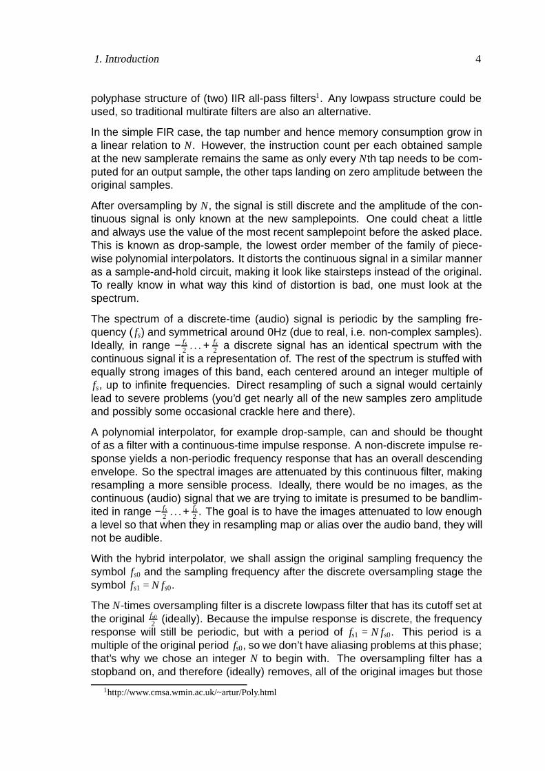
polyphase structure of (two) IIR all-pass filters1. Any lowpass structure could beused, so traditional multirate filters are also an alternative.
In the simple FIR case, the tap number and hence memory consumption grow ina linear relation to N. However, the instruction count per each obtained sampleat the new samplerate remains the same as only every Nth tap needs to be com-puted for an output sample, the other taps landing on zero amplitude between theoriginal samples.
After oversampling by N, the signal is still discrete and the amplitude of the con-tinuous signal is only known at the new samplepoints. One could cheat a littleand always use the value of the most recent samplepoint before the asked place.This is known as drop-sample, the lowest order member of the family of piece-wise polynomial interpolators. It distorts the continuous signal in a similar manneras a sample-and-hold circuit, making it look like stairsteps instead of the original.To really know in what way this kind of distortion is bad, one must look at thespectrum.
The spectrum of a discrete-time (audio) signal is periodic by the sampling fre-quency ( fs) and symmetrical around 0Hz (due to real, i.e. non-complex samples).Ideally, in range − fs
2 . . . + fs
2 a discrete signal has an identical spectrum with thecontinuous signal it is a representation of. The rest of the spectrum is stuffed withequally strong images of this band, each centered around an integer multiple offs, up to infinite frequencies. Direct resampling of such a signal would certainlylead to severe problems (you’d get nearly all of the new samples zero amplitudeand possibly some occasional crackle here and there).
A polynomial interpolator, for example drop-sample, can and should be thoughtof as a filter with a continuous-time impulse response. A non-discrete impulse re-sponse yields a non-periodic frequency response that has an overall descendingenvelope. So the spectral images are attenuated by this continuous filter, makingresampling a more sensible process. Ideally, there would be no images, as thecontinuous (audio) signal that we are trying to imitate is presumed to be bandlim-ited in range − fs
2 . . .+ fs
2 . The goal is to have the images attenuated to low enougha level so that when they in resampling map or alias over the audio band, they willnot be audible.
With the hybrid interpolator, we shall assign the original sampling frequency thesymbol fs0 and the sampling frequency after the discrete oversampling stage thesymbol fs1 = N fs0.
The N-times oversampling filter is a discrete lowpass filter that has its cutoff set atthe original fs0
2 (ideally). Because the impulse response is discrete, the frequencyresponse will still be periodic, but with a period of fs1 = N fs0. This period is amultiple of the original period fs0, so we don’t have aliasing problems at this phase;that’s why we chose an integer N to begin with. The oversampling filter has astopband on, and therefore (ideally) removes, all of the original images but those
1http://www.cmsa.wmin.ac.uk/~artur/Poly.html
2. A bunch of interpolators 5
centered around multiples of fs1.
The discrete oversampling filter can easily create the steep cutoff required anda low stopband at its operating range, and the polynomial interpolator can atten-uate the remaining spectral images that could not be touched with discrete-timemethods. Polynomial interpolators don’t have a flat passband, which can be com-pensated for in the frequency response of the oversampling filter, or in some otherstage.
Piece-wise polynomial interpolation in this context means that individual polyno-mials are created between successive samplepoints. These interpolators can beclassified both by the number of samplepoints required from the neighborhoodfor calculating the value at a position, and by the order of the polynomial2. Forexample, if an interpolator takes four samplepoints and the polynomial is of thirdorder, we shall classify it as 4-point, 3rd-order (short 4p 3o). Depending on theinterpolator, the polynomial order is typically one less than the number of points,matching the number of coefficients in the polynomial to the number of samples,but there are many exceptions to this rule.
This paper only considers interpolators that follow the scheme described in theprevious paragraph and have impulse responses symmetrical around zero, whichrules out interpolators that operate on an odd number of points (potential causesof headache because they, when shifted in time to be symmetrical around zero,have polynomial transitions not at the samplepoints but halfway between them).
2. A bunch of interpolators
The following are the known piece-wise polynomial interpolators that are poten-tially useful for audio interpolation.
2.1 Drop-sample, linear, B-spline
B-splines are a family of interpolators that can be constructed by convolving adrop-sample interpolator by a drop-sample interpolator repeated times. The drop-sample interpolation impulse response is:
2The order of a polynomial is the order of the highest-order term in the polynomial. For example,3x2 +x −2 is second-order.
2. A bunch of interpolators 6
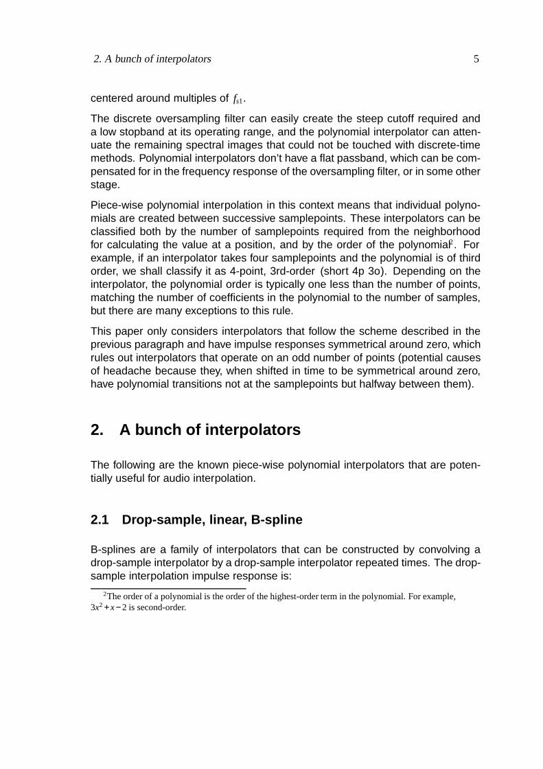
f (x) =
{1 0 ≤ x < 10 otherwise.
Formula, figure: Drop-sample interpolation (also the 0th-order B-spline)impulse response . The zero-amplitude areas are unmarked
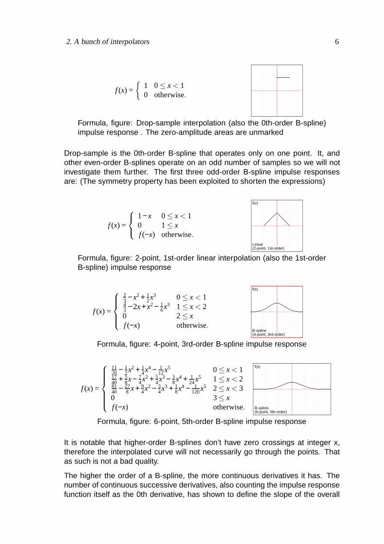
Drop-sample is the 0th-order B-spline that operates only on one point. It, andother even-order B-splines operate on an odd number of samples so we will notinvestigate them further. The first three odd-order B-spline impulse responsesare: (The symmetry property has been exploited to shorten the expressions)
f (x) =
1 −x 0 ≤ x < 10 1 ≤ xf (−x) otherwise.
f(x)f(x)
LinearLinear(2-point, 1st-order)(2-point, 1st-order)
Formula, figure: 2-point, 1st-order linear interpolation (also the 1st-orderB-spline) impulse response
f (x) =
23 −x2 + 1
2x3 0 ≤ x < 143 −2x +x2 − 1
6x3 1 ≤ x < 20 2 ≤ xf (−x) otherwise.
f(x)f(x)
B-splineB-spline(4-point, 3rd-order)(4-point, 3rd-order)
Formula, figure: 4-point, 3rd-order B-spline impulse response
f (x) =
1120 − 1
2x2 + 14x4 − 1
12 x5 0 ≤ x < 11740 + 5
8x − 74x2 + 5
4x3 − 38 x4 + 1
24x5 1 ≤ x < 28140 − 27
8 x + 94x2 − 3
4x3 + 18x4 − 1
120x5 2 ≤ x < 30 3 ≤ xf (−x) otherwise.
f(x)f(x)
B-splineB-spline(6-point, 5th-order)(6-point, 5th-order)
Formula, figure: 6-point, 5th-order B-spline impulse response
It is notable that higher-order B-splines don’t have zero crossings at integer x,therefore the interpolated curve will not necessarily go through the points. Thatas such is not a bad quality.
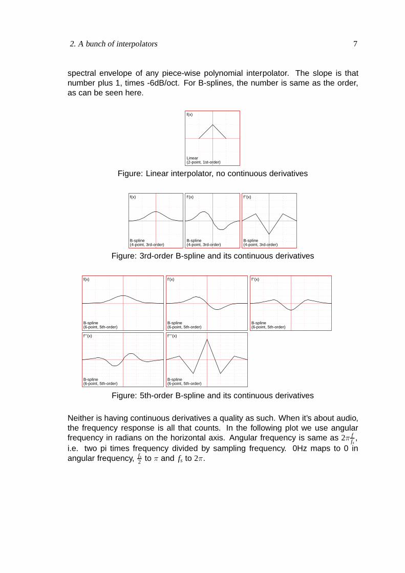
The higher the order of a B-spline, the more continuous derivatives it has. Thenumber of continuous successive derivatives, also counting the impulse responsefunction itself as the 0th derivative, has shown to define the slope of the overall
2. A bunch of interpolators 7
spectral envelope of any piece-wise polynomial interpolator. The slope is thatnumber plus 1, times -6dB/oct. For B-splines, the number is same as the order,as can be seen here.
f(x)f(x)
LinearLinear(2-point, 1st-order)(2-point, 1st-order)
Figure: Linear interpolator, no continuous derivatives
f(x)f(x)
B-splineB-spline(4-point, 3rd-order)(4-point, 3rd-order)
f’(x)f’(x)
B-splineB-spline(4-point, 3rd-order)(4-point, 3rd-order)
f’’(x)f’’(x)
B-splineB-spline(4-point, 3rd-order)(4-point, 3rd-order)
Figure: 3rd-order B-spline and its continuous derivatives
f(x)f(x)
B-splineB-spline(6-point, 5th-order)(6-point, 5th-order)
f’(x)f’(x)
B-splineB-spline(6-point, 5th-order)(6-point, 5th-order)
f’’(x)f’’(x)
B-splineB-spline(6-point, 5th-order)(6-point, 5th-order)
f’’’(x)f’’’(x)
B-splineB-spline(6-point, 5th-order)(6-point, 5th-order)
f’’’’(x)f’’’’(x)
B-splineB-spline(6-point, 5th-order)(6-point, 5th-order)
Figure: 5th-order B-spline and its continuous derivatives
Neither is having continuous derivatives a quality as such. When it’s about audio,the frequency response is all that counts. In the following plot we use angularfrequency in radians on the horizontal axis. Angular frequency is same as 2π f
fs,
i.e. two pi times frequency divided by sampling frequency. 0Hz maps to 0 inangular frequency, fs
2 to π and fs to 2π.

2. A bunch of interpolators 8
-144-144
-132-132
-120-120
-108-108
-96-96
-84-84
-72-72
-60-60
-48-48
-36-36
-24-24
-12-12
00
1212
00 11 22 33 44 55 66 77 88 99 1010 1111 1212 1313 1414 1515 1616
Mag
nitu
de (
dB)
Mag
nitu
de (
dB)
Angular frequency (pi)Angular frequency (pi)
Linear (2-point, 1st-order)Linear (2-point, 1st-order)
B-spline (4-point, 3rd-order)B-spline (4-point, 3rd-order)
B-spline (6-point, 5th-order)B-spline (6-point, 5th-order)
Figure: Frequency responses of the first three odd-order B-splines, in-cluding the linear interpolator
The frequency responses show wide holes at multiples of 2π. This means that asthe images of the lowest audio frequencies land on these areas, they get heavilyattenuated. On the other hand, the attenuation is not very strong at the images ofnear π frequencies. Also, with no oversampling, the highest audio frequencies inthe passpand are strongly attenuated, which certainly needs to be compensatedfor if higher-order B-splines are used with no oversampling. Typically, one wouldcalculate the quality of an interpolator as the signal-to-noise ratio directly from thefrequency response, for example by subtracting the magnitude at the strongestsidelobe top from the the magnitude at w = 0, but we will later show why this is notan adequate quality measure when the interpolated signal is sampled audio.
2.2 Lagrange
Lagrange polynomials are forced to go through a number of points. For exam-ple, the 4-point Lagrange interpolator polynomial is formed so that it goes throughall of the four neighboring points, and the middle section is used. The 1st-order(2-point) Lagrange interpolator is the linear interpolator, which was already pre-sented as part of the B-spline family. The order of the Lagrange polynomials isalways one less than the number of points. The third- and fifth-order Lagrangeimpulse responses are:
f (x) =
1 − 12x −x2 + 1
2x3 0 ≤ x < 11 − 11
6 x +x2 − 16 x3 1 ≤ x < 2
0 2 ≤ xf (−x) otherwise.
f(x)f(x)
LagrangeLagrange(4-point, 3rd-order)(4-point, 3rd-order)
Formula, figure: 4-point, 3rd-order Lagrange impulse response
2. A bunch of interpolators 9
f (x) =
1 − 13x − 5
4x2 + 512x3 + 1
4x4 − 112x5 0 ≤ x < 1
1 − 1312 x − 5
8x2 + 2524x3 − 3
8x4 + 124x5 1 ≤ x < 2
1 − 13760 x + 15
8 x2 − 1724 x3 + 1
8x4 − 1120x5 2 ≤ x < 3
0 3 ≤ xf (−x) otherwise.
f(x)f(x)
LagrangeLagrange(6-point, 5th-order)(6-point, 5th-order)
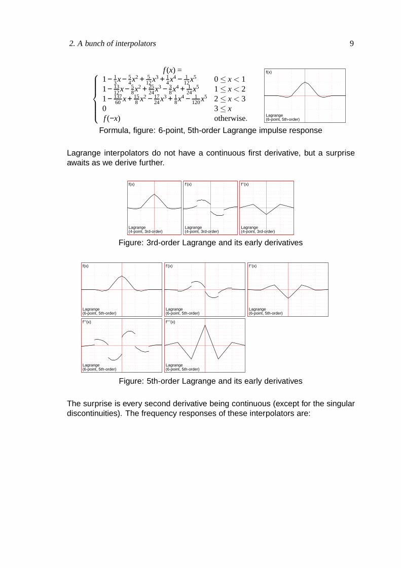
Formula, figure: 6-point, 5th-order Lagrange impulse response
Lagrange interpolators do not have a continuous first derivative, but a surpriseawaits as we derive further.
f(x)f(x)
LagrangeLagrange(4-point, 3rd-order)(4-point, 3rd-order)
f’(x)f’(x)
LagrangeLagrange(4-point, 3rd-order)(4-point, 3rd-order)
f’’(x)f’’(x)
LagrangeLagrange(4-point, 3rd-order)(4-point, 3rd-order)
Figure: 3rd-order Lagrange and its early derivatives
f(x)f(x)
LagrangeLagrange(6-point, 5th-order)(6-point, 5th-order)
f’(x)f’(x)
LagrangeLagrange(6-point, 5th-order)(6-point, 5th-order)
f’’(x)f’’(x)
LagrangeLagrange(6-point, 5th-order)(6-point, 5th-order)
f’’’(x)f’’’(x)
LagrangeLagrange(6-point, 5th-order)(6-point, 5th-order)
f’’’’(x)f’’’’(x)
LagrangeLagrange(6-point, 5th-order)(6-point, 5th-order)
Figure: 5th-order Lagrange and its early derivatives
The surprise is every second derivative being continuous (except for the singulardiscontinuities). The frequency responses of these interpolators are:
2. A bunch of interpolators 10
-144-144
-132-132
-120-120
-108-108
-96-96
-84-84
-72-72
-60-60
-48-48
-36-36
-24-24
-12-12
00
1212
00 11 22 33 44 55 66 77 88 99 1010 1111 1212 1313 1414 1515 1616
Mag
nitu
de (
dB)
Mag
nitu
de (
dB)
Angular frequency (pi)Angular frequency (pi)
Linear (2-point, 1st-order)Linear (2-point, 1st-order)
Lagrange (4-point, 3rd-order)Lagrange (4-point, 3rd-order)
Lagrange (6-point, 5th-order)Lagrange (6-point, 5th-order)
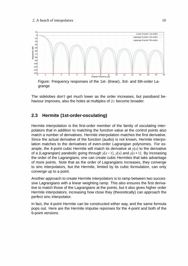
Figure: Frequency responses of the 1st- (linear), 3rd- and 5th-order La-grange
The sidelobes don’t get much lower as the order increases, but passband be-haviour improves, also the holes at multiples of 2π become broader.
2.3 Hermite (1st-order-osculating)
Hermite interpolation is the first-order member of the family of osculating inter-polators that in addition to matching the function value at the control points alsomatch a number of derivatives. Hermite interpolation matches the first derivative.Since the actual derivative of the function (audio) is not known, Hermite interpo-lation matches to the derivatives of even-order Lagrangian polynomes. For ex-ample, the 4-point cubic Hermite will match its derivative at y[x] to the derivativeof a (Lagrangian) parabolic going through y[x −1], y[x] and y[x +1]. By increasingthe order of the Lagrangians, one can create cubic Hermites that take advantageof more points. Note that as the order of Lagrangians increases, they convergeto sinc interpolators, but the Hermite, limited by its cubic formulation, can onlyconverge up to a point.
Another approach to create Hermite interpolators is to ramp between two succes-sive Lagrangians with a linear weighting ramp. This also ensures the first deriva-tive to match those of the Lagrangians at the points, but it also gives higher orderHermite interpolators, increasing how close they (theoretically) can approach theperfect sinc interpolator.
In fact, the 4-point Hermite can be constructed either way, and the same formulapops out. Here are the Hermite impulse reponses for the 4-point and both of the6-point versions.

2. A bunch of interpolators 11
f (x) =
1 − 52x2 + 3
2x3 0 ≤ x < 12 −4x + 5
2x2 − 12x3 1 ≤ x < 2
0 2 ≤ xf (−x) otherwise.
f(x)f(x)
HermiteHermite(4-point, 3rd-order)(4-point, 3rd-order)
Formula, figure: 4-point, 3rd-order Hermite impulse response. This isalso known as the Catmull-Rom spline, or the α = −1
2 case of cardinalsplines, where α is the derivative of the impulse response at x = 1.
f (x) =
1 − 73x2 + 4
3x3 0 ≤ x < 152 − 59
12x +3x2 − 712x3 1 ≤ x < 2
−32 + 7
4x − 23x2 + 1
12x3 2 ≤ x < 30 3 ≤ xf (−x) otherwise.
f(x)f(x)
HermiteHermite(6-point, 3rd-order)(6-point, 3rd-order)
Formula, figure: 6-point, 3rd-order Hermite impulse response(first derivative matches with the first derivatives of the Lagrangians)
f (x) =
1 − 2512 x2 + 5
12x3 + 1312 x4 − 5
12x5 0 ≤ x < 11 + 5
12 x − 358 x2 + 35
8 x3 − 138 x4 + 5
24 x5 1 ≤ x < 23 − 29
4 x + 15524 x2 − 65
24 x3 + 1324x4 − 1
24x5 2 ≤ x < 30 3 ≤ xf (−x) otherwise.
f(x)f(x)
HermiteHermite(6-point, 5th-order)(6-point, 5th-order)
Formula, figure: 6-point, 5th-order Hermite impulse response(linear ramp between two Lagrangians)
Hermite interpolators have a continuous first derivative by definition, but let’s takea deeper look anyhow.
f(x)f(x)
HermiteHermite(4-point, 3rd-order)(4-point, 3rd-order)
f’(x)f’(x)
HermiteHermite(4-point, 3rd-order)(4-point, 3rd-order)
f’’(x)f’’(x)
HermiteHermite(4-point, 3rd-order)(4-point, 3rd-order)
Figure: 4-point, 3rd-order Hermite and its early derivatives
f(x)f(x)
HermiteHermite(6-point, 3rd-order)(6-point, 3rd-order)
f’(x)f’(x)
HermiteHermite(6-point, 3rd-order)(6-point, 3rd-order)
f’’(x)f’’(x)
HermiteHermite(6-point, 3rd-order)(6-point, 3rd-order)
Figure: 6-point, 3rd-order Hermite nad its early derivatives
2. A bunch of interpolators 12
f(x)f(x)
HermiteHermite(6-point, 5th-order)(6-point, 5th-order)
f’(x)f’(x)
HermiteHermite(6-point, 5th-order)(6-point, 5th-order)
f’’(x)f’’(x)
HermiteHermite(6-point, 5th-order)(6-point, 5th-order)
f’’’(x)f’’’(x)
HermiteHermite(6-point, 5th-order)(6-point, 5th-order)
f’’’’(x)f’’’’(x)
HermiteHermite(6-point, 5th-order)(6-point, 5th-order)
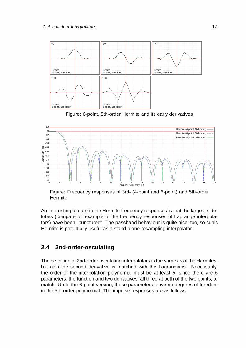
Figure: 6-point, 5th-order Hermite and its early derivatives
-144-144
-132-132
-120-120
-108-108
-96-96
-84-84
-72-72
-60-60
-48-48
-36-36
-24-24
-12-12
00
1212
00 11 22 33 44 55 66 77 88 99 1010 1111 1212 1313 1414 1515 1616
Mag
nitu
de (
dB)
Mag
nitu
de (
dB)
Angular frequency (pi)Angular frequency (pi)
Hermite (4-point, 3rd-order)Hermite (4-point, 3rd-order)
Hermite (6-point, 3rd-order)Hermite (6-point, 3rd-order)
Hermite (6-point, 5th-order)Hermite (6-point, 5th-order)
Figure: Frequency responses of 3rd- (4-point and 6-point) and 5th-orderHermite
An interesting feature in the Hermite frequency responses is that the largest side-lobes (compare for example to the frequency responses of Lagrange interpola-tors) have been "punctured". The passband behaviour is quite nice, too, so cubicHermite is potentially useful as a stand-alone resampling interpolator.
2.4 2nd-order-osculating
The definition of 2nd-order osculating interpolators is the same as of the Hermites,but also the second derivative is matched with the Lagrangians. Necessarily,the order of the interpolation polynomial must be at least 5, since there are 6parameters, the function and two derivatives, all three at both of the two points, tomatch. Up to the 6-point version, these parameters leave no degrees of freedomin the 5th-order polynomial. The impulse responses are as follows.
2. A bunch of interpolators 13
f (x) =
1 −x2 − 92x3 + 15
2 x4 −3x5 0 ≤ x < 1−4 +18x −29x2 + 43
2 x3 − 152 x4 +x5 1 ≤ x < 2
0 2 ≤ xf (−x) otherwise.
f(x)f(x)
2nd-order-osculating2nd-order-osculating(4-point, 5th-order)(4-point, 5th-order)
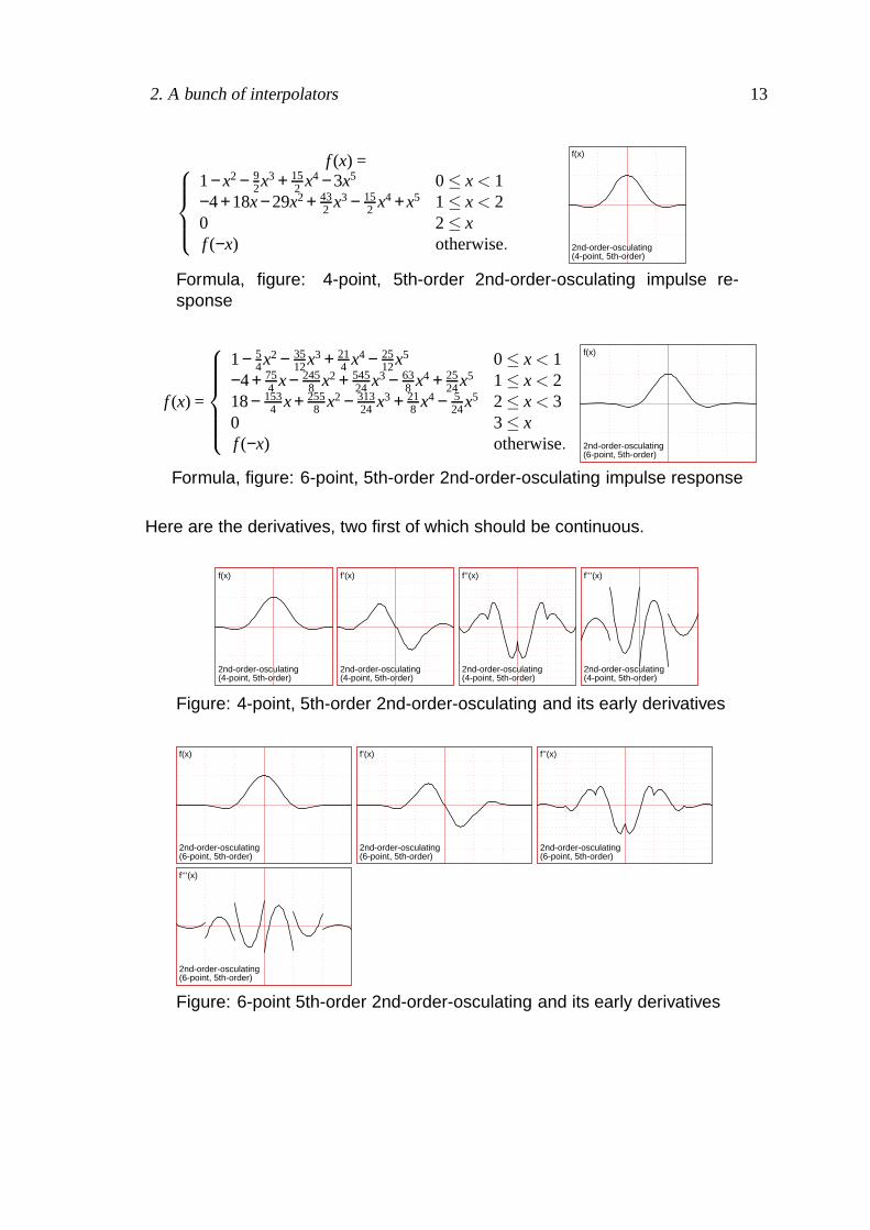
Formula, figure: 4-point, 5th-order 2nd-order-osculating impulse re-sponse
f (x) =
1 − 54x2 − 35
12x3 + 214 x4 − 25
12x5 0 ≤ x < 1−4 + 75
4 x − 2458 x2 + 545
24 x3 − 638 x4 + 25
24 x5 1 ≤ x < 218 − 153
4 x + 2558 x2 − 313
24 x3 + 218 x4 − 5
24x5 2 ≤ x < 30 3 ≤ xf (−x) otherwise.
f(x)f(x)
2nd-order-osculating2nd-order-osculating(6-point, 5th-order)(6-point, 5th-order)
Formula, figure: 6-point, 5th-order 2nd-order-osculating impulse response
Here are the derivatives, two first of which should be continuous.
f(x)f(x)
2nd-order-osculating2nd-order-osculating(4-point, 5th-order)(4-point, 5th-order)
f’(x)f’(x)
2nd-order-osculating2nd-order-osculating(4-point, 5th-order)(4-point, 5th-order)
f’’(x)f’’(x)
2nd-order-osculating2nd-order-osculating(4-point, 5th-order)(4-point, 5th-order)
f’’’(x)f’’’(x)
2nd-order-osculating2nd-order-osculating(4-point, 5th-order)(4-point, 5th-order)
Figure: 4-point, 5th-order 2nd-order-osculating and its early derivatives
f(x)f(x)
2nd-order-osculating2nd-order-osculating(6-point, 5th-order)(6-point, 5th-order)
f’(x)f’(x)
2nd-order-osculating2nd-order-osculating(6-point, 5th-order)(6-point, 5th-order)
f’’(x)f’’(x)
2nd-order-osculating2nd-order-osculating(6-point, 5th-order)(6-point, 5th-order)
f’’’(x)f’’’(x)
2nd-order-osculating2nd-order-osculating(6-point, 5th-order)(6-point, 5th-order)
Figure: 6-point 5th-order 2nd-order-osculating and its early derivatives
2. A bunch of interpolators 14
-144-144
-132-132
-120-120
-108-108
-96-96
-84-84
-72-72
-60-60
-48-48
-36-36
-24-24
-12-12
00
1212
00 11 22 33 44 55 66 77 88 99 1010 1111 1212 1313 1414 1515 1616
Mag
nitu
de (
dB)
Mag
nitu
de (
dB)
Angular frequency (pi)Angular frequency (pi)
2nd-order-osculating (4-point, 5th-order)2nd-order-osculating (4-point, 5th-order)
2nd-order-osculating (6-point, 5th-order)2nd-order-osculating (6-point, 5th-order)
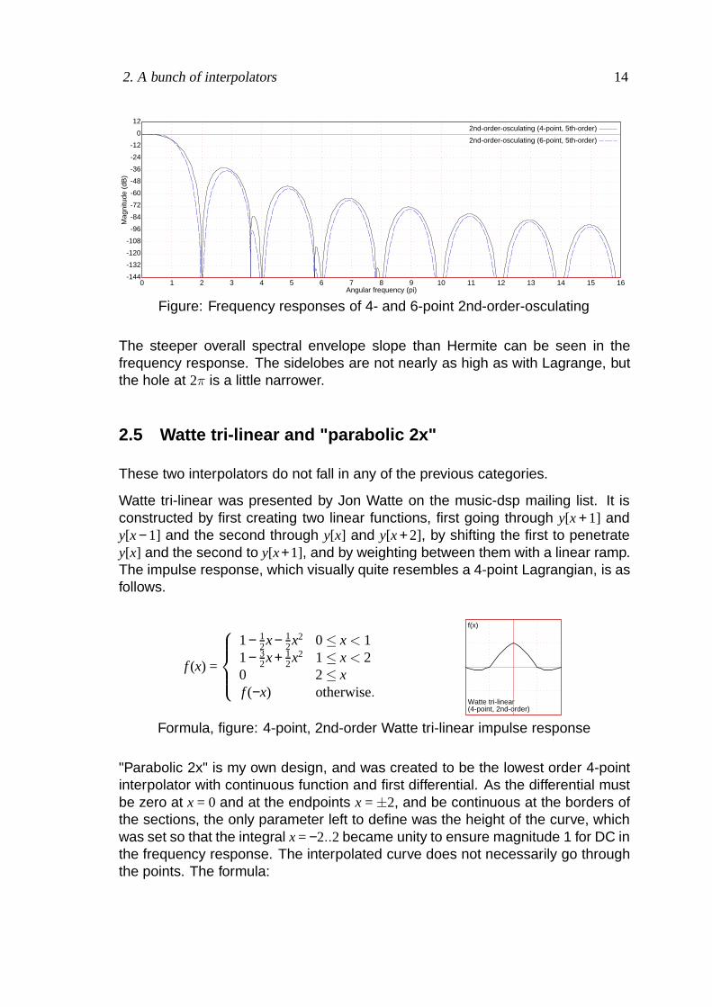
Figure: Frequency responses of 4- and 6-point 2nd-order-osculating
The steeper overall spectral envelope slope than Hermite can be seen in thefrequency response. The sidelobes are not nearly as high as with Lagrange, butthe hole at 2π is a little narrower.
2.5 Watte tri-linear and "parabolic 2x"
These two interpolators do not fall in any of the previous categories.
Watte tri-linear was presented by Jon Watte on the music-dsp mailing list. It isconstructed by first creating two linear functions, first going through y[x +1] andy[x −1] and the second through y[x] and y[x +2], by shifting the first to penetratey[x] and the second to y[x+1], and by weighting between them with a linear ramp.The impulse response, which visually quite resembles a 4-point Lagrangian, is asfollows.
f (x) =
1 − 12x − 1
2x2 0 ≤ x < 11 − 3
2x + 12x2 1 ≤ x < 2
0 2 ≤ xf (−x) otherwise.
f(x)f(x)
Watte tri-linearWatte tri-linear(4-point, 2nd-order)(4-point, 2nd-order)
Formula, figure: 4-point, 2nd-order Watte tri-linear impulse response
"Parabolic 2x" is my own design, and was created to be the lowest order 4-pointinterpolator with continuous function and first differential. As the differential mustbe zero at x = 0 and at the endpoints x = ±2, and be continuous at the borders ofthe sections, the only parameter left to define was the height of the curve, whichwas set so that the integral x = −2..2 became unity to ensure magnitude 1 for DC inthe frequency response. The interpolated curve does not necessarily go throughthe points. The formula:

2. A bunch of interpolators 15
f (x) =
12 − 1
4 x2 0 ≤ x < 11 −x + 1
4x2 1 ≤ x < 20 2 ≤ xf (−x) otherwise.
f(x)f(x)
Parabolic 2xParabolic 2x(4-point, 2nd-order)(4-point, 2nd-order)
Formula, figure: 4-point, 2nd-order parabolic 2x impulse response
Just for the fun of it, the derivatives for these odd-balls, followed by the frequencyresponse plots:
f(x)f(x)
Watte tri-linearWatte tri-linear(4-point, 2nd-order)(4-point, 2nd-order)
f’(x)f’(x)
Watte tri-linearWatte tri-linear(4-point, 2nd-order)(4-point, 2nd-order)
f’’(x)f’’(x)
Watte tri-linearWatte tri-linear(4-point, 2nd-order)(4-point, 2nd-order)
Figure: Watte tri-linear and its early derivatives
f(x)f(x)
Parabolic 2xParabolic 2x(4-point, 2nd-order)(4-point, 2nd-order)
f’(x)f’(x)
Parabolic 2xParabolic 2x(4-point, 2nd-order)(4-point, 2nd-order)
f’’(x)f’’(x)
Parabolic 2xParabolic 2x(4-point, 2nd-order)(4-point, 2nd-order)
Figure: Parabolic 2x and its early derivatives
-144-144
-132-132
-120-120
-108-108
-96-96
-84-84
-72-72
-60-60
-48-48
-36-36
-24-24
-12-12
00
1212
00 11 22 33 44 55 66 77 88 99 1010 1111 1212 1313 1414 1515 1616
Mag
nitu
de (
dB)
Mag
nitu
de (
dB)
Angular frequency (pi)Angular frequency (pi)
Watte tri-linear (4-point, 2nd-order)Watte tri-linear (4-point, 2nd-order)
Parabolic 2x (4-point, 2nd-order)Parabolic 2x (4-point, 2nd-order)
Figure: Frequency responses of Watte tri-linear and parabolic 2x
Looking at the frequency responses (put in the same graph to save paper), Wattetri-linear has an extraordinary steep cutoff slope, until the first short sidelobe.Parabolic 2x has a hole at π, which makes it suitable for use with oversampleddata only. It has nicely low sidelobes and wide holes at multiples of 2π though.
3. A quality measure 16
3. A quality measure
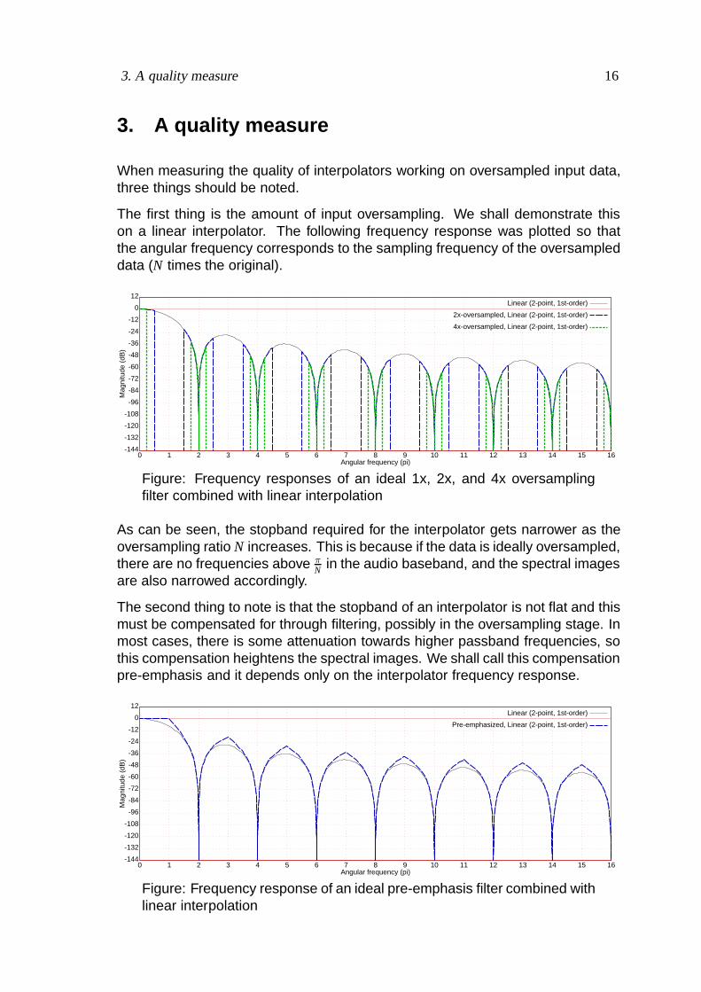
When measuring the quality of interpolators working on oversampled input data,three things should be noted.
The first thing is the amount of input oversampling. We shall demonstrate thison a linear interpolator. The following frequency response was plotted so thatthe angular frequency corresponds to the sampling frequency of the oversampleddata (N times the original).
-144-144
-132-132
-120-120
-108-108
-96-96
-84-84
-72-72
-60-60
-48-48
-36-36
-24-24
-12-12
00
1212
00 11 22 33 44 55 66 77 88 99 1010 1111 1212 1313 1414 1515 1616
Mag
nitu
de (
dB)
Mag
nitu
de (
dB)
Angular frequency (pi)Angular frequency (pi)
Linear (2-point, 1st-order)Linear (2-point, 1st-order)
2x-oversampled, Linear (2-point, 1st-order)2x-oversampled, Linear (2-point, 1st-order)
4x-oversampled, Linear (2-point, 1st-order)4x-oversampled, Linear (2-point, 1st-order)
Figure: Frequency responses of an ideal 1x, 2x, and 4x oversamplingfilter combined with linear interpolation
As can be seen, the stopband required for the interpolator gets narrower as theoversampling ratio N increases. This is because if the data is ideally oversampled,there are no frequencies above π
N in the audio baseband, and the spectral imagesare also narrowed accordingly.
The second thing to note is that the stopband of an interpolator is not flat and thismust be compensated for through filtering, possibly in the oversampling stage. Inmost cases, there is some attenuation towards higher passband frequencies, sothis compensation heightens the spectral images. We shall call this compensationpre-emphasis and it depends only on the interpolator frequency response.
-144-144
-132-132
-120-120
-108-108
-96-96
-84-84
-72-72
-60-60
-48-48
-36-36
-24-24
-12-12
00
1212
00 11 22 33 44 55 66 77 88 99 1010 1111 1212 1313 1414 1515 1616
Mag
nitu
de (
dB)
Mag
nitu
de (
dB)
Angular frequency (pi)Angular frequency (pi)
Linear (2-point, 1st-order)Linear (2-point, 1st-order)
Pre-emphasized, Linear (2-point, 1st-order)Pre-emphasized, Linear (2-point, 1st-order)
Figure: Frequency response of an ideal pre-emphasis filter combined withlinear interpolation

3. A quality measure 17
The third thing to note is that audio generally has a pink spectral envelope. Thisis a much better presumption than white. Pieces of music are generally equalizedto pink. Pink means that the spectrum decreases 3dB per an octave increasein frequency. To take this into account in interpolator quality evaluation, we filterthe spectral images with a pinking filter, whose magnitude is proportional to 1√
w ,where w is the angular frequency of the passband frequency that creates theimage. We shall call this process pinking. The pinking filter is normalized so thatthe magnitude at stopband edges is unity, so the pinking filter depends only onthe amount of oversampling. The frequency responses of the pinking filters are:
-12-12
00
1212
2424
3636
4848
6060
7272
8484
9696
108108
00 11 22 33 44 55 66 77 88 99 1010 1111 1212 1313 1414 1515 1616
Mag
nitu
de (
dB)
Mag
nitu
de (
dB)
Angular frequency (pi)Angular frequency (pi)
Pinking filter for unoversampledPinking filter for unoversampled
Pinking filter for 2x-oversampledPinking filter for 2x-oversampled
Pinking filter for 4x-oversampledPinking filter for 4x-oversampled
Pinking filter for 8x-oversampledPinking filter for 8x-oversampled
Pinking filter for 16x-oversampledPinking filter for 16x-oversampled
Pinking filter for 32x-oversampledPinking filter for 32x-oversampled
Figure: Frequency responses of the pinking filters
A demonstration on pinking:
-144-144
-132-132
-120-120
-108-108
-96-96
-84-84
-72-72
-60-60
-48-48
-36-36
-24-24
-12-12
00
1212
00 11 22 33 44 55 66 77 88 99 1010 1111 1212 1313 1414 1515 1616
Mag
nitu
de (
dB)
Mag
nitu
de (
dB)
Angular frequency (pi)Angular frequency (pi)
Linear (2-point, 1st-order)Linear (2-point, 1st-order)
Pinked, Linear (2-point, 1st-order)Pinked, Linear (2-point, 1st-order)
Figure: Normal and pinked frequency response of linear interpolation(with no oversampling)
In the demonstration with linear interpolation, pinking has a notable effect - thefirst sidelobe top has moved left and heightened sligtly.
Pinking emphasizes the importance of stopband attenuation near frequencies amultiple of 2π. This has proven to be important as some interpolators may haveOK-looking frequency responses, but sound really bad when there are typicalamounts of low frequencies in the input, compared to testing with white noise. Be-cause pinking would be infinitely strong near 0Hz, we choose to keep increasing
4. New optimal designs 18
the pinking gain only down to the frequency corresponding to 5Hz in a 44100Hzsampling frequency (before oversampling) input signal, and keep the pinking gainat the same level from that point to 0Hz.
The effects of the oversampling, pre-emphasis and pinking can be combined.We shall call the frequency responses obtained this way modified frequency re-sponses. From a modified frequency response, we shall find the maximum (peak)magnitude frequency response from the stopbands, convert that to dB, flip thesign, and call this value the modified SNR (signal-to-noise ratio) and presumethat it is a rather good and comparable measure of the quality of an interpolator.
Interpolating non-oversampled data is out of the scope of this kind of a compari-son. There would be problems with defining the passband-to-stopband transitionband. With the presumption of an ideal oversampling filter, the transition bands ofthe interpolator are rendered invisible. Also, the passband attenuation is not anissue because of pre-emphasis, which shows its price at the stopbands.
4. New optimal designs
With the modified SNR as a quality measure, it was possible to design the bestpossible interpolators of chosen oversampling ratios, orders and numbers of points.
The optimization was done directly on the impulse response coefficients, usingDifferential Evolution3, a genetic algorithm developed by Rainer Storn and Ken-neth Price. In short, the algorithm finds (or at least tries to) the global minimum ofa cost function that takes a parameter vector as an argument, which in this caseconsisted of the coefficients of the polynomial(s). In the cost function, the sixfirst stopbands in the modified frequency response were sampled at 33 positionseach, and the largest magnitude was given as the cost which was then minimizedby the Differential Evolution algorithm. The normalization for unity gain at DC wasalso implemented as an added penalty in the cost function.
Here are the impulse responses of all the potentially useful generated interpola-tors for oversampling ratios 2, 4, 8, 16 and 32. Note that there is some air in thedecimals of the coefficients, so some further quantization is OK.
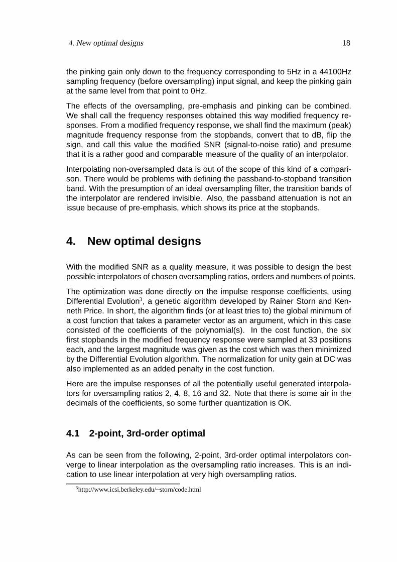
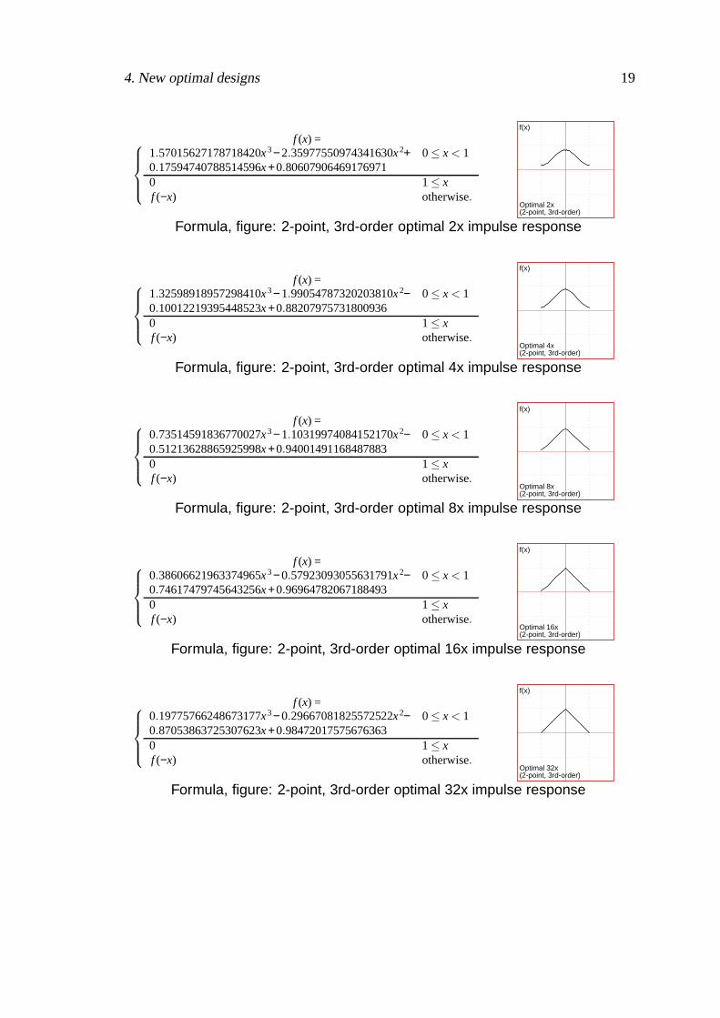
4.1 2-point, 3rd-order optimal
As can be seen from the following, 2-point, 3rd-order optimal interpolators con-verge to linear interpolation as the oversampling ratio increases. This is an indi-cation to use linear interpolation at very high oversampling ratios.
3http://www.icsi.berkeley.edu/~storn/code.html
4. New optimal designs 19
f (x) =
1.57015627178718420x 3 −2.35977550974341630x 2+ 0 ≤ x < 10.17594740788514596x +0.806079064691769710 1 ≤ xf (−x) otherwise.
f(x)f(x)
Optimal 2xOptimal 2x(2-point, 3rd-order)(2-point, 3rd-order)
Formula, figure: 2-point, 3rd-order optimal 2x impulse response
f (x) =
1.32598918957298410x 3 −1.99054787320203810x 2− 0 ≤ x < 10.10012219395448523x +0.882079757318009360 1 ≤ xf (−x) otherwise.
f(x)f(x)
Optimal 4xOptimal 4x(2-point, 3rd-order)(2-point, 3rd-order)
Formula, figure: 2-point, 3rd-order optimal 4x impulse response
f (x) =
0.73514591836770027x 3 −1.10319974084152170x 2− 0 ≤ x < 10.51213628865925998x +0.940014911684878830 1 ≤ xf (−x) otherwise.
f(x)f(x)
Optimal 8xOptimal 8x(2-point, 3rd-order)(2-point, 3rd-order)
Formula, figure: 2-point, 3rd-order optimal 8x impulse response
f (x) =
0.38606621963374965x 3 −0.57923093055631791x 2− 0 ≤ x < 10.74617479745643256x +0.969647820671884930 1 ≤ xf (−x) otherwise.
f(x)f(x)
Optimal 16xOptimal 16x(2-point, 3rd-order)(2-point, 3rd-order)
Formula, figure: 2-point, 3rd-order optimal 16x impulse response
f (x) =
0.19775766248673177x 3 −0.29667081825572522x 2− 0 ≤ x < 10.87053863725307623x +0.984720175756763630 1 ≤ xf (−x) otherwise.
f(x)f(x)
Optimal 32xOptimal 32x(2-point, 3rd-order)(2-point, 3rd-order)
Formula, figure: 2-point, 3rd-order optimal 32x impulse response

4. New optimal designs 20
-144-144-132-132-120-120-108-108-96-96-84-84-72-72-60-60-48-48-36-36-24-24-12-12
001212
00 11 22 33 44 55 66 77 88 99 1010 1111 1212 1313
Mag
nitu
de (
dB)
Mag
nitu
de (
dB)
Angular frequency (pi)Angular frequency (pi)
Optimal 2x (2-point, 3rd-order)Optimal 2x (2-point, 3rd-order)Optimal 4x (2-point, 3rd-order)Optimal 4x (2-point, 3rd-order)Optimal 8x (2-point, 3rd-order)Optimal 8x (2-point, 3rd-order)
Optimal 16x (2-point, 3rd-order)Optimal 16x (2-point, 3rd-order)Optimal 32x (2-point, 3rd-order)Optimal 32x (2-point, 3rd-order)
Figure: Frequency responses of 2-point, 3rd-order optimal interpolatorsfor different oversampling ratios
The modified frequency responses will be shown in the comparison section of thispaper.
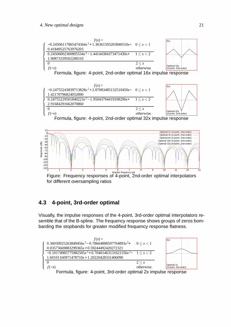
4.2 4-point, 2nd-order optimal
The 4-point, 2nd-order optimal interpolators are a bit strange - the impulse re-sponses, especially the higher oversampling ratio versions, do not even resembleanything that we have previously seen. The explanation is that there is a transferfunction zero on the transition band. This causes a large sidelobe that at higheroversampling ratios exceeds unity in magnitude.
f (x) =
−0.21343978756177684x 2−0.04782068534965925x+ 0 ≤ x < 10.500616622137526560.21303593243799016x 2 −0.88689658749623701x+ 1 ≤ x < 20.927701355280273860 2 ≤ xf (−x) otherwise.
f(x)f(x)
Optimal 2xOptimal 2x(4-point, 2nd-order)(4-point, 2nd-order)
Formula, figure: 4-point, 2nd-order optimal 2x impulse response
f (x) =
−0.22865399531858188x 2+0.21144498075197282x+ 0 ≤ x < 10.338203657365671150.22858390767180370x 2 −1.01414466618792900x+ 1 ≤ x < 21.120146398745554700 2 ≤ xf (−x) otherwise.
f(x)f(x)
Optimal 4xOptimal 4x(4-point, 2nd-order)(4-point, 2nd-order)
Formula, figure: 4-point, 2nd-order optimal 4x impulse response
f (x) =
−0.24005206207889518x 2+0.59257579283164508x+ 0 ≤ x < 10.092247185742041720.24004281672637814x 2 −1.17126532964206100x+ 1 ≤ x < 21.388280360636643200 2 ≤ xf (−x) otherwise.
f(x)f(x)
Optimal 8xOptimal 8x(4-point, 2nd-order)(4-point, 2nd-order)
Formula, figure: 4-point, 2nd-order optimal 8x impulse response
4. New optimal designs 21
f (x) =
−0.24506117865474364x 2+1.36361593203840510x− 0 ≤ x < 10.418495257639762030.24506002360805534x 2 −1.44144384373471430x+ 1 ≤ x < 21.908733395022083100 2 ≤ xf (−x) otherwise.
f(x)f(x)
Optimal 16xOptimal 16x(4-point, 2nd-order)(4-point, 2nd-order)
Formula, figure: 4-point, 2nd-order optimal 16x impulse response
f (x) =
−0.24755243839713828x 2+2.87083485132510450x− 0 ≤ x < 11.421707968240528900.24755229501840223x 2 −1.95043794419108290x+ 1 ≤ x < 22.916842916620708600 2 ≤ xf (−x) otherwise.
f(x)f(x)
Optimal 32xOptimal 32x(4-point, 2nd-order)(4-point, 2nd-order)
Formula, figure: 4-point, 2nd-order optimal 32x impulse response
-144-144-132-132-120-120-108-108-96-96-84-84-72-72-60-60-48-48-36-36-24-24-12-12
001212
00 11 22 33 44 55 66 77 88 99 1010 1111 1212 1313
Mag
nitu
de (
dB)
Mag
nitu
de (
dB)
Angular frequency (pi)Angular frequency (pi)
Optimal 2x (4-point, 2nd-order)Optimal 2x (4-point, 2nd-order)Optimal 4x (4-point, 2nd-order)Optimal 4x (4-point, 2nd-order)Optimal 8x (4-point, 2nd-order)Optimal 8x (4-point, 2nd-order)
Optimal 16x (4-point, 2nd-order)Optimal 16x (4-point, 2nd-order)Optimal 32x (4-point, 2nd-order)Optimal 32x (4-point, 2nd-order)
Figure: Frequency responses of 4-point, 2nd-order optimal interpolatorsfor different oversampling ratios
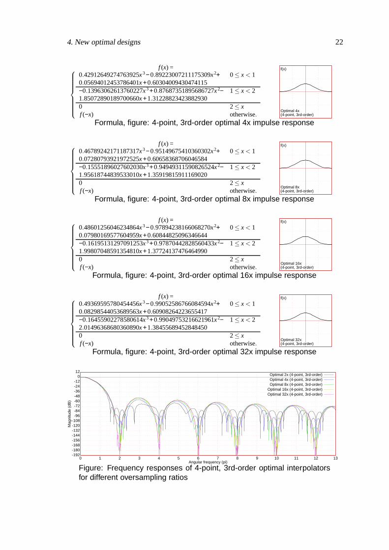
4.3 4-point, 3rd-order optimal
Visually, the impulse responses of the 4-point, 3rd-order optimal interpolators re-semble that of the B-spline. The frequency response shows groups of zeros bom-barding the stopbands for greater modified frequency response flatness.
f (x) =
0.36030925263849456x 3 −0.78664888597764893x2+ 0 ≤ x < 10.03573669883299365x +0.59244492420272321−0.10174985775982505x 3 +0.70401463131621556x 2− 1 ≤ x < 21.60101160971478710x +1.202204283314060900 2 ≤ xf (−x) otherwise.
f(x)f(x)
Optimal 2xOptimal 2x(4-point, 3rd-order)(4-point, 3rd-order)
Formula, figure: 4-point, 3rd-order optimal 2x impulse response
4. New optimal designs 22
f (x) =
0.42912649274763925x 3 −0.89223007211175309x2+ 0 ≤ x < 10.05694012453786401x +0.60304009430474115−0.13963062613760227x 3 +0.87687351895686727x 2− 1 ≤ x < 21.85072890189700660x +1.312288234238829300 2 ≤ xf (−x) otherwise.
f(x)f(x)
Optimal 4xOptimal 4x(4-point, 3rd-order)(4-point, 3rd-order)
Formula, figure: 4-point, 3rd-order optimal 4x impulse response
f (x) =
0.46789242171187317x 3 −0.95149675410360302x2+ 0 ≤ x < 10.07280793921972525x +0.60658368706046584−0.15551896027602030x 3 +0.94949311590826524x 2− 1 ≤ x < 21.95618744839533010x +1.359198159111690200 2 ≤ xf (−x) otherwise.
f(x)f(x)
Optimal 8xOptimal 8x(4-point, 3rd-order)(4-point, 3rd-order)
Formula, figure: 4-point, 3rd-order optimal 8x impulse response
f (x) =
0.48601256046234864x 3 −0.97894238166068270x2+ 0 ≤ x < 10.07980169577604959x +0.60844825096346644−0.16195131297091253x 3 +0.97870442828560433x 2− 1 ≤ x < 21.99807048591354810x +1.377241374764649900 2 ≤ xf (−x) otherwise.
f(x)f(x)
Optimal 16xOptimal 16x(4-point, 3rd-order)(4-point, 3rd-order)
Formula, figure: 4-point, 3rd-order optimal 16x impulse response
f (x) =
0.49369595780454456x 3 −0.99052586766084594x2+ 0 ≤ x < 10.08298544053689563x +0.60908264223655417−0.16455902278580614x 3 +0.99049753216621961x 2− 1 ≤ x < 22.01496368680360890x +1.384556894528484500 2 ≤ xf (−x) otherwise.
f(x)f(x)
Optimal 32xOptimal 32x(4-point, 3rd-order)(4-point, 3rd-order)
Formula, figure: 4-point, 3rd-order optimal 32x impulse response
-192-192-180-180-168-168-156-156-144-144-132-132-120-120-108-108-96-96-84-84-72-72-60-60-48-48-36-36-24-24-12-12
001212
00 11 22 33 44 55 66 77 88 99 1010 1111 1212 1313
Mag
nitu
de (
dB)
Mag
nitu
de (
dB)
Angular frequency (pi)Angular frequency (pi)
Optimal 2x (4-point, 3rd-order)Optimal 2x (4-point, 3rd-order)Optimal 4x (4-point, 3rd-order)Optimal 4x (4-point, 3rd-order)Optimal 8x (4-point, 3rd-order)Optimal 8x (4-point, 3rd-order)
Optimal 16x (4-point, 3rd-order)Optimal 16x (4-point, 3rd-order)Optimal 32x (4-point, 3rd-order)Optimal 32x (4-point, 3rd-order)
Figure: Frequency responses of 4-point, 3rd-order optimal interpolatorsfor different oversampling ratios
4. New optimal designs 23
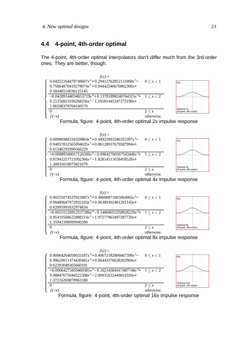
4.4 4-point, 4th-order optimal
The 4-point, 4th-order optimal interpolators don’t differ much from the 3rd-orderones. They are better, though.
f (x) =
0.04252164479749607x 4 +0.29412762852131868x3− 0 ≤ x < 10.75864870418278074x 2 +0.04442540676862300x+0.58448510036125145−0.04289144034653719x 4 +0.13781898240764315x 3+ 1 ≤ x < 20.21256821036268256x 2 −1.16581445347275190x+1.065983797041605700 2 ≤ xf (−x) otherwise.
f(x)f(x)
Optimal 2xOptimal 2x(4-point, 4th-order)(4-point, 4th-order)
Formula, figure: 4-point, 4th-order optimal 2x impulse response
f (x) =
0.00986988334359864x 4 +0.44922093286355397x3− 0 ≤ x < 10.94057832565094635x 2 +0.06128937679587994x+0.61340295990566229−0.00989340017126506x 4 −0.09642760567543440x 3+ 1 ≤ x < 20.81943257721092366x 2 −1.82814511658458520x+1.308350180758216700 2 ≤ xf (−x) otherwise.
f(x)f(x)
Optimal 4xOptimal 4x(4-point, 4th-order)(4-point, 4th-order)
Formula, figure: 4-point, 4th-order optimal 4x impulse response
f (x) =
0.00255074537015887x 4 +0.48698871865064902x3− 0 ≤ x < 10.98489647972932193x 2 +0.06389302461261143x+0.62095991632974834−0.00255226912537286x 4 −0.14868053358928229x 3+ 1 ≤ x < 20.95410568622888214x 2 −1.97277963497287720x+1.359433989999403900 2 ≤ xf (−x) otherwise.
f(x)f(x)
Optimal 8xOptimal 8x(4-point, 4th-order)(4-point, 4th-order)
Formula, figure: 4-point, 4th-order optimal 8x impulse response
f (x) =
0.00064264050033187x 4 +0.49672182806667398x3− 0 ≤ x < 10.99620011474430481x 2 +0.06443376638262904x+0.62293049365660191−0.00064273459469381x 4 −0.16214364417487748x 3+ 1 ≤ x < 20.98847675044522398x 2 −2.00931632449031920x+1.372162698789631800 2 ≤ xf (−x) otherwise.
f(x)f(x)
Optimal 16xOptimal 16x(4-point, 4th-order)(4-point, 4th-order)
Formula, figure: 4-point, 4th-order optimal 16x impulse response
4. New optimal designs 24
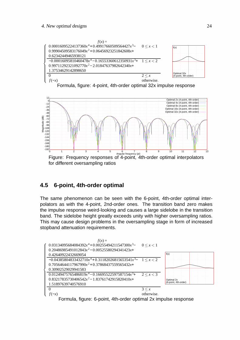
f (x) =
0.00016095224137360x 4 +0.49917660509564427x3− 0 ≤ x < 10.99904509583176049x 2 +0.06456923251842608x+0.62342449465938121−0.00016095810460478x 4 −0.16553360612350931x 3+ 1 ≤ x < 20.99711292321092770x 2 −2.01847637982642340x+1.375346291428986500 2 ≤ xf (−x) otherwise.
f(x)f(x)
Optimal 32xOptimal 32x(4-point, 4th-order)(4-point, 4th-order)
Formula, figure: 4-point, 4th-order optimal 32x impulse response
-192-192-180-180-168-168-156-156-144-144-132-132-120-120-108-108-96-96-84-84-72-72-60-60-48-48-36-36-24-24-12-12
001212
00 11 22 33 44 55 66 77 88 99 1010 1111 1212 1313
Mag
nitu
de (
dB)
Mag
nitu
de (
dB)
Angular frequency (pi)Angular frequency (pi)
Optimal 2x (4-point, 4th-order)Optimal 2x (4-point, 4th-order)Optimal 4x (4-point, 4th-order)Optimal 4x (4-point, 4th-order)Optimal 8x (4-point, 4th-order)Optimal 8x (4-point, 4th-order)
Optimal 16x (4-point, 4th-order)Optimal 16x (4-point, 4th-order)Optimal 32x (4-point, 4th-order)Optimal 32x (4-point, 4th-order)
Figure: Frequency responses of 4-point, 4th-order optimal interpolatorsfor different oversampling ratios
4.5 6-point, 4th-order optimal
The same phenomenon can be seen with the 6-point, 4th-order optimal inter-polators as with the 4-point, 2nd-order ones. The transition band zero makesthe impulse response weird-looking and causes a large sidelobe in the transitionband. The sidelobe height greatly exceeds unity with higher oversampling ratios.This may cause design problems in the oversampling stage in form of increasedstopband attenuation requirements.
f (x) =
0.03134095684084392x 4 +0.00255494211547300x3− 0 ≤ x < 10.20486985491012843x 2 −0.00525580294341423x+0.42640922432669054−0.04385804833432710x 4 +0.31182026815653541x 3− 1 ≤ x < 20.70564644117967990x 2 +0.37868437559565432x+0.309025290299415830.01249475765486819x 4 −0.16695522597587154x3+ 2 ≤ x < 30.83217835730406542x 2 −1.83761742915820410x+1.518976397405769100 3 ≤ xf (−x) otherwise.
f(x)f(x)
Optimal 2xOptimal 2x(6-point, 4th-order)(6-point, 4th-order)
Formula, figure: 6-point, 4th-order optimal 2x impulse response
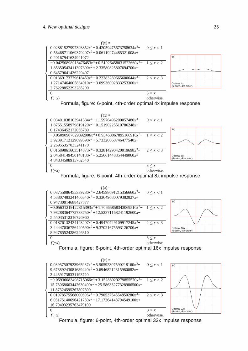
4. New optimal designs 25
f (x) =
0.02881527997393852x 4 −0.42059475673758634x3+ 0 ≤ x < 10.56468711069379207x 2 −0.06119274485321008x+0.20167941634921072−0.04250898918476453x 4 +0.51926458031522660x 3− 1 ≤ x < 21.85350543411307390x 2 +2.33580825807694700x−0.645796414362294070.01369173779618459x 4 −0.22283280665600644x3+ 2 ≤ x < 31.27147464005834010x 2 −3.09936092833253300x+2.762288522932852000 3 ≤ xf (−x) otherwise.
f(x)f(x)
Optimal 4xOptimal 4x(6-point, 4th-order)(6-point, 4th-order)
Formula, figure: 6-point, 4th-order optimal 4x impulse response
f (x) =
0.03401038103941584x 4 −1.15976496200057480x3+ 0 ≤ x < 11.87551558979819120x 2 −0.15190225510786248x−0.17436452172055789−0.05090907029392906x 4 +0.93463067895166918x 3− 1 ≤ x < 23.92391712129699590x 2 +5.73320660746477540x−2.269553570352411700.01689861603514873x 4 −0.32814290420019698x3+ 2 ≤ x < 32.04584149450148180x 2 −5.25661448354449060x+4.848345089157625400 3 ≤ xf (−x) otherwise.
f(x)f(x)
Optimal 8xOptimal 8x(6-point, 4th-order)(6-point, 4th-order)
Formula, figure: 6-point, 4th-order optimal 8x impulse response
f (x) =
0.03755086455339280x 4 −2.64598691215356660x3+ 0 ≤ x < 14.53807483241466340x 2 −0.33649680079382827x−0.94730014688427577−0.05631219122315393x 4 +1.70665858343069510x 3− 1 ≤ x < 27.98288364772738750x 2 +12.52871168241192600x−5.550353123167269600.01876132424143207x 4 −0.49470749109917245x3+ 2 ≤ x < 33.44447036756440590x 2 −9.37021675593126700x+8.947855242862463100 3 ≤ xf (−x) otherwise.
f(x)f(x)
Optimal 16xOptimal 16x(6-point, 4th-order)(6-point, 4th-order)
Formula, figure: 6-point, 4th-order optimal 16x impulse response
f (x) =
0.03957507923965987x 4 −5.50592307590218160x 3+ 0 ≤ x < 19.67889243081689440x 2 −0.69468212315980082x−2.44391738331193720−0.05936083498715066x 4 +3.15288929279855570x 3− 1 ≤ x < 215.73068663442630400x 2 +25.58633277328986500x−11.875245952678076000.01978575568000696x 4 −0.79053754554850286x 3+ 2 ≤ x < 36.05175140696421730x 2 −17.17264148794549100x+16.794032357634791000 3 ≤ xf (−x) otherwise.
f(x)f(x)
Optimal 32xOptimal 32x(6-point, 4th-order)(6-point, 4th-order)
Formula, figure: 6-point, 4th-order optimal 32x impulse response
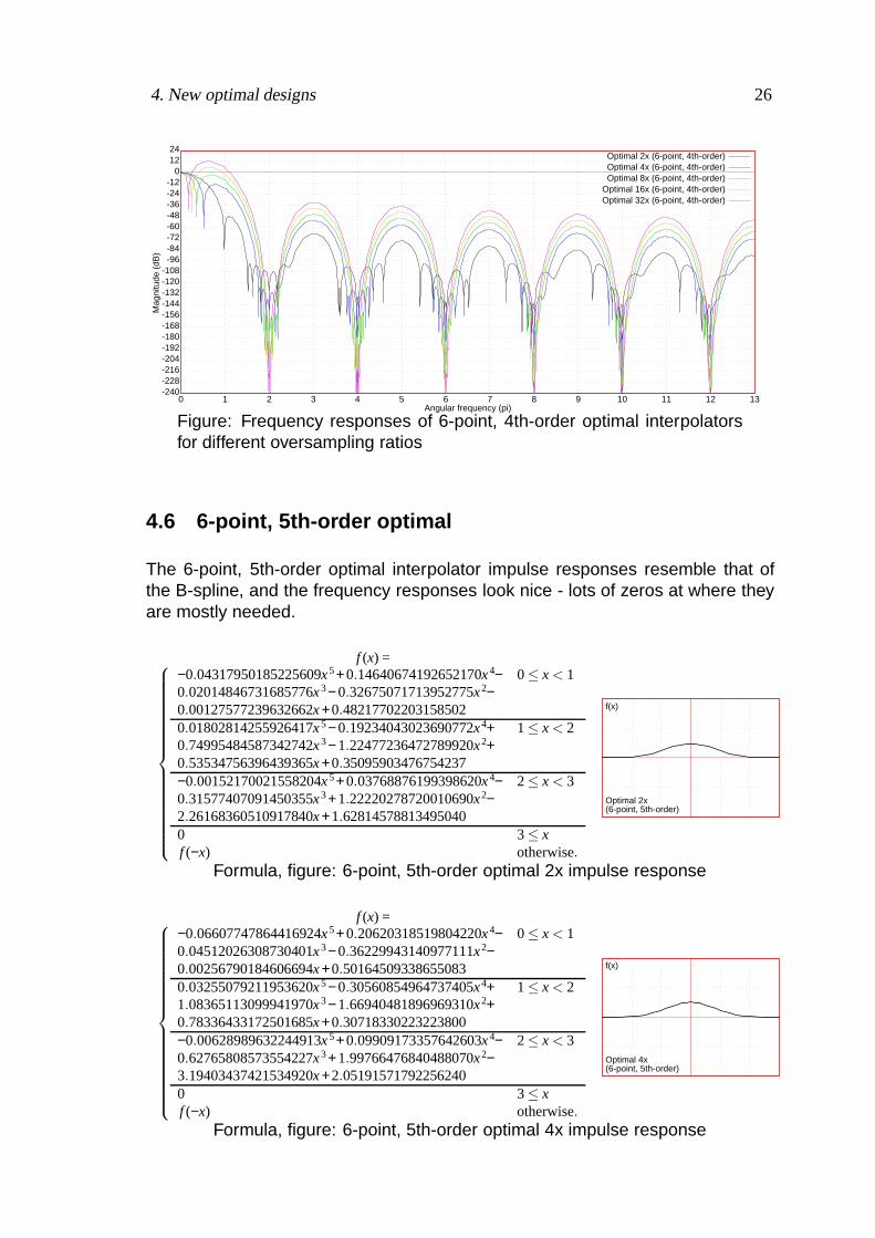
4. New optimal designs 26
-240-240-228-228-216-216-204-204-192-192-180-180-168-168-156-156-144-144-132-132-120-120-108-108-96-96-84-84-72-72-60-60-48-48-36-36-24-24-12-12
0012122424
00 11 22 33 44 55 66 77 88 99 1010 1111 1212 1313
Mag
nitu
de (
dB)
Mag
nitu
de (
dB)
Angular frequency (pi)Angular frequency (pi)
Optimal 2x (6-point, 4th-order)Optimal 2x (6-point, 4th-order)Optimal 4x (6-point, 4th-order)Optimal 4x (6-point, 4th-order)Optimal 8x (6-point, 4th-order)Optimal 8x (6-point, 4th-order)
Optimal 16x (6-point, 4th-order)Optimal 16x (6-point, 4th-order)Optimal 32x (6-point, 4th-order)Optimal 32x (6-point, 4th-order)
Figure: Frequency responses of 6-point, 4th-order optimal interpolatorsfor different oversampling ratios
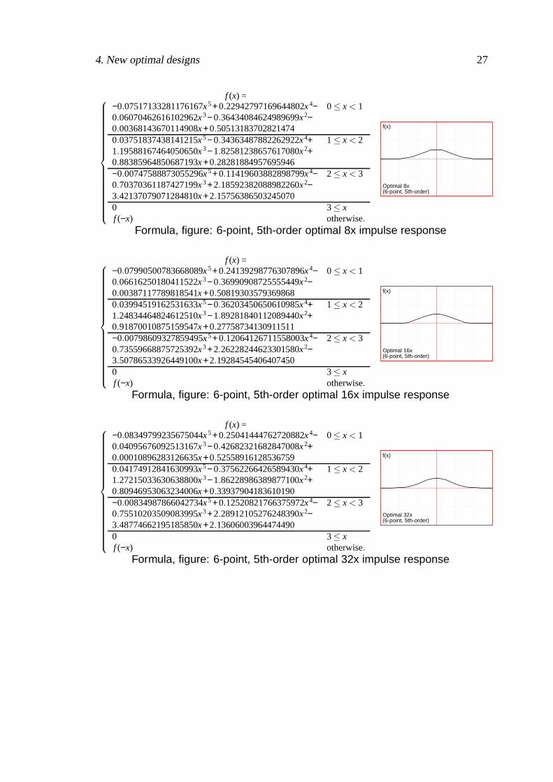
4.6 6-point, 5th-order optimal
The 6-point, 5th-order optimal interpolator impulse responses resemble that ofthe B-spline, and the frequency responses look nice - lots of zeros at where theyare mostly needed.
f (x) =
−0.04317950185225609x 5 +0.14640674192652170x 4− 0 ≤ x < 10.02014846731685776x 3 −0.32675071713952775x2−0.00127577239632662x +0.482177022031585020.01802814255926417x 5 −0.19234043023690772x4+ 1 ≤ x < 20.74995484587342742x 3 −1.22477236472789920x2+0.53534756396439365x +0.35095903476754237−0.00152170021558204x 5 +0.03768876199398620x 4− 2 ≤ x < 30.31577407091450355x 3 +1.22220278720010690x2−2.26168360510917840x +1.628145788134950400 3 ≤ xf (−x) otherwise.
f(x)f(x)
Optimal 2xOptimal 2x(6-point, 5th-order)(6-point, 5th-order)
Formula, figure: 6-point, 5th-order optimal 2x impulse response
f (x) =
−0.06607747864416924x 5 +0.20620318519804220x 4− 0 ≤ x < 10.04512026308730401x 3 −0.36229943140977111x2−0.00256790184606694x +0.501645093386550830.03255079211953620x 5 −0.30560854964737405x4+ 1 ≤ x < 21.08365113099941970x 3 −1.66940481896969310x2+0.78336433172501685x +0.30718330223223800−0.00628989632244913x 5 +0.09909173357642603x 4− 2 ≤ x < 30.62765808573554227x 3 +1.99766476840488070x2−3.19403437421534920x +2.051915717922562400 3 ≤ xf (−x) otherwise.
f(x)f(x)
Optimal 4xOptimal 4x(6-point, 5th-order)(6-point, 5th-order)
Formula, figure: 6-point, 5th-order optimal 4x impulse response
4. New optimal designs 27
f (x) =
−0.07517133281176167x 5 +0.22942797169644802x 4− 0 ≤ x < 10.06070462616102962x 3 −0.36434084624989699x2−0.00368143670114908x +0.505131837028214740.03751837438141215x 5 −0.34363487882262922x4+ 1 ≤ x < 21.19588167464050650x 3 −1.82581238657617080x2+0.88385964850687193x +0.28281884957695946−0.00747588873055296x 5 +0.11419603882898799x 4− 2 ≤ x < 30.70370361187427199x 3 +2.18592382088982260x2−3.42137079071284810x +2.157563865032450700 3 ≤ xf (−x) otherwise.
f(x)f(x)
Optimal 8xOptimal 8x(6-point, 5th-order)(6-point, 5th-order)
Formula, figure: 6-point, 5th-order optimal 8x impulse response
f (x) =
−0.07990500783668089x 5 +0.24139298776307896x 4− 0 ≤ x < 10.06616250180411522x 3 −0.36990908725555449x2−0.00387117789818541x +0.508193035793698680.03994519162531633x 5 −0.36203450650610985x4+ 1 ≤ x < 21.24834464824612510x 3 −1.89281840112089440x2+0.91870010875159547x +0.27758734130911511−0.00798609327859495x 5 +0.12064126711558003x 4− 2 ≤ x < 30.73559668875725392x 3 +2.26228244623301580x2−3.50786533926449100x +2.192845454064074500 3 ≤ xf (−x) otherwise.
f(x)f(x)
Optimal 16xOptimal 16x(6-point, 5th-order)(6-point, 5th-order)
Formula, figure: 6-point, 5th-order optimal 16x impulse response
f (x) =
−0.08349799235675044x 5 +0.25041444762720882x 4− 0 ≤ x < 10.04095676092513167x 3 −0.42682321682847008x2+0.00010896283126635x +0.525589161285367590.04174912841630993x 5 −0.37562266426589430x4+ 1 ≤ x < 21.27215033630638800x 3 −1.86228986389877100x2+0.80946953063234006x +0.33937904183610190−0.00834987866042734x 5 +0.12520821766375972x 4− 2 ≤ x < 30.75510203509083995x 3 +2.28912105276248390x2−3.48774662195185850x +2.136060039644744900 3 ≤ xf (−x) otherwise.
f(x)f(x)
Optimal 32xOptimal 32x(6-point, 5th-order)(6-point, 5th-order)
Formula, figure: 6-point, 5th-order optimal 32x impulse response
5. Comparison 28
-288-288-276-276-264-264-252-252-240-240-228-228-216-216-204-204-192-192-180-180-168-168-156-156-144-144-132-132-120-120-108-108-96-96-84-84-72-72-60-60-48-48-36-36-24-24-12-12
0012122424
00 11 22 33 44 55 66 77 88 99 1010 1111 1212 1313
Mag
nitu
de (
dB)
Mag
nitu
de (
dB)
Angular frequency (pi)Angular frequency (pi)
Optimal 2x (6-point, 5th-order)Optimal 2x (6-point, 5th-order)Optimal 4x (6-point, 5th-order)Optimal 4x (6-point, 5th-order)Optimal 8x (6-point, 5th-order)Optimal 8x (6-point, 5th-order)
Optimal 16x (6-point, 5th-order)Optimal 16x (6-point, 5th-order)Optimal 32x (6-point, 5th-order)Optimal 32x (6-point, 5th-order)
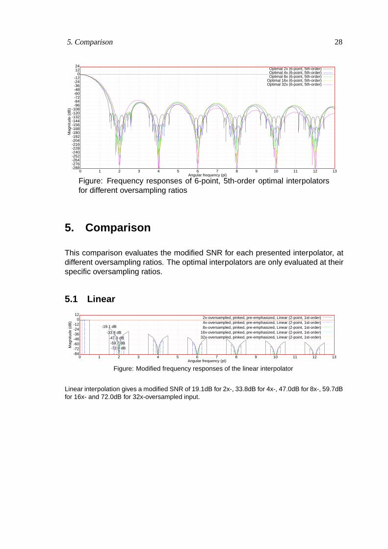
Figure: Frequency responses of 6-point, 5th-order optimal interpolatorsfor different oversampling ratios
5. Comparison
This comparison evaluates the modified SNR for each presented interpolator, atdifferent oversampling ratios. The optimal interpolators are only evaluated at theirspecific oversampling ratios.
5.1 Linear
-84-84-72-72-60-60-48-48-36-36-24-24-12-12
001212
00 11 22 33 44 55 66 77 88 99 1010 1111 1212 1313
Mag
nitu
de (
dB)
Mag
nitu
de (
dB)
Angular frequency (pi)Angular frequency (pi)
-19.1 dB-19.1 dB
2x-oversampled, pinked, pre-emphasized, Linear (2-point, 1st-order)2x-oversampled, pinked, pre-emphasized, Linear (2-point, 1st-order)
-33.8 dB-33.8 dB
4x-oversampled, pinked, pre-emphasized, Linear (2-point, 1st-order)4x-oversampled, pinked, pre-emphasized, Linear (2-point, 1st-order)
-47.0 dB-47.0 dB
8x-oversampled, pinked, pre-emphasized, Linear (2-point, 1st-order)8x-oversampled, pinked, pre-emphasized, Linear (2-point, 1st-order)
-59.7 dB-59.7 dB
16x-oversampled, pinked, pre-emphasized, Linear (2-point, 1st-order)16x-oversampled, pinked, pre-emphasized, Linear (2-point, 1st-order)
-72.0 dB-72.0 dB
32x-oversampled, pinked, pre-emphasized, Linear (2-point, 1st-order)32x-oversampled, pinked, pre-emphasized, Linear (2-point, 1st-order)
Figure: Modified frequency responses of the linear interpolator
Linear interpolation gives a modified SNR of 19.1dB for 2x-, 33.8dB for 4x-, 47.0dB for 8x-, 59.7dBfor 16x- and 72.0dB for 32x-oversampled input.
5. Comparison 29
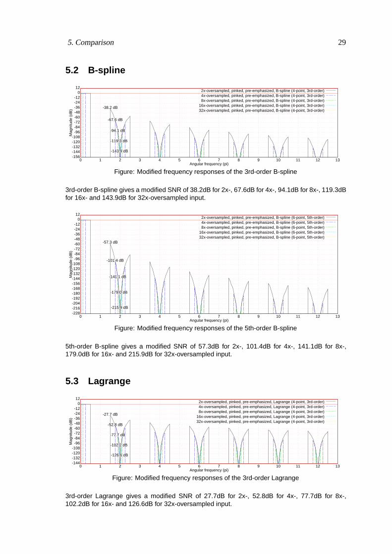
5.2 B-spline
-156-156-144-144-132-132-120-120-108-108-96-96-84-84-72-72-60-60-48-48-36-36-24-24-12-12
001212
00 11 22 33 44 55 66 77 88 99 1010 1111 1212 1313
Mag
nitu
de (
dB)
Mag
nitu
de (
dB)
Angular frequency (pi)Angular frequency (pi)
-38.2 dB-38.2 dB
2x-oversampled, pinked, pre-emphasized, B-spline (4-point, 3rd-order)2x-oversampled, pinked, pre-emphasized, B-spline (4-point, 3rd-order)
-67.6 dB-67.6 dB
4x-oversampled, pinked, pre-emphasized, B-spline (4-point, 3rd-order)4x-oversampled, pinked, pre-emphasized, B-spline (4-point, 3rd-order)
-94.1 dB-94.1 dB
8x-oversampled, pinked, pre-emphasized, B-spline (4-point, 3rd-order)8x-oversampled, pinked, pre-emphasized, B-spline (4-point, 3rd-order)
-119.3 dB-119.3 dB
16x-oversampled, pinked, pre-emphasized, B-spline (4-point, 3rd-order)16x-oversampled, pinked, pre-emphasized, B-spline (4-point, 3rd-order)
-143.9 dB-143.9 dB
32x-oversampled, pinked, pre-emphasized, B-spline (4-point, 3rd-order)32x-oversampled, pinked, pre-emphasized, B-spline (4-point, 3rd-order)
Figure: Modified frequency responses of the 3rd-order B-spline
3rd-order B-spline gives a modified SNR of 38.2dB for 2x-, 67.6dB for 4x-, 94.1dB for 8x-, 119.3dBfor 16x- and 143.9dB for 32x-oversampled input.
-228-228-216-216-204-204-192-192-180-180-168-168-156-156-144-144-132-132-120-120-108-108-96-96-84-84-72-72-60-60-48-48-36-36-24-24-12-12
001212
00 11 22 33 44 55 66 77 88 99 1010 1111 1212 1313
Mag
nitu
de (
dB)
Mag
nitu
de (
dB)
Angular frequency (pi)Angular frequency (pi)
-57.3 dB-57.3 dB
2x-oversampled, pinked, pre-emphasized, B-spline (6-point, 5th-order)2x-oversampled, pinked, pre-emphasized, B-spline (6-point, 5th-order)
-101.4 dB-101.4 dB
4x-oversampled, pinked, pre-emphasized, B-spline (6-point, 5th-order)4x-oversampled, pinked, pre-emphasized, B-spline (6-point, 5th-order)
-141.1 dB-141.1 dB
8x-oversampled, pinked, pre-emphasized, B-spline (6-point, 5th-order)8x-oversampled, pinked, pre-emphasized, B-spline (6-point, 5th-order)
-179.0 dB-179.0 dB
16x-oversampled, pinked, pre-emphasized, B-spline (6-point, 5th-order)16x-oversampled, pinked, pre-emphasized, B-spline (6-point, 5th-order)
-215.9 dB-215.9 dB
32x-oversampled, pinked, pre-emphasized, B-spline (6-point, 5th-order)32x-oversampled, pinked, pre-emphasized, B-spline (6-point, 5th-order)
Figure: Modified frequency responses of the 5th-order B-spline
5th-order B-spline gives a modified SNR of 57.3dB for 2x-, 101.4dB for 4x-, 141.1dB for 8x-,179.0dB for 16x- and 215.9dB for 32x-oversampled input.
5.3 Lagrange
-144-144-132-132-120-120-108-108-96-96-84-84-72-72-60-60-48-48-36-36-24-24-12-12
001212
00 11 22 33 44 55 66 77 88 99 1010 1111 1212 1313
Mag
nitu
de (
dB)
Mag
nitu
de (
dB)
Angular frequency (pi)Angular frequency (pi)
-27.7 dB-27.7 dB
2x-oversampled, pinked, pre-emphasized, Lagrange (4-point, 3rd-order)2x-oversampled, pinked, pre-emphasized, Lagrange (4-point, 3rd-order)
-52.8 dB-52.8 dB
4x-oversampled, pinked, pre-emphasized, Lagrange (4-point, 3rd-order)4x-oversampled, pinked, pre-emphasized, Lagrange (4-point, 3rd-order)
-77.7 dB-77.7 dB
8x-oversampled, pinked, pre-emphasized, Lagrange (4-point, 3rd-order)8x-oversampled, pinked, pre-emphasized, Lagrange (4-point, 3rd-order)
-102.2 dB-102.2 dB
16x-oversampled, pinked, pre-emphasized, Lagrange (4-point, 3rd-order)16x-oversampled, pinked, pre-emphasized, Lagrange (4-point, 3rd-order)
-126.6 dB-126.6 dB
32x-oversampled, pinked, pre-emphasized, Lagrange (4-point, 3rd-order)32x-oversampled, pinked, pre-emphasized, Lagrange (4-point, 3rd-order)
Figure: Modified frequency responses of the 3rd-order Lagrange
3rd-order Lagrange gives a modified SNR of 27.7dB for 2x-, 52.8dB for 4x-, 77.7dB for 8x-,102.2dB for 16x- and 126.6dB for 32x-oversampled input.
5. Comparison 30
-192-192-180-180-168-168-156-156-144-144-132-132-120-120-108-108-96-96-84-84-72-72-60-60-48-48-36-36-24-24-12-12
001212
00 11 22 33 44 55 66 77 88 99 1010 1111 1212 1313
Mag
nitu
de (
dB)
Mag
nitu
de (
dB)
Angular frequency (pi)Angular frequency (pi)
-35.2 dB-35.2 dB
2x-oversampled, pinked, pre-emphasized, Lagrange (6-point, 5th-order)2x-oversampled, pinked, pre-emphasized, Lagrange (6-point, 5th-order)
-70.9 dB-70.9 dB
4x-oversampled, pinked, pre-emphasized, Lagrange (6-point, 5th-order)4x-oversampled, pinked, pre-emphasized, Lagrange (6-point, 5th-order)
-107.5 dB-107.5 dB
8x-oversampled, pinked, pre-emphasized, Lagrange (6-point, 5th-order)8x-oversampled, pinked, pre-emphasized, Lagrange (6-point, 5th-order)
-144.1 dB-144.1 dB
16x-oversampled, pinked, pre-emphasized, Lagrange (6-point, 5th-order)16x-oversampled, pinked, pre-emphasized, Lagrange (6-point, 5th-order)
-180.5 dB-180.5 dB
32x-oversampled, pinked, pre-emphasized, Lagrange (6-point, 5th-order)32x-oversampled, pinked, pre-emphasized, Lagrange (6-point, 5th-order)
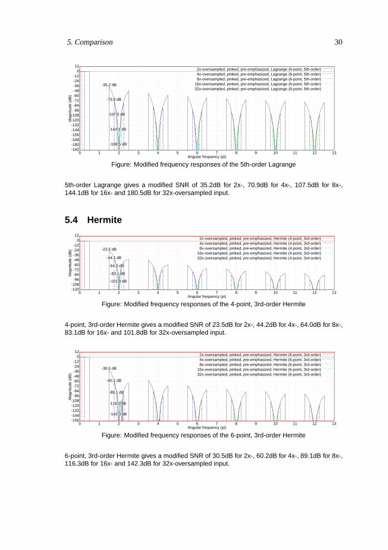
Figure: Modified frequency responses of the 5th-order Lagrange
5th-order Lagrange gives a modified SNR of 35.2dB for 2x-, 70.9dB for 4x-, 107.5dB for 8x-,144.1dB for 16x- and 180.5dB for 32x-oversampled input.
5.4 Hermite
-120-120-108-108-96-96-84-84-72-72-60-60-48-48-36-36-24-24-12-12
001212
00 11 22 33 44 55 66 77 88 99 1010 1111 1212 1313
Mag
nitu
de (
dB)
Mag
nitu
de (
dB)
Angular frequency (pi)Angular frequency (pi)
-23.5 dB-23.5 dB
2x-oversampled, pinked, pre-emphasized, Hermite (4-point, 3rd-order)2x-oversampled, pinked, pre-emphasized, Hermite (4-point, 3rd-order)
-44.2 dB-44.2 dB
4x-oversampled, pinked, pre-emphasized, Hermite (4-point, 3rd-order)4x-oversampled, pinked, pre-emphasized, Hermite (4-point, 3rd-order)
-64.0 dB-64.0 dB
8x-oversampled, pinked, pre-emphasized, Hermite (4-point, 3rd-order)8x-oversampled, pinked, pre-emphasized, Hermite (4-point, 3rd-order)
-83.1 dB-83.1 dB
16x-oversampled, pinked, pre-emphasized, Hermite (4-point, 3rd-order)16x-oversampled, pinked, pre-emphasized, Hermite (4-point, 3rd-order)
-101.8 dB-101.8 dB
32x-oversampled, pinked, pre-emphasized, Hermite (4-point, 3rd-order)32x-oversampled, pinked, pre-emphasized, Hermite (4-point, 3rd-order)
Figure: Modified frequency responses of the 4-point, 3rd-order Hermite
4-point, 3rd-order Hermite gives a modified SNR of 23.5dB for 2x-, 44.2dB for 4x-, 64.0dB for 8x-,83.1dB for 16x- and 101.8dB for 32x-oversampled input.
-156-156-144-144-132-132-120-120-108-108-96-96-84-84-72-72-60-60-48-48-36-36-24-24-12-12
001212
00 11 22 33 44 55 66 77 88 99 1010 1111 1212 1313
Mag
nitu
de (
dB)
Mag
nitu
de (
dB)
Angular frequency (pi)Angular frequency (pi)
-30.5 dB-30.5 dB
2x-oversampled, pinked, pre-emphasized, Hermite (6-point, 3rd-order)2x-oversampled, pinked, pre-emphasized, Hermite (6-point, 3rd-order)
-60.2 dB-60.2 dB
4x-oversampled, pinked, pre-emphasized, Hermite (6-point, 3rd-order)4x-oversampled, pinked, pre-emphasized, Hermite (6-point, 3rd-order)
-89.1 dB-89.1 dB
8x-oversampled, pinked, pre-emphasized, Hermite (6-point, 3rd-order)8x-oversampled, pinked, pre-emphasized, Hermite (6-point, 3rd-order)
-116.3 dB-116.3 dB
16x-oversampled, pinked, pre-emphasized, Hermite (6-point, 3rd-order)16x-oversampled, pinked, pre-emphasized, Hermite (6-point, 3rd-order)
-142.3 dB-142.3 dB
32x-oversampled, pinked, pre-emphasized, Hermite (6-point, 3rd-order)32x-oversampled, pinked, pre-emphasized, Hermite (6-point, 3rd-order)
Figure: Modified frequency responses of the 6-point, 3rd-order Hermite
6-point, 3rd-order Hermite gives a modified SNR of 30.5dB for 2x-, 60.2dB for 4x-, 89.1dB for 8x-,116.3dB for 16x- and 142.3dB for 32x-oversampled input.
5. Comparison 31
-168-168-156-156-144-144-132-132-120-120-108-108-96-96-84-84-72-72-60-60-48-48-36-36-24-24-12-12
001212
00 11 22 33 44 55 66 77 88 99 1010 1111 1212 1313
Mag
nitu
de (
dB)
Mag
nitu
de (
dB)
Angular frequency (pi)Angular frequency (pi)
-31.0 dB-31.0 dB
2x-oversampled, pinked, pre-emphasized, Hermite (6-point, 5th-order)2x-oversampled, pinked, pre-emphasized, Hermite (6-point, 5th-order)
-62.3 dB-62.3 dB
4x-oversampled, pinked, pre-emphasized, Hermite (6-point, 5th-order)4x-oversampled, pinked, pre-emphasized, Hermite (6-point, 5th-order)
-93.7 dB-93.7 dB
8x-oversampled, pinked, pre-emphasized, Hermite (6-point, 5th-order)8x-oversampled, pinked, pre-emphasized, Hermite (6-point, 5th-order)
-124.7 dB-124.7 dB
16x-oversampled, pinked, pre-emphasized, Hermite (6-point, 5th-order)16x-oversampled, pinked, pre-emphasized, Hermite (6-point, 5th-order)
-155.4 dB-155.4 dB
32x-oversampled, pinked, pre-emphasized, Hermite (6-point, 5th-order)32x-oversampled, pinked, pre-emphasized, Hermite (6-point, 5th-order)
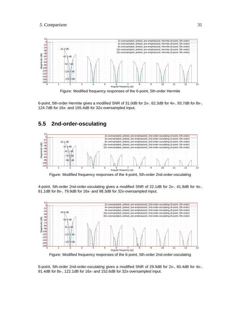
Figure: Modified frequency responses of the 6-point, 5th-order Hermite
6-point, 5th-order Hermite gives a modified SNR of 31.0dB for 2x-, 62.3dB for 4x-, 93.7dB for 8x-,124.7dB for 16x- and 155.4dB for 32x-oversampled input.
5.5 2nd-order-osculating
-120-120-108-108-96-96-84-84-72-72-60-60-48-48-36-36-24-24-12-12
001212
00 11 22 33 44 55 66 77 88 99 1010 1111 1212 1313
Mag
nitu
de (
dB)
Mag
nitu
de (
dB)
Angular frequency (pi)Angular frequency (pi)
-22.1 dB-22.1 dB
2x-oversampled, pinked, pre-emphasized, 2nd-order-osculating (4-point, 5th-order)2x-oversampled, pinked, pre-emphasized, 2nd-order-osculating (4-point, 5th-order)
-41.9 dB-41.9 dB
4x-oversampled, pinked, pre-emphasized, 2nd-order-osculating (4-point, 5th-order)4x-oversampled, pinked, pre-emphasized, 2nd-order-osculating (4-point, 5th-order)
-61.1 dB-61.1 dB
8x-oversampled, pinked, pre-emphasized, 2nd-order-osculating (4-point, 5th-order)8x-oversampled, pinked, pre-emphasized, 2nd-order-osculating (4-point, 5th-order)
-79.9 dB-79.9 dB
16x-oversampled, pinked, pre-emphasized, 2nd-order-osculating (4-point, 5th-order)16x-oversampled, pinked, pre-emphasized, 2nd-order-osculating (4-point, 5th-order)
-98.3 dB-98.3 dB
32x-oversampled, pinked, pre-emphasized, 2nd-order-osculating (4-point, 5th-order)32x-oversampled, pinked, pre-emphasized, 2nd-order-osculating (4-point, 5th-order)
Figure: Modified frequency responses of the 4-point, 5th-order 2nd-order-osculating
4-point, 5th-order 2nd-order-osculating gives a modified SNR of 22.1dB for 2x-, 41.9dB for 4x-,61.1dB for 8x-, 79.9dB for 16x- and 98.3dB for 32x-oversampled input.
-168-168-156-156-144-144-132-132-120-120-108-108-96-96-84-84-72-72-60-60-48-48-36-36-24-24-12-12
001212
00 11 22 33 44 55 66 77 88 99 1010 1111 1212 1313
Mag
nitu
de (
dB)
Mag
nitu
de (
dB)
Angular frequency (pi)Angular frequency (pi)
-29.9 dB-29.9 dB
2x-oversampled, pinked, pre-emphasized, 2nd-order-osculating (6-point, 5th-order)2x-oversampled, pinked, pre-emphasized, 2nd-order-osculating (6-point, 5th-order)
-60.4 dB-60.4 dB
4x-oversampled, pinked, pre-emphasized, 2nd-order-osculating (6-point, 5th-order)4x-oversampled, pinked, pre-emphasized, 2nd-order-osculating (6-point, 5th-order)
-91.4 dB-91.4 dB
8x-oversampled, pinked, pre-emphasized, 2nd-order-osculating (6-point, 5th-order)8x-oversampled, pinked, pre-emphasized, 2nd-order-osculating (6-point, 5th-order)
-122.1 dB-122.1 dB
16x-oversampled, pinked, pre-emphasized, 2nd-order-osculating (6-point, 5th-order)16x-oversampled, pinked, pre-emphasized, 2nd-order-osculating (6-point, 5th-order)
-152.6 dB-152.6 dB
32x-oversampled, pinked, pre-emphasized, 2nd-order-osculating (6-point, 5th-order)32x-oversampled, pinked, pre-emphasized, 2nd-order-osculating (6-point, 5th-order)
Figure: Modified frequency responses of the 6-point, 5th-order 2nd-order-osculating
6-point, 5th-order 2nd-order-osculating gives a modified SNR of 29.9dB for 2x-, 60.4dB for 4x-,91.4dB for 8x-, 122.1dB for 16x- and 152.6dB for 32x-oversampled input.

5. Comparison 32
5.6 Watte tri-linear
-84-84-72-72-60-60-48-48-36-36-24-24-12-12
001212
00 11 22 33 44 55 66 77 88 99 1010 1111 1212 1313
Mag
nitu
de (
dB)
Mag
nitu
de (
dB)
Angular frequency (pi)Angular frequency (pi)
-27.9 dB-27.9 dB
2x-oversampled, pinked, pre-emphasized, Watte tri-linear (4-point, 2nd-order)2x-oversampled, pinked, pre-emphasized, Watte tri-linear (4-point, 2nd-order)
-34.9 dB-34.9 dB
4x-oversampled, pinked, pre-emphasized, Watte tri-linear (4-point, 2nd-order)4x-oversampled, pinked, pre-emphasized, Watte tri-linear (4-point, 2nd-order)
-46.8 dB-46.8 dB
8x-oversampled, pinked, pre-emphasized, Watte tri-linear (4-point, 2nd-order)8x-oversampled, pinked, pre-emphasized, Watte tri-linear (4-point, 2nd-order)
-59.3 dB-59.3 dB
16x-oversampled, pinked, pre-emphasized, Watte tri-linear (4-point, 2nd-order)16x-oversampled, pinked, pre-emphasized, Watte tri-linear (4-point, 2nd-order)
-71.8 dB-71.8 dB
32x-oversampled, pinked, pre-emphasized, Watte tri-linear (4-point, 2nd-order)32x-oversampled, pinked, pre-emphasized, Watte tri-linear (4-point, 2nd-order)
Figure: Modified frequency responses of the Watte tri-linear
Watte tri-linear gives a modified SNR of 27.9dB for 2x-, 34.9dB for 4x-, 46.8dB for 8x-, 59.3dB for16x- and 71.8dB for 32x-oversampled input.
5.7 Parabolic 2x
-120-120-108-108-96-96-84-84-72-72-60-60-48-48-36-36-24-24-12-12
001212
00 11 22 33 44 55 66 77 88 99 1010 1111 1212 1313
Mag
nitu
de (
dB)
Mag
nitu
de (
dB)
Angular frequency (pi)Angular frequency (pi)
-28.6 dB-28.6 dB
2x-oversampled, pinked, pre-emphasized, Parabolic 2x (4-point, 2nd-order)2x-oversampled, pinked, pre-emphasized, Parabolic 2x (4-point, 2nd-order)
-50.7 dB-50.7 dB
4x-oversampled, pinked, pre-emphasized, Parabolic 2x (4-point, 2nd-order)4x-oversampled, pinked, pre-emphasized, Parabolic 2x (4-point, 2nd-order)
-70.6 dB-70.6 dB
8x-oversampled, pinked, pre-emphasized, Parabolic 2x (4-point, 2nd-order)8x-oversampled, pinked, pre-emphasized, Parabolic 2x (4-point, 2nd-order)
-89.5 dB-89.5 dB
16x-oversampled, pinked, pre-emphasized, Parabolic 2x (4-point, 2nd-order)16x-oversampled, pinked, pre-emphasized, Parabolic 2x (4-point, 2nd-order)
-108.0 dB-108.0 dB
32x-oversampled, pinked, pre-emphasized, Parabolic 2x (4-point, 2nd-order)32x-oversampled, pinked, pre-emphasized, Parabolic 2x (4-point, 2nd-order)
Figure: Modified frequency responses of the parabolic 2x
Parabolic 2x gives a modified SNR of 28.6dB for 2x-, 50.7dB for 4x-, 70.6dB for 8x-, 89.5dB for16x- and 108.0dB for 32x-oversampled input.
5.8 Optimal
-84-84-72-72-60-60-48-48-36-36-24-24-12-12
0012122424
00 11 22 33 44 55 66 77 88 99 1010 1111 1212 1313
Mag
nitu
de (
dB)
Mag
nitu
de (
dB)
Angular frequency (pi)Angular frequency (pi)
-28.0 dB-28.0 dB
2x-oversampled, pinked, pre-emphasized, Optimal 2x (2-point, 3rd-order)2x-oversampled, pinked, pre-emphasized, Optimal 2x (2-point, 3rd-order)
-39.1 dB-39.1 dB
4x-oversampled, pinked, pre-emphasized, Optimal 4x (2-point, 3rd-order)4x-oversampled, pinked, pre-emphasized, Optimal 4x (2-point, 3rd-order)
-49.7 dB-49.7 dB
8x-oversampled, pinked, pre-emphasized, Optimal 8x (2-point, 3rd-order)8x-oversampled, pinked, pre-emphasized, Optimal 8x (2-point, 3rd-order)
-61.0 dB-61.0 dB
16x-oversampled, pinked, pre-emphasized, Optimal 16x (2-point, 3rd-order)16x-oversampled, pinked, pre-emphasized, Optimal 16x (2-point, 3rd-order)
-72.7 dB-72.7 dB
32x-oversampled, pinked, pre-emphasized, Optimal 32x (2-point, 3rd-order)32x-oversampled, pinked, pre-emphasized, Optimal 32x (2-point, 3rd-order)
Figure: Modified frequency responses of the 2-point, 3rd-order optimal interpolators
2-point, 3rd-order optimal interpolators give modified SNRs of 28.0dB for 2x-, 39.1dB for 4x-,49.7dB for 8x-, 61.0dB for 16x- and 72.7dB for 32x-oversampled input.
5. Comparison 33
-132-132-120-120-108-108-96-96-84-84-72-72-60-60-48-48-36-36-24-24-12-12
001212
00 11 22 33 44 55 66 77 88 99 1010 1111 1212 1313
Mag
nitu
de (
dB)
Mag
nitu
de (
dB)
Angular frequency (pi)Angular frequency (pi)
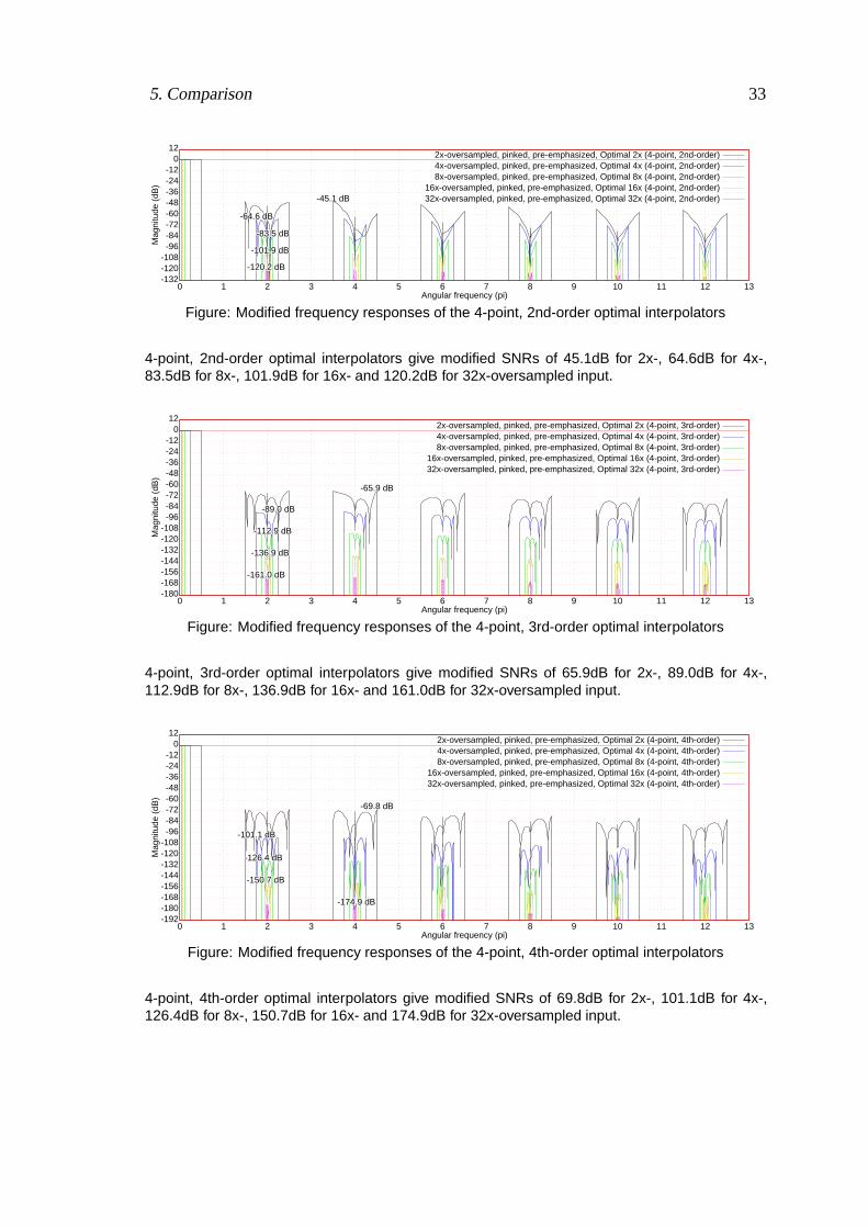
-45.1 dB-45.1 dB
2x-oversampled, pinked, pre-emphasized, Optimal 2x (4-point, 2nd-order)2x-oversampled, pinked, pre-emphasized, Optimal 2x (4-point, 2nd-order)
-64.6 dB-64.6 dB
4x-oversampled, pinked, pre-emphasized, Optimal 4x (4-point, 2nd-order)4x-oversampled, pinked, pre-emphasized, Optimal 4x (4-point, 2nd-order)
-83.5 dB-83.5 dB
8x-oversampled, pinked, pre-emphasized, Optimal 8x (4-point, 2nd-order)8x-oversampled, pinked, pre-emphasized, Optimal 8x (4-point, 2nd-order)
-101.9 dB-101.9 dB
16x-oversampled, pinked, pre-emphasized, Optimal 16x (4-point, 2nd-order)16x-oversampled, pinked, pre-emphasized, Optimal 16x (4-point, 2nd-order)
-120.2 dB-120.2 dB
32x-oversampled, pinked, pre-emphasized, Optimal 32x (4-point, 2nd-order)32x-oversampled, pinked, pre-emphasized, Optimal 32x (4-point, 2nd-order)
Figure: Modified frequency responses of the 4-point, 2nd-order optimal interpolators
4-point, 2nd-order optimal interpolators give modified SNRs of 45.1dB for 2x-, 64.6dB for 4x-,83.5dB for 8x-, 101.9dB for 16x- and 120.2dB for 32x-oversampled input.
-180-180-168-168-156-156-144-144-132-132-120-120-108-108-96-96-84-84-72-72-60-60-48-48-36-36-24-24-12-12
001212
00 11 22 33 44 55 66 77 88 99 1010 1111 1212 1313
Mag
nitu
de (
dB)
Mag
nitu
de (
dB)
Angular frequency (pi)Angular frequency (pi)
-65.9 dB-65.9 dB
2x-oversampled, pinked, pre-emphasized, Optimal 2x (4-point, 3rd-order)2x-oversampled, pinked, pre-emphasized, Optimal 2x (4-point, 3rd-order)
-89.0 dB-89.0 dB
4x-oversampled, pinked, pre-emphasized, Optimal 4x (4-point, 3rd-order)4x-oversampled, pinked, pre-emphasized, Optimal 4x (4-point, 3rd-order)
-112.9 dB-112.9 dB
8x-oversampled, pinked, pre-emphasized, Optimal 8x (4-point, 3rd-order)8x-oversampled, pinked, pre-emphasized, Optimal 8x (4-point, 3rd-order)
-136.9 dB-136.9 dB
16x-oversampled, pinked, pre-emphasized, Optimal 16x (4-point, 3rd-order)16x-oversampled, pinked, pre-emphasized, Optimal 16x (4-point, 3rd-order)
-161.0 dB-161.0 dB
32x-oversampled, pinked, pre-emphasized, Optimal 32x (4-point, 3rd-order)32x-oversampled, pinked, pre-emphasized, Optimal 32x (4-point, 3rd-order)
Figure: Modified frequency responses of the 4-point, 3rd-order optimal interpolators
4-point, 3rd-order optimal interpolators give modified SNRs of 65.9dB for 2x-, 89.0dB for 4x-,112.9dB for 8x-, 136.9dB for 16x- and 161.0dB for 32x-oversampled input.
-192-192-180-180-168-168-156-156-144-144-132-132-120-120-108-108-96-96-84-84-72-72-60-60-48-48-36-36-24-24-12-12
001212
00 11 22 33 44 55 66 77 88 99 1010 1111 1212 1313
Mag
nitu
de (
dB)
Mag
nitu
de (
dB)
Angular frequency (pi)Angular frequency (pi)
-69.8 dB-69.8 dB
2x-oversampled, pinked, pre-emphasized, Optimal 2x (4-point, 4th-order)2x-oversampled, pinked, pre-emphasized, Optimal 2x (4-point, 4th-order)
-101.1 dB-101.1 dB
4x-oversampled, pinked, pre-emphasized, Optimal 4x (4-point, 4th-order)4x-oversampled, pinked, pre-emphasized, Optimal 4x (4-point, 4th-order)
-126.4 dB-126.4 dB
8x-oversampled, pinked, pre-emphasized, Optimal 8x (4-point, 4th-order)8x-oversampled, pinked, pre-emphasized, Optimal 8x (4-point, 4th-order)
-150.7 dB-150.7 dB
16x-oversampled, pinked, pre-emphasized, Optimal 16x (4-point, 4th-order)16x-oversampled, pinked, pre-emphasized, Optimal 16x (4-point, 4th-order)
-174.9 dB-174.9 dB
32x-oversampled, pinked, pre-emphasized, Optimal 32x (4-point, 4th-order)32x-oversampled, pinked, pre-emphasized, Optimal 32x (4-point, 4th-order)
Figure: Modified frequency responses of the 4-point, 4th-order optimal interpolators
4-point, 4th-order optimal interpolators give modified SNRs of 69.8dB for 2x-, 101.1dB for 4x-,126.4dB for 8x-, 150.7dB for 16x- and 174.9dB for 32x-oversampled input.
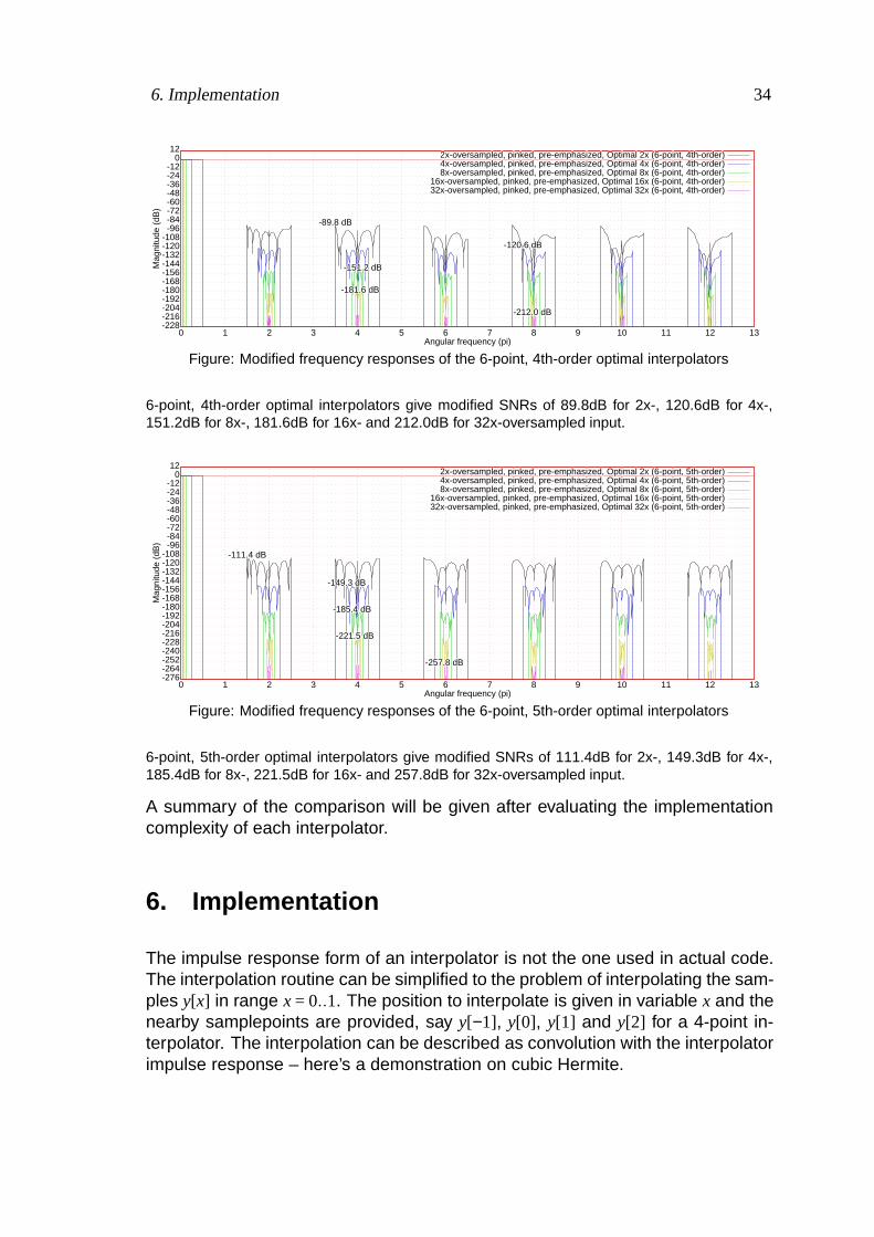
6. Implementation 34
-228-228-216-216-204-204-192-192-180-180-168-168-156-156-144-144-132-132-120-120-108-108-96-96-84-84-72-72-60-60-48-48-36-36-24-24-12-12
001212
00 11 22 33 44 55 66 77 88 99 1010 1111 1212 1313
Mag
nitu
de (
dB)
Mag
nitu
de (
dB)
Angular frequency (pi)Angular frequency (pi)
-89.8 dB-89.8 dB
2x-oversampled, pinked, pre-emphasized, Optimal 2x (6-point, 4th-order)2x-oversampled, pinked, pre-emphasized, Optimal 2x (6-point, 4th-order)
-120.6 dB-120.6 dB
4x-oversampled, pinked, pre-emphasized, Optimal 4x (6-point, 4th-order)4x-oversampled, pinked, pre-emphasized, Optimal 4x (6-point, 4th-order)
-151.2 dB-151.2 dB
8x-oversampled, pinked, pre-emphasized, Optimal 8x (6-point, 4th-order)8x-oversampled, pinked, pre-emphasized, Optimal 8x (6-point, 4th-order)
-181.6 dB-181.6 dB
16x-oversampled, pinked, pre-emphasized, Optimal 16x (6-point, 4th-order)16x-oversampled, pinked, pre-emphasized, Optimal 16x (6-point, 4th-order)
-212.0 dB-212.0 dB
32x-oversampled, pinked, pre-emphasized, Optimal 32x (6-point, 4th-order)32x-oversampled, pinked, pre-emphasized, Optimal 32x (6-point, 4th-order)
Figure: Modified frequency responses of the 6-point, 4th-order optimal interpolators
6-point, 4th-order optimal interpolators give modified SNRs of 89.8dB for 2x-, 120.6dB for 4x-,151.2dB for 8x-, 181.6dB for 16x- and 212.0dB for 32x-oversampled input.
-276-276-264-264-252-252-240-240-228-228-216-216-204-204-192-192-180-180-168-168-156-156-144-144-132-132-120-120-108-108-96-96-84-84-72-72-60-60-48-48-36-36-24-24-12-12
001212
00 11 22 33 44 55 66 77 88 99 1010 1111 1212 1313
Mag
nitu
de (
dB)
Mag
nitu
de (
dB)
Angular frequency (pi)Angular frequency (pi)
-111.4 dB-111.4 dB
2x-oversampled, pinked, pre-emphasized, Optimal 2x (6-point, 5th-order)2x-oversampled, pinked, pre-emphasized, Optimal 2x (6-point, 5th-order)
-149.3 dB-149.3 dB
4x-oversampled, pinked, pre-emphasized, Optimal 4x (6-point, 5th-order)4x-oversampled, pinked, pre-emphasized, Optimal 4x (6-point, 5th-order)
-185.4 dB-185.4 dB
8x-oversampled, pinked, pre-emphasized, Optimal 8x (6-point, 5th-order)8x-oversampled, pinked, pre-emphasized, Optimal 8x (6-point, 5th-order)
-221.5 dB-221.5 dB
16x-oversampled, pinked, pre-emphasized, Optimal 16x (6-point, 5th-order)16x-oversampled, pinked, pre-emphasized, Optimal 16x (6-point, 5th-order)
-257.8 dB-257.8 dB
32x-oversampled, pinked, pre-emphasized, Optimal 32x (6-point, 5th-order)32x-oversampled, pinked, pre-emphasized, Optimal 32x (6-point, 5th-order)
Figure: Modified frequency responses of the 6-point, 5th-order optimal interpolators
6-point, 5th-order optimal interpolators give modified SNRs of 111.4dB for 2x-, 149.3dB for 4x-,185.4dB for 8x-, 221.5dB for 16x- and 257.8dB for 32x-oversampled input.
A summary of the comparison will be given after evaluating the implementationcomplexity of each interpolator.
6. Implementation
The impulse response form of an interpolator is not the one used in actual code.The interpolation routine can be simplified to the problem of interpolating the sam-ples y[x] in range x = 0..1. The position to interpolate is given in variable x and thenearby samplepoints are provided, say y[−1], y[0], y[1] and y[2] for a 4-point in-terpolator. The interpolation can be described as convolution with the interpolatorimpulse response – here’s a demonstration on cubic Hermite.
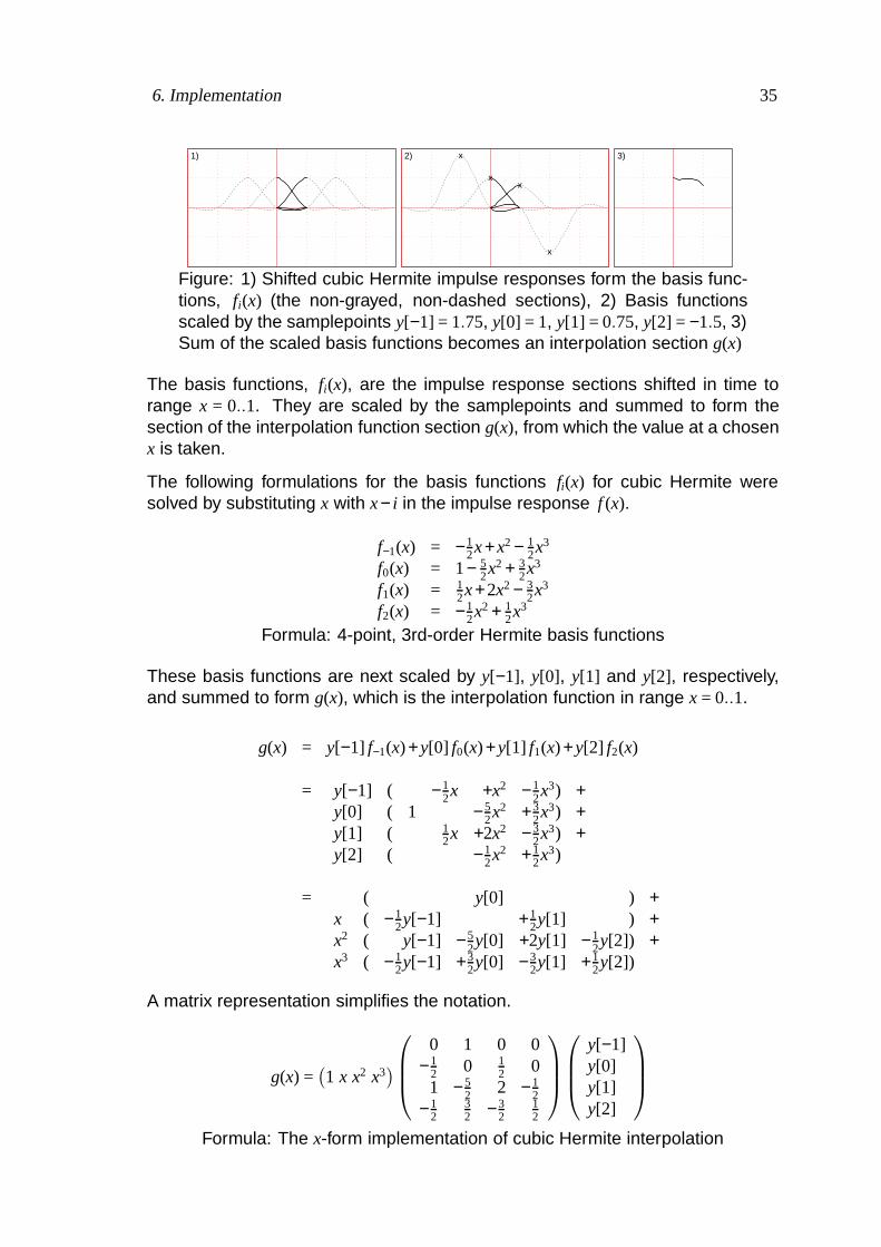
6. Implementation 35
x
x
x
x
1) 2) 3)
Figure: 1) Shifted cubic Hermite impulse responses form the basis func-tions, fi(x) (the non-grayed, non-dashed sections), 2) Basis functionsscaled by the samplepoints y[−1] = 1.75, y[0] = 1, y[1] = 0.75, y[2] = −1.5, 3)Sum of the scaled basis functions becomes an interpolation section g(x)
The basis functions, fi(x), are the impulse response sections shifted in time torange x = 0..1. They are scaled by the samplepoints and summed to form thesection of the interpolation function section g(x), from which the value at a chosenx is taken.
The following formulations for the basis functions fi(x) for cubic Hermite weresolved by substituting x with x − i in the impulse response f (x).
f−1(x) = −12x +x2 − 1
2x3
f0(x) = 1 − 52x2 + 3
2x3
f1(x) = 12x +2x2 − 3
2x3
f2(x) = −12x2 + 1
2x3
Formula: 4-point, 3rd-order Hermite basis functions
These basis functions are next scaled by y[−1], y[0], y[1] and y[2], respectively,and summed to form g(x), which is the interpolation function in range x = 0..1.
g(x) = y[−1] f−1(x) +y[0] f0(x) +y[1] f1(x) +y[2] f2(x)
= y[−1] ( −12x +x2 −1
2x3) +y[0] ( 1 −5
2x2 +32x3) +
y[1] ( 12x +2x2 −3
2x3) +y[2] ( −1
2x2 +12x3)
= ( y[0] ) +x ( −1
2y[−1] +12y[1] ) +
x2 ( y[−1] −52y[0] +2y[1] −1
2y[2]) +x3 ( −1
2y[−1] +32y[0] −3
2y[1] +12y[2])
A matrix representation simplifies the notation.
g(x) =(1 x x2 x3
)
0 1 0 0−1
2 0 12 0
1 −52 2 −1
2−1
232 −3
212
y[−1]y[0]y[1]y[2]
Formula: The x-form implementation of cubic Hermite interpolation

6. Implementation 36
In the coefficient matrix, if there are numbers on a row that have the same ab-solute value, the corresponding multiplications can be combined, increasing thespeed of the interpolation routine. The symmetry of the impulse responses canbe exploited to limit the number of required multiplications to half the number ofmatrix elements, or below if we are lucky, by a substitution x = 1
2 + z, which shiftsthe symmetry axis to z = 0. This trick may not be effective for matrices that al-ready have many pairable elements, zeros or minus or plus ones that need notbe multiplied. Nevertheless, we shall demonstrate this on the cubic Hermite.
g(x) =(1 z z2 z3
)
− 116
916
916 − 1
1618 −11
8118 −1
814 −1
4 −14
14
−12
32 −3
212
y[−1]y[0]y[1]y[2]
, z = x − 1
2
Formula: The z-form implementation of cubic Hermite interpolation
We shall call these implementations the x- and the z-form, and their coefficientmatrices X and Z, respectively. With cubic Hermite, the x-form requires 6 multi-plications to calculate the polynomial g(x) coefficients, and the z-form requires 7.So, for cubic Hermite, it is better to use the x-form given earlier.
After the coefficients have been computed, the interpolation polynomial g(x) mustbe evaluated. Horner’s rule can be used to reduce multiplications, for example:
c3x3 +c2x2 +c1x +c0 = ((c3x +c2)x +c1)x +c0
Formula: Horner’s rule
So evaluating a polynomial requires the same number of multiplications its or-der is. Summing this number with the number of multiplications required by thecheaper matrix-vector multiplication (x-form for cubic Hermite) gives the total num-ber of multiplications required (9 for cubic Hermite). It should be noted, however,that on some platforms, using Horner’s rule is not beneficial, so feel free to modifythe source codes given later.
Next we shall try finding the best implementation form for each interpolator.
To choose between the x- and the z-form, we find out the number of operationsin both. First we find out which needs more multiplications. If multiplications areexpensive on the target platform, then that is what matters. However, if multiplica-tions are as cheap as addition and subtraction operations, then the total numberof operations counts. Optimized C language source code for the x- and z-formalgorithms is given in the following, and the total number of operations is countedfrom each.
Looking at the matrices X and Z, some of the coefficients can be paired. This ismarked with blue color, and two such coefficients require only one multiplication.Usually, the pair can be found from the same row, but sometimes on the same

6. Implementation 37
column. If more coefficients can be combined into larger groups that reducemultiplications, they are marked with red color. The Z-matrices have all rowseither symmetrical or antisymmetrical, so pairing is guaranteed.
Zeros and plus and minus ones require no multiplications. If a coefficient is oth-erwise trivial, for example 1
8 , the multiplication might be possible to perform witha binary shift operation. In this paper, however, a floating point platform with nosuch scaling command is presumed and coefficients like that are treated as usual.
6.1 Linear
Linear interpolation is best done simply as:
g(x) = y[0] +x(y[1] −y[0])
Formula: Linear interpolation implementation
requiring total 1 multiplication.
// Linearreturn y[0] + x*(y[1]-y[0]);
Routine: Linear interpolation implementation
The total number of operations in the routine is 3 (1 mul, 2 adds/subs).
6.2 B-spline
X =
16
23
16 0
−12 0 1
2 012 −1 1
2 0−1
612 −1
216
, Z =
148
2348
2348
148
−18 −5
858
18
14 −1
4 −14
14
−16
12 −1
216
Formula: 4-point, 3rd-order B-spline x- and z-form coefficient matrices
For 4-point, 3rd-order B-spline, X requires 6 multiplications and Z requires 7. Notethat the polynomial evaluation requires some more, but the number is typicallysame for both the x- and the z-form of an interpolator.
// 4-point, 3rd-order B-spline (x-form)float ym1py1 = y[-1]+y[1];float c0 = 1/6.0*ym1py1 + 2/3.0*y[0];float c1 = 1/2.0*(y[1]-y[-1]);float c2 = 1/2.0*ym1py1 - y[0];float c3 = 1/2.0*(y[0]-y[1]) + 1/6.0*(y[2]-y[-1]);return ((c3*x+c2)*x+c1)*x+c0;
Routine: 4-point, 3rd-order B-spline x-form implementation

6. Implementation 38
// 4-point, 3rd-order B-spline (z-form)float z = x - 1/2.0;float even1 = y[-1]+y[2], modd1 = y[2]-y[-1];float even2 = y[0]+y[1], modd2 = y[1]-y[0];float c0 = 1/48.0*even1 + 23/48.0*even2;float c1 = 1/8.0*modd1 + 5/8.0*modd2;float c2 = 1/4.0*(even1-even2);float c3 = 1/6.0*modd1 - 1/2.0*modd2;return ((c3*z+c2)*z+c1)*z+c0;
Routine: 4-point, 3rd-order B-spline z-form implementation
For 4-point, 3rd-order B-spline, the total number of operations in the x-form routineis 19 (9 muls, 10 adds/subs) and in the z-form 22 (10 muls, 12 adds/subs), so thex-form is favorable.
X =
1120
1360
1120
1360
1120 0
− 124 − 5
12 0 512
124 0
112
16 −1
216
112 0
− 112
16 0 −1
6112 0
124 −1
614 −1
6124 0
− 1120
124 − 1
12112 − 1
241
120
Z =
13840
791280
8411920
8411920
791280
13840
− 1384 − 25
128 − 77192
77192
25128
1384
196
732 −11
48 −1148
732
196
− 148 − 1
167
24 − 724
116
148
148 − 1
161
24124 − 1
161
48− 1
120124 − 1
12112 − 1
241
120
Formula: 6-point, 5th-order B-spline x- and z-form coefficient matrices
For 6-point, 5th-order B-spline, X requires 15 multiplications against the 18 of Z,so the x-form is probably more favorable.
// 6-point, 5th-order B-spline (x-form)float ym2py2 = y[-2]+y[2], ym1py1 = y[-1]+y[1];float y2mym2 = y[2]-y[-2], y1mym1 = y[1]-y[-1];float sixthym1py1 = 1/6.0*ym1py1;float c0 = 1/120.0*ym2py2 + 13/60.0*ym1py1 + 11/20.0*y[0];float c1 = 1/24.0*y2mym2 + 5/12.0*y1mym1;float c2 = 1/12.0*ym2py2 + sixthym1py1 - 1/2.0*y[0];float c3 = 1/12.0*y2mym2 - 1/6.0*y1mym1;float c4 = 1/24.0*ym2py2 - sixthym1py1 + 1/4.0*y[0];float c5 = 1/120.0*(y[3]-y[-2]) + 1/24.0*(y[-1]-y[2]) +
1/12.0*(y[1]-y[0]);return ((((c5*x+c4)*x+c3)*x+c2)*x+c1)*x+c0;
Routine: 6-point, 5th-order B-spline x-form implementation
For 6-point, 5th-order B-spline, the total number of operations in the x-form routineis 42 (20 mul, 22 add/sub). There is a rule that a z-form routine with only pairing,no larger grouping, requires order× (points+1)+2× points operations total. In thiscase, the z-form would require 47 operations, so the x-form is a clear winner.
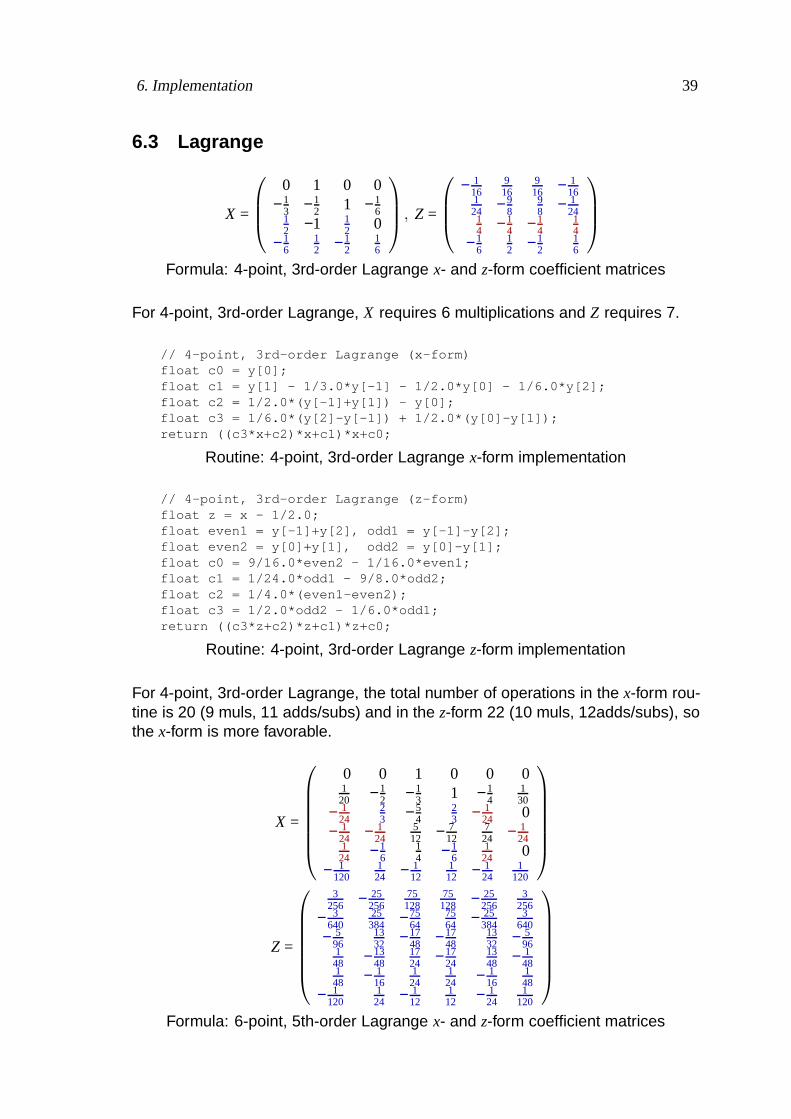
6. Implementation 39
6.3 Lagrange
X =
0 1 0 0−1
3 −12 1 −1
612 −1 1
2 0−1
612 −1
216
, Z =
− 116
916
916 − 1
16124 −9
898 − 1
2414 −1
4 −14
14
−16
12 −1
216
Formula: 4-point, 3rd-order Lagrange x- and z-form coefficient matrices
For 4-point, 3rd-order Lagrange, X requires 6 multiplications and Z requires 7.
// 4-point, 3rd-order Lagrange (x-form)float c0 = y[0];float c1 = y[1] - 1/3.0*y[-1] - 1/2.0*y[0] - 1/6.0*y[2];float c2 = 1/2.0*(y[-1]+y[1]) - y[0];float c3 = 1/6.0*(y[2]-y[-1]) + 1/2.0*(y[0]-y[1]);return ((c3*x+c2)*x+c1)*x+c0;
Routine: 4-point, 3rd-order Lagrange x-form implementation
// 4-point, 3rd-order Lagrange (z-form)float z = x - 1/2.0;float even1 = y[-1]+y[2], odd1 = y[-1]-y[2];float even2 = y[0]+y[1], odd2 = y[0]-y[1];float c0 = 9/16.0*even2 - 1/16.0*even1;float c1 = 1/24.0*odd1 - 9/8.0*odd2;float c2 = 1/4.0*(even1-even2);float c3 = 1/2.0*odd2 - 1/6.0*odd1;return ((c3*z+c2)*z+c1)*z+c0;
Routine: 4-point, 3rd-order Lagrange z-form implementation
For 4-point, 3rd-order Lagrange, the total number of operations in the x-form rou-tine is 20 (9 muls, 11 adds/subs) and in the z-form 22 (10 muls, 12adds/subs), sothe x-form is more favorable.
X =
0 0 1 0 0 01
20 −12 −1
3 1 −14
130
− 124
23 −5
423 − 1
24 0− 1
24 − 124
512 − 7
127
24 − 124
124 −1
614 −1
61
24 0− 1
1201
24 − 112
112 − 1
241
120
Z =
3256 − 25
25675
12875
128 − 25256
3256
− 3640
25384 −75
647564 − 25
3843
640− 5
961332 −17
48 −1748
1332 − 5
961
48 −1348
1724 −17
241348 − 1
481
48 − 116
124
124 − 1
16148
− 1120
124 − 1
121
12 − 124
1120
Formula: 6-point, 5th-order Lagrange x- and z-form coefficient matrices
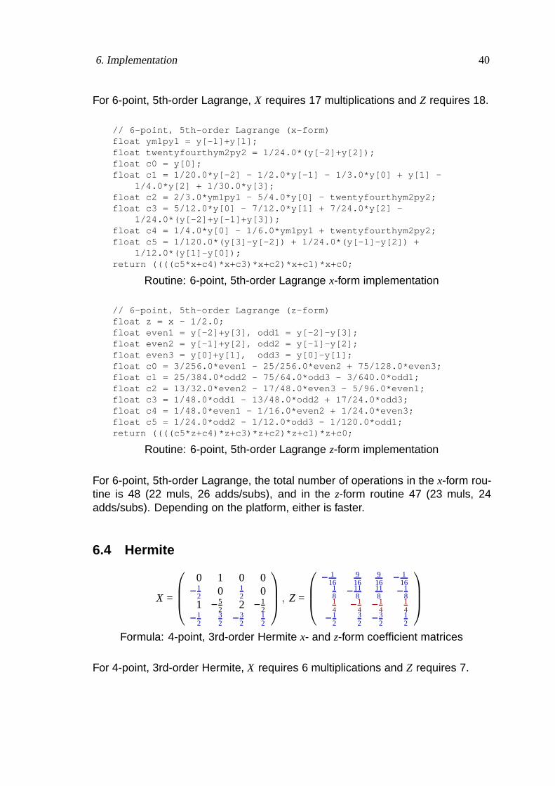
6. Implementation 40
For 6-point, 5th-order Lagrange, X requires 17 multiplications and Z requires 18.
// 6-point, 5th-order Lagrange (x-form)float ym1py1 = y[-1]+y[1];float twentyfourthym2py2 = 1/24.0*(y[-2]+y[2]);float c0 = y[0];float c1 = 1/20.0*y[-2] - 1/2.0*y[-1] - 1/3.0*y[0] + y[1] -
1/4.0*y[2] + 1/30.0*y[3];float c2 = 2/3.0*ym1py1 - 5/4.0*y[0] - twentyfourthym2py2;float c3 = 5/12.0*y[0] - 7/12.0*y[1] + 7/24.0*y[2] -
1/24.0*(y[-2]+y[-1]+y[3]);float c4 = 1/4.0*y[0] - 1/6.0*ym1py1 + twentyfourthym2py2;float c5 = 1/120.0*(y[3]-y[-2]) + 1/24.0*(y[-1]-y[2]) +
1/12.0*(y[1]-y[0]);return ((((c5*x+c4)*x+c3)*x+c2)*x+c1)*x+c0;
Routine: 6-point, 5th-order Lagrange x-form implementation
// 6-point, 5th-order Lagrange (z-form)float z = x - 1/2.0;float even1 = y[-2]+y[3], odd1 = y[-2]-y[3];float even2 = y[-1]+y[2], odd2 = y[-1]-y[2];float even3 = y[0]+y[1], odd3 = y[0]-y[1];float c0 = 3/256.0*even1 - 25/256.0*even2 + 75/128.0*even3;float c1 = 25/384.0*odd2 - 75/64.0*odd3 - 3/640.0*odd1;float c2 = 13/32.0*even2 - 17/48.0*even3 - 5/96.0*even1;float c3 = 1/48.0*odd1 - 13/48.0*odd2 + 17/24.0*odd3;float c4 = 1/48.0*even1 - 1/16.0*even2 + 1/24.0*even3;float c5 = 1/24.0*odd2 - 1/12.0*odd3 - 1/120.0*odd1;return ((((c5*z+c4)*z+c3)*z+c2)*z+c1)*z+c0;
Routine: 6-point, 5th-order Lagrange z-form implementation
For 6-point, 5th-order Lagrange, the total number of operations in the x-form rou-tine is 48 (22 muls, 26 adds/subs), and in the z-form routine 47 (23 muls, 24adds/subs). Depending on the platform, either is faster.
6.4 Hermite
X =
0 1 0 0−1
2 0 12 0
1 −52 2 −1
2−1
232 −3
212
, Z =
− 116
916
916 − 1
1618 −11
8118 −1
814 −1
4 −14
14
−12
32 −3
212
Formula: 4-point, 3rd-order Hermite x- and z-form coefficient matrices
For 4-point, 3rd-order Hermite, X requires 6 multiplications and Z requires 7.
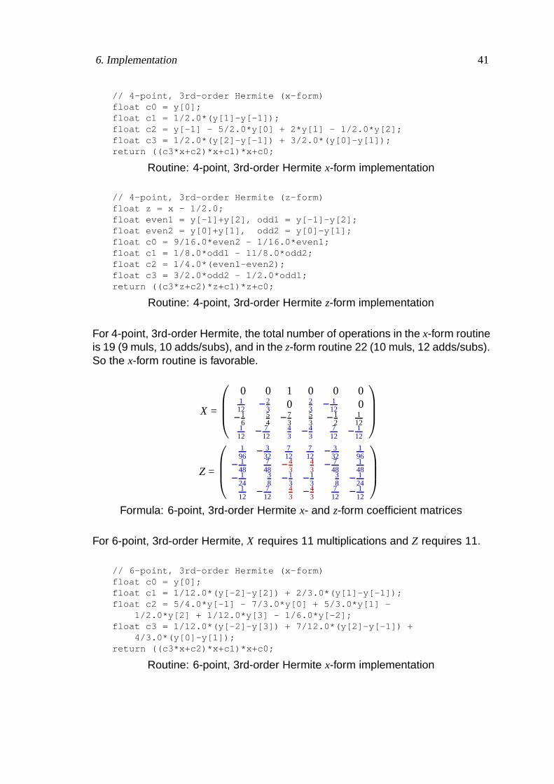
6. Implementation 41
// 4-point, 3rd-order Hermite (x-form)float c0 = y[0];float c1 = 1/2.0*(y[1]-y[-1]);float c2 = y[-1] - 5/2.0*y[0] + 2*y[1] - 1/2.0*y[2];float c3 = 1/2.0*(y[2]-y[-1]) + 3/2.0*(y[0]-y[1]);return ((c3*x+c2)*x+c1)*x+c0;
Routine: 4-point, 3rd-order Hermite x-form implementation
// 4-point, 3rd-order Hermite (z-form)float z = x - 1/2.0;float even1 = y[-1]+y[2], odd1 = y[-1]-y[2];float even2 = y[0]+y[1], odd2 = y[0]-y[1];float c0 = 9/16.0*even2 - 1/16.0*even1;float c1 = 1/8.0*odd1 - 11/8.0*odd2;float c2 = 1/4.0*(even1-even2);float c3 = 3/2.0*odd2 - 1/2.0*odd1;return ((c3*z+c2)*z+c1)*z+c0;
Routine: 4-point, 3rd-order Hermite z-form implementation
For 4-point, 3rd-order Hermite, the total number of operations in the x-form routineis 19 (9 muls, 10 adds/subs), and in the z-form routine 22 (10 muls, 12 adds/subs).So the x-form routine is favorable.
X =
0 0 1 0 0 01
12 −23 0 2
3 − 112 0
−16
54 −7
353 −1
21
121
12 − 712
43 −4
37
12 − 112
Z =
196 − 3
32712
712 − 3
32196
− 148
748 −4
343 − 7
48148
− 124
38 −1
3 −13
38 − 1
24112 − 7
1243 −4
3712 − 1
12
Formula: 6-point, 3rd-order Hermite x- and z-form coefficient matrices
For 6-point, 3rd-order Hermite, X requires 11 multiplications and Z requires 11.
// 6-point, 3rd-order Hermite (x-form)float c0 = y[0];float c1 = 1/12.0*(y[-2]-y[2]) + 2/3.0*(y[1]-y[-1]);float c2 = 5/4.0*y[-1] - 7/3.0*y[0] + 5/3.0*y[1] -
1/2.0*y[2] + 1/12.0*y[3] - 1/6.0*y[-2];float c3 = 1/12.0*(y[-2]-y[3]) + 7/12.0*(y[2]-y[-1]) +
4/3.0*(y[0]-y[1]);return ((c3*x+c2)*x+c1)*x+c0;
Routine: 6-point, 3rd-order Hermite x-form implementation
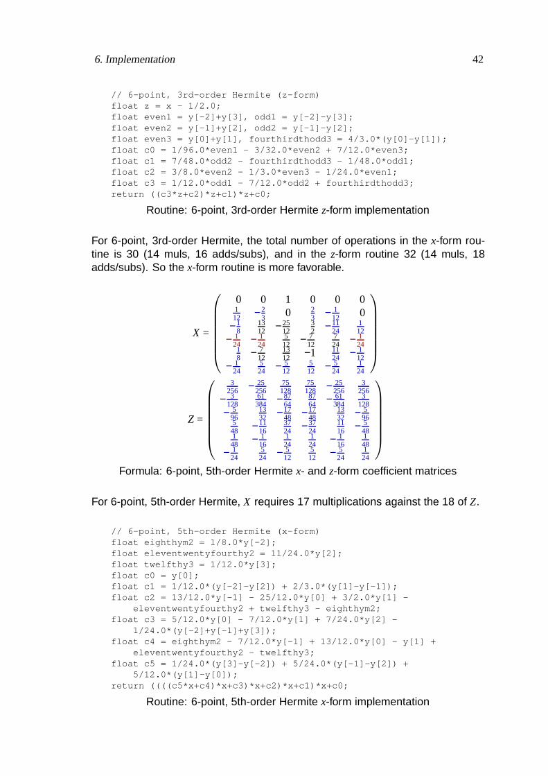
6. Implementation 42
// 6-point, 3rd-order Hermite (z-form)float z = x - 1/2.0;float even1 = y[-2]+y[3], odd1 = y[-2]-y[3];float even2 = y[-1]+y[2], odd2 = y[-1]-y[2];float even3 = y[0]+y[1], fourthirdthodd3 = 4/3.0*(y[0]-y[1]);float c0 = 1/96.0*even1 - 3/32.0*even2 + 7/12.0*even3;float c1 = 7/48.0*odd2 - fourthirdthodd3 - 1/48.0*odd1;float c2 = 3/8.0*even2 - 1/3.0*even3 - 1/24.0*even1;float c3 = 1/12.0*odd1 - 7/12.0*odd2 + fourthirdthodd3;return ((c3*z+c2)*z+c1)*z+c0;
Routine: 6-point, 3rd-order Hermite z-form implementation
For 6-point, 3rd-order Hermite, the total number of operations in the x-form rou-tine is 30 (14 muls, 16 adds/subs), and in the z-form routine 32 (14 muls, 18adds/subs). So the x-form routine is more favorable.
X =
0 0 1 0 0 0112 −2
3 0 23 − 1
12 0−1
81312 −25
1232 −11
24112
− 124 − 1
24512 − 7
12724 − 1
2418 − 7
121312 −1 11
24 − 112
− 124
524 − 5
12512 − 5
24124
Z =
3256 − 25
25675
12875
128 − 25256
3256
− 3128
61384 −87
648764 − 61
3843
128− 5
961332 −17
48 −1748
1332 − 5
965
48 −1116
3724 −37
241116 − 5
481
48 − 116
124
124 − 1
16148
− 124
524 − 5
125
12 − 524
124
Formula: 6-point, 5th-order Hermite x- and z-form coefficient matrices
For 6-point, 5th-order Hermite, X requires 17 multiplications against the 18 of Z.
// 6-point, 5th-order Hermite (x-form)float eighthym2 = 1/8.0*y[-2];float eleventwentyfourthy2 = 11/24.0*y[2];float twelfthy3 = 1/12.0*y[3];float c0 = y[0];float c1 = 1/12.0*(y[-2]-y[2]) + 2/3.0*(y[1]-y[-1]);float c2 = 13/12.0*y[-1] - 25/12.0*y[0] + 3/2.0*y[1] -
eleventwentyfourthy2 + twelfthy3 - eighthym2;float c3 = 5/12.0*y[0] - 7/12.0*y[1] + 7/24.0*y[2] -
1/24.0*(y[-2]+y[-1]+y[3]);float c4 = eighthym2 - 7/12.0*y[-1] + 13/12.0*y[0] - y[1] +
eleventwentyfourthy2 - twelfthy3;float c5 = 1/24.0*(y[3]-y[-2]) + 5/24.0*(y[-1]-y[2]) +
5/12.0*(y[1]-y[0]);return ((((c5*x+c4)*x+c3)*x+c2)*x+c1)*x+c0;
Routine: 6-point, 5th-order Hermite x-form implementation
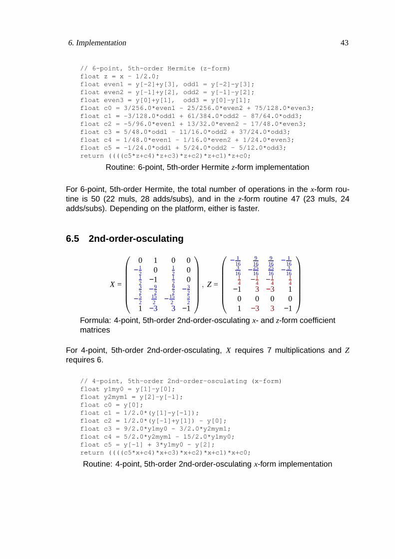
6. Implementation 43
// 6-point, 5th-order Hermite (z-form)float z = x - 1/2.0;float even1 = y[-2]+y[3], odd1 = y[-2]-y[3];float even2 = y[-1]+y[2], odd2 = y[-1]-y[2];float even3 = y[0]+y[1], odd3 = y[0]-y[1];float c0 = 3/256.0*even1 - 25/256.0*even2 + 75/128.0*even3;float c1 = -3/128.0*odd1 + 61/384.0*odd2 - 87/64.0*odd3;float c2 = -5/96.0*even1 + 13/32.0*even2 - 17/48.0*even3;float c3 = 5/48.0*odd1 - 11/16.0*odd2 + 37/24.0*odd3;float c4 = 1/48.0*even1 - 1/16.0*even2 + 1/24.0*even3;float c5 = -1/24.0*odd1 + 5/24.0*odd2 - 5/12.0*odd3;return ((((c5*z+c4)*z+c3)*z+c2)*z+c1)*z+c0;
Routine: 6-point, 5th-order Hermite z-form implementation
For 6-point, 5th-order Hermite, the total number of operations in the x-form rou-tine is 50 (22 muls, 28 adds/subs), and in the z-form routine 47 (23 muls, 24adds/subs). Depending on the platform, either is faster.
6.5 2nd-order-osculating
X =
0 1 0 0−1
2 0 12 0
12 −1 1
2 032 −9
292 −3
2−5
2152 −15
252
1 −3 3 −1
, Z =
− 116
916
916 − 1
16316 −25
162516 − 3
1614 −1
4 −14
14
−1 3 −3 10 0 0 01 −3 3 −1
Formula: 4-point, 5th-order 2nd-order-osculating x- and z-form coefficientmatrices
For 4-point, 5th-order 2nd-order-osculating, X requires 7 multiplications and Zrequires 6.
// 4-point, 5th-order 2nd-order-osculating (x-form)float y1my0 = y[1]-y[0];float y2mym1 = y[2]-y[-1];float c0 = y[0];float c1 = 1/2.0*(y[1]-y[-1]);float c2 = 1/2.0*(y[-1]+y[1]) - y[0];float c3 = 9/2.0*y1my0 - 3/2.0*y2mym1;float c4 = 5/2.0*y2mym1 - 15/2.0*y1my0;float c5 = y[-1] + 3*y1my0 - y[2];return ((((c5*x+c4)*x+c3)*x+c2)*x+c1)*x+c0;
Routine: 4-point, 5th-order 2nd-order-osculating x-form implementation
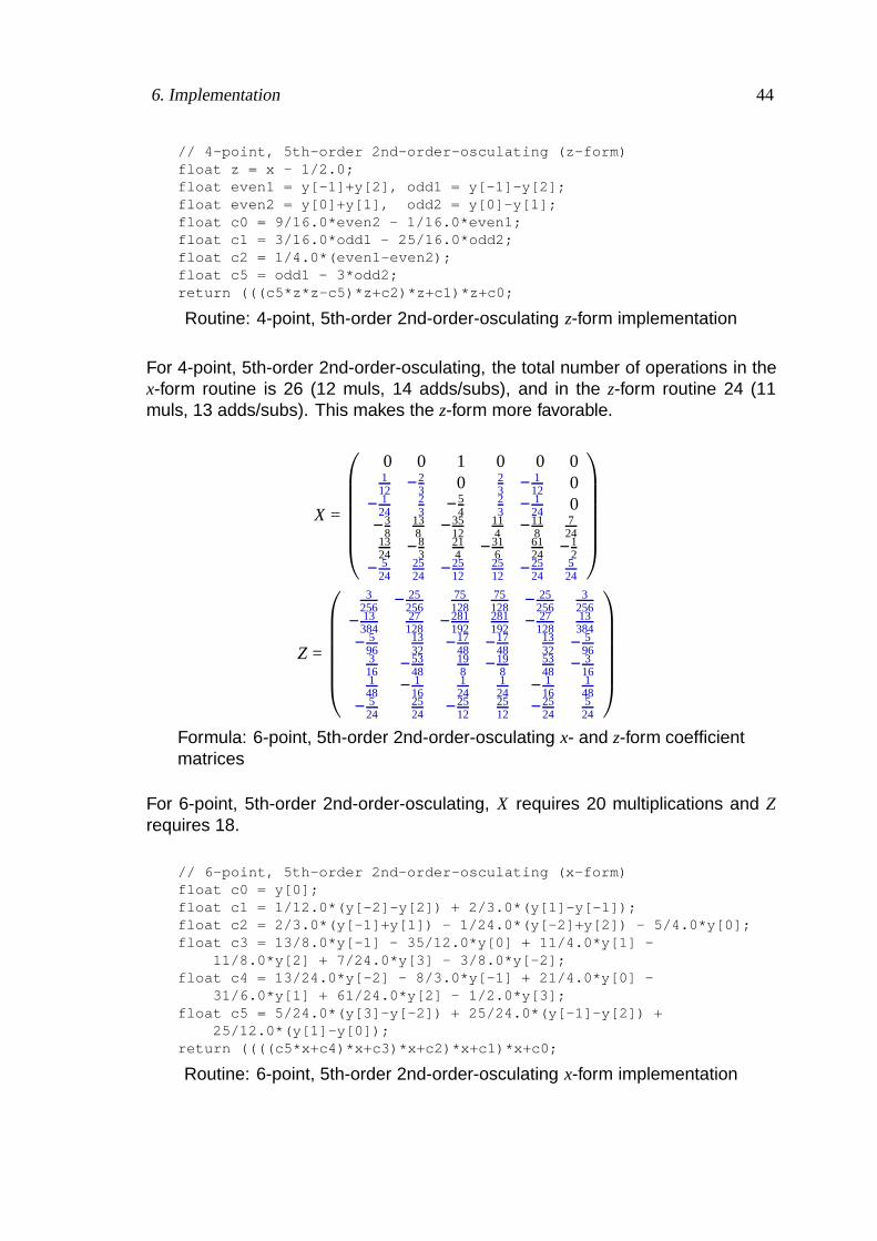
6. Implementation 44
// 4-point, 5th-order 2nd-order-osculating (z-form)float z = x - 1/2.0;float even1 = y[-1]+y[2], odd1 = y[-1]-y[2];float even2 = y[0]+y[1], odd2 = y[0]-y[1];float c0 = 9/16.0*even2 - 1/16.0*even1;float c1 = 3/16.0*odd1 - 25/16.0*odd2;float c2 = 1/4.0*(even1-even2);float c5 = odd1 - 3*odd2;return (((c5*z*z-c5)*z+c2)*z+c1)*z+c0;
Routine: 4-point, 5th-order 2nd-order-osculating z-form implementation
For 4-point, 5th-order 2nd-order-osculating, the total number of operations in thex-form routine is 26 (12 muls, 14 adds/subs), and in the z-form routine 24 (11muls, 13 adds/subs). This makes the z-form more favorable.
X =
0 0 1 0 0 0112 −2
3 0 23 − 1
12 0− 1
2423 −5
423 − 1
24 0−3
8138 −35
12114 −11
8724
1324 −8
3214 −31
66124 −1
2− 5
242524 −25
122512 −25
24524
Z =
3256 − 25
25675128
75128 − 25
2563
256− 13
38427
128 −281192
281192 − 27
12813
384− 5
961332 −17
48 −1748
1332 − 5
963
16 −5348
198 −19
85348 − 3
161
48 − 116
124
124 − 1
161
48− 5
242524 −25
122512 −25
245
24
Formula: 6-point, 5th-order 2nd-order-osculating x- and z-form coefficientmatrices
For 6-point, 5th-order 2nd-order-osculating, X requires 20 multiplications and Zrequires 18.
// 6-point, 5th-order 2nd-order-osculating (x-form)float c0 = y[0];float c1 = 1/12.0*(y[-2]-y[2]) + 2/3.0*(y[1]-y[-1]);float c2 = 2/3.0*(y[-1]+y[1]) - 1/24.0*(y[-2]+y[2]) - 5/4.0*y[0];float c3 = 13/8.0*y[-1] - 35/12.0*y[0] + 11/4.0*y[1] -
11/8.0*y[2] + 7/24.0*y[3] - 3/8.0*y[-2];float c4 = 13/24.0*y[-2] - 8/3.0*y[-1] + 21/4.0*y[0] -
31/6.0*y[1] + 61/24.0*y[2] - 1/2.0*y[3];float c5 = 5/24.0*(y[3]-y[-2]) + 25/24.0*(y[-1]-y[2]) +
25/12.0*(y[1]-y[0]);return ((((c5*x+c4)*x+c3)*x+c2)*x+c1)*x+c0;
Routine: 6-point, 5th-order 2nd-order-osculating x-form implementation
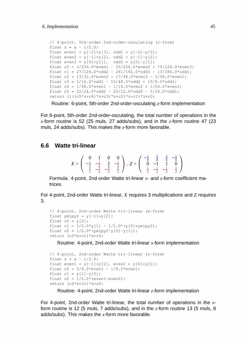
6. Implementation 45
// 6-point, 5th-order 2nd-order-osculating (z-form)float z = x - 1/2.0;float even1 = y[-2]+y[3], odd1 = y[-2]-y[3];float even2 = y[-1]+y[2], odd2 = y[-1]-y[2];float even3 = y[0]+y[1], odd3 = y[0]-y[1];float c0 = 3/256.0*even1 - 25/256.0*even2 + 75/128.0*even3;float c1 = 27/128.0*odd2 - 281/192.0*odd3 - 13/384.0*odd1;float c2 = 13/32.0*even2 - 17/48.0*even3 - 5/96.0*even1;float c3 = 3/16.0*odd1 - 53/48.0*odd2 + 19/8.0*odd3;float c4 = 1/48.0*even1 - 1/16.0*even2 + 1/24.0*even3;float c5 = 25/24.0*odd2 - 25/12.0*odd3 - 5/24.0*odd1;return ((((c5*z+c4)*z+c3)*z+c2)*z+c1)*z+c0;
Routine: 6-point, 5th-order 2nd-order-osculating z-form implementation
For 6-point, 5th-order 2nd-order-osculating, the total number of operations in thex-form routine is 52 (25 muls, 27 adds/subs), and in the z-form routine 47 (23muls, 24 adds/subs). This makes the z-form more favorable.
6.6 Watte tri-linear
X =
0 1 0 0
−12 −1
232 −1
212 −1
2 −12
12
, Z =
−1
858
58 −1
80 −1 1 012 −1
2 −12
12
Formula: 4-point, 2nd-order Watte tri-linear x- and z-form coefficient ma-trices
For 4-point, 2nd-order Watte tri-linear, X requires 3 multiplications and Z requires3.
// 4-point, 2nd-order Watte tri-linear (x-form)float ym1py2 = y[-1]+y[2];float c0 = y[0];float c1 = 3/2.0*y[1] - 1/2.0*(y[0]+ym1py2);float c2 = 1/2.0*(ym1py2-y[0]-y[1]);return (c2*x+c1)*x+c0;
Routine: 4-point, 2nd-order Watte tri-linear x-form implementation
// 4-point, 2nd-order Watte tri-linear (z-form)float z = x - 1/2.0;float even1 = y[-1]+y[2], even2 = y[0]+y[1];float c0 = 5/8.0*even2 - 1/8.0*even1;float c1 = y[1]-y[0];float c2 = 1/2.0*(even1-even2);return (c2*z+c1)*z+c0;
Routine: 4-point, 2nd-order Watte tri-linear z-form implementation
For 4-point, 2nd-order Watte tri-linear, the total number of operations in the x-form routine is 12 (5 muls, 7 adds/subs), and in the z-form routine 13 (5 muls, 8adds/subs). This makes the x-form more favorable.
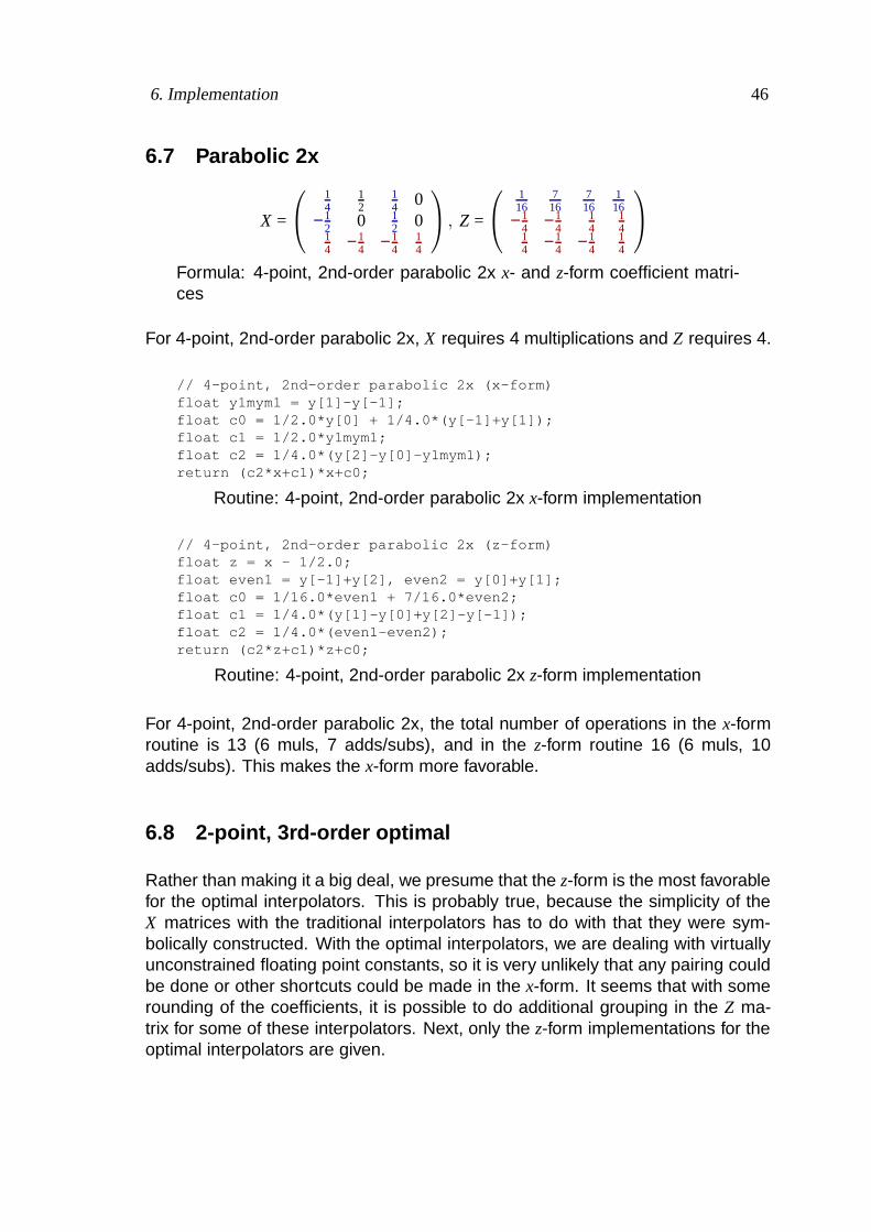
6. Implementation 46
6.7 Parabolic 2x
X =
14
12
14 0
−12 0 1
2 014 −1
4 −14
14
, Z =
116
716
716
116
−14 −1
414
14
14 −1
4 −14
14
Formula: 4-point, 2nd-order parabolic 2x x- and z-form coefficient matri-ces
For 4-point, 2nd-order parabolic 2x, X requires 4 multiplications and Z requires 4.
// 4-point, 2nd-order parabolic 2x (x-form)float y1mym1 = y[1]-y[-1];float c0 = 1/2.0*y[0] + 1/4.0*(y[-1]+y[1]);float c1 = 1/2.0*y1mym1;float c2 = 1/4.0*(y[2]-y[0]-y1mym1);return (c2*x+c1)*x+c0;
Routine: 4-point, 2nd-order parabolic 2x x-form implementation
// 4-point, 2nd-order parabolic 2x (z-form)float z = x - 1/2.0;float even1 = y[-1]+y[2], even2 = y[0]+y[1];float c0 = 1/16.0*even1 + 7/16.0*even2;float c1 = 1/4.0*(y[1]-y[0]+y[2]-y[-1]);float c2 = 1/4.0*(even1-even2);return (c2*z+c1)*z+c0;
Routine: 4-point, 2nd-order parabolic 2x z-form implementation
For 4-point, 2nd-order parabolic 2x, the total number of operations in the x-formroutine is 13 (6 muls, 7 adds/subs), and in the z-form routine 16 (6 muls, 10adds/subs). This makes the x-form more favorable.
6.8 2-point, 3rd-order optimal
Rather than making it a big deal, we presume that the z-form is the most favorablefor the optimal interpolators. This is probably true, because the simplicity of theX matrices with the traditional interpolators has to do with that they were sym-bolically constructed. With the optimal interpolators, we are dealing with virtuallyunconstrained floating point constants, so it is very unlikely that any pairing couldbe done or other shortcuts could be made in the x-form. It seems that with somerounding of the coefficients, it is possible to do additional grouping in the Z ma-trix for some of these interpolators. Next, only the z-form implementations for theoptimal interpolators are given.
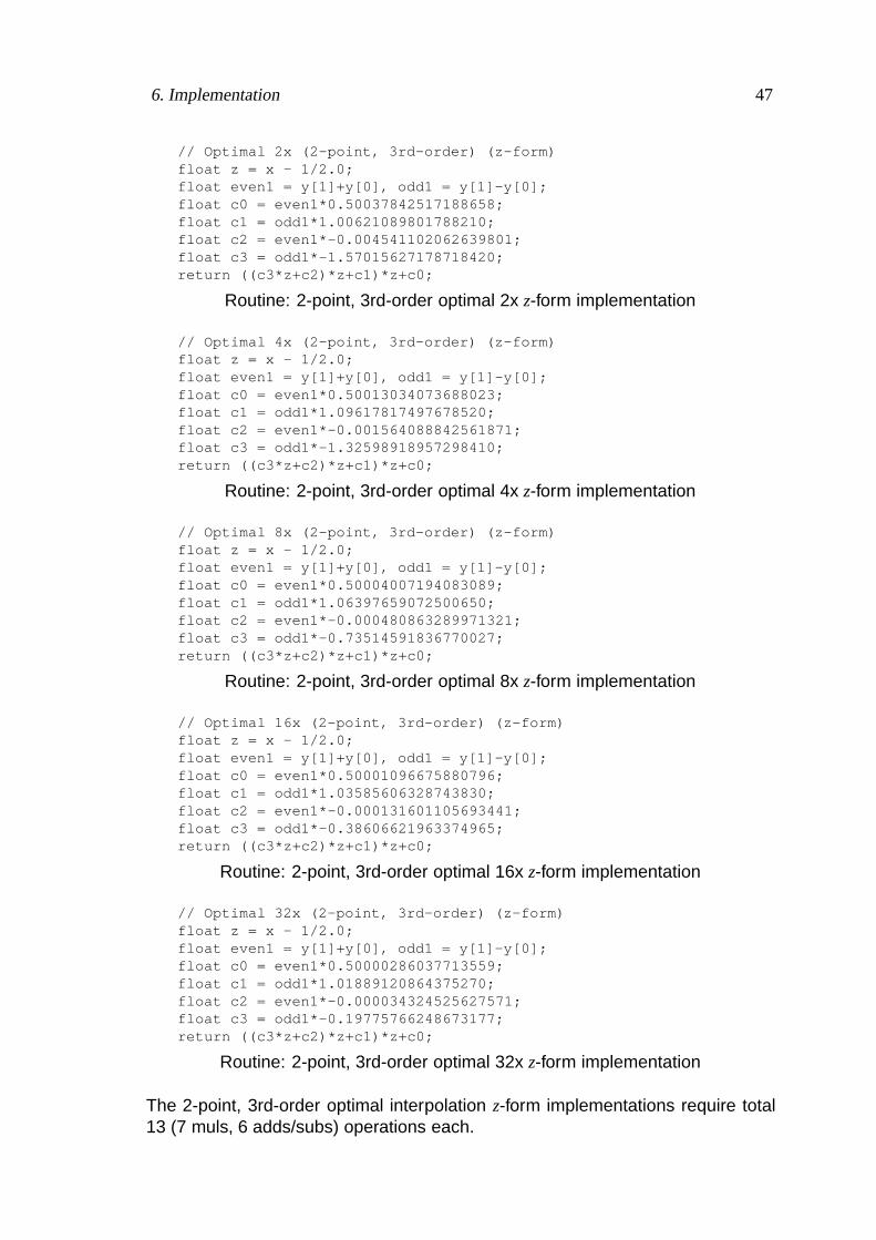
6. Implementation 47
// Optimal 2x (2-point, 3rd-order) (z-form)float z = x - 1/2.0;float even1 = y[1]+y[0], odd1 = y[1]-y[0];float c0 = even1*0.50037842517188658;float c1 = odd1*1.00621089801788210;float c2 = even1*-0.004541102062639801;float c3 = odd1*-1.57015627178718420;return ((c3*z+c2)*z+c1)*z+c0;
Routine: 2-point, 3rd-order optimal 2x z-form implementation
// Optimal 4x (2-point, 3rd-order) (z-form)float z = x - 1/2.0;float even1 = y[1]+y[0], odd1 = y[1]-y[0];float c0 = even1*0.50013034073688023;float c1 = odd1*1.09617817497678520;float c2 = even1*-0.001564088842561871;float c3 = odd1*-1.32598918957298410;return ((c3*z+c2)*z+c1)*z+c0;
Routine: 2-point, 3rd-order optimal 4x z-form implementation
// Optimal 8x (2-point, 3rd-order) (z-form)float z = x - 1/2.0;float even1 = y[1]+y[0], odd1 = y[1]-y[0];float c0 = even1*0.50004007194083089;float c1 = odd1*1.06397659072500650;float c2 = even1*-0.000480863289971321;float c3 = odd1*-0.73514591836770027;return ((c3*z+c2)*z+c1)*z+c0;
Routine: 2-point, 3rd-order optimal 8x z-form implementation
// Optimal 16x (2-point, 3rd-order) (z-form)float z = x - 1/2.0;float even1 = y[1]+y[0], odd1 = y[1]-y[0];float c0 = even1*0.50001096675880796;float c1 = odd1*1.03585606328743830;float c2 = even1*-0.000131601105693441;float c3 = odd1*-0.38606621963374965;return ((c3*z+c2)*z+c1)*z+c0;
Routine: 2-point, 3rd-order optimal 16x z-form implementation
// Optimal 32x (2-point, 3rd-order) (z-form)float z = x - 1/2.0;float even1 = y[1]+y[0], odd1 = y[1]-y[0];float c0 = even1*0.50000286037713559;float c1 = odd1*1.01889120864375270;float c2 = even1*-0.000034324525627571;float c3 = odd1*-0.19775766248673177;return ((c3*z+c2)*z+c1)*z+c0;
Routine: 2-point, 3rd-order optimal 32x z-form implementation
The 2-point, 3rd-order optimal interpolation z-form implementations require total13 (7 muls, 6 adds/subs) operations each.
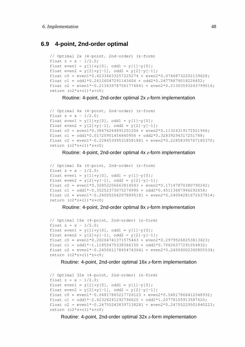
6. Implementation 48
6.9 4-point, 2nd-order optimal
// Optimal 2x (4-point, 2nd-order) (z-form)float z = x - 1/2.0;float even1 = y[1]+y[0], odd1 = y[1]-y[0];float even2 = y[2]+y[-1], odd2 = y[2]-y[-1];float c0 = even1*0.42334633257225274 + even2*0.07668732202139628;float c1 = odd1*0.26126047291143606 + odd2*0.24778879018226652;float c2 = even1*-0.213439787561776841 + even2*0.21303593243799016;return (c2*z+c1)*z+c0;
Routine: 4-point, 2nd-order optimal 2x z-form implementation
// Optimal 4x (4-point, 2nd-order) (z-form)float z = x - 1/2.0;float even1 = y[1]+y[0], odd1 = y[1]-y[0];float even2 = y[2]+y[-1], odd2 = y[2]-y[-1];float c0 = even1*0.38676264891201206 + even2*0.11324319172521946;float c1 = odd1*0.01720901456660906 + odd2*0.32839294317251788;float c2 = even1*-0.228653995318581881 + even2*0.22858390767180370;return (c2*z+c1)*z+c0;
Routine: 4-point, 2nd-order optimal 4x z-form implementation
// Optimal 8x (4-point, 2nd-order) (z-form)float z = x - 1/2.0;float even1 = y[1]+y[0], odd1 = y[1]-y[0];float even2 = y[2]+y[-1], odd2 = y[2]-y[-1];float c0 = even1*0.32852206663814043 + even2*0.17147870380790242;float c1 = odd1*-0.35252373075274990 + odd2*0.45113687946292658;float c2 = even1*-0.240052062078895181 + even2*0.24004281672637814;return (c2*z+c1)*z+c0;
Routine: 4-point, 2nd-order optimal 8x z-form implementation
// Optimal 16x (4-point, 2nd-order) (z-form)float z = x - 1/2.0;float even1 = y[1]+y[0], odd1 = y[1]-y[0];float even2 = y[2]+y[-1], odd2 = y[2]-y[-1];float c0 = even1*0.20204741371575463 + even2*0.29795268253813623;float c1 = odd1*-1.11855475338366150 + odd2*0.70626377291054832;float c2 = even1*-0.245061178654743641 + even2*0.24506002360805534;return (c2*z+c1)*z+c0;
Routine: 4-point, 2nd-order optimal 16x z-form implementation
// Optimal 32x (4-point, 2nd-order) (z-form)float z = x - 1/2.0;float even1 = y[1]+y[0], odd1 = y[1]-y[0];float even2 = y[2]+y[-1], odd2 = y[2]-y[-1];float c0 = even1*-0.04817865217726123 + even2*0.54817866412548932;float c1 = odd1*-2.62328241292796620 + odd2*1.20778105913587620;float c2 = even1*-0.247552438397138281 + even2*0.24755229501840223;return (c2*z+c1)*z+c0;
Routine: 4-point, 2nd-order optimal 32x z-form implementation
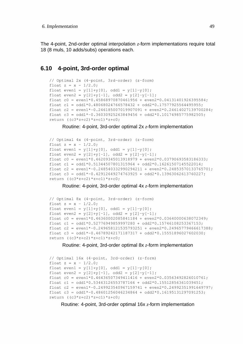
6. Implementation 49
The 4-point, 2nd-order optimal interpolation z-form implementations require total18 (8 muls, 10 adds/subs) operations each.
6.10 4-point, 3rd-order optimal
// Optimal 2x (4-point, 3rd-order) (z-form)float z = x - 1/2.0;float even1 = y[1]+y[0], odd1 = y[1]-y[0];float even2 = y[2]+y[-1], odd2 = y[2]-y[-1];float c0 = even1*0.45868970870461956 + even2*0.04131401926395584;float c1 = odd1*0.48068024766578432 + odd2*0.17577925564495955;float c2 = even1*-0.246185007019907091 + even2*0.24614027139700284;float c3 = odd1*-0.36030925263849456 + odd2*0.10174985775982505;return ((c3*z+c2)*z+c1)*z+c0;
Routine: 4-point, 3rd-order optimal 2x z-form implementation
// Optimal 4x (4-point, 3rd-order) (z-form)float z = x - 1/2.0;float even1 = y[1]+y[0], odd1 = y[1]-y[0];float even2 = y[2]+y[-1], odd2 = y[2]-y[-1];float c0 = even1*0.46209345013918979 + even2*0.03790693583186333;float c1 = odd1*0.51344507801315964 + odd2*0.16261507145522014;float c2 = even1*-0.248540332990294211 + even2*0.24853570133765701;float c3 = odd1*-0.42912649274763925 + odd2*0.13963062613760227;return ((c3*z+c2)*z+c1)*z+c0;
Routine: 4-point, 3rd-order optimal 4x z-form implementation
// Optimal 8x (4-point, 3rd-order) (z-form)float z = x - 1/2.0;float even1 = y[1]+y[0], odd1 = y[1]-y[0];float even2 = y[2]+y[-1], odd2 = y[2]-y[-1];float c0 = even1*0.46360002085841184 + even2*0.03640000638072349;float c1 = odd1*0.52776949859997280 + odd2*0.15746108253367153;float c2 = even1*-0.249658121535793251 + even2*0.24965779466617388;float c3 = odd1*-0.46789242171187317 + odd2*0.15551896027602030;return ((c3*z+c2)*z+c1)*z+c0;
Routine: 4-point, 3rd-order optimal 8x z-form implementation
// Optimal 16x (4-point, 3rd-order) (z-form)float z = x - 1/2.0;float even1 = y[1]+y[0], odd1 = y[1]-y[0];float even2 = y[2]+y[-1], odd2 = y[2]-y[-1];float c0 = even1*0.46436507349411416 + even2*0.03563492826010761;float c1 = odd1*0.53463126553787166 + odd2*0.15512856361039451;float c2 = even1*-0.249923540967159741 + even2*0.24992351991649797;float c3 = odd1*-0.48601256046234864 + odd2*0.16195131297091253;return ((c3*z+c2)*z+c1)*z+c0;
Routine: 4-point, 3rd-order optimal 16x z-form implementation
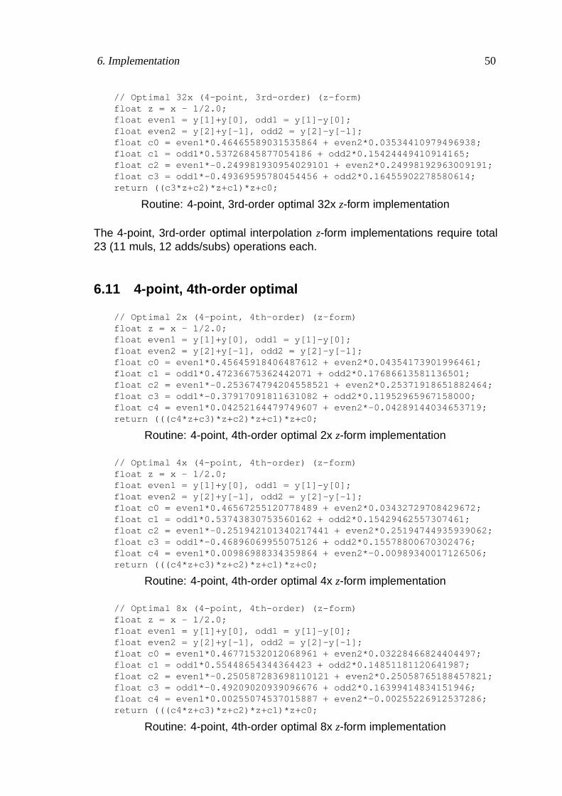
6. Implementation 50
// Optimal 32x (4-point, 3rd-order) (z-form)float z = x - 1/2.0;float even1 = y[1]+y[0], odd1 = y[1]-y[0];float even2 = y[2]+y[-1], odd2 = y[2]-y[-1];float c0 = even1*0.46465589031535864 + even2*0.03534410979496938;float c1 = odd1*0.53726845877054186 + odd2*0.15424449410914165;float c2 = even1*-0.249981930954029101 + even2*0.24998192963009191;float c3 = odd1*-0.49369595780454456 + odd2*0.16455902278580614;return ((c3*z+c2)*z+c1)*z+c0;
Routine: 4-point, 3rd-order optimal 32x z-form implementation
The 4-point, 3rd-order optimal interpolation z-form implementations require total23 (11 muls, 12 adds/subs) operations each.
6.11 4-point, 4th-order optimal
// Optimal 2x (4-point, 4th-order) (z-form)float z = x - 1/2.0;float even1 = y[1]+y[0], odd1 = y[1]-y[0];float even2 = y[2]+y[-1], odd2 = y[2]-y[-1];float c0 = even1*0.45645918406487612 + even2*0.04354173901996461;float c1 = odd1*0.47236675362442071 + odd2*0.17686613581136501;float c2 = even1*-0.253674794204558521 + even2*0.25371918651882464;float c3 = odd1*-0.37917091811631082 + odd2*0.11952965967158000;float c4 = even1*0.04252164479749607 + even2*-0.04289144034653719;return (((c4*z+c3)*z+c2)*z+c1)*z+c0;
Routine: 4-point, 4th-order optimal 2x z-form implementation
// Optimal 4x (4-point, 4th-order) (z-form)float z = x - 1/2.0;float even1 = y[1]+y[0], odd1 = y[1]-y[0];float even2 = y[2]+y[-1], odd2 = y[2]-y[-1];float c0 = even1*0.46567255120778489 + even2*0.03432729708429672;float c1 = odd1*0.53743830753560162 + odd2*0.15429462557307461;float c2 = even1*-0.251942101340217441 + even2*0.25194744935939062;float c3 = odd1*-0.46896069955075126 + odd2*0.15578800670302476;float c4 = even1*0.00986988334359864 + even2*-0.00989340017126506;return (((c4*z+c3)*z+c2)*z+c1)*z+c0;
Routine: 4-point, 4th-order optimal 4x z-form implementation
// Optimal 8x (4-point, 4th-order) (z-form)float z = x - 1/2.0;float even1 = y[1]+y[0], odd1 = y[1]-y[0];float even2 = y[2]+y[-1], odd2 = y[2]-y[-1];float c0 = even1*0.46771532012068961 + even2*0.03228466824404497;float c1 = odd1*0.55448654344364423 + odd2*0.14851181120641987;float c2 = even1*-0.250587283698110121 + even2*0.25058765188457821;float c3 = odd1*-0.49209020939096676 + odd2*0.16399414834151946;float c4 = even1*0.00255074537015887 + even2*-0.00255226912537286;return (((c4*z+c3)*z+c2)*z+c1)*z+c0;
Routine: 4-point, 4th-order optimal 8x z-form implementation
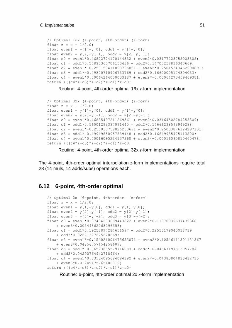
6. Implementation 51
// Optimal 16x (4-point, 4th-order) (z-form)float z = x - 1/2.0;float even1 = y[1]+y[0], odd1 = y[1]-y[0];float even2 = y[2]+y[-1], odd2 = y[2]-y[-1];float c0 = even1*0.46822774170144532 + even2*0.03177225758005808;float c1 = odd1*0.55890365706150436 + odd2*0.14703258836343669;float c2 = even1*-0.250153411893796031 + even2*0.25015343462990891;float c3 = odd1*-0.49800710906733769 + odd2*0.16600005174304033;float c4 = even1*0.00064264050033187 + even2*-0.00064273459469381;return (((c4*z+c3)*z+c2)*z+c1)*z+c0;
Routine: 4-point, 4th-order optimal 16x z-form implementation
// Optimal 32x (4-point, 4th-order) (z-form)float z = x - 1/2.0;float even1 = y[1]+y[0], odd1 = y[1]-y[0];float even2 = y[2]+y[-1], odd2 = y[2]-y[-1];float c0 = even1*0.46835497211269561 + even2*0.03164502784253309;float c1 = odd1*0.56001293337091440 + odd2*0.14666238593949288;float c2 = even1*-0.250038759826233691 + even2*0.25003876124297131;float c3 = odd1*-0.49949850957839148 + odd2*0.16649935475113800;float c4 = even1*0.00016095224137360 + even2*-0.00016095810460478;return (((c4*z+c3)*z+c2)*z+c1)*z+c0;
Routine: 4-point, 4th-order optimal 32x z-form implementation
The 4-point, 4th-order optimal interpolation z-form implementations require total28 (14 muls, 14 adds/subs) operations each.
6.12 6-point, 4th-order optimal
// Optimal 2x (6-point, 4th-order) (z-form)float z = x - 1/2.0;float even1 = y[1]+y[0], odd1 = y[1]-y[0];float even2 = y[2]+y[-1], odd2 = y[2]-y[-1];float even3 = y[3]+y[-2], odd3 = y[3]-y[-2];float c0 = even1*0.37484203669443822 + even2*0.11970939637439368
+ even3*0.00544862268096358;float c1 = odd1*0.19253897284651597 + odd2*0.22555179040018719
+ odd3*0.02621377625620669;float c2 = even1*-0.154026006475653071 + even2*0.10546111301131367
+ even3*0.04856757454258609;float c3 = odd1*-0.06523685579716083 + odd2*-0.04867197815057284
+ odd3*0.04200764942718964;float c4 = even1*0.03134095684084392 + even2*-0.04385804833432710
+ even3*0.01249475765486819;return (((c4*z+c3)*z+c2)*z+c1)*z+c0;
Routine: 6-point, 4th-order optimal 2x z-form implementation
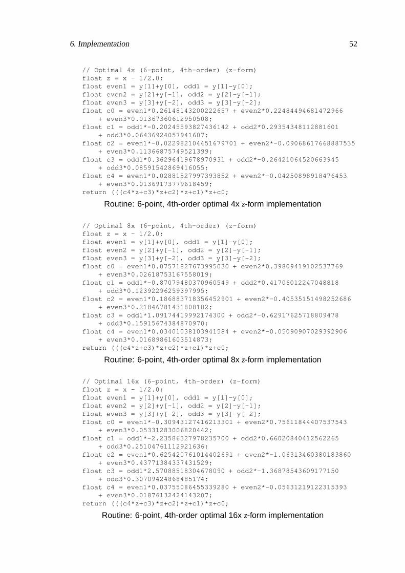
6. Implementation 52
// Optimal 4x (6-point, 4th-order) (z-form)float z = x - 1/2.0;float even1 = y[1]+y[0], odd1 = y[1]-y[0];float even2 = y[2]+y[-1], odd2 = y[2]-y[-1];float even3 = y[3]+y[-2], odd3 = y[3]-y[-2];float c0 = even1*0.26148143200222657 + even2*0.22484494681472966
+ even3*0.01367360612950508;float c1 = odd1*-0.20245593827436142 + odd2*0.29354348112881601
+ odd3*0.06436924057941607;float c2 = even1*-0.022982104451679701 + even2*-0.09068617668887535
+ even3*0.11366875749521399;float c3 = odd1*0.36296419678970931 + odd2*-0.26421064520663945
+ odd3*0.08591542869416055;float c4 = even1*0.02881527997393852 + even2*-0.04250898918476453
+ even3*0.01369173779618459;return (((c4*z+c3)*z+c2)*z+c1)*z+c0;
Routine: 6-point, 4th-order optimal 4x z-form implementation
// Optimal 8x (6-point, 4th-order) (z-form)float z = x - 1/2.0;float even1 = y[1]+y[0], odd1 = y[1]-y[0];float even2 = y[2]+y[-1], odd2 = y[2]-y[-1];float even3 = y[3]+y[-2], odd3 = y[3]-y[-2];float c0 = even1*0.07571827673995030 + even2*0.39809419102537769
+ even3*0.02618753167558019;float c1 = odd1*-0.87079480370960549 + odd2*0.41706012247048818
+ odd3*0.12392296259397995;float c2 = even1*0.186883718356452901 + even2*-0.40535151498252686
+ even3*0.21846781431808182;float c3 = odd1*1.09174419992174300 + odd2*-0.62917625718809478
+ odd3*0.15915674384870970;float c4 = even1*0.03401038103941584 + even2*-0.05090907029392906
+ even3*0.01689861603514873;return (((c4*z+c3)*z+c2)*z+c1)*z+c0;
Routine: 6-point, 4th-order optimal 8x z-form implementation
// Optimal 16x (6-point, 4th-order) (z-form)float z = x - 1/2.0;float even1 = y[1]+y[0], odd1 = y[1]-y[0];float even2 = y[2]+y[-1], odd2 = y[2]-y[-1];float even3 = y[3]+y[-2], odd3 = y[3]-y[-2];float c0 = even1*-0.30943127416213301 + even2*0.75611844407537543
+ even3*0.05331283006820442;float c1 = odd1*-2.23586327978235700 + odd2*0.66020840412562265
+ odd3*0.25104761112921636;float c2 = even1*0.625420761014402691 + even2*-1.06313460380183860
+ even3*0.43771384337431529;float c3 = odd1*2.57088518304678090 + odd2*-1.36878543609177150
+ odd3*0.30709424868485174;float c4 = even1*0.03755086455339280 + even2*-0.05631219122315393
+ even3*0.01876132424143207;return (((c4*z+c3)*z+c2)*z+c1)*z+c0;
Routine: 6-point, 4th-order optimal 16x z-form implementation
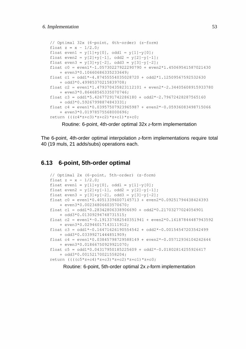
6. Implementation 53
// Optimal 32x (6-point, 4th-order) (z-form)float z = x - 1/2.0;float even1 = y[1]+y[0], odd1 = y[1]-y[0];float even2 = y[2]+y[-1], odd2 = y[2]-y[-1];float even3 = y[3]+y[-2], odd3 = y[3]-y[-2];float c0 = even1*-1.05730227922290790 + even2*1.45069541587021430
+ even3*0.10660686335233649;float c1 = odd1*-4.87455554035028720 + odd2*1.12509567592532630
+ odd3*0.49985370215839708;float c2 = even1*1.479370435823112101 + even2*-2.34405608915933780
+ even3*0.86468565335070746;float c3 = odd1*5.42677291742286180 + odd2*-2.79672428287565160
+ odd3*0.59267998874843331;float c4 = even1*0.03957507923965987 + even2*-0.05936083498715066
+ even3*0.01978575568000696;return (((c4*z+c3)*z+c2)*z+c1)*z+c0;
Routine: 6-point, 4th-order optimal 32x z-form implementation
The 6-point, 4th-order optimal interpolation z-form implementations require total40 (19 muls, 21 adds/subs) operations each.
6.13 6-point, 5th-order optimal
// Optimal 2x (6-point, 5th-order) (z-form)float z = x - 1/2.0;float even1 = y[1]+y[0], odd1 = y[1]-y[0];float even2 = y[2]+y[-1], odd2 = y[2]-y[-1];float even3 = y[3]+y[-2], odd3 = y[3]-y[-2];float c0 = even1*0.40513396007145713 + even2*0.09251794438424393
+ even3*0.00234806603570670;float c1 = odd1*0.28342806338906690 + odd2*0.21703277024054901
+ odd3*0.01309294748731515;float c2 = even1*-0.191337682540351941 + even2*0.16187844487943592
+ even3*0.02946017143111912;float c3 = odd1*-0.16471626190554542 + odd2*-0.00154547203542499
+ odd3*0.03399271444851909;float c4 = even1*0.03845798729588149 + even2*-0.05712936104242644
+ even3*0.01866750929921070;float c5 = odd1*0.04317950185225609 + odd2*-0.01802814255926417
+ odd3*0.00152170021558204;return ((((c5*z+c4)*z+c3)*z+c2)*z+c1)*z+c0;
Routine: 6-point, 5th-order optimal 2x z-form implementation
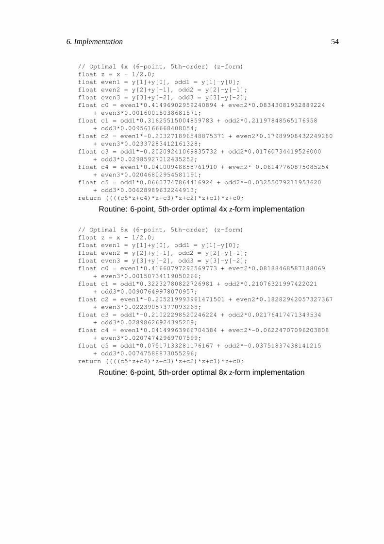
6. Implementation 54
// Optimal 4x (6-point, 5th-order) (z-form)float z = x - 1/2.0;float even1 = y[1]+y[0], odd1 = y[1]-y[0];float even2 = y[2]+y[-1], odd2 = y[2]-y[-1];float even3 = y[3]+y[-2], odd3 = y[3]-y[-2];float c0 = even1*0.41496902959240894 + even2*0.08343081932889224
+ even3*0.00160015038681571;float c1 = odd1*0.31625515004859783 + odd2*0.21197848565176958
+ odd3*0.00956166668408054;float c2 = even1*-0.203271896548875371 + even2*0.17989908432249280
+ even3*0.02337283412161328;float c3 = odd1*-0.20209241069835732 + odd2*0.01760734419526000
+ odd3*0.02985927012435252;float c4 = even1*0.04100948858761910 + even2*-0.06147760875085254
+ even3*0.02046802954581191;float c5 = odd1*0.06607747864416924 + odd2*-0.03255079211953620
+ odd3*0.00628989632244913;return ((((c5*z+c4)*z+c3)*z+c2)*z+c1)*z+c0;
Routine: 6-point, 5th-order optimal 4x z-form implementation
// Optimal 8x (6-point, 5th-order) (z-form)float z = x - 1/2.0;float even1 = y[1]+y[0], odd1 = y[1]-y[0];float even2 = y[2]+y[-1], odd2 = y[2]-y[-1];float even3 = y[3]+y[-2], odd3 = y[3]-y[-2];float c0 = even1*0.41660797292569773 + even2*0.08188468587188069
+ even3*0.00150734119050266;float c1 = odd1*0.32232780822726981 + odd2*0.21076321997422021
+ odd3*0.00907649978070957;float c2 = even1*-0.205219993961471501 + even2*0.18282942057327367
+ even3*0.02239057377093268;float c3 = odd1*-0.21022298520246224 + odd2*0.02176417471349534
+ odd3*0.02898626924395209;float c4 = even1*0.04149963966704384 + even2*-0.06224707096203808
+ even3*0.02074742969707599;float c5 = odd1*0.07517133281176167 + odd2*-0.03751837438141215
+ odd3*0.00747588873055296;return ((((c5*z+c4)*z+c3)*z+c2)*z+c1)*z+c0;
Routine: 6-point, 5th-order optimal 8x z-form implementation
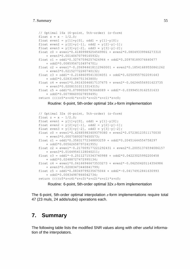
7. Summary 55
// Optimal 16x (6-point, 5th-order) (z-form)float z = x - 1/2.0;float even1 = y[1]+y[0], odd1 = y[1]-y[0];float even2 = y[2]+y[-1], odd2 = y[2]-y[-1];float even3 = y[3]+y[-2], odd3 = y[3]-y[-2];float c0 = even1*0.41809989254549901 + even2*0.08049339946273310
+ even3*0.00140670799165932;float c1 = odd1*0.32767596257424964 + odd2*0.20978189376640677
+ odd3*0.00859567104974701;float c2 = even1*-0.206944618112960001 + even2*0.18541689550861262
+ even3*0.02152772260740132;float c3 = odd1*-0.21686095413034051 + odd2*0.02509557922091643
+ odd3*0.02831484751363800;float c4 = even1*0.04163046817137675 + even2*-0.06244556931623735
+ even3*0.02081510113314315;float c5 = odd1*0.07990500783668089 + odd2*-0.03994519162531633
+ odd3*0.00798609327859495;return ((((c5*z+c4)*z+c3)*z+c2)*z+c1)*z+c0;
Routine: 6-point, 5th-order optimal 16x z-form implementation
// Optimal 32x (6-point, 5th-order) (z-form)float z = x - 1/2.0;float even1 = y[1]+y[0], odd1 = y[1]-y[0];float even2 = y[2]+y[-1], odd2 = y[2]-y[-1];float even3 = y[3]+y[-2], odd3 = y[3]-y[-2];float c0 = even1*0.42685983409379380 + even2*0.07238123511170030
+ even3*0.00075893079450573;float c1 = odd1*0.35831772348893259 + odd2*0.20451644554758297
+ odd3*0.00562658797241955;float c2 = even1*-0.217009177221292431 + even2*0.20051376594086157
+ even3*0.01649541128040211;float c3 = odd1*-0.25112715343740988 + odd2*0.04223025992200458
+ odd3*0.02488727472995134;float c4 = even1*0.04166946673533273 + even2*-0.06250420114356986
+ even3*0.02083473440841799;float c5 = odd1*0.08349799235675044 + odd2*-0.04174912841630993
+ odd3*0.00834987866042734;return ((((c5*z+c4)*z+c3)*z+c2)*z+c1)*z+c0;
Routine: 6-point, 5th-order optimal 32x z-form implementation
The 6-point, 5th-order optimal interpolation z-form implementations require total47 (23 muls, 24 adds/subs) operations each.
7. Summary
The following table lists the modified SNR values along with other useful informa-tion of the interpolators.
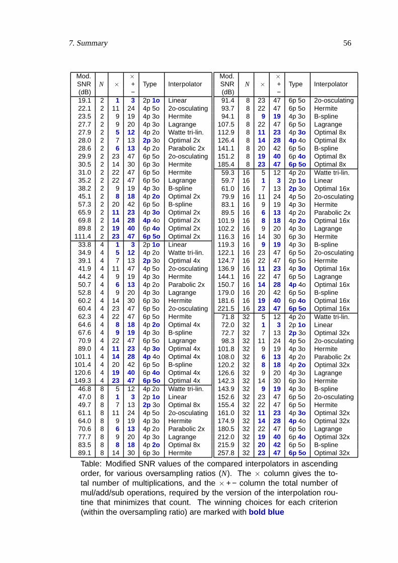
7. Summary 56
Mod. ×SNR N × + Type Interpolator(dB) −19.1 2 1 3 2p 1o Linear22.1 2 11 24 4p 5o 2o-osculating23.5 2 9 19 4p 3o Hermite27.7 2 9 20 4p 3o Lagrange27.9 2 5 12 4p 2o Watte tri-lin.28.0 2 7 13 2p 3o Optimal 2x28.6 2 6 13 4p 2o Parabolic 2x29.9 2 23 47 6p 5o 2o-osculating30.5 2 14 30 6p 3o Hermite31.0 2 22 47 6p 5o Hermite35.2 2 22 47 6p 5o Lagrange38.2 2 9 19 4p 3o B-spline45.1 2 8 18 4p 2o Optimal 2x57.3 2 20 42 6p 5o B-spline65.9 2 11 23 4p 3o Optimal 2x69.8 2 14 28 4p 4o Optimal 2x89.8 2 19 40 6p 4o Optimal 2x
111.4 2 23 47 6p 5o Optimal 2x33.8 4 1 3 2p 1o Linear34.9 4 5 12 4p 2o Watte tri-lin.39.1 4 7 13 2p 3o Optimal 4x41.9 4 11 47 4p 5o 2o-osculating44.2 4 9 19 4p 3o Hermite50.7 4 6 13 4p 2o Parabolic 2x52.8 4 9 20 4p 3o Lagrange60.2 4 14 30 6p 3o Hermite60.4 4 23 47 6p 5o 2o-osculating62.3 4 22 47 6p 5o Hermite64.6 4 8 18 4p 2o Optimal 4x67.6 4 9 19 4p 3o B-spline70.9 4 22 47 6p 5o Lagrange89.0 4 11 23 4p 3o Optimal 4x
101.1 4 14 28 4p 4o Optimal 4x101.4 4 20 42 6p 5o B-spline120.6 4 19 40 6p 4o Optimal 4x149.3 4 23 47 6p 5o Optimal 4x
46.8 8 5 12 4p 2o Watte tri-lin.47.0 8 1 3 2p 1o Linear49.7 8 7 13 2p 3o Optimal 8x61.1 8 11 24 4p 5o 2o-osculating64.0 8 9 19 4p 3o Hermite70.6 8 6 13 4p 2o Parabolic 2x77.7 8 9 20 4p 3o Lagrange83.5 8 8 18 4p 2o Optimal 8x89.1 8 14 30 6p 3o Hermite
Mod. ×SNR N × + Type Interpolator(dB) −91.4 8 23 47 6p 5o 2o-osculating93.7 8 22 47 6p 5o Hermite94.1 8 9 19 4p 3o B-spline
107.5 8 22 47 6p 5o Lagrange112.9 8 11 23 4p 3o Optimal 8x126.4 8 14 28 4p 4o Optimal 8x141.1 8 20 42 6p 5o B-spline151.2 8 19 40 6p 4o Optimal 8x185.4 8 23 47 6p 5o Optimal 8x59.3 16 5 12 4p 2o Watte tri-lin.59.7 16 1 3 2p 1o Linear61.0 16 7 13 2p 3o Optimal 16x79.9 16 11 24 4p 5o 2o-osculating83.1 16 9 19 4p 3o Hermite89.5 16 6 13 4p 2o Parabolic 2x
101.9 16 8 18 4p 2o Optimal 16x102.2 16 9 20 4p 3o Lagrange116.3 16 14 30 6p 3o Hermite119.3 16 9 19 4p 3o B-spline122.1 16 23 47 6p 5o 2o-osculating124.7 16 22 47 6p 5o Hermite136.9 16 11 23 4p 3o Optimal 16x144.1 16 22 47 6p 5o Lagrange150.7 16 14 28 4p 4o Optimal 16x179.0 16 20 42 6p 5o B-spline181.6 16 19 40 6p 4o Optimal 16x221.5 16 23 47 6p 5o Optimal 16x71.8 32 5 12 4p 2o Watte tri-lin.72.0 32 1 3 2p 1o Linear72.7 32 7 13 2p 3o Optimal 32x98.3 32 11 24 4p 5o 2o-osculating
101.8 32 9 19 4p 3o Hermite108.0 32 6 13 4p 2o Parabolic 2x120.2 32 8 18 4p 2o Optimal 32x126.6 32 9 20 4p 3o Lagrange142.3 32 14 30 6p 3o Hermite143.9 32 9 19 4p 3o B-spline152.6 32 23 47 6p 5o 2o-osculating155.4 32 22 47 6p 5o Hermite161.0 32 11 23 4p 3o Optimal 32x174.9 32 14 28 4p 4o Optimal 32x180.5 32 22 47 6p 5o Lagrange212.0 32 19 40 6p 4o Optimal 32x215.9 32 20 42 6p 5o B-spline257.8 32 23 47 6p 5o Optimal 32x
Table: Modified SNR values of the compared interpolators in ascendingorder, for various oversampling ratios (N). The × column gives the to-tal number of multiplications, and the × + − column the total number ofmul/add/sub operations, required by the version of the interpolation rou-tine that minimizes that count. The winning choices for each criterion(within the oversampling ratio) are marked with bold blue
8. Pre-emphasis 57
The optimal interpolators are superior (especially with low N) within interpolatorsof same order and samplepoints – no surprise, they were designed to be. Theyalso often require the least operations for a given SNR.
For example, if one wants at least 100dB modified SNR with the least process-ing (total number of operations), the table suggests the following choices for theinterpolator.
6-point, 5th-order optimal 2x with 2x oversampling (111.4dB);4-point, 4th-order optimal 4x with 4x oversampling (101.1dB);4-point, 3rd-order optimal 8x with 8x oversampling (112.9dB);4-point, 2nd-order optimal 16x with 16x oversampling (101.9dB);Parabolic 2x with 32x oversampling (108.0dB).
For higher oversampling ratios (N), linear interpolation is the best choice becauseof its implementation simplicity. At high N, the oversampled signal is usually notwholly generated, but evaluated only at points needed. In this light, the propertyof linear interpolation of operating only on two points is an important quality.
It is outside the scope of this paper to make guesses of the most profitable over-sampling ratio. Also, it shall only be commented that using polynomial interpola-tors with unoversampled input is a choice that can only be made when the qualityis not that important but speed is essential, the most useful interpolators in thatcase being linear and 4-point Hermite, and Watte tri-linear, which is somewherebetween those two in both quality and computational complexity.
8. Pre-emphasis
Compensation for an interpolator passband attenuation can be done with a pre-emphasis filter. Doing the compensation after the whole resampling processwould generally be harder, because the required filter would need to be differentfor different (possible varying) target samplerates. In addition to being harder,post-emphasis would also be less predictable, so pre-emphasis is presumedthroughout this paper.
Design of the oversampling and pre-emphasis filter(s) has been left for the reader.To make this job easier, minmax-error polynomial approximations of the passbandmagnitude frequency responses of the interpolators are given in the following ta-ble, with a maximum error of ±0.001dB. The x variable is the frequency in radi-ans. x = 0 corresponds to 0Hz and x = π to the passband edge frequency, i.e. theNyquist frequency of the original sampledata before upsampling by N.
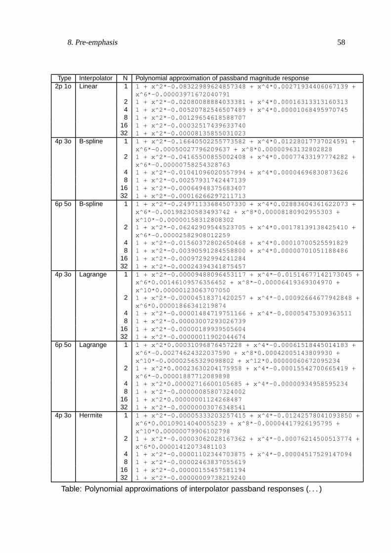
8. Pre-emphasis 58
Type Interpolator N Polynomial approximation of passband magnitude response2p 1o Linear 1 1 + x^2*-0.08322989624857348 + x^4*0.00271934406067139 +
x^6*-0.000039716720407912 1 + x^2*-0.02080088884033381 + x^4*0.000163133131603134 1 + x^2*-0.00520782546507489 + x^4*0.000010684959707458 1 + x^2*-0.00129654618588707
16 1 + x^2*-0.0003251743963374032 1 + x^2*-0.00008135855031023
4p 3o B-spline 1 1 + x^2*-0.16640502255773582 + x^4*0.01228017737024591 +x^6*-0.00050027796209637 + x^8*0.00000963132802828
2 1 + x^2*-0.04165500855002408 + x^4*0.00077433197774282 +x^6*-0.00000758254328763
4 1 + x^2*-0.01041096020557994 + x^4*0.000046968308736268 1 + x^2*-0.00257931742447139
16 1 + x^2*-0.0006494837568340732 1 + x^2*-0.00016266297211713
6p 5o B-spline 1 1 + x^2*-0.24971133684507330 + x^4*0.02883604361622073 +x^6*-0.00198230583493742 + x^8*0.00008180902955303 +x^10*-0.00000158312808302
2 1 + x^2*-0.06242909544523705 + x^4*0.00178139138425410 +x^6*-0.00002582908012259
4 1 + x^2*-0.01560372802650468 + x^4*0.000107005255918298 1 + x^2*-0.00390591284558800 + x^4*0.00000701051188486
16 1 + x^2*-0.0009729299424128432 1 + x^2*-0.00024394341875457
4p 3o Lagrange 1 1 + x^2*-0.00009488096453117 + x^4*-0.01514677142173045 +x^6*0.00146109576356452 + x^8*-0.00006419369304970 +x^10*0.00000123063707050
2 1 + x^2*-0.00004518371420257 + x^4*-0.00092664677942848 +x^6*0.00001866341219874
4 1 + x^2*-0.00001484719751166 + x^4*-0.000054753093635118 1 + x^2*-0.00003007293026739
16 1 + x^2*-0.0000018993950560432 1 + x^2*-0.00000011902044674
6p 5o Lagrange 1 1 + x^2*0.00031096876457228 + x^4*-0.00061518445014183 +x^6*-0.00274624322037590 + x^8*0.00042005143809930 +x^10*-0.00002565329098802 + x^12*0.00000060672095234
2 1 + x^2*0.00023630204175958 + x^4*-0.00015542700665419 +x^6*-0.00001887712089898
4 1 + x^2*0.00002716600105685 + x^4*-0.000009349585952348 1 + x^2*-0.00000085807324002
16 1 + x^2*0.0000000112426848732 1 + x^2*-0.00000003076348541
4p 3o Hermite 1 1 + x^2*-0.00005333203257415 + x^4*-0.01242578041093850 +x^6*0.00109014040055239 + x^8*-0.00004417926195795 +x^10*0.00000079906102798
2 1 + x^2*-0.00003062028167362 + x^4*-0.00076214500513774 +x^6*0.00001412073481103
4 1 + x^2*-0.00001102344703875 + x^4*-0.000045175291470948 1 + x^2*-0.00002463837055619
16 1 + x^2*-0.0000015545758119432 1 + x^2*-0.00000009738219240
Table: Polynomial approximations of interpolator passband responses (. . . )

8. Pre-emphasis 59
Type Interpolator N Polynomial approximation of passband magnitude response6p 3o Hermite 1 1 + x^2*0.00018259576650771 + x^4*-0.00175056161346116 +
x^6*-0.00194042192557450 + x^8*0.00029325481059871 +x^10*-0.00001735249351243 + x^12*0.00000039974321014
2 1 + x^2*0.00016315772984362 + x^4*-0.00019365493638948 +x^6*-0.00001330449384056
4 1 + x^2*0.00001886323801592 + x^4*-0.000011908439529198 1 + x^2*-0.00000337009968184
16 1 + x^2*-0.0000001828073643432 1 + x^2*-0.00000001096502600
6p 5o Hermite 1 1 + x^2*0.00020114336420553 + x^4*-0.00039890572473931 +x^6*-0.00229556927556134 + x^8*0.00033156072749299 +x^10*-0.00001939518424822 + x^12*0.00000044492173307
2 1 + x^2*0.00018449827272179 + x^4*-0.00012076518704688 +x^6*-0.00001656712931157
4 1 + x^2*0.00002231671196743 + x^4*-0.000007653041119078 1 + x^2*-0.00000069755852979
16 1 + x^2*-0.0000000381449621732 1 + x^2*-0.00000005120943160
4p 5o 2o-osculating 1 1 + x^2*-0.00003810731746664 + x^4*-0.01125635108311614 +x^6*0.00093446715934087 + x^8*-0.00003596438901587 +x^10*0.00000062492114797
2 1 + x^2*-0.00002472867620723 + x^4*-0.00069142841070279 +x^6*0.00001220808924164
4 1 + x^2*-0.00000942733874677 + x^4*-0.000041056096268398 1 + x^2*-0.00002230797701725
16 1 + x^2*-0.0000008670878052432 1 + x^2*0.00000015624344717
6p 5o 2o-osculating 1 1 + x^2*0.00016728745643872 + x^4*-0.00033180499542066 +x^6*-0.00214224354648566 + x^8*0.00030186179619621 +x^10*-0.00001731224751541 + x^12*0.00000039135210540
2 1 + x^2*0.00016735375130858 + x^4*-0.00010930555207958 +x^6*-0.00001577254673146
4 1 + x^2*0.00002069410150064 + x^4*-0.000007086014916518 1 + x^2*-0.00000032041779301
16 1 + x^2*0.0000004702248787732 1 + x^2*0.00000011755621969
4p 2o Watte tri-lin. 1 1 + x^2*0.08310376973158973 + x^4*-0.03579156791607385 +x^6*0.00334209365628805 + x^8*-0.00014883957926161 +x^10*0.00000289107920861
2 1 + x^2*0.02073112144393299 + x^4*-0.00219214872746441 +x^6*0.00004267336546731
4 1 + x^2*0.00517460473851293 + x^4*-0.000129805163264268 1 + x^2*0.00130153324464790 + x^4*-0.00000863514074959
16 1 + x^2*0.0003210321142538032 1 + x^2*0.00008109888849582
4p 2o Parabolic 2x 2 1 + x^2*-0.06246359855072939 + x^4*0.00154144387052042 +x^6*-0.00001835446617397
4 1 + x^2*-0.01561067013990179 + x^4*0.000093008796072938 1 + x^2*-0.00385657590779811
16 1 + x^2*-0.0009734470492531632 1 + x^2*-0.00024394574160357
Table: Polynomial approximations of interpolator passband responses (. . . )

9. Conclusion 60
Type Interpolator N Polynomial approximation of passband magnitude response2p 3o Optimal 2x 2 1 + x^2*-0.02554619677843794 + x^4*0.00024013379174846
Optimal 4x 4 1 + x^2*-0.00574208273496733 + x^4*0.00001315216245712Optimal 8x 8 1 + x^2*-0.00135618642176540Optimal 16x 16 1 + x^2*-0.00033233240729770Optimal 32x 32 1 + x^2*-0.00008223446937757
4p 2o Optimal 2x 2 1 + x^2*-0.06789983241024726 + x^4*0.00187396896433240 +x^6*-0.00002473496367671
Optimal 4x 4 1 + x^2*-0.02170313823333328 + x^4*0.00015782661814829Optimal 8x 8 1 + x^2*-0.00728405982348531 + x^4*0.00001497426641413Optimal 16x 16 1 + x^2*-0.00279971126703223Optimal 32x 32 1 + x^2*-0.00119086264779340
4p 3o Optimal 2x 2 1 + x^2*-0.05172434622344999 + x^4*0.00118064718929264 +x^6*-0.00001377425931894
Optimal 4x 4 1 + x^2*-0.01252685934677141 + x^4*0.00006772267827786Optimal 8x 8 1 + x^2*-0.00305463592329826Optimal 16x 16 1 + x^2*-0.00076445772774392Optimal 32x 32 1 + x^2*-0.00019096370951489
4p 4o Optimal 2x 2 1 + x^2*-0.05288134845267101 + x^4*0.00123174456487270 +x^6*-0.00001459486840119
Optimal 4x 4 1 + x^2*-0.01209875686296254 + x^4*0.00006330069200420Optimal 8x 8 1 + x^2*-0.00293014841707120Optimal 16x 16 1 + x^2*-0.00073452725013589Optimal 32x 32 1 + x^2*-0.00018375385546417
6p 4o Optimal 2x 2 1 + x^2*-0.09926567184099210 + x^4*0.00436972559074357 +x^6*-0.00011145259389693 + x^8*0.00000150855440787
Optimal 4x 4 1 + x^2*-0.04104326668505586 + x^4*0.00054795446283906 +x^6*-0.00000365948234725
Optimal 8x 8 1 + x^2*-0.01684372350477612 + x^4*0.00006032275579243Optimal 16x 16 1 + x^2*-0.00764482449535352 + x^4*0.00000744158606948Optimal 32x 32 1 + x^2*-0.00357265950908555
6p 5o Optimal 2x 2 1 + x^2*-0.08084154876655289 + x^4*0.00293944745701822 +x^6*-0.00005171508704785
Optimal 4x 4 1 + x^2*-0.01880393544082998 + x^4*0.00015408893922917Optimal 8x 8 1 + x^2*-0.00465275707182741 + x^4*0.00000997264487197Optimal 16x 16 1 + x^2*-0.00114503636967797Optimal 32x 32 1 + x^2*-0.00026762900966793
Table: Polynomial approximations of interpolator passband responses
9. Conclusion
The presented optimal interpolators make it possible to do transparent-qualityresampling for even the most demanding applications with only 2x or 4x over-sampling before the interpolation. Whether this is better than doing a very high-ratio oversampling and using linear interpolation depends on the platform andthe oversampling implementation. Therefore, which interpolator is the best is notconcluded here. You must first decide what quality you need (for example around90dB modified SNR for a transparency of 16 bits) and then see what alternativesthe table given in the summary has to suggest for the oversampling ratios you canafford.