2010

-15

Swis

s Na

tion

al B

ank

Wor

king

Pap

ers

Monetary Policy Response to Oil Price ShocksJean-Marc Natal

The views expressed in this paper are those of the author(s) and do not necessarily represent those of the Swiss National Bank. Working Papers describe research in progress. Their aim is to elicit comments and to further debate.

Copyright ©The Swiss National Bank (SNB) respects all third-party rights, in particular rights relating to works protectedby copyright (information or data, wordings and depictions, to the extent that these are of an individualcharacter).SNB publications containing a reference to a copyright (© Swiss National Bank/SNB, Zurich/year, or similar) may, under copyright law, only be used (reproduced, used via the internet, etc.) for non-commercial purposes and provided that the source is mentioned. Their use for commercial purposes is only permitted with the prior express consent of the SNB.General information and data published without reference to a copyright may be used without mentioning the source.To the extent that the information and data clearly derive from outside sources, the users of such information and data are obliged to respect any existing copyrights and to obtain the right of use from the relevant outside source themselves.

Limitation of liabilityThe SNB accepts no responsibility for any information it provides. Under no circumstances will it accept any liability for losses or damage which may result from the use of such information. This limitation of liability applies, in particular, to the topicality, accuracy, validity and availability of the information.

ISSN 1660-7716 (printed version)ISSN 1660-7724 (online version)

© 2010 by Swiss National Bank, Börsenstrasse 15, P.O. Box, CH-8022 Zurich

1

Monetary Policy Response to Oil Price Shocks

Jean-Marc Natali

First draft: June 15, 2009

This draft: September 2, 2010

Abstract

How should monetary authorities react to an oil price shock? The New Key-nesian literature has concluded that ensuring perfect price stability is optimal.Yet, the contrast between theory and practice is striking: In ation targetingcentral banks typically favor a longer run approach to price stability.The rst contribution of this paper is to show that because oil cost shares

vary with oil prices, policies that perfectly stabilize prices entail large welfarecosts, which explains the reluctance of policymakers to enforce them. The policytrade-o faced by monetary authorities is meaningful because oil (energy) is aninput to both production and consumption.Welfare-based optimal policies rely on unobservables, which makes them hard

to implement and communicate. The second contribution of this paper is thus toanalytically derive a simple interest rate rule that mimics the optimal plan in alldimensions but that only depends on observables: core in ation and the growthrates of output and oil prices.It turns out that optimal policy is hard on core in ation but cushions the

economy against the real consequences of an oil price shock by reacting stronglyto output growth and negatively to oil price changes. Following a Taylor rule orperfectly stabilizing prices during an oil price shock are very costly alternatives.

Keywords: optimal monetary policy, oil shocks, divine coincidence, simplerulesJEL Class: E32, E52, E58

iSwiss National Bank. SNB, P.O. Box, CH—8022 Zurich, Switzerland. Phone: +41—44—631—3973,Fax: +41—44—631—3901, Email: jean-marc.natal@snb.ch.I would like to thank seminar participants at the FRBSF for helpful comments. I have also bene ted

from useful suggestions by Richard Dennis, Bart Hobijn, Zheng Liu, Carlos Montoro, Carl E.Walshand John C. Williams. The views expressed here are the responsibility of the author and should notbe interpreted as re ecting the views of the Swiss National Bank. Remaining errors and omissions aremine.

2

1 Introduction

In the last ten years a new macroeconomic paradigm has emerged centered around the

New Keynesian (NK henceforth) model, which is at the core of the more involved and

detailed dynamic stochastic general equilibrium (DSGE) models used for policy analysis

at many central banks. Despite its apparent simplicity, the NK model is built on solid

theoretical foundations and has therefore been used to draw normative conclusions on

the appropriate response of monetary policy to economic shocks. One important result

from this literature is that optimal monetary policy should aim at replicating the real

allocation under exible prices and wages, or natural output, which features constant

average markups and no in ation.

In the case of an oil price shock, the canonical NK prescription to policymakers is

thus fairly simple: Central banks must perfectly stabilize in ation1, even if that leads

to large drops in output and employment. Since the latter are considered e cient,

monetary policy should focus on minimizing in ation volatility. There is a divine

coincidence,2 i.e., an absence of trade-o between stabilizing in ation and stabilizing

the welfare relevant output gap.

The contrast between theory and practice is striking, however. When confronted

with rising commodity prices, policymakers in in ation-targeting central banks do in-

deed perceive a trade-o . They typically favor a long run approach to price stability

by avoiding second-round e ects – when wage in ation a ects in ation expectations

and ultimately leads to upward spiralling in ation – but by letting rst-round e ects

on prices play out. So why the di erence? Do policymakers systematically conduct

irrational, suboptimal policies? Or should we reconsider some of the assumptions em-

bedded in the NK model?

Clearly, this paper is not the rst to examine the consequences of di erent monetary

1As noted by Galí (2008 chapter 6), di erent assumptions on nominal rigidities give rise to di erentde nitions of target in ation. Goodfriend and King (2001) and Aoki (2001) argue that monetary policyshould stabilize the stickiest price. By introducing sticky wages alongside sticky prices, Erceg et al.(2000) and Bodenstein, Erceg and Guerrieri (2008) nd that optimal monetary policy should perfectlystabilize a weighted average of core prices and (negative) wage in ation.

2The expression is from Blanchard and Galí (2007).

3

policy reactions to oil price shocks. In a series of empirical papers, Bernanke et al.

(1997, 2004) and Hamilton and Herrera (2004) simulate counterfactual monetary policy

experiments in order to evaluate the marginal impact of monetary policy on output

and in ation in the aftermath of a typical oil price shock. Unfortunately, these types

of exercises su er from a Lucas’ critique problem so that the discussion remains largely

inconclusive. Moreover, the results do not seem to be robust across di erent monetary

policy regimes (see Kilian and Lewis, 2010). To overcome these di culties, Leduc and

Sill (2004) and Carlstrom and Fuerst (2006), for example, conduct the same type of

exercise in microfounded, calibrated general equilibrium models. Although the results

largely depend on the models speci cations, one general insight from this line of work is

that monetary policy potentially plays an important role in explaining the transmission

of an oil shock to the economy. From a normative point of view, their analysis also

suggests that tough medicine - a policy consisting of perfectly stabilizing prices3 - is the

best policy. Note, however, that this conclusion rests on comparing the stabilization

properties of di erent simple monetary policy rules.

More recently, a rapidly growing literature has started to look into the design of

optimal monetary policy responses to oil price shocks in calibrated or estimated NK

models. Not surprisingly, the ndings largely depend on the rigidities and production

structures assumed. Yet, despite the di erences, most studies come to the conclusion

that there is indeed a trade-o between stabilizing in ation and the welfare relevant

output gap.4 One potential reason - as argued by Blanchard and Galí (2007) (hence-

3Dhawan and Jeske (2007) introduce energy use at the household level and obtain that stabilizingcore in ation instead of headline in ation is preferable.

4Drawing on Erceg et al.’s (2000) fundamental insight, a series of papers attribute the policy trade-o to the simultaneous presence of price and wage stickiness. Bodenstein et al. (2008) and Plante(2009) nd that optimal monetary policy should stabilize a weighted average of core and nominalwage in ation. Winkler (2009) considers anticipated and unanticipated (deterministic) oil shocks andalso nds that optimal policy cannot stabilize, at the same time prices, wages and the welfare relevantoutput gap. Nevertheless, following an oil price shock, optimal policy requires a larger output dropthan under a traditional Taylor rule. This result can be contrasted with Kormilitsina (2009), whonds that optimal policy dampens output uctuations compared to a Taylor rule. Her model is richerthan Winkler’s one and estimated on US data. Montoro (2007) derives the Ramsey optimal policy in aclosed economy setting where oil is a non-produced input in the production function. Despite exiblewages, he still nds a monetary policy trade-o that he attributes to the fact that oil shocks a ectoutput and labour di erently, generating a wedge between the e ects on the utility of consumptionand the disutility of labour when oil and labor are gross complement. Drawing on the work of Barsky

4

forth BG07) - relates to the presence of real wage rigidity in an otherwise canonical NK

model which introduces a time-varying wedge between natural and e cient5 output.

In this case, stabilizing prices (targeting natural output) introduces ine cient output

variations and the divine coincidence does not hold anymore.

Here I focus on an alternative explanation that does not hinge on real wage rigidities

but on the characterization of technology and its interaction with the assumption of

monopolistic competition. The rst contribution of this paper is thus to show that

increases in oil prices lead to a quantitatively meaningful monetary policy trade-o

once it is acknowledged (i) that oil cannot easily be substituted by other factors in the

short run, (ii) that there is no scal transfer available to policymakers to o set the

steady-state distortion due to monopolistic competition, and (iii) that oil is an input

both to production and to consumption (via the impact of the price of crude oil on the

prices of gasoline, heating oil and electricity).

In a nutshell, oil price hikes temporarily lead to higher oil cost shares. The larger

the market distortion due to monopolistic competition, the larger is the e ect of a

given increase in oil price on rms’ real marginal cost and the more important is

the drop in output and real wages required to stabilize prices. This explains why

perfectly stabilizing prices in a non-competitive economy introduces ine cient output

variations and an endogenous monetary policy trade-o . By assuming Cobb-Douglas

production (and thus constant cost shares) or an e cient economy in the steady-state,

the canonical NK model dismisses out of hand the mere possibility of a trade-o .6

and Kilian (2004) and Kilian (2008), Nakov and Pescatori (2009) expand the canonical NK model toinclude an optimization-based model of the oil industry featuring both monopolistic and competitiveoil producers. They show that the deviation of the best targeting rule from strict in ation targeting issubstantial due to ine cient endogenous price markup variations in the oil industry. Finally, openingthe NK model, De Fiore et al. (2006) build a large three-country DSGE model - featuring two oil-importing countries and one oil exporting country - that they estimate on US and EU data. In contrastwith the other papers mentioned above, the authors consider a whole array of shocks and search forthe simple welfare maximizing rule. Their main nding in this context is that the optimal rule reactsstrongly to in ation but accomodates output gap uctuations, suggesting again a policy trade-o .

5The undistorted level of output that would prevail in the absence of nominal frictions in a perfectlycompetitive economy.

6Note that a central bank is usely thought to face a policy trade-o between stabilizing the outputgap and stabilizing in ation. In microfounded models, this trade-o is typically modelled as arisingfrom an exogenous markup shock (see for example Galì, 2008). In contrast, this paper provides anendogenous derivation of a cost-push shock.

5

While conditions (i) and (ii) are necessary to introduce a microfounded monetary

policy trade-o , they are not su cient to explain the policymakers’ concern for the real

consequences of oil price shocks. Hence, this paper stresses that perfectly stabilizing

in ation becomes particularly costly when the impact of higher oil prices on households’

consumption is also taken into account. Changes in oil prices act as a distortionary tax

on labor income and amplify the monetary policy trade-o . The lower the elasticity of

substitution between energy and other consumption goods, the larger is the tax e ect

and the more detrimental are the consequences on employment and output of a given

increase in oil prices. Importantly, these ndings do not hinge on particular functional

forms for production or consumption. All that is needed is that oil cost shares be

allowed to vary with the price of oil.

This paper also shows that central banks can improve on both the perfect price

stability solution and the recommendation of a simple Taylor rule. And the welfare

gains are large. One problem with welfare-based optimal policies, however, is that they

rely on unobservables such as the e cient level of output or various shadow prices. This

makes them di cult to communicate and to implement. The second contribution of this

paper is thus to analytically derive a simple interest rate rule that mimics the optimal

plan along all relevant dimensions but that relies only on observables – namely core

in ation and the growth rates of output and oil prices.7 It turns out that optimal

policy is hard on core in ation but cushions the economy against the real consequences

of an oil price shock by reacting strongly to output growth and negatively to oil price

changes. In other words, the optimal response to a persistent increase in oil price

resembles the typical response of in ation targeting central banks: While long-term

price stability is ensured by a credible commitment to stabilize in ation and in ation

expectations, short-term real interest rates drop right after the shock to help dampen

real output uctuations.

The rest of the paper is structured as follows. Section 2 starts by building a two-

sector NK model where oil enters as a gross complement to both production and con-

7See Orphanides and Willliams (2003) for a thorough discussion of implementable monetary policyrules.

6

sumption, thus featuring both core and headline in ation like in Bodenstein et al.

(2008). Section 3 shows that the oil price shock leads to a monetary policy trade-o

that is increasing in the degree of monopolistic competition and is inversely related to

production and consumption elasticities of substitution. In Section 4, a linear-quadratic

solution to the optimal policy problem in a timeless perspective is derived to show that

the optimal weight on in ation in the policymaker’s loss function decreases with the oil

elasticity of substitution. Section 5 derives a simple, implementable interest rate rule

that replicates the optimal plan. Section 6 revisits the 1979 oil shock and computes

the welfare losses associated with standard alternative policy rules in order to give a

sense of the costs incurred when following suboptimal monetary policies. Finally, since

oil price elasticity is very low in the short run but close to one in the long run8, Sec-

tion 7 highlights that this paper’s ndings are robust to a production framework that

features time-varying elasticities of substitution in the spirit of putty-clay9 models of

energy use.

2 The model

Following Bodenstein et al. (2008) (thereafter BEG08), I assume a two-layer NK

closed-economy setting10 composed of a core consumption good, which takes labor and

oil as inputs, and a consumption basket consisting of the core consumption good and

oil. In order to keep the notations as simple as possible, there is only one source of

nominal rigidity in this economy: core goods prices11 are sticky and rms set prices

according to a Calvo scheme.

In contrast to BEG08, however, I relax the assumption of a unitary elasticity of

substitution between oil and other goods and factors. I also explicitly consider a dis-

8See Pindyck and Rotemberg (1983) for an empirical analysis using cross section data.9See Gilchrist and Williams (2005).10This assumption allows one to ignore income distribution and international risk-sharing related

issues.11Introducing nominal wage stickiness like in BEG08 would not change the thrust of the argument.

As shown by Woodford (2003) and Galí (2008), one can usually de ne a composite index of wageand price in ation such that, for most reasonable calibrations, there is virtually no trade-o betweenstabilizing the composite index and the welfare-relevant output gap.

7

torted economy: There is no scal transfer to neutralize the monopolistic competition

distortion. The model being quite standard (see BEG08) I only present the main build-

ing blocks here. A full description is relegated to Appendix I available on the journal’s

website.

2.1 Households

Households maximize utility out of consumption and leisure. Their consumption basket

is de ned as a CES aggregator of the core consumption goods basket and the

household’s demand for oil 12

=

μ(1 )

1

+1¶

1

, (1)

where is the oil quasi-share parameter and is the elasticity of substitution between

oil and non-oil consumption goods.

Allowing for real wage rigidity (which may re ect some unmodeled imperfection in

the labor market as in BG07), the labor supply condition relates the marginal rate of

substitution between consumption and leisure to the geometric mean of real wages in

periods and 1. ³ ´(1 )

=

μ1

1

¶. (2)

In the benchmark calibration, i.e., unless stated otherwise, real wages are perfectly

exible, i.e., = 0.

2.2 Firms

Aggregating over all rms producing core consumption goods, we get the total demand

for intermediate goods ( ) as a function of the demand for core consumption goods

( ) =

μ( )¶

, (3)

12The consumption basket can be regarded as produced by perfectly competitive consumptiondistributors whose production function mirrors the preferences of households over consumption ofoil and non-oil goods.

8

Each intermediate goods rm produces a good ( ) according to a constant returns-

to-scale technology represented by the CES production function

( ) =³(1 ) ( )

1

+ ( )1´

1, (4)

where ( ) and ( ) are the quantities of oil and labor required to produce ( )

given the quasi-share parameters, , and the elasticity of substitution between labor

and oil, .

The real marginal cost in terms of core consumption goods units is given by:

( ) =

Ã(1 )

μ ¶1+

μ ¶1 ! 11

. (5)

2.3 Government

To close the model, I assume that oil is extracted with no cost by the government,

which sells it to the households and the rms and transfers the proceeds in a lump

sum fashion to the households. I abstract from any other role for the government and

assume that it runs a balanced budget in each and every period so that its budget

constraint is simply given by

= ,

for the total amount of oil supplied.

2.4 Calibration

For the sake of comparability, the model calibration closely follows BEG08. The quar-

terly discount factor is set at 0 993, which is consistent with an annualized real

interest rate of 3 percent. The consumption utility function is chosen to be logarithmic

( = 1) and the Frish elasticity of labor supply is set to unity ( = 1).

In the baseline calibration, I set the consumption, , and production, , oil elas-

ticities of substitution to 0 3.13 Following BEG08, is set such that the energy13Our calibration is on the high side of estimates of short-term oil price elasticity of demand reported

by Hamilton (2009) (ranging from 0.05 to 0.34) but corresponds quite closely to the median estimatereported by Kilian and Murphy (2010).

9

component of consumption (gasoline and fuel plus gas and electricity) equals 6 per-

cent, which is in line with US NIPA data, and is chosen such that the energy share

in production is 2 percent. Prices are assumed to have a duration of four quarters, so

that = 0 75. The core goods elasticity of substitution parameters is set to 6, which

implies a 20 percent markup of (core) prices over marginal costs. Finally, the loga-

rithm of the real price of oil in terms of the consumption goods bundle = log( )

is supposed to follow an AR(1) process ( = 0 95).

3 Divine coincidence?

Because of monopolistic competition in intermediate goods markets, the economy’s

steady state is distorted. Production and employment are suboptimally low. Fully

acknowledging this feature of the economy instead of subsidizing it away for convenience

(as is usually done), entails important consequences for optimal policy when oil is

di cult to substitute in the short run.

This section shows that the divine coincidence breaks down when Cobb-Douglas

production, a hallmark of the canonical NK model, is replaced by CES – or any

production function that implies that oil cost shares vary with changes in oil prices.14

Cobb-Douglas production functions greatly simplify the analysis and permit nice closed-

form solutions, but because they assume a unitary elasticity of substitution between

factors they feature constant cost shares over the cycle regardless of the size of the

monopolistic competition distortion. Following an oil price shock, natural (distorted)

output drops just as much as e cient output and perfectly stabilizing prices is then

the optimal policy to follow.

Yet, the case for a unitary elasticity of substitution between oil and other factors

is not particularly compelling, especially at business cycle frequency. If oil is instead

considered a gross complement for other factors (at least in the short run), the response

of output to an oil price shock will depend on the size of the monopolistic competition

distortion. The larger the distortion, the larger is the dynamic impact of a given oil14See Section 7 for an illustration with a production function featuring time-varying price elasticity

of oil demand: very low elasticity in the short run and unitary elasticity in the long run.

10

price shock on the oil cost share – and therefore on output – in the exible prices

and wages equilibrium. Natural (distorted) output will drop more than e cient output.

Strictly stabilizing in ation in the face of an oil price shock is thus no longer the optimal

policy to follow; the divine coincidence breaks down.15

Perfectly stabilizing prices becomes particularly costly when the impact of higher

oil prices on households’ consumption is also taken into account. As stated in the

introduction, increases in oil prices act as a tax on labor income; the lower the elas-

ticity of substitution, the larger is the tax e ect which ampli es the trade-o faced by

monetary authorities.

Although an accurate welfare analysis requires a second order approximation of

the household’s utility function and the model’s supply side (see Section 4 and Ap-

pendix III), some intuition on the mechanisms at stake can be gained by analyzing

the properties of the log-linearized (see Appendix II for details) model economy at the

FPWE.

3.1 Flexible price and wage equilibrium (FPWE)

Solving the system for = 0 and assuming = 1 and = 0 for simplicity, we get16 :

=f (1 )

+

¸(6)

=f (1 + )

+

¸(7)

and

=f (1 f ) + f(1 f ) (1 f )

(8)

where =[1 1(1 )](1 )( +1)

, = (1 f ) (1 f ) ( + 1) and 0 ( 1)

1 re ecting the degree of monopolistic competition in the economy. Note also thatf ³·´1

is the share of oil in the real marginal cost, f 1 is

15In line with the general theory of the second best (see Lipsey and Lancaster, 1956), monetaryauthorities can aim at a higher level of welfare by trading some of the costs of ine cient outputuctuations against the distortion resulting from more in ation.16Note that lowercase letters denote the percent deviation of each variable with respect to its steady

state (e.g., log¡ ¢

).

11

the share of oil in the CPI, (1 )¡ ¢ 1

is the share of the core good in the

consumption goods basket, and marginal cost is :

0 = = (1 f ) ( ) + f ( )

If oil is considered a gross complement to labor in production ( 1), the oil

price elasticity of real marginal costs, f , is increasing in the degree of monopolistic

competition distortion as measured by 1 . The less competitive the economy, the

larger is f and the more sensitive are real marginal costs to increases in oil prices.

As perfect price stability means constant real marginal costs, the more distorted the

economy’s steady-state, the bigger is the real wage drop required to compensate for

higher oil prices. In equilibrium, labor and output must then fall correspondingly.

Increases in oil prices also act as a tax on labor income when 1; the lower the

elasticity of substitution, the larger the tax e ect which compounds with the e ect of

oil price increases on marginal costs.17 More speci cally, as changes in oil prices a ect

headline more than core prices, increases in oil prices have a di erentiated e ect on real

oil prices faced by consumers, , and (higher) real oil prices faced by rms .18

This discrepancy is exacerbated by the fact that changes in oil prices drive a wedge

between the real wage relevant for households (the consumption real wage, ) and the

real wage faced by rms (the production real wage, ). The lower the elasticity

of substitution between energy and other consumption goods, , the larger is the e ect

of a given increase in oil prices on and the larger is the required drop in real wages

(and in labor and output) to stabilize real marginal costs.

Indeed, equations (6), (7) and (8) show that the response of employment, output

and the real wage are increasing in f and f , which are themselves decreasing in

and .19

17Note that the tax e ect tends to zero when the elasticity of substitution as in this case,g 0, and the solution of the model collapses to the one where oil is an input to production only.18Because immediately after an increase in oil prices, the ratio of core to headline prices deteriorates

( 0).19Note that equation (6) shows that when = = 1, which occurs when the production functions

for intermediate and nal goods are Cobb-Douglas, substitution and income e ects compensate oneanother on the labor market and employment remains constant after an oil price shock ( = = 0).

12

3.2 Endogenous cost-push shock

The cyclical wedge between the natural and e cient levels of output after an oil price

shock – the endogenous cost-push shock – can be analyzed by comparing the log-

linearized ex-price output responses in the distorted ( , natural) and undistorted

( , e cient) economies.20

Starting from equation (7), the cyclical distortion can be written as :

= (1 + )³f f ´

(9)

where I assume = 1 in f and , and 1 in f and .

This cyclical distortion can be mapped into a cost-push shock that enters the New

Keynesian Phillips curve (NKPC henceforth) :

= E +1 + + , (10)

where = is the percent deviation of output with respect to the welfare relevant

output and =¡ ¢

is the cost-push shock. Note that = B for B adecreasing function of and , =

¡1¢(1 ) and = (1 ) ( + )

h(1 )

1+ (1 )

i(see Appendix III and IV for detailed derivations).

First, note that the wedge is constant ( = 0) and the divine coincidence holds

when a scal transfer is available to o set the steady state monopolistic distortion. In

this case, f = f and = . There is no cost-push shock and no policy

trade-o . Second, when production functions are Cobb-Douglas ( = = 1), f =f = and f = so that f f = 0; there is again no-trade-o

and = 0. Third, allowing for gross complementarity ( 1) in a world

without scal transfer, will drop more than after an oil shock as f fwhen 1.

Clearly, the lower and and the larger the steady-state distortion (i.e., the lower

), the larger is the cyclical wedge between and ; the larger is the cost-push

20The social planner’s e cient allocation is the same as the one in the decentralized economy whenprices and wages are exible and there is no steady-state monopolistic distortion ( 1 = 1).The natural allocation, on the other hand, corresponds to the ex-price and wage equilibrium in adistorted economy ( 1).

13

shock. Moreover, note that the elasticity of substitution between energy and other

consumption goods, , plays an important role in amplifying the e ect of oil prices on

the gap between and : The lower , the larger is f , the lower is and the larger

is the di erence f f .

Figure 1 shows the instantaneous response of the gap between natural (YN) and

e cient (Y ) output to a (one period) 1-percent increase in the real price of oil as

a function of , the production elasticity of substitution, and for di erent values of

the consumption elasticity of substitution, .21 The gap is exponentially decreasing in

both the elasticities and . Looking at the northeastern extreme of the gure, where

both elasticities are equal to one (the Cobb-Douglas case), we see that the reaction

of natural and e cient outputs are the same22 (the gap is zero), so that stabilizing

in ation or output at its natural level is welfare maximizing. Lowering the production

elasticity only (along the curve CHI=1) gives rise to a monetary policy trade-o . Yet,

the wedge becomes really large when both the consumption and production elasticities

are small (like on the curve labeled CHI=0.3).

Figure 1

Figure 2 performs a similar exercise, but varies the degree of net steady-state

markups ( 1 1) for di erent values of the elasticities and . Again, the wedge

between e cient and natural output swells for large distortions and low elasticities.

Figure 2

4 Optimal monetary policy

What weight should the central bank attribute to in ation over output gap stabiliza-

tion? Rotemberg and Woodford (1997) and Benigno and Woodford (2005) have shown

that the central bank’s loss function - de ned as the weighted sum of in ation and the

21Note that the amplitude of the gap also depends on the Frish-elasticity of labor supply as measuredby 1 . The smaller (the larger the elasticity), the larger are the labor demand and output dropsneeded to stabilize the real marginal cost, and the larger is the cyclical gap between e cient andnatural output.22Solving equations (A3.13) and (A4.3) in Appendices III and IV for = = = = 1, we get

that = = (1 )(1 ) .

14

welfare relevant output gap - could be derived from (a second order approximation of)

the households utility function, thereby setting a natural criterion to answer this ques-

tion (see Appendix III for details). Section 4.1 shows that the parameters governing

the nominal and real rigidities in the model interact with the elasticities of substitution

(that are assumed smaller than one) and have important consequences on the choice of

policy. For reasonable parameter values, however, the weight on in ation stabilization

remains larger than the one on the output gap, a result also obtained by Woodford

(2003) in a more constrained environment.

Given optimal weights in the central bank loss function, what is the optimal policy

response to an oil price shock? Section 4.2 contrasts the dynamic transmission of oil

price shocks under strict in ation targeting and under the optimal precommitment

policy in a timeless perspective.

4.1 Lambda

Given that the central bank’s objective is to minimize the loss function

E 0

X= 0

0©

2 + 2ª

under the economy constraint, the welfare implications of alternative policies crucially

depend on the value of .23 Figure 3 describes the variation of , the relative weight

assigned to output gap stabilization as a function of the elasticity of substitution

and the degree of price stickiness . Stickier prices (larger ) result in larger price

dispersion and therefore larger in ation costs. In this case, monetary authorities will

be less inclined to stabilize output and, for given elasticities of substitution, decreases

when becomes larger.

But also depends crucially on the elasticities of substitution. The lower the

elasticities, the atter is the New Keynesian Phillips curve (NKPC), the larger is the

sacri ce ratio24, and the more concerned will be the central bank with the distortionary

cost of in ation (i.e., the smaller will be ). Assuming perfectly exible real wages

23Appendix III describes how and the loss function are derived from rst principles.24When the NKPC is at, a large change in output is required to a ect in ation.

15

( = 0), our baseline calibration ( = 0 75, = 0 3) leads to = 0 028, which

implies a targeting rule that places a larger weight on in ation stabilization than on

the output gap (in annual in ation terms, the ratio output gap to in ation stabilization

is 0 022 × 4 = 0 66).25 Note that the focus of policy is very sensitive to the degreeof price stickiness. Setting = 0 5 results in = 0 138 and a policy that sets a larger

weight on output gap stabilization ( 0 138× 4 = 1 48).Figure 3

BG07 argue that the optimal policy choice depends crucially on the degree of real

wage stickiness. Figure 4 veri es this claim by letting the degree of real wage stickiness

vary between = 0 and = 0 9. The larger the real wage stickiness, the larger is

the cost-push shock but the larger is the sacri ce ratio as a relatively larger drop in

labor demand and output is necessary to engineer the required drop in real wages that

stabilizes the real marginal cost and in ation. The central bank will tend to be more

concerned with in ation stabilization and will be smaller when is high. Assuming

= 0 9 and our baseline calibration, Figure 4 shows that = 0 002 ( 0 002×4 = 0 18).Figure 4

4.2 Analyzing the trade-o

How di erent is the transmission of an oil price shock under the optimal precommitment

policy in a timeless perspective characterized by the targeting rule (see Woodford, 2003

and Appendix IV) :

= 1 (11)

which holds for all = 0 1 2 3 , from strict in ation targeting which replicates the

FPWE solution? Figure 5 shows that, assuming = = 0 3, the latter implies an

increase in real interest rates (which corresponds to the expected growth of future con-

sumption), while optimal policy recommends a temporary drop for one year following

25The traditional Taylor rule that places equal weights on output stabilization and in ation stabi-lization would imply = 1 16 with quarterly in ation.

16

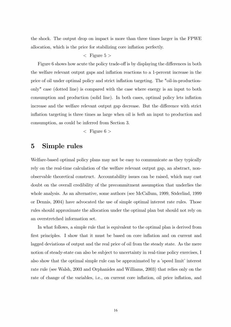
the shock. The output drop on impact is more than three times larger in the FPWE

allocation, which is the price for stabilizing core in ation perfectly.

Figure 5

Figure 6 shows how acute the policy trade-o is by displaying the di erences in both

the welfare relevant output gaps and in ation reactions to a 1-percent increase in the

price of oil under optimal policy and strict in ation targeting. The "oil-in-production-

only" case (dotted line) is compared with the case where energy is an input to both

consumption and production (solid line). In both cases, optimal policy lets in ation

increase and the welfare relevant output gap decrease. But the di erence with strict

in ation targeting is three times as large when oil is both an input to production and

consumption, as could be inferred from Section 3.

Figure 6

5 Simple rules

Welfare-based optimal policy plans may not be easy to communicate as they typically

rely on the real-time calculation of the welfare relevant output gap, an abstract, non-

observable theoretical construct. Accountability issues can be raised, which may cast

doubt on the overall credibility of the precommitment assumption that underlies the

whole analysis. As an alternative, some authors (see McCallum, 1999, Söderlind, 1999

or Dennis, 2004) have advocated the use of simple optimal interest rate rules. Those

rules should approximate the allocation under the optimal plan but should not rely on

an overstretched information set.

In what follows, a simple rule that is equivalent to the optimal plan is derived from

rst principles. I show that it must be based on core in ation and on current and

lagged deviations of output and the real price of oil from the steady state. As the mere

notion of steady-state can also be subject to uncertainty in real-time policy exercises, I

also show that the optimal simple rule can be approximated by a ’speed limit’ interest

rate rule (see Walsh, 2003 and Orphanides and Williams, 2003) that relies only on the

rate of change of the variables, i.e., on current core in ation, oil price in ation, and

17

the growth rate of output; this rule remains close to optimal even when real wages are

sticky.

5.1 The optimal precommitment simple rule

Using the minimal state variable (MSV) approach pioneered by McCallum26, one can

conjecture the no-bubble solution to the dynamic system formed by i) the optimal

targeting rule under the timeless perspective optimal plan and ii) the NKPC equation

to get:

= 11 1 + 12 (12)

= 21 1 + 22 (13)

where for = 1 2 are functions of , , and .

Combining (12) and (13) with the Euler equation for consumption, one can solve

for , the nominal interest rate, and derive the optimal simple rule consistent with the

optimal plan (see Appendix V):

= 111 + 1 + ( + ) 1 (14)

for 221

12 (1 ), 11+ 21, + 21 and ( 1)³1

´.

The optimal interest rate rule is a function of core in ation and current and lagged

output and real oil price, all taken as log deviations from their respective steady states.

Its parameters are functions of households preferences, technology, and nominal fric-

tions.

For a permanent shock, = 1, the rule simpli es to

= 111 +

¡1

1

¢+

¡1

1

¢,

as = 1, and = 0. Looking at and shows that the closer 11 is to 1, the

more precisely a speed limit policy (a rule based on the rate of growth of the variables)

replicates optimal policy as in this case = .

26See McCalllum (1999b) for a recent exposition of the MSV approach.

18

In Section 6, I show that for = 0 95, a degree of persistence which corresponds

closely to the 1979 oil shock, the speed limit policy approximates almost perfectly the

optimal feedback rule despite a value of 11 clearly below 1.

5.2 Optimized simple rules

Analytical solutions to the kind of problem described in Section 5.1 rapidly become

intractable when the number of shocks and lagged state variables is increased (e.g., by

allowing for the possibility of real wage rigidity).

An alternative is to rely on numerical methods in order to estimate a simple rule

mimicking the optimal plan’s allocation along all relevant dimensions. The following

distance minimization algorithm is de ned over the impulse response functions of

variables of interest to the policymakers and searches the parameter space of a simple

interest rate rule that minimizes the distance criterion :

argmin ( ( ) )0 ( ( ) )

where ( ) is an × 1 vector of impulses under the postulated simple interestrate rule, and is its counterpart under the optimal plan.27 The algorithmmatches

the responses of eight variables (output, consumption, hours, headline in ation, core

in ation, real marginal costs, and nominal and real interest rates) over a 20-quarter

period using constrained versions of the following general speci cation of the simple

interest rate rule derived from equation (14) :

= + + 1 1 + + 1 1 + 1 1, (15)

where = ( 1 1 1)0.

I start with a version of the model that assumes perfect real wage exibility and run

the minimum distance algorithm on an unconstrained version of equation (15) and on a

speed limit version where + 1 = 0, + 1 = 0, 1 = 0 and 0. Figure 7

27Another possibility is to search within a predetermined space of simple interest rate rules forthe one that minimizes the central bank loss function (see e.g., Söderlind, 1999 and Dennis, 2004).However as di erent combinations of output gaps and in ation variability could in principle producethe same welfare loss, I rely on IRFs instead.

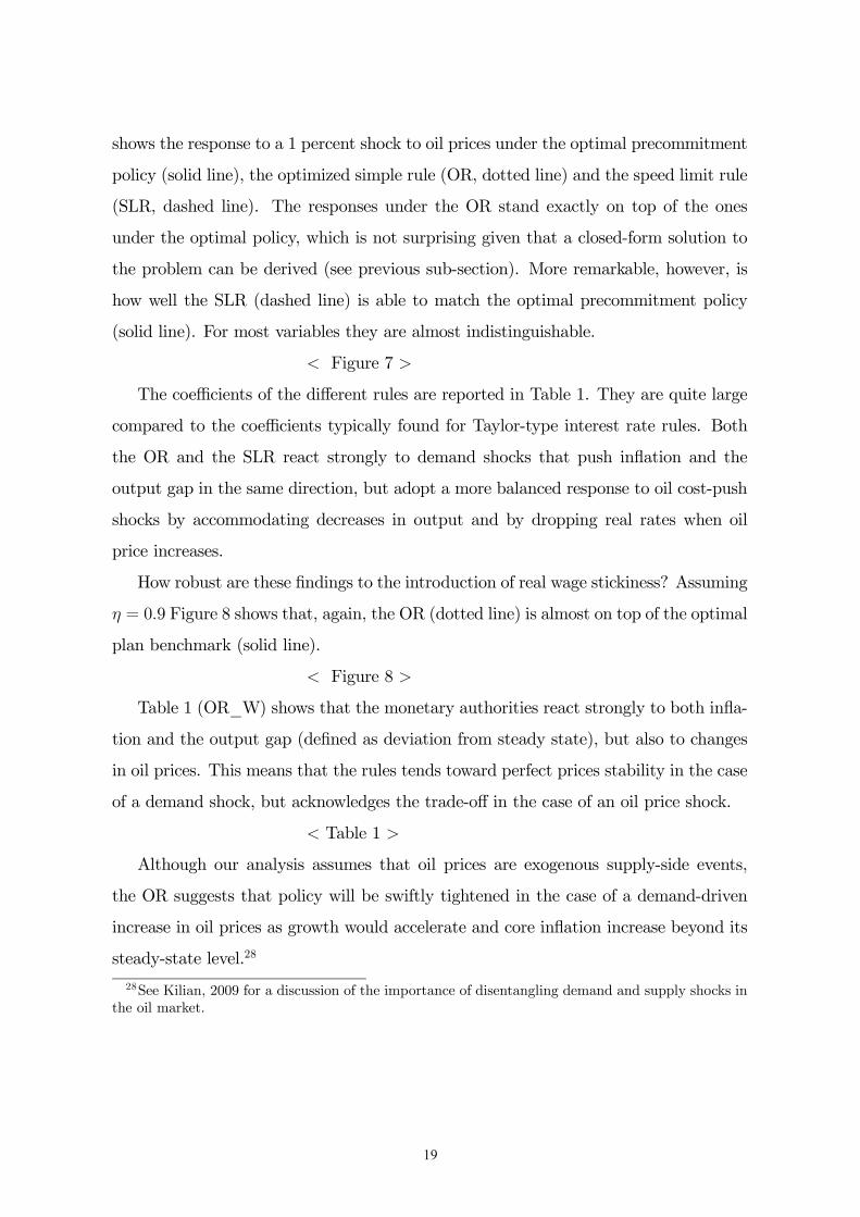
19

shows the response to a 1 percent shock to oil prices under the optimal precommitment

policy (solid line), the optimized simple rule (OR, dotted line) and the speed limit rule

(SLR, dashed line). The responses under the OR stand exactly on top of the ones

under the optimal policy, which is not surprising given that a closed-form solution to

the problem can be derived (see previous sub-section). More remarkable, however, is

how well the SLR (dashed line) is able to match the optimal precommitment policy

(solid line). For most variables they are almost indistinguishable.

Figure 7

The coe cients of the di erent rules are reported in Table 1. They are quite large

compared to the coe cients typically found for Taylor-type interest rate rules. Both

the OR and the SLR react strongly to demand shocks that push in ation and the

output gap in the same direction, but adopt a more balanced response to oil cost-push

shocks by accommodating decreases in output and by dropping real rates when oil

price increases.

How robust are these ndings to the introduction of real wage stickiness? Assuming

= 0 9 Figure 8 shows that, again, the OR (dotted line) is almost on top of the optimal

plan benchmark (solid line).

Figure 8

Table 1 (OR_W) shows that the monetary authorities react strongly to both in a-

tion and the output gap (de ned as deviation from steady state), but also to changes

in oil prices. This means that the rules tends toward perfect prices stability in the case

of a demand shock, but acknowledges the trade-o in the case of an oil price shock.

Table 1

Although our analysis assumes that oil prices are exogenous supply-side events,

the OR suggests that policy will be swiftly tightened in the case of a demand-driven

increase in oil prices as growth would accelerate and core in ation increase beyond its

steady-state level.28

28See Kilian, 2009 for a discussion of the importance of disentangling demand and supply shocks inthe oil market.

20

6 Oil price shocks and US monetary policy

All US recessions since the end of WorldWar II – and the latest vintage is no exception

– have been preceded by a sharp increase in oil prices and an increase in interest

rates.29 But are US recessions really caused by oil shocks, or should the monetary

policy responses to the shocks be blamed for this outcome? Empirical evidence seems

to suggest a role for monetary policy (Bernanke et al. 2004), but its importance remains

di cult to assess. One major stumbling block is the role of expectations. To evaluate

the e ect of di erent monetary policies in the event of an oil price shock one has to take

into account the e ect of those policies on the agents’ expectations, which is typically

not feasible using reduced-form time series models whose estimated parameters are not

invariant to policy (see Lucas, 1976, and Bernanke et al., 2004, for a discussion in the

context of an oil shock).

The alternative approach is to rely on a structural, microfounded model to simulate

counterfactual policy experiments. I start by describing the dynamic behavior of the

economy under di erent monetary policies during the 1979 oil price shock. I have

chosen to focus on this episode for the oil shock was clearly exogenous to economic

activity (Iranian revolution) and as such corresponds to the model de nition of an

oil price shock. I then compute the welfare loss associated with suboptimal policies.

Finally, I compare the optimal rule to standard alternatives in the 2006-2008 oil price

rallye.

6.1 1979 oil price shock

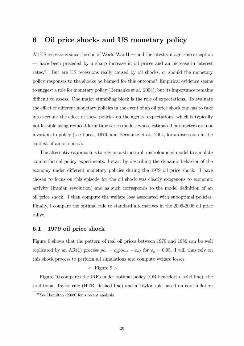
Figure 9 shows that the pattern of real oil prices between 1979 and 1986 can be well

replicated by an AR(1) process = 1 + for = 0 95. I will thus rely on

this shock process to perform all simulations and compute welfare losses.

Figure 9

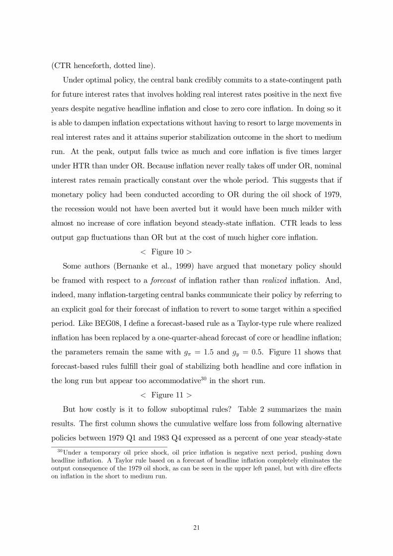
Figure 10 compares the IRFs under optimal policy (OR henceforth, solid line), the

traditional Taylor rule (HTR, dashed line) and a Taylor rule based on core in ation

29See Hamilton (2009) for a recent analysis.

21

(CTR henceforth, dotted line).

Under optimal policy, the central bank credibly commits to a state-contingent path

for future interest rates that involves holding real interest rates positive in the next ve

years despite negative headline in ation and close to zero core in ation. In doing so it

is able to dampen in ation expectations without having to resort to large movements in

real interest rates and it attains superior stabilization outcome in the short to medium

run. At the peak, output falls twice as much and core in ation is ve times larger

under HTR than under OR. Because in ation never really takes o under OR, nominal

interest rates remain practically constant over the whole period. This suggests that if

monetary policy had been conducted according to OR during the oil shock of 1979,

the recession would not have been averted but it would have been much milder with

almost no increase of core in ation beyond steady-state in ation. CTR leads to less

output gap uctuations than OR but at the cost of much higher core in ation.

Figure 10

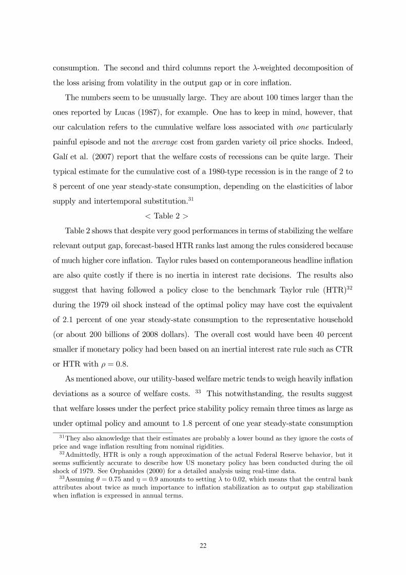
Some authors (Bernanke et al., 1999) have argued that monetary policy should

be framed with respect to a forecast of in ation rather than realized in ation. And,

indeed, many in ation-targeting central banks communicate their policy by referring to

an explicit goal for their forecast of in ation to revert to some target within a speci ed

period. Like BEG08, I de ne a forecast-based rule as a Taylor-type rule where realized

in ation has been replaced by a one-quarter-ahead forecast of core or headline in ation;

the parameters remain the same with = 1 5 and = 0 5. Figure 11 shows that

forecast-based rules ful ll their goal of stabilizing both headline and core in ation in

the long run but appear too accommodative30 in the short run.

Figure 11

But how costly is it to follow suboptimal rules? Table 2 summarizes the main

results. The rst column shows the cumulative welfare loss from following alternative

policies between 1979 Q1 and 1983 Q4 expressed as a percent of one year steady-state

30Under a temporary oil price shock, oil price in ation is negative next period, pushing downheadline in ation. A Taylor rule based on a forecast of headline in ation completely eliminates theoutput consequence of the 1979 oil shock, as can be seen in the upper left panel, but with dire e ectson in ation in the short to medium run.

22

consumption. The second and third columns report the -weighted decomposition of

the loss arising from volatility in the output gap or in core in ation.

The numbers seem to be unusually large. They are about 100 times larger than the

ones reported by Lucas (1987), for example. One has to keep in mind, however, that

our calculation refers to the cumulative welfare loss associated with one particularly

painful episode and not the average cost from garden variety oil price shocks. Indeed,

Galí et al. (2007) report that the welfare costs of recessions can be quite large. Their

typical estimate for the cumulative cost of a 1980-type recession is in the range of 2 to

8 percent of one year steady-state consumption, depending on the elasticities of labor

supply and intertemporal substitution.31

Table 2

Table 2 shows that despite very good performances in terms of stabilizing the welfare

relevant output gap, forecast-based HTR ranks last among the rules considered because

of much higher core in ation. Taylor rules based on contemporaneous headline in ation

are also quite costly if there is no inertia in interest rate decisions. The results also

suggest that having followed a policy close to the benchmark Taylor rule (HTR)32

during the 1979 oil shock instead of the optimal policy may have cost the equivalent

of 2 1 percent of one year steady-state consumption to the representative household

(or about 200 billions of 2008 dollars). The overall cost would have been 40 percent

smaller if monetary policy had been based on an inertial interest rate rule such as CTR

or HTR with = 0 8.

As mentioned above, our utility-based welfare metric tends to weigh heavily in ation

deviations as a source of welfare costs. 33 This notwithstanding, the results suggest

that welfare losses under the perfect price stability policy remain three times as large as

under optimal policy and amount to 1 8 percent of one year steady-state consumption

31They also aknowledge that their estimates are probably a lower bound as they ignore the costs ofprice and wage in ation resulting from nominal rigidities.32Admittedly, HTR is only a rough approximation of the actual Federal Reserve behavior, but it

seems su ciently accurate to describe how US monetary policy has been conducted during the oilshock of 1979. See Orphanides (2000) for a detailed analysis using real-time data.33Assuming = 0 75 and = 0 9 amounts to setting to 0 02, which means that the central bank

attributes about twice as much importance to in ation stabilization as to output gap stabilizationwhen in ation is expressed in annual terms.

23

because of disproportionately large uctuations in the welfare relevant output gap.

6.2 US monetary policy 2006-2008

How does the optimal rule (SLR) compare to actual policy in the US and to usual

benchmarks during the last run up in oil prices, from 2006 to 2008 ? This episode is

of great interest as some recent empirical evidence tends to show that the policy rule

followed by the Federal Reserve was di erent in the post-Volcker period from the one

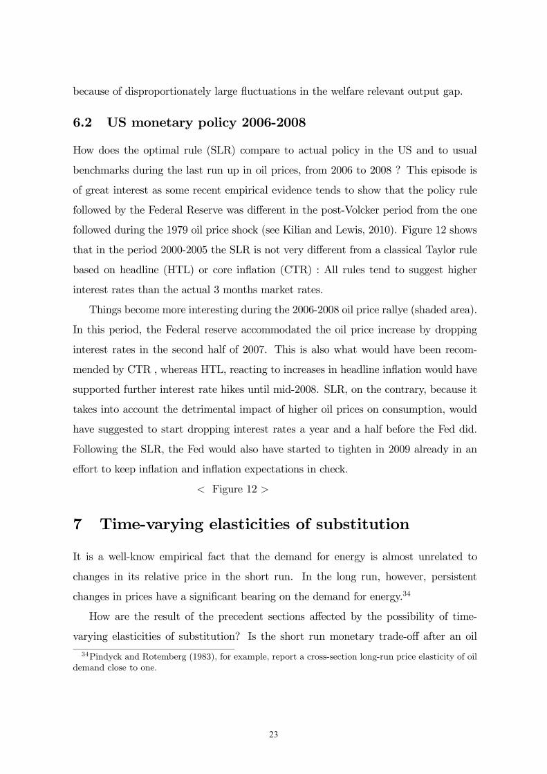
followed during the 1979 oil price shock (see Kilian and Lewis, 2010). Figure 12 shows

that in the period 2000-2005 the SLR is not very di erent from a classical Taylor rule

based on headline (HTL) or core in ation (CTR) : All rules tend to suggest higher

interest rates than the actual 3 months market rates.

Things become more interesting during the 2006-2008 oil price rallye (shaded area).

In this period, the Federal reserve accommodated the oil price increase by dropping

interest rates in the second half of 2007. This is also what would have been recom-

mended by CTR , whereas HTL, reacting to increases in headline in ation would have

supported further interest rate hikes until mid-2008. SLR, on the contrary, because it

takes into account the detrimental impact of higher oil prices on consumption, would

have suggested to start dropping interest rates a year and a half before the Fed did.

Following the SLR, the Fed would also have started to tighten in 2009 already in an

e ort to keep in ation and in ation expectations in check.

Figure 12

7 Time-varying elasticities of substitution

It is a well-know empirical fact that the demand for energy is almost unrelated to

changes in its relative price in the short run. In the long run, however, persistent

changes in prices have a signi cant bearing on the demand for energy.34

How are the result of the precedent sections a ected by the possibility of time-

varying elasticities of substitution? Is the short run monetary trade-o after an oil

34Pindyck and Rotemberg (1983), for example, report a cross-section long-run price elasticity of oildemand close to one.

24

price shock the mere re ection of some CES-related speci city, or is it a more general

argument related to low short-term substitutability in a distorted economy ?

To allow for time-varying elasticities of substitution, I transform the production

processes of Section 2 by introducing a convex adjustment cost of changing the input

mix in production, as in Bodenstein et al. (2007) (see Appendix VI). Figure 13 shows

impulse responses to a 1 percent shock to the price of oil and compares the ex-price

equilibrium allocation with the optimal precommitment policy35 when a scal transfer

is available to neutralize the steady-state ine ciency due to monopolistic competition.

Because of the adjustment costs – which add two state variables to the problem– the

IRFs are not exactly similar to the ones obtained under CES production (see Figure

6). However, the message remains the same: price stability is the optimal policy when

the economy’s steady-state is e cient.

Figure 14 performs the same exercise but allows for the same degree of monopolistic

competition distortion in steady-state as in previous sections (a 20 percent steady-state

markup of core prices over marginal costs). It shows that allowing for time-varying

elasticities of substitution does not a ect the paper’s main nding: In a distorted

equilibrium, an oil price shock introduces a signi cant monetary policy trade-o if the

oil cost share is allowed to vary in the short-run.

Figure 13

Figure 14

8 Conclusion

Most in ation targeting central banks understand their mandate to be ensuring long-

term price stability. Following an oil price shock, however, none of them would be ready

to expose the economy to the type of output and employment drops recommended by

standard New Keynesian theory for the sake of stabilizing prices in the short term.

35Optimal monetary policy is here also derived under the timeless perspective assumption. Sincewe are only interested in the dynamic response of variables to an oil price shock under optimal policy,we do not compute the LQ solution. We directly solve the non-linear model for the Ramsey policythat would maximize utility under the constraint of our model using Andy Levin’s Matlab code (seeLevin 2004, 2005).

25

This paper argues that policies which perfectly stabilize prices entail signi cant welfare

costs, explaining the reluctance of policymakers to enforce them.

Interestingly, I nd that the optimal monetary policy response to a persistent in-

crease in oil price indeed resembles the typical response of in ation targeting central

banks: While long-term price stability is ensured by a credible commitment to keep

in ation and in ation expectations in check, short-term real rates drop right after the

shock to help dampen real output uctuations. By managing expectations e ciently,

central banks can improve on both the exible price equilibrium solution and the rec-

ommendation of simple Taylor rules. Using standard welfare criteria, I reckon that

following a standard Taylor rule in the aftermath of the 1979 oil price shock may have

cost the US household about 2% of annual consumption.

These ndings are based on the assumptions that monetary policy is perfectly

credible and transparent and that agents and the central banks have the right (and

the same) model of the economy. Further work should explore how sensitive the policy

conclusions are to the incorporation of imperfect information and learning into the

analysis. Moreover, further research should establish the robustness of the simple rule

to the incorporation of more shocks into a larger DSGE model. Another potential

limitation of the analysis is that oil price shocks are treated here as exogenous events.

The optimal monetary policy response could vary if the oil price increase was due to

an increase in world aggregate demand instead of an oil supply disruption (see Kilian,

2009, Kilian and Murphy, 2010 and Nakov and Pescatori, 2007 for a rst attempt at

modelling the oil market explicitly). A related issue concerns the treatment of the

open economy aspect. Bodenstein et al. (2007), for example, have shown that the

e ect of an oil price shock on the terms of trade, the trade balance and consumption

depends on the assumption made on the structure of nancial market risk-sharing.

These important considerations are left for future research.

26

References

[1] Atkeson Andrew and Patrick J. Kehoe, 1999. "Models of Energy Use: Putty-Puttyversus Putty-Clay." American Economic Review, Vol. 89, no. 4, 1028-1043.

[2] Barsky, Robert B. and Lutz Kilian. "Oil and TheMacroeconomy Since The 1970s,"Journal of Economic Perspectives, 2004, v18(4,Fall), 115-134.

[3] Benigno, Pierpaolo and Michael Woodford, 2003. "Optimal Monetary and FiscalPolicy: A Linear Quadratic Approach." NBER Working Papers 9905, NationalBureau of Economic Research.

[4] Benigno, Pierpaolo and Michael Woodford, 2005. "In ation Stabilization and Wel-fare: The Case of a Distorted Steady State." Journal of the European EconomicAssociation, MIT Press, vol. 3(6), 1185-1236.

[5] Bernanke, B.S., M. Gertler, and M. Watson, 1997. "Systematic Monetary Policyand the E ects of Oil Price Shocks." Brookings Papers on Economic Activity,91-142.

[6] Bernanke, B.S., M. Gertler, and M.Watson, 2004. "Reply to Oil Shocks and Aggre-gate Macroeconomic Behavior: The Role of Monetary Policy: Comment." Journalof Money, Credit, and Banking 36 (2), 286-291.

[7] Bernanke, Ben S., Laubach, Thomas, Mishkin, Frederic S. and Adam S. Posen,In ation Targeting: Lessons from the International Experience. Princeton, NJ:Princeton Univ. Press, 1999.

[8] Blanchard, Olivier J. and Jordi Gali, 2007. "Real Wage Rigidities and the NewKeynesian Model." Journal of Money, Credit and Banking, Blackwell Publishing,vol. 39(s1), 35-65.

[9] Blanchard, Olivier J. and Jordi Gali, 2007. "The Macroeconomic E ects of OilShocks: Why are the 2000s So Di erent from the 1970s?" NBER Working Papers13368.

[10] Bodenstein, Martin, Erceg, Christopher J. and Luca Guerrieri, 2007. "Oil Shocksand External Adjustment.", FRB International Finance Discussion No. 897.

[11] Bodenstein, Martin, Erceg, Christopher J. and Luca Guerrieri, 2008. "OptimalMonetary Policy with Distinct Core and Headline In ation Rates." FRB Interna-tional Finance Discussion No. 941.

[12] Carlstrom, Charles T. and Timothy S. Fuerst, 2005. "Oil Prices, Monetary Policy,and the Macroeconomy." FRB of Cleveland Policy Discussion Paper No. 10.

[13] Carlstrom, Charles T. and Timothy S. Fuerst, 2006. "Oil Prices, Monetary Pol-icy and Counterfactual Experiments.", Journal of Money, Credit and Banking,Blackwell Publishing, vol. 38, 1945-58.

27

[14] Castillo, Paul, Montoro, Carlos and Vicente Tuesta, 2006. "In ation Premium andOil Price Volatility", CEP Discussion Paper dp0782.

[15] Dennis, Richard, 2004. "Solving for optimal simple rules in rational expectationsmodels." Journal of Economic Dynamics and Control, Volume 28, Issue 8, 1635-1660.

[16] Dhawan, R. and Karsten Jeske, 2007. "Taylor Rules with Headline In ation: ABad Idea", Federal Reserve Bank of Atlanta Working Paper 2007-14.

[17] De Fiore, F., Lombardo, G. and V. Stebunovs, 2006. "Oil Price Shocks, MonetaryPolicy Rules and Welfare", Computing in Economics and Finance, Society forComputational Economics.

[18] Erceg, Christoper J., Dale W. Henderson, and Andrew Levin. 2000. "OptimalMonetary Policy with Staggered Wage and Price Contracts." Journal of MonetaryEconomics, Vol. 46, 281-313.

[19] Galí, Jordi , Gertler, Mark and David Lopez-Salido, 2007. "Markups, Gaps, andthe Welfare Cost of Economic Fluctuations ." Review of Economics and Statistics,vol. 89, 44-59.

[20] Galí, Jordi , Monetary Policy, In ation, and the Business Cycle: An Introductionto the New Keynesian Framework, Princeton, NJ: Princeton Univ. Press, 2008.

[21] Gilchrist, Simon and John C. Williams, 2005. "Investment, Capacity, and Uncer-tainty: a Putty-Clay Approach." Review of Economic Dynamics, Vol. 8, no. 1,1-27.

[22] Goodfriend, Marvin and Robert G. King, 2001."The Case for Price Stability."NBER Working Paper No. W8423.

[23] Hamilton, J.D., and A.M. Herrera, 2004. "Oil Shocks and Aggregate EconomicBehavior: The Role of Monetary Policy: Comment." Journal of Money, Credit,and Banking, 36 (2), 265-286.

[24] Hamilton, J.D., 2009. "Causes and Consequences of the Oil Shock of 2007-08."Brookings Papers on Economic Activity, Conference Volume Spring 2009.

[25] Hughes, J., E., Christopher R. Knittel and Daniel Sperling, 2008, "Evidence of aShift in the Short-Run Price Elasticity of Gasoline Demand." The Energy Journal,Vol. 29, No. 1.

[26] Kilian, L., 2009. "Not all Price Shocks Are Alike: Disentangling Demand andSupply Shocks in the Crude Oil Market", American Economic Review, 99(3),1053-1069.

[27] Kilian, L. and Logan T. Lewis, 2010. "Does the Fed Respond to Oil Price Shocks?",University of Michigan, mimeo.

28

[28] Kilian, Lutz and Dan Murphy, 2010. "The Role of Inventories and SpeculativeTrading in the Global Market for Crude Oil,"CEPR Discussion Papers 7753,C.E.P.R. Discussion Papers.

[29] Kormilitsina, A., 2009. "Oil Price Shocks and the Optimality of Monetary Policy",Southern Methodist University, mimeo.

[30] Krause, Michael U. and Thomas A. Lubik, 2007. "The (ir)relevance of real wagerigidity in the New Keynesian model with search frictions." Journal of MonetaryEconomics, Volume 54, Issue 3, 706-727.

[31] Leduc, Sylvain and Keith Sill, 2004. "A quantitative analysis of oil-price shocks,systematic monetary policy, and economic downturns." Journal of Monetary Eco-nomics, Elsevier, vol. 51(4), 781-808.

[32] Levin, A., Lopez-Salido, J.D., 2004. "Optimal Monetary Policy with EndogenousCapital Accumulation", manuscript, Federal Reserve Board.

[33] Levin, A., Onatski, A., Williams, J., Williams, N., 2005. "Monetary Policy underUncertainty in Microfounded Macroeconometric Models." In: NBER Macroeco-nomics Annual 2005, Gertler, M., Rogo , K., eds. Cambridge, MA: MIT Press.

[34] Lucas, Robert E.,1976. "Econometric Policy Evaluation: A Critique." Carnegie-Rochester Conference Series on Public Policy 1, 19-46.

[35] McCallum, B., 1999. "Issues in the design of monetary policy rules." Taylor, J.,Woodford, M. (Eds.), Handbook of Macroeconomics, North-Holland, New York,pp. 1483—1524.

[36] McCallum, Bennett T., 1999b. "Role of the Minimal State Variable Criterion."NBER Working Paper No. W7087.

[37] McCallum, Bennett T. and Edward Nelson, 2005. "Targeting vs. Instrument Rulesfor Monetary Policy." Federal Reserve Bank of St. Louis Review, 87(5), 597-611.

[38] Montoro, Carlos, 2007. "Oil Shocks and Optimal Monetary Policy", Banco Centralde Reserva del Peru, Working Paper Series, 2007-010.

[39] Nakov, A and Andrea Pescatori, 2007. "In ation-Output Gap Trade-o with aDominant Oil Supplier", Federal Reserve Bank of Cleveland, Working Paper 07-10.

[40] Orphanides, Athanasios, 2000. "Activist stabilization policy and in ation: theTaylor rule in the 1970s." Finance and Economics Discussion Series 2000-13, Boardof Governors of the Federal Reserve System (U.S.).

[41] Orphanides, Athanasios and John C.Williams, 2003, "Robust Monetary PolicyRules with Unknown Natural Rates." FEDS Working Paper No. 2003-11.

29

[42] Pindyck, Robert. S. and Julio J. Rotemberg, 1983. "Dynamic Factor Demandsand the E ects of Energy Price Shocks," American Economic Review, Vol. 73,1066-1079.

[43] Plante, M., 2009. "How Should Monetary Policy Respond to Exogenous Changesin the Relative Price of Oil?", Center for Applied Economics and Policy ResearchWorking Paper #013-2009, Indiana University.

[44] Sims C., and T. Zha., 2006. "Does Monetary Policy Generate Recessions?"Macro-economic Dynamics, 10 (2), 231-272.

[45] Söderlind, P., 1999. "Solution and estimation of RE macromodels with optimalpolicy." European Economic Review 43, pp. 813—823.

[46] Yun, Tack, 1996. "Monetary Policy, Nominal Price Rigidity, and Business Cycles."Journal of Monetary Economics, 37, 345-70.

[47] Walsh Carl , 2003. "Speed Limit Policies: The Output Gap and Optimal MonetaryPolicy," American Economic Review, vol. 93(1), 265-278.

[48] Williams, John C., 2003. "Simple rules for monetary policy." Economic Review,Federal Reserve Bank of San Francisco, 1-12.

[49] Winkler R., 2009. "Ramsey Monetary Policy, Oil Price Shocks and Welfare",Christian-Albrechts-Universty of Kiel, mimeo.

[50] Woodford, Michael. Interest and Prices: Foundations of a Theory of MonetaryPolicy, Princeton University Press, 2003.

[51] Woodford, Michael. "In ation targeting and optimal monetary policy", mimeoprepared for the Annual Economic Policy Conference, Federal Reserve Bank ofSt. Louis, October 16-17, 2003.

30

Appendix I: The model

AI.1 Households

There exists a unit mass continuum of in nitely lived households indexed by [0 1],which maximize the discounted sum of present and expected future utilities de ned asfollows

EX=

(( )1

1

( )1+

1 +

), (A1.1)

where ( ) is the consumption goods bundle, ( ) is the (normalized) quantity ofhours supplied by household of type , the constant discount factor satis es 0 1and is a parameter calibrated to ensure that the typical household works eight hoursa day in steady state.In each period, the representative household faces a standard ow budget con-

straint

( ) + ( ) = 1 1 ( ) + ( ) + e ( ) + ( ) , (A1.2)

where ( ) is a non-state-contingent one period bond, is the nominal gross interestrate, is the CPI, e ( ) is the household share of the rms’ dividends and ( ) isa lump sum scal transfer to the household of the pro ts from sovereign oil extractionactivities.Because the labor market is perfectly competitive, I drop the index such that

( ) =R 10

( ) , and I write the consumption goods bundle36 as a CESaggregator of the core consumption goods basket and the household’s demand foroil

=

μ(1 )

1

+1¶

1

, (A1.3)

where is the oil quasi-share parameter and is the elasticity of substitution betweenoil and non-oil consumption goods.Households determine their consumption, savings, and labor supply decisions by

maximizing (A1.1) subject to (A1.2). This gives rise to the traditional Euler equation

1 = E½μ

+1

¶+1

¾, (A1.4)

which characterizes the optimal intertemporal allocation of consumption and whererepresents headline in ation.Allowing for real wage rigidity (which may re ect some unmodeled imperfection in

the labor market as in BG07), the labor supply condition relates the marginal rate of

36The consumption basket can be regarded as produced by perfectly competitive consumptiondistributors whose production function mirrors the preferences of households over consumption ofoil and non-oil goods.

31

substitution between consumption and leisure to the geometric mean of real wages inperiods and 1. ³ ´(1 )

=

μ1

1

¶. (A1.5)

In the benchmark calibration, i.e., unless stated otherwise, = 0; real wages areperfectly exible and equal to the marginal rate of substitution between labor andconsumption in all periods.Finally, households optimally divide their consumption expenditures between core

and oil consumption according to the following demand equations:

= (1 ) , (A1.6)

= , (A1.7)

where is the relative price of the core consumption good and isthe relative price of oil in terms of the consumption good bundle and where

=¡(1 ) 1 + 1

¢ 11 (A1.8)

represents the overall consumer price index (CPI).

AI.2 Firms

Core goods producers

I assume that the core consumption good is produced by a continuum of perfectlycompetitive producers indexed by [0 1] that use a set of imperfectly substitutableintermediate goods indexed by [0 1]. In other words, core goods are produced viaa Dixit-Stiglitz aggregator

( ) =

μZ 1

0

( )1

¶1

, (A1.9)

where is the elasticity of substitution between intermediate goods. Given the indi-vidual intermediate goods prices, ( ), cost minimization by core goods producersgives rise to the following demand equations for individual intermediate inputs:

( ) =

μ( )¶

( ) , (A1.10)

where =³R 1

0( )1

´ 11

is the core price index.

Aggregating (A1.10) over all core goods rms, the total demand for intermediategoods ( ) is derived as a function of the demand for core consumption goods

( ) =

μ( )¶

, (A1.11)

using the fact that perfect competition in the market for core goods implies ( )

=R 10

( ) .

32

Intermediate goods rms

Each intermediate goods rm produces a good ( ) according to a constant returns-to-scale technology represented by the CES production function

( ) =³(1 ) (H ( ))

1

+ ( ( ))1´

1, (A1.12)

where H is the exogenous Harrod-neutral technological progress whose value is nor-malized to one. ( ) and ( ) are the quantities of oil and labor required to produce( ) given the quasi-share parameters, , and the elasticity of substitution between

labor and oil, .Each rm operates under perfect competition in the factor markets and determines

its production plan so as to minimize its total cost

( ) = ( ) + ( ) , (A1.13)

subject to the production function (A1.12) for given , , and . Their demandsfor inputs are given by

( ) =

μ( )

¶(1 ) ( ) (A1.14)

( ) =

μ( )

¶( ) , (A1.15)

where the real marginal cost in terms of core consumption goods units is given by

( ) =

Ã(1 )

μ ¶1+

μ ¶1 ! 11

. (A1.16)

Price setting

Final goods producers operate under perfect competition and therefore take the pricelevel as given. In contrast, intermediate goods producers operate under monopo-listic competition and face a downward-sloping demand curve for their products, whoseprice elasticity is positively related to the degree of competition in the market. Theyset prices so as to maximize pro ts following a sticky price setting scheme à la Calvo.Each rm contemplates a xed probability of not being able to change its price nextperiod and therefore sets its pro t-maximizing price ( ) to solve

arg max( )

(EX=0

D +e

+ ( )

),

where D + is the stochastic discount factor de ned by D + =³

+

´+and

pro ts are e+ ( ) = ( ) + ( ) + + + ( ) .

33

The solution to this intertemporal maximization problem yields

( )= , (A1.17)

where μ1

¶EX=0

( )¡

+

¢ μ+

+

¶μ+

+

¶+ ,

and

EX=0

( )¡

+

¢1 μ+

+

¶μ+

+

¶Since only a fraction (1 ) of the intermediate goods rms are allowed to reset their

prices every period while the remaining rms update them according to the steady-state in ation rate, it can be shown that the overall core price index dynamics is givenby the following equation

( )1 = ( 1)1 + (1 )

¡( )¢1

(A1.18)

Following Benigno and Woodford (2005), I rewrite equation (A1.18) in terms of thecore in ation rate

( ) 1 = 1 (1 )

μ ¶1, (A1.19)

for

=1

μ ¶+ E {( +1) +1} ,

and

= + E©( +1)

1+1

ª.

AI.3 Government

To close the model, I assume that oil is extracted with no cost by the government,which sells it to the households and the rms and transfers the proceeds in a lumpsum fashion to the households. I abstract from any other role for the government andassume that it runs a balanced budget in each and every period so that its budgetconstraint is simply given by

= ,

for the total amount of oil supplied.

34

A1.4 Market clearing and aggregation

In equilibrium, goods, oil, and labor markets clear. In particular, given the assumptionof a representative household and competitive labor markets, the labor market clearingcondition is Z 1

0

( ) =

Z 1

0

( ) .

Because I assume that the real price of oil is exogenous in the model, thegovernment supplies all demanded quantities at the posted price. The oil marketclearing condition is then given byZ 1

0

( ) +

Z 1

0

( ) = ,

for the total amount of oil supplied.As there is no net aggregate debt in equilibrium,Z 1

0

( ) = = 0,

we can consolidate the government’s and the household’s budget constraints to get theoverall resource constraint

= .

Finally, Calvo price setting implies that in a sticky price equilibrium there is nosimple relationship between aggregate inputs and aggregate output, i.e., there is noaggregate production function. Namely, de ning the e ciency distortion related to

price stickiness for³R 1

0( ( ))

´ 1

, I follow Yun (1996) andwrite the aggregate production relationship

=³(1 )

1

+1´ 1

, (A1.20)

where price dispersion leads to an ine cient allocation of resources given that

:

½1

= 1 ( ) = ( ) all = .

The ine ciency distortion is related to the rate of core in ation by makinguse of the de nition

=

μ ³1

´+ (1 )

¡( )¢ ¶ 1

,

and equations (A1.19) and (A1.17) to get

=

Ã(1 )

μ ¶+

( )

1

! 1

.

35

Appendix II: log-linearized economy

The allocation in the decentralized economy can be summarized by the following veequations. Log-linearizing the labor supply equation (A1.5) (and setting = 0 forexible real wages), the labor demand equation (A1.14), and the real marginal cost(A1.16), gives equations (A2.1), (A2.2), and (A2.3). Substituting out oil consumption(A1.7) in (A1.3) and making use of the overall resource constraint gives (A2.4). Finally,equation (A2.5) is the log-linear version of (A1.8) and describes the evolution of theratio of core to headline price indices as a function of the real price of oil in consumptionunits. Lowercase letters denote the percent deviation of each variable with respect totheir steady states (e.g., log

¡ ¢):

= + (A2.1)

= ( ) + (A2.2)

= (1 f ) ( ) + f ( ) (A2.3)

=f

+ (A2.4)

=f

1 f (A2.5)

where = log( ) is the consumption real wage, = log( ) is the real oil price

in consumption units, = log( ) is the relative price of the core goods in terms of

consumption goods, f ³·´1

is the share of oil in the real marginal cost,

f 1 is the share of oil in the CPI, and (1 )¡ ¢ 1

is the share ofthe core good in the consumption goods basket.Also, the real marginal cost is equal to the inverse of the desired gross markup in the

steady state, itself determined by the degree of monopolistic competition as measuredby the elasticity of substitution between goods . So = 1 in the steady state and

1 when in the perfect competition limit.

Appendix III : Deriving a quadratic loss function

The policy problem originally de ned as maximizing households utility can be rewrittenin terms of a quadratic loss function de ned over the welfare relevant output gapand core in ation as shown in Benigno and Woodford (2005).

36

AIII.1 Second-order approximation of the model supply side

Starting with the labor market, labor demand can be rewritten as:

=

μ ¶(1 ) ,

and the labor supply as:

(1 ) (1 )=

μ1

1

¶Rewriting them in log-deviations from steady state:

= ( ) +

= 1 + (1 ) ( + )

where is the log deviation of the price dispersion measure 1 from its steady stateand measures the distortion due to in ation. Note that these two log-linear equationsare exact transformations of the nonlinear equations.Combining the labor demand and supply with a second-order approximation of the

real marginal cost

= (1 f ) [ ]+f [ ]+1

2f (1 f ) (1 ) [ ]2+

¡k k3¢and a rst-order approximation of the demand for consumption (where the demand forenergy consumption has been substituted out)

=f

+ +¡k k2¢ (A3.1)

we obtain a second-order accurate equilibrium relation linking total hours to outputand the real price of oil

= (1 D ( + )) +D

(1 )M +

W(1 f )

+1

2

D(1 )

W2 (1 )

(1 f )[J + L ]2 +

¡k k3¢+ (A3.2)

whereM [ (1 )

1+B]

1 WB 1 W+W(1+(1 ) )[ (1+(1 )A) (1 )A]

1,

A(1+(1 ) )

³1

´+

(1+(1 ) )

³ ´,

37

W (1 )1+ (1 )

,

1 W (1+(1 ) )1+ (1 )

,J (1 ) ( + ),L (1 )

(1+(1 ) W)B (1 + f (1 ) ) (1 + (1 )A),

D = (1 ) W(1 )

As the price dispersion measure can be written as

=

Ã(1 )

μ ¶+

( )

1

! 1

,

Benigno and Woodford (2004) demonstrate that – the log deviation of the pricedispersion measure – has a second-order approximation that depends only on second-order in ation terms and lagged dispersion

X= 0

0 = ( 0 1) +1

2

X= 0

0

2

2+

¡k k3¢ . (A3.3)

AIII.2 Second-order approximation to NKPC

In this section I derive a second-order approximation to the NKPC, which can be usedto substitute out the term linear in in the second-order approximation to utilitywhen the steady state is distorted.I start by writing a second-order approximation to the model in ation/marginal

cost nexus. For convenience, I rewrite from the main text

=

μ1

¶μ ¶+ ( +1) +1

=

μ ¶+ ( +1)

1+1

=

"1 ( ) 1

1

# 11

Taking a second-order approximation of the three preceding equations, I followBenigno and Woodford (2004) and Castillo et al. (2006) and express the NKPC as

= +1

2[2 ( + ) + ] +

1

22 + +1 +

¡k k3¢ (A3.4)

where I de ne the auxiliary variable

= +1

2

μ1

1+

¶( )2 +

1

2(1 )

38

and the linear expansion of

= 2 ( + ) + +

μ2 1

1+1 + +1

¶.

Using the rst-order37 approximation of and and a second-order approxima-tion of , I write

=W 1 + (1 ) ( + )W+ (1 ) W + B+1

2

(1 )

(1 f )W2 (1 W) [(1 ) ( + ) + L ]2

+¡k k3¢+

which I substitute in (A3.4) to get

= + + W+1

2

¡2 + 2 + 2

¢+1

22 + +1 +

¡k k3¢ (A3.5)

for(1 ) ( + )WBz (1 )2 ( + )2 + 2 (1 ) ( + ) (1 )W + (1 )2 ( + )2W2

(1 ) ( + )W ( + B) z ( + ) (1 )L+ B (1 )zL2 + 2 B + B2

z 11

W2 (1 W)1

Note that the natural level of output can be found from the preceding equation byrewriting it as

= +z }| {

1 + 1 W +1

21¡

2 + 2 + 2¢+1

21 2

+ +1 +¡k k3¢

and ignoring all second-order terms.

37A second-order approximation is not necessary here as these two variables enter multiplicativelywith .

39

Using the law of iterated expectation and (A3.3), equation (A3.5) can be rewrittenas an in nite discounted sum

X= 0

0 =X= 0

01( 0 ( 0 1))

X= 0

0

½1 + 1

21 ( 2 + 2 + 2)

+12

1 (1 + W) 2

¾+

¡k k3¢ . (A3.6)

AIII.3 Second-order approximation to utility

I take a second-order approximation of the representative household utility function in

=X=

{u ( ) ( )} (A3.7)

The second-order approximation of the rst term is given by

u ( ) = u

½+1

2(1 ) 2

¾+

¡k k3¢+ (A3.8)

Substituting (A3.1) and its square into (A3.8), I get

u ( ) = u

½u +

1

2u 2 + u

¾+

¡k k3¢+ (A3.9)

for u 1, u 1 , u (1 ) and stands for terms independent ofpolicy.

The second term in household utility is approximated by

( ) =

½+1

2(1 + ) 2

¾+

¡k k3¢+ (A3.10)

Substituting (A3.2) and its square in (A3.10) and getting rid of variables indepen-dent of policy, I obtain

( ) =

½+ +

1

22 +

¾+

¡k k3¢+ (A3.11)

for

40

1 D ( + ),W

1,

D(1 )

W2 (1 )(1 )

J 2 + (1 + ) (1 D ( + ))2

D(1 )

h(1 + ) (1 D ( + ))M+W2 (1 )

(1 )JL

i.

Now, since the technology is constant returns to scale, the share of labor in totalcost is equivalent to its share in marginal cost and the following equilibrium relationshipat the steady state

u (1 f ) = ,

which can be used to rewrite total utility 0 by substituting (A3.11) and (A3.9) into(A3.7), to get

0 = ( u )X= 0

0

½+1

22 + +

1

22

¾+

¡k k3¢+ ,

(A3.12)where= (1 f ) ,= (1 ) (1 f ) ,

=³ ´

(1 ) (1 f )

= (1 f ) = W= = W.

For the last step, substituting the expression (A3.6) forP

= 0

0 in (A3.12)obtains

0 = uX= 0

01

2

¡1

¢2

+1

2

¡2 1 2

¢+1

2

¡1 (1 + W) ¢

2 +¡k k3¢+ ,

that can be rewritten equivalently as

0 = uX= 0

01

2

¡1

¢[ ]2

+1

2

¡1 (1 + W) ¢

2 +¡k k3¢+

41

which ends up as the central banks’s loss function to minimize

0 = E 0

X= 0

0©

2 + 2ª+

¡k k3¢+for 1

2u ,

1

1 , and where for = 1 and

= 1 (1 + W) . The output gap = is now the percent deviationof output with respect to the welfare relevant output itself de ned as

1

1= . (A3.13)

The values of and are functions of the model parameters and describe theweights assigned by the central bank to stabilize the welfare relevant output gap andcore in ation. In what follows I summarize this information with , whichdetermines how concerned about the output gap a central bank should be after anoil price shock. Typically, decreases with the sacri ce ratio and the degree of pricestickiness.

Appendix IV: Characterizing optimal policy

As shown in Section 3, acknowledging the low level of short-term substitutability be-tween oil and other factors gives rise to a cyclical distortion coming from the interactionbetween the steady-state e ciency distortion and the oil price shock. In terms of themodel equations, this cyclical distortion is translated into a cost-push shock that entersthe New Keynesian Phillips curve (NKPC henceforth). Taking a log-linear approxi-mation of equation (A1.19) around the zero in ation steady-state yields the standardresult that (core) in ation is a function of next period in ation and this period realmarginal cost: the NKPC

= E +1 + , (A4.1)

where is the log-deviation of real marginal cost from its (distorted) steady stateand =

¡1¢(1 ) is the elasticity of in ation to the real marginal cost.

Substituting the labor market clearing level of the real wage into the real marginalcost equation (A1.16), we can rewrite (A4.1) as

= E +1 + , (A4.2)

where the output gap = measures the deviation between current outputand the natural level of output, and where

=B

(A4.3)

for B a decreasing function of and , the oil production and consumption elasticitiesof substitution (see Appendix III).

42

But (A4.2) can be equivalently rewritten as

= E +1 + + , (A4.4)

for =¡ ¢

the cost-push shock that arises as a direct function of the cyclicalwedge between the natural and the welfare maximizing level of output. and =as de ned in Appendix III.Obviously, the divine coincidence obtains when = , which is the case for= = 1, as shown in Section 3.Following Benigno and Woodford’s (2005) linear-quadratic approach, I circumvent

the usual time consistency issues associated with fully optimal monetary policies byassuming that the central bank is able to commit with full credibility to an optimalpolicy plan which speci es a full set of state-contingent sequences { } =0 thatminimize

E 0

X= 0

0©

2 + 2ª

subject to the following sequence of constraints

= E +1 + + (A4.5)

and a constraint on the initial in ation rate

0 = 0 (A4.6)

where 0 is de ned as the in ation rate in time 0 that is consistent with optimalpolicy in a "timeless perspective" or, in other words, the in ation rate that would havebeen chosen a long time ago and which is consistent with the optimal precommitmentplan.Solving this problem under the timeless perspective gives rise to the following set

of rst-order conditions

= 1 (A4.7)

which are supposed to hold for all = 0 1 2 3 and which characterize the centralbank’s optimal policy response.

Appendix V : Deriving an optimal simple rule

Following McCallum (1999b) and McCallum and Nelson (2004), the no bubble MSVsolution to the system formed by equations (A4.4) and (A4.7) can be written as:

= 11 1 + 12 (A5.1)

= 21 1 + 22 , (A5.2)

43

where for = 1 2 are functions of , and .Because the supply of oil is supposed perfectly elastic at a given exogenous real

price, one can write the following de nitions:

=

= +f

1 f ( 1)

that are used to rewrite the consumption Euler equation in deviation from e cientconsumption as follows:

=1μ

E +1f

1 f E ( +1 )

¶+ E +1 (A5.3)

for = E©

+1

ª= (1 ) .

Combining (A5.1), (A5.2), and (A5.3) leads to

21 1 + 22 =1μ

11 12

1( 1) (1 )

¶+ 21 + 22

which can be solved for :

= ( 11 + 21) 21 1 ( 22 12 22 )

+ ( 1)

μ f1 f

¶| {z }

From (A5.1), = 11 1

12, so that the above equation can be rewritten as:

=11

+ ( 11 + 21) ( + 21) 1 + ,

for =¡

221

12 (1 )¢

11.Finally, substituting = in the above, I get:

=11

+ ( 11 + 21) ( + )

( + 21) ( 1 + 1) +

so

= 111 + 1 + ( + ) 1.

44

Appendix VI : Time varying elasticities

To allow for time-varying elasticities of substitution, I transform the production processesof Section 2 by introducing a convex adjustment cost of changing the input mix in pro-duction, as in Bodenstein et al. (2007) and rede ne equations (A1.12) and (A1.3), suchthat

=³(1 )

1

+£ ¤ 1´ 1

(A6.1)

and

=

μ(1 )

1

+£ ¤ 1

¶1

(A6.2)

The variables and represent the costs of changing the oil intensity inthe production of the core good and the consumption basket, and are supposed to takethe following quadratic form

=

"1

2

μ1 1

1

¶2#(A6.3)

=

"1

2

μ1 1

1

¶2#(A6.4)

This speci cation allows for oil demand to respond quickly to changes in output andconsumption, while responding slowly to relative price changes. In the long-run, theelasticity of substitution is determined by the value of and . Although somewhat adhoc, this form of adjustment costs introduces a time-varying elasticity of substitutionfor oil, an important characteristic of putty-clay models such as in Atkeson and Kehoe(1999) or Gilchrist andWilliams (2005).38 The presence of adjustment costs transformsthe static cost-minimization problem of the representative intermediate rms and nalconsumption goods distributors into forward-looking dynamic ones. They can be re-garded as choosing contingency plans for , , , and that minimize theirdiscounted expected cost of producing and subject to the constraints representedby equations (A6.1) to (A6.4).I calibrate and such that the instantaneous price elasticities of demand

for oil correspond to the baseline calibration chosen in the CES setting of the previoussections. The de facto short-term elasticities are then set to 0 3. In the long run, Iassume a unitary elasticity of substitution ( = = 1) such that (A6.1) and (A6.2)are de facto Cobb-Douglas functions when .

38In putty-clay models of energy use, a large variety of types of capital goods are combined withenergy in di erent xed proportions, making the short-term elasticity of substitution low. In the longerrun, the elasticity goes up as rms invest in capital goods with di erent xed energy intensities.

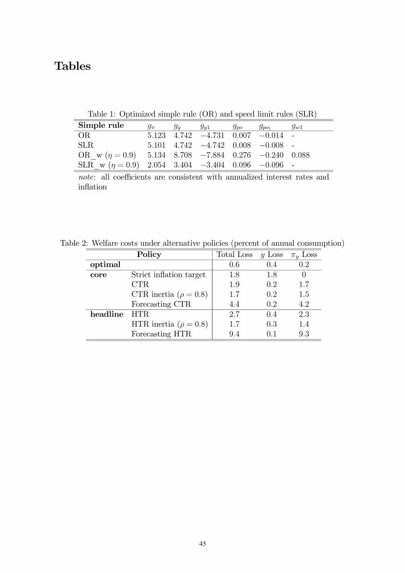
45

Tables

Table 1: Optimized simple rule (OR) and speed limit rules (SLR)Simple rule 1 1 1

OR 5 123 4 742 4 731 0 007 0 014 -SLR 5 101 4 742 4 742 0 008 0 008 -OR_w ( = 0 9) 5 134 8 708 7 884 0 276 0 240 0 088SLR_w ( = 0 9) 2 054 3 404 3 404 0 096 0 096 -

note: all coe cients are consistent with annualized interest rates andin ation

Table 2: Welfare costs under alternative policies (percent of annual consumption)Policy Total Loss Loss Loss

optimal 0 6 0 4 0 2core Strict in ation target 1 8 1 8 0

CTR 1 9 0 2 1 7CTR inertia ( = 0 8) 1 7 0 2 1 5Forecasting CTR 4 4 0 2 4 2

headline HTR 2 7 0 4 2 3HTR inertia ( = 0 8) 1 7 0 3 1 4Forecasting HTR 9 4 0 1 9 3

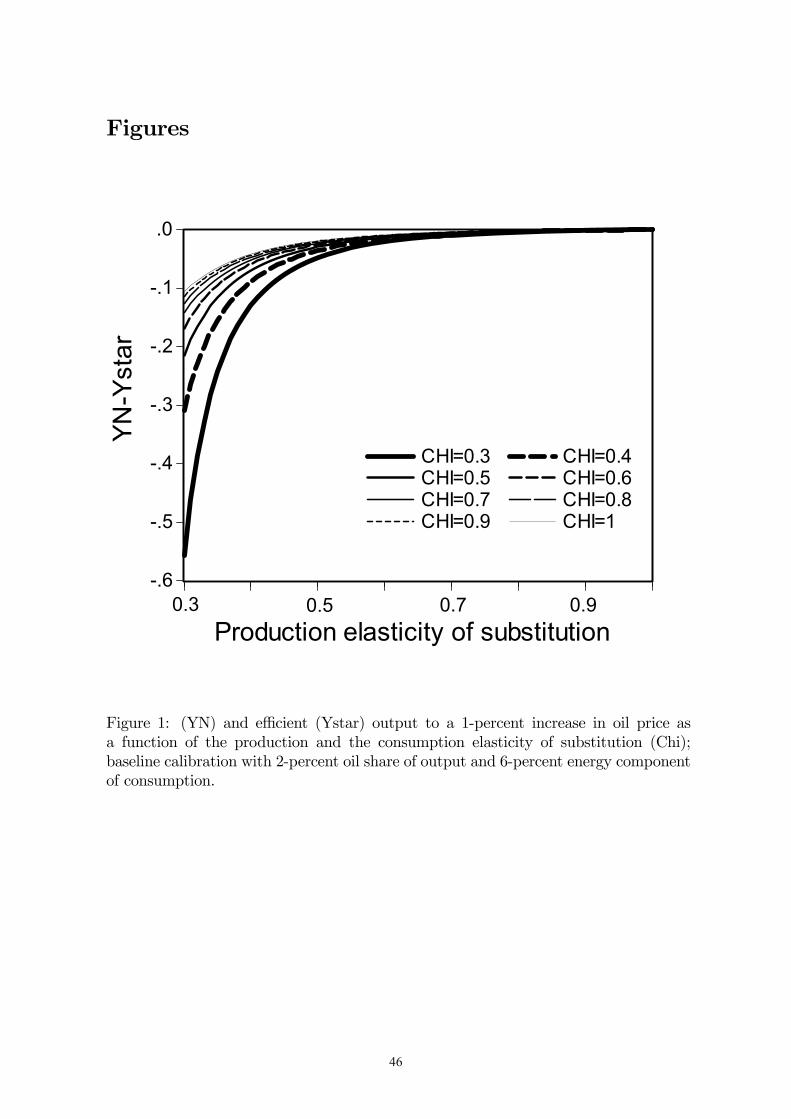
46

Figures

-.6

-.5

-.4

-.3

-.2

-.1

.0

CHI=0.3 CHI=0.4CHI=0.5 CHI=0.6CHI=0.7 CHI=0.8CHI=0.9 CHI=1

0.3 0.5 0.7 0.9Production elasticity of substitution

YN-Y

star

Figure 1: (YN) and e cient (Ystar) output to a 1-percent increase in oil price asa function of the production and the consumption elasticity of substitution (Chi);baseline calibration with 2-percent oil share of output and 6-percent energy componentof consumption.

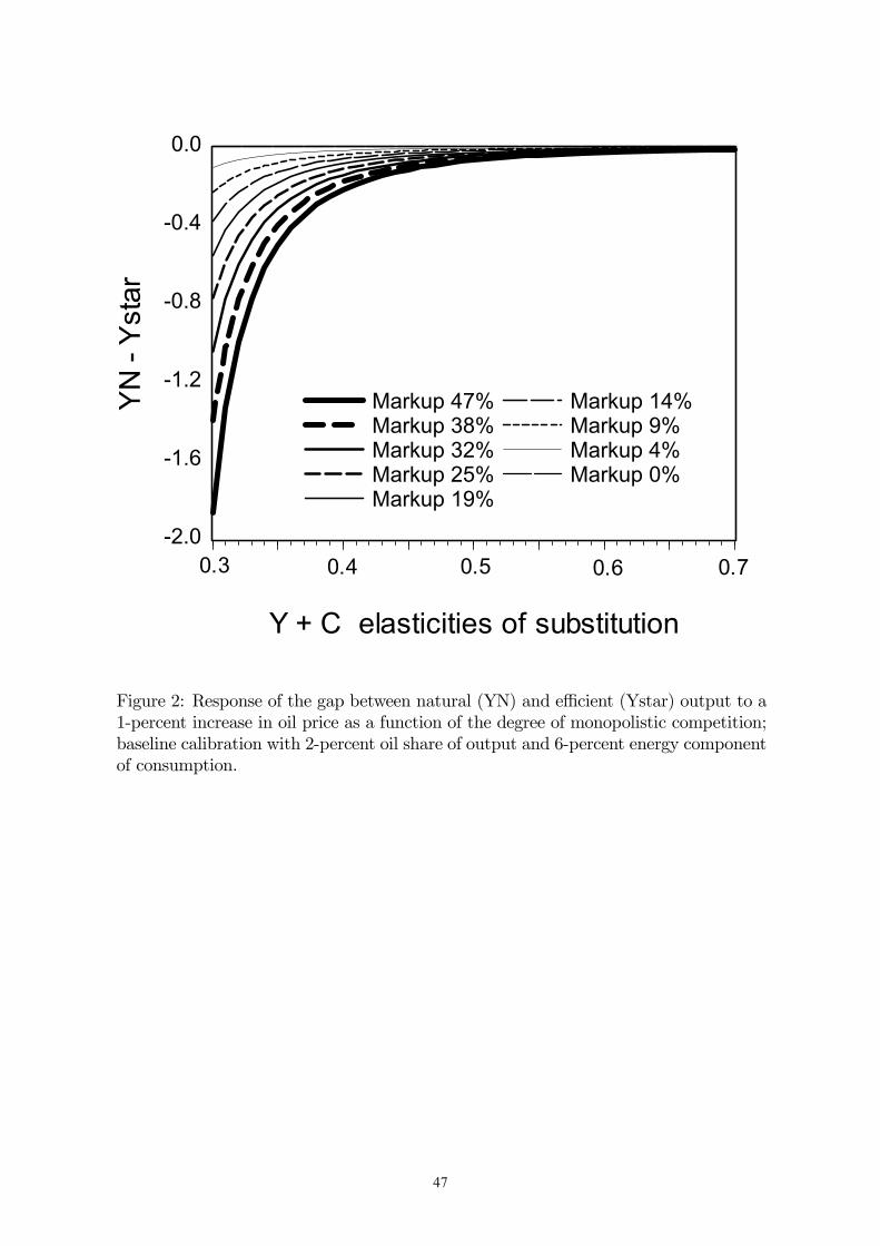
47

-2.0

-1.6

-1.2

-0.8

-0.4

0.0

Markup 47%Markup 38%Markup 32%Markup 25%Markup 19%

Markup 14%Markup 9%Markup 4%Markup 0%

0.3 0.4 0.5 0.6 0.7

Y + C elasticities of substitution

YN

- Y

star

Figure 2: Response of the gap between natural (YN) and e cient (Ystar) output to a1-percent increase in oil price as a function of the degree of monopolistic competition;baseline calibration with 2-percent oil share of output and 6-percent energy componentof consumption.

48

.0

.1

.2

.3

.4

.5

.6teta=0.3teta=0.4teta=0.5teta=0.6

teta=0.7teta=0.8teta=0.9

Lam

bda

Delta

0.1 0.50.3 0.7 0.9

Figure 3: Change in the weight (Lambda) assigned to output gap stabilization as afunction of the elasticities of substitution (Delta) and the degree of price stickiness(teta)

49

.000

.004

.008

.012

.016

.020

.024

.028eta=0eta=0.1eta=0.2eta=0.3

eta=0.4eta=0.5eta=0.6eta=0.7

eta=0.8eta=0.9

Lam

bda

0.1 0.3 0.5 0.7 0.9

Delta

Figure 4: Change in the weight (Lambda) assigned to output gap stabilization as afunction of the elasticities of substitution (Delta) and the degree of real wage rigidity(eta)

50

5 10 15 200.4

0.5

0.6

0.7

0.8

0.9

1OIL PRICE

OptimalFlexible Price

5 10 15 20−0.04

−0.035

−0.03

−0.025

−0.02

OUTPUT

5 10 15 20−0.06

−0.05

−0.04

−0.03

CONSUMPTION

5 10 15 20

−0.03

−0.025

−0.02

−0.015

−0.01

GAP

5 10 15 200

0.01

0.02

0.03

0.04

0.05

0.06

HEADLINE INFLATION

5 10 15 200

0.01

0.02

0.03

0.04

REAL MARGINAL COST

5 10 15 20

0

5

10

x 10−4 CORE INFLATION

5 10 15 20

−8

−6

−4

−2

x 10−3NOM. INTEREST RATE

5 10 15 20−6

−4

−2

0

2

x 10−3REAL INTEREST RATE

Figure 5: Impulse response functions to a 1-percent increase in oil price; compari-son of optimal precommitment monetary policy with exible price equilibrium; CEStechnology with low elasticity ( = = 0 3); baseline calibration.

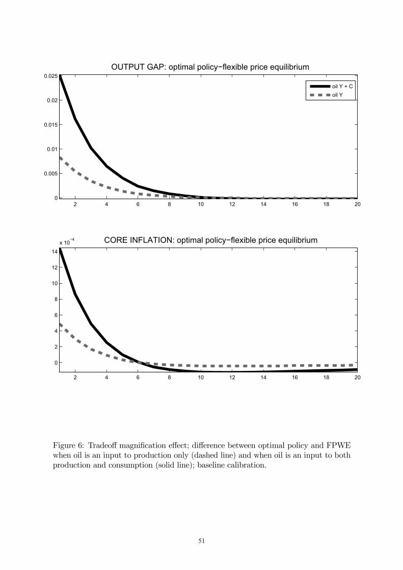
51

2 4 6 8 10 12 14 16 18 200

0.005

0.01

0.015

0.02

0.025OUTPUT GAP: optimal policy−flexible price equilibrium

2 4 6 8 10 12 14 16 18 20

0

2

4

6

8

10

12

14x 10

−4 CORE INFLATION: optimal policy−flexible price equilibrium

oil Y + Coil Y

Figure 6: Tradeo magni cation e ect; di erence between optimal policy and FPWEwhen oil is an input to production only (dashed line) and when oil is an input to bothproduction and consumption (solid line); baseline calibration.

52

5 10 15 200.4

0.5

0.6

0.7

0.8

0.9

1OIL PRICE

OptimalOptimized ruleSpeed rule

5 10 15 20

−0.028

−0.026

−0.024

−0.022

−0.02

−0.018

−0.016

OUTPUT

5 10 15 20−0.045

−0.04

−0.035

−0.03

−0.025

CONSUMPTION

5 10 15 20

−0.02

−0.015

−0.01

GAP

5 10 15 200

0.01

0.02

0.03

0.04

0.05

0.06

HEADLINE INFLATION

5 10 15 200

0.01

0.02

0.03

0.04

0.05REAL MARGINAL COST

5 10 15 20−2

−1

0

1

2

3x 10

−3 CORE INFLATION

5 10 15 20

−8

−6

−4

−2

x 10−3 NOM. INTEREST RATE

5 10 15 20

−6

−5

−4

−3

−2

−1

0

1

x 10−3 REAL INTEREST RATE

Figure 7: Impulse response functions to a 1-percent increase in oil price; comparison ofoptimal precommitment monetary policy with optimized simple rule and speed limitpolicy; CES technology with low elasticity ( = = 0 3); baseline calibration.

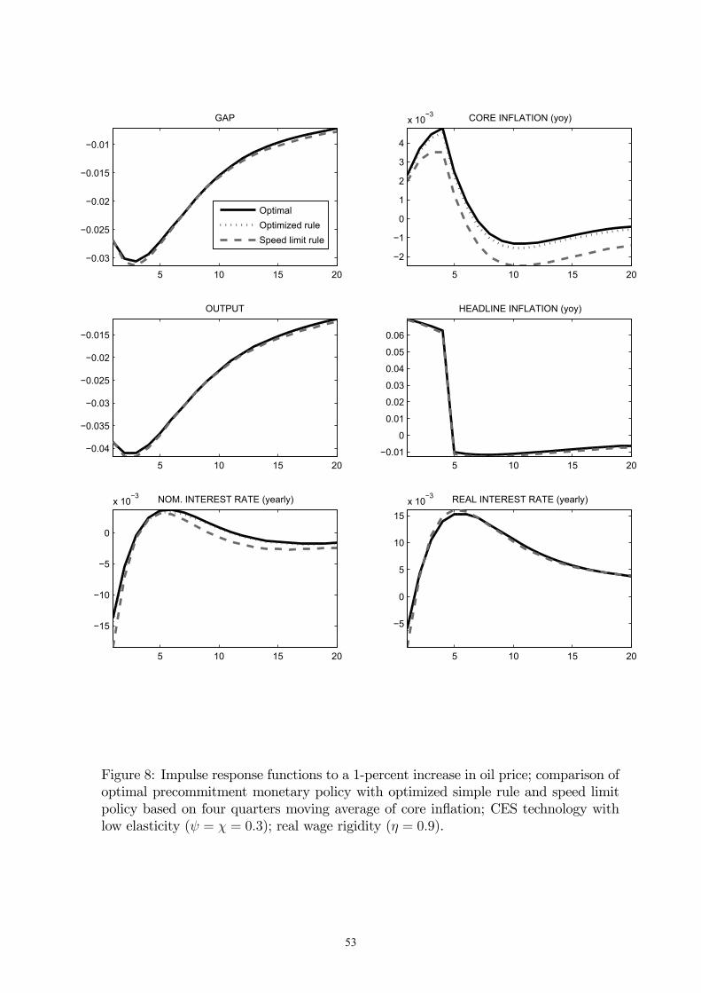
53

5 10 15 20

−0.03

−0.025

−0.02

−0.015

−0.01

GAP

OptimalOptimized ruleSpeed limit rule

5 10 15 20

−2

−1

0

1

2

3

4

x 10−3 CORE INFLATION (yoy)

5 10 15 20

−0.04

−0.035

−0.03

−0.025

−0.02

−0.015

OUTPUT

5 10 15 20−0.01

0

0.01

0.02

0.03

0.04

0.05

0.06

HEADLINE INFLATION (yoy)

5 10 15 20

−15

−10

−5

0

x 10−3 NOM. INTEREST RATE (yearly)

5 10 15 20

−5

0

5

10

15x 10

−3 REAL INTEREST RATE (yearly)

Figure 8: Impulse response functions to a 1-percent increase in oil price; comparison ofoptimal precommitment monetary policy with optimized simple rule and speed limitpolicy based on four quarters moving average of core in ation; CES technology withlow elasticity ( = = 0 3); real wage rigidity ( = 0 9).

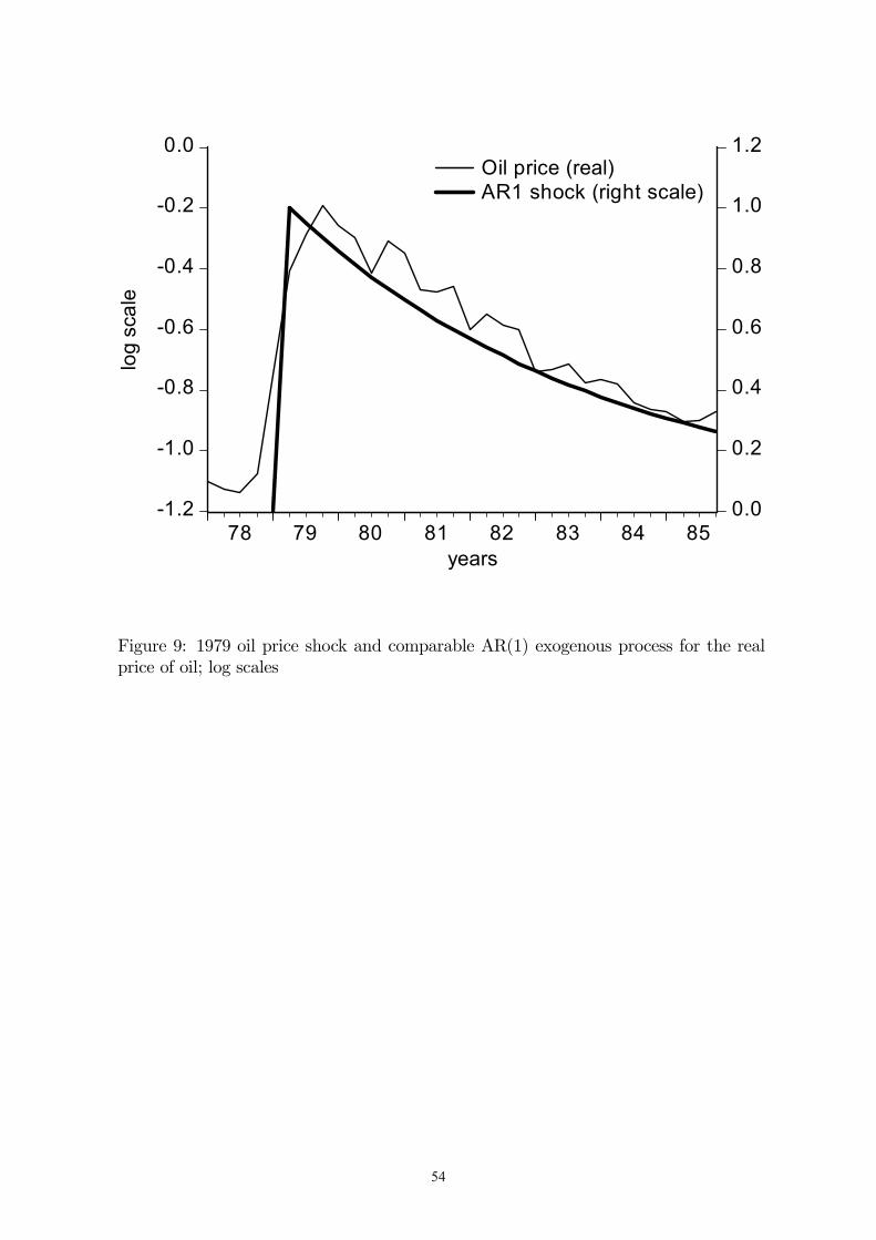
54

-1.2

-1.0

-0.8

-0.6

-0.4

-0.2

0.0

0.0

0.2

0.4

0.6

0.8

1.0

1.2

78 79 80 81 82 83 84 85

Oil price (real)AR1 shock (right scale)

years

log

scal

e

Figure 9: 1979 oil price shock and comparable AR(1) exogenous process for the realprice of oil; log scales

55

5 10 15 20

−0.06

−0.05

−0.04

−0.03

−0.02

−0.01

0GAP

OptimalTaylor coreTaylor headline

5 10 15 200

0.005

0.01

0.015

0.02

0.025

CORE INFLATION (yoy)

5 10 15 20−0.08

−0.07

−0.06

−0.05

−0.04

−0.03

−0.02

−0.01

OUTPUT

5 10 15 20

0

0.02

0.04

0.06

0.08

HEADLINE INFLATION (yoy)

5 10 15 20

0

0.02

0.04

0.06

0.08

0.1

NOM. INTEREST RATE (yearly)

5 10 15 20

0

0.02

0.04

0.06

0.08

REAL INTEREST RATE (yearly)

Figure 10: Impulse response functions to a 1979-like 100% log-increase in oil price;comparison of optimal precommitment monetary policy with simple Taylor rules basedon four quarters moving average values of core or headline in ation; baseline calibration;real wage stickiness ( = 0 9).

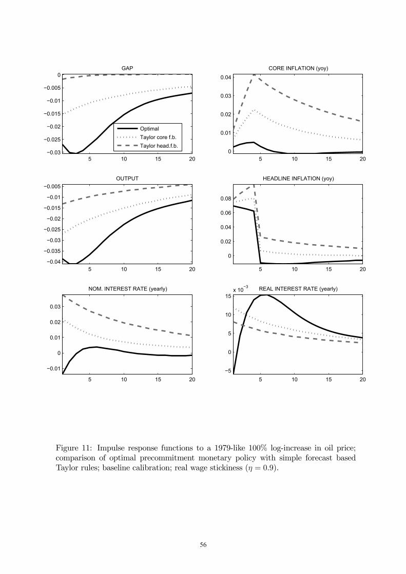
56

5 10 15 20−0.03

−0.025

−0.02

−0.015

−0.01

−0.005

0GAP

OptimalTaylor core f.b.Taylor head.f.b.

5 10 15 200

0.01

0.02

0.03

0.04

CORE INFLATION (yoy)

5 10 15 20−0.04

−0.035

−0.03

−0.025

−0.02

−0.015

−0.01

−0.005OUTPUT

5 10 15 20

0

0.02

0.04

0.06

0.08

HEADLINE INFLATION (yoy)

5 10 15 20

−0.01

0

0.01

0.02

0.03

NOM. INTEREST RATE (yearly)

5 10 15 20−5

0

5

10

15x 10

−3 REAL INTEREST RATE (yearly)

Figure 11: Impulse response functions to a 1979-like 100% log-increase in oil price;comparison of optimal precommitment monetary policy with simple forecast basedTaylor rules; baseline calibration; real wage stickiness ( = 0 9).

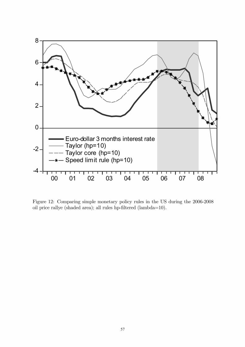
57

-4

-2

0

2

4

6

8

00 01 02 03 04 05 06 07 08

Euro-dollar 3 months interest rateTaylor (hp=10)Taylor core (hp=10)Speed limit rule (hp=10)

Figure 12: Comparing simple monetary policy rules in the US during the 2006-2008oil price rallye (shaded area); all rules hp- ltered (lambda=10).

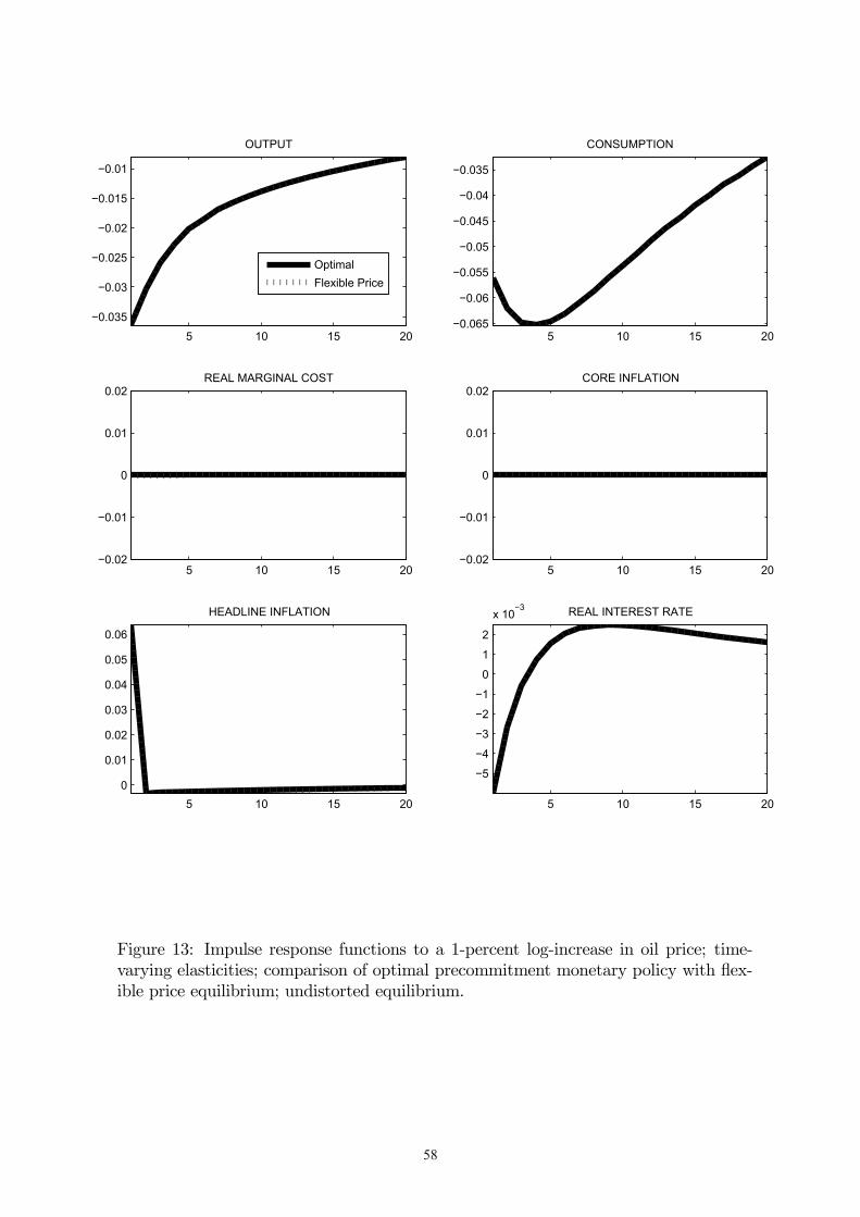
58

5 10 15 20

−0.035

−0.03

−0.025

−0.02

−0.015

−0.01

OUTPUT

OptimalFlexible Price

5 10 15 20−0.065

−0.06

−0.055

−0.05

−0.045

−0.04

−0.035

CONSUMPTION

5 10 15 20−0.02

−0.01

0

0.01

0.02REAL MARGINAL COST

5 10 15 20−0.02

−0.01

0

0.01

0.02CORE INFLATION

5 10 15 200

0.01

0.02

0.03

0.04

0.05

0.06

HEADLINE INFLATION

5 10 15 20

−5

−4

−3

−2

−1

0

1

2

x 10−3 REAL INTEREST RATE

Figure 13: Impulse response functions to a 1-percent log-increase in oil price; time-varying elasticities; comparison of optimal precommitment monetary policy with ex-ible price equilibrium; undistorted equilibrium.

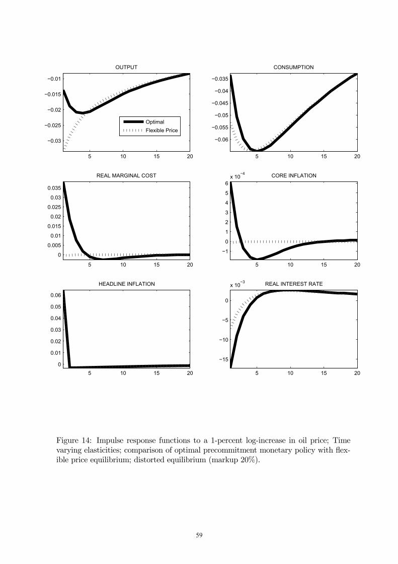
59

5 10 15 20

−0.03

−0.025

−0.02

−0.015

−0.01

OUTPUT

OptimalFlexible Price

5 10 15 20

−0.06

−0.055

−0.05

−0.045

−0.04

−0.035

CONSUMPTION

5 10 15 20

0

0.005

0.01

0.015

0.02

0.025

0.03

0.035

REAL MARGINAL COST

5 10 15 20

−1

0

1

2

3

4

5

6x 10

−4 CORE INFLATION

5 10 15 200

0.01

0.02

0.03

0.04

0.05

0.06

HEADLINE INFLATION

5 10 15 20

−15

−10

−5

0

x 10−3 REAL INTEREST RATE

Figure 14: Impulse response functions to a 1-percent log-increase in oil price; Timevarying elasticities; comparison of optimal precommitment monetary policy with ex-ible price equilibrium; distorted equilibrium (markup 20%).

Swiss National Bank Working Papers published since 2004: 2004-1 Samuel Reynard: Financial Market Participation and the Apparent Instability of

Money Demand 2004-2 Urs W. Birchler and Diana Hancock: What Does the Yield on Subordinated Bank Debt Measure? 2005-1 Hasan Bakhshi, Hashmat Khan and Barbara Rudolf: The Phillips curve under state-dependent pricing 2005-2 Andreas M. Fischer: On the Inadequacy of Newswire Reports for Empirical Research on Foreign Exchange Interventions 2006-1 Andreas M. Fischer: Measuring Income Elasticity for Swiss Money Demand: What do the Cantons say about Financial Innovation? 2006-2 Charlotte Christiansen and Angelo Ranaldo: Realized Bond-Stock Correlation:

Macroeconomic Announcement Effects 2006-3 Martin Brown and Christian Zehnder: Credit Reporting, Relationship Banking, and Loan Repayment 2006-4 Hansjörg Lehmann and Michael Manz: The Exposure of Swiss Banks to

Macroeconomic Shocks – an Empirical Investigation 2006-5 Katrin Assenmacher-Wesche and Stefan Gerlach: Money Growth, Output Gaps and

Inflation at Low and High Frequency: Spectral Estimates for Switzerland 2006-6 Marlene Amstad and Andreas M. Fischer: Time-Varying Pass-Through from Import

Prices to Consumer Prices: Evidence from an Event Study with Real-Time Data 2006-7 Samuel Reynard: Money and the Great Disinflation 2006-8 Urs W. Birchler and Matteo Facchinetti: Can bank supervisors rely on market data?

A critical assessment from a Swiss perspective 2006-9 Petra Gerlach-Kristen: A Two-Pillar Phillips Curve for Switzerland 2006-10 Kevin J. Fox and Mathias Zurlinden: On Understanding Sources of Growth and

Output Gaps for Switzerland 2006-11 Angelo Ranaldo: Intraday Market Dynamics Around Public Information Arrivals 2007-1 Andreas M. Fischer, Gulzina Isakova and Ulan Termechikov: Do FX traders in

Bishkek have similar perceptions to their London colleagues? Survey evidence of market practitioners’ views

2007-2 Ibrahim Chowdhury and Andreas Schabert: Federal Reserve Policy viewed through a Money Supply Lens

2007-3 Angelo Ranaldo: Segmentation and Time-of-Day Patterns in Foreign Exchange

Markets 2007-4 Jürg M. Blum: Why ‘Basel II’ May Need a Leverage Ratio Restriction 2007-5 Samuel Reynard: Maintaining Low Inflation: Money, Interest Rates, and Policy

Stance 2007-6 Rina Rosenblatt-Wisch: Loss Aversion in Aggregate Macroeconomic Time Series 2007-7 Martin Brown, Maria Rueda Maurer, Tamara Pak and Nurlanbek Tynaev: Banking

Sector Reform and Interest Rates in Transition Economies: Bank-Level Evidence from Kyrgyzstan

2007-8 Hans-Jürg Büttler: An Orthogonal Polynomial Approach to Estimate the Term

Structure of Interest Rates 2007-9 Raphael Auer: The Colonial Origins Of Comparative Development: Comment.

A Solution to the Settler Mortality Debate

2007-10 Franziska Bignasca and Enzo Rossi: Applying the Hirose-Kamada filter to Swiss data: Output gap and exchange rate pass-through estimates

2007-11 Angelo Ranaldo and Enzo Rossi: The reaction of asset markets to Swiss National

Bank communication 2007-12 Lukas Burkhard and Andreas M. Fischer: Communicating Policy Options at the Zero

Bound 2007-13 Katrin Assenmacher-Wesche, Stefan Gerlach, and Toshitaka Sekine: Monetary

Factors and Inflation in Japan 2007-14 Jean-Marc Natal and Nicolas Stoffels: Globalization, markups and the natural rate

of interest 2007-15 Martin Brown, Tullio Jappelli and Marco Pagano: Information Sharing and Credit:

Firm-Level Evidence from Transition Countries 2007-16 Andreas M. Fischer, Matthias Lutz and Manuel Wälti: Who Prices Locally? Survey

Evidence of Swiss Exporters 2007-17 Angelo Ranaldo and Paul Söderlind: Safe Haven Currencies

2008-1 Martin Brown and Christian Zehnder: The Emergence of Information Sharing in Credit Markets

2008-2 Yvan Lengwiler and Carlos Lenz: Intelligible Factors for the Yield Curve 2008-3 Katrin Assenmacher-Wesche and M. Hashem Pesaran: Forecasting the Swiss

Economy Using VECX* Models: An Exercise in Forecast Combination Across Models and Observation Windows

2008-4 Maria Clara Rueda Maurer: Foreign bank entry, institutional development and

credit access: firm-level evidence from 22 transition countries 2008-5 Marlene Amstad and Andreas M. Fischer: Are Weekly Inflation Forecasts

Informative? 2008-6 Raphael Auer and Thomas Chaney: Cost Pass Through in a Competitive Model of

Pricing-to-Market 2008-7 Martin Brown, Armin Falk and Ernst Fehr: Competition and Relational Contracts:

The Role of Unemployment as a Disciplinary Device 2008-8 Raphael Auer: The Colonial and Geographic Origins of Comparative Development 2008-9 Andreas M. Fischer and Angelo Ranaldo: Does FOMC News Increase Global FX

Trading? 2008-10 Charlotte Christiansen and Angelo Ranaldo: Extreme Coexceedances in New EU

Member States’ Stock Markets

2008-11 Barbara Rudolf and Mathias Zurlinden: Measuring capital stocks and capital services in Switzerland

2008-12 Philip Sauré: How to Use Industrial Policy to Sustain Trade Agreements 2008-13 Thomas Bolli and Mathias Zurlinden: Measuring growth of labour quality and the

quality-adjusted unemployment rate in Switzerland 2008-14 Samuel Reynard: What Drives the Swiss Franc? 2008-15 Daniel Kaufmann: Price-Setting Behaviour in Switzerland – Evidence from CPI

Micro Data

2008-16 Katrin Assenmacher-Wesche and Stefan Gerlach: Financial Structure and the Impact of Monetary Policy on Asset Prices

2008-17 Ernst Fehr, Martin Brown and Christian Zehnder: On Reputation: A

Microfoundation of Contract Enforcement and Price Rigidity

2008-18 Raphael Auer and Andreas M. Fischer: The Effect of Low-Wage Import Competition on U.S. Inflationary Pressure

2008-19 Christian Beer, Steven Ongena and Marcel Peter: Borrowing in Foreign Currency:

Austrian Households as Carry Traders

2009-1 Thomas Bolli and Mathias Zurlinden: Measurement of labor quality growth caused by unobservable characteristics

2009-2 Martin Brown, Steven Ongena and Pinar Yesin: Foreign Currency Borrowing by

Small Firms 2009-3 Matteo Bonato, Massimiliano Caporin and Angelo Ranaldo: Forecasting realized

(co)variances with a block structure Wishart autoregressive model 2009-4 Paul Söderlind: Inflation Risk Premia and Survey Evidence on Macroeconomic

Uncertainty 2009-5 Christian Hott: Explaining House Price Fluctuations 2009-6 Sarah M. Lein and Eva Köberl: Capacity Utilisation, Constraints and Price

Adjustments under the Microscope 2009-7 Philipp Haene and Andy Sturm: Optimal Central Counterparty Risk Management 2009-8 Christian Hott: Banks and Real Estate Prices 2009-9 Terhi Jokipii and Alistair Milne: Bank Capital Buffer and Risk

Adjustment Decisions

2009-10 Philip Sauré: Bounded Love of Variety and Patterns of Trade 2009-11 Nicole Allenspach: Banking and Transparency: Is More Information

Always Better?

2009-12 Philip Sauré and Hosny Zoabi: Effects of Trade on Female Labor Force Participation 2009-13 Barbara Rudolf and Mathias Zurlinden: Productivity and economic growth in

Switzerland 1991-2005 2009-14 Sébastien Kraenzlin and Martin Schlegel: Bidding Behavior in the SNB's Repo

Auctions 2009-15 Martin Schlegel and Sébastien Kraenzlin: Demand for Reserves and the Central

Bank's Management of Interest Rates 2009-16 Carlos Lenz and Marcel Savioz: Monetary determinants of the Swiss franc

2010-1 Charlotte Christiansen, Angelo Ranaldo and Paul Söderlind: The Time-Varying Systematic Risk of Carry Trade Strategies

2010-2 Daniel Kaufmann: The Timing of Price Changes and the Role of Heterogeneity 2010-3 Loriano Mancini, Angelo Ranaldo and Jan Wrampelmeyer: Liquidity in the Foreign

Exchange Market: Measurement, Commonality, and Risk Premiums 2010-4 Samuel Reynard and Andreas Schabert: Modeling Monetary Policy 2010-5 Pierre Monnin and Terhi Jokipii: The Impact of Banking Sector Stability on the

Real Economy 2010-6 Sébastien Kraenzlin and Thomas Nellen: Daytime is money 2010-7 Philip Sauré: Overreporting Oil Reserves 2010-8 Elizabeth Steiner: Estimating a stock-flow model for the Swiss housing market 2010-9 Martin Brown, Steven Ongena, Alexander Popov, and Pinar Ye,sin: Who Needs

Credit and Who Gets Credit in Eastern Europe? 2010-10 Jean-Pierre Danthine and André Kurmann: The Business Cycle Implications of

Reciprocity in Labor Relations 2010-11 Thomas Nitschka: Momentum in stock market returns: Implications for risk premia

on foreign currencies 2010-12 Petra Gerlach-Kristen and Barbara Rudolf: Macroeconomic and interest rate

volatility under alternative monetary operating procedures 2010-13 Raphael Auer: Consumer Heterogeneity and the Impact of Trade Liberalization:

How Representative is the Representative Agent Framework? 2010-14 Tommaso Mancini Griffoli and Angelo Ranaldo: Limits to arbitrage during the

crisis: funding liquidity constraints and covered interest parity 2010-15 Jean-Marc Natal: Monetary Policy Response to Oil Price Shocks

Swiss National Bank Working Papers are also available at www.snb.ch, section Publications/ResearchSubscriptions or individual issues can be ordered at Swiss National Bank, Fraumünsterstrasse 8, CH-8022 Zurich, fax +41 44 631 81 14, E-mail library@snb.ch