2010

-1Sw

iss

Nati

onal

Ban

k W

orki

ng P

aper

sThe Time-Varying Systematic Risk of Carry Trade StrategiesCharlotte Christiansen, Angelo Ranaldo and Paul Söderlind

The views expressed in this paper are those of the author(s) and do not necessarily represent those of the Swiss National Bank. Working Papers describe research in progress. Their aim is to elicit comments and to further debate.

Copyright ©The Swiss National Bank (SNB) respects all third-party rights, in particular rights relating to works protectedby copyright (information or data, wordings and depictions, to the extent that these are of an individualcharacter).SNB publications containing a reference to a copyright (© Swiss National Bank/SNB, Zurich/year, or similar) may, under copyright law, only be used (reproduced, used via the internet, etc.) for non-commercial purposes and provided that the source is mentioned. Their use for commercial purposes is only permitted with the prior express consent of the SNB.General information and data published without reference to a copyright may be used without mentioning the source.To the extent that the information and data clearly derive from outside sources, the users of such information and data are obliged to respect any existing copyrights and to obtain the right of use from the relevant outside source themselves.

Limitation of liabilityThe SNB accepts no responsibility for any information it provides. Under no circumstances will it accept any liability for losses or damage which may result from the use of such information. This limitation of liability applies, in particular, to the topicality, accuracy, validity and availability of the information.

ISSN 1660-7716 (printed version)ISSN 1660-7724 (online version)

© 2010 by Swiss National Bank, Börsenstrasse 15, P.O. Box, CH-8022 Zurich

1

The Time-Varying Systematic Risk of

Carry Trade Strategies∗

Charlotte Christiansen†

CREATES, Aarhus UniversityAngelo Ranaldo‡

Swiss National Bank

Paul Soderllind§

University of St. Gallen

November 25, 2009

∗The views expressed herein are those of the authors and not necessarily those of the SwissNational Bank (SNB). SNB does not accept any responsibility for the contents and opinionsexpressed in this paper. The authors thank Antonio Mele, as well as seminar participants atthe Arny Ryde Workshop in Financial Economics at Lund University, Swiss National Bank,and CREATES for comments and suggestions. The authors are grateful to an anonymousSNB referee for constructive comments. Christiansen acknowledges support from CREATESfunded by the Danish National Research Foundation and from the Danish Social ScienceResearch Foundation.

†CREATES, School of Economics and Management, Aarhus University, Bartholins Alle10, 8000 Aarhus C, Denmark. Email: CChristiansen@creates.au.dk.

‡Research Department, Swiss National Bank, Switzerland. Email:Angelo.Ranaldo@snb.ch.

§Swiss Institute for Banking and Finance, University of St. Gallen, Rosenbergstr. 52,CH-9000 St. Gallen, Switzerland. Email: Paul.Soderlind@unisg.ch.

2

The Time-Varying Systematic Risk ofCarry Trade Strategies

Abstract: We explain the currency carry trade performance using an asset pric-

ing model in which factor loadings are regime-dependent rather than constant.

Empirical results show that a typical carry trade strategy has much higher expo-

sure to the stock market and is mean-reverting in regimes of high FX volatility.

The findings are robust to various extensions, including more currencies, longer

samples, transaction costs, international stock indices, and other proxies for

volatility and liquidity. Our regime-dependent pricing model provides signifi-

cantly smaller pricing errors than a traditional model. Thus, the carry trade

performance is better explained by its time-varying systematic risk that mag-

nifies in volatile markets—suggesting a partial explanation for the Uncovered

Interest Rate Parity puzzle.

Keywords: carry trade, factor model, FX volatility, liquidity, smooth transi-

tion regression, time-varying betas

JEL Classifications: F31, G15, G11

3

1 Introduction

”(Carry trade) is like picking up nickels in front of steamrollers: you have a

long run of small gains but eventually get squashed.” (The Economist, “Carry

on speculating”, February 22, 2007).

The common definition of currency carry trade is borrowing a low-yielding

asset (for instance, denominated in Japanese yen or Swiss franc) and buying a

higher-yielding asset denominated in another currency. Although this strategy

has proliferated in practice, it is at odds with economic theory. In particular,

the Uncovered Interest Parity (UIP) states that there should be an equality

of expected returns on otherwise comparable financial assets denominated in

two different currencies. Thus, according to the UIP we expect an appreciation

of the low rewarding currency by the same amount as the return differential.

However, there is overwhelming empirical evidence against the UIP theory, see

e.g. Burnside, Eichenbaum and Rebelo (2007) for a recent study.1

One of the most plausible explanations for the UIP puzzle and the long-

lasting carry trade performance is a time-varying risk premium (Fama (1984)).

Relying on this rationale, we analyze whether the systematic risk of a typical

carry trade strategy is time-varying and if it varies across regimes. The literature

proposes several explanations for the carry trade performance such as the expo-

sure to illiquidity spirals (Plantin and Shin (2008)), crash risk (Brunnermeier,

Nagel and Pedersen (2009)) and Peso problems (Farhi and Gabaix (2008))—

although the latter argument is not supported by the substantial payoff remain-

ing in hedged carry trade strategies (see Burnside, Eichenbaum, Kleshchelski

and Rebelo (2008)). By applying an asset pricing approach with factor mimick-

ing portfolios, some recent studies relate excess return of foreign exchanges to

risk factors (e.g. Lustig, Roussanov and Verdelhan (2008)). Here, we propose

to account for FX time-varying risk premia by adopting a related, but differ-

ent, approach. We apply a multi-factor model with explicit factors, but where

the risk exposures are allowed to change according one or more state variables.

This methodology provides a general framework to explain regime-dependent

and non-linear risk-return payoffs. The investigation of regime-switching mod-

els for exchange rates is not new, see Bekaert and Gray (1998), Sarno, Valente

and Leon (2006) and Ichiue and Koyama (2008). Our contribution is to show

that the risk exposure to the stock and bond market in the carry trade is regime

dependent and that regimes are characterized by the level of foreign exchange

1Burnside et al. (2007) also find that forward premium strategies yield very high Sharperatios, but they argue that the carry trade performance is not correlated with traditional riskfactors.

4

volatility. While there have been other papers that point to the importance of

volatility (e.g. Lustig et al. (2008), Menkhoff, Sarno, Schmeling and Schrimpf

(2009)), the present paper is the first to demonstrate that volatility affects the

exposure to stock market risk.

We use a logistic smooth transition regression methodology to explain the

systematic risk of carry trade strategies. In doing so, the state variables have

straightforward economic interpretations such as market risk and illiquidity.

More specifically, we model the regimes by adopting proxies commonly used to

measure market risk (foreign exchange volatility and the V IX) and either mar-

ket or funding illiquidity (the bid-ask spread and the TED). The explanatory

financial factors include equity and bond returns. The asset pricing analysis

shows that the regime-dependent pricing model provides significantly smaller

pricing errors.

Our results on the relevance of the regime dependency of the carry trade risk

shed light on the gamble of currency speculation. By distinguishing between

low and high risk environments, the danger related to carry trade becomes fully

visible. In turbulent times, carry trade significantly increases its systematic

risk and the exposure to other risky allocations. This finding warns against the

apparent attractiveness of carry trade depicted by simple performance measures

such as the Sharpe ratio. Overall, our contribution can be seen as a partial

reconciliation of the UIP puzzle.

This paper is topical due to the ongoing financial crisis which provides a live

experiment for many of the ideas that we explore here.

The structure of the remaining part of the paper is as follows: Section 2

outlines the theoretical motivation and our econometric approach, while Sec-

tion 3 describes the data. Section 4 contains the empirical results; firstly, we

show some preliminary results, secondly, we show the empirical results from

estimating the smooth transition regression model, and thirdly we discuss the

robustness of the results. Finally, we conclude in Section 5.

2 Theoretical and Empirical Framework

2.1 Theoretical Background

This paper combines three strands of literature to model carry trade returns.

First, traditional factor models for exchange rates (McCurdy and Morgan (1991),

Dahlquist and Bansal (2000) and Mark (1988)) suggest that currencies are ex-

posed to equity and bond markets. Second, non-linear patterns in exchange

rate returns emerge from unwinding carry trade and squeezes in funding liquid-

5

ity (Plantin and Shin (2008)), Peso problems (Farhi and Gabaix (2008)), limits

to speculation hypothesis (Lyons (2001))2 and non-linear cost of capital (Du-

mas (1992))3, the rational inattention mechanism (Bacchetta and van Wincoop

(2006)) and the “trigger strategies” and “target zones” possibly implemented by

central banks (Krugman (1991)).4 These arguments imply that a factor model

for exchange rates should allow for different regimes. Third, the recent evidence

on market volatility and liquidity risk premia (Acharya and Pedersen (2005),

Ang, Hodrick, Xing and Zhang (2006) and Bhansali (2007)) highlights the need

to incorporate the effects of high volatility and liquidity squeezes.

To incorporate and assess these different mechanisms, we model the currency

return (r) by a factor model where S&P500 futures returns (SP ) and Treasury

Notes futures returns (TN) are the basic factors

r = βSP (s)SP + βTN (s)TN + α(s) + ε, (1)

but where the slope coefficients (βSP and βTN ) as well as the “intercept” (α)

are allowed to depend on “regime” variables: measures of market volatility and

liquidity (s)—which we discuss in detail below. To account for the autocorrela-

tion that exists in some exchange rates, we also include lags of all variables (see

below for details on the econometric specification).

This model has the advantage of being written in terms of traditional risk

factors. An alternative is to construct factors from portfolios of exchange rates

(Lustig et al. (2008))—which may well give a better fit, but at the cost of making

the interpretation of the results more difficult.

We study several proxies for market volatility and liquidity which we use

as regime variables. A measure of FX volatility is used to account for mar-

ket volatility risk premia (Bhansali (2007) and Ang et al. (2006)), the spread

between Libor and T-bill rates (TED) is a proxy of funding liquidity (Brunner-

meier et al. (2009)), CBOE’s index of equity market volatility (V IX) is often

used to represent equity market volatility as well as risk aversion (Lustig et al.

(2008)), and the bid-ask spread on the FX market is a natural measure of mar-

ket liquidity (Roll (1984)), and asymmetric information (Glosten and Milgrom

(1985)). See Section 3 for details on the data.

2Limits to speculation refers to the idea that speculators accessing a limited number ofcapital and investment opportunities would profit from carry trade performance only if itsrisk adjusted expected return is more attractive in comparative terms.

3Dumas (1992) proposes a general-equilibrium two-country model that endogenously pro-duces nonlinearity, heteroskedasticity and mean-reversion in the cost of capital. This settingimplies that the real interest rate differential incorporates a risk premium.

4Empirical evidence on non-linear patterns is provided in e.g. Bekaert and Gray (1998),Sarno et al. (2006) and Ichiue and Koyama (2008).

6

Our aims are to study if such a model can explain carry trade returns and to

assess which of these different volatility and liquidity proxies are most relevant

for the FX market.

2.2 Econometric Approach

Our econometric model is as follows. First, let G(st−1) be a logistic function

that depends on the value of some regime variables in the vector st−1

G(st−1) =1

1 + exp[−γ′(st−1 − c)], (2)

where the parameter c is the central location and the vector γ determines the

steepness of the function. Then, our logistic smooth transition regression model

(see van Dijk, Tersvirta and Franses (2002)) is

rt = [1−G(st−1)]β′1xt +G(st−1)β

′2xt + εt, (3)

where the dependent variable rt (the carry trade or currency excess return) is

modeled in terms of the set of explanatory variables xt (here, stock returns,

bond returns, lags, and a constant) and the regime variable st−1 (here, the

lagged FX volatility). The parameters (γ, c) are from the logistic function and

(β1, β2) are from the regression function.

The effective slope coefficients in (3) vary smoothly with the state variables

st−1: from β1 at low values of γ′st−1 to β2 at high values of γ′st−1. This is

illustrated in Figure 1. Clearly, if β1 = β2 then we effectively have a linear

regression.

Figure 1 also illustrates how the effective slope coefficient depends on the

parameters of the G(st−1) function (assuming st−1 is a scalar and γ > 0). A

lower value of the parameter c shifts the curve to the left, which means that it

takes a lower value of st−1 to move from the regime where the effective slope

coefficient is β1 is to where it is β2. In contrast, a higher value of the parameter γ

increases the slope of the curve, so the transition from β1 to β2 is more sensitive

to changes in the regime variable st−1.

The model is estimated and tested by using GMM, where the moment con-

ditions are set up to replicate non-linear least squares. Diagnostic tests indicate

weak first-order (but no second-order) autocorrelation and a fair amount of het-

eroskedasticity. Therefore, the inference is based on a Newey and West (1987)

covariance matrix estimator with a bandwidth of two lags.

The explanatory variables are current and 1-day lagged stock and bond

7

returns as well as the 1-day lagged currency return and a constant:

xt = {SPt, SPt−1, TNt, TNt−1, rt−1, 1} . (4)

With these regressors, our regression model in equation (3) is just a factor

model. The basic factors are the US equity and bond returns—although with

extra dynamics due to the lagged factors and also the lagged return (lagged

dependent variable). The new feature of our approach is that it allows all

coefficients (the betas and the intercept—the alpha) to vary according to a

regime variable. The regime-dependent intercept can also be interpreted as the

direct effect of the regime on the currency return.5

Prompted by preliminary findings (see below), we are initially interested in

studying if the systematic risk exposure is greater during volatile periods and

therefore we use FX volatility as a regime variable—but we later also use other

proxies of market volatility and liquidity.

3 Data Description

3.1 Currency Returns

In our base line analysis, we investigate the G10 currencies quoted against

the US dollar (USD): Australian dollar (AUD), Canadian dollar (CAD), Swiss

franc (CHF), euro/German mark (EUR), UK pounds (GBP), Japanese yen

(JPY), Norwegian krone (NOK), New Zealand dollar (NZD), and Swedish kro-

nor (SEK). The main sample is based upon daily data and runs from January

1995 through December 2008, thus providing us with 3,652 observations. The

starting time is dictated by the availability of data on option-implied FX volatil-

ity. In a robustness analysis we include 10 more currencies (G20) for a shorter

sample covering 2003–2008: Brazil real (BRL), Czech koruna (CZK), Israeli

shekel (ILS), Indian rupee (INR), Icelandic krona (ISK), Mexican new peso

(MXN), Polish new zloty (PLN), Russian Federation rouble (RUB), new Turk-

ish lira (TRY), and South African rand (ZAR). In another robustness analysis

we consider a longer sample period, namely from 1976–2008. In this longer

sample, only seven out of the 10 currencies are represented (AUD, CAD, CHF,

EUR, GBP, JPY all against the USD)—due to lack of high quality data on

short-term interest rates.

5We have also used a smooth transition logistic model where the FX volatility is both aregime variable (st−1) as well as an explanatory factor (an element of xt). The results weresimilar to those where the FX volatility is only used as a regime variable.

8

The daily WM/Reuters closing spot exchange rates are available through

DataStream. Following Brunnermeier et al. (2009), we use the exchange rate

return in excess of the prediction by the UIP (i.e. the abnormal return). Thus,

we add the currency return (based on mid-quotes) and the one-day lagged in-

terest rate differential between a given country and the US: it is the return (in

USD) on a long position in the money market in currency k minus the return

on the US money market

rkt = −(qkt − qkt−1) + ikt−1 − iUSt−1, (5)

where qkt is the log exchange rate (the price, in currency k, of one US dollar),

it is the log interest rate for currency k and iUSt is the log interest rate for the

US dollar. This is thus the return on a foreign currency investment in excess of

investing on the US money market.

The interest rate data are taken from DataStream and we use the interest

rate with the shortest available maturity, normally the 1-day money market rate

(except for Australia and New Zealand where we use 1-week interest rates).

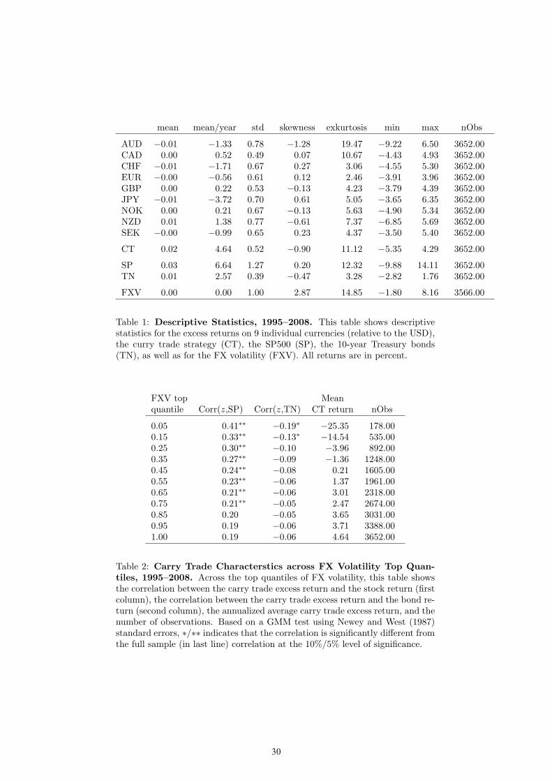
Table 1 (upper rows) contains summary statistics of the returns for the indi-

vidual G10 currencies. All returns have fat tails, most pronounced for the Aus-

tralian dollar. The average returns are negative for typical funding/borrowing

currencies (-3.7% for JPY and -1.7% for CHF, annualized) and positive for some

of the typical investment/lending currencies (1.4% for NZD, annualized).

3.2 Carry Trade Returns

A carry trade strategy consists of selling low interest rate currencies and buying

high interest rate currencies. To study typical carry trade strategies, we rely on

the explicit strategy followed by Deutsche Bank’s “PowerShares DB G10 Cur-

rency Harvest Fund”.6 It is based on the G10 currencies listed in the previous

subsection. The carry trade portfolio is composed of a long position in the three

currencies associated with the highest interest rates and a short position in the

three currencies with the lowest interest rates (cf. Gyntelberg and Remolona

(2007)). The portfolio is rebalanced every 3 months. We let rCTt denote the

return at time t on the carry trade strategy.

Table 1 (row 10) shows that the average carry trade return is higher than

for any individual currency and that the standard deviation is lower than for

all except one currency (i.e. CAD). This might explain the popularity of the

6More information about this index is available at the Deutsche Bank home page atwww.dbfunds.db.com.

9

strategy. As in Brunnermeier et al. (2009), we find that the distribution of

the return of the carry trade strategy is left skewed (i.e. the left tail of the

distribution is longer than the right tail), and that it has fat tails.

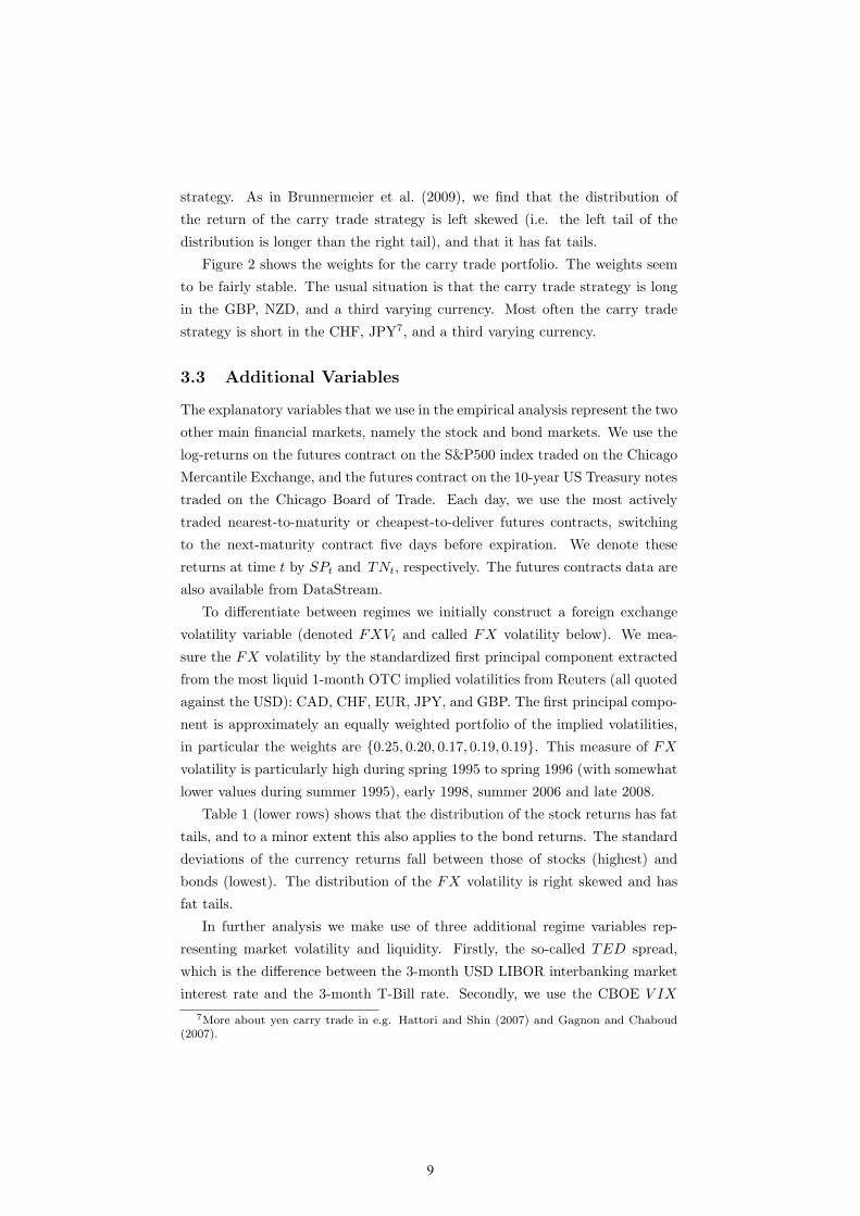
Figure 2 shows the weights for the carry trade portfolio. The weights seem

to be fairly stable. The usual situation is that the carry trade strategy is long

in the GBP, NZD, and a third varying currency. Most often the carry trade

strategy is short in the CHF, JPY7, and a third varying currency.

3.3 Additional Variables

The explanatory variables that we use in the empirical analysis represent the two

other main financial markets, namely the stock and bond markets. We use the

log-returns on the futures contract on the S&P500 index traded on the Chicago

Mercantile Exchange, and the futures contract on the 10-year US Treasury notes

traded on the Chicago Board of Trade. Each day, we use the most actively

traded nearest-to-maturity or cheapest-to-deliver futures contracts, switching

to the next-maturity contract five days before expiration. We denote these

returns at time t by SPt and TNt, respectively. The futures contracts data are

also available from DataStream.

To differentiate between regimes we initially construct a foreign exchange

volatility variable (denoted FXVt and called FX volatility below). We mea-

sure the FX volatility by the standardized first principal component extracted

from the most liquid 1-month OTC implied volatilities from Reuters (all quoted

against the USD): CAD, CHF, EUR, JPY, and GBP. The first principal compo-

nent is approximately an equally weighted portfolio of the implied volatilities,

in particular the weights are {0.25, 0.20, 0.17, 0.19, 0.19}. This measure of FX

volatility is particularly high during spring 1995 to spring 1996 (with somewhat

lower values during summer 1995), early 1998, summer 2006 and late 2008.

Table 1 (lower rows) shows that the distribution of the stock returns has fat

tails, and to a minor extent this also applies to the bond returns. The standard

deviations of the currency returns fall between those of stocks (highest) and

bonds (lowest). The distribution of the FX volatility is right skewed and has

fat tails.

In further analysis we make use of three additional regime variables rep-

resenting market volatility and liquidity. Firstly, the so-called TED spread,

which is the difference between the 3-month USD LIBOR interbanking market

interest rate and the 3-month T-Bill rate. Secondly, we use the CBOE V IX

7More about yen carry trade in e.g. Hattori and Shin (2007) and Gagnon and Chaboud(2007).

10

index, which is the index of implied volatilities on S&P500 stocks. Thirdly, we

measure market liquidity with the JPY/USD bid-ask spread computed as the

average of the ask price minus the bid price divided by their average at the end

of each five-minute interval during the day. We use the 10-day moving average

of the daily bid-ask spreads. We cap the spread at its 95% percentile to get rid

of the ten-fold increase on (fuzzy) holidays like Christmas.

Finally, we use the order flow for the JPY/USD as an additional explanatory

variable which is defined as the number of buys minus the number of sells during

the day (divided 10,000). Both the JPY/USD bid-ask spread and the order

flow are constructed from firm quotes and trading data obtained by the tick-by-

tick data of EBS (Electronic Broking Service). We only have JPY/USD data

covering the long sample period from 1997 to 2008. However, the JPY/USD is

notoriously considered the exchange rate subjected to most carry trade, so it

provides an interesting proxy.

4 Empirical Results

In this section we present the empirical results. First, we provide some pre-

liminary findings that further motivate the econometric framework. Then, we

show the empirical results for carry trade strategies as well as for the individual

currencies.

4.1 Preliminary Results

The return on the carry trade strategy is positively correlated with the return

on the stock market (0.19) and somewhat negatively correlated with the return

on the bond market (−0.06). This means that “investment currencies” like NZD

(the long positions of the carry trade strategy) tend to appreciate relative to

“funding currencies” like JPY and CHF (the short positions) when the stock

market booms. Conversely, investment currencies tend to depreciate against

funding currencies when bond prices increase (interest rates decrease). That is,

when the risk appetite of investors decrease and they move to safe assets (US

Treasury bonds are typically considered to be “safe havens”), then investment

currencies lose value against funding currencies.

While these patterns are already relatively well understood (see, for instance,

Bhansali (2007)), it is less well known that the strength of the correlations

depends very much on the level of FX market volatility and liquidity. As an

illustration, Table 2 (first column) shows how the correlation between the carry

trade return and the SP varies across the top quantiles of FX volatility. The

11

figure 0.41 is the correlation between the carry trade return and the SP return

for days when FX volatility is in the top 5%. The table shows a very clear

pattern, the higher the FX volatility, the stronger is the correlation between

the stock market and the carry trade strategy. In fact, the correlation coefficients

between the stock market and the carry trade strategy for the eight top volatility

quantiles are significantly higher than the correlation coefficient for the entire

sample (GMM based inference).

Similarly, Table 2 (second column) shows the correlations between the carry

trade return and TN at various top quantiles for the FX volatility. This corre-

lation is negative and numerically stronger for higher FX volatility—although

only the correlation coefficient at the two top most volatility quantiles are sig-

nificantly stronger than for the entire sample.

These preliminary results suggest that the risk exposures of the carry trade

strategy are much stronger during volatile periods than during calm periods.8

Table 2 (third column) reports the average returns of the carry trade strat-

egy for different top quantiles of FX volatility. On average, the carry trade

strategy yields positive and moderately high returns in normal periods, whereas

on average it has dramatic losses during turbulent periods.

4.2 Carry Trade Strategy

The preliminary findings suggest that both the risk exposure of the carry trade

return—as well the average carry trade return over short subsamples—are re-

lated to volatility of the FX markets. We now formalize this idea by using

a linear factor model (with stocks and bonds as factors), but where the betas

and the alpha (the intercept) depend on the one-day lagged FX volatility—

according to the logistic smooth transition regression model discussed above.

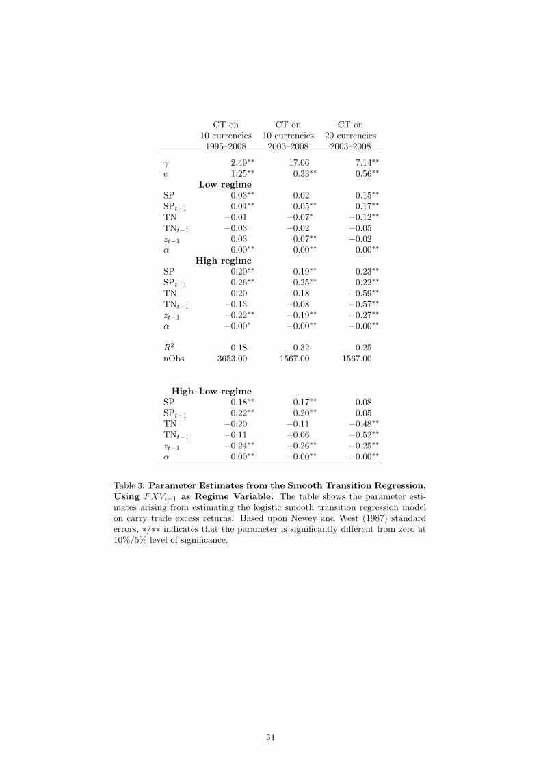
Table 3 (first column) shows the results from estimating the logistic smooth

transition regression model for the carry trade strategy. (The results in the

last two columns are discussed later.) The top part of the table shows the

parameter estimates applicable for low values of the FX volatility, denoted β1

in (3), and the middle part of the table shows the parameter estimates applicable

for high values of FX volatility, denoted β2. The lower part of the table shows

the difference between the parameter estimates for high and low FX volatility

values, i.e. it shows β2 − β1. Moreover, the table indicates whether these

differences are statistically significant.

The explanatory power of the smooth transition regression model is fairly

8However, the results should be read with appropriate reservations as Embrechts, McNeiland Straumann (2002) call for caution when using correlations in risk management.

12

high: The R2 is 0.18. As a comparison, an OLS regression gives half of that—

which suggests that it is empirically important to account for regime changes

in order to describe the exchange rate movements. The estimated value of

the c parameter (the central location of the logistic function) is 1.25, and the

estimated γ parameter (the steepness) is 2.49, so the estimated logistic function

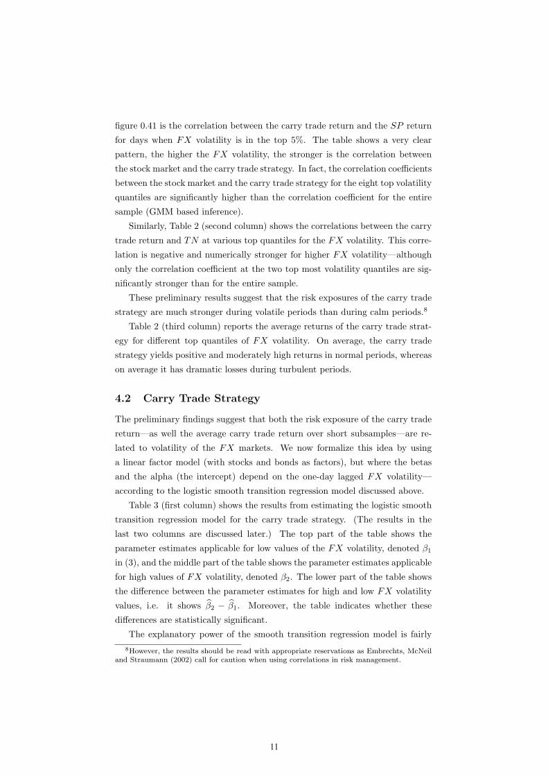
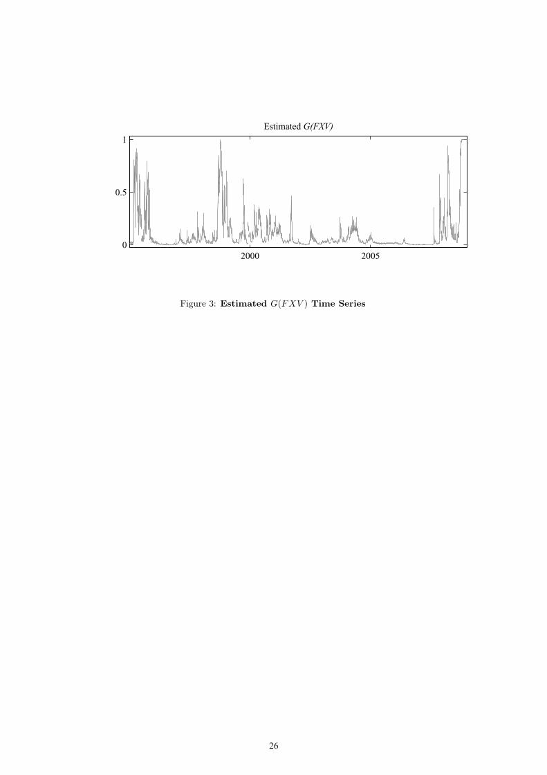
is similar to the solid curve in Figure 1 discussed above. In practice, this means

that the volatile regime starts to have an impact when the standardized FX

volatility variable goes above 1 or so. The resulting time path of G(FXV ) is

shown in Figure 3. The value is close to zero most of the time (it is less than

0.1 on 80% of the days in the sample) and it only occasionally goes above a half

(6% of the days). The calm regime (when β1 is the effective slope coefficient)

is thus the normal market situation, while the volatile regime (when β2, or a

weighted sum of β1 and β2, is the effective slope) represents periods of extreme

stress on the FX market.

The results in Table 3 clearly show that the risk exposure depends on the

FX volatility variable. During calm periods, the carry trade strategy is sig-

nificantly positively exposed to current and lagged stock returns (although the

coefficient is numerically small), but not to the bond market (a numerically

small, negative, coefficient). During turmoil, the exposure to the current and

lagged stock market returns is much larger. The exposure to the bond market

also has a more negative coefficient, but the difference between the regimes is

not significant. It is also interesting to note that the autoregressive component

is small and insignificant during calm periods, but significantly negative during

turmoil—which indicates considerable predictability and mean reversion during

volatile periods.

These results are robust to various changes in the empirical specification.

First, we replace the SP with the MSCI world index denominated in domestic

currencies and excluding US stocks. We get similar results. In particular, the

exposure to equity in the high volatility regime remains very high.9 Thus,

the carry trade’s exposure to stock market return appears irrespective of the

currency denomination and country of origin of the companies’ returns. Second,

taking into account transaction costs affects the average returns of the strategy

(decreasing it by 1.12 percentage points per year), but does not change any

of the slope coefficients.10 The main reason is that the trading costs are fairly

9Summing the contemporaneous and lagged coefficients gives 0.06 (0.52) for SP in the low(high) regime, -0.01 (-0.16) for TN and 0.03 (-0.16) for the lagged dependent variable.

10For each daily return we subtract 1/63 of half the bid-ask spread (in DataStream) fromthe beginning of the investment period (rebalancing every 3 months) and half of the bid-askspread from the end of the period. Since our return data is based on mid-quotes, this impliesthat the adjusted return is calculated from buying high and selling low.

13

stable over time and that there is little rebalancing (see Figure 2) as the interest

rate differentials are very persistent. Third, rebalancing the carry trade portfolio

more/less often than every three months does not change the qualitative results.

The main reason is that interest rates tend to change smoothly across time and

so do portfolio weights. The results are also robust to the number of long and

short currency positions in the carry trade strategy.11

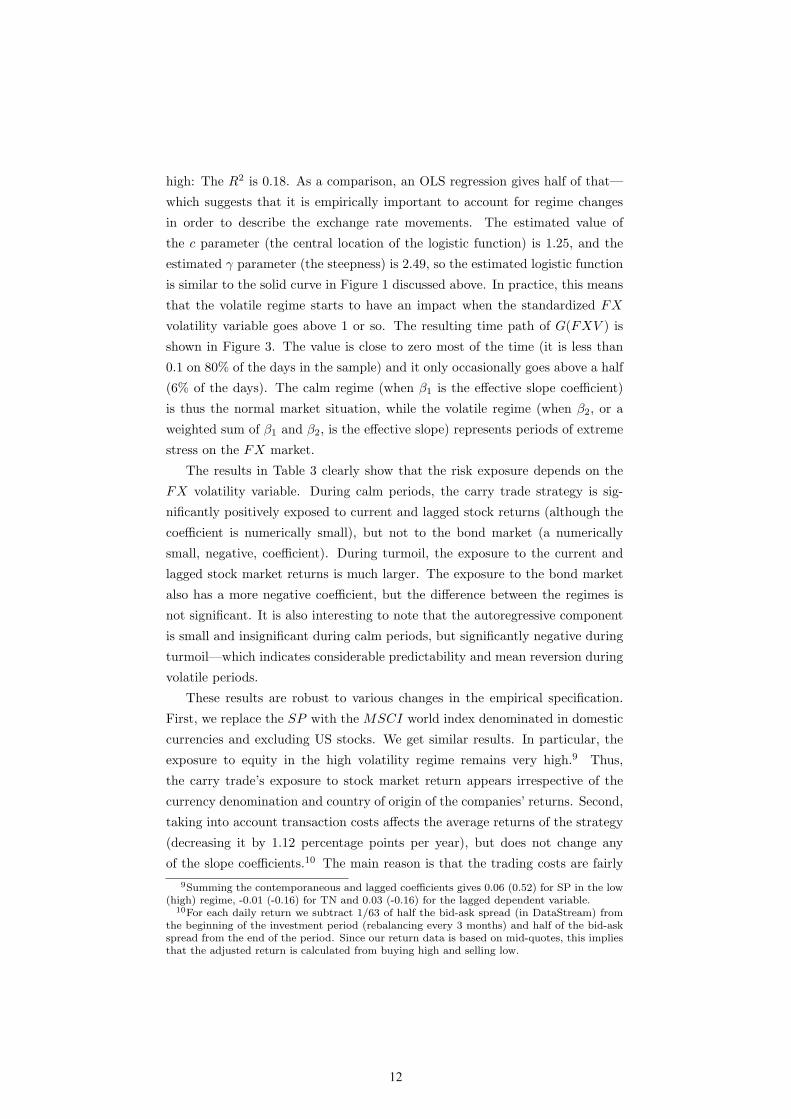
To assess the economic importance of the systematic risk of the carry trade

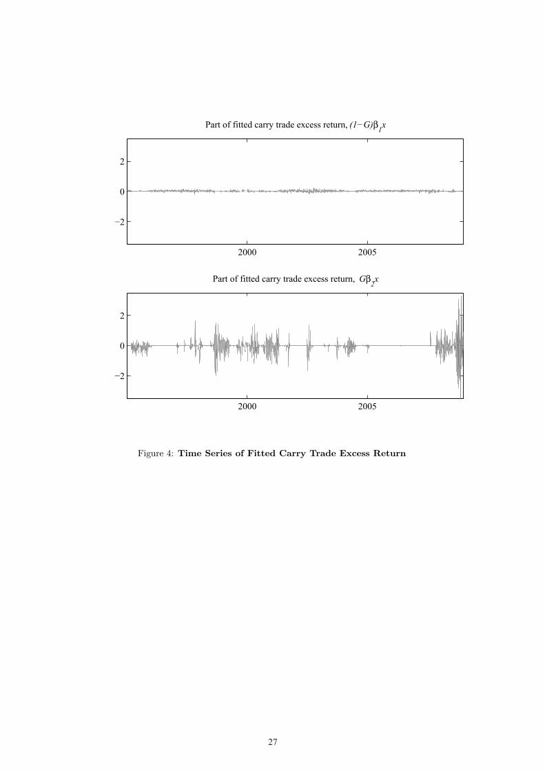
strategy we consider the fitted values (CT returns) in Figures 4–5. Figure

4 shows the fitted carry trade returns split up into two parts: the first part

(upper graph) caused by the calm regime ((1−G) β1xt) and the second part

(lower graph) caused by the volatile regime (Gβ2xt). The total fitted carry

trade return adds up to the sum of the two parts. Almost all the movement

in the fitted carry trade returns is caused by the volatile regime. So, it is

during volatile FX markets that the systematic risk of the carry trade is most

important. This is related to the literature that discusses whether financial

markets comovement is stronger during financial crises (cf. Forbes and Rigobon

(2002) and Corsetti, Pericoli and Sbracia (2005)) and also to the literature on

non-linearities and regime-dependence of carry trade returns (cf. Plantin and

Shin (2008) and Mark (1988)).

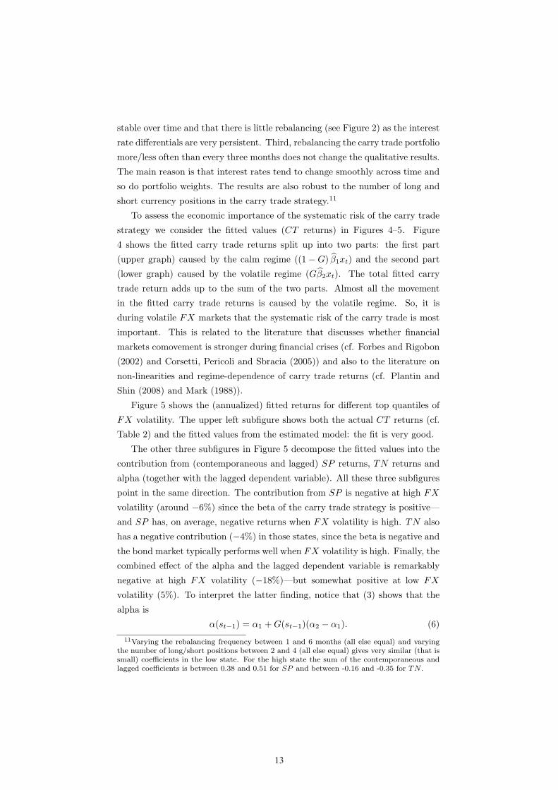
Figure 5 shows the (annualized) fitted returns for different top quantiles of

FX volatility. The upper left subfigure shows both the actual CT returns (cf.

Table 2) and the fitted values from the estimated model: the fit is very good.

The other three subfigures in Figure 5 decompose the fitted values into the

contribution from (contemporaneous and lagged) SP returns, TN returns and

alpha (together with the lagged dependent variable). All these three subfigures

point in the same direction. The contribution from SP is negative at high FX

volatility (around −6%) since the beta of the carry trade strategy is positive—

and SP has, on average, negative returns when FX volatility is high. TN also

has a negative contribution (−4%) in those states, since the beta is negative and

the bond market typically performs well when FX volatility is high. Finally, the

combined effect of the alpha and the lagged dependent variable is remarkably

negative at high FX volatility (−18%)—but somewhat positive at low FX

volatility (5%). To interpret the latter finding, notice that (3) shows that the

alpha is

α(st−1) = α1 +G(st−1)(α2 − α1). (6)

11Varying the rebalancing frequency between 1 and 6 months (all else equal) and varyingthe number of long/short positions between 2 and 4 (all else equal) gives very similar (that issmall) coefficients in the low state. For the high state the sum of the contemporaneous andlagged coefficients is between 0.38 and 0.51 for SP and between -0.16 and -0.35 for TN .

14

Since low volatility is the typical state, we can interpret α1 (positive) as the

typical alpha—and α2−α1 (negative) as the direct effect of high volatility on the

on the carry trade return. This is similar to Bhansali (2007) and Menkhoff et al.

(2009) who discuss how carry trades are negatively affected by market volatility.

Notice, however, that the alphas should not be taken as literal performance

measures since some of the factors are managed portfolios. (We do a formal

asset pricing test below.)

It can also be noticed that both the effect of the lagged dependent variable

and the direct FX volatility effect imply a certain amount of predictability (as

the state variable is measured in t− 1). We leave this aspect to future research.

To sum up, our results show that around one third of the (disastrous) carry

trade return in the (extreme) high volatility state is accounted for by the expo-

sure to traditional risk factors (equity and bonds) and two thirds by the market

volatility factor. This suggests that it is important to model both regime depen-

dence of traditional risk factors (see, for instance, McCurdy and Morgan (1991),

Dahlquist and Bansal (2000)) as well as the direct effect of market volatility on

carry trade performance (see, for instance, Bhansali (2007), Lustig et al. (2008)

and Menkhoff et al. (2009)).

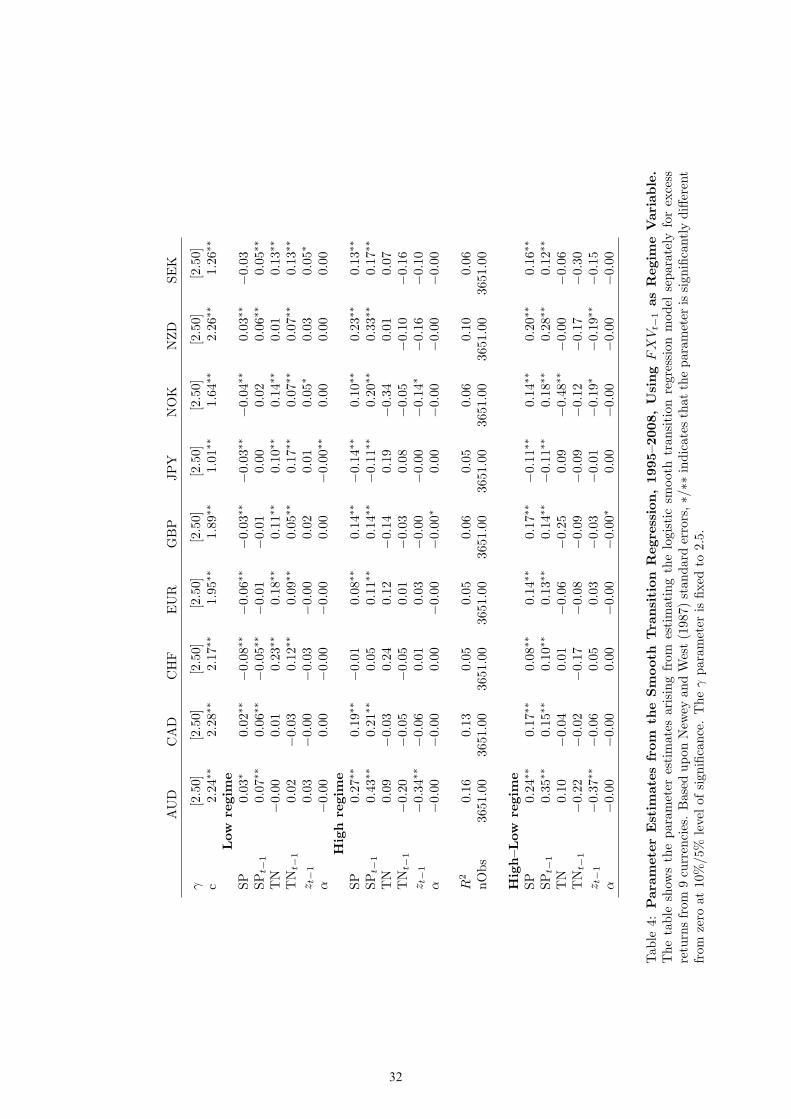
4.3 Individual Currencies

Table 4 shows the results from estimating the logistic smooth transition regres-

sion model for the individual currency returns. In these regressions, we set γ

equal to 2.50 to guarantee a unique and consistent number across the panel

(the point estimate for the carry trade return is 2.49). The table is structured

similarly to Table 3. The results for the individual currencies are broadly in line

with those from the carry trade. In both regimes, typical investment currencies

like NZD have positive exposure to SP , while typical funding currencies like

CHF and JPY have negative SP risk exposure (a safe haven feature). In most

cases, this pattern is even stronger in the high volatility regime (the change

in the slope coefficient is significant for all currencies). Together this explains

why the carry trade is so strongly exposed to SP risk, particularly in the high

volatility regime. In addition, the negative autocorrelation in the carry trade

strategy in the high volatility regime seems to be driven by the typical invest-

ment currencies.

15

4.4 Larger Set of Currencies

Constructing the carry trade strategy from a larger base of 20 currencies (also

called G20) instead of 10 currencies does not alter the conclusion. To show that,

Table 3 also reports results for a carry trade strategy based on the G10 currencies

for the shorter sample 2003–2008 (instead of the 1995–2008 sample discussed

above) and for a strategy based on the G10 and 10 additional currencies (also

for 2003–2008). The sample starts in 2003 in order to guarantee high quality

data and the existence of an active carry trade market.

The results for the larger set of currencies base are very much in line with

those for the G10 currencies—and perhaps even stronger. In particular, the

negative exposure to the bond market is stronger (and more significant).

Accounting for the transaction costs decreases the carry trade performance

by 1 percentage point per year, but does not affect the slope coefficients—as

in the G10 case. Although the trading costs are higher for these additional 10

currencies, there is less rebalancing since some of the interest rate differentials

are extremely persistent. Overall this leads to almost the same adjustment of

the average performance as in the G10 case.

4.5 Asset Pricing Analysis

These regime-dependent risk exposures have important implications for the

cross-sectional fit of the model. To illustrate this, we estimate a simplified

model with the following specification: (i) the factors (ft) are only contempora-

neous variables; (ii) SP and TN are expressed as excess returns over a risk-free

US interest rate; and (iii) the parameters of the logistic function are fixed (at

the values estimated from the carry trade return).

By these simplifications, the model becomes testable (sufficient number of

test assets compared to factors) and is a linear factor model with the following

factors

ft = [SPt, TNt, Gt−1 × SPt, Gt−1 × TNt, Gt−1]. (7)

Since some of the factors are not excess returns, the asset pricing implications

are tested by studying whether the cross-sectional variation in average returns

is explained by the betas of the factors

∑T

t=1rt/T = β′λ, (8)

where λ is a vector of factor risk premia. The model is estimated by GMM

where the first set of moment conditions effectively estimate the betas (and an

16

intercept) by regressing each currency return on the factors (time-series regres-

sions) and the second set of moment conditions estimate the factor risk premia

by a cross-sectional regression. We discipline the exercise by using the fact that

the SP and TN are excess returns: these factors are included in the vector of

test assets (together with the currencies) and formulate the moment conditions

so that the factor risk premia for these two factors are just their average returns.

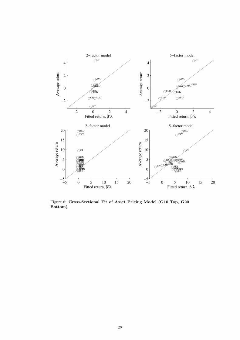
Figure 6 (upper panel) compares the results from using just SP and TN (a 2-

factor model) with those from using all 5 factors in (7) for the G10 sample. While

the 2-factor model explains virtually nothing of the cross-sectional variation of

the currency returns, the 5-factor model is much more successful. For instance,

the low return on JPY is well explained—mostly by the negative exposure to

equity in the high volatility state. Similarly, the pricing error (the vertical

distance to the 45 degree line) for the carry trade strategy (marked by CT ) is

substantially smaller in the 5-factor model, although it is not zero. Because of

the few degrees of freedom, the power of formal tests of the model is low.

The lower panel of Figure 6 shows the asset implication for the 20 currencies

and the corresponding carry trade strategy (CT ). As before, the 2-factor ex-

plains almost nothing of the cross-sectional variation of average returns, while

the 5-factor works clearly better. In contrast to before, the formal test of the

overidentifying restrictions has enough degrees of freedom to discriminate be-

tween the models: the 2-factor model is rejected on the 2% significance level,

while the 5-factor cannot be rejected even on the 20% significant level. It is

also interesting to notice that the pricing error of the carry trade strategy is

virtually zero in the 5-factor model (but almost 10% in the 2-factor model).

Overall, this gives considerable support for a model with regime-dependent

risk exposures.

4.6 Other Regime Variables

So far, we have related the regime mechanism to a measure of risk on exchange

rate markets. Here, we extend our analysis to more general proxies of global risk

or risk aversion (the V IX, as used by Lustig et al. (2008) and Menkhoff et al.

(2009)), of funding liquidity (the TED, as in Brunnermeier et al. (2009)) as well

as market liquidity. To capture the latter, we use the JPY/USD bid-ask daily

spread as a measure of transaction cost due to market illiquidity (Roll (1984))

and asymmetric information (Glosten and Milgrom (1985)). It should be noted

that since we use EBS data, this measure accounts only for inter-dealer and

brokered FX spot trading and not other trading venues such as OTC markets.

Using these other natural candidates for the regime variable does not change

17

the results much. Table 5 shows the smooth transition regressions for the carry

trade strategy for the sample 1997–2008 for different choices of the regime vari-

able. The sample starts in 1997 (instead of 1995) due to limited data availability

for some of the new regime variables. For convenience, the first column of the

table uses the same specification as before: the FX volatility (FXV ; now for

the shorter sample period).

The second column uses the TED spread, the third the V IX index, and

the fourth the JPY/USD bid-ask spread. The results are similar across these

different specifications.

The last column reports results from a regression where we use all four state

variables simultaneously. Both the FXV and the TED are highly significant,

while the V IX and bid-ask spread are not. (In this regression the state regime

variables are rotated to be uncorrelated, but we get a similar result with the

original variables.)

The correlations between these different regime variables are reasonably high

(0.4–0.75), suggesting a well-expected co-variation between risk and illiquidity

(of any nature).12 Not surprisingly, the different regimes variables generate

fairly similar results for the time variation in risk exposure. However, a direct

horse race favors the FX volatility and the TED over V IX and the bid-ask

spread.

These findings suggest that FX market volatility and funding liquidity might

be more important than risk measures related to equity markets (V IX) and

direct measures of FX (inter-dealer) market liquidity (bid-ask spread). This

is somewhat similar to the findings on the equity market by Bandi, Moise and

Russell (2008).

4.7 Further Robustness Analysis

4.7.1 Longer Sample Period

It is of considerable interest to see if the properties of carry trade documented

above (on data 1995–2008) also hold for earlier periods—especially during pe-

riods of FX market turmoil. We therefore study also the sample 1976–2008,

but have to reduce the number of currencies under investigation to seven, be-

cause we cannot obtain high-quality interest rate data (for the early part of the

sample) for Norway, New Zealand, and Sweden.

For the longer sample period we have to define a new FX volatility variable,

since data on the FX options are not available before 1995. Instead we use a

12The lowest correlation is between TED and the bid-ask spread and the highest is betweenFX volatility and the bid-ask spread.

18

15-day moving average of the first principal component of the absolute value

of the FX daily returns (see Taylor (1986)). This new FX volatility variable

is backward looking and does not necessarily represent the beliefs of market

participants, but it is still a reasonable approximation. For instance, over the

1995–2008 sample the correlation with the option based measure is 0.85.

For this longer sample most coefficients are numerically small (cf. Burnside

et al. (2008) who find no relation between carry trade strategies and an equity

factor for the same time period). However, the exposure to equity in the high

volatility state is as strong as in the shorter sample (0.18 for the contempora-

neous coefficient and 0.21 for the lagged coefficient). The main findings from

the long sample and from the shorter sample are highly similar, except that the

bond factor is less important.

Overall, it seems as if the time-varying exposure to equity has been an

important feature during both earlier periods of FX market turbulence13 as

well as during more recent episodes14. This suggests that our findings cannot

be solely driven by the current financial crisis.

4.7.2 Effects of Order Flow

In the market microstructure literature, the order flow is often thought of as

representing the net demand pressure (Evans and Lyons (2002)). To investigate

the importance of this in our model, Table 6 shows logistic smooth transition

regressions for the Japanese yen (against the USD) for the sample 1997–2008,

with and without controlling for order flow.

The results for the standard specification are very similar to those reported

before (but for the sample 1995–2008): the yen appears to be a safe haven asset

(the betas have the opposite sign compared to the carry trade strategy). The

second column includes one more regressor: the order flow on the JPY/USD

exchange rate, measured as the number of buyer-initiated trades minus the

number of seller-initiated trades (where a trade means buying JPY and selling

USD). The coefficient related to the order flow is significantly positive, so there

is a significant price impact meaning that demand pressure is associated with a

currency appreciation, as expected. More importantly for our paper, however,

is the fact that including the order flow does not materially change the betas

on the equity and bond markets.

13For instance, the global credit crunch preventing several developing countries from payingtheir debt in 1982, the bond and equity market crashes in 1987 and the burst of the Japanesebubble together with the junk bond crisis in 1989 and the French Maastricht Treaty thatsparked crisis in European Monetary System in 1992.

14For instance, Asian financial crisis in 1997-8 and the recent financial crisis in 2007-8.

19

Although limited to the JPY/USD exchange rate, this finding still suggests

that our previous conclusions on the time-varying risk exposure are not sensitive

to the inclusion/exclusion of order flow.

5 Conclusion

This paper studies the risk exposure of carry trade returns by estimating factor

models on daily data from 1995 to 2008. The risk factors are traditional (equity

and bond returns), but the risk exposures are allowed to depend on proxies for

volatility and (market and funding) liquidity. We also allow for mean-reversion

and use the volatility and risk proxies as additional factors.

The results from carry trade strategies based on the G10 currencies show

that carry trade returns have highly regime-dependent risk exposures: the beta

related to the stock market is positive in normal times—and much more so

during turbulent times. In addition, the returns are more predictable (mean-

reverting) during turmoil and have a direct exposure to a volatility factor. The

results also hold for individual currencies: typical investment currencies have a

positive exposure to equities and this exposure is much larger during periods

of FX market turmoil, while typical funding currencies are the mirror image.

The results are robust to applying of a larger set of currencies including emerg-

ing market currencies, longer sample periods, other definitions of stock market

returns, net of transaction costs, and after controlling for order flow.

The economic importance of the results is significant. For instance, the

(abysmal) performance of carry trade strategies during times of high (extreme)

market volatility is by one third driven by exposure to traditional risk factors

(equity and bond returns) and by two thirds by exposure to the volatility factor

itself. Moreover, the regime-dependent factor model assigns a very small pricing

error to the carry trade strategy—in stark contrast to a traditional factor model,

which suggests a zero risk premium for the strategy.

We tested several variables in order to determine which factors govern the

regime-dependency of the systematic risk inherent to the carry trade strategies.

We find that FX market volatility and funding liquidity (the TED spread)

are more relevant than measures of equity market volatility and risk aversion

(V IX) or the FX market liquidity (bid-ask spread).

Our findings provide further evidence on the recent research showing that

financial markets are regime-dependent with stronger comovements during fi-

nancial crises (Plantin and Shin (2008), Forbes and Rigobon (2002) and Corsetti

et al. (2005)), and that volatility and liquidity have important direct effects on

20

asset returns (Acharya and Pedersen (2005), Ang et al. (2006) and Bhansali

(2007)). Our results also indicate that carry trade looks less attractive once

correctly priced by means of regime-dependent models—suggesting a partial

resolution of the UIP puzzle.

21

References

Acharya, V. V. and Pedersen, L. H.: 2005, Asset pricing with liquidity risk,

Journal of Financial Economics 77(2), 375–410.

Ang, A., Hodrick, R. J., Xing, Y. and Zhang, X.: 2006, The cross-section of

volatility and expected returns, Journal of Finance 61(1), 259–299.

Bacchetta, P. and van Wincoop, E.: 2006, Can information heterogeneity ex-

plain the exchange rate determination puzzle?, American Economic Review

96, 552–576.

Bandi, F. M., Moise, C. E. and Russell, J. R.: 2008, The joint pricing of volatility

and liquidity. mimeo, University of Chicago.

Bekaert, G. and Gray, S. F.: 1998, Target zones and exchange rates: an empirical

investigation, Journal of International Economics 45, 1–35.

Bhansali, V.: 2007, Volatility and the carry trade, Journal of Fixed Income

17(3), 72–84.

Brunnermeier, M., Nagel, S. and Pedersen, L.: 2009, Carry trades and currency

crashes, NBER Macroeconomics Annual 2008 23, 313–347.

Burnside, C., Eichenbaum, M., Kleshchelski, I. and Rebelo, S.: 2008, Can peso

problems explain the returns to the carry trade?, Working Paper 14054,

NBER.

Burnside, C., Eichenbaum, M. and Rebelo, S.: 2007, The returns to currency

speculation in emerging markets, American Economic Review 97(2), 333–

338.

Corsetti, G., Pericoli, M. and Sbracia, M.: 2005, Some contagion, some in-

terdependence: more pitfalls in tests of financial contagion, Journal of

International Money and Finance 24(8), 1177–1199.

Dahlquist, M. and Bansal, R.: 2000, The forward premium puzzle: different

tales from developed and emerging economies, Journal of International

Economics 51, 115–144.

Dumas, B.: 1992, Dynamic equilibrium and the real exchange rate in a spatially

separated world, Review of Financial Studies 5(2), 153–180.

Embrechts, P., McNeil, A. and Straumann, D.: 2002, Correlation and depen-

dence in risk management: properties and pitfalls, in M. Dempster (ed.),

22

Risk Management: Value at Risk and Beyond, Cambridge University Press,

Cambridge, pp. 176–223.

Evans, M. D. and Lyons, R. K.: 2002, Order flow and exchange rate dynamics,

Journal of Political Economy 110(1), 170–180.

Fama, E. F.: 1984, Forward and spot exchange rates, Journal of Monetary

Economics 14(3), 319–338.

Farhi, E. and Gabaix, X.: 2008, Rare disasters and exchange rates, Working

paper, Harvard University and NYU Stern.

Forbes, K. J. and Rigobon, R.: 2002, No contagion, only interdependence: mea-

suring stock market comovements, Journal of Finance 57(5), 2223–2261.

Gagnon, J. E. and Chaboud, A.: 2007, What can the data tell us about carry

trades in japanese yen?, International Finance Discussion Paper 899, Fed-

eral Reserve Bank.

Glosten, L. R. and Milgrom, P. R.: 1985, Bid, ask and transaction prices in

a specialist market with heterogeneously informed traders, Journal of Fi-

nancial Economics 14(1), 71–100.

Gyntelberg, J. and Remolona, E. M.: 2007, Risk in carry trade: A look at target

currencies in asia and the pacific, BIS Quarterly Review (December), 73–82.

Hattori, M. and Shin, H. S.: 2007, The broad yen carry trade, Working paper,

Bank of Japan.

Ichiue, H. and Koyama, K.: 2008, Regime switches in exchange rate volatility

and uncovered interest parity, Working paper, Bank of Japan.

Krugman, P.: 1991, Target zones and exchange rate dynamics, Quarterly Jour-

nal of Economics 106, 669–682.

Lustig, H., Roussanov, N. and Verdelhan, A.: 2008, Common risk factors in

currency markets, Working Paper 14082, NBER.

Lyons, R. K.: 2001, The microstructure approach to exchange rates, MIT Press,

Cambridge, Massachusetts.

Mark, N. C.: 1988, Time-varying betas and risk premia in the pricing of forward

exchange contracts, Journal of Financial Economics 22, 335–354.

23

McCurdy, T. H. and Morgan, I. G.: 1991, Tests for a systematic risk compo-

nent in deviations from uncovered interest rate parity, Review of Economic

Studies 58(3), 587–602.

Menkhoff, L., Sarno, L., Schmeling, M. and Schrimpf, A.: 2009, Carry trades

and global foreign exchange volatility. mimeo, Leibniz Universitaet Han-

nover.

Newey, W. K. and West, K. D.: 1987, A simple, positive semi-definite, het-

eroskedasticity and autocorrelation consistent covariance matrix, Econo-

metrica 55(3), 703–708.

Plantin, G. and Shin, H. S.: 2008, Carry trades and speculative dynamics,

Working paper, London Business School and Princeton University.

Roll, R.: 1984, A simple implicit measure of the effective bid-ask spread in an

efficient market, Journal of Finance 39(4), 1127–1139.

Sarno, L., Valente, G. and Leon, H.: 2006, Nonlinearity in deviations from

uncovered interest parity: an explanation of the forward bias puzzle, Review

of Finance 10(3), 443–482.

Taylor, S.: 1986, Modeling Financial Time Series, Wiley.

van Dijk, D., Tersvirta, T. and Franses, P. H.: 2002, Smooth transition autore-

gressive models - a survey of recent developments, Econometric Reviews

21(1), 1–47.

24

−0.5 0 0.5 1 1.5 2 2.5

β1

β2

s

Effective coefficient of xt for different G functions

c = 1.2, γ = 2.5c = 0.5, γ = 2.5c = 1.2, γ = 5

Figure 1: Example of Smooth Transition Regression Model

25

2000 2005−1/3

0

1/3AUD

2000 2005−1/3

0

1/3CAD

2000 2005−1/3

0

1/3CHF

2000 2005−1/3

0

1/3EUR

2000 2005−1/3

0

1/3GBP

2000 2005−1/3

0

1/3JPY

2000 2005−1/3

0

1/3NOK

2000 2005−1/3

0

1/3NZD

2000 2005−1/3

0

1/3SEK

2000 2005−1/3

0

1/3USD

Figure 2: Carry Trade Strategy Weights

26

2000 20050

0.5

1Estimated G(FXV)

Figure 3: Estimated G(FXV ) Time Series

27

2000 2005

−2

0

2

Part of fitted carry trade excess return, (1−G)β1x

2000 2005

−2

0

2

Part of fitted carry trade excess return, Gβ2x

Figure 4: Time Series of Fitted Carry Trade Excess Return

28

00.51−40

−20

0

20Mean carry trade return

Top quantile of FXV

ActualFitted

00.51−10

−5

0

5Fitted CT return, S&P contribution

Top quantile of FXV

00.51−4

−2

0Fitted CT return, TN contribution

Top quantile of FXV00.51

−20

−10

0

10Fitted CT return, α & lag contribution

Top quantile of FXV

Figure 5: Fitted (Annualized) CT Returns for Different Top Quantilesof FX Volatility

29

−2 0 2 4

−2

0

2

4

2−factor model

Fitted return, β’λ

Ave

rage

ret

urn

AUD

CAD

CHF

EUR

GBP

JPY

NOK

NZD

SEK

CT

−2 0 2 4

−2

0

2

4

5−factor model

Fitted return, β’λ

Ave

rage

ret

urn

AUD

CAD

CHF

EUR

GBP

JPY

NOK

NZD

SEK

CT

−5 0 5 10 15 20−5

0

5

10

15

202−factor model

Fitted return, β’λ

Ave

rage

ret

urn

AUD

BRL

CAD

CHF

CZK

EUR

GBP

ILSINR

ISK

JPYMXNNOK

NZDPLNRUB

SEK

TRY

ZAR

CT

−5 0 5 10 15 20−5

0

5

10

15

205−factor model

Fitted return, β’λ

Ave

rage

ret

urn

AUD

BRL

CAD

CHF

CZK

EUR

GBP

ILSINR

ISK

JPYMXNNOK

NZDPLN

RUB

SEK

TRY

ZAR

CT

Figure 6: Cross-Sectional Fit of Asset Pricing Model (G10 Top, G20Bottom)

30

mean mean/year std skewness exkurtosis min max nObs

AUD −0.01 −1.33 0.78 −1.28 19.47 −9.22 6.50 3652.00CAD 0.00 0.52 0.49 0.07 10.67 −4.43 4.93 3652.00CHF −0.01 −1.71 0.67 0.27 3.06 −4.55 5.30 3652.00EUR −0.00 −0.56 0.61 0.12 2.46 −3.91 3.96 3652.00GBP 0.00 0.22 0.53 −0.13 4.23 −3.79 4.39 3652.00JPY −0.01 −3.72 0.70 0.61 5.05 −3.65 6.35 3652.00NOK 0.00 0.21 0.67 −0.13 5.63 −4.90 5.34 3652.00NZD 0.01 1.38 0.77 −0.61 7.37 −6.85 5.69 3652.00SEK −0.00 −0.99 0.65 0.23 4.37 −3.50 5.40 3652.00

CT 0.02 4.64 0.52 −0.90 11.12 −5.35 4.29 3652.00

SP 0.03 6.64 1.27 0.20 12.32 −9.88 14.11 3652.00TN 0.01 2.57 0.39 −0.47 3.28 −2.82 1.76 3652.00

FXV 0.00 0.00 1.00 2.87 14.85 −1.80 8.16 3566.00

Table 1: Descriptive Statistics, 1995–2008. This table shows descriptivestatistics for the excess returns on 9 individual currencies (relative to the USD),the curry trade strategy (CT), the SP500 (SP), the 10-year Treasury bonds(TN), as well as for the FX volatility (FXV). All returns are in percent.

FXV top Meanquantile Corr(z,SP) Corr(z,TN) CT return nObs

0.05 0.41∗∗ −0.19∗ −25.35 178.000.15 0.33∗∗ −0.13∗ −14.54 535.000.25 0.30∗∗ −0.10 −3.96 892.000.35 0.27∗∗ −0.09 −1.36 1248.000.45 0.24∗∗ −0.08 0.21 1605.000.55 0.23∗∗ −0.06 1.37 1961.000.65 0.21∗∗ −0.06 3.01 2318.000.75 0.21∗∗ −0.05 2.47 2674.000.85 0.20 −0.05 3.65 3031.000.95 0.19 −0.06 3.71 3388.001.00 0.19 −0.06 4.64 3652.00

Table 2: Carry Trade Characterstics across FX Volatility Top Quan-tiles, 1995–2008. Across the top quantiles of FX volatility, this table showsthe correlation between the carry trade excess return and the stock return (firstcolumn), the correlation between the carry trade excess return and the bond re-turn (second column), the annualized average carry trade excess return, and thenumber of observations. Based on a GMM test using Newey and West (1987)standard errors, ∗/∗∗ indicates that the correlation is significantly different fromthe full sample (in last line) correlation at the 10%/5% level of significance.

31

CT on CT on CT on10 currencies 10 currencies 20 currencies1995–2008 2003–2008 2003–2008

γ 2.49∗∗ 17.06 7.14∗∗

c 1.25∗∗ 0.33∗∗ 0.56∗∗

Low regimeSP 0.03∗∗ 0.02 0.15∗∗

SPt−1 0.04∗∗ 0.05∗∗ 0.17∗∗

TN −0.01 −0.07∗ −0.12∗∗

TNt−1 −0.03 −0.02 −0.05zt−1 0.03 0.07∗∗ −0.02α 0.00∗∗ 0.00∗∗ 0.00∗∗

High regimeSP 0.20∗∗ 0.19∗∗ 0.23∗∗

SPt−1 0.26∗∗ 0.25∗∗ 0.22∗∗

TN −0.20 −0.18 −0.59∗∗

TNt−1 −0.13 −0.08 −0.57∗∗

zt−1 −0.22∗∗ −0.19∗∗ −0.27∗∗

α −0.00∗ −0.00∗∗ −0.00∗∗

R2 0.18 0.32 0.25nObs 3653.00 1567.00 1567.00

High–Low regimeSP 0.18∗∗ 0.17∗∗ 0.08SPt−1 0.22∗∗ 0.20∗∗ 0.05TN −0.20 −0.11 −0.48∗∗

TNt−1 −0.11 −0.06 −0.52∗∗

zt−1 −0.24∗∗ −0.26∗∗ −0.25∗∗

α −0.00∗∗ −0.00∗∗ −0.00∗∗

Table 3: Parameter Estimates from the Smooth Transition Regression,Using FXVt−1 as Regime Variable. The table shows the parameter esti-mates arising from estimating the logistic smooth transition regression modelon carry trade excess returns. Based upon Newey and West (1987) standarderrors, ∗/∗∗ indicates that the parameter is significantly different from zero at10%/5% level of significance.

32

AUD

CAD

CHF

EUR

GBP

JPY

NOK

NZD

SEK

γ[2.50]

[2.50]

[2.50]

[2.50]

[2.50]

[2.50]

[2.50]

[2.50]

[2.50]

c2.24∗∗

2.28∗∗

2.17∗∗

1.95∗∗

1.89∗∗

1.01∗∗

1.64∗∗

2.26∗∗

1.26∗∗

Low

regim

eSP

0.03∗

0.02∗∗

−0.08∗∗

−0.06∗∗

−0.03∗∗

−0.03∗∗

−0.04∗∗

0.03∗∗

−0.03

SPt−

10.07∗∗

0.06∗∗

−0.05∗∗

−0.01

−0.01

0.00

0.02

0.06∗∗

0.05∗∗

TN

−0.00

0.01

0.23∗∗

0.18∗∗

0.11∗∗

0.10∗∗

0.14∗∗

0.01

0.13∗∗

TN

t−1

0.02

−0.03

0.12∗∗

0.09∗∗

0.05∗∗

0.17∗∗

0.07∗∗

0.07∗∗

0.13∗∗

z t−1

0.03

−0.00

−0.03

−0.00

0.02

0.01

0.05∗

0.03

0.05∗

α−0

.00

0.00

−0.00

−0.00

0.00

−0.00∗∗

0.00

0.00

0.00

High

regim

eSP

0.27∗∗

0.19∗∗

−0.01

0.08∗∗

0.14∗∗

−0.14∗∗

0.10∗∗

0.23∗∗

0.13∗∗

SPt−

10.43∗∗

0.21∗∗

0.05

0.11∗∗

0.14∗∗

−0.11∗∗

0.20∗∗

0.33∗∗

0.17∗∗

TN

0.09

−0.03

0.24

0.12

−0.14

0.19

−0.34

0.01

0.07

TN

t−1

−0.20

−0.05

−0.05

0.01

−0.03

0.08

−0.05

−0.10

−0.16

z t−1

−0.34∗∗

−0.06

0.01

0.03

−0.00

−0.00

−0.14∗

−0.16

−0.10

α−0

.00

−0.00

0.00

−0.00

−0.00∗

0.00

−0.00

−0.00

−0.00

R2

0.16

0.13

0.05

0.05

0.06

0.05

0.06

0.10

0.06

nObs

3651.00

3651.00

3651.00

3651.00

3651.00

3651.00

3651.00

3651.00

3651.00

High–Low

regim

eSP

0.24∗∗

0.17∗∗

0.08∗∗

0.14∗∗

0.17∗∗

−0.11∗∗

0.14∗∗

0.20∗∗

0.16∗∗

SPt−

10.35∗∗

0.15∗∗

0.10∗∗

0.13∗∗

0.14∗∗

−0.11∗∗

0.18∗∗

0.28∗∗

0.12∗∗

TN

0.10

−0.04

0.01

−0.06

−0.25

0.09

−0.48∗∗

−0.00

−0.06

TN

t−1

−0.22

−0.02

−0.17

−0.08

−0.09

−0.09

−0.12

−0.17

−0.30

z t−1

−0.37∗∗

−0.06

0.05

0.03

−0.03

−0.01

−0.19∗

−0.19∗∗

−0.15

α−0

.00

−0.00

0.00

−0.00

−0.00∗

0.00

−0.00

−0.00

−0.00

Tab

le4:

Para

meterEstim

atesfrom

theSmooth

Tra

nsition

Regre

ssion,1995–2008,Using

FXVt−

1asRegim

eVariable.

Thetable

show

stheparameter

estimatesarisingfrom

estimatingthelogisticsm

oothtransitionregressionmodel

separately

forexcess

returnsfrom

9currencies.BaseduponNew

eyan

dWest(1987)standard

errors,∗/

∗∗indicatesthattheparameter

issignificantlydifferent

from

zero

at10%/5%

level

ofsignificance.Theγparameter

isfixed

to2.5.

33

Regime variable:

Bid-askFXV TED VIX spread All

γFXV 2.83∗∗ 1.68∗∗

γTED 1.86∗ 1.68∗∗

γV IX 11.84∗∗ 0.39γBA 2.38∗∗ −0.22c 1.19∗∗ 1.31∗∗ 2.35∗∗ 1.81∗∗ 0.81∗∗

Low regimeSP 0.03∗∗ 0.02 0.05∗∗ 0.04∗∗ 0.02∗

SPt−1 0.04∗∗ 0.04∗∗ 0.05∗∗ 0.06∗∗ 0.03∗∗

TN 0.00 0.05 −0.04 −0.03 0.04TNt−1 −0.03 −0.02 −0.05∗∗ −0.03 −0.02zt−1 0.02 0.04 −0.00 −0.02 0.03α 0.00∗∗ 0.00∗∗ 0.00∗∗ 0.00∗∗ 0.00∗∗

High regimeSP 0.20∗∗ 0.19∗∗ 0.19∗∗ 0.20∗∗ 0.19∗∗

SPt−1 0.25∗∗ 0.24∗∗ 0.26∗∗ 0.23∗∗ 0.24∗∗

TN −0.25 −0.35∗ −0.17 −0.15 −0.30∗

TNt−1 −0.09 −0.17 −0.10 −0.30 −0.13zt−1 −0.18∗∗ −0.20∗∗ −0.23∗∗ −0.11 −0.18∗∗

α 0.00∗∗ −0.00∗∗ −0.00∗∗ −0.00∗∗ −0.00∗∗

R2 0.21 0.22 0.20 0.18 0.23nObs 3132.00 3132.00 3132.00 3132.00 3132.00

High–Low regimeSP 0.17∗∗ 0.17∗∗ 0.14∗∗ 0.16∗∗ 0.17∗∗

SPt−1 0.21∗∗ 0.21∗∗ 0.20∗∗ 0.17∗∗ 0.21∗∗

TN −0.25 −0.40∗∗ −0.13 −0.12 −0.34∗

TNt−1 −0.06 −0.15 −0.05 −0.27 −0.11zt−1 0.20∗∗ −0.23∗∗ −0.23∗∗ −0.09 −0.21∗∗

α 0.00∗∗ −0.00∗∗ −0.00∗∗ −0.00∗∗ −0.00∗∗

Table 5: Parameter Estimates from the Smooth Transition Regres-sion, 1997–2008, Using Different Regime Variables. The table showsthe parameter estimates arising from estimating the logistic smooth transitionregression model on carry trade excess returns. Based upon Newey and West(1987) standard errors, ∗/∗∗ indicates that the parameter is significantly differ-ent from zero at 10%/5% level of significance.

34

Standard Withspecification Order flow

γ [2.5] [2.5]c 1.01∗∗ 0.91∗∗

Low regimeSP −0.03∗∗ −0.02SPt−1 0.01 0.01TN 0.11∗∗ 0.08∗∗

TNt−1 0.21∗∗ 0.20∗∗

Order flow 0.06∗∗

zt−1 −0.01 −0.00α −0.00∗∗ 0.00∗∗

High regimeSP −0.13∗∗ −0.11∗∗

SPt−1 −0.11∗∗ −0.10∗∗

TN 0.25 0.15TNt−1 0.11 0.11Order flow 0.07zt−1 0.03 0.02α 0.00 −0.00∗

R2 0.06 0.09nObs 3130.00 3130.00

High–Low regimeSP −0.11∗∗ −0.09∗∗

SPt−1 −0.11∗∗ −0.11∗∗

TN 0.14 0.06TNt−1 −0.10 −0.09Order flow 0.01zt−1 0.04 0.02α 0.00 −0.00

Table 6: Parameter Estimates from the smooth Transition Regres-sion, JPY/USD Exchange Rate, 1997–2008, Using FXVt−1 as RegimeVariable. The table shows the parameter estimates arising from estimating thelogistic smooth transition regression model. Based upon Newey and West (1987)standard errors, ∗/∗∗ indicates that the parameter is significantly different fromzero at 10%/5% level of significance.

Swiss National Bank Working Papers published since 2004: 2004-1 Samuel Reynard: Financial Market Participation and the Apparent Instability of

Money Demand 2004-2 Urs W. Birchler and Diana Hancock: What Does the Yield on Subordinated Bank Debt Measure? 2005-1 Hasan Bakhshi, Hashmat Khan and Barbara Rudolf: The Phillips curve under state-dependent pricing 2005-2 Andreas M. Fischer: On the Inadequacy of Newswire Reports for Empirical Research on Foreign Exchange Interventions 2006-1 Andreas M. Fischer: Measuring Income Elasticity for Swiss Money Demand: What do the Cantons say about Financial Innovation? 2006-2 Charlotte Christiansen and Angelo Ranaldo: Realized Bond-Stock Correlation:

Macroeconomic Announcement Effects 2006-3 Martin Brown and Christian Zehnder: Credit Reporting, Relationship Banking, and Loan Repayment 2006-4 Hansjörg Lehmann and Michael Manz: The Exposure of Swiss Banks to

Macroeconomic Shocks – an Empirical Investigation 2006-5 Katrin Assenmacher-Wesche and Stefan Gerlach: Money Growth, Output Gaps and

Inflation at Low and High Frequency: Spectral Estimates for Switzerland 2006-6 Marlene Amstad and Andreas M. Fischer: Time-Varying Pass-Through from Import

Prices to Consumer Prices: Evidence from an Event Study with Real-Time Data 2006-7 Samuel Reynard: Money and the Great Disinflation 2006-8 Urs W. Birchler and Matteo Facchinetti: Can bank supervisors rely on market data?

A critical assessment from a Swiss perspective 2006-9 Petra Gerlach-Kristen: A Two-Pillar Phillips Curve for Switzerland 2006-10 Kevin J. Fox and Mathias Zurlinden: On Understanding Sources of Growth and

Output Gaps for Switzerland 2006-11 Angelo Ranaldo: Intraday Market Dynamics Around Public Information Arrivals 2007-1 Andreas M. Fischer, Gulzina Isakova and Ulan Termechikov: Do FX traders in

Bishkek have similar perceptions to their London colleagues? Survey evidence of market practitioners’ views

2007-2 Ibrahim Chowdhury and Andreas Schabert: Federal Reserve Policy viewed through a Money Supply Lens

2007-3 Angelo Ranaldo: Segmentation and Time-of-Day Patterns in Foreign Exchange

Markets 2007-4 Jürg M. Blum: Why ‘Basel II’ May Need a Leverage Ratio Restriction 2007-5 Samuel Reynard: Maintaining Low Inflation: Money, Interest Rates, and Policy

Stance 2007-6 Rina Rosenblatt-Wisch: Loss Aversion in Aggregate Macroeconomic Time Series 2007-7 Martin Brown, Maria Rueda Maurer, Tamara Pak and Nurlanbek Tynaev: Banking

Sector Reform and Interest Rates in Transition Economies: Bank-Level Evidence from Kyrgyzstan

2007-8 Hans-Jürg Büttler: An Orthogonal Polynomial Approach to Estimate the Term

Structure of Interest Rates 2007-9 Raphael Auer: The Colonial Origins Of Comparative Development: Comment.

A Solution to the Settler Mortality Debate

2007-10 Franziska Bignasca and Enzo Rossi: Applying the Hirose-Kamada filter to Swiss data: Output gap and exchange rate pass-through estimates

2007-11 Angelo Ranaldo and Enzo Rossi: The reaction of asset markets to Swiss National

Bank communication 2007-12 Lukas Burkhard and Andreas M. Fischer: Communicating Policy Options at the Zero

Bound 2007-13 Katrin Assenmacher-Wesche, Stefan Gerlach, and Toshitaka Sekine: Monetary

Factors and Inflation in Japan 2007-14 Jean-Marc Natal and Nicolas Stoffels: Globalization, markups and the natural rate

of interest 2007-15 Martin Brown, Tullio Jappelli and Marco Pagano: Information Sharing and Credit:

Firm-Level Evidence from Transition Countries 2007-16 Andreas M. Fischer, Matthias Lutz and Manuel Wälti: Who Prices Locally? Survey

Evidence of Swiss Exporters 2007-17 Angelo Ranaldo and Paul Söderlind: Safe Haven Currencies

2008-1 Martin Brown and Christian Zehnder: The Emergence of Information Sharing in Credit Markets

2008-2 Yvan Lengwiler and Carlos Lenz: Intelligible Factors for the Yield Curve 2008-3 Katrin Assenmacher-Wesche and M. Hashem Pesaran: Forecasting the Swiss

Economy Using VECX* Models: An Exercise in Forecast Combination Across Models and Observation Windows

2008-4 Maria Clara Rueda Maurer: Foreign bank entry, institutional development and

credit access: firm-level evidence from 22 transition countries 2008-5 Marlene Amstad and Andreas M. Fischer: Are Weekly Inflation Forecasts

Informative? 2008-6 Raphael Auer and Thomas Chaney: Cost Pass Through in a Competitive Model of

Pricing-to-Market 2008-7 Martin Brown, Armin Falk and Ernst Fehr: Competition and Relational Contracts:

The Role of Unemployment as a Disciplinary Device 2008-8 Raphael Auer: The Colonial and Geographic Origins of Comparative Development 2008-9 Andreas M. Fischer and Angelo Ranaldo: Does FOMC News Increase Global FX

Trading? 2008-10 Charlotte Christiansen and Angelo Ranaldo: Extreme Coexceedances in New EU

Member States’ Stock Markets

2008-11 Barbara Rudolf and Mathias Zurlinden: Measuring capital stocks and capital services in Switzerland

2008-12 Philip Sauré: How to Use Industrial Policy to Sustain Trade Agreements 2008-13 Thomas Bolli and Mathias Zurlinden: Measuring growth of labour quality and the

quality-adjusted unemployment rate in Switzerland 2008-14 Samuel Reynard: What Drives the Swiss Franc? 2008-15 Daniel Kaufmann: Price-Setting Behaviour in Switzerland – Evidence from CPI

Micro Data

2008-16 Katrin Assenmacher-Wesche and Stefan Gerlach: Financial Structure and the Impact of Monetary Policy on Asset Prices

2008-17 Ernst Fehr, Martin Brown and Christian Zehnder: On Reputation: A

Microfoundation of Contract Enforcement and Price Rigidity

2008-18 Raphael Auer and Andreas M. Fischer: The Effect of Low-Wage Import Competition on U.S. Inflationary Pressure

2008-19 Christian Beer, Steven Ongena and Marcel Peter: Borrowing in Foreign Currency:

Austrian Households as Carry Traders

2009-1 Thomas Bolli and Mathias Zurlinden: Measurement of labor quality growth caused by unobservable characteristics

2009-2 Martin Brown, Steven Ongena and Pinar Ye,sin: Foreign Currency Borrowing by

Small Firms 2009-3 Matteo Bonato, Massimiliano Caporin and Angelo Ranaldo: Forecasting realized

(co)variances with a block structure Wishart autoregressive model 2009-4 Paul Söderlind: Inflation Risk Premia and Survey Evidence on Macroeconomic

Uncertainty 2009-5 Christian Hott: Explaining House Price Fluctuations 2009-6 Sarah M. Lein and Eva Köberl: Capacity Utilisation, Constraints and Price

Adjustments under the Microscope 2009-7 Philipp Haene and Andy Sturm: Optimal Central Counterparty Risk Management 2009-8 Christian Hott: Banks and Real Estate Prices 2009-9 Terhi Jokipii and Alistair Milne: Bank Capital Buffer and Risk

Adjustment Decisions

2009-10 Philip Sauré: Bounded Love of Variety and Patterns of Trade 2009-11 Nicole Allenspach: Banking and Transparency: Is More Information

Always Better?

2009-12 Philip Sauré and Hosny Zoabi: Effects of Trade on Female Labor Force Participation 2009-13 Barbara Rudolf and Mathias Zurlinden: Productivity and economic growth in

Switzerland 1991-2005 2009-14 Sébastien Kraenzlin and Martin Schlegel: Bidding Behavior in the SNB's Repo

Auctions 2009-15 Martin Schlegel and Sébastien Kraenzlin: Demand for Reserves and the Central

Bank's Management of Interest Rates 2009-16 Carlos Lenz and Marcel Savioz: Monetary determinants of the Swiss franc

2010-1 Charlotte Christiansen, Angelo Ranaldo and Paul Söderlind: The Time-Varying Systematic Risk of Carry Trade Strategies

Swiss National Bank Working Papers are also available at www.snb.ch, section Publications/ResearchSubscriptions or individual issues can be ordered at Swiss National Bank, Fraumünsterstrasse 8, CH-8022 Zurich, fax +41 44 631 81 14, E-mail library@snb.ch