Swiss National Bank Working Papers · 2013-8 Swiss National Bank Working Papers Estimating Taylor Rules for Switzerland: Evidence from 2000 to 2012 Nikolay Markov and Thomas Nitschka

2013

-8Sw

iss

Nati

onal

Ban

k W

orki

ng P

aper

sEstimating Taylor Rules for Switzerland:Evidence from 2000 to 2012

Nikolay Markov and Thomas Nitschka

The views expressed in this paper are those of the author(s) and do not necessarily represent those of the Swiss National Bank. Working Papers describe research in progress. Their aim is to elicit comments and to further debate.

Copyright ©The Swiss National Bank (SNB) respects all third-party rights, in particular rights relating to works protectedby copyright (information or data, wordings and depictions, to the extent that these are of an individualcharacter).SNB publications containing a reference to a copyright (© Swiss National Bank/SNB, Zurich/year, or similar) may, under copyright law, only be used (reproduced, used via the internet, etc.) for non-commercial purposes and provided that the source is mentioned. Their use for commercial purposes is only permitted with the prior express consent of the SNB.General information and data published without reference to a copyright may be used without mentioning the source.To the extent that the information and data clearly derive from outside sources, the users of such information and data are obliged to respect any existing copyrights and to obtain the right of use from the relevant outside source themselves.

Limitation of liabilityThe SNB accepts no responsibility for any information it provides. Under no circumstances will it accept any liability for losses or damage which may result from the use of such information. This limitation of liability applies, in particular, to the topicality, accuracy, validity and availability of the information.

ISSN 1660-7716 (printed version)ISSN 1660-7724 (online version)

© 2013 by Swiss National Bank, Börsenstrasse 15, P.O. Box, CH-8022 Zurich

1

Estimating Taylor Rules for Switzerland: Evidence from 2000 to 20121

Nikolay Markov and Thomas Nitschka2

August 20, 2013

Abstract

This paper estimates Taylor rules using real-time inflation forecasts of the Swiss National Bank’s (SNB) ARIMA model and real-time model-based internal estimates of the output gap since the onset of the monetary policy concept adopted in 2000. To study how market participants understand the SNB’s behavior, we compare these Taylor rules to market-expected rules using Consensus Economics survey-based measures of expectations. In light of the recent financial crisis, the zero-lower bound period and the subsequent massive Swiss franc appreciation, we analyze potential nonlinearity of the rules using a novel semi-parametric approach. First, the results show that the SNB reacts more strongly to its ARIMA inflation forecasts three and four quarters ahead than to forecasts at shorter horizons. Second, market participants have expected a higher inflation responsiveness of the SNB than found with the central bank’s data. Third, the best fitting specification includes a reaction to the nominal effective Swiss franc appreciation. Finally, the semi-parametric regressions suggest that the central bank reacts to movements in the output gap and the exchange rate to the extent that they become a concern for price stability and economic activity.

JEL Classification: E52, E58, C14

Keywords: Taylor rules, real-time data, nonlinearity, semi-parametric-modeling

1 The authors are grateful to Katrin Assenmacher, Nicolas Cuche-Curti, Daniel Kaufmann, Signe Krogstrup, Sarah Lein, Carlos Lenz, Rina Rosenblatt-Wisch, Marcel Savioz, Branislav Saxa, an anonymous referee of the SNB working paper series and participants in the SNB Brown Bag seminar, the 2013 joint NBP-SNB workshop and the 2013 Annual SSES Meeting for their valuable comments and insights. The authors thank the Swiss National Bank for granting access to the internal data. The views expressed in the paper are those of the authors and do not necessarily reflect those of the Swiss National Bank.

2 Swiss National Bank, Monetary Policy Analysis Unit, CH-8022 Zurich, E-mail: [email protected] and [email protected].

2

1. Introduction In December 1999, the Swiss National Bank (SNB) introduced a new monetary policy concept after having pursued monetary targeting for more than two decades. The new framework features the following core elements: overriding goal of price stability as a nominal anchor, an explicit definition of price stability, a medium-term conditional inflation forecast and a target range for the three-month Libor rate on the Swiss franc interbank market as a monetary policy instrument. While the new policy design resembles inflation targeting in many respects, it also differs from this concept as emphasized by Baltensperger, Hildebrand and Jordan (2007) and more recently in Jordan, Peytrignet and Rossi (2010). The authors point out that the new SNB strategy allies the virtues of a long-term nominal anchor with the necessity of preserving short run flexibility in policy making.

The main goal of this paper is to track as closely as possible the monetary policy decision-making process of the SNB in real-time since the introduction of the new policy concept. Pioneered by the seminal work of Orphanides (2001), it is well understood from the literature that estimations of central bank Taylor rules should be based on real-time data. The real-time approach features the advantage of avoiding the problem of recurrent data revisions that could produce misleading policy recommendations. Our paper takes this insight into account.

The paper contributes to the literature in three main aspects. First, we use real-time inflation forecasts from one of the SNB’s inflation forecast models (ARIMA model) and real-time model-based output gap estimations as relevant indicators of the information available to the SNB Governing Board ahead of each interest rate decision. Second, in addition to the model-based forecasts, we rely on survey data to investigate how market participants expect the SNB to set its policy rate based on their expectations of macroeconomic fundamentals. For this purpose we use the latest available real-time Consensus Economics Forecasts (CEF) data on inflation and output growth before each quarterly interest rate decision. The comparison of the Taylor rules estimated with SNB data to the ones estimated with CEF data will show to what extent different information sets affect the estimation of the Taylor rules and could potentially lead to different monetary policy recommendations. We also estimate backward-looking rules to provide empirical insights on Taylor’s (1993) original specification for Switzerland. Moreover, we account for a faster transmission channel in a small open economy through an exchange rate term that is included in some augmented forward and backward-looking specifications. Third, in order to study whether the SNB’s responsiveness to macroeconomic fundamentals has changed during the recent financial crisis and in the period of massive Swiss franc appreciation, we perform rolling and recursive regressions and conduct relevant structural break tests. Finally, we complement the standard nonlinearity analysis of the Taylor rules with a novel semi-parametric technique. This new approach in the literature permits a more flexible modeling of the Taylor rules to the extent that it accounts for a changing responsiveness of the central bank to macroeconomic variables. To our knowledge, this paper is the first to show whether the policy stance ex ante is consistent with Taylor’s original idea using SNB internal estimations of the output gap and inflation forecasts based on the SNB’s ARIMA model along with survey-based measures of expectations.

3

The empirical results point to the following main findings. First, in accordance with its framework, the SNB reacts more strongly to its inflation forecasts three and four quarters ahead than to the inflation projections at shorter horizons. In the forward-looking specifications with the output gap estimates, market participants have expected the Taylor principle to be satisfied already at the three quarters ahead horizon, while the principle is verified at the four quarters ahead horizon with the SNB data. A puzzling result is that the policy stance is destabilizing for inflation in the estimated backward-looking Taylor rules. Since inflation has been low for decades, a non-stabilizing coefficient rather points to a misspecification problem in the backward-looking rules. Second, market participants have expected a relatively higher reaction of the central bank to inflation than to the output gap estimates. Third, the rolling and recursive regressions do not point to considerable time variation in the inflation and output gap coefficients, whereas the stability tests indicate a possible structural break after the Lehman Brothers bankruptcy. The exchange rate estimates show that the central bank has implemented a stabilizing policy for the economy in the aftermath of the financial crisis. Finally, the semi-parametric regressions provide evidence for nonlinearity of the Taylor rules, particularly with the CEF measures of expectations. The regressions show a close to linear reaction of the central bank to the inflation forecasts whilst its responsiveness to the output gap estimates is nonlinear. The SNB’s reaction to the exchange rate is nonlinear and suggests that the central bank has implemented a stabilizing policy for the economy since late 2009. Regarding the backward-looking Taylor rules, the empirical results point to a high degree of nonlinearity. Overall, the semi-parametric rules outperform the corresponding parametric specifications as they better fit the SNB’s interest rate.

The remainder of the paper is organized as follows. Section 2 provides an overview of the related literature. Section 3 describes the data and the methodology used, while section 4 outlines the theoretical model. Section 5 contains the linear Taylor rules estimates and conducts the stability analysis of the rules. Section 6 introduces the semi-parametric modeling technique and displays the estimation results. Finally, the last section provides concluding comments on the main empirical findings and highlights avenues for future research.

2. Related literature Our paper is related to the literature on the estimation of real-time, forward-looking Taylor rule specifications, estimations of the Taylor rule allowing for potential non-linear reactions and finally to studies dealing specifically with Swiss Taylor rules. We summarize the studies which are most closely related to our paper below.

2.1 Real-time, forward-looking Taylor rules In the new monetary policy paradigm the interest rate is the central bank’s policy instrument. Taylor (1993), in his seminal contribution, has proposed a simple interest rate rule as an accurate description of the U.S. Federal Reserve (Fed) interest rate setting from 1987 to 1992. On the background of the New Keynesian framework, researchers have focused on the specification of forward-looking Taylor rules and on rules that account for interest rate smoothing, as in Clarida, Galí and Gertler (1998, 1999 and 2000) for instance. The forward-looking modeling hinges on the long and variable lags in the monetary policy transmission

4

process which requires a preemptive approach to the interest rate setting. A comprehensive overview on the design of forward-looking Taylor rules is presented in Rudebusch and Svensson (1999), Batini and Haldane (1999), Batini, Harrison and Millard (2003) and Galí (2008) for instance. More recently, Coibion and Gorodnichenko (2011) have estimated forward-looking interest rate rules for the Fed to test the hypothesis of interest rate smoothing versus persistent shocks based on the Greenbook data set and on the Survey of Professional Forecasters (SPF). The researchers provide evidence for the former assumption to explain the persistence of the federal funds rate. In practice, we have to emphasize that central banks do not follow Taylor rules in a mechanical way but they are rather considered as useful indicators of the monetary policy stance.

Related research on Taylor rules with real-time versus revised data includes Sauer and Sturm (2003). The latter have found evidence that the European Central Bank (ECB) has implemented an inflation stabilizing policy based on the forward-looking Taylor rules they have estimated, while its policy has been destabilizing according to the estimates from a backward-looking specification. Gerdesmeier and Roffia (2004) find that there are substantial differences in the estimated ECB rule coefficients depending on the data set used. In particular, the central bank implements an inflation stabilizing policy in real-time only based on a forward-looking specification of the Taylor rule. Along these lines, Gorter, Jacobs and de Haan (2008) provide a similar evidence for the ECB using Consensus Economics forecasts of inflation and real GDP growth in the estimation of an empirical Taylor rule. The absence of an inflation stabilizing policy found with the backward-looking rule highlights the importance of adopting a forward-looking perspective in the modeling of central bank Taylor rules.

2.2 Potential non-linearities in Taylor Rules In addition, our paper evaluates potential non-linearities in the central bank rules. One strand of this literature has investigated the nonlinearity of the Taylor rule within regime-switching regression models based on the seminal paper of Mankiw, Miron and Weil (1987). In a similar vein, Gerlach and Lewis (2010) have estimated gradual regime switching Taylor rules for the ECB based on a Logistic Smooth Transition Regression (LSTR) methodology and have reported a change in the central bank’s behavior at the tipping point of the recent financial crisis. Along this line of research, Owyang and Ramey (2004), Sims and Zha (2006), Assenmacher-Wesche (2006), Alcidi, Flamini and Fracasso (2005 and 2011) have found nonlinearities in the Taylor rules of other central banks and for different time periods.

A recent strand of the literature investigates the nonlinearity of the Taylor rule following a semi-parametric approach. This methodology permits to estimate the central bank rules within the empirical support of the variables and provides more flexibility than parametric-based approaches. Using splines in a Generalized Additive Model (GAM), Hayat and Mishra (2010) show evidence for a nonlinear rule for the Fed, as the central bank has reacted more strongly to inflation expectations in the range of 8% to 10%. Based on a kernel approach in the GAM framework, Conrad, Lamla and Yu (2010) have found nonlinearity in a Taylor rule for the ECB and the Fed and relate this result to asymmetric preferences of the central banks. Markov and de Porres (2011) report evidence for nonlinearity of the Taylor rules for several OECD central banks following the GAM methodology with splines. The researchers obtain a better

5

forecasting performance of the semi-parametric Taylor rules compared to the parametric specifications particularly in the medium and longer terms.

2.3 Taylor rules for Switzerland Moreover, our paper adds to the literature on Taylor rules for Switzerland. Cuche (2000) has estimated forward-looking Taylor rules in a small open economy model. The author shows that including an exchange rate term in the rule is optimal and relevant for describing the behavior of the SNB. However, Cuche argues that the presence of the exchange rate term in the specification does not imply that the central bank has pursued an explicit exchange rate objective, but rather that it allows for achieving price stability together with the need to provide a cushion for economic activity. In a real-time versus ex-post data approach, Cuche-Curti, Hall and Zanetti (2008) point out that the impact of Swiss GDP revisions on monetary policy seems to be rather limited in their estimated rule. In a recent paper, Bäurle and Menz (2008) estimate an open economy DSGE-VAR model for Switzerland and find that the optimal Taylor rule includes a small weight on the nominal exchange rate. Perruchoud (2009) has estimated forward-looking Taylor rules for Switzerland with monthly data for the period 1975-2007. He has found that Swiss monetary policy has switched between a smooth and an active regime. The former takes place in normal periods and features large interest rate smoothing, while the latter occurs in times that require the SNB to counteract large deviations of the exchange rate from its trend. The most recent study on SNB Taylor rules by Genberg and Gerlach (2010) assesses if changes in the 3M Libor are related to inflation, measures of economic activity and exchange rate or euro area interest rates. In contrast to our study, they do not use real-time data nor do they consider forward-looking variables. In addition, they also do not allow for non-linearities in the rules.

3. Data and methodology

3.1 Data In order to track as closely as possible the monetary policy decision-making process of the SNB in real-time we rely on the most recent available internal ARIMA forecasts of inflation and output gap estimates. The latter convey the available information set ahead of each quarterly monetary policy assessment. The SNB’s ARIMA model is applied to the individual CPI items at the lowest possible level of disaggregation as pointed out in Huwiler and Kaufmann (2013). It is important to emphasize that the inflation forecasts from the SNB’s ARIMA model provide just one input to the published inflation forecasts. Indeed, in addition to the ARIMA model, the SNB also relies on other models, including other non-structural, semi-structural and structural models to forecast inflation in the medium to long term. Therefore, the estimated Taylor rules only partially contain the available inflation forecasts at the Governing Board meetings. However, the ARIMA model is well suited to forecast inflation in the short term and, as it is unconditional on the Libor rate, it can be more easily compared to the CEF inflation expectations. In a real-time forecasting exercise, Huwiler and Kaufmann (2013) provide evidence that the ARIMA forecasts outperform other relevant benchmarks especially in the short term, for instance the published SNB inflation forecast, the quarterly Consensus Economics Forecasts and an AR(1) model. Based on their approach, for

6

each quarter we use the ARIMA forecast produced at the end of the month preceding the regular monetary policy assessment. The forecasts refer to a horizon ranging from one quarter to four quarters ahead.

Moreover, we use real-time contemporaneous output gap estimates from the SNB Economic Analysis Unit. They are reported for the corresponding quarter of each monetary policy meeting. We employ the output gap estimates based on a Cobb-Douglas production function approach thus following Cuche-Curti, Hall and Zanetti (2008). The authors emphasize that this methodology displays the longest tradition and has received a special attention at the SNB. The output gap is obtained recursively with the most recent available data starting in 1985 Q1. The SNB’s ARIMA inflation forecasts and output gap estimates are available since 2000 Q3, which spans almost the entire period since the onset of the new SNB monetary policy concept in 2000 Q1. The forecasts thus provide a unique framework that permits to closely follow the monetary policy decision-making process on a real-time basis.

In addition to the SNB model-based forecasts we also consider survey-based measures of expectations in the empirical analysis. For this purpose, we use the quarterly Consensus Economics Forecasts (CEF) of inflation and real GDP growth. The CEF reports contain the market participants’ expectations for the current quarter and from one to four quarters ahead. However, as the CEF forecasters report output growth expectations in the survey, we compute the output gap estimates using a standard two-sided H-P filter. First, we obtain the real GDP forecasts by combining the GDP growth forecasts with the level of the seasonally adjusted real GDP since 2000 Q2, following the approach of Heppke-Falk and Hüfner (2004), Poplawski-Ribeiro and Rülke (2011) for instance. Second, we apply an H-P filter to the GDP forecasts to determine the level of forecasted potential GDP and we then compute the output gap forecasts.3 Adam and Cobham (2004) provide an extensive discussion on the difference between real-time, nearly real-time and quasi real-time data based on the seminal paper of Orphanides and van Norden (2002). The authors highlight that the nearly real-time output gaps are obtained by applying a filtering procedure to the full sample of real-time data, while the quasi real-time output gaps are generated using a rolling filter on the observations available at the time of the estimation from the revised data. As the quarterly CEF survey for Switzerland starts in 1998 Q2, the sample period is too short to perform rolling or recursive real-time estimations of potential output and we rely on the estimates of potential output obtained from the full real-time sample. Therefore, in the empirical analysis with the CEF data we use nearly real-time estimates of the output gap.

In the backward-looking specifications we include the latest vintage of total CPI inflation and the output gap based on the production function approach. Moreover, we also estimate the Taylor rules with two SNB measures of core inflation: a trimmed mean and median inflation.

3 The expected output gap is defined as the real GDP forecast minus potential GDP forecast expressed in percentage points of the potential real GDP forecast. A smoothing parameter of 3000 is applied to the quarterly data as this yields the most consistent estimates for Swiss data compared to the standard smoothing parameter of 1600. Moreover, a comparison of the SNB output gap estimates computed with the production function approach with the CEF H-P filtered output gap estimates shows that they are very similar.

7

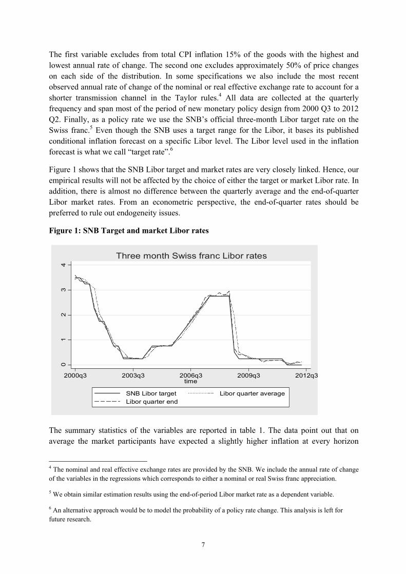
The first variable excludes from total CPI inflation 15% of the goods with the highest and lowest annual rate of change. The second one excludes approximately 50% of price changes on each side of the distribution. In some specifications we also include the most recent observed annual rate of change of the nominal or real effective exchange rate to account for a shorter transmission channel in the Taylor rules.4 All data are collected at the quarterly frequency and span most of the period of new monetary policy design from 2000 Q3 to 2012 Q2. Finally, as a policy rate we use the SNB’s official three-month Libor target rate on the Swiss franc.5 Even though the SNB uses a target range for the Libor, it bases its published conditional inflation forecast on a specific Libor level. The Libor level used in the inflation forecast is what we call “target rate”.6

Figure 1 shows that the SNB Libor target and market rates are very closely linked. Hence, our empirical results will not be affected by the choice of either the target or market Libor rate. In addition, there is almost no difference between the quarterly average and the end-of-quarter Libor market rates. From an econometric perspective, the end-of-quarter rates should be preferred to rule out endogeneity issues.

Figure 1: SNB Target and market Libor rates

01

23

4

2000q3 2003q3 2006q3 2009q3 2012q3time

SNB Libor target Libor quarter average Libor quarter end

Three month Swiss franc Libor rates

The summary statistics of the variables are reported in table 1. The data point out that on average the market participants have expected a slightly higher inflation at every horizon

4 The nominal and real effective exchange rates are provided by the SNB. We include the annual rate of change of the variables in the regressions which corresponds to either a nominal or real Swiss franc appreciation.

5 We obtain similar estimation results using the end-of-period Libor market rate as a dependent variable.

6 An alternative approach would be to model the probability of a policy rate change. This analysis is left for future research.

8

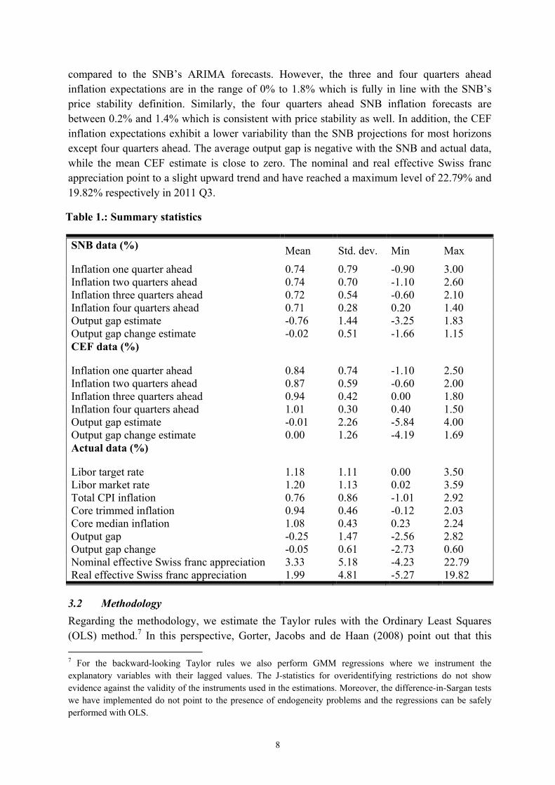
compared to the SNB’s ARIMA forecasts. However, the three and four quarters ahead inflation expectations are in the range of 0% to 1.8% which is fully in line with the SNB’s price stability definition. Similarly, the four quarters ahead SNB inflation forecasts are between 0.2% and 1.4% which is consistent with price stability as well. In addition, the CEF inflation expectations exhibit a lower variability than the SNB projections for most horizons except four quarters ahead. The average output gap is negative with the SNB and actual data, while the mean CEF estimate is close to zero. The nominal and real effective Swiss franc appreciation point to a slight upward trend and have reached a maximum level of 22.79% and 19.82% respectively in 2011 Q3.

Table 1.: Summary statistics

SNB data (%) Mean Std. dev. Min Max

Inflation one quarter ahead 0.74 0.79 -0.90 3.00 Inflation two quarters ahead 0.74 0.70 -1.10 2.60 Inflation three quarters ahead 0.72 0.54 -0.60 2.10 Inflation four quarters ahead 0.71 0.28 0.20 1.40 Output gap estimate -0.76 1.44 -3.25 1.83 Output gap change estimate -0.02 0.51 -1.66 1.15 CEF data (%)

Inflation one quarter ahead 0.84 0.74 -1.10 2.50 Inflation two quarters ahead 0.87 0.59 -0.60 2.00 Inflation three quarters ahead 0.94 0.42 0.00 1.80 Inflation four quarters ahead 1.01 0.30 0.40 1.50 Output gap estimate -0.01 2.26 -5.84 4.00 Output gap change estimate 0.00 1.26 -4.19 1.69 Actual data (%)

Libor target rate 1.18 1.11 0.00 3.50 Libor market rate 1.20 1.13 0.02 3.59 Total CPI inflation 0.76 0.86 -1.01 2.92 Core trimmed inflation 0.94 0.46 -0.12 2.03 Core median inflation 1.08 0.43 0.23 2.24 Output gap -0.25 1.47 -2.56 2.82 Output gap change -0.05 0.61 -2.73 0.60 Nominal effective Swiss franc appreciation 3.33 5.18 -4.23 22.79 Real effective Swiss franc appreciation 1.99 4.81 -5.27 19.82

3.2 Methodology Regarding the methodology, we estimate the Taylor rules with the Ordinary Least Squares (OLS) method.7 In this perspective, Gorter, Jacobs and de Haan (2008) point out that this 7 For the backward-looking Taylor rules we also perform GMM regressions where we instrument the explanatory variables with their lagged values. The J-statistics for overidentifying restrictions do not show evidence against the validity of the instruments used in the estimations. Moreover, the difference-in-Sargan tests we have implemented do not point to the presence of endogeneity problems and the regressions can be safely performed with OLS.

9

approach is justified by the use of forecasts and expectations variables based on real-time data. We have also tested the series for stationarity using the standard Augmented Dickey-Fuller (ADF), Phillips-Perron (PP) and Kwiatkowski–Phillips–Schmidt–Shin (KPSS) tests. The ADF and PP tests show that in most of the series we reject the unit root hypothesis and the KPSS statistics do not report evidence against stationarity for all series used in the regressions. This result is in line with the economic intuition for stationarity as there has been a stable monetary policy regime in place during the last decade in Switzerland.

In order to study the stability of the Taylor rule coefficients we perform rolling and recursive window regressions and conduct conventional tests for structural breaks. In the rolling estimation we use a window size of 30 observations, while in the recursive approach the estimation range is progressively extended as more observations become available over time. In both approaches, the first regression refers to the period before the financial meltdown, from 2000 Q3 to 2007 Q4.

At a more general level, based on Hastie and Tibshirani (1986 and 1990) we investigate the nonlinearity of the Taylor rule specifications with a semi-parametric modeling approach. The latter is a well suited method to detect nonlinearities in the rules within the support of the explanatory variables. This framework is a special case of a family of semi-parametric models known as Generalized Additive Models (GAMs). As pointed out in Wood (2006), a GAM is a generalized linear model in which the linear predictor is a sum of smooth functions of the explanatory variables. In that regard, the approach requires a method to represent the functions and to estimate their degree of smoothness. Hence, the GAMs are represented through penalized regression splines which are estimated with penalized regression methods in two steps. First, the degree of smoothness is computed with a Generalized Cross Validation (GCV) algorithm. The latter balances the need to fit the data with the requirement to avoid model overfitting. Based on Kim and Gu (2004) we apply an additional penalty term in the GCV procedure to further rule out overfitting. In a second step, the smooth functions are then estimated with Penalized Iterative Reweighted Least Squares (PIRLS) as outlined in Wood (2006). More formally, we solve the following penalized least squares optimization problem:

SXyMin '|||| 2 , where controls the smoothness of the splines and S is a matrix

of terms that penalize wiggliness.

In the empirical analysis, we set up univariate and bivariate models in which the policy rate is set as a smooth function of macroeconomic fundamentals. In the former, the explanatory variables enter additively the Taylor rules, while in the bivariate rules the dependent variable is a single function of all covariates. The univariate and bivariate GAMs are estimated in the R software using the mgcv package developed by Wood. A convenient hallmark of the GAM is that it does not require to provide assumptions on the specific functional form of the Taylor rules which offers considerable flexibility. The GAM methodology is preferred to kernel

10

based estimators because the former relies on orthogonal bases and is distributional-free compared to the Nadaraya-Watson type of estimators.8

4. Theoretical framework In a major contribution, Woodford (2003) advocates the view of central banking as a management of private sector expectations. From this standpoint, the monetary authority aims at anchoring agents’ expectations with its targets to achieve better stabilization outcomes. As argued by Holmsen et al. (2008), some variants of the forward-looking Taylor rules are used by Norges Bank and other inflation targeting central banks to communicate their monetary policy intentions. Regarding Swiss monetary policy, Jordan, Peytrignet and Rossi (2010) highlight that the SNB is not an inflation targeting central bank as it has opted for a more flexible policy design. In addition, as a natural benchmark comparison we consider the standard rule proposed by Taylor (1993) along with some augmented and modified versions that contain backward-looking variables. Consider the following interest rate rule:

ttztqtqttytkttTt zyyEEri || **** (1)

where Tti refers to the three-month Libor target rate on the Swiss franc, *r and * denote the

equilibrium real interest rate and the central bank’s inflation objective respectively.9*

t k and *qtqtt yyx correspond to the inflation and output gaps forecasts k and q

quarters ahead correspondingly and tz refers to other economic fundamentals like the

exchange rate for instance. Finally, tE is the expectations operator and t denotes the available information set of either the central bank or the market participants, and the one based on actual data. t stands for an i.i.d error term.

We can further assume that the central bank implements gradual policy rate adjustments to avoid disruptive effects in financial markets originating from large swings in interest rates. In this case the following partial adjustment mechanism takes place:

1 (1 ) Tt t ti i i (2)

where ti is the observed policy rate, Tti corresponds to the policy rate target and is the

interest rate smoothing parameter. At each quarterly policy meeting the Governing Board implements )1( of the desired target interest rate. Combining equations (1) and (2) yields the following Taylor rule specification:

ttztqtqttytktttt zyyEErii ||1 ****1 (3)

8 The splines rely on basis functions while the kernel estimators use a local constant approximation of the distribution.

9 We set %1* which corresponds to past average inflation. Choosing another numerical value would only affect the constant term in the regressions. Please notice that the SNB’s goal of price stability is expressed as a range such that we have to use past average inflation as the reference.

11

As previously highlighted, in the empirical analysis we consider different forecast horizons for inflation ranging from one to four quarters ahead 1, 2,3, 4k , while we consider only

the contemporaneous output gap estimates mainly due to data availability 0q and also to

account for a shorter transmission lag in the economy. This approach is also in line with Cuche-Curti, Hall and Zanetti (2008) who use the one year ahead inflation rate and the contemporaneous output gap in the estimation of their Taylor rule. In the backward-looking Taylor rules we use the actual annual CPI inflation and the output gap obtained with the production function approach. We additionally present the regression results with the SNB core inflation variables to study the central bank’s reaction to these narrower inflation measures.

Based on equations (1) and (3), we analyze 48 forward-looking specifications and 6 backward-looking Taylor rules that are estimated with the SNB, CEF and actual data. In the next section, we report the empirical results from the linear parametric estimations and discuss the stability of the coefficients.

5. Parametric Taylor rules

5.1 Linear model estimations In this subsection we report the estimation results of the best fitting forward and backward-looking Taylor rules. The specifications are presented in the appendix where I stands for inflation, O for output gap, E and Q for nominal and real effective appreciation correspondingly, S for interest rate smoothing, B and F for backward and forward-looking rules respectively. First, in the spirit of a strict inflation targeting approach, IFj contain only the inflation forecasts as explanatory variables ranging from one to four quarters ahead. The goal of these specifications is to study how the policy rate responds to inflation along the forecast horizon. Second, in rules IOFj we additionally include a reaction to the contemporaneous output gap estimate to determine to what extent the SNB takes due account of the economic outlook in setting the Libor target rate. Furthermore, we account for a faster transmission channel in a small open economy through either the nominal or real effective appreciation of the Swiss franc in rules IOEFj and IOQFj and in specifications IEFj and IQFj

respectively without the output gap estimate. In line with the literature, we set up a partial adjustment mechanism in rules IOSFj, IOESFj, IOQSFj, ISFj, IESFj and IQSFj to model the central bank’s practice of interest rate smoothing. This approach should permit to understand how quickly the policy rate is adjusted to the desired target level. Finally, with the aim to shed new light on Taylor’s rule’ original formulation we provide evidence on some backward-looking specifications in the appendix. In the latter, IOB corresponds to the standard Taylor rule while IOEB and IOQB refer to the augmented models with either a nominal or real effective appreciation of the Swiss franc. IOSB, IOESB and IOQSB relate to the corresponding backward-looking Taylor rules with interest rate smoothing.

5.1.1 Taylor rules with focus only on inflation forecast We first start the empirical analysis by presenting the estimation results of the forward-looking Taylor rules that account only for a central bank’s responsiveness to the inflation

12

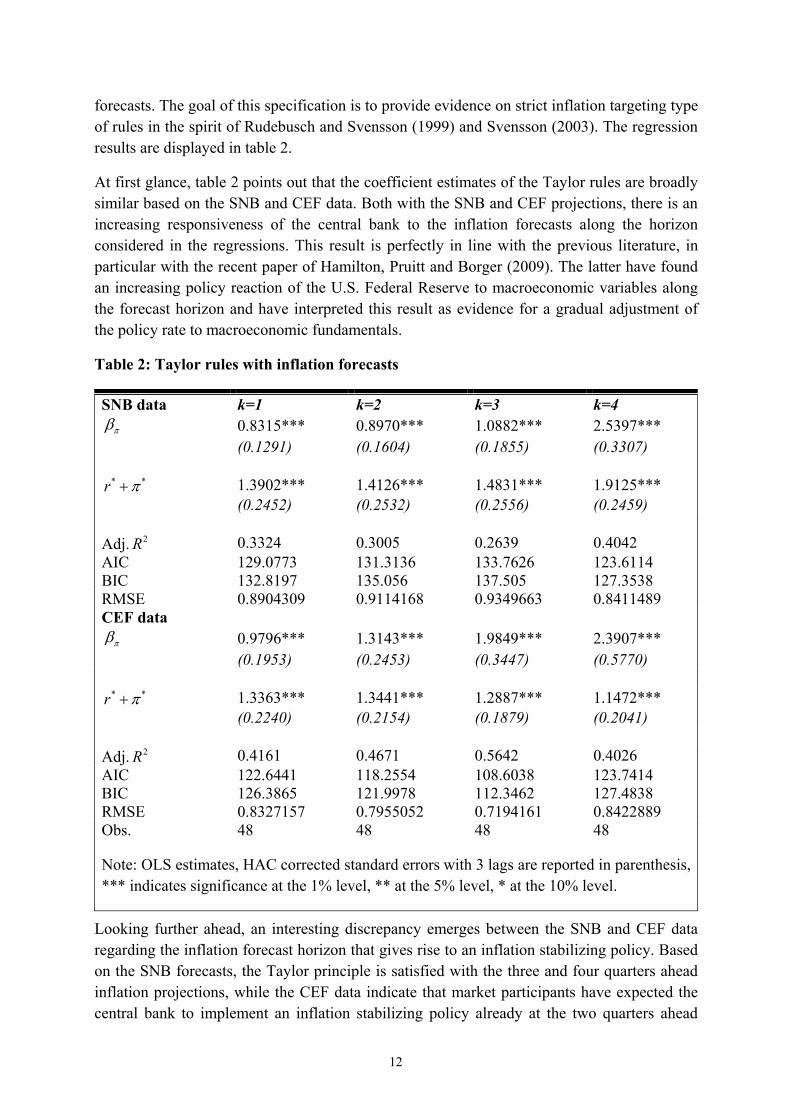
forecasts. The goal of this specification is to provide evidence on strict inflation targeting type of rules in the spirit of Rudebusch and Svensson (1999) and Svensson (2003). The regression results are displayed in table 2.

At first glance, table 2 points out that the coefficient estimates of the Taylor rules are broadly similar based on the SNB and CEF data. Both with the SNB and CEF projections, there is an increasing responsiveness of the central bank to the inflation forecasts along the horizon considered in the regressions. This result is perfectly in line with the previous literature, in particular with the recent paper of Hamilton, Pruitt and Borger (2009). The latter have found an increasing policy reaction of the U.S. Federal Reserve to macroeconomic variables along the forecast horizon and have interpreted this result as evidence for a gradual adjustment of the policy rate to macroeconomic fundamentals.

Table 2: Taylor rules with inflation forecasts

SNB data k=1 k=2 k=3 k=4 0.8315*** 0.8970*** 1.0882*** 2.5397*** (0.1291) (0.1604) (0.1855) (0.3307)

* *r 1.3902*** 1.4126*** 1.4831*** 1.9125*** (0.2452) (0.2532) (0.2556) (0.2459)

Adj. 2R 0.3324 0.3005 0.2639 0.4042 AICBIC

129.0773132.8197

131.3136135.056

133.7626137.505

123.6114127.3538

RMSE 0.8904309 0.9114168 0.9349663 0.8411489 CEF data

0.9796*** 1.3143*** 1.9849*** 2.3907*** (0.1953) (0.2453) (0.3447) (0.5770)

* *r 1.3363*** 1.3441*** 1.2887*** 1.1472*** (0.2240) (0.2154) (0.1879) (0.2041)

Adj. 2R 0.4161 0.4671 0.5642 0.4026 AICBIC

122.6441126.3865

118.2554121.9978

108.6038112.3462

123.7414127.4838

RMSE 0.8327157 0.7955052 0.7194161 0.8422889 Obs. 48 48 48 48

Note: OLS estimates, HAC corrected standard errors with 3 lags are reported in parenthesis, *** indicates significance at the 1% level, ** at the 5% level, * at the 10% level.

Looking further ahead, an interesting discrepancy emerges between the SNB and CEF data regarding the inflation forecast horizon that gives rise to an inflation stabilizing policy. Based on the SNB forecasts, the Taylor principle is satisfied with the three and four quarters ahead inflation projections, while the CEF data indicate that market participants have expected the central bank to implement an inflation stabilizing policy already at the two quarters ahead

13

horizon. Overall, there is a stronger reaction to the inflation forecasts based on the CEF data except at the four quarters ahead horizon.

From an information criterion perspective, the AIC and BIC statistics suggest that the best model is the one with the four and three quarters ahead inflation forecasts respectively with the SNB and CEF data. The RMSE statistics corroborate the evidence from the information criteria for the best fitting model.

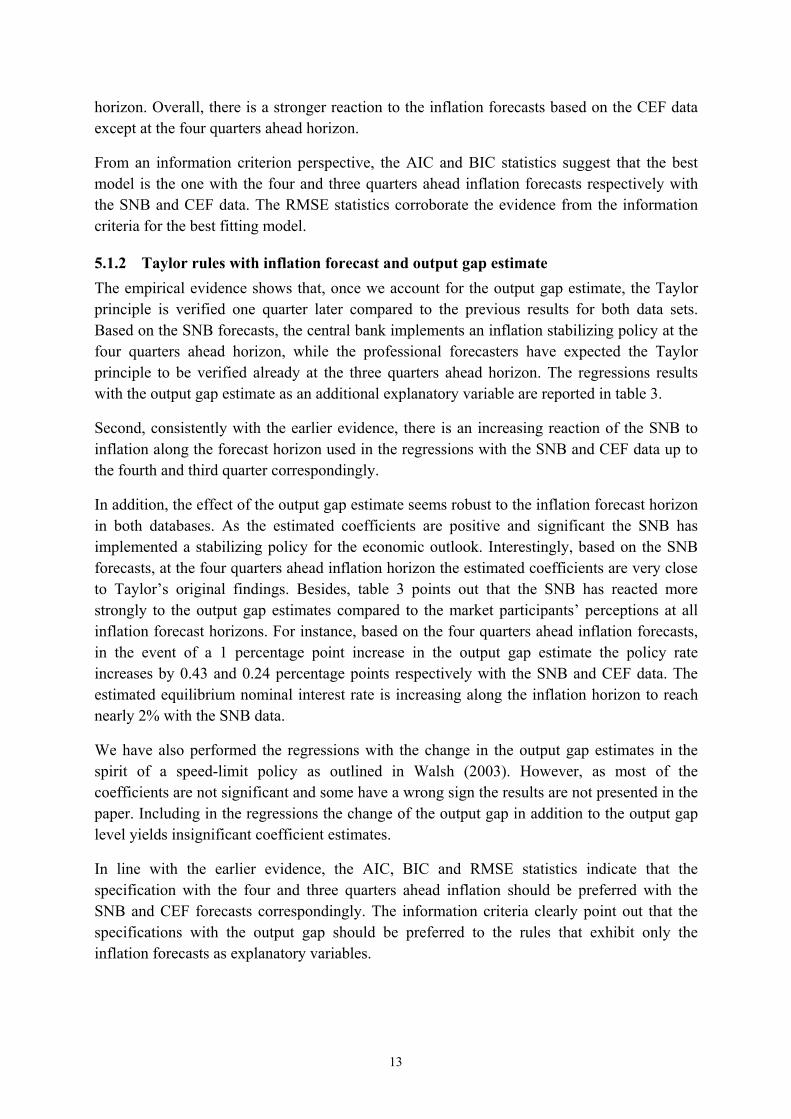
5.1.2 Taylor rules with inflation forecast and output gap estimate The empirical evidence shows that, once we account for the output gap estimate, the Taylor principle is verified one quarter later compared to the previous results for both data sets. Based on the SNB forecasts, the central bank implements an inflation stabilizing policy at the four quarters ahead horizon, while the professional forecasters have expected the Taylor principle to be verified already at the three quarters ahead horizon. The regressions results with the output gap estimate as an additional explanatory variable are reported in table 3.

Second, consistently with the earlier evidence, there is an increasing reaction of the SNB to inflation along the forecast horizon used in the regressions with the SNB and CEF data up to the fourth and third quarter correspondingly.

In addition, the effect of the output gap estimate seems robust to the inflation forecast horizon in both databases. As the estimated coefficients are positive and significant the SNB has implemented a stabilizing policy for the economic outlook. Interestingly, based on the SNB forecasts, at the four quarters ahead inflation horizon the estimated coefficients are very close to Taylor’s original findings. Besides, table 3 points out that the SNB has reacted more strongly to the output gap estimates compared to the market participants’ perceptions at all inflation forecast horizons. For instance, based on the four quarters ahead inflation forecasts, in the event of a 1 percentage point increase in the output gap estimate the policy rate increases by 0.43 and 0.24 percentage points respectively with the SNB and CEF data. The estimated equilibrium nominal interest rate is increasing along the inflation horizon to reach nearly 2% with the SNB data.

We have also performed the regressions with the change in the output gap estimates in the spirit of a speed-limit policy as outlined in Walsh (2003). However, as most of the coefficients are not significant and some have a wrong sign the results are not presented in the paper. Including in the regressions the change of the output gap in addition to the output gap level yields insignificant coefficient estimates.

In line with the earlier evidence, the AIC, BIC and RMSE statistics indicate that the specification with the four and three quarters ahead inflation should be preferred with the SNB and CEF forecasts correspondingly. The information criteria clearly point out that the specifications with the output gap should be preferred to the rules that exhibit only the inflation forecasts as explanatory variables.

14

Table 3: Taylor rules with inflation forecasts and output gap estimates

SNB data k=1, q=0 k=2, q=0 k=3, q=0 k=4, q=0 0.5012*** 0.5599*** 0.7006*** 1.6277*** (0.1287) (0.1179) (0.1397) (0.3279)

y 0.4557*** 0.4706*** 0.4857*** 0.4315*** (0.0688) (0.0663) (0.0648) (0.0490)

* *r 1.6520*** 1.6818*** 1.7434*** 1.9765*** (0.2062) (0.2011) (0.1931) (0.1909)

Adj. 2R 0.6218 0.6239 0.6211 0.6589 AICBIC

102.7491108.3627

102.4812108.0948

102.8271108.4407

97.78964103.4032

RMSE 0.662897 0.6610498 0.6634361 0.6295208 CEF data

0.5285** 0.8152*** 1.3849*** 1.2507** (0.2256) (0.2194) (0.3388) (0.5697)

y 0.2362*** 0.2229*** 0.1955*** 0.2414*** (0.0826) (0.0682) (0.0574) (0.0688)

* *r 1.2642*** 1.2818*** 1.2560*** 1.1627*** (0.1700) (0.1694) (0.1617) (0.1781)

Adj. 2R 0.5487 0.5974 0.6646 0.5419 AICBIC

111.2301116.8437

105.7477111.3613

96.97598102.5896

111.9405117.5541

RMSE 0.7241248 0.6839299 0.6242077 0.7295029 Obs. 48 48 48 48


To sum up, the evidence shows that in the short run, one to two quarters ahead, the SNB stabilizes primarily business cycle fluctuations as it can hardly affect inflation within a short time span. Conversely, at a longer horizon, three or four quarters ahead, the monetary authority focuses on stabilizing inflation in line with its price stability mandate.

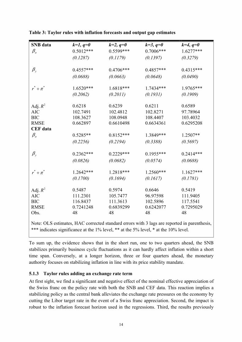
5.1.3 Taylor rules adding an exchange rate term At first sight, we find a significant and negative effect of the nominal effective appreciation of the Swiss franc on the policy rate with both the SNB and CEF data. This reaction implies a stabilizing policy as the central bank alleviates the exchange rate pressures on the economy by cutting the Libor target rate in the event of a Swiss franc appreciation. Second, the impact is robust to the inflation forecast horizon used in the regressions. Third, the results previously

15

obtained with the inflation forecasts and the output gap estimates remain qualitatively unaltered from including the exchange rate in the Taylor rules.10

Table 4: Taylor rules augmented with a nominal effective appreciation


y 0.4607*** 0.4776*** 0.4920*** 0.4366*** (0.0562) (0.0592) (0.0608) (0.0482)

e -0.0522*** -0.0485** -0.0470** -0.0502*** (0.0181) (0.0188) (0.0195) (0.0164)

* *r 1.8085*** 1.8191*** 1.8603*** 2.0858*** (0.2180) (0.2156) (0.2097) (0.1993)

Adj. 2R 0.6728 0.6648 0.6576 0.7066 AICBIC

96.71204104.1968

97.87471105.3595

98.88814106.3729

91.4790998.96389

RMSE 0.6096594 0.617088 0.6236368 0.5773165 CEF data

0.4107** 0.6640*** 1.2041*** 1.4129*** (0.1754) (0.2010) (0.3514) (0.4727)

y 0.2602*** 0.2453*** 0.2148*** 0.2275*** (0.0655) (0.0620) (0.0573) (0.0686)

e -0.0661*** -0.0614*** -0.0586*** -0.0810*** (0.0207) (0.0217) (0.0209) (0.0222)

* *r 1.4654*** 1.4671*** 1.4409*** 1.4304*** (0.1792) (0.1692) (0.1411) (0.1555)

Adj. 2R 0.6355 0.6708 0.7329 0.6821 AICBIC

101.8906109.3754

96.99865104.4835

86.9707894.45558

95.32946102.8143

RMSE 0.6434496 0.6114823 0.5508316 0.6009421 Obs. 48 48 48 48


10 It is also worth mentioning that the correlations between the explanatory variables are quite low which suggests that there are no collinearity problems in the regressions.

16

Table 4 displays the coefficient estimates of the forward-looking Taylor rules augmented with a nominal effective Swiss franc appreciation.11 Based on the SNB forecasts, the central bank implements an inflation stabilizing policy at the four quarters ahead horizon, while the market participants have expected the Taylor principle to be fulfilled already at the three quarters ahead horizon. Besides, the SNB’s reaction to the output gap estimates is in line with the earlier evidence with both the SNB and CEF data. The empirical results are similar with the CEF data, notwithstanding a smaller output gap coefficient estimate and a slightly higher central bank’s reaction to the exchange rate. Thus, following a 1 percentage point nominal effective appreciation the monetary authority decreases the Libor target rate by 0.05 and 0.08 percentage points respectively based on the SNB and CEF data. From a model selection perspective, the AIC, BIC and the RMSE statistics show that the best specification features four and three quarters ahead inflation forecasts with the SNB and CEF data respectively.

In general, table 4 suggests that the SNB has reacted relatively less strongly to the inflation forecasts than to the output gap estimates based on the internal data compared to the market participants’ perceptions.12 Moreover, the empirical fit of the Taylor rules is further enhanced by including an exchange rate term in the regressions as evidenced by the reported relevant statistics.

5.1.4 Summary of results for Taylor rules with partial adjustment Overall, the results for estimations of Taylor rules with a partial adjustment mechanism point to a substantial degree of interest rate smoothing which is slightly more pronounced with the CEF data than with the SNB forecasts. In general, the policy rate is adjusted to the desired target level within a period ranging from three to five quarters. To conserve space, we report the details in tables A.1. and A.2. in the appendix. The main results can be summarized as follows.

As previously found, table A.1. shows that there is an increasing reaction of the central bank to inflation along the forecast horizon up to four and three quarters ahead respectively with the SNB and CEF data. However, compared to the results of table 3 the SNB implements an inflation stabilizing policy already at the two and three quarters ahead horizons correspondingly based on the CEF and SNB estimates, which is one quarter in-advance than previously found. With the CEF database, all output gap and some inflation forecast coefficient estimates are not statistically significant which might cast doubts on the empirical validity of the Taylor rule specification with interest rate smoothing. Indeed, in two seminal papers Rudebusch (2002 and 2006) argues that the estimation of interest rate rules with policy inertia at the quarterly frequency is prone to substantial caveats. He shows that the resulting high predictive ability of the estimated Taylor rules with interest rate smoothing is inconsistent with the evidence from the term structure of interest rates. Besides, relying on a 11 We do not present the estimation results with the real effective appreciation of the Swiss franc as they are qualitatively very similar.

12 The evidence for a relatively stronger central bank’s reaction to the output gap estimates than to the inflation forecasts obtained with the SNB data might be related to an important informational content of the output gap estimates about future inflation in addition to the ARIMA forecasts.

17

new database of models, Taylor and Wieland (2009) show that rules that contain policy inertia in addition to the growth rate of output are not robust. The large autoregressive coefficient of the interest rate, which is often found empirically, may point to a possible model misspecification and is likely to capture persistent shocks rather than to correspond with the central bank’s practice of smoothing the policy rate. Table A.1. reports that the SNB’s reaction to the output gap estimate is slightly dampened once we account for interest rate smoothing in the estimated rules with the SNB and CEF data. In line with the earlier evidence, market participants have expected a relatively stronger central bank’s reaction to the inflation forecasts than to the output gap estimates. From a model selection perspective, the AIC, BIC and RMSE statistics suggest that the specification with the three quarters ahead inflation forecasts should be preferred with both databases.

Table A.2. points to a more strongly negative and significant effect of the nominal effective Swiss franc appreciation on the policy rate than previously obtained in the Taylor rules without smoothing. The policy inertia and inflation coefficients are slightly reduced while the output gap estimates are robust to including the exchange rate in the regressions. Moreover, with both the SNB and CEF data the Taylor principle is verified already at the three quarters ahead inflation forecast horizon. In addition, most of the output gap and some inflation forecast estimates are not significant with the CEF data as previously reported. Broadly, accounting for a partial adjustment mechanism in the augmented forward-looking Taylor rules entails a twice as strong central bank’s reaction to the nominal appreciation of the domestic currency than found without interest rate smoothing. Finally, the AIC, BIC and RMSE criteria point to the model with three quarters ahead inflation forecasts as the best specification, consistently with the results from table A.1.

Furthermore, we have also estimated the Taylor rules augmented with the forecasts of the nominal and real appreciation of the Swiss franc ranging from one to four quarters ahead. As a data generating process, we have assumed a random walk for the level of the nominal and real effective exchange rate. However, the empirical evidence is not satisfactory as it points to a weak and positive relation between the nominal or real effective appreciation and the Libor target rate in all rules, and thus the results are not reported. Besides, the other forward-looking specifications from the appendix perform worse in describing the central bank’s interest rate setting and the estimation results are available on demand.

Finally, we discuss the estimation results of the backward-looking Taylor rules with three different measures of inflation: total CPI, core trimmed and core median inflation respectively.

5.1.5 Summary of results for backward-looking Taylor rules At first sight, the empirical evidence is quite surprising as it raises concerns about the relevance of actual CPI inflation in the backward-looking Taylor rules. Indeed, the estimated inflation coefficients are mostly not significant and the Taylor principle is not satisfied in neither specification. The results also provide a weak evidence on the monetary authority’s responsiveness to the core inflation measures. In light of the findings, the central bank’s behavior seems to substantially differ with the forward or backward-looking data used in the

18

estimation of the Taylor rules which is consistent with the results in the literature. Again, to conserve space, the detailed results are reported in tables A.3. to A.6. in the appendix.

In addition, we report a strong and robust effect of the output gap on the policy rate whose magnitude is similar to the output gap coefficient estimates obtained with the forward-looking Taylor rules. The estimation results are also qualitatively unaltered from including the nominal effective Swiss franc appreciation in the regressions as shown in table A.4. The effect of the nominal effective appreciation is of a similar size than obtained in the forward-looking specifications.13 The Taylor rules with partial adjustment do not yield satisfactory results as in most cases the inflation coefficient is not significant and is further negative in some specifications. The exchange rate estimates point to a robust negative and stronger response to the Swiss franc nominal effective appreciation.

In a nutshell, the empirical evidence suggests that we should rely on forward-looking specifications of the SNB Taylor rules rather than on backward-looking rules. Additionally reacting to the nominal effective Swiss franc appreciation permits to track more closely the Libor target rate set by the SNB Governing Board and suggests a stabilizing effect on the business cycle. In view of the model selection statistics, the best fitting model without interest rate smoothing involves the four quarters ahead inflation forecasts based on the SNB data. With interest smoothing the best fitting Taylor rules contain the three quarters ahead inflation forecasts. As regards the CEF data, the best fitting models are obtained with the inflation forecasts three quarters ahead regardless of the presence of a partial adjustment mechanism. In terms of the RMSE criterion the best specification without interest rate smoothing is IOEFj

with an inflation horizon of four and three quarters ahead respectively for the SNB and CEF data.

5.2 Stability of the Taylor rules and structural break tests In this subsection we first perform rolling and recursive window regressions of the baseline forward and backward-looking rules presented in the paper. The aim is to investigate the stability of the Taylor rules parameters over time particularly during the recent financial crisis. In the rolling approach we apply a fixed window of 30 observations in the estimations, while in the recursive regressions the window size is progressively extended by one quarter over time. In both procedures the first estimation spans the period before the financial turmoil from 2000 Q3 to 2007 Q4.14 In a second step, we perform structural break tests.

5.2.1 Stability of Taylor rules In general, the rolling and recursive regressions do not show evidence for important time variation in the Taylor rules parameters based on the SNB, CEF and actual data. In particular, 13 The regressions with the real effective appreciation of the Swiss franc are not reported as they yield very similar results. In addition, the regressions with the change in the output gap are not presented neither as the coefficient estimates are mostly not significant.

14 We have choosen a window size of 30 observations in order to obtain statistically reliable results. To save some space the estimated coefficients are not presented in the paper but are available from the authors on demand.

19

there is no evidence that the SNB’s responsiveness to economic fundamentals has fundamentally changed neither at the peak of the financial crisis nor since the introduction of the Swiss franc floor against the euro. Besides, the coefficient estimates from the rolling and recursive regressions are qualitatively similar.15

The forward-looking Taylor rules with only the inflation forecast gap as explanatory variable feature quite stable coefficients over time. Including a reaction to the output gap estimate in the rules leads to a higher variation in the coefficients even though it does not suggest the presence of a break. The Taylor rules that account for an exchange rate responsiveness point out that the estimated coefficient has gradually decreased and has turned negative since late 2009, thus implying a stabilizing central bank’s policy on the economy. The rules with policy inertia show that there has been a temporary and gradual decrease in interest rate smoothing at the peak of the financial downturn, while thereafter the estimated coefficient has returned to its pre-crisis level. Finally, the augmented forward-looking Taylor rules with policy inertia and exchange rate responsiveness indicate that, although there is some time variation in the interest rate smoothing, inflation forecast gap and output gap coefficients, the exchange rate estimate has remained broadly stable. Importantly, the magnitude of the exchange rate reaction is in line with the evidence from the linear estimations.

A comparison of the empirical results obtained with the SNB and CEF data reveals that they are qualitatively similar for many specifications. However, the findings suggest that the market participants have expected an increasing inflation reaction of the central bank relative to the economic outlook over time compared to the estimates obtained with the SNB data. This result might point out that as inflationary pressures have dampened in the midst of the crisis, the central bank has put a relatively higher emphasis on business cycle considerations and on securing the stability of the financial system.

The backward-looking Taylor rules do not exhibit a high variation in the coefficients, although they point to some gradual change in the inflation and output gaps responsiveness. Consistently with the previous results, the exchange rate coefficient turns negative from 2010 on thus implying a stabilizing central bank’s policy for the economy. The specification with policy inertia shows that the interest rate smoothing has temporarily decreased at the tipping point of the crisis as previously found. Finally, there is no evidence that the Taylor principle has been fulfilled based on actual data which is in line with the findings from the linear regressions.

5.2.2 Tests of structural breaks Most of the test statistics seem to support the presence of a structural break in the Taylor rules occurring at the peak of the financial crisis in 2008 Q3. However, we have to highlight that the relevant tests are performed with a relatively small number of observations, which might undermine the accuracy of the test statistics. Additionally, Kahn (2012) brings to the fore that it is still an open question whether Taylor rules have undergone a fundamental structural

15 To conserve space, the graphs of the rolling and recursive windows are not reported but are available on demand.

20

change during the financial crisis. In view of the previous arguments the results from the tests should be interpreted with particular caution.

Based on Hansen (2001), we have performed several tests for a break in the Taylor rules coefficients following the recent advances in the design of time series tests for structural change. First, relying on the approach of Chow (1960) we have implemented tests for a break occurring either at the onset of the crisis in 2007 Q3 or at the peak of the downturn in 2008 Q3. For the former, the F statistics do not show evidence for a break in the coefficients of the Taylor rules. However, for the latter the Chow statistics suggest that there has been a change in the parameters after the Lehman Brothers collapse in most rules. Second, we have applied Andrews (1993) tests of structural change with an unknown break date with a trimming of 25%. The results corroborate the evidence for a break in the coefficients occurring in 2008 Q3. Finally, we have performed the Bai and Perron (1998 and 2003) sequential procedure to estimate the number of breaks and test for multiple structural changes based on the Sup FT(l+1|l) statistic. Given the relatively small number of observations and the applied high trimming the tests allow for a maximum of two breaks. The results tend to confirm the previous evidence for a break in 2008 Q3 and point to a change in some Taylor rules between 2003 Q2 and 2005 Q2 depending on the data and specifications. The latter period refers to the previous cycle of policy accommodation. Nevertheless, when we allow for possible serial correlation and heteroskedasticity in the error structure, the confidence intervals of the break dates are in some cases implausibly large and for some specifications the algorithm does not converge well.

In the rolling and recursive window procedures we assume that the model remains linear over specific periods whereas the Taylor rules parameters can change over time. In addition, in a more general setting, we allow for a nonlinear model in which the reaction of the central bank to economic fundamentals might change along with the level of the explanatory variables. Hence, the semi-parametric approach further complements the stability analysis of the Taylor rules by investigating the relationship between the policy rate and the covariates.

6. Semi-parametric Taylor rules In this section we present the regression results of the Taylor rules estimated with a semi-parametric approach. In order to investigate the nonlinearity of the Taylor rules within the support of the explanatory variables we estimate two types of specifications: univariate and bivariate rules. In the former, the policy rate is a sum of additive smooth functions of the explanatory variables whereas in the latter the dependent variable is a single spline of all covariates. From a statistical perspective, the univariate rules exhibit a faster rate of convergence whereas the bivariate rules are exposed to a possible curse of dimensionality problem. 16 Nonetheless, the bivariate regression is more general as it allows for a possible interaction between the explanatory variables and provides a convenient visual approach to describe the Taylor rules. With the semi-parametric technique, the nonlinearity is defined as a

16 The latter corresponds to a slower rate of asymptotic convergence of the spline along with the dimension considered. The bivariate specification has a rate of convergence of n-2/3 compared to the rate of n-4/5 and n-1 in the univariate and parametric rules respectively.

21

changing central bank’s responsiveness to economic fundamentals along the level of the explanatory variables and is reflected in the shape of the estimated splines.

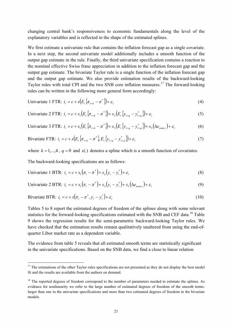
We first estimate a univariate rule that contains the inflation forecast gap as a single covariate. In a next step, the second univariate model additionally includes a smooth function of the output gap estimate in the rule. Finally, the third univariate specification contains a reaction to the nominal effective Swiss franc appreciation in addition to the inflation forecast gap and the output gap estimate. The bivariate Taylor rule is a single function of the inflation forecast gap and the output gap estimate. We also provide estimation results of the backward-looking Taylor rules with total CPI and the two SNB core inflation measures.17 The forward-looking rules can be written in the following more general form accordingly:

Univariate 1 FTR: tkttt Esci * (4)

Univariate 2 FTR: tqtqttkttt yyEsEsci *2

*1 (5)

Univariate 3 FTR: ttnomqtqttkttt esyyEsEsci ,3*

2*

1 (6)

Bivariate FTR: tqtqttkttt yyEEsci ** , (7)

where 4,...,1k , 0q and (.)s denotes a spline which is a smooth function of covariates.

The backward-looking specifications are as follows:

Univariate 1 BTR: ttttt yyssci *2

*1 (8)

Univariate 2 BTR: ttnomtttt esyyssci ,3*

2*

1 (9)

Bivariate BTR: ttttt yysci ** , (10)

Tables 5 to 8 report the estimated degrees of freedom of the splines along with some relevant statistics for the forward-looking specifications estimated with the SNB and CEF data.18 Table 9 shows the regression results for the semi-parametric backward-looking Taylor rules. We have checked that the estimation results remain qualitatively unaltered from using the end-of-quarter Libor market rate as a dependent variable.

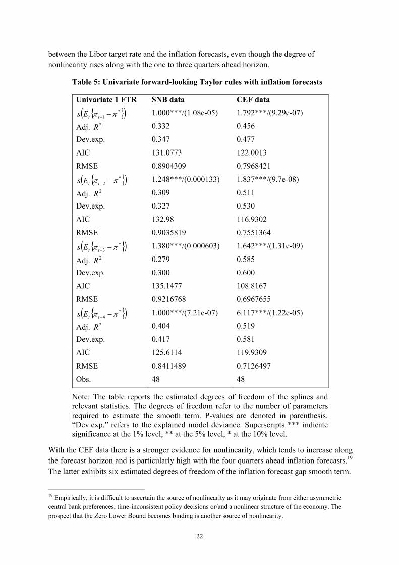
The evidence from table 5 reveals that all estimated smooth terms are statistically significant in the univariate specifications. Based on the SNB data, we find a close to linear relation

17 The estimations of the other Taylor rules specifications are not presented as they do not display the best model fit and the results are available from the authors on demand.

18 The reported degrees of freedom correspond to the number of parameters needed to estimate the splines. As evidence for nonlinearity we refer to the large number of estimated degrees of freedom of the smooth terms: larger than one in the univariate specifications and more than two estimated degrees of freedom in the bivariate models.

22

between the Libor target rate and the inflation forecasts, even though the degree of nonlinearity rises along with the one to three quarters ahead horizon.

Table 5: Univariate forward-looking Taylor rules with inflation forecasts

Univariate 1 FTR SNB data CEF data *

1ttEs 1.000***/(1.08e-05) 1.792***/(9.29e-07)

Adj. 2R 0.332 0.456

Dev.exp. 0.347 0.477

AIC 131.0773 122.0013

RMSE 0.8904309 0.7968421 *

2ttEs 1.248***/(0.000133) 1.837***/(9.7e-08)

Adj. 2R 0.309 0.511

Dev.exp. 0.327 0.530

AIC 132.98 116.9302

RMSE 0.9035819 0.7551364 *

3ttEs 1.380***/(0.000603) 1.642***/(1.31e-09)

Adj. 2R 0.279 0.585

Dev.exp. 0.300 0.600

AIC 135.1477 108.8167

RMSE 0.9216768 0.6967655 *

4ttEs 1.000***/(7.21e-07) 6.117***/(1.22e-05)

Adj. 2R 0.404 0.519

Dev.exp. 0.417 0.581

AIC 125.6114 119.9309

RMSE 0.8411489 0.7126497

Obs. 48 48

Note: The table reports the estimated degrees of freedom of the splines and relevant statistics. The degrees of freedom refer to the number of parameters required to estimate the smooth term. P-values are denoted in parenthesis. “Dev.exp.” refers to the explained model deviance. Superscripts *** indicate significance at the 1% level, ** at the 5% level, * at the 10% level.

With the CEF data there is a stronger evidence for nonlinearity, which tends to increase along the forecast horizon and is particularly high with the four quarters ahead inflation forecasts.19

The latter exhibits six estimated degrees of freedom of the inflation forecast gap smooth term.

19 Empirically, it is difficult to ascertain the source of nonlinearity as it may originate from either asymmetric central bank preferences, time-inconsistent policy decisions or/and a nonlinear structure of the economy. The prospect that the Zero Lower Bound becomes binding is another source of nonlinearity.

23

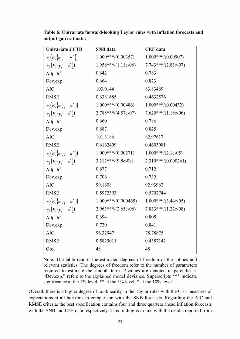
Table 6: Univariate forward-looking Taylor rules with inflation forecasts and output gap estimates


11 ttEs 1.000***/(0.00357) 1.000***/(0.00907) *

2 ttt yyEs 1.958***/(1.11e-06) 7.743***/(2.83e-07)

Adj. 2R 0.642 0.783

Dev.exp. 0.664 0.823

AIC 103.0144 83.83469

RMSE 0.6381685 0.4632576 *

21 ttEs 1.000***/(0.00486) 1.000***/(0.00432) *

2 ttt yyEs 2.788***/(4.57e-07) 7.620***/(1.18e-06)

Adj. 2R 0.660 0.786

Dev.exp. 0.687 0.825

AIC 101.3186 82.97617

RMSE 0.6162409 0.4603081 *

31 ttEs 1.000***/(0.00271) 1.000***/(2.1e-05) *

2 ttt yyEs 3.212***/(9.8e-08) 2.319***/(0.000261)

Adj. 2R 0.677 0.712

Dev.exp. 0.706 0.732

AIC 99.1608 92.93962

RMSE 0.5972393 0.5702744 *

41 ttEs 1.000***/(0.000465) 1.000***/(3.44e-05) *

2 ttt yyEs 2.963***/(2.65e-06) 7.833***/(1.22e-08)

Adj. 2R 0.694 0.805

Dev.exp. 0.720 0.841

AIC 96.32947 78.78875

RMSE 0.5829011 0.4387142

Obs. 48 48


Overall, there is a higher degree of nonlinearity in the Taylor rules with the CEF measures of expectations at all horizons in comparison with the SNB forecasts. Regarding the AIC and RMSE criteria, the best specification contains four and three quarters ahead inflation forecasts with the SNB and CEF data respectively. This finding is in line with the results reported from

24

the parametric regressions. Importantly, as there is evidence for nonlinearity in the estimated rules particularly with the CEF data, we obtain a better model fit with the semi-parametric approach than with the parametric Taylor rules.

Table 6 displays the regression results of the univariate Taylor rules where the policy rate is an additive function of the inflation forecast gap and output gap estimate. All estimated smooth functions are significant and the semi-parametric rules feature a higher explanatory power compared to their parametric counterparts.

At first sight, the table suggests that the roots of nonlinearity lie in the output gap estimate smooth term. Indeed, the inflation forecast gap function is linear in all specifications, while the output gap estimate spline is highly nonlinear. The nonlinearity of the output gap could be explained by a more cautious reaction of the SNB to the output gap which is a variable measured with more noise than inflation. In general, the RMSE is smaller compared to the one of the corresponding bivariate Taylor rules from table 8 for most specifications which points to a better model fit achieved with the univariate approach. The rules with the four quarters ahead inflation forecasts feature the best fit with the Libor target rate and are preferred from an information criterion approach.

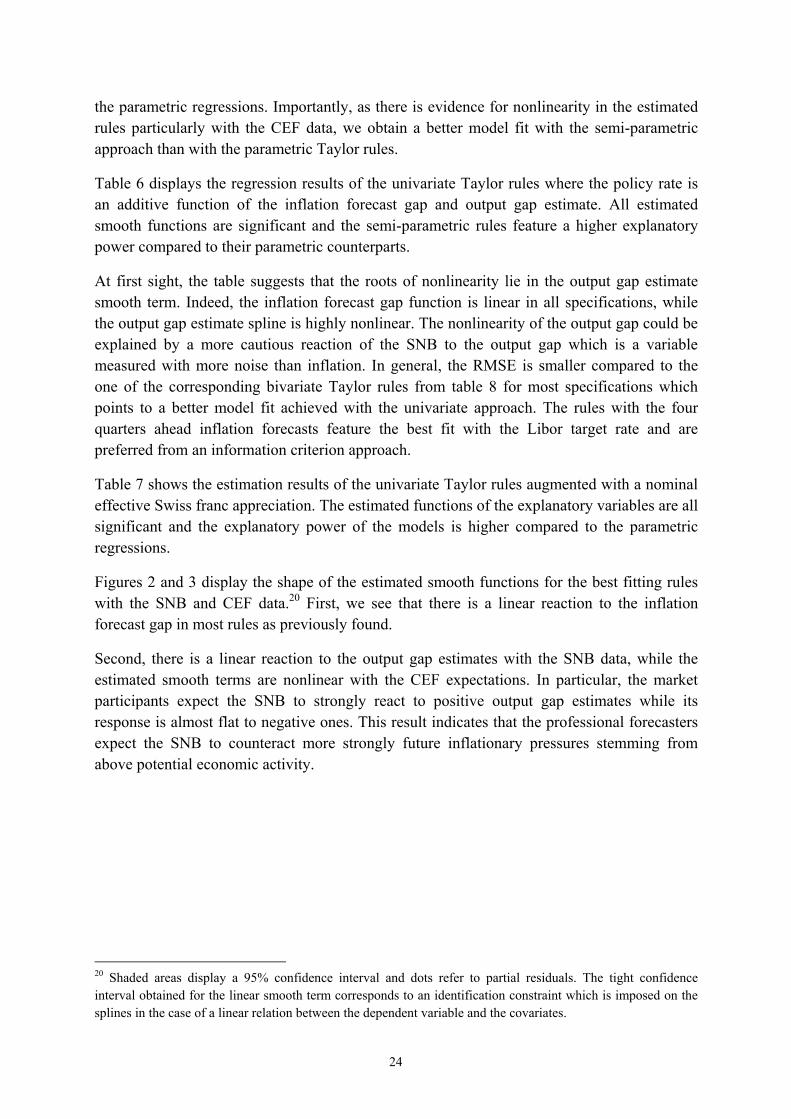
Table 7 shows the estimation results of the univariate Taylor rules augmented with a nominal effective Swiss franc appreciation. The estimated functions of the explanatory variables are all significant and the explanatory power of the models is higher compared to the parametric regressions.

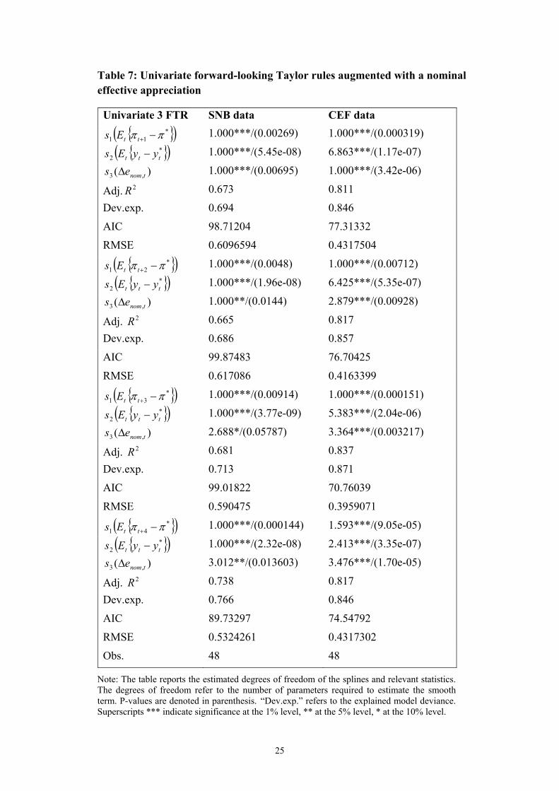
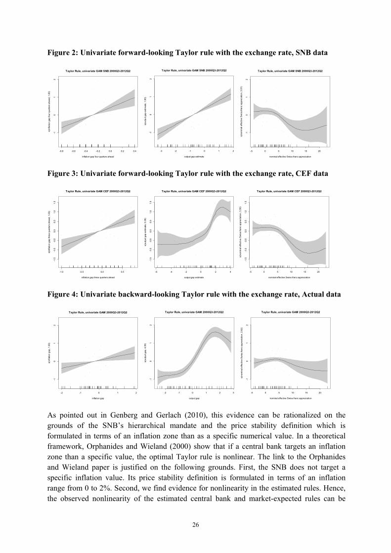
Figures 2 and 3 display the shape of the estimated smooth functions for the best fitting rules with the SNB and CEF data.20 First, we see that there is a linear reaction to the inflation forecast gap in most rules as previously found.

Second, there is a linear reaction to the output gap estimates with the SNB data, while the estimated smooth terms are nonlinear with the CEF expectations. In particular, the market participants expect the SNB to strongly react to positive output gap estimates while its response is almost flat to negative ones. This result indicates that the professional forecasters expect the SNB to counteract more strongly future inflationary pressures stemming from above potential economic activity.

20 Shaded areas display a 95% confidence interval and dots refer to partial residuals. The tight confidence interval obtained for the linear smooth term corresponds to an identification constraint which is imposed on the splines in the case of a linear relation between the dependent variable and the covariates.

25

Table 7: Univariate forward-looking Taylor rules augmented with a nominal effective appreciation


11 ttEs 1.000***/(0.00269) 1.000***/(0.000319) *

2 ttt yyEs 1.000***/(5.45e-08) 6.863***/(1.17e-07)

)( ,3 tnomes 1.000***/(0.00695) 1.000***/(3.42e-06)

Adj. 2R 0.673 0.811

Dev.exp. 0.694 0.846

AIC 98.71204 77.31332

RMSE 0.6096594 0.4317504 *

21 ttEs 1.000***/(0.0048) 1.000***/(0.00712) *

2 ttt yyEs 1.000***/(1.96e-08) 6.425***/(5.35e-07)

)( ,3 tnomes 1.000**/(0.0144) 2.879***/(0.00928)

Adj. 2R 0.665 0.817

Dev.exp. 0.686 0.857

AIC 99.87483 76.70425

RMSE 0.617086 0.4163399 *

31 ttEs 1.000***/(0.00914) 1.000***/(0.000151) *

2 ttt yyEs 1.000***/(3.77e-09) 5.383***/(2.04e-06)

)( ,3 tnomes 2.688*/(0.05787) 3.364***/(0.003217)

Adj. 2R 0.681 0.837

Dev.exp. 0.713 0.871

AIC 99.01822 70.76039

RMSE 0.590475 0.3959071 *

41 ttEs 1.000***/(0.000144) 1.593***/(9.05e-05) *

2 ttt yyEs 1.000***/(2.32e-08) 2.413***/(3.35e-07)

)( ,3 tnomes 3.012**/(0.013603) 3.476***/(1.70e-05)

Adj. 2R 0.738 0.817

Dev.exp. 0.766 0.846

AIC 89.73297 74.54792

RMSE 0.5324261 0.4317302

Obs. 48 48


26

Figure 2: Univariate forward-looking Taylor rule with the exchange rate, SNB data

-0.8 -0.6 -0.4 -0.2 0.0 0.2 0.4

-10

12

inflation gap four quarters ahead

s(in

flatio

n ga

p fo

ur q

uarte

rs a

head

, 1.0

0)

Taylor Rule, univariate GAM SNB 2000Q3-2012Q2

-3 -2 -1 0 1 2-1

01

2

output gap estimate

s(ou

tput

gap

est

imat

e, 1

.00)


-5 0 5 10 15 20

-10

12

nominal effective Swiss franc appreciation

s(no

min

al e

ffect

ive

Sw

iss

franc

app

reci

atio

n, 3

.01)


Figure 3: Univariate forward-looking Taylor rule with the exchange rate, CEF data

-1.0 -0.5 0.0 0.5

-1.5

-1.0

-0.5

0.0

0.5

1.0

1.5

inflation gap three quarters ahead

s(in

flatio

n ga

p th

ree

quar

ters

ahe

ad, 1

.00)

Taylor Rule, univariate GAM CEF 2000Q3-2012Q2

-6 -4 -2 0 2 4

-1.5

-1.0

-0.5

0.0

0.5

1.0

1.5

output gap estimate

s(ou

tput

gap

est

imat

e, 5

.38)


-5 0 5 10 15 20

-1.5

-1.0

-0.5

0.0

0.5

1.0

1.5


s(no

min

al e

ffect

ive

Sw

iss

franc

app

reci

atio

n, 3

.36)


Figure 4: Univariate backward-looking Taylor rule with the exchange rate, Actual data

-2 -1 0 1 2

-10

12

inflation gap

s(in

flatio

n ga

p, 1

.00)

Taylor Rule, univariate GAM 2000Q3-2012Q2

-2 -1 0 1 2 3

-10

12

output gap

s(ou

tput

gap

, 4.3

9)


-5 0 5 10 15 20

-10

12


s(no

min

al e

ffect

ive

Sw

iss

franc

app

reci

atio

n, 2

.62)


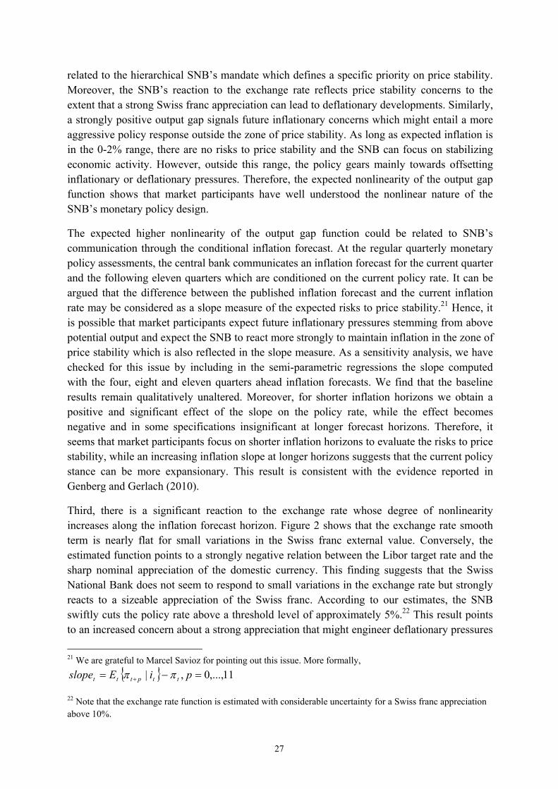
As pointed out in Genberg and Gerlach (2010), this evidence can be rationalized on the grounds of the SNB’s hierarchical mandate and the price stability definition which is formulated in terms of an inflation zone than as a specific numerical value. In a theoretical framework, Orphanides and Wieland (2000) show that if a central bank targets an inflation zone than a specific value, the optimal Taylor rule is nonlinear. The link to the Orphanides and Wieland paper is justified on the following grounds. First, the SNB does not target a specific inflation value. Its price stability definition is formulated in terms of an inflation range from 0 to 2%. Second, we find evidence for nonlinearity in the estimated rules. Hence, the observed nonlinearity of the estimated central bank and market-expected rules can be

27

related to the hierarchical SNB’s mandate which defines a specific priority on price stability. Moreover, the SNB’s reaction to the exchange rate reflects price stability concerns to the extent that a strong Swiss franc appreciation can lead to deflationary developments. Similarly, a strongly positive output gap signals future inflationary concerns which might entail a more aggressive policy response outside the zone of price stability. As long as expected inflation is in the 0-2% range, there are no risks to price stability and the SNB can focus on stabilizing economic activity. However, outside this range, the policy gears mainly towards offsetting inflationary or deflationary pressures. Therefore, the expected nonlinearity of the output gap function shows that market participants have well understood the nonlinear nature of the SNB’s monetary policy design.

The expected higher nonlinearity of the output gap function could be related to SNB’s communication through the conditional inflation forecast. At the regular quarterly monetary policy assessments, the central bank communicates an inflation forecast for the current quarter and the following eleven quarters which are conditioned on the current policy rate. It can be argued that the difference between the published inflation forecast and the current inflation rate may be considered as a slope measure of the expected risks to price stability.21 Hence, it is possible that market participants expect future inflationary pressures stemming from above potential output and expect the SNB to react more strongly to maintain inflation in the zone of price stability which is also reflected in the slope measure. As a sensitivity analysis, we have checked for this issue by including in the semi-parametric regressions the slope computed with the four, eight and eleven quarters ahead inflation forecasts. We find that the baseline results remain qualitatively unaltered. Moreover, for shorter inflation horizons we obtain a positive and significant effect of the slope on the policy rate, while the effect becomes negative and in some specifications insignificant at longer forecast horizons. Therefore, it seems that market participants focus on shorter inflation horizons to evaluate the risks to price stability, while an increasing inflation slope at longer horizons suggests that the current policy stance can be more expansionary. This result is consistent with the evidence reported in Genberg and Gerlach (2010).

Third, there is a significant reaction to the exchange rate whose degree of nonlinearity increases along the inflation forecast horizon. Figure 2 shows that the exchange rate smooth term is nearly flat for small variations in the Swiss franc external value. Conversely, the estimated function points to a strongly negative relation between the Libor target rate and the sharp nominal appreciation of the domestic currency. This finding suggests that the Swiss National Bank does not seem to respond to small variations in the exchange rate but strongly reacts to a sizeable appreciation of the Swiss franc. According to our estimates, the SNB swiftly cuts the policy rate above a threshold level of approximately 5%.22 This result points to an increased concern about a strong appreciation that might engineer deflationary pressures

21 We are grateful to Marcel Savioz for pointing out this issue. More formally,

11,...,0,| piEslope ttpttt

22 Note that the exchange rate function is estimated with considerable uncertainty for a Swiss franc appreciation above 10%.

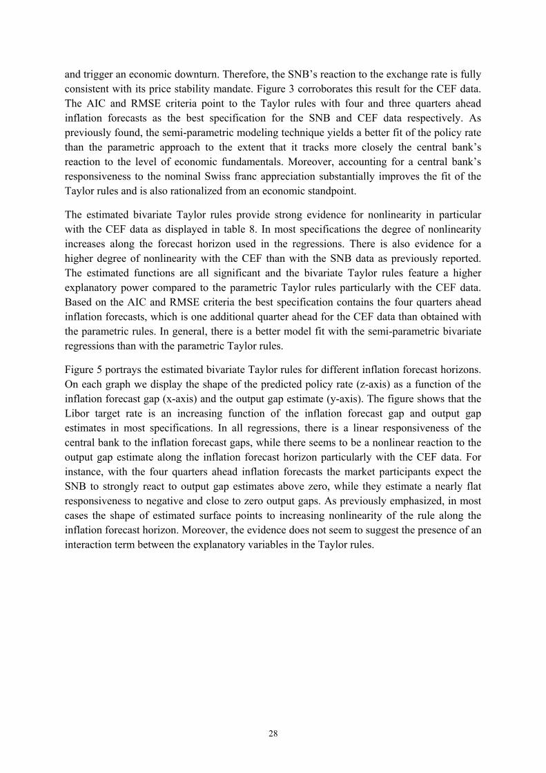
28

and trigger an economic downturn. Therefore, the SNB’s reaction to the exchange rate is fully consistent with its price stability mandate. Figure 3 corroborates this result for the CEF data. The AIC and RMSE criteria point to the Taylor rules with four and three quarters ahead inflation forecasts as the best specification for the SNB and CEF data respectively. As previously found, the semi-parametric modeling technique yields a better fit of the policy rate than the parametric approach to the extent that it tracks more closely the central bank’s reaction to the level of economic fundamentals. Moreover, accounting for a central bank’s responsiveness to the nominal Swiss franc appreciation substantially improves the fit of the Taylor rules and is also rationalized from an economic standpoint.

The estimated bivariate Taylor rules provide strong evidence for nonlinearity in particular with the CEF data as displayed in table 8. In most specifications the degree of nonlinearity increases along the forecast horizon used in the regressions. There is also evidence for a higher degree of nonlinearity with the CEF than with the SNB data as previously reported. The estimated functions are all significant and the bivariate Taylor rules feature a higher explanatory power compared to the parametric Taylor rules particularly with the CEF data. Based on the AIC and RMSE criteria the best specification contains the four quarters ahead inflation forecasts, which is one additional quarter ahead for the CEF data than obtained with the parametric rules. In general, there is a better model fit with the semi-parametric bivariate regressions than with the parametric Taylor rules.

Figure 5 portrays the estimated bivariate Taylor rules for different inflation forecast horizons. On each graph we display the shape of the predicted policy rate (z-axis) as a function of the inflation forecast gap (x-axis) and the output gap estimate (y-axis). The figure shows that the Libor target rate is an increasing function of the inflation forecast gap and output gap estimates in most specifications. In all regressions, there is a linear responsiveness of the central bank to the inflation forecast gaps, while there seems to be a nonlinear reaction to the output gap estimate along the inflation forecast horizon particularly with the CEF data. For instance, with the four quarters ahead inflation forecasts the market participants expect the SNB to strongly react to output gap estimates above zero, while they estimate a nearly flat responsiveness to negative and close to zero output gaps. As previously emphasized, in most cases the shape of estimated surface points to increasing nonlinearity of the rule along the inflation forecast horizon. Moreover, the evidence does not seem to suggest the presence of an interaction term between the explanatory variables in the Taylor rules.

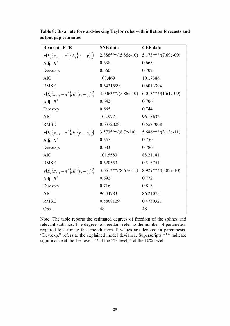
29

Table 8: Bivariate forward-looking Taylor rules with inflation forecasts and output gap estimates

Bivariate FTR SNB data CEF data **

1 , ttttt yyEEs 2.886***/(5.86e-10) 5.173***/(7.69e-09)

Adj. 2R 0.638 0.665

Dev.exp. 0.660 0.702

AIC 103.469 101.7386

RMSE 0.6421599 0.6013394 **

2 , ttttt yyEEs 3.006***/(5.86e-10) 6.013***/(1.61e-09)

Adj. 2R 0.642 0.706

Dev.exp. 0.665 0.744

AIC 102.9771 96.18632

RMSE 0.6372828 0.5577008 **

3 , ttttt yyEEs 3.573***/(8.7e-10) 5.686***/(3.13e-11)

Adj. 2R 0.657 0.750

Dev.exp. 0.683 0.780

AIC 101.5583 88.21181

RMSE 0.620553 0.516751 **

4 , ttttt yyEEs 3.651***/(8.67e-11) 8.929***/(3.82e-10)

Adj. 2R 0.692 0.772

Dev.exp. 0.716 0.816

AIC 96.34783 86.21075

RMSE 0.5868129 0.4730321

Obs. 48 48


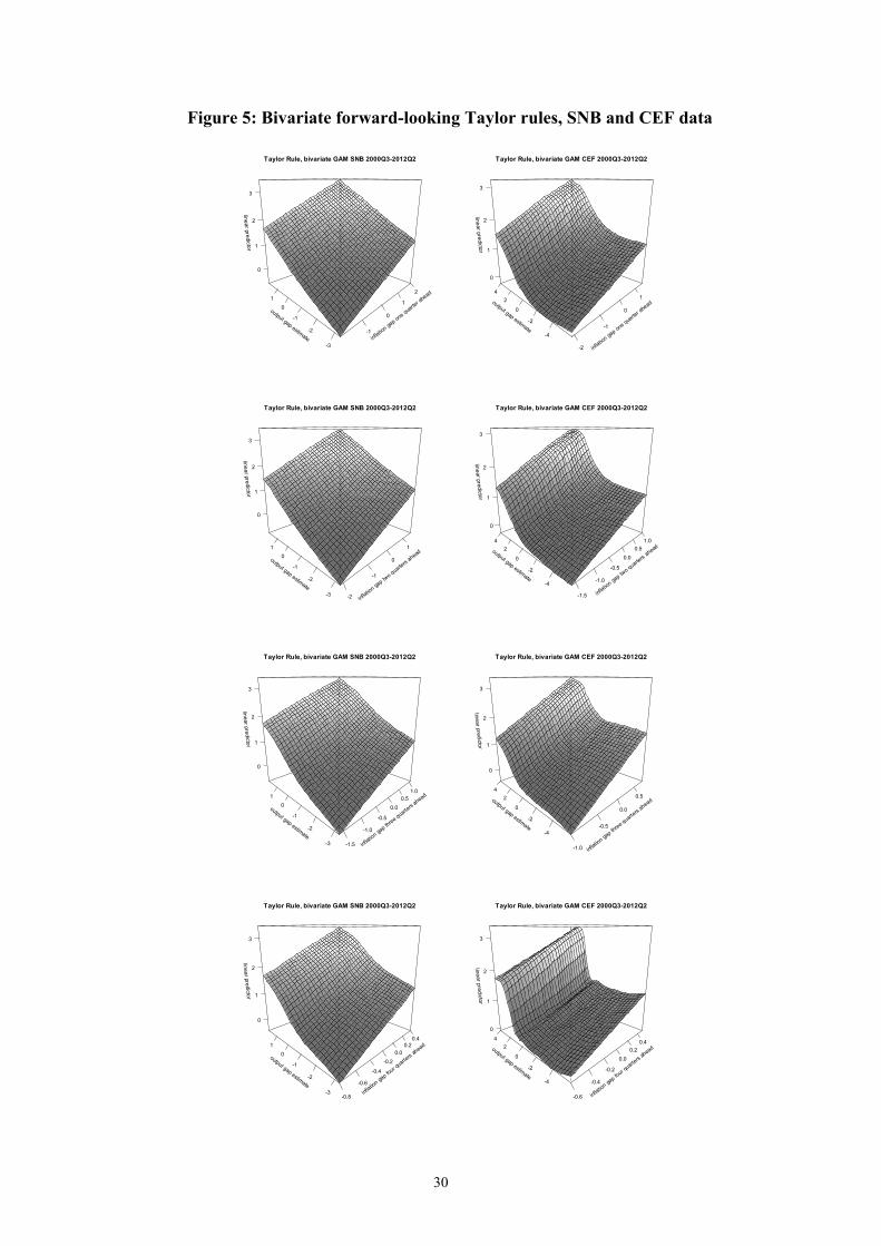
30

Figure 5: Bivariate forward-looking Taylor rules, SNB and CEF data

inflation gap one quarte

r ahead

-1

0

1

2

output gap estimate-3

-2

-1

01

linear predictor

0

1

2

3

Taylor Rule, bivariate GAM SNB 2000Q3-2012Q2

inflation gap one quarte

r ahead

-2

-1

0

1output gap estimate

-4

-2

0

24

linear predictor

0

1

2

3

Taylor Rule, bivariate GAM CEF 2000Q3-2012Q2

inflation gap two quarte

rsahead

-2

-1

0

1


-2

-1

01

linear predictor

0

1

2

3


inflation gap two quarte

rsahead

-1.5

-1.0

-0.5

0.00.5

1.0


-2

0

24

linear predictor

0

1

2

3


inflation gap three quarte

rs ahead

-1.5

-1.0

-0.5

0.00.5

1.0


-2

-1

01

linear predictor

0

1

2

3


inflation gap three quarte

rs ahead

-1.0

-0.5

0.0

0.5output gap estimate-4

-2

0

24

linear predictor

0

1

2

3


inflation gap four quarte

rsahead

-0.8

-0.6

-0.4

-0.20.0

0.20.4


-2

-1

01

linear predictor

0

1

2

3


inflation gap four quarte

rsahead

-0.6

-0.4

-0.2

0.00.2

0.4output gap estimate

-4

-2

0

24

linear predictor

0

1

2

3


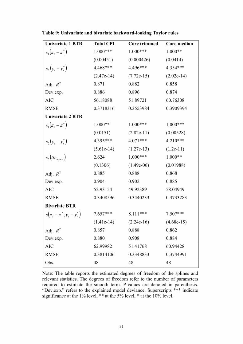
31

Table 9: Univariate and bivariate backward-looking Taylor rules

Univariate 1 BTR Total CPI Core trimmed Core median *

1 ts 1.000*** 1.000*** 1.000**

(0.00451) (0.000426) (0.0414) *

2 tt yys 4.468*** 4.496*** 4.354***

(2.47e-14) (7.72e-15) (2.02e-14)

Adj. 2R 0.871 0.882 0.858

Dev.exp. 0.886 0.896 0.874

AIC 56.18088 51.89721 60.76308

RMSE 0.3718316 0.3553984 0.3909394

Univariate 2 BTR *

1 ts 1.000** 1.000*** 1.000***

(0.0151) (2.82e-11) (0.00528) *

2 tt yys 4.395*** 4.071*** 4.210***

(5.61e-14) (1.27e-13) (1.2e-11)

tnomes ,3 2.624 1.000*** 1.000**

(0.1306) (1.49e-06) (0.01988)

Adj. 2R 0.885 0.888 0.868

Dev.exp. 0.904 0.902 0.885

AIC 52.93154 49.92389 58.04949

RMSE 0.3408596 0.3440233 0.3733283

Bivariate BTR **; ttt yys 7.657*** 8.111*** 7.507***

(1.41e-14) (2.24e-16) (4.68e-15)

Adj. 2R 0.857 0.888 0.862

Dev.exp. 0.880 0.908 0.884

AIC 62.99982 51.41768 60.94428

RMSE 0.3814106 0.3348833 0.3744991

Obs. 48 48 48


32

Finally, the semi-parametric backward-looking Taylor rules point to the presence of nonlinearities in particular with respect to the output gap and the exchange rate. The regression results are presented in table 9 and the estimated splines are displayed in figure 4. Most of the estimated smooth terms are significant and the RMSE point to a much closer fit of the policy rate with the semi-parametric Taylor rules than with the parametric specifications. The univariate rule without the exchange rate term indicates that the central bank’s reaction to inflation is linear while its responsiveness to the output gap is strongly nonlinear. This result thus corroborates the previous evidence obtained with the SNB and CEF forecasts. The specification with the exchange rate term confirms the earlier findings about the linearity of the inflation gap smooth term obtained with both the SNB and CEF data. The estimated output gap function suggests that the SNB reacts more strongly to positive output gaps to alleviate future inflationary pressures which is consistent with the previous results. In addition, the regressions corroborate the stronger reaction of the central bank to a substantial nominal effective Swiss franc appreciation with the total CPI measure. Nevertheless, this evidence is relatively mixed with the core inflation measures as the exchange rate terms are linear. The bivariate specifications show strong evidence for nonlinearity of the Taylor rule with the total CPI and the core inflation measures. In general, the univariate rules augmented with the exchange rate variable display a higher explanatory power and better in-sample fit than the parametric specifications and are preferred in light of the information criterion statistic.

To sum up, the evidence for nonlinearity with the semi-parametric regressions can be rationalized from the SNB’s hierarchical mandate. The central bank reacts more strongly to large variations in macroeconomic fundamentals to contain future inflationary pressures while it takes into account the developments of the economy. Along these lines, the SNB firmly responds to inflation, while its reaction to the output gap and to a nominal Swiss franc appreciation depends on the extent that these variables become a concern for price stability and economic activity. Therefore, the SNB’s reaction to the exchange rate is fully consistent with its price stability mandate.

7. Conclusion This paper provides new insights on understanding the SNB’s reaction to economic fundamentals in a Taylor rule framework based on internal macroeconomic forecasts and on the CEF measures of expectations. The empirical results point to the following main findings.

First, in line with the recent literature, there is strong evidence that the central bank’s reaction to inflation increases with the forecast horizon. Second, market participants seem to have well understood the SNB’s commitment to price stability as they have expected an even stronger policy reaction to inflation than found with the SNB’s internal ARIMA inflation forecasts and output gap estimates. Third, the best specification contains a reaction term to a Swiss franc appreciation along with the output gap estimate and the inflation forecasts four and three quarters ahead with the SNB and CEF data respectively. Finally, the semi-parametric regression results provide some empirical support for the nonlinear modeling of the Taylor rules. Notwithstanding a close to linear reaction to inflation there is clearly a nonlinear response to the output gap and the exchange rate.

33

The semi-parametric estimations suggest that the SNB has counteracted a strong Swiss franc appreciation possibly to prevent the emergence of an adverse feedback-loop from the exchange rate movements to prices and real economic activity. This policy responsiveness shows strong evidence for the SNB’s price stability commitment and accounts for a high level of inflation credibility. Nevertheless, market participants seem to have expected an even higher degree of nonlinearity in the Taylor rules than found with SNB internal data. This evidence may reflect a more cautious approach to modeling the expected rule on the part of the professional forecasters. They might face some degree of uncertainty regarding the SNB’s relative preferences for the key explanatory variables in the Taylor rules.

Future research should focus on assessing the forecasting performance of the semi-parametric Taylor rules out of the sample used for the estimations. In addition, on the grounds of a normative approach, we should study the optimality of Taylor rules within a specifically designed theoretical framework.

References Adam, C., Cobham, D. (2004). Real-time output gaps in the estimation of Taylor rules: a red herring? Oxford University Discussion Paper Series No. 218.

Alcidi, C., Flamini, A. & Fracasso, A. (2005). Taylored rules. Does one fit (or hide) all? HEI Working Paper No. 04/2005.

Alcidi, C., Flamini, A. & Fracasso, A. (2011). Policy Regime Changes, Judgment and Taylor rules in the Greenspan Era. Economica, 78, 89-107.

Andrews, D. (1993), Tests for Parameter Instability and Structural Change with Unknown Change Point. Econometrica, 61(4), 821-856.

Assenmacher-Wesche, K. (2006). Estimating Central Banks' preferences from a time-varying empirical reaction function. European Economic Review, 50(8), 1951-1974.

Bai, J., Perron P. (1998). Estimating and Testing Linear Models with Multiple Structural Changes. Econometrica, 66(1), 47-78.

Bai, J., Perron P. (2003). Computation and analysis of multiple structural change models. Journal of Applied Econometrics, 18, 1-22.

Baltensperger, E., Hildebrand, P.M., Jordan, T. J. (2007). The Swiss National Bank’s monetary policy concept- an example of a ‘principles-based’ policy framework. SNB Economic Studies No.03.

Batini, N., Haldane, A. (1999). Forward-Looking Rules for Monetary Policy. In J. B. Taylor, Monetary Policy Rules, 2001, (S. 157-192). Chicago: University of Chicago Press.

Batini, N., Harrison, R., & Millard, S. P. (2003). Monetary policy rules for an open economy. Journal of Economic Dynamics and Control, 27, 2059-2094.

34

Bäurle, G., Menz, T. (2008). Monetary policy in a small open economy model: A DSGE-VAR approach for Switzerland. Study Center Gerzensee Working Paper No. 08.03.

Chow, G.C. (1960). Tests of Equality Between Sets of Coefficients in Two Linear Regressions. Econometrica, 28(3), 591-605.

Clarida, R., Galí, J., & Gertler, M. (1998). Monetary Policy Rules in Practice: Some International Evidence. European Economic Review, 42(6), 1033-1067.

Clarida, R., Galí, J., & Gertler, M. (1999). The Science of Monetary Policy: A New Keynesian Perspective. Journal of Economic Literature, 37(4), 1661-1707.

Clarida, R., Galí, J., & Gertler, M. (2000). Monetary Policy Rules and Macroeconomic Stability: Evidence and Some Theory. Quarterly Journal of Economics, 115(1), 147-180.

Coibion, O., Gorodnichenko, Y. (2011). Why Are Target Interest Rate Changes So Persistent? NBER Working Paper No. 16707.

Conrad, C. Lamla, M. & Yu, K. (2010). Non-linear Taylor Rules. Preliminary Working Paper presented at the CIRET 2010 conference in New York.

Cuche, N. (2000). Monetary policy with forward looking rules: The Swiss case. Study Center Gerzensee Working Paper No. 00.10.

Cuche-Curti, N., Hall, P. & Zanetti, A. (2008). Swiss GDP revisions: A monetary policy perspective. Journal of Business Cycle Measurement and Analysis, 10(2), 183-213.

Galí, J. (2008). Monetary Policy, Inflation and the Business Cycle. An Introduction to the New Keynesian Framework. Princeton: Princeton University Press.

Genberg, H., Gerlach S. (2010). Swiss Monetary Policy 2000-2009. Swiss Journal of Economics and Statistics, 146(1), 131-165.

Gerdesmeier, D. Roffia, B. (2004). Taylor rules for the euro area: the issue of real-time data. Deutsche Bundesbank Discussion Paper No 37/2004.

Gerlach, S., Lewis, J. (2010). The Zero Lower Bound, ECB Interest Rate Policy and the Financial Crisis. De Nederlandsche Bank Working Paper No. 254.

Gorter, J., Jacobs, J. & de Haan J. (2008). Taylor Rules for the ECB using Expectations Data. Scandinavian Journal of Economics, 110(3), 473-488.

Hamilton, J.D., Pruitt, S. & Borger, S.C. (2009). The Market-Perceived Monetary Policy Rule. Federal Reserve Board, International Finance Discussion Paper No. 982.

Hansen, B.E. (2001). The New Econometrics of Structural Change: Dating Breaks in U.S. Labor Productivity. Journal of Economic Perspectives, 15(4), 117-128.

Hastie, T., Tibshirani, R. (1986). Generalized Additive Models (with discussion), Statistical Science 1(1), 297-318.

35

Hastie, T., Tibshirani, R. (1990). Generalized Additive Models, New York: Chapman and Hall.

Hayat, A., Mishra, S. (2010). Federal reserve monetary policy and the non-linearity of the Taylor rule. Economic Modelling, 27, 1292-1301.

Heppke-Falk, K., Hüfner, F. (2004). Expected budget deficits and interest rate swap spreads– Evidence for France, Germany and Italy. Deutsche Bundesbank Discussion Paper No. 40/2004.

Holmsen, A., Qvigstad, J. F., Roisland, O., & Solberg-Johansen, K. (2008). Communicating monetary policy intentions: The Case of Norges Bank. Norges Bank, Monetary Policy Department Working Paper No. 2008-20.

Huwiler, M., Kaufmann, D. (2013). Combining Disaggregate Forecasts for Inflation: The SNB’s ARIMA Model. SNB Economic Studies No. 7.

Jordan, T.J., Peytrignet, M. & Rossi, E. (2010). Ten Years’ Experience with the Swiss National Bank’s Monetary Policy Strategy. Swiss Journal of Economics and Statistics, 146(1), 9-90.

Kahn, G. A. (2012). Estimated Rules for Monetary Policy. Federal Reserve Bank of Kansas Economic Review, forthcoming.

Kim, Y-J., Gu, C. (2004). Smoothing Spline Gaussian Regression: More Scalable Computation via Efficient Approximation. Journal of the Royal Statistical Society, 66(2), 337-356.

Mankiw, N., Miron, J., & Weil, D. (1987). The Adjustment of Expectations to a Change in Regime: A Study of the Founding of the Federal Reserve. American Economic Review, 77(3),358-374.

Markov, N., de Porres, C. (2011). Is the Taylor rule nonlinear? Empirical evidence from a semi-parametric modeling approach. University of Geneva Working Paper No. 11052 and SSRN Working Paper No. 1854524.

Orphanides, A., Wieland V. (2000). Inflation Zone Targeting. European Economic Review, 44(7), 1351-1387.

Orphanides, A. (2001). Monetary Policy Rules Based on Real-Time Data. AmericanEconomic Review, 91(4), 964-985.

Orphanides, A., van Norden S. (2002). The unreliability of output-gap estimates in real-time. The Review of Economics and Statistics, 84(4), 569-583.

Owyang, M., Ramey, G. (2004). Regime Switching and Monetary Policy Measurement. Journal of Monetary Economics, 51(8), 1577-1597.

36

Perruchoud, A. (2009), Estimating a Taylor rule with Markov switching regimes for Switzerland. Swiss Journal of Economics and Statistics 145(2). 187-220.

Poplawski-Ribeiro, M., Rülke, J-C. (2011). Fiscal Expectations Under the Stability and Growth Pact. IMF Working Paper No. 11/48.

Rudebusch, G., Svensson, L. (1999). Policy Rules for Inflation Targeting. In J. B. Taylor, Monetary Policy Rules, 2001, (S. 203-246). Chicago: University of Chicago Press.

Rudebusch, G. (2002). Term Structure Evidence on Interest Rate Smoothing and Monetary Policy Inertia. Journal of Monetary Economics, 49(6), 1161-1187.

Rudebusch, G. (2006). Monetary Policy Inertia: Fact or Fiction? International Journal of Central Banking, 2(4), 85-135.

Sauer, S., Sturm, J-E. (2003). Using Taylor Rules to Understand ECB Monetary Policy. CES Ifo Working Paper No. 1110.

Sims, C., Zha, T. (2006). Were there Regime Switches in U.S. Monetary Policy? AmericanEconomic Review, 96(1), 54-81.

Svensson, L.E.O., (2003). What Is Wrong with Taylor Rules? Using Judgment in Monetary Policy through Targeting Rules. Journal of Economic Literature, 41(2), 426-477.

Taylor, J. B. (1993). Discretion versus policy rules in practice. Carnegie-RochesterConference Series on Public Policy 39, (S. 195-214).

Taylor, J. B. (2001). Monetary policy rules. National Bureau of Economic Research. Chicago : University of Chicago Press.

Taylor, J. B., Wieland, V. (2009). Surprising comparative properties of monetary models: results from a new data base. NBER Working Paper No. 14849.

Walsh, C. E. (2003). Speed Limit Policies: The Output Gap and Optimal Monetary Policy. American Economic Review , 93(1), 265-278.

Wood, S. N. (2006). Generalized Additive Models. An introduction with R. New York: Chapman and Hall.

Woodford, M. (2003). Interest and Prices. Foundations of a Theory of Monetary Policy.Princeton: Princeton University Press.

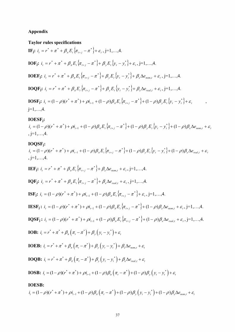
37

Appendix

Taylor rules specifications

IFj: tjttt Eri *** , j=1,…,4.

IOFj: ttttyjttt yyEEri **** , j=1,…,4.

IOEFj: ttnometttyjttt eyyEEri ,**** , j=1,…,4.

IOQFj: ttrealetttyjttt eyyEEri ,**** , j=1,…,4.

IOSFj: ttttyjtttt yyEEiri **1

** )1()1())(1( ,

j=1,…,4.

IOESFj:

ttnometttyjtttt eyyEEiri ,**

1** )1()1()1())(1(

, j=1,…,4.

IOQSFj:

ttrealetttyjtttt eyyEEiri ,**

1** )1()1()1())(1(

, j=1,…,4.

IEFj: ttnomejttt eEri ,*** , j=1,…,4.

IQFj: ttrealejttt eEri ,*** , j=1,…,4.

ISFj: tjtttt Eiri *1

** )1())(1( , j=1,…,4.

IESFj : ttnomejtttt eEiri ,*

1** )1()1())(1( , j=1,…,4.

IQSFj : ttrealejtttt eEiri ,*

1** )1()1())(1( , j=1,…,4.

IOB: * * * *t t y t t ti r y y

IOEB: * * * *,t t y t t e nom t ti r y y e

IOQB: * * * *,t t y t t e real t ti r y y e

IOSB: * * * *1(1 )( ) (1 ) (1 )t t t y t t ti r i y y

IOESB:* * * *

1 ,(1 )( ) (1 ) (1 ) (1 )t t t y t t e nom t ti r i y y e

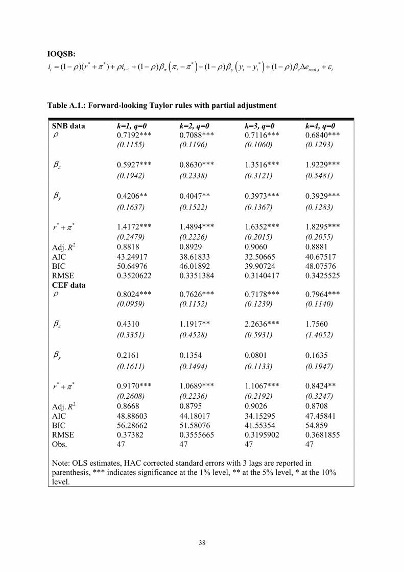
38

IOQSB:* * * *

1 ,(1 )( ) (1 ) (1 ) (1 )t t t y t t e real t ti r i y y e

Table A.1.: Forward-looking Taylor rules with partial adjustment

SNB data k=1, q=0 k=2, q=0 k=3, q=0 k=4, q=0 0.7192*** 0.7088*** 0.7116*** 0.6840*** (0.1155) (0.1196) (0.1060) (0.1293) 0.5927*** 0.8630*** 1.3516*** 1.9229*** (0.1942) (0.2338) (0.3121) (0.5481)

y 0.4206** 0.4047** 0.3973*** 0.3929*** (0.1637) (0.1522) (0.1367) (0.1283)

* *r 1.4172*** 1.4894*** 1.6352*** 1.8295*** (0.2479) (0.2226) (0.2015) (0.2055)

Adj. 2R 0.8818 0.8929 0.9060 0.8881 AIC BIC

43.2491750.64976

38.6183346.01892

32.5066539.90724

40.6751748.07576

RMSE 0.3520622 0.3351384 0.3140417 0.3425525 CEF data

0.8024*** 0.7626*** 0.7178*** 0.7964*** (0.0959) (0.1152) (0.1239) (0.1140) 0.4310 1.1917** 2.2636*** 1.7560 (0.3351) (0.4528) (0.5931) (1.4052)

y 0.2161 0.1354 0.0801 0.1635 (0.1611) (0.1494) (0.1133) (0.1947)

* *r 0.9170*** 1.0689*** 1.1067*** 0.8424** (0.2608) (0.2236) (0.2192) (0.3247)

Adj. 2R 0.8668 0.8795 0.9026 0.8708 AIC BIC

48.8860356.28662

44.1801751.58076

34.1529541.55354

47.4584154.859

RMSE 0.37382 0.3555665 0.3195902 0.3681855 Obs. 47 47 47 47 Note: OLS estimates, HAC corrected standard errors with 3 lags are reported in parenthesis, *** indicates significance at the 1% level, ** at the 5% level, * at the 10% level.

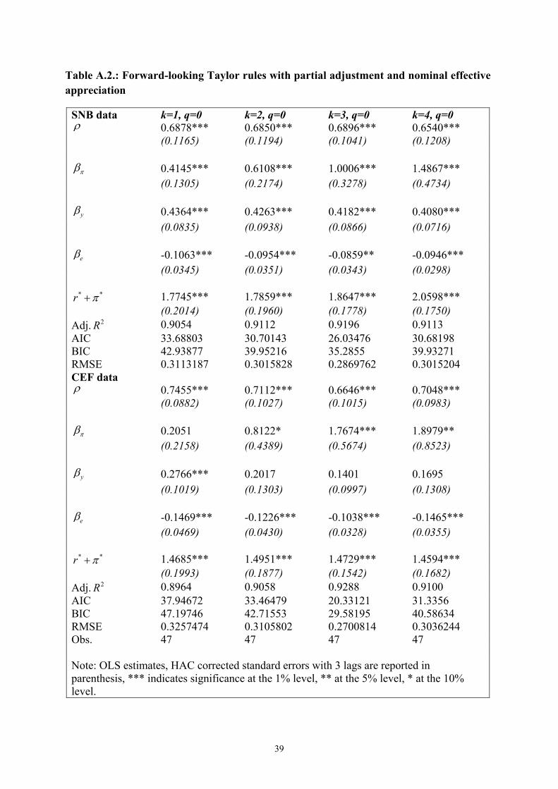
39

Table A.2.: Forward-looking Taylor rules with partial adjustment and nominal effective appreciation


0.4145*** 0.6108*** 1.0006*** 1.4867*** (0.1305) (0.2174) (0.3278) (0.4734)

y 0.4364*** 0.4263*** 0.4182*** 0.4080*** (0.0835) (0.0938) (0.0866) (0.0716)

e -0.1063*** -0.0954*** -0.0859** -0.0946*** (0.0345) (0.0351) (0.0343) (0.0298)

* *r 1.7745*** 1.7859*** 1.8647*** 2.0598*** (0.2014) (0.1960) (0.1778) (0.1750)

Adj. 2R 0.9054 0.9112 0.9196 0.9113 AIC BIC

33.6880342.93877

30.7014339.95216

26.0347635.2855

30.6819839.93271

RMSE 0.3113187 0.3015828 0.2869762 0.3015204 CEF data

0.7455*** 0.7112*** 0.6646*** 0.7048*** (0.0882) (0.1027) (0.1015) (0.0983)

0.2051 0.8122* 1.7674*** 1.8979** (0.2158) (0.4389) (0.5674) (0.8523)

y 0.2766*** 0.2017 0.1401 0.1695 (0.1019) (0.1303) (0.0997) (0.1308)

e -0.1469*** -0.1226*** -0.1038*** -0.1465*** (0.0469) (0.0430) (0.0328) (0.0355)

* *r 1.4685*** 1.4951*** 1.4729*** 1.4594*** (0.1993) (0.1877) (0.1542) (0.1682)

Adj. 2R 0.8964 0.9058 0.9288 0.9100 AIC BIC

37.9467247.19746

33.4647942.71553

20.3312129.58195

31.335640.58634

RMSE 0.3257474 0.3105802 0.2700814 0.3036244 Obs. 47 47 47 47 Note: OLS estimates, HAC corrected standard errors with 3 lags are reported in parenthesis, *** indicates significance at the 1% level, ** at the 5% level, * at the 10% level.

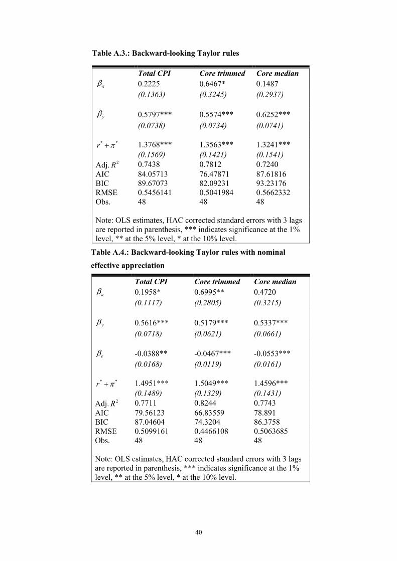
40

Table A.3.: Backward-looking Taylor rules

Total CPI Core trimmed Core median 0.2225 0.6467* 0.1487 (0.1363) (0.3245) (0.2937)

y 0.5797*** 0.5574*** 0.6252*** (0.0738) (0.0734) (0.0741)

* *r 1.3768*** 1.3563*** 1.3241*** (0.1569) (0.1421) (0.1541)

Adj. 2R 0.7438 0.7812 0.7240 AIC BIC

84.0571389.67073

76.4787182.09231

87.6181693.23176

RMSE 0.5456141 0.5041984 0.5662332 Obs. 48 48 48 Note: OLS estimates, HAC corrected standard errors with 3 lags are reported in parenthesis, *** indicates significance at the 1% level, ** at the 5% level, * at the 10% level.

Table A.4.: Backward-looking Taylor rules with nominal effective appreciation

Total CPI Core trimmed Core median 0.1958* 0.6995** 0.4720 (0.1117) (0.2805) (0.3215)

y 0.5616*** 0.5179*** 0.5337*** (0.0718) (0.0621) (0.0661)

e -0.0388** -0.0467*** -0.0553*** (0.0168) (0.0119) (0.0161)

* *r 1.4951*** 1.5049*** 1.4596*** (0.1489) (0.1329) (0.1431)

Adj. 2R 0.7711 0.8244 0.7743 AIC BIC

79.5612387.04604

66.8355974.3204

78.89186.3758


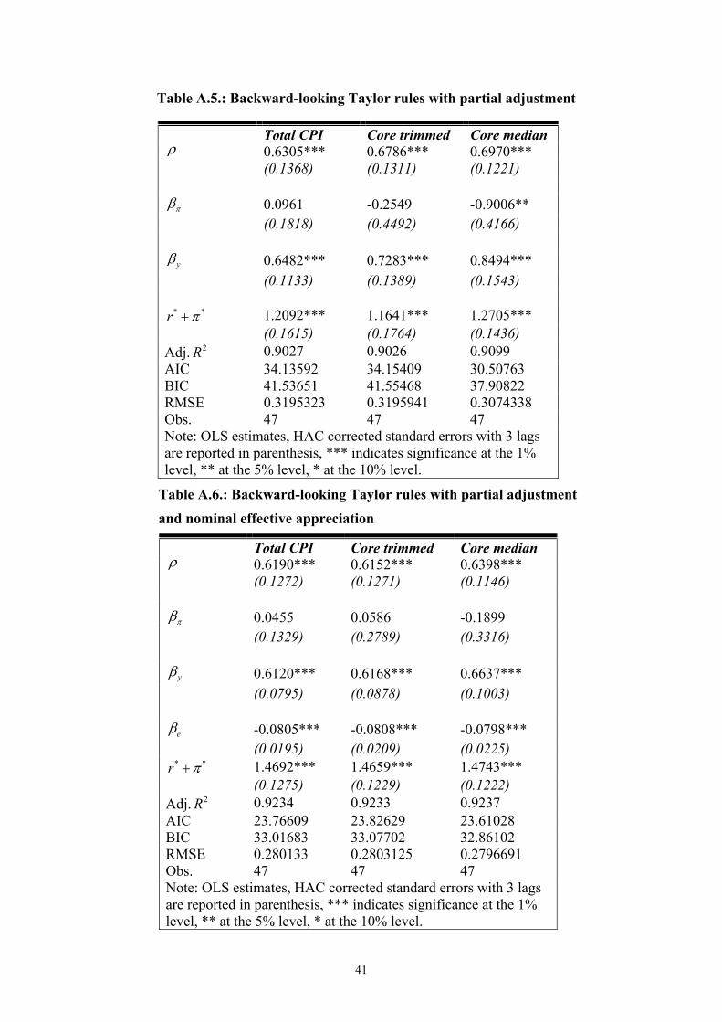
41

Table A.5.: Backward-looking Taylor rules with partial adjustment

Total CPI Core trimmed Core median 0.6305*** 0.6786*** 0.6970***

(0.1368) (0.1311) (0.1221)

0.0961 -0.2549 -0.9006** (0.1818) (0.4492) (0.4166)

y 0.6482*** 0.7283*** 0.8494*** (0.1133) (0.1389) (0.1543)

* *r 1.2092*** 1.1641*** 1.2705*** (0.1615) (0.1764) (0.1436) Adj. 2R 0.9027 0.9026 0.9099 AIC BIC

34.1359241.53651

34.1540941.55468

30.5076337.90822


Table A.6.: Backward-looking Taylor rules with partial adjustment and nominal effective appreciation

Total CPI Core trimmed Core median 0.6190*** 0.6152*** 0.6398*** (0.1272) (0.1271) (0.1146) 0.0455 0.0586 -0.1899 (0.1329) (0.2789) (0.3316)

y 0.6120*** 0.6168*** 0.6637*** (0.0795) (0.0878) (0.1003)

e -0.0805*** -0.0808*** -0.0798*** (0.0195) (0.0209) (0.0225)

* *r 1.4692*** 1.4659*** 1.4743*** (0.1275) (0.1229) (0.1222)

Adj. 2R 0.9234 0.9233 0.9237 AIC 23.76609 23.82629 23.61028 BIC 33.01683 33.07702 32.86102 RMSE 0.280133 0.2803125 0.2796691 Obs. 47 47 47 Note: OLS estimates, HAC corrected standard errors with 3 lags are reported in parenthesis, *** indicates significance at the 1% level, ** at the 5% level, * at the 10% level.

Swiss National Bank Working Papers published since 2004: 2004-1 Samuel Reynard: Financial Market Participation and the Apparent Instability of

Money Demand 2004-2 Urs W. Birchler and Diana Hancock: What Does the Yield on Subordinated Bank Debt Measure? 2005-1 Hasan Bakhshi, Hashmat Khan and Barbara Rudolf: The Phillips curve under state-dependent pricing 2005-2 Andreas M. Fischer: On the Inadequacy of Newswire Reports for Empirical Research on Foreign Exchange Interventions 2006-1 Andreas M. Fischer: Measuring Income Elasticity for Swiss Money Demand: What do the Cantons say about Financial Innovation? 2006-2 Charlotte Christiansen and Angelo Ranaldo: Realized Bond-Stock Correlation:

Macroeconomic Announcement Effects 2006-3 Martin Brown and Christian Zehnder: Credit Reporting, Relationship Banking, and Loan Repayment 2006-4 Hansjörg Lehmann and Michael Manz: The Exposure of Swiss Banks to

Macroeconomic Shocks – an Empirical Investigation 2006-5 Katrin Assenmacher-Wesche and Stefan Gerlach: Money Growth, Output Gaps and

Inflation at Low and High Frequency: Spectral Estimates for Switzerland 2006-6 Marlene Amstad and Andreas M. Fischer: Time-Varying Pass-Through from Import

Prices to Consumer Prices: Evidence from an Event Study with Real-Time Data 2006-7 Samuel Reynard: Money and the Great Disinflation 2006-8 Urs W. Birchler and Matteo Facchinetti: Can bank supervisors rely on market data?

A critical assessment from a Swiss perspective 2006-9 Petra Gerlach-Kristen: A Two-Pillar Phillips Curve for Switzerland 2006-10 Kevin J. Fox and Mathias Zurlinden: On Understanding Sources of Growth and

Output Gaps for Switzerland 2006-11 Angelo Ranaldo: Intraday Market Dynamics Around Public Information Arrivals 2007-1 Andreas M. Fischer, Gulzina Isakova and Ulan Termechikov: Do FX traders in

Bishkek have similar perceptions to their London colleagues? Survey evidence of market practitioners’ views

2007-2 Ibrahim Chowdhury and Andreas Schabert: Federal Reserve Policy viewed through a Money Supply Lens

2007-3 Angelo Ranaldo: Segmentation and Time-of-Day Patterns in Foreign Exchange

Markets 2007-4 Jürg M. Blum: Why ‘Basel II’ May Need a Leverage Ratio Restriction 2007-5 Samuel Reynard: Maintaining Low Inflation: Money, Interest Rates, and Policy

Stance 2007-6 Rina Rosenblatt-Wisch: Loss Aversion in Aggregate Macroeconomic Time Series 2007-7 Martin Brown, Maria Rueda Maurer, Tamara Pak and Nurlanbek Tynaev: Banking

Sector Reform and Interest Rates in Transition Economies: Bank-Level Evidence from Kyrgyzstan

2007-8 Hans-Jürg Büttler: An Orthogonal Polynomial Approach to Estimate the Term

Structure of Interest Rates 2007-9 Raphael Auer: The Colonial Origins Of Comparative Development: Comment.

A Solution to the Settler Mortality Debate

2007-10 Franziska Bignasca and Enzo Rossi: Applying the Hirose-Kamada filter to Swiss data: Output gap and exchange rate pass-through estimates

2007-11 Angelo Ranaldo and Enzo Rossi: The reaction of asset markets to Swiss National

Bank communication 2007-12 Lukas Burkhard and Andreas M. Fischer: Communicating Policy Options at the Zero

Bound 2007-13 Katrin Assenmacher-Wesche, Stefan Gerlach, and Toshitaka Sekine: Monetary

Factors and Inflation in Japan 2007-14 Jean-Marc Natal and Nicolas Stoffels: Globalization, markups and the natural rate

of interest 2007-15 Martin Brown, Tullio Jappelli and Marco Pagano: Information Sharing and Credit:

Firm-Level Evidence from Transition Countries 2007-16 Andreas M. Fischer, Matthias Lutz and Manuel Wälti: Who Prices Locally? Survey

Evidence of Swiss Exporters 2007-17 Angelo Ranaldo and Paul Söderlind: Safe Haven Currencies

2008-1 Martin Brown and Christian Zehnder: The Emergence of Information Sharing in Credit Markets

2008-2 Yvan Lengwiler and Carlos Lenz: Intelligible Factors for the Yield Curve 2008-3 Katrin Assenmacher-Wesche and M. Hashem Pesaran: Forecasting the Swiss

Economy Using VECX* Models: An Exercise in Forecast Combination Across Models and Observation Windows

2008-4 Maria Clara Rueda Maurer: Foreign bank entry, institutional development and

credit access: firm-level evidence from 22 transition countries 2008-5 Marlene Amstad and Andreas M. Fischer: Are Weekly Inflation Forecasts

Informative? 2008-6 Raphael Auer and Thomas Chaney: Cost Pass Through in a Competitive Model of

Pricing-to-Market 2008-7 Martin Brown, Armin Falk and Ernst Fehr: Competition and Relational Contracts:

The Role of Unemployment as a Disciplinary Device 2008-8 Raphael Auer: The Colonial and Geographic Origins of Comparative Development 2008-9 Andreas M. Fischer and Angelo Ranaldo: Does FOMC News Increase Global FX

Trading? 2008-10 Charlotte Christiansen and Angelo Ranaldo: Extreme Coexceedances in New EU

Member States’ Stock Markets

2008-11 Barbara Rudolf and Mathias Zurlinden: Measuring capital stocks and capital services in Switzerland

2008-12 Philip Sauré: How to Use Industrial Policy to Sustain Trade Agreements 2008-13 Thomas Bolli and Mathias Zurlinden: Measuring growth of labour quality and the

quality-adjusted unemployment rate in Switzerland 2008-14 Samuel Reynard: What Drives the Swiss Franc? 2008-15 Daniel Kaufmann: Price-Setting Behaviour in Switzerland – Evidence from CPI

Micro Data

2008-16 Katrin Assenmacher-Wesche and Stefan Gerlach: Financial Structure and the Impact of Monetary Policy on Asset Prices

2008-17 Ernst Fehr, Martin Brown and Christian Zehnder: On Reputation: A

Microfoundation of Contract Enforcement and Price Rigidity

2008-18 Raphael Auer and Andreas M. Fischer: The Effect of Low-Wage Import Competition on U.S. Inflationary Pressure

2008-19 Christian Beer, Steven Ongena and Marcel Peter: Borrowing in Foreign Currency:

Austrian Households as Carry Traders

2009-1 Thomas Bolli and Mathias Zurlinden: Measurement of labor quality growth caused by unobservable characteristics

2009-2 Martin Brown, Steven Ongena and Pinar Ye,sin: Foreign Currency Borrowing by

Small Firms 2009-3 Matteo Bonato, Massimiliano Caporin and Angelo Ranaldo: Forecasting realized

(co)variances with a block structure Wishart autoregressive model 2009-4 Paul Söderlind: Inflation Risk Premia and Survey Evidence on Macroeconomic

Uncertainty 2009-5 Christian Hott: Explaining House Price Fluctuations 2009-6 Sarah M. Lein and Eva Köberl: Capacity Utilisation, Constraints and Price

Adjustments under the Microscope 2009-7 Philipp Haene and Andy Sturm: Optimal Central Counterparty Risk Management 2009-8 Christian Hott: Banks and Real Estate Prices 2009-9 Terhi Jokipii and Alistair Milne: Bank Capital Buffer and Risk

Adjustment Decisions

2009-10 Philip Sauré: Bounded Love of Variety and Patterns of Trade 2009-11 Nicole Allenspach: Banking and Transparency: Is More Information

Always Better?

2009-12 Philip Sauré and Hosny Zoabi: Effects of Trade on Female Labor Force Participation 2009-13 Barbara Rudolf and Mathias Zurlinden: Productivity and economic growth in

Switzerland 1991-2005 2009-14 Sébastien Kraenzlin and Martin Schlegel: Bidding Behavior in the SNB's Repo

Auctions 2009-15 Martin Schlegel and Sébastien Kraenzlin: Demand for Reserves and the Central

Bank's Management of Interest Rates 2009-16 Carlos Lenz and Marcel Savioz: Monetary determinants of the Swiss franc

2010-1 Charlotte Christiansen, Angelo Ranaldo and Paul Söderlind: The Time-Varying Systematic Risk of Carry Trade Strategies

2010-2 Daniel Kaufmann: The Timing of Price Changes and the Role of Heterogeneity 2010-3 Loriano Mancini, Angelo Ranaldo and Jan Wrampelmeyer: Liquidity in the Foreign

Exchange Market: Measurement, Commonality, and Risk Premiums 2010-4 Samuel Reynard and Andreas Schabert: Modeling Monetary Policy 2010-5 Pierre Monnin and Terhi Jokipii: The Impact of Banking Sector Stability on the

Real Economy 2010-6 Sébastien Kraenzlin and Thomas Nellen: Daytime is money 2010-7 Philip Sauré: Overreporting Oil Reserves 2010-8 Elizabeth Steiner: Estimating a stock-flow model for the Swiss housing market 2010-9 Martin Brown, Steven Ongena, Alexander Popov, and Pinar Ye,sin: Who Needs

Credit and Who Gets Credit in Eastern Europe? 2010-10 Jean-Pierre Danthine and André Kurmann: The Business Cycle Implications of

Reciprocity in Labor Relations 2010-11 Thomas Nitschka: Momentum in stock market returns: Implications for risk premia

on foreign currencies 2010-12 Petra Gerlach-Kristen and Barbara Rudolf: Macroeconomic and interest rate

volatility under alternative monetary operating procedures 2010-13 Raphael Auer: Consumer Heterogeneity and the Impact of Trade Liberalization:

How Representative is the Representative Agent Framework? 2010-14 Tommaso Mancini Griffoli and Angelo Ranaldo: Limits to arbitrage during the

crisis: funding liquidity constraints and covered interest parity 2010-15 Jean-Marc Natal: Monetary Policy Response to Oil Price Shocks 2010-16 Kathrin Degen and Andreas M. Fischer: Immigration and Swiss House Prices 2010-17 Andreas M. Fischer: Immigration and large banknotes 2010-18 Raphael Auer: Are Imports from Rich Nations Deskilling Emerging Economies?

Human Capital and the Dynamic Effects of Trade

2010-19 Jean-Pierre Danthine and John B. Donaldson: Executive Compensation: A General Equilibrium Perspective

2011-1 Thorsten Beck and Martin Brown: Which Households Use Banks? Evidence from the

Transition Economies 2011-2 Martin Brown, Karolin Kirschenmann and Steven Ongena: Foreign Currency Loans –

Demand or Supply Driven? 2011-3 Victoria Galsband and Thomas Nitschka: Foreign currency returns and systematic

risks 2011-4 Francis Breedon and Angelo Ranaldo: Intraday patterns in FX returns and order

flow 2011-5 Basil Guggenheim, Sébastien Kraenzlin and Silvio Schumacher: Exploring an

uncharted market: Evidence on the unsecured Swiss franc money market 2011-6 Pamela Hall: Is there any evidence of a Greenspan put? 2011-7 Daniel Kaufmann and Sarah Lein: Sectoral Inflation Dynamics, Idiosyncratic

Shocks and Monetary Policy 2011-8 Iva Cecchin: Mortgage Rate Pass-Through in Switzerland 2011-9 Raphael A. Auer, Kathrin Degen and Andreas M. Fischer: Low-Wage Import

Competition, Inflationary Pressure, and Industry Dynamics in Europe 2011-10 Raphael A. Auer and Philip Sauré: Spatial Competition in Quality, Demand-Induced

Innovation, and Schumpeterian Growth 2011-11 Massimiliano Caporin , Angelo Ranaldo and Paolo Santucci de Magistris: On the

Predictability of Stock Prices: a Case for High and Low Prices 2011-12 Jürg Mägerle and Thomas Nellen: Interoperability between central counterparties 2011-13 Sylvia Kaufmann: K-state switching models with endogenous transition

distributions 2011-14 Sébastien Kraenzlin and Benedikt von Scarpatetti: Bargaining Power in the Repo

Market 2012-01 Raphael A. Auer: Exchange Rate Pass-Through, Domestic Competition, and

Inflation: Evidence from the 2005/08 Revaluation of the Renminbi 2012-02 Signe Krogstrup, Samuel Reynard and Barbara Sutter: Liquidity Effects of

Quantitative Easing on Long-Term Interest Rates

2012-03 Matteo Bonato, Massimiliano Caporin and Angelo Ranaldo: Risk spillovers in international equity portfolios

2012-04 Thomas Nitschka: Banking sectors’ international interconnectedness: Implications

for consumption risk sharing in Europe 2012-05 Martin Brown, Steven Ongena and Pinar Ye in: Information Asymmetry and

Foreign Currency Borrowing by Small Firms 2012-06 Philip Sauré and Hosny Zoabi: Retirement Age across Countries: The Role of

Occupations 2012-07 Christian Hott and Terhi Jokipii: Housing Bubbles and Interest Rates 2012-08 Romain Baeriswyl and Camille Cornand: Reducing overreaction to central bank’s

disclosures: theory and experiment 2012-09 Bo E. Honoré, Daniel Kaufmann and Sarah Lein: Asymmetries in Price-Setting

Behavior: New Microeconometric Evidence from Switzerland 2012-10 Thomas Nitschka: Global and country-specific business cycle risk in time-varying

excess returns on asset markets 2012-11 Raphael A. Auer, Thomas Chaney and Philip Sauré: Quality Pricing-to-Market 2012-12 Sébastien Kraenzlin and Thomas Nellen: Access policy and money market

segmentation 2012-13 Andreas Kropf and Philip Sauré: Fixed Costs per Shipment 2012-14 Raphael A. Auer and Raphael S. Schoenle: Market Structure and Exchange Rate

Pass-Through 2012-15 Raphael A. Auer: What Drives Target2 Balances? Evidence From a Panel Analysis 2012-16 Katja Drechsel and Rolf Scheufele: Bottom-up or Direct? Forecasting German GDP

in a Data-rich Environment 2013-01 Andreas Kettemann and Signe Krogstrup: Portfolio balance effects of the SNB’s

bond purchase program 2013-02 Nicole Aregger, Martin Brown and Enzo Rossi: Transaction Taxes, Capital Gains

Taxes and House Prices 2013-03 Simone Meier: Financial Globalization and Monetary Transmission

2013-04 Christian Grisse and Thomas Nitschka: On financial risk and the safe haven characteristics of Swiss franc exchange rates

2013-05 Matthias Gubler and Matthias S. Hertweck: Commodity Price Shocks and the

Business Cycle: Structural Evidence for the U.S. 2013-06 Elisabeth Beusch, Barbara Döbeli, Andreas Fischer and P nar Ye in: Merchanting

and Current Account Balances 2013-07 Victoria Galsband and Thomas Nitschka: Currency excess returns and global

downside market risk 2013-08 Nikolay Markov and Thomas Nitschka: Estimating Taylor Rules for Switzerland:

Evidence from 2000 to 2012

Swiss National Bank Working Papers are also available at www.snb.ch, section Publications/ResearchSubscriptions or individual issues can be ordered at Swiss National Bank, Fraumünsterstrasse 8, CH-8022 Zurich, fax +41 44 631 81 14, E-mail [email protected]

Documents

Swiss National Bank Working Papers · 2013-8 Swiss National Bank Working Papers Estimating Taylor Rules for Switzerland: Evidence from 2000 to 2012 Nikolay Markov and Thomas Nitschka