Survival and Event History Modelsvia Gamma Processes

Nils Lid Hjort (with Celine Cunen)

Department of Mathematics, University of Oslo

FocuStat VVV Conference, May 2018

1/1001

Process to Model:

2/1001

General themes

All models are wrong – but some are biologically more plausiblethan others.

Hope: construction of good models (and then methods) for hazardrates, for survival and event history data, for competing risks, etc.

I Cox model: some non-coherency issues

I Frailty modelling =⇒ classes of hazard rate models

I Bayesian nonparametrics =⇒ classes of hazard rate models

I Cumulative damage process reaches threshold =⇒ models

I Survival as long as all shocks are small =⇒ models

I Parallel damage processes =⇒ competing risks models

I Some damage process never reach threshold =⇒ cure models

I When ‘event’ is time related =⇒ extended logistic regression

3/1001

Plan

0 The incoherence of Cox; frailty and cumulative damageprocesses =⇒ models

1 Gamma process time-to-hit =⇒ models

2 Applications A, B, C

3 Gamma process jumps =⇒ models

4 Extended logistic regression (with brief application)

5 Competing risks (with brief application)

6 Frailtifying the threshold model

7 Concluding remarks

4/1001

0: Issues with Cox type models

Consider survival data with two covariates x1 and x2. Coxregression takes hazard to be

h(s | xi ,1, xi ,2) = h0(s) exp(β1xi ,1 + β2xi ,2).

There is a model-inconsistency problem here: if we only observexi ,1, and calculate the hazard rate h(s | xi ,1), then this will not beof Cox regression form, regardless of distribution of x2 | x1.

Also: if there is perfect Cox structure given x1 alone, and perfectCox structure given x2 alone, one almost never has a Cox model in(x1, x2).

Hence: the Cox model suffers from a coherence or plausibilityproblem. Important: finding good, biologically plausiblebackground explanations that actually imply the Cox structure (orother structures).

5/1001

Frailty processes

There is a broad literature on frailty in survival analysis. These areunobservable or latent explanatory variables accounting forrisk-differences between individuals.

In Aalen and NLH (2002):

I some classes of frailty variables, derived via Levy processes,imply Cox structure;

I some classes of frailty processes also imply Cox structure.

Assume that individual i has covariate xi and an associated frailtyprocess Zi (t), growing in time, such that

S(t | xi ,Zi ) = Pr{Ti > t | xi ,Zi ) = exp{−Zi (t)}.

Different models for (the invisible) Zi (·) lead to different models for

S(t | xi ) = Pr{Ti > t | xi} = E exp{−Zi (t)}.

6/1001

Cumulative damage processes

Take in particular

Zi (t) =∑

j≤Mi (t)

θiGi ,j ,

where Mi (·) is a Poisson process with rate λi (·) and the Gi ,j arei.i.d., as in cumulative shock model. Then

S(t | xi ,Zi ) =∏

j≤Mi (t)

exp(−θiGi ,j),

leading to

S(t | xi ) = E L0(θi )Mi (t) = exp[−Λi (t){1− L0(θi )}].

Here L0(θi ) = E exp(−θiGi ,j) is the Laplace transform of the Gi ,j ,and Λi (t) =

∫ t0 λi (s) ds.

Different models for λi (s), for θi and Gi ,j , in terms of the covariatexi , yield hazard rate regression models, via

h(s | xi ) = λi (s){1− E exp(−θiGi )}.7/1001

Among many possibilities: θi constant over individuals; Gi samedistribution across individuals; and λi (s) as in multiplicativePoisson regression, with λ0(s) exp(x ti β). This frailty processconstruction then implies the Cox structure:

h(s | xi ) = λ0(s) exp(x ti β){1− E exp(−θG )}.

Competing models also emerge naturally. Among them:

h(s | xi ) = λ0(s) exp(x ti β)exp(x ti γ)

1 + exp(x ti γ),

e.g. De Blasi and Hjort (2007). Also: additive regression models,via additive model for Poisson rate.

‘Twin times’ models, via frailty processes

Z0(t) + Z1(t) and Z0(t) + Z2(t).

These have convenient joint Laplace transforms.

8/1001

1: Time-to-hit models

Time-to-hit-threshold models: Frailty process considerations alsoinspire non-Cox regression models. Let

Ti = min{t ≥ 0: Zi (t) ≥ ci}

whereZi (t) ∼ Gam(aMi (t), 1) a Gamma process.

Then

Si (t) = Pr{Ti ≥ t} = Pr{Zi (t) < ci}

= G (ci , aMi (t), 1) =

∫ ci

0g(x , aMi (t), 1)dx .

This is a large class of models, with many shapes for hazards hi (t),depending on Mi and size of ci . With acceleration factorsG (c , aM(κi t)) we may have crossing hazards.

9/1001

Thus the nonparametric process view generates fresh regressionmodels (parametric, semiparametric or nonparametric).

One version: as above, with regression on both threshold andacceleration:

Zi (t) ∼ Gam(M0(exp(x ti γ)t), 1) hits ci = exp(x ti β).

This is parametric if M0 fixed; may also employ a semi- ornonparametric M0, or a prior for this function.

∃ links and connections to other work, time-to-hit, thresholdregressions, etc., by Aalen, Borgan, Gjessing, Lee, Whitmore, yetothers.

(Cf. talks by Emil Stoltenberg and Alex Whitmore.)

10/1001

2a: Application A: lifelengths in Roman Era Egypt

82 men and 49 women from Egypt, 1st century b.C.; range 0.5 to96 years.Gamma process threshold model: men and women die when

Zm(t) ∼ Gam(aM(t), 1) ≥ c ,

Zw (t) ∼ Gam(aM(t) + d extra(t), 1) ≥ c ,

where M(t) = exp(κt)− 1, with the same speed a and same levelthreshold c for both men and women, and extra(t) the additionalbase risk function for being a woman through age window [15, 40].

Can programme and maximise

`m(a, κ, c) + `w (a, κ, c , d).

Very good fit to data, better AIC scores than for various othermodels.

11/1001

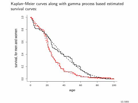
Kaplan–Meier curves along with gamma process based estimatedsurvival curves:

0 20 40 60 80 100

0.0

0.2

0.4

0.6

0.8

1.0

age

surv

ival,

for m

en a

nd w

omen

12/1001

2b: Application B: time to 2nd child after stillbirth

From the Norwegian Birth Registry: 451 married women whosefirst child died at birth (stillbirth). We read off T , the number ofmonths till the birth of the 2nd child. Model: 2nd child is bornwhen

Z (t) ∼ Gam(aM(t), 1) ≥ c ,

with M(t) = 1− exp[−{(t − t0)/θ}d ], and t0 = 9/12 (time inyears).

I find ML estimates (a, c , θ, d) from the 451 observations – with abit of trouble and care, since observations are on interval form,with ∆Nj ∼ Bin(Yj , hj), data for interval [`j , rj ]:

hj = Pr{T ∈ [`j , rj ] |T ≥ `j} = 1−G (c , aM(rj), 1)

G (c , aM(`j), 1)

for the different time intervals.

Model fits very well (via AIC, better than alternatives), also for theT =∞ individuals; cf. cure models.

13/1001

2 4 6 8 10 12 14

0.0

0.2

0.4

0.6

0.8

1.0

1.2

years since stillbirth

nonp

aram

etric

and

par

amet

ric in

tens

ity

Empirical and model-fitted hazard rates for the event of a 2ndchildbirth, after experiencing a first-born stillbirth, for a populationof 451 married Norwegian women.

14/1001

5 10 15

05

1015

2025

3035

years

Z pr

oces

ses

for 1

0 co

uple

s

Simulated Gamma processes for ten couples. The process needs tocross the level c = 17.45 (also plotted in the diagram), in order fora woman to have a 2nd child. With probabilityp = G (c , a, 1)

.= 0.097, there will never be a 2nd child.

15/1001

2c: Application C: regression for oropharynx survival data

Survival data (ti , δi , xi ,1, xi ,2, xi ,3, xi ,4) for n = 193 individuals, with

I x1: sex (1 male, 2 female);

I x2: condition (1-2-3-4, index of disability);

I x3: T-stage (1-2-3-4, size and infiltration of tumour);

I x4: N-stage (0-1-2-3, index of lymph node metastatis).

I take the gamma process time-to-hit model

ti = min{t ≥ 0: Zi (t) ≥ ci},

with Zi (t) ∼ Gam(aMi (t), 1), Mi (t) = 1− exp(−κi t),

ci = exp(β0 + β1xi ,1 + · · ·+ β4xi ,4),

κi = κ0 exp(γ(xi ,2 + xi ,3 + xi ,4)),

with at most 1 + 5 + 2 = 8 parameters. It does better thanAalen–Gjessing (2001) and other models (in terms of AIC and FICscores).

16/1001

0 1 2 3 4 5

0.0

0.2

0.4

0.6

0.8

1.0

years

surv

ival

, wom

en, l

ow, m

ediu

m, h

igh

risk

0 1 2 3 4 5

0.0

0.5

1.0

1.5

2.0

2.5

years

haza

rd, w

omen

, low

, med

ium

, hig

h ris

k

Estimated survival curves S(t) and hazard rate functions h(t) areplotted for three individuals, corresponding to high risk (c = 0.20),medium risk (c = 0.65) and low risk (c = 0.90). Hazards are notproportional (so Cox regression does worse).

17/1001

3a: Survival models via Gamma process jumps

Consider a Gamma process, Z (t) ∼ Gam(A(t), 1), withA(t) =

∫ t0 a(s) ds. There are jumps (mostly small, but some

bigger) over each time interval. Suppose an individual is alive aslong as all shocks are ≤ v . Need to find

S(t) = Pr{T ≥ t} = Pr{J(t) < v},

where J(t) is biggest jump over [0, t].

With Zm(t) =∑

j/m≤t Gm,j , and Gm,j ∼ Gam(a(j/m)(1/m), 1),we have Zm →d Z , and we can prove a Poisson limit:

Nm(t) =∑

j/m≤t

I (Gm,j > v)→d N(t) ∼ Pois(A(t)E1(v)),

with the exponential integral functionE1(v) =

∫∞v (1/u) exp(−u)du. So:

S(t) = Pr{N(t) = 0} = exp{−A(t)E1(v)}.

18/1001

We have ‘reinvented’ the Cox proportional hazards model, fromshocks of a Gamma process – the cumulative hazard rates (can)take the form

Hi (t) = A(t)E1(vi ) = A(t) exp(x ti β).

Variation I: Suppose individual is alive as long as 3 biggest shocksare below v . Then

S3(t) = Pr{N(t) ≤ 3} = exp{−B(t)}{1+B(t)+ 12B(t)2+ 1

6B(t)3},

with B(t) = A(t)E1(v). The hazard rate becomes

h3(t) = b(t)16B(t)3

1 + B(t) + 12B(t)2 + 1

6B(t)3= b(t)Q3(t),

with b(t) = a(t)E1(v) and Q3 growing from 0 to 1 over time.

Can fit each of S1,S2, S3, . . . to regression data and determine themixture proportions, or use AIC or FIC to select the best order.

19/1001

Variation II: Suppose some individuals ‘get used to shocks’ (andtolerate more) while others are ‘worn out by shocks’ (and tolerateless). Assume an individual is alive as long asGm,j ≤ v exp(γwj/m), in model formulation above. Then

Sm(t) =∏

j/m≤t

Pr{Gm,j ≤ v exp(γwj/m)}

=∏

j/m≤t

{1− a(j/m)(1/m)E1(v exp(γwj/m))}

→ exp{−∫ t

0a(s)E1(v exp(γws)) ds

}.

With survival regression data (ti , δi , xi ), we have an extended Coxmodel, with hazard rates

hi (t) = a(t)E1(vi exp(γwi s)), where E1(vi ) = exp(x ti β),

and wi is one of the covariates. Analysis for given data can providea confidence curve cc(γ).

20/1001

3b: Shocks and cumulative shocks, jointly

With a Z (t) ∼ Gam(A(t), 1), suppose an individual is alive as longas Z (t) < c and J(t) < v , where J(t) is biggest jump experiencedover [0, t].

This leads to amenable models if we can derive a formula for thesurvival, S(t) = Pr{Z (t) < c, J(t) < v}. Via Zm →d Z , withZm(t) =

∑j/m≤t Gm,j , we have Nm(t) =

∑j/m≤t I (Gm,j > v)

tending to a Poisson with A(t)E1(v), and we can prove

S(t) = Pr{Z (t) < c ,N(t) = 0}

=

∫ c

0Pr{N(t) = 0 | z}g(z ,A(t), 1) dz

=

∫ c

0Pr{J∗(t) < zv}g(z ,A(t), 1)dz ,

where J∗(t) is the biggest jump in a certain Dirichlet process D∗(·)over [0, t]. Can be done, via Hjort and Ongaro (2006) =⇒ fullinference.

21/1001

3c: Life is full of dangers

Suppose an invidual lives a life full of independent competingdangers, with cause j of event stemming from one of

Zj(t) ∼ Gam((1/m)b(j/m)M(t), 1) crossing threshold c(j/m).

Then with T = min(T1, . . . ,Tm), and m big,

S(t) = Pr{each Zj(t) < c( j

m

)} =

∏j≤m

G(c( j

m

),

1

mb( j

m

)M(t), 1

)=∏j≤m

{1− 1

mb( j

m

)M(t)E1

(c( j

m

))+ O(1/m2)

}→ exp

{−M(t)

∫ 1

0b(s)E1(c(s))ds

}.

This leads to a large class of plausible models, where specialsubclasses may be used for a set of given data.

22/1001

4: Extended logistic regression

Standard logistic regression:

pi = Pr(Yi = 1 | xi ) =exp(x ti β)

1 + exp(x ti β)

= G(log{1 + exp(x ti β)}, 1, 1

),

with G (·, a, 1) the c.d.f. of Gam(a, 1).

Extension:

pi = Pr(Yi = 1 | xi , zi ) = G(log{1 + exp(x ti β)}, ai , 1

),

where ai = a(zi ). Could have ai = exp(zti γ), and with somecovariates for the xi part and others for the zi part.

These models, where ‘event’ is seen as a gamma process reachinga threshold, are often better than plain logistic regressions, interms of AIC and FIC scores.

23/1001

Illustration: probability of child having birthweight ≤ 2.50 kg.With xi ,1, xi ,2 weight and age of mother,

pi =

{G (log{1 + exp(β0 + β1xi ,1 + β2xi ,2)}, 1 + δ, 1) if smoker

G (log{1 + exp(β0 + β1xi ,1 + β2xi ,2)}, 1− δ, 1) if nonsmoker.

40 60 80 100

0.0

0.1

0.2

0.3

0.4

0.5

0.6

mother's weight

prob

sm

all b

irthw

eigh

t

smoker

nonsmoker

24/1001

5a: Competing risks

Suppose each individual has two cumulative risk processes R1(t)and R2(t) in his or her rucksack. There is event (e.g. death) wheneither of these hit threshold c – of cause 1, if R1 is first; ofcause 2, if R2 is first.

First, new survival models emerge by working with new settings,with T = min(T1,T2), etc. An easy instance is

S(t) = Pr{T ≥ t} = G (c , a1M1(t), 1)G (c , a2M2(t), 1).

Second, can set up models and methods for competing risks.Simple setup:

Rj(t) ∼ Gam(ajMj(t), 1) for j = 1, 2,

with independence. Can then estimate all parameters from thistype of survival data,

(ti , xi , δi ), δi ∈ {0, 1, 2}.25/1001

Can also carry out the necessary characterisations andformalisation of likelihood components etc. for the case of

R1(t) = Z0(t) + Z1(t), R2(t) = Z0(t) + Z2(t),

with independent gamma processes Z0,Z1,Z2 (so full ML analysisis amenable). This opens up for dependent risk processes.

This machinery also leads to formulae for relevant statisticalparameters and functions, like

qj(t) = Pr{death of cause j , at t | death at time t}

for j = 1, 2. Theory for ML works well enough to supply alsoconfidence bands etc.

26/1001

5b: War of Roses (1455-1487) and Game of Thrones

We have 400 noblemen from the two universes. They die ofviolence or of natural causes.

I WoR: 126 dead men, 35% violence

I GoT: 274 dead men, 56 alive, 81% violence

We use two competing risk Gamma processes and time to hit:

Zn(t) ∼ Gam(antκn , 1) and Zv (t) ∼ Gam(av t

κv , 1).

Our model uses also L, the length of the wikipedia article:

αn = exp{βn,0 + βn,1I (GoT )},αv = exp{βv ,0 + βv ,1I (GoT ) + βv ,2L + βv ,3I (GoT )× L}.

Inference based on log-likelihood:

`(θ) =∑δi=0

log S(ti | θ) +∑δi=1

log f ∗1 (ti | θ) +∑δi=2

log f ∗2 (ti | θ).

27/1001

Fitted cumulative incidence functions compared withnonparametric estimators:

0.0

0.2

0.4

0.6

0.8

1.0

from WoR

age

0 25 50 75 100

natural fitted

violent fitted

natural np

violent np

0.0

0.2

0.4

0.6

0.8

1.0

from GoT

age

0 25 50 75 100

28/1001

The probability of dying of cause j given death at time t:qj(t) = f ∗j (t)/{f ∗1 (t) + · · ·+ f ∗k (t)}. Here:Pr{dies a violent death at t | dies at t}, in two universes.

0.0

0.2

0.4

0.6

0.8

1.0

age

P{v

iole

nt d

eath

at t

| de

ath

at ti

me

t}

0 25 50 75 100

WoR unimportant

WoR important

GoT unimportant

GoT important

29/1001

6: Frailtifying the Gamma process threshold model

My favourite Gamma process threshold model is: event takes placewhen Z (t) ≥ c , where Z (t) ∼ Gam(aM0(t), 1):

S(t | c) = Pr{T ≥ t | c} = G (c, aM0(t), 1).

Frailty: give c a distribution with distribution F0(c) = 1− S0(c).Then, observed in the population:

S(t) =

∫ ∞0

S(t | c) dF0(c)

=

∫ ∫I (x ≤ c)g(x , aM0(t), 1)dx dF0(c)

=

∫S0(x)

1

Γ(aM0(t))xaM0(t)−1 exp(−x) dx .

Frailty for thresholds translates to downweighting over time of thegamma density. (Can also frailtify over a.)

Special case: c ∼ Expo(γ) implies S(t) = exp{−bM0(t)}, withb = a log(1 + γ).

30/1001

7: Concluding remarks

1. Too often statisticians employ off-the-shelf models and methods.

2. My themes evolve around plausible processes =⇒ good models(and then good methods). Of course there is a literature on suchthemes (Aalen, Borgan, Gjessing, Lee, Whitmore, others), butthere is scope for more groundwork.

3. Many of the models coming out of plausible processes areamenable to ML and Bayes analyses etc.; some are semiparametricor nonparametric, with more work to be carried out.

4. Starting with classes of plausible processes one quickly has aplethora of candidate models – so scope for more work, sorting theVery Good Models from the not-as-successful models, e.g. usingmodel selection and model screeing methods (AIC, BIC, FIC).

5. Dynamics can be put into many of the models (covariateschanging over time; regime shifts).

31/1001

6. Models can be individualised, with applications for personalisedmedicine etc.

7. Two-stage models for events: (i) first Z1(t) ∼ Gam(M(t), 1) atwork, until threshold c1 at time T1; (ii) thenZ2(t) ∼ Gam(M∗(t), 1) sets in, with different M∗, and might hitc2. Links to cure models.

8. Gamma-Gamma process, to reflect more uncertainty (or randomeffects): Z |Z0 ∼ Gam(Z0, 1) and Z0 ∼ Gam(M, 1). Then

EZ (t) = M(t) and VarZ (t) = M(t) + M(t).

Can again work with time-to-threshold and time-to-jumpsize.

9. Excessive risk in some time periods:

dZi (t) = dZ0(t) + xi (t) dR(t) =

{dZ0(t) when normal,

dZ0(t) + dR(t) when danger.

With Gamma processes for Z0 and R, can make inference for theirparameters.

32/1001

(Some) references

Aalen, O.O., Borgan, Ø. and Gjessing, H. (2008). Survival and Event HistoryAnalysis: A Process Point of View. Springer.

Aalen, O.O. and Hjort, N.L. (2002). Frailty models that yield proportionalhazards. Statistics and Probability Letters.

Claeskens, G. and Hjort, N.L. (2008). Model Selection and Model Averaging.Cambridge University Press.

Cunen, C. and Hjort, N.L. (2018). Survival and event history models viagamma processes.

Gjessing, H., Aalen, O.O. and Hjort, N.L. (2003). Frailty models based on Levyprocesses. Advances in Applied Probability.

Green, P.J., Hjort, N.L., and Richardson, S. (2003). Highly StructuredStochastic Systems. Oxford University Press.

Hjort, N.L., Holmes, C., Muller, P. and Walker, S.G. (2010). BayesianNonparametrics. Cambridge University Press.

Hjort, N.L. and Ongaro, A. (2006). On the distribution of random Dirichletjumps. Metron.

Lee, M.-L.T. and Whitmore, G.A. (2006). Threshold regression for survivalanalysis: Satistical Science.

Schweder, T. and Hjort, N.L. (2016). Confidence, Likelihood, Probability.Cambridge University Press. 33/1001