Embed Size (px)
Citation preview
Superconductivity in
nanostructures: Andreev
billiards and Josephson
junction qubits
Marlies Goorden
ii
Superconductivity in
nanostructures: Andreev
billiards and Josephson
junction qubits
PROEFSCHRIFT
ter verkrijging vande graad van Doctor aan de Universiteit Leiden,
op gezag van de Rector Magnificus Dr. D. D. Breimer,hoogleraar in de faculteit der Wiskunde en
Natuurwetenschappen en die der Geneeskunde,volgens besluit van het College voor Promoties
te verdedigen op 15 september 2005te klokke 15.15 uur
door
Marlies Cornelia Goorden
geboren te Sittard op 26 december 1976
Promotiecommissie:
Promotor: Prof. dr. C. W. J. BeenakkerReferent: Prof. dr. ir. W. van SaarloosOverige leden: Prof. dr. M. Grifoni
Prof. dr. Ph. JacquodProf. dr. P. H. KesProf. dr. ir. J. E. MooijDr. P. G. Silvestrov
Het onderzoek beschreven in dit proefschrift is onderdeel van het weten-schappelijke programma van de Stichting voor Fundamenteel Onderzoekder Materie (FOM) en de Nederlandse Organisatie voor WetenschappelijkOnderzoek (NWO).The research described in this thesis has been carried out as part of thescientific programme of the Foundation for Fundamental Research on Mat-ter (FOM) and the Netherlands Organisation for Scientific Research (NWO).
Alexander V. Andreev

vi
Contents
1 Introduction 11.1 Andreev reflection . . . . . . . . . . . . . . . . . . . . . . . . . . . 2
1.1.1 Reflection mechanism . . . . . . . . . . . . . . . . . . . . 21.1.2 Excitation gap . . . . . . . . . . . . . . . . . . . . . . . . . 51.1.3 Josephson effect . . . . . . . . . . . . . . . . . . . . . . . . 6
1.2 Andreev billiard . . . . . . . . . . . . . . . . . . . . . . . . . . . . 61.2.1 Chaotic vs. integrable billiard . . . . . . . . . . . . . . . . 71.2.2 Quantum-to-classical crossover . . . . . . . . . . . . . . 9
1.3 Josephson junction qubit . . . . . . . . . . . . . . . . . . . . . . 121.4 This thesis . . . . . . . . . . . . . . . . . . . . . . . . . . . . . . . . 16
2 Adiabatic quantization of an Andreev billiard 272.A Effective RMT . . . . . . . . . . . . . . . . . . . . . . . . . . . . . . 36
3 Quasiclassical fluctuations of the superconductor proximity gapin a chaotic system 45
4 Quantum-to-classical crossover for Andreev billiards in a mag-netic field 574.1 Introduction . . . . . . . . . . . . . . . . . . . . . . . . . . . . . . . 574.2 Adiabatic quantization . . . . . . . . . . . . . . . . . . . . . . . . 58
4.2.1 Classical mechanics . . . . . . . . . . . . . . . . . . . . . . 584.2.2 Adiabatic invariant . . . . . . . . . . . . . . . . . . . . . . 604.2.3 Quantization . . . . . . . . . . . . . . . . . . . . . . . . . . 634.2.4 Lowest adiabatic level . . . . . . . . . . . . . . . . . . . . 644.2.5 Density of states . . . . . . . . . . . . . . . . . . . . . . . . 66
4.3 Effective random-matrix theory . . . . . . . . . . . . . . . . . . . 674.3.1 Effective cavity . . . . . . . . . . . . . . . . . . . . . . . . . 67
vii
4.3.2 Density of states . . . . . . . . . . . . . . . . . . . . . . . . 694.4 Comparison with quantum mechanical model . . . . . . . . . . 734.5 Conclusion . . . . . . . . . . . . . . . . . . . . . . . . . . . . . . . 764.A Andreev kicked rotator in a magnetic field . . . . . . . . . . . . 78
5 Noiseless scattering states in a chaotic cavity 85
6 Spectroscopy of a driven solid-state qubit coupled to a structuredenvironment 976.1 Introduction . . . . . . . . . . . . . . . . . . . . . . . . . . . . . . . 976.2 The driven qubit coupled to a macroscopic detector . . . . . 1006.3 Weak coupling: Floquet-Born-Markov master equation . . . . 103
6.3.1 Floquet formalism and Floquet-Born-Markovian mas-ter equation . . . . . . . . . . . . . . . . . . . . . . . . . . . 103
6.3.2 Van Vleck perturbation theory . . . . . . . . . . . . . . . 1056.3.3 Line shape of the resonant peak/dip . . . . . . . . . . . 1096.3.4 Example: The first blue sideband . . . . . . . . . . . . . 1096.3.5 Results and discussion . . . . . . . . . . . . . . . . . . . . 113
6.4 Strong coupling: NIBA . . . . . . . . . . . . . . . . . . . . . . . . 1146.5 Limit Ωp ν . . . . . . . . . . . . . . . . . . . . . . . . . . . . . 1176.6 Conclusions . . . . . . . . . . . . . . . . . . . . . . . . . . . . . . . 1206.A Symmetry properties for the dissipative rates for the first
blue sideband . . . . . . . . . . . . . . . . . . . . . . . . . . . . . . 1216.B Coefficients for the kernels k±0 (0) . . . . . . . . . . . . . . . . . 123
Samenvatting 127
List of publications 131
Curriculum Vitæ 133
Dankwoord 135
viii
Chapter 1
Introduction
Fundamental research on superconductivity can be broadly divided intotwo classes, each with its own motivation. The first class of researchstudies novel mechanisms of electron pairing, that might persist at highertemperatures than the conventional phonon-mediated pairing. The secondclass studies novel effects that occur when conventionally paired electronsare confined to structures of sub-micrometer dimensions (so-called nanos-tructures). The motivation here is not the search for higher transition tem-peratures, but the integration of superconducting elements in computercircuits. The research described in this thesis falls in the second class, thestudy of superconductivity in nanostructures.
Two types of nanostructures have been investigated, Andreev billiardsand Josephson junction qubits. An Andreev billiard is an impurity-free re-gion in a two-dimensional electron gas (a so-called quantum dot), cou-pled to a superconducting electrode via a point contact. The fundamentalquestion that we have answered is how the excitation gap of the electrongas, caused by Andreev reflection at the superconductor, depends on theEhrenfest time. This time scale governs the crossover from classical toquantum chaos in quantum dots.
A Josephson junction qubit is a superconducting ring in which the di-rection of the current is a quantum mechanical superposition of clock-wise and counter-clockwise. Such a device is one of the possible buildingblocks of a quantum computer. To describe existing experiments we havedeveloped a quantitative theory that takes into account both the time-dependent external magnetic field used to control the qubit and its cou-
2 Chapter 1. Introduction
I S
e
e
e
h
NN
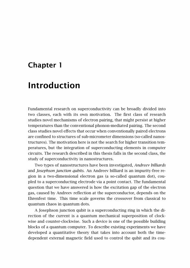
Figure 1.1: Normal reflection (left) vs. Andreev reflection. Upon normalreflection at the interface between an insulator (I) and a normal metal (N)only the component of the velocity normal to the interface changes signand the charge is conserved. In the case of Andreev reflection at a normal-metal-superconductor (NS) interface all three components of the velocitychange sign and the negatively charged electron is converted into a posi-tively charged hole.
pling to a quantum measurement device.
In this introductory chapter we present some background material forthe topics studied in the thesis.
1.1 Andreev reflection
The anomalous reflection at the interface between a normal metal (N) anda superconductor (S), discovered by Andreev in 1964 [1], plays a centralrole in this thesis. Andreev reflection, as this process is now called, ex-plains the opening of an excitation gap in the billiard geometry and itexplains the flow of a non-decaying current in the ring geometry (the so-called Josephson effect).
1.1.1 Reflection mechanism
The process of Andreev reflection is illustrated in Fig. 1.1. When a nega-tively charged electron in the normal metal hits the interface with the su-
1.1 Andreev reflection 3
perconductor (NS interface) it is converted into a positively charged hole.The hole retraces the path of the electron, so its velocity is reversed (so-called retroreflection). Because the hole has a negative mass, the totalmomentum is conserved. The charge difference of 2e between electronand hole is compensated by the creation of a Cooper pair with charge 2ein the superconductor. In contrast, specular reflection between a normalmetal and an insulator (also shown in Fig. 1.1) conserves the charge, butnot the momentum.
The velocity is only exactly reversed when electron and hole are bothat the Fermi level. When the electron has an excitation energy E abovethe Fermi energy EF it is converted into a hole with energy −E, and as aconsequence there is a slight mismatch between their velocities: while themagnitude of the velocity parallel to the superconductor is conserved, theperpendicular velocity differs in magnitude by
√4E/m.
A quantum mechanical description of Andreev reflection starts from aSchrodinger equation for the electron and hole components u(r) and v(r)of the wave function, coupled by the pair potential ∆(r). This so-calledBogoliubov-de Gennes (BdG) equation is given by [2]
(H0 ∆(r)∆∗(r) −H∗0
)(uv
)= E
(uv
). (1.1)
It contains the Hamiltonian H0 = [p+ eA(r)]2 /2m+ V(r)− EF of a singleelectron moving with momentum p in an electrostatic potential V and vec-tor potential A. The pair potential ∆(r) ≡ 0 in the normal region while itrecovers the bulk value ∆0eiφ of the superconductor at some distance lcaway from the interface. For the geometries considered in this thesis thestep function
∆(r) =
0 if r ∈ N∆0eiφ if r ∈ S (1.2)
is sufficiently accurate (because lc is much smaller than the superconduct-ing coherence length vF/∆0). The excitation spectrum consists of thesolution of Eq. (1.1) with E ≥ 0.
Referring to the geometry of Fig. 1.2 the eigenfunctions of the BdG
4 Chapter 1. Introduction
N S
x
y
0e
0
x0
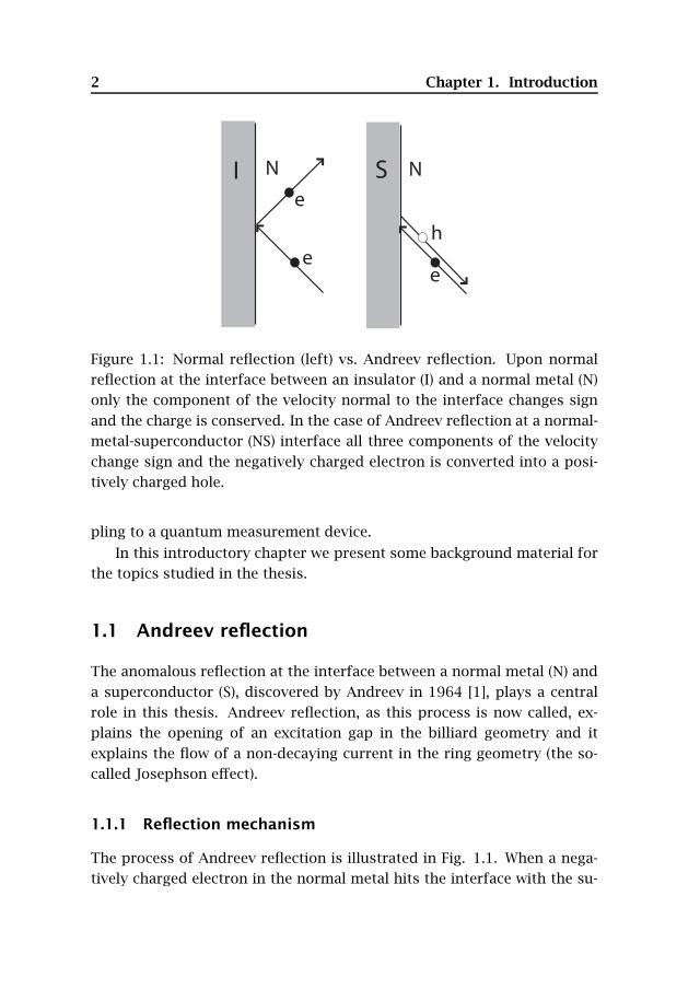
Figure 1.2: Geometry of an NS junction (bottom) and plot of the absolutevalue of the pair potential (top), in the step function model of Eq. (1.2).
equation in the normal metal can be written as
ψ±n,e =(
10
)1√kenΦn(y, z) exp(±ikenx), (1.3)
ψ±n,h =(
01
)1√khnΦn(y, z) exp(±ikhnx), (1.4)
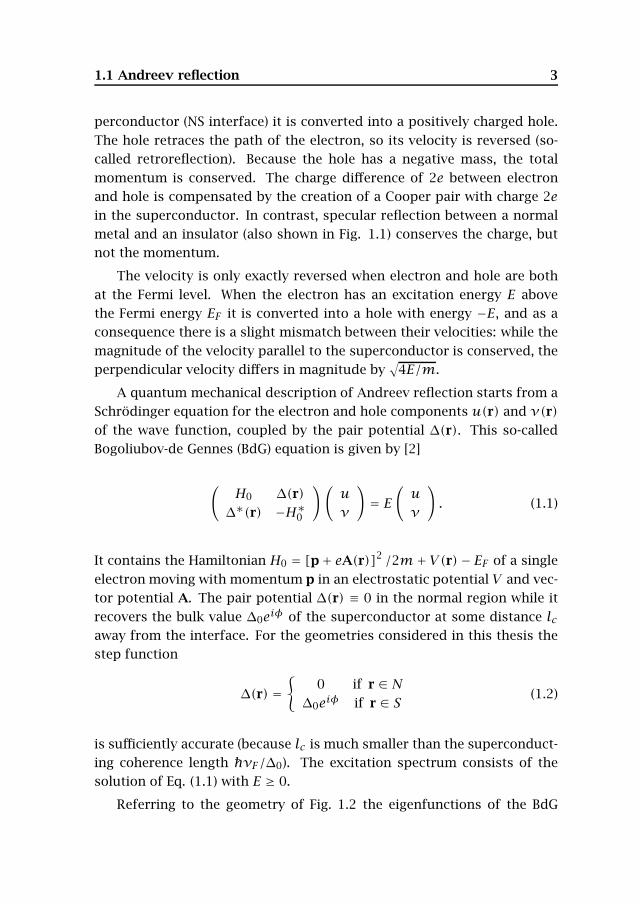
ke,hn = (2m/2)1/2(EF − En +σe,hE)1/2, (1.5)
with σe = 1 and σh = −1. The discrete wave numbers ke,hn originate fromthe confinement in y and z direction, with the index n labeling the dif-ferent modes. The n-th mode has transverse wave function Φn(y, z) andthreshold energy En. The wavefunctions are normalized to carry the sameamount of quasiparticle current if the functions Φn(y, z) are normalizedto unity.
In the superconductor the solutions of the BdG equation give decay-ing eigenfunctions for E < ∆0, indicating that there are no propagatingmodes in the superconductor for these energies. Matching the eigenfunc-tions in the normal metal and superconductor at the NS boundary de-termines the scattering at the superconductor. For ∆0 EF and in theabsence of a barrier at the NS interface there is no normal reflection, only
1.1 Andreev reflection 5
NS
x
y S he
0e
0
x
2
0e 1
0
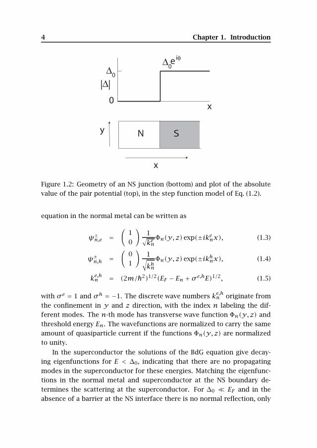
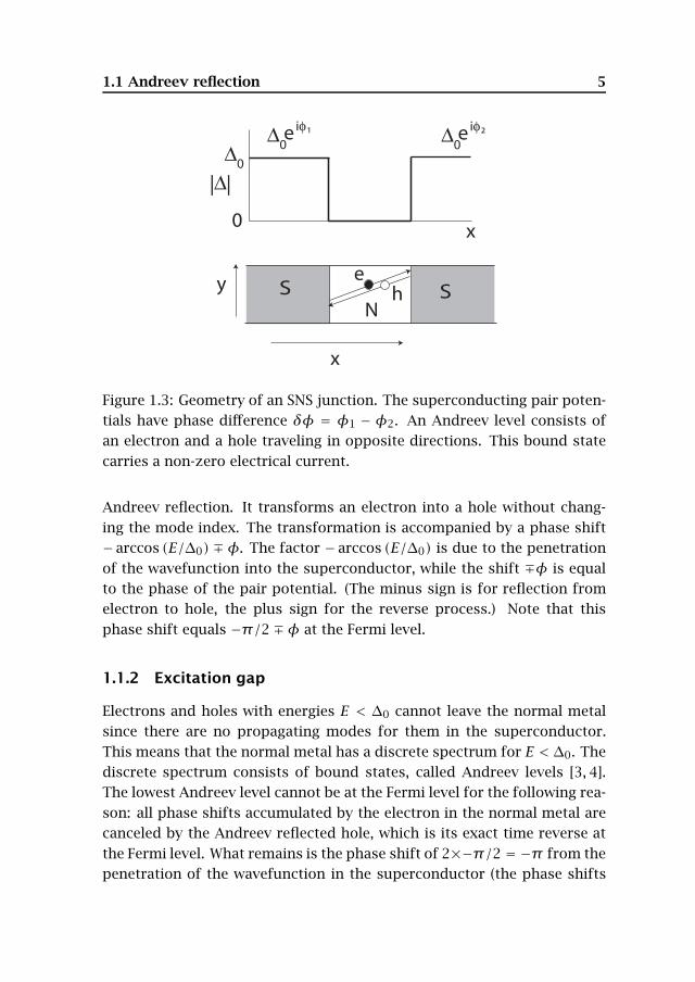
Figure 1.3: Geometry of an SNS junction. The superconducting pair poten-tials have phase difference δφ = φ1 − φ2. An Andreev level consists ofan electron and a hole traveling in opposite directions. This bound statecarries a non-zero electrical current.
Andreev reflection. It transforms an electron into a hole without chang-ing the mode index. The transformation is accompanied by a phase shift−arccos (E/∆0)∓φ. The factor − arccos (E/∆0) is due to the penetrationof the wavefunction into the superconductor, while the shift ∓φ is equalto the phase of the pair potential. (The minus sign is for reflection fromelectron to hole, the plus sign for the reverse process.) Note that thisphase shift equals −π/2 ∓φ at the Fermi level.
1.1.2 Excitation gap
Electrons and holes with energies E < ∆0 cannot leave the normal metalsince there are no propagating modes for them in the superconductor.This means that the normal metal has a discrete spectrum for E < ∆0. Thediscrete spectrum consists of bound states, called Andreev levels [3, 4].The lowest Andreev level cannot be at the Fermi level for the following rea-son: all phase shifts accumulated by the electron in the normal metal arecanceled by the Andreev reflected hole, which is its exact time reverse atthe Fermi level. What remains is the phase shift of 2×−π/2 = −π from thepenetration of the wavefunction in the superconductor (the phase shifts
6 Chapter 1. Introduction
∓φ cancel as well). So electron and hole interfere destructively at theFermi level and the lowest excited state must be separated by some en-ergy Egap from EF . The calculation of Egap is the problem of the Andreevbilliard, introduced in Sec. 1.2.
1.1.3 Josephson effect
Now consider an SNS junction having two NS interfaces with a phase dif-ference δφ = φ1 − φ2 of the pair potentials (Fig. 1.3). An Andreev levelcorresponds to an electron moving towards one superconductor, whereit is converted into a hole which goes to the other superconductor to beretroreflected again as an electron.
The excitation gap Egap closes when δφ = π , because then the electronand hole at the Fermi level interfere constructively rather than destruc-tively (as they do when δφ = 0). Not only Egap depends on δφ, but thetotal energy U of the SNS junction is δφ-dependent. The current I whichflows from one superconductor to the other is related to U(δφ) by
I = 2edUdδφ
. (1.6)
This current is present in the SNS junction in equilibrium, so it cannot de-cay. Since I depends periodically on δφ ∈ (0,2π), it reaches a maximumfor some δφ at a value called the critical current Ic .
The original discovery by Josephson of this effect [5] was done for thecase that the normal metal is a tunnel junction (relevant for our Josephsonjunction qubit). Then U = EJ(1 − cosδφ), where EJ = π∆0G/4e2 [6] isdetermined by the tunnel conductance G. The current-phase relationshipbecomes
I = Ic sinδφ, Ic = 2eEJ (1.7)
The connection between the Josephson effect and Andreev reflection inballistic SNS junctions was made by Kulik [7].
1.2 Andreev billiard
An electro-micrograph of an Andreev billiard is shown in Fig. 1.4. A con-fined region in a two-dimensional electron gas is created by means of gate
1.2 Andreev billiard 7
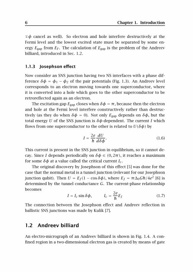
Figure 1.4: Quantum dot (central square of dimensions 500 nm× 500 nm)fabricated in a high-mobility InAs/AlSb heterostructure and contacted byfour superconducting Nb electrodes. Device made by A. T. Filip, GroningenUniversity (unpublished figure).
electrodes. These electrodes provide insulating barriers, at which normalspecular reflection occurs. Four superconducting electrodes introduce An-dreev reflection (retroreflection).
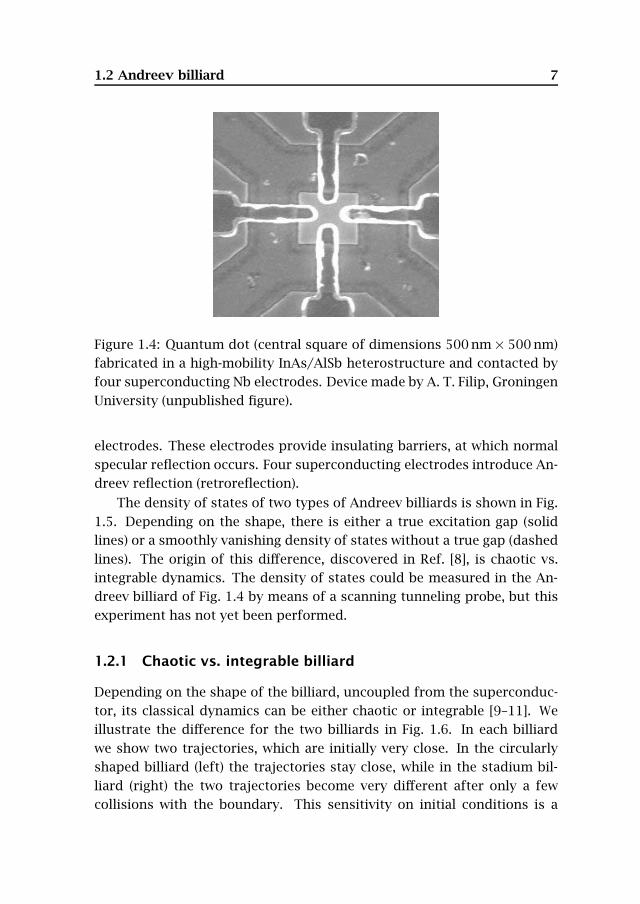
The density of states of two types of Andreev billiards is shown in Fig.1.5. Depending on the shape, there is either a true excitation gap (solidlines) or a smoothly vanishing density of states without a true gap (dashedlines). The origin of this difference, discovered in Ref. [8], is chaotic vs.integrable dynamics. The density of states could be measured in the An-dreev billiard of Fig. 1.4 by means of a scanning tunneling probe, but thisexperiment has not yet been performed.
1.2.1 Chaotic vs. integrable billiard
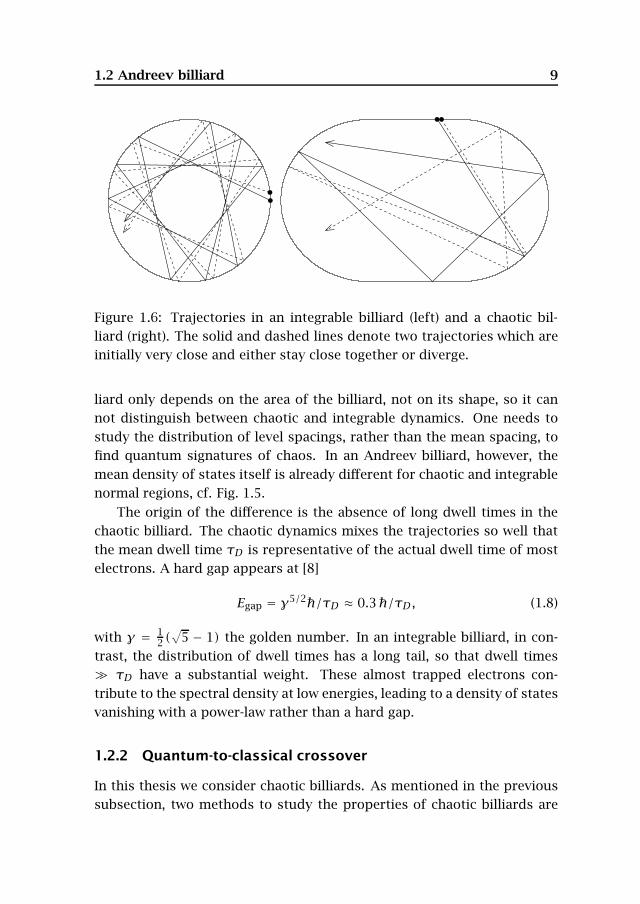
Depending on the shape of the billiard, uncoupled from the superconduc-tor, its classical dynamics can be either chaotic or integrable [9–11]. Weillustrate the difference for the two billiards in Fig. 1.6. In each billiardwe show two trajectories, which are initially very close. In the circularlyshaped billiard (left) the trajectories stay close, while in the stadium bil-liard (right) the two trajectories become very different after only a fewcollisions with the boundary. This sensitivity on initial conditions is a
8 Chapter 1. Introduction
Figure 1.5: Mean density of states for a chaotic Andreev billiard (top inset)and an integrable Andreev billiard (bottom inset). The histograms are theexact quantum mechanical solution, obtained numerically. The smoothcurves are the analytical predictions. From Ref. [15].
characteristic of chaotic dynamics: two trajectories which are initially ata distance δ(0), have diverged to δ(t) = δ(0) exp (λt) after a time t. TheLyapunov exponent λ determines the strength of the divergence.
Quantum mechanical properties of chaotic systems are the subject ofthe field of quantum chaos [12–14]. A billiard is one of the most sim-ple systems to study in this context. The properties of normal billiards(normal meaning that there is no superconducting segment in the bound-ary) have been studied extensively in the past. A universal description ofchaotic systems is provided by random-matrix theory (RMT) [16], while adirect way of connecting classical and quantum mechanics is provided byperiodic orbit theory [10]. The mean density of states of a normal bil-
1.2 Andreev billiard 9
Figure 1.6: Trajectories in an integrable billiard (left) and a chaotic bil-liard (right). The solid and dashed lines denote two trajectories which areinitially very close and either stay close together or diverge.
liard only depends on the area of the billiard, not on its shape, so it cannot distinguish between chaotic and integrable dynamics. One needs tostudy the distribution of level spacings, rather than the mean spacing, tofind quantum signatures of chaos. In an Andreev billiard, however, themean density of states itself is already different for chaotic and integrablenormal regions, cf. Fig. 1.5.
The origin of the difference is the absence of long dwell times in thechaotic billiard. The chaotic dynamics mixes the trajectories so well thatthe mean dwell time τD is representative of the actual dwell time of mostelectrons. A hard gap appears at [8]
Egap = γ5/2/τD ≈ 0.3/τD, (1.8)
with γ = 12(√
5 − 1) the golden number. In an integrable billiard, in con-trast, the distribution of dwell times has a long tail, so that dwell times τD have a substantial weight. These almost trapped electrons con-tribute to the spectral density at low energies, leading to a density of statesvanishing with a power-law rather than a hard gap.
1.2.2 Quantum-to-classical crossover
In this thesis we consider chaotic billiards. As mentioned in the previoussubsection, two methods to study the properties of chaotic billiards are
10 Chapter 1. Introduction
S N
e
eh
h
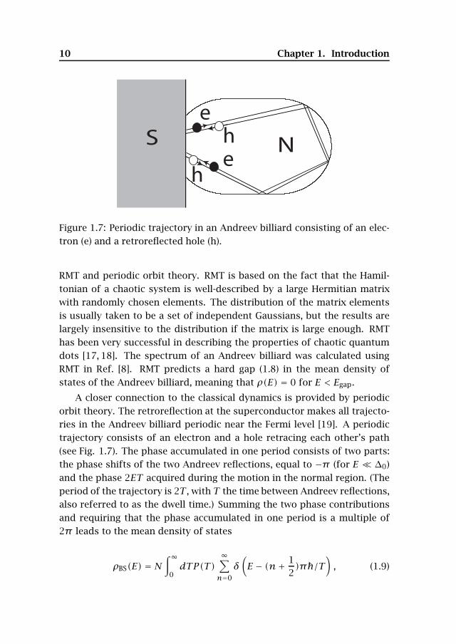
Figure 1.7: Periodic trajectory in an Andreev billiard consisting of an elec-tron (e) and a retroreflected hole (h).
RMT and periodic orbit theory. RMT is based on the fact that the Hamil-tonian of a chaotic system is well-described by a large Hermitian matrixwith randomly chosen elements. The distribution of the matrix elementsis usually taken to be a set of independent Gaussians, but the results arelargely insensitive to the distribution if the matrix is large enough. RMThas been very successful in describing the properties of chaotic quantumdots [17, 18]. The spectrum of an Andreev billiard was calculated usingRMT in Ref. [8]. RMT predicts a hard gap (1.8) in the mean density ofstates of the Andreev billiard, meaning that ρ(E) = 0 for E < Egap.
A closer connection to the classical dynamics is provided by periodicorbit theory. The retroreflection at the superconductor makes all trajecto-ries in the Andreev billiard periodic near the Fermi level [19]. A periodictrajectory consists of an electron and a hole retracing each other’s path(see Fig. 1.7). The phase accumulated in one period consists of two parts:the phase shifts of the two Andreev reflections, equal to −π (for E ∆0)and the phase 2ET acquired during the motion in the normal region. (Theperiod of the trajectory is 2T , with T the time between Andreev reflections,also referred to as the dwell time.) Summing the two phase contributionsand requiring that the phase accumulated in one period is a multiple of2π leads to the mean density of states
ρBS(E) = N∫∞
0dTP(T)
∞∑n=0
δ(E − (n+ 1
2)π/T
), (1.9)
1.2 Andreev billiard 11
where P(T) is the classical dwell time distribution and N is the number ofmodes in the point contact connecting the normal region with the super-conductor. This result is the Bohr-Sommerfeld approximation of Ref. [8].
A chaotic billiard has an exponential dwell time distribution P(T) =exp (−T/τD)τ−1
D , with τD = 2π/Nδ the mean dwell time and δ the meanlevel spacing of the isolated billiard. Substitution of this distribution intoEq. (1.9) results in the density of states [20]
ρBS(E) = 2δ(πET/E)2 cosh(πET/E)
sinh2(πET /E), (1.10)
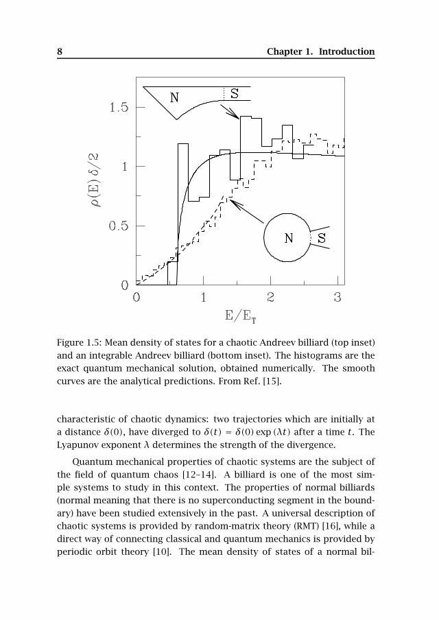
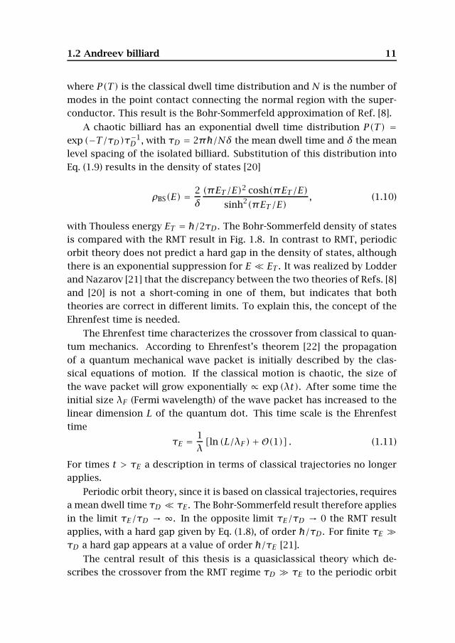
with Thouless energy ET = /2τD . The Bohr-Sommerfeld density of statesis compared with the RMT result in Fig. 1.8. In contrast to RMT, periodicorbit theory does not predict a hard gap in the density of states, althoughthere is an exponential suppression for E ET . It was realized by Lodderand Nazarov [21] that the discrepancy between the two theories of Refs. [8]and [20] is not a short-coming in one of them, but indicates that boththeories are correct in different limits. To explain this, the concept of theEhrenfest time is needed.
The Ehrenfest time characterizes the crossover from classical to quan-tum mechanics. According to Ehrenfest’s theorem [22] the propagationof a quantum mechanical wave packet is initially described by the clas-sical equations of motion. If the classical motion is chaotic, the size ofthe wave packet will grow exponentially ∝ exp (λt). After some time theinitial size λF (Fermi wavelength) of the wave packet has increased to thelinear dimension L of the quantum dot. This time scale is the Ehrenfesttime
τE = 1λ[ln (L/λF)+O(1)] . (1.11)
For times t > τE a description in terms of classical trajectories no longerapplies.
Periodic orbit theory, since it is based on classical trajectories, requiresa mean dwell time τD τE . The Bohr-Sommerfeld result therefore appliesin the limit τE/τD → ∞. In the opposite limit τE/τD → 0 the RMT resultapplies, with a hard gap given by Eq. (1.8), of order /τD . For finite τE τD a hard gap appears at a value of order /τE [21].
The central result of this thesis is a quasiclassical theory which de-scribes the crossover from the RMT regime τD τE to the periodic orbit
12 Chapter 1. Introduction
0
0.5
1
0 0.5 1 1.5
(E
)2/
E / ET
BS
RMT
Figure 1.8: Comparison of the mean density of states ρ(E) of a chaoticAndreev billiard, as it is predicted by random-matrix theory (RMT) and byperiodic orbit theory (or Bohr-Sommerfeld quantization, labeled BS). WhileRMT (valid for τE τD) predicts a hard gap, Bohr-Sommerfeld quantiza-tion (valid in the opposite limit τE τD) gives an exponential suppressionat low energies, without a hard gap. From Ref. [23].
regime τD τE . Our approach is very simple in principle: for short classi-cal trajectories T < τE we use periodic orbit theory while for long classicaltrajectories T > τE we use RMT with effective τE -dependent parameters(effective RMT). Since an experimental test is still lacking, we compare ourtheory with quantum mechanical simulations. The numerical model weuse is the Andreev kicked rotator [24], which provides a stroboscopic de-scription of an Andreev billiard. The model is very efficient and allows oneto go to large enough system sizes to reach the regime τE τD .
1.3 Josephson junction qubit
Superconducting circuits with Josephson junctions can be designed tohave states that carry circulating currents of opposite sign. This meansthat quantum mechanically the system can be in a macroscopic superpo-sition of clockwise and counter-clockwise circulating currents [25]. Theword “macroscopic” is used because a macroscopic number of Cooper
1.3 Josephson junction qubit 13
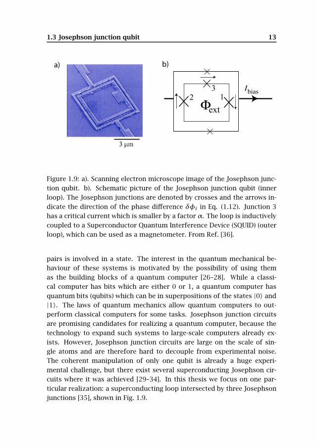
Figure 1.9: a). Scanning electron microscope image of the Josephson junc-tion qubit. b). Schematic picture of the Josephson junction qubit (innerloop). The Josephson junctions are denoted by crosses and the arrows in-dicate the direction of the phase difference δφi in Eq. (1.12). Junction 3has a critical current which is smaller by a factor α. The loop is inductivelycoupled to a Superconductor Quantum Interference Device (SQUID) (outerloop), which can be used as a magnetometer. From Ref. [36].
pairs is involved in a state. The interest in the quantum mechanical be-haviour of these systems is motivated by the possibility of using themas the building blocks of a quantum computer [26–28]. While a classi-cal computer has bits which are either 0 or 1, a quantum computer hasquantum bits (qubits) which can be in superpositions of the states |0〉 and|1〉. The laws of quantum mechanics allow quantum computers to out-perform classical computers for some tasks. Josephson junction circuitsare promising candidates for realizing a quantum computer, because thetechnology to expand such systems to large-scale computers already ex-ists. However, Josephson junction circuits are large on the scale of sin-gle atoms and are therefore hard to decouple from experimental noise.The coherent manipulation of only one qubit is already a huge experi-mental challenge, but there exist several superconducting Josephson cir-cuits where it was achieved [29–34]. In this thesis we focus on one par-ticular realization: a superconducting loop intersected by three Josephsonjunctions [35], shown in Fig. 1.9.
14 Chapter 1. Introduction
a)
Φ <0.5Φext 0 Φ =0.5Φext 0
1
-1
0
I/I
max
0.5 Φ /Φext 0
b)
0
Ei
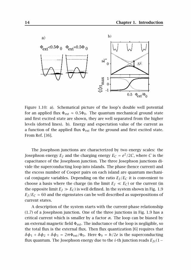
Figure 1.10: a). Schematical picture of the loop’s double well potentialfor an applied flux Φext ≈ 0.5Φ0. The quantum mechanical ground stateand first excited state are shown, they are well separated from the higherlevels (dotted lines). b). Energy and expectation value of the current asa function of the applied flux Φext for the ground and first excited state.From Ref. [36].
The Josephson junctions are characterized by two energy scales: theJosephson energy EJ and the charging energy EC = e2/2C, where C is thecapacitance of the Josephson junction. The three Josephson junctions di-vide the superconducting loop into islands. The phase (hence current) andthe excess number of Cooper pairs on each island are quantum mechani-cal conjugate variables. Depending on the ratio EJ/EC it is convenient tochoose a basis where the charge (in the limit EJ EC ) or the current (inthe opposite limit EJ EC ) is well defined. In the system shown in Fig. 1.9EJ/EC 60 and the eigenstates can be well described as superpositions ofcurrent states.
A description of the system starts with the current-phase relationship(1.7) of a Josephson junction. One of the three junctions in Fig. 1.9 has acritical current which is smaller by a factor α. The loop can be biased byan external magnetic field Φext. The inductance of the loop is negligible, sothe total flux is the external flux. Then flux quantization [6] requires thatδφ1 + δφ2 + δφ3 = 2πΦext/Φ0. Here Φ0 = h/2e is the superconductingflux quantum. The Josephson energy due to the i-th junction reads EJi(1−
1.3 Josephson junction qubit 15
cosδφi). Combining this with the flux quantization, the total Josephsonenergy U is given by
U = EJ [2+α− cosδφ1 − cosδφ2 −α cos(2πΦext/Φ0 − δφ1 − δφ2)] .(1.12)
It is a function of two phases. For a range of magnetic fields, this clas-sical potential has two stable solutions: one corresponding to a currentflowing clockwise, the other to a current flowing counter-clockwise. Themagnitude Imax of both currents is equal and it is very close to the crit-ical current of the weakest junction. By adding the charging energy andconsidering the circuit quantum mechanically, the quantum mechanicaleigenstates can be determined [37]. For suitably chosen parameters (α 0.6 − 0.8, EJ/EC 60), the system can be well-described as a two-statequantum system, in the vicinity of Φext = 1
2Φ0. The two eigenstates corre-spond to superpositions of states with opposite currents.
This is illustrated in Fig. 1.10. The classical double-well potential isshown, with the wells corresponding to currents of opposite sign. Quan-tum mechanically the qubit has two low-energy eigenstates (black andgray) which are well-separated from the higher lying levels. For Φext =12Φ0 the energies of the two wells are equal and the quantum mechanicalstates are symmetric and anti-symmetric superpositions of the two cur-rent states. For Φext below or above 1
2Φ0 the quantum states are morelocalized in one of the two wells. In Fig. 1.10 the expectation value of thecurrent as a function of Φext is also shown, both for the ground and ex-cited state. The current produces a magnetic field, which can be detectedby a Superconducting Quantum Interference Device (SQUID), shown in Fig.1.9.
The Hamiltonian of the Josephson junction qubit can be written in theform of a spin 1/2 particle,
HQ = −W2 σx − F2 σz , (1.13)
where σi are Pauli matrices. The tunnel splitting W depends on the de-tails of the junctions and it cannot be manipulated during the experiment.The static energy bias F = 2Imax
(Φext − 1
2Φ0
)can be tuned by changing
the applied flux.The state of the qubit can be controlled by applying a time-dependent
magnetic field in the GHz range, introducing a time dependence in the
16 Chapter 1. Introduction
energy bias F . If the control field is resonant with the energy splitting ofthe ground and excited state, coherent oscillations between the two levelsoccur. These Rabi oscillations have been measured [33]. For a quantitativedescription of the experiment one has to take into account the presence ofthe quantum measurement device (the SQUID) and the fact that the systemis periodically driven. In a recent experiment it has been found that thepresence of the SQUID introduces extra resonances [38]. The last chapterof the thesis is devoted to a quantitative description of this experiment.
1.4 This thesis
Chapter 2: Adiabatic quantization of an Andreev billiard
Periodic orbit theory gives a reliable description of the energy levels andwave functions of a normal billiard, provided it is large compared to theelectron wave length. In this chapter we apply this quasiclassical approachto Andreev billiards.
We start by studying the classical dynamics of electrons and holes.For finite excitation energies an Andreev reflected hole does not exactlyretrace the path of the electron. The slow drift has an adiabatic invariant:the time T between Andreev reflections. The adiabatically invariant torusin phase space can be quantized, resulting in a ladder of Andreev levels.The adiabatic quantization breaks down for T > τE . For this part of phasespace we propose an effective RMT. The result is a quantitative predictionfor the dependence of the excitation gap on the Ehrenfest time τE and thedwell time τD, which agrees well with computer simulations [24].
Chapter 3: Quasiclassical fluctuations of the superconductor prox-imity gap in a chaotic system
Mesoscopic systems have universal sample-to-sample fluctuations. Uni-versal means that their size does not depend on the exact miscroscopicproperties of the system. A well-known example are the universal conduc-tance fluctuations, which occur both in disordered and chaotic ballisticsystems. They can be described by RMT.
In this chapter we focus on the sample-to-sample fluctuations in the ex-citation gap of the Andreev billiard. In Ref. [39] the universal distribution
1.4 This thesis 17
function of the gap is calculated using RMT. It has a standard deviation
δERMT0 = 1.09ET/N2/3. (1.14)
For τE τD RMT breaks down. Since the Ehrenfest time scales only log-arithmically with L/λF , a numerical investigation of the regime τE τDdemands a very effective numerical model. This is provided by the An-dreev kicked rotator [24].
We use the Andreev kicked rotator to investigate the effect of theEhrenfest time on the gap fluctuations. We find that in the quasiclass-cial regime, the amplitude of the fluctuations is much larger than the RMTvalue (1.14). The effective RMT of chapter 2 gives a good description ofthe fluctuations.
Chapter 4: Quantum-to-classical crossover of Andreev billiardsin a magnetic field
We continue our development of the periodic orbit theory of Andreev bil-liards by studying the effect of a perpendicular magnetic field. RMT pre-dicts that the excitation gap of the Andreev billiard will be reduced with in-creasing field strength and that it will close at a critical magnetic field [15]
B0 eL2
√L
vFτD. (1.15)
We extend the quasiclassical theory of chapter 2 to include a time-reversal-symmetry breaking magnetic field. The critical magnetic field isreduced with increasing τE . We compare our quasiclassical expressionswith numerical results from the Andreev kicked rotator.
Chapter 5: Noiseless scattering states in a chaotic cavity
In this chapter we apply the effective RMT, developed in chapter 2 forthe Andreev billiard to a different system: a quantum dot which is notattached to a superconductor, but to two electron reservoirs. Throughsuch a system a current I(t) can flow. Due to the discreteness of chargethe current will fluctuate around its time averaged value I, even for zerotemperature. These fluctuations are known as shot noise. The shot noise

18 Chapter 1. Introduction
0.05
0.1
0.15
0.2
0.25
0.3
F
K = 7
0.05
0.1
0.15
0.2
0.25
0.3
102 103 104 105
F
M
K = 21τD = 5
1030
0.05
0.1
0.15
0.2
0.25
0.3
F
K = 14
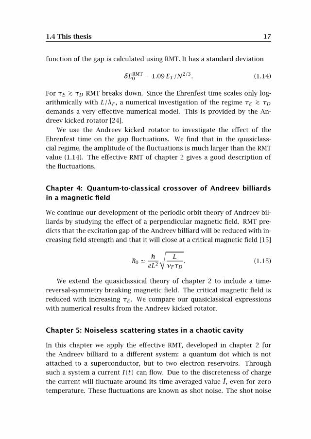
Figure 1.11: Dependence of the Fano factor F on the dimensionality ofHilbert space M L/λF , at fixed dwell time τD = (M/2N) × τ0. Thedata points are from a quantum mechanical simulation of the open kickedrotator with kicking strength K, Lyapunov exponent λ ln (K/2) and stro-boscopic time τ0. The dashed lines are the prediction from effective RMT.There are no fit parameters in the comparison. From Ref. [43].
1.4 This thesis 19
power S can be quantified by the Fano factor F = S/2eI . For a quantumdot RMT predicts the universal value F = 1/4 [40].
In the limit L/λF → ∞ it was predicted that shot noise should vanish,due to the transition from stochastic wave dynamics to deterministic par-ticle dynamics [41]. A more quantitative description was given in Ref. [42]and yields an exponential suppression of the Fano factor,
F = 14
exp(−τE/τD). (1.16)
The theory of Ref. [42] does not describe sample-specific deviationsfrom the universal value. In this chapter we construct noiseless channelsfor transport through a chaotic quantum dot and relate the Fano factorto the classical details of the system. The noisy channels are describedby effective RMT. We find qualitatively the same behaviour as predictedby Eq. (1.16), but we find that the suppression depends on the differencebetween τE and the ergodic time τerg, not on τE alone. The sample-specificresults predicted by our theory agree well with computer simulations, asshown in Fig. 1.11.
Chapter 6: Spectroscopy of a driven solid-state qubit coupled toa structured environment
It is not realistic to describe a macroscopic quantum system as being com-pletely isolated from its surroundings. In reality, the quantum system isan open system in contact with a heat bath. The most widely-used modelfor the bath is a thermal reservoir consisting of many uncoupled harmonicoscillators. It is assumed that the coupling between system and bath is lin-ear in both the system and bath coordinates. When the quantum systemis a two-state system, described by a spin 1/2 Hamiltonian, this model isknown as the spin-boson model [44].
The influence of the heat bath on the quantum system can be com-pletely described by its spectral density J(ω). The linear form J(ω) ∝ωrepresents the effect of an Ohmic electromagnetic environment. When theenvironment is a quantum measurement device, the simple Ohmic descrip-tion is not always valid. In the experiment of the Josephson junction qubitthe measurement device is a SQUID, shunted by an external capacitance.It can be modeled as a harmonic oscillator with frequency Ωp. The whole
20 Chapter 1. Introduction
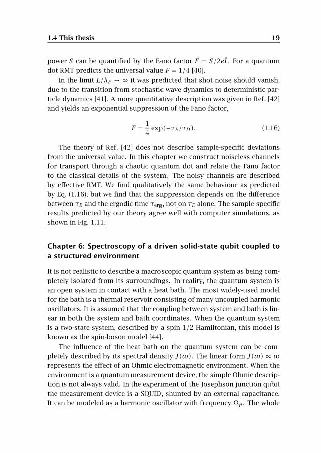
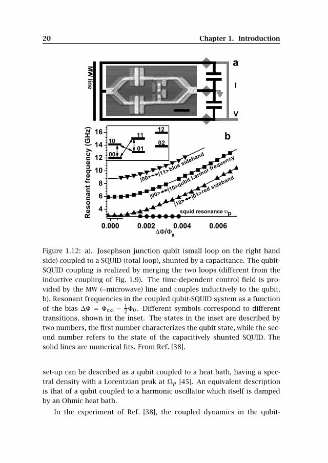
Figure 1.12: a). Josephson junction qubit (small loop on the right handside) coupled to a SQUID (total loop), shunted by a capacitance. The qubit-SQUID coupling is realized by merging the two loops (different from theinductive coupling of Fig. 1.9). The time-dependent control field is pro-vided by the MW (=microwave) line and couples inductively to the qubit.b). Resonant frequencies in the coupled qubit-SQUID system as a functionof the bias ∆Φ = Φext − 1
2Φ0. Different symbols correspond to differenttransitions, shown in the inset. The states in the inset are described bytwo numbers, the first number characterizes the qubit state, while the sec-ond number refers to the state of the capacitively shunted SQUID. Thesolid lines are numerical fits. From Ref. [38].
set-up can be described as a qubit coupled to a heat bath, having a spec-tral density with a Lorentzian peak at Ωp [45]. An equivalent descriptionis that of a qubit coupled to a harmonic oscillator which itself is dampedby an Ohmic heat bath.
In the experiment of Ref. [38], the coupled dynamics in the qubit-
1.4 This thesis 21
oscillator system was investigated (cf. Fig. 1.12). In this chapter we give aquantitative description of the behaviour of the system, both in the experi-mentally relevant weak damping limit and in the limit of strong dampingand/or high temperature. We find that the combination of the coupling tothe SQUID and the time-dependent control field results in resonances inthe long-time behaviour of the qubit, in agreement with the experiment.We give analytical formulas for their line-shapes. They compare well withthe results of a numerical ab-initio calculation.

22 Chapter 1. Introduction
Bibliography
[1] A. F. Andreev, Zh. Eksp. Teor. Fiz. 46, 1823 (1964) [Sov. Phys. JETP 19,1228 (1964)].
[2] P. G. de Gennes, Superconductivity of Metals and Alloys (Benjamin,New York, 1966).
[3] Y. Imry, Introduction to Mesoscopic Physics (Oxford University Press,Oxford, 1997).
[4] B. J. van Wees and H. Takayanagi, in Mesoscopic Electron Transport,edited by L. L. Sohn, L. P. Kouwenhoven, and G. Schon, NATO ASISeries E345 (Kluwer, Dordrecht, 1997).
[5] B. D. Josephson, Phys. Lett. 1, 251 (1962).
[6] M. Tinkham, Introduction to Superconductivity (McGraw-Hill, NewYork, 1996).
[7] I. O. Kulik, Zh. Eksp. Teor. Fiz. 57, 1745 (1969) [Sov. Phys. JETP 30,944 (1970)].
[8] J. A. Melsen, P. W. Brouwer, K. M. Frahm, and C. W. J. Beenakker,Europhys. Lett. 35, 7 (1996).
[9] A. J. Lichtenberg and M. A. Lieberman, Regular and Chaotic Dynamics(Springer, New York, 1983).
[10] M. C. Gutzwiller, Chaos in Classical and Quantum Mechanics(Springer, Berlin, 1990).
[11] E. Ott, Chaos in Dynamical Systems (Cambridge University Press, Cam-bridge, 1993).
24 Bibliography
[12] G. Casati and B. V. Chirikov, Quantum Chaos (Cambridge UniversityPress, Cambridge, 1995).
[13] H. -J. Stockmann, Quantum Chaos, An Introduction (Cambridge Uni-versity Press, Cambridge, 1999).
[14] F. Haake, Quantum Signatures of Chaos (Springer, Berlin, 2001).
[15] J. A. Melsen, P. W. Brouwer, K. M. Frahm, and C. W. J. Beenakker,Physica Scripta T69, 223 (1997).
[16] M. L. Mehta, Random Matrices (Academic Press, New York, 1991).
[17] C. W. J. Beenakker, Rev. Mod. Phys. 69, 731 (1997).
[18] T. Guhr, A. Muller-Groeling, and H. A. Weidenmuller, Phys. Rep. 299,189 (1998).
[19] I. Kosztin, D. L. Maslov, and P. M. Goldbart, Phys. Rev. Lett. 75, 1735(1995).
[20] H. Schomerus and C. W. J. Beenakker, Phys. Rev. Lett. 82, 2951 (1999).
[21] A. Lodder and Yu. V. Nazarov, Phys. Rev. B 58, 5783 (1998).
[22] P. Ehrenfest, Z. Phys. 45, 455 (1927).
[23] C. W. J. Beenakker, Lect. Notes Phys. 667, 131 (2005); cond-mat/0406018.
[24] Ph. Jacquod, H. Schomerus, and C. W. J. Beenakker, Phys. Rev. Lett.90, 207004 (2003).
[25] A. J. Leggett and A. Garg, Phys. Rev. Lett. 54, 857 (1985).
[26] M. A. Nielsen and I. L. Chuang, Quantum Computation and QuantumInformation (Cambridge University Press, Cambridge, 2000).
[27] D. P. DiVincenzo, in Mesoscopic Electron Transport, edited by L. L.Sohn, L. P. Kouwenhoven, and G. Schon, NATO ASI Series E345(Kluwer, Dordrecht, 1997); quant-ph/0002077.
[28] Y. Makhlin, G. Schon, and A. Shnirman, Rev. Mod. Phys. 73, 357 (2001).
Bibliography 25
[29] Y. Nakamura, Yu. A. Pashkin, and J. S. Tsai, Nature 398, 786 (1999).
[30] D. Vion, A. Aassime, A. Cottet, P. Joyez, H. Pothier, C. Urbina, D. Es-teve, and M. H. Devoret, Science 296, 886 (2002).
[31] Y. Yu, S. Y. Han, X. Chu, S. I. Chu, and Z. Wang, Science 296, 889(2002).
[32] J. M. Martinis, S. Nam, J. Aumentado, and C. Urbina, Phys. Rev. Lett.89, 117901 (2002).
[33] I. Chiorescu, Y. Nakamura, C. J. P. M. Harmans, and J. E Mooij, Science299, 1869 (2003).
[34] T. Duty, D. Gunnarsson, K. Bladh, and P. Delsing, Phys. Rev. B 69,140503(R) (2004).
[35] J. E. Mooij, T. P. Orlando, L. S. Levitov, L. Tian, C. H. van der Wal, andS. Lloyd, Science 285, 1036 (1999).
[36] C. H. van der Wal, Ph. D. thesis (2001).
[37] T. P. Orlando, J. E. Mooij, L. Tian, C. H. van der Wal, L. S. Levitov, S.Lloyd, and J. J. Mazo, Phys. Rev. B 60, 15398 (1999).
[38] I. Chiorescu, P. Bertet, K. Semba, Y. Nakamura, C. J. P. M. Harmans,and J. E. Mooij, Nature 431, 159 (2004).
[39] M. G. Vavilov, P. W. Brouwer, V. Ambegaokar, and C. W. J. Beenakker,Phys. Rev. Lett. 86, 874 (2001).
[40] R. A. Jalabert, J.-L. Pichard, and C. W. J. Beenakker, Europhys. Lett. 27,255 (1994).
[41] C. W. J. Beenakker and H. van Houten, Phys. Rev. B 43, 12066 (1991).
[42] O. Agam, I. Aleiner, and A. Larkin, Phys. Rev. Lett. 85, 3153 (2000).
[43] J. Tworzydło, A. Tajic, H. Schomerus, and C. W. J. Beenakker, Phys.Rev. B 68, 115313 (2003).
[44] U. Weiss, Quantum Dissipative Systems (World Scienific, Singapore,1999).

26 Bibliography
[45] L. Tian, S. Lloyd, and T. P. Orlando, Phys. Rev. B 65, 144516 (2002).
Chapter 2
Adiabatic quantization of an
Andreev billiard
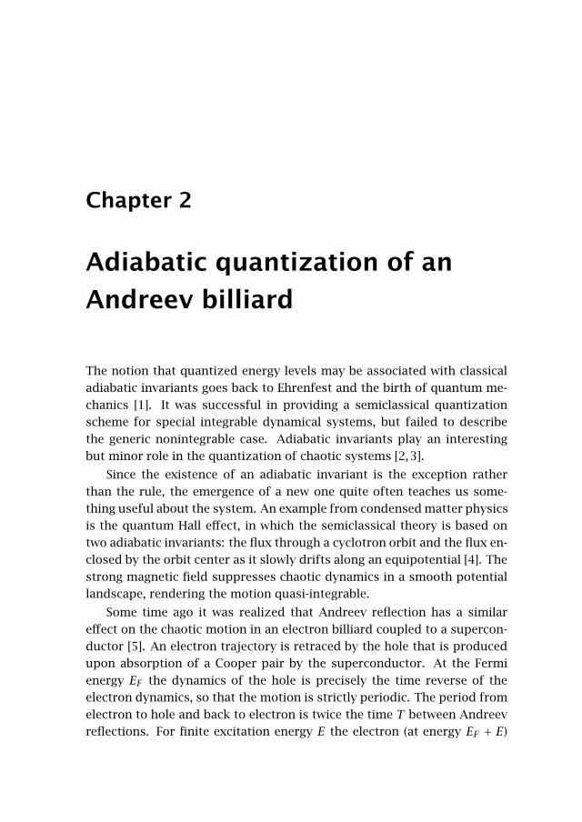
The notion that quantized energy levels may be associated with classicaladiabatic invariants goes back to Ehrenfest and the birth of quantum me-chanics [1]. It was successful in providing a semiclassical quantizationscheme for special integrable dynamical systems, but failed to describethe generic nonintegrable case. Adiabatic invariants play an interestingbut minor role in the quantization of chaotic systems [2,3].
Since the existence of an adiabatic invariant is the exception ratherthan the rule, the emergence of a new one quite often teaches us some-thing useful about the system. An example from condensed matter physicsis the quantum Hall effect, in which the semiclassical theory is based ontwo adiabatic invariants: the flux through a cyclotron orbit and the flux en-closed by the orbit center as it slowly drifts along an equipotential [4]. Thestrong magnetic field suppresses chaotic dynamics in a smooth potentiallandscape, rendering the motion quasi-integrable.
Some time ago it was realized that Andreev reflection has a similareffect on the chaotic motion in an electron billiard coupled to a supercon-ductor [5]. An electron trajectory is retraced by the hole that is producedupon absorption of a Cooper pair by the superconductor. At the Fermienergy EF the dynamics of the hole is precisely the time reverse of theelectron dynamics, so that the motion is strictly periodic. The period fromelectron to hole and back to electron is twice the time T between Andreevreflections. For finite excitation energy E the electron (at energy EF + E)
28 Chapter 2. Adiabatic quantization . . .
and the hole (at energy EF − E) follow slightly different trajectories, so theorbit does not quite close and drifts around in phase space. This drifthas been studied in a variety of contexts [5–9], but not in connection withadiabatic invariants and the associated quantization conditions. It is thepurpose of this chapter to make that connection and point out a strikingphysical consequence: The wave functions of adiabatically quantized An-dreev levels fill the cavity in a highly nonuniform “squeezed” way, whichhas no counterpart in normal state chaotic or regular billiards. In particu-lar the squeezing is distinct from periodic orbit scarring [10] and entirelydifferent from the random superposition of plane waves expected for afully chaotic billiard [11].
Adiabatic quantization breaks down near the excitation gap, and wewill argue that random-matrix theory [12] can be used to quantize thelowest-lying excitations above the gap. This will lead us to a formula forthe gap that crosses over from the Thouless energy to the inverse Ehren-fest time as the number of modes in the point contact is increased.
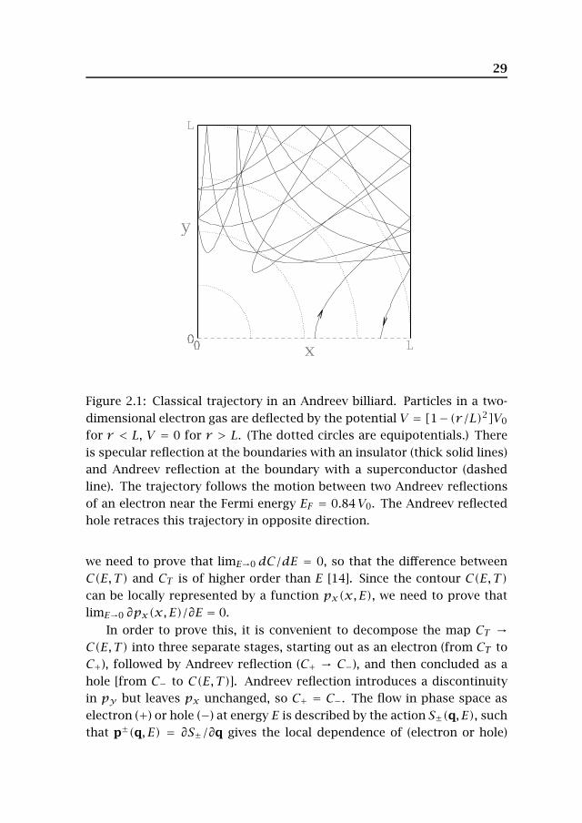
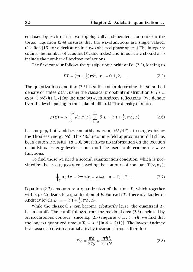
To illustrate the problem we represent in Figs. 2.1 and 2.2 the quasiperi-odic motion in a particular Andreev billiard. (It is similar to a Sinai billiard,but has a smooth potential V in the interior to favor adiabaticity.) Figure2.1 shows a trajectory in real space while Fig. 2.2 is a section of phasespace at the interface with the superconductor (y = 0). The tangentialcomponent px of the electron momentum is plotted as a function of thecoordinate x along the interface. Each point in this Poincare map corre-sponds to one collision of an electron with the interface. (The collisionsof holes are not plotted.) The electron is retroreflected as a hole with thesame px. At E = 0 the component py is also the same, and so the holeretraces the path of the electron (the hole velocity being opposite to itsmomentum). At non-zero E the retroreflection occurs with a slight changein py , because of the difference 2E in the kinetic energy of electrons andholes. The resulting slow drift of the periodic trajectory traces out a con-tour in the surface of section. The adiabatic invariant is the function ofx,px that is constant on the contour. We have found numerically that thedrift follows isochronous contours CT of constant time T(x,px) betweenAndreev reflections [13]. Let us now demonstrate analytically that T is anadiabatic invariant.
We consider the Poincare map CT → C(E, T) at energy E. If E = 0 thePoincare map is the identity, so C(0, T) = CT . For adiabatic invariance
29
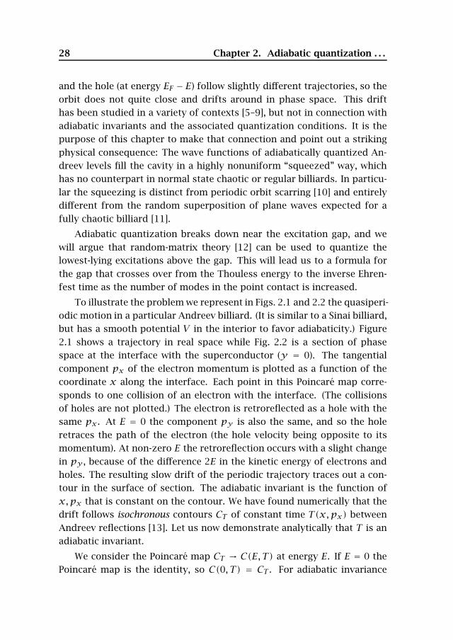
Figure 2.1: Classical trajectory in an Andreev billiard. Particles in a two-dimensional electron gas are deflected by the potential V = [1−(r/L)2]V0
for r < L, V = 0 for r > L. (The dotted circles are equipotentials.) Thereis specular reflection at the boundaries with an insulator (thick solid lines)and Andreev reflection at the boundary with a superconductor (dashedline). The trajectory follows the motion between two Andreev reflectionsof an electron near the Fermi energy EF = 0.84V0. The Andreev reflectedhole retraces this trajectory in opposite direction.
we need to prove that limE→0 dC/dE = 0, so that the difference betweenC(E, T) and CT is of higher order than E [14]. Since the contour C(E, T)can be locally represented by a function px(x,E), we need to prove thatlimE→0 ∂px(x, E)/∂E = 0.
In order to prove this, it is convenient to decompose the map CT →C(E, T) into three separate stages, starting out as an electron (from CT toC+), followed by Andreev reflection (C+ → C−), and then concluded as ahole [from C− to C(E, T)]. Andreev reflection introduces a discontinuityin py but leaves px unchanged, so C+ = C−. The flow in phase space aselectron (+) or hole (−) at energy E is described by the action S±(q, E), suchthat p±(q, E) = ∂S±/∂q gives the local dependence of (electron or hole)
30 Chapter 2. Adiabatic quantization . . .
Figure 2.2: Poincare map for the Andreev billiard of Fig. 2.1. Each dotrepresents a starting point of an electron trajectory, at position x (in unitsof L) along the interface y = 0 and with tangential momentum px (in unitsof√mV0). The inset shows the full surface of section, while the main plot
is an enlargement of the central region. The drifting quasiperiodic motionfollows contours of constant time T between Andreev reflections. Thecross marks the starting point of the trajectory shown in the previous
figure, having T = 18 (in units of√mL2/V0).
momentum p = (px,py) on position q = (x,y). The derivative ∂S±/∂E =t±(q, E) is the time elapsed since the previous Andreev reflection. Sinceby construction t±(x,y = 0, E = 0) = T is independent of the position xof the end of the trajectory, we find that limE→0 ∂p±x (x,y = 0, E)/∂E = 0,completing the proof.
The drift (δx,δpx) of a point in the Poincare map is perpendicular tothe vector (∂T/∂x, ∂T/∂px). Using also that the map is area preserving, itfollows that
(δx,δpx) = Ef(T)(∂T/∂px,−∂T/∂x) +O(E2), (2.1)
with a prefactor f(T) that is the same along the entire contour.
31
The adiabatic invariance of isochronous contours may alternatively beobtained from the adiabatic invariance of the action integral I over thequasiperiodic motion from electron to hole and back to electron:
I =∮pdq = E
∮dqq= 2ET. (2.2)
Since E is a constant of the motion, adiabatic invariance of I implies adia-batic invariance of the time T between Andreev reflections. This is the wayin which adiabatic invariance is usually proven in textbooks. Our proof ex-plicitly takes into account the fact that phase space in the Andreev billiardconsists of two sheets, joined in the constriction at the interface with thesuperconductor, with a discontinuity in the action on going from one sheetto the other.
The contours of large T enclose a very small area. This will play a cru-cial role when we quantize the billiard, so let us estimate the area. Elec-trons leaving the superconductor have transverse momenta in the range(−pW ,pW), with the value of pW depending on the details of the potentialnear the superconductor. It is convenient for our estimate to measure pxand x in units of pW and the width W of the constriction to the super-conductor [15]. The highly elongated shape evident in Fig. 2.2 is a conse-quence of the exponential divergence in time of nearby trajectories, char-acteristic of chaotic dynamics. The rate of divergence is the Lyapunov ex-ponent λ. (We consider a fully chaotic phase space.) Since the Hamiltonianflow is area preserving, a stretching +(t) = +(0)eλt of the dimension inone direction needs to be compensated by a squeezing −(t) = −(0)e−λtof the dimension in the other direction. The area O(t) +(t)−(t) isthen time-independent. Initially, ±(0) < 1. The constriction at the super-conductor acts as a bottleneck, enforcing ±(T) < 1. These two inequali-ties imply +(t) < eλ(t−T), −(t) < e−λt . Therefore, the enclosed area hasupper bound
Omax pWWe−λT Ne−λT , (2.3)
where N pWW/ 1 is the number of channels in the point contact.We now continue with the quantization. The two invariants E and T de-
fine a two-dimensional torus in the four-dimensional phase space. Quan-tization of this adiabatically invariant torus proceeds following Einstein-Brillouin-Keller [3], by quantizing the area∮
pdq = 2π(m + ν/4), m = 0,1,2, . . . (2.4)
32 Chapter 2. Adiabatic quantization . . .
enclosed by each of the two topologically independent contours on thetorus. Equation (2.4) ensures that the wavefunctions are single valued.(See Ref. [16] for a derivation in a two-sheeted phase space.) The integer νcounts the number of caustics (Maslov index) and in our case should alsoinclude the number of Andreev reflections.
The first contour follows the quasiperiodic orbit of Eq. (2.2), leading to
ET = (m+ 12)π, m = 0,1,2, . . . (2.5)
The quantization condition (2.5) is sufficient to determine the smootheddensity of states ρ(E), using the classical probability distribution P(T) ∝exp(−TNδ/h) [17] for the time between Andreev reflections. (We denoteby δ the level spacing in the isolated billiard.) The density of states
ρ(E) = N∫∞
0dT P(T)
∞∑m=0
δ(E − (m+ 1
2)π/T)
(2.6)
has no gap, but vanishes smoothly ∝ exp(−Nδ/4E) at energies belowthe Thouless energy Nδ. This “Bohr-Sommerfeld approximation” [12] hasbeen quite successful [18–20], but it gives no information on the locationof individual energy levels — nor can it be used to determine the wavefunctions.
To find these we need a second quantization condition, which is pro-vided by the area
∮T pxdx enclosed by the contours of constant T(x,px),
∮Tpxdx = 2π(n+ ν/4), n = 0,1,2, . . . (2.7)
Equation (2.7) amounts to a quantization of the time T , which togetherwith Eq. (2.5) leads to a quantization of E. For each Tn there is a ladder ofAndreev levels Enm = (m+ 1
2)π/Tn.
While the classical T can become arbitrarily large, the quantized Tnhas a cutoff. The cutoff follows from the maximal area (2.3) enclosed byan isochronous contour. Since Eq. (2.7) requires Omax > π, we find thatthe longest quantized time is T0 = λ−1[lnN + O(1)]. The lowest Andreevlevel associated with an adiabatically invariant torus is therefore
E00 = π2T0 πλ
2 lnN. (2.8)
33
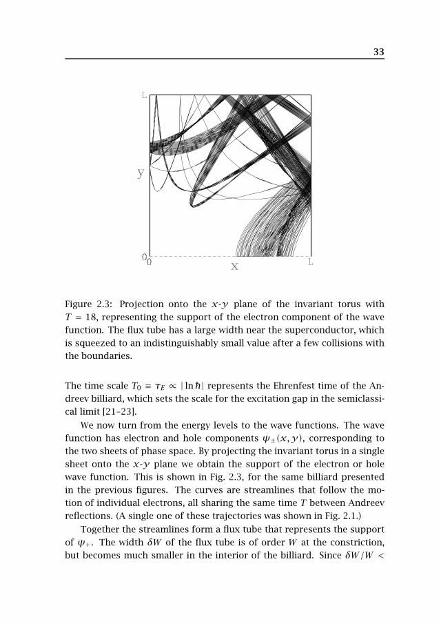
Figure 2.3: Projection onto the x-y plane of the invariant torus withT = 18, representing the support of the electron component of the wavefunction. The flux tube has a large width near the superconductor, whichis squeezed to an indistinguishably small value after a few collisions withthe boundaries.
The time scale T0 ≡ τE ∝ | ln| represents the Ehrenfest time of the An-dreev billiard, which sets the scale for the excitation gap in the semiclassi-cal limit [21–23].
We now turn from the energy levels to the wave functions. The wavefunction has electron and hole components ψ±(x,y), corresponding tothe two sheets of phase space. By projecting the invariant torus in a singlesheet onto the x-y plane we obtain the support of the electron or holewave function. This is shown in Fig. 2.3, for the same billiard presentedin the previous figures. The curves are streamlines that follow the mo-tion of individual electrons, all sharing the same time T between Andreevreflections. (A single one of these trajectories was shown in Fig. 2.1.)
Together the streamlines form a flux tube that represents the supportof ψ+. The width δW of the flux tube is of order W at the constriction,but becomes much smaller in the interior of the billiard. Since δW/W <
34 Chapter 2. Adiabatic quantization . . .
+ + − < eλ(t−T) + e−λt (with 0 < t < T ), we conclude that the flux tube issqueezed down to a width
δWmin We−λT/2. (2.9)
The flux tube for the level E00 has a minimal width δWmin W/√N. Parti-
cle conservation implies that |ψ+|2 ∝ 1/δW , so that the squeezing of theflux tube is associated with an increase of the electron density by a factorof√N as one moves away from the constriction.
Let us examine the range of validity of adiabatic quantization. The driftδx, δpx upon one iteration of the Poincare map should be small comparedto W,pF . We estimate
δxW
δpxpW
EnmλN
eλTn (m+ 12)e−λ(T0−Tn)
λTn. (2.10)
For low-lying levels (m ∼ 1) the dimensionless drift is 1 for Tn < T0.Even for Tn = T0 one has δx/W 1/ lnN 1.
Semiclassical methods allow to quantize only the trajectories with timesT ≤ T0 = τE . We propose that the part of phase space with longer periodscan be quantized by random-matrix theory (RMT). Since the RMT descrip-tion is only valid for a reduced phase space, we call it an effective RMT.
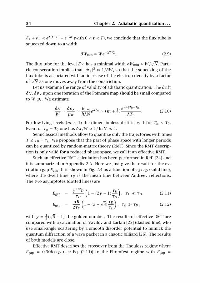
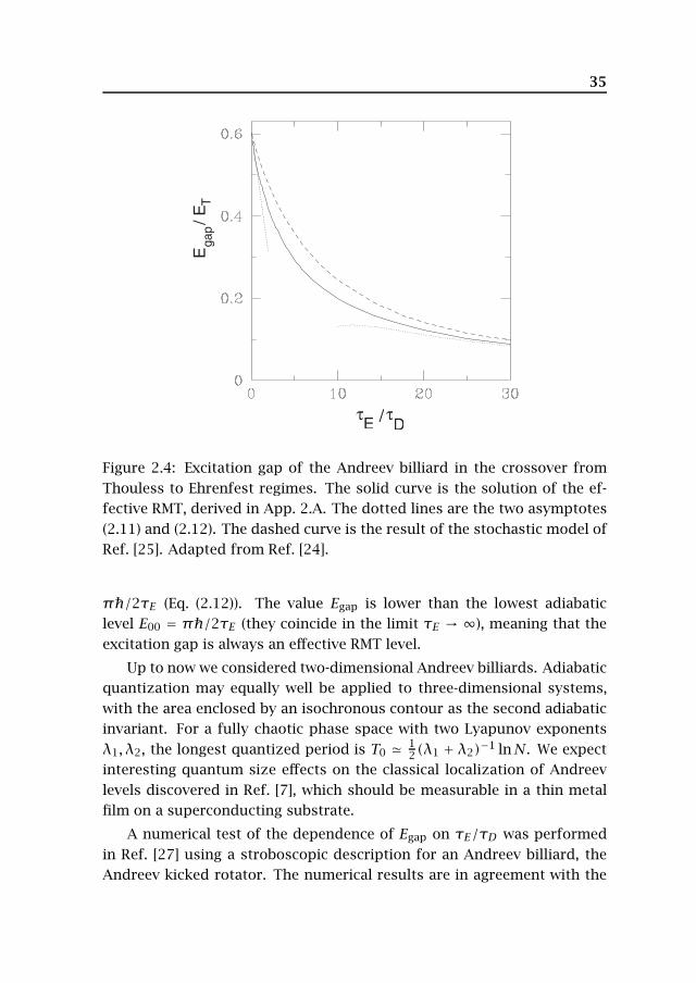
Such an effective RMT calculation has been performed in Ref. [24] andit is summarized in Appendix 2.A. Here we just give the result for the ex-citation gap Egap. It is shown in Fig. 2.4 as a function of τE/τD (solid line),where the dwell time τD is the mean time between Andreev reflections.The two asymptotes (dotted lines) are
Egap = γ5/2τD
(1− (2γ − 1)
τEτD
), τE τD, (2.11)
Egap = π2τE
(1− (3+
√8)τDτE
), τE τD, (2.12)
with γ = 12(√
5 − 1) the golden number. The results of effective RMT arecompared with a calculation of Vavilov and Larkin [25] (dashed line), whouse small-angle scattering by a smooth disorder potential to mimick thequantum diffraction of a wave packet in a chaotic billiard [26]. The resultsof both models are close.
Effective RMT describes the crossover from the Thouless regime whereEgap = 0.30/τD (see Eq. (2.11)) to the Ehrenfest regime with Egap =
35
/τD
τE
E
/ E
ga
pT
Figure 2.4: Excitation gap of the Andreev billiard in the crossover fromThouless to Ehrenfest regimes. The solid curve is the solution of the ef-fective RMT, derived in App. 2.A. The dotted lines are the two asymptotes(2.11) and (2.12). The dashed curve is the result of the stochastic model ofRef. [25]. Adapted from Ref. [24].
π/2τE (Eq. (2.12)). The value Egap is lower than the lowest adiabaticlevel E00 = π/2τE (they coincide in the limit τE → ∞), meaning that theexcitation gap is always an effective RMT level.
Up to now we considered two-dimensional Andreev billiards. Adiabaticquantization may equally well be applied to three-dimensional systems,with the area enclosed by an isochronous contour as the second adiabaticinvariant. For a fully chaotic phase space with two Lyapunov exponentsλ1, λ2, the longest quantized period is T0 1
2(λ1 + λ2)−1 lnN. We expectinteresting quantum size effects on the classical localization of Andreevlevels discovered in Ref. [7], which should be measurable in a thin metalfilm on a superconducting substrate.
A numerical test of the dependence of Egap on τE/τD was performedin Ref. [27] using a stroboscopic description for an Andreev billiard, theAndreev kicked rotator. The numerical results are in agreement with the
36 Chapter 2. Adiabatic quantization . . .
effective RMT prediction of Egap (see Ref. [24] for a comparison). In theAndreev kicked rotator the drift due to a finite excitation energy E wasnot included and adiabatic levels were not considered. One importantchallenge for future research is to test the adiabatic quantization of An-dreev levels numerically, by solving the Bogoliubov-De Gennes equationon a computer. The characteristic signature of the adiabatic invariant thatwe have discovered, a narrow region of enhanced intensity in a chaotic re-gion that is squeezed as one moves away from the superconductor, shouldbe readily observable and distinguishable from other features that are un-related to the presence of the superconductor, such as scars of unstableperiodic orbits [10]. Experimentally these regions might be observable us-ing a scanning tunneling probe, which provides an energy and spatiallyresolved measurement of the electron density.
2.A Effective RMT
In this appendix we summarize the effective RMT calculation of Ref. [24].Effective RMT is based on the hypothesis that the part of phase space withlong trajectories can be quantized by a scattering matrix Sq in the circularensemble of RMT, with a reduced dimensionality
Neff = N∫∞τEP(T)dT = Ne−τE/τD . (2.13)
The energy dependence of Sq(E) is that of a chaotic cavity with meanlevel spacing δeff, coupled to the superconductor by a long lead withNeff propagating modes. (See Fig. 2.5.) The lead introduces a mode-independent delay time τE between Andreev reflections, to ensure thatP(T) is cut off for T < τE . Because P(T) is exponential ∝ exp(−T/τD),the mean time 〈T〉∗ between Andreev reflections in the accessible part ofphase space is simply τE + τD . The effective level spacing in the chaoticcavity by itself (without the lead) is then determined by
2πNeffδeff
= 〈T〉∗ − τE = τD. (2.14)
It is convenient to separate the energy dependence due to the leadfrom that due to the cavity, by writing Sq(E) = exp(iEτE/)S0(E). Theunitary symmetric matrix S0 corresponds to a chaotic cavity with effective
2.A Effective RMT 37
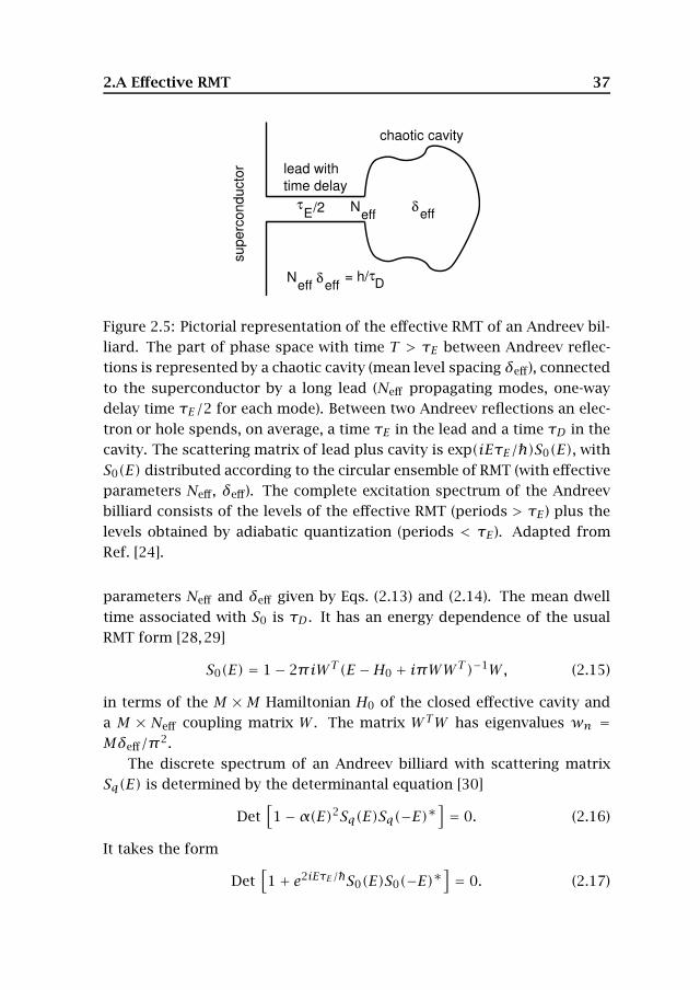
Figure 2.5: Pictorial representation of the effective RMT of an Andreev bil-liard. The part of phase space with time T > τE between Andreev reflec-tions is represented by a chaotic cavity (mean level spacing δeff), connectedto the superconductor by a long lead (Neff propagating modes, one-waydelay time τE/2 for each mode). Between two Andreev reflections an elec-tron or hole spends, on average, a time τE in the lead and a time τD in thecavity. The scattering matrix of lead plus cavity is exp(iEτE/)S0(E), withS0(E) distributed according to the circular ensemble of RMT (with effectiveparameters Neff, δeff). The complete excitation spectrum of the Andreevbilliard consists of the levels of the effective RMT (periods > τE ) plus thelevels obtained by adiabatic quantization (periods < τE). Adapted fromRef. [24].
parameters Neff and δeff given by Eqs. (2.13) and (2.14). The mean dwelltime associated with S0 is τD . It has an energy dependence of the usualRMT form [28,29]
S0(E) = 1− 2πiWT(E −H0 + iπWWT)−1W, (2.15)
in terms of the M ×M Hamiltonian H0 of the closed effective cavity anda M × Neff coupling matrix W . The matrix WTW has eigenvalues wn =Mδeff/π2.
The discrete spectrum of an Andreev billiard with scattering matrixSq(E) is determined by the determinantal equation [30]
Det[1−α(E)2Sq(E)Sq(−E)∗
]= 0. (2.16)
It takes the form
Det[1+ e2iEτE/S0(E)S0(−E)∗
]= 0. (2.17)
38 Chapter 2. Adiabatic quantization . . .
We have replaced α(E) ≡ exp[−i arccos(E/∆)] → −i (since E ∆), butthe energy dependence of the phase factor e2iEτE/ can not be omitted.The calculation for Neff 1 follows the method described in Ref. [12],modified as in Ref. [31] to account for the energy dependent phase factorin the determinant.
Using Eq. (2.15), we can write Eq. (2.17) in the Hamiltonian form
Det [E −Heff] = 0, (2.18)
Heff =(H0 00 −H∗0
)−W(E), (2.19)
W(E) = πcosu
(WWT sinu WWT
WWT WWT sinu
), (2.20)
where we have abbreviated u = EτE/. The ensemble averaged density ofstates is given by
ρeff(E) = −1π
Im Tr(
1+ dWdE
)〈(E + i0+ −Heff)−1〉. (2.21)
In the presence of time-reversal symmetry the Hamiltonian H0 of theisolated billiard is a real symmetric matrix. The appropriate RMT ensembleis the GOE, with distribution [32]
P(H) ∝ exp
(− π2
4Mδ2eff
TrH2
). (2.22)
The ensemble average 〈· · · 〉 in Eq. 2.21 is an average over H0 in the GOEat fixed coupling matrix W . Because of the block structure of Heff, theensemble averaged Green function G(E) = 〈(E −Heff)−1〉 consists of fourM ×M blocks G11, G12, G21, G22. By taking the trace of each block sepa-rately, one arrives at a 2× 2 matrix Green function
G =(G11 G12
G21 G22
)= δπ
(TrG11 TrG12
TrG21 TrG22
). (2.23)
(The factor δ/π is inserted for later convenience.)The average over the distribution (2.22) can be done diagrammatically
[33, 34]. To leading order in 1/M and for E δ only simple (planar)diagrams need to be considered. Resummation of these diagrams leads tothe selfconsistency equation [12,31]
G = [E +W − (Mδeff/π)σzGσz]−1, σz =(
1 00 −1
). (2.24)
2.A Effective RMT 39
After some algebra we find that G22 = G11 and G21 = G12 and there aretwo unknown functions to determine. For M N these satisfy
G212 = 1+G2
11, (2.25a)
G11 +G12 sinu = −(τD/τE)uG12
× (G12 + cosu+G11 sinu). (2.25b)
and the density of states (2.21) is given by
ρeff(E) = −2δeff
Im(G11 − u
cosuG12
). (2.26)
The excitation gap corresponds to a square root singularity in ρeff(E),which can be obtained by solving Eqs. (2.25a) and (2.25b) jointly withdE/dG11 = 0 for u ∈ (0, π/2). The result is plotted in Fig. 2.4. Thesmall- and large-τE asymptotes are given by Eqs. (2.11) and (2.12).

40 Chapter 2. Adiabatic quantization . . .
Bibliography
[1] P. Ehrenfest, Ann. Phys. (Leipzig) 51, 327 (1916).
[2] C. C. Martens, R. L. Waterland, and W. P. Reinhardt, J. Chem. Phys. 90,2328 (1989).
[3] M. C. Gutzwiller, Chaos in Classical and Quantum Mechanics(Springer, Berlin, 1990).
[4] R. E. Prange, in The Quantum Hall Effect, edited by R. E. Prange and S.M. Girvin (Springer, New York, 1990).
[5] I. Kosztin, D. L. Maslov, and P. M. Goldbart, Phys. Rev. Lett. 75, 1735(1995).
[6] M. Stone, Phys. Rev. B 54, 13222 (1996).
[7] A. V. Shytov, P. A. Lee, and L. S. Levitov, Phys. Uspekhi 41, 207 (1998).
[8] I. Adagideli and P. M. Goldbart, Phys. Rev. B 65, 201306 (2002).
[9] J. Wiersig, Phys. Rev. E 65, 036221 (2002).
[10] E. J. Heller, Phys. Rev. Lett. 53, 1515 (1984).
[11] P. W. O’Connor, J. Gehlen, and E. Heller, Phys. Rev. Lett. 58, 1296(1987).
[12] J. A. Melsen, P. W. Brouwer, K. M. Frahm, and C. W. J. Beenakker,Europhys. Lett. 35, 7 (1996).
[13] Isochronous contours are defined as T(x,px) = constant at E = 0. Weassume that the isochronous contours are closed. This is true if the
42 Bibliography
border py = 0 of the classically allowed region in the x,px section isitself an isochronous contour, which is the case if limy→0 ∂V/∂y ≤ 0.In this case the particle leaving the superconductor with infinitesimalpy can not penetrate into the billiard.
[14] Adiabatic invariance is defined in the limit E → 0 and is there-fore distinct from invariance in the sense of Kolmogorov-Arnold-Moser (KAM), which would require a critical E∗ such that a contour isexactly invariant for E < E∗. Numerical evidence [5] suggests that theKAM theorem does not apply to a chaotic Andreev billiard.
[15] In this chapter we assume that pW/pF W/L, which is typical of asmooth confining potential. In the case W/L pW/pF , typical fora hard wall potential and for the computer simulations with the An-dreev kicked rotator of Ref. [27], the area Omax is larger by a factorW/L (see chapter 5). Consequently the factor lnN in Eq. (2.8) shouldbe replaced by ln(NW/L).
[16] K. P. Duncan and B. L. Gyorffy, Ann. Phys. (New York) 298, 273 (2002).
[17] W. Bauer and G. F. Bertsch, Phys. Rev. Lett., 65, 2213 (1990).
[18] H. Schomerus and C. W. J. Beenakker, Phys. Rev. Lett. 82, 2951 (1999).
[19] W. Ihra, M. Leadbeater, J. L. Vega, and K. Richter, Europhys. J. B 21,425 (2001).
[20] J. Cserti, A. Kormanyos, Z. Kaufmann, J Koltai, and C. J. Lambert,Phys. Rev. Lett. 89, 057001 (2002).
[21] A. Lodder and Yu. V. Nazarov, Phys. Rev. B 58, 5783 (1998).
[22] D. Taras-Semchuk and A. Altland, Phys. Rev. B 64, 014512 (2001).
[23] I. Adagideli and C. W. J. Beenakker, Phys. Rev. Lett. 89, 237002 (2002).
[24] C. W. J. Beenakker, Lect. Notes Phys. 667, 131 (2005); cond-mat/0406018.
[25] M. G. Vavilov and A. I. Larkin, Phys. Rev. B 67, 115335 (2003).
[26] I. L. Aleiner and A. I. Larkin, Phys. Rev. B 55, 1243 (1997).
Bibliography 43
[27] Ph. Jacquod, H. Schomerus, and C. W. J. Beenakker, Phys. Rev. Lett.90, 207004 (2003).
[28] T. Guhr, A. Muller-Groeling, and H. A. Weidenmuller, Phys. Rep. 299,189 (1998).
[29] C. W. J. Beenakker, Rev. Mod. Phys. 69, 731 (1997).
[30] C. W. J. Beenakker, Phys. Rev. Lett. 67, 3836 (1991); 68, 1442(E) (1992).
[31] P. W. Brouwer and C. W. J. Beenakker, Chaos, Solitons & Fractals 8,1249 (1997).
[32] M. L. Mehta, Random Matrices (Academic, New York, 1991).
[33] A. Pandey, Ann. Phys. (N.Y.) 134, 110 (1981).
[34] E. Brezin and A. Zee, Phys. Rev. E 49, 2588 (1994).

44 Bibliography
Chapter 3
Quasiclassical fluctuations of
the superconductor proximity
gap in a chaotic system
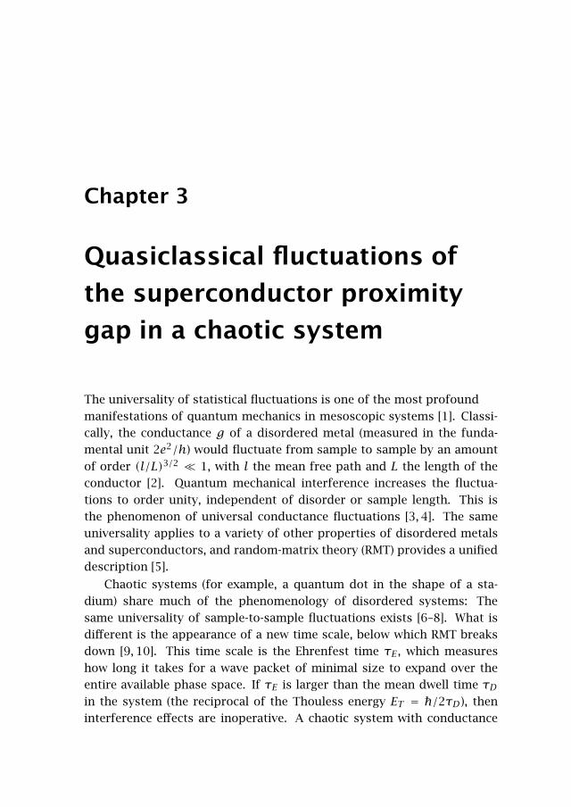
The universality of statistical fluctuations is one of the most profoundmanifestations of quantum mechanics in mesoscopic systems [1]. Classi-cally, the conductance g of a disordered metal (measured in the funda-mental unit 2e2/h) would fluctuate from sample to sample by an amountof order (l/L)3/2 1, with l the mean free path and L the length of theconductor [2]. Quantum mechanical interference increases the fluctua-tions to order unity, independent of disorder or sample length. This isthe phenomenon of universal conductance fluctuations [3, 4]. The sameuniversality applies to a variety of other properties of disordered metalsand superconductors, and random-matrix theory (RMT) provides a unifieddescription [5].
Chaotic systems (for example, a quantum dot in the shape of a sta-dium) share much of the phenomenology of disordered systems: Thesame universality of sample-to-sample fluctuations exists [6–8]. What isdifferent is the appearance of a new time scale, below which RMT breaksdown [9, 10]. This time scale is the Ehrenfest time τE , which measureshow long it takes for a wave packet of minimal size to expand over theentire available phase space. If τE is larger than the mean dwell time τDin the system (the reciprocal of the Thouless energy ET = /2τD), theninterference effects are inoperative. A chaotic system with conductance
46 Chapter 3. Quasiclassical fluctuations . . .
g × 2e2/h, level spacing δ, and Lyapunov exponent λ has τD = 2π/gδand τE = λ−1
[ln (gτ0/τD)+O(1)
], with τ0 the time of flight across the
system [11]. The defining characteristic of the Ehrenfest time is that itscales logarithmically with , or equivalently, logarithmically with the sys-tem size over Fermi wavelength [12].
The purpose of this chapter is to investigate what happens to meso-scopic fluctuations if the Ehrenfest time becomes comparable to, or largerthan, the dwell time, so one enters a quasiclassical regime where RMT nolonger holds. This quasiclassical regime has not yet been explored experi-mentally. The difficulty is that τE increases so slowly with system sizethat the averaging effects of inelastic scattering take over before the effectof a finite Ehrenfest time can be seen. In a computer simulation inelasticscattering can be excluded from the model by construction, so this seemsa promising alternative to investigate the crossover from universal quan-tum fluctuations to nonuniversal quasiclassical fluctuations. Contrary towhat one would expect from the disordered metal [2], where quasiclassi-cal fluctuations are much smaller than the quantum value, we find thatthe breakdown of universality in the chaotic system is associated with anenhancement of the sample-to-sample fluctuations.
The quantity on which we choose to focus is the excitation gap E0 ofa chaotic system which is weakly coupled to a superconductor. We havetwo reasons for this choice: Firstly, there exists a model (the Andreevkicked rotator) which permits a computer simulation for systems largeenough that τE τD . So far, such simulations, have confirmed the theoryof Ref. [11] for the average gap 〈E0〉 [13]. Secondly, the quasiclassicaltheory of chapter 2 can describe the effect of a finite Ehrenfest time onthe excitation gap and its fluctuations. This allows us to achieve both anumerical and an analytical understanding of the mesoscopic fluctuationswhen RMT breaks down.
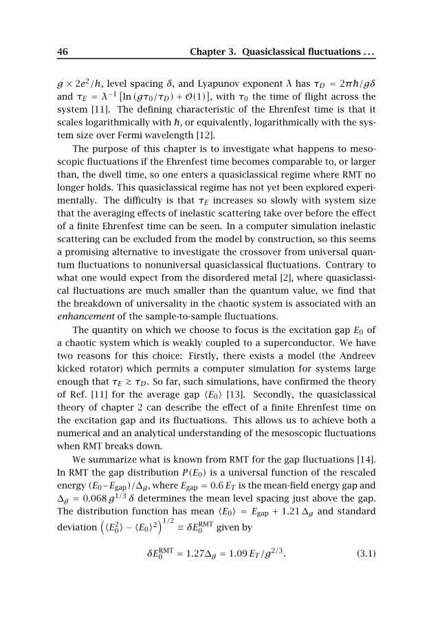
We summarize what is known from RMT for the gap fluctuations [14].In RMT the gap distribution P(E0) is a universal function of the rescaledenergy (E0−Egap)/∆g , where Egap = 0.6ET is the mean-field energy gap and∆g = 0.068g1/3 δ determines the mean level spacing just above the gap.The distribution function has mean 〈E0〉 = Egap + 1.21∆g and standard
deviation(〈E2
0〉 − 〈E0〉2)1/2 ≡ δERMT
0 given by
δERMT0 = 1.27∆g = 1.09ET/g2/3. (3.1)
47
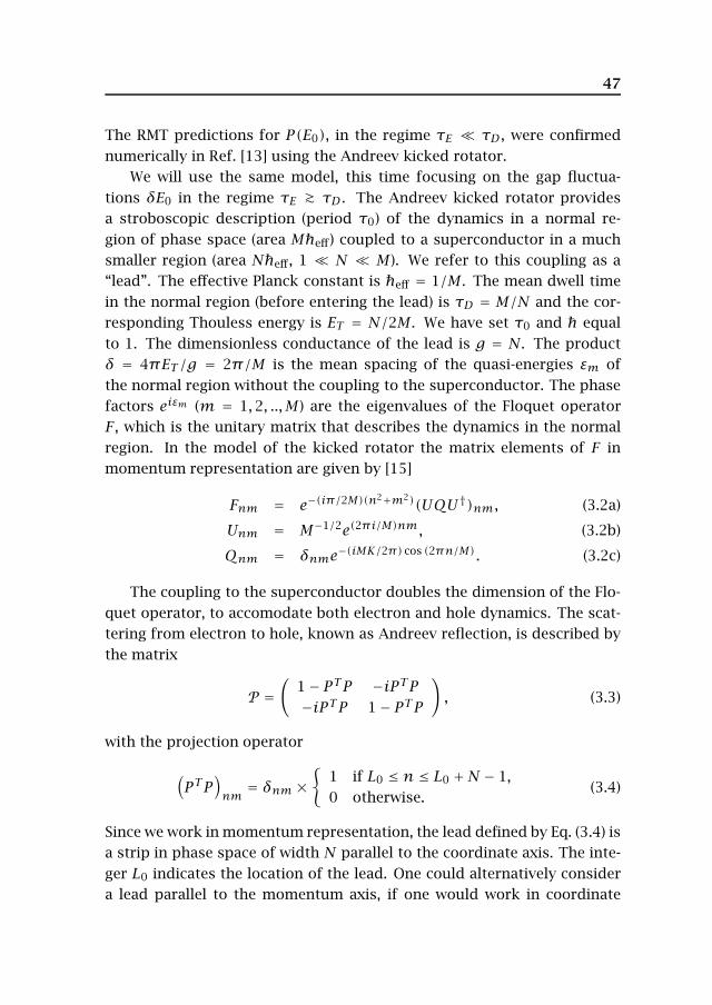
The RMT predictions for P(E0), in the regime τE τD , were confirmednumerically in Ref. [13] using the Andreev kicked rotator.
We will use the same model, this time focusing on the gap fluctua-tions δE0 in the regime τE τD . The Andreev kicked rotator providesa stroboscopic description (period τ0) of the dynamics in a normal re-gion of phase space (area Meff) coupled to a superconductor in a muchsmaller region (area Neff, 1 N M). We refer to this coupling as a“lead”. The effective Planck constant is eff = 1/M . The mean dwell timein the normal region (before entering the lead) is τD = M/N and the cor-responding Thouless energy is ET = N/2M . We have set τ0 and equalto 1. The dimensionless conductance of the lead is g = N. The productδ = 4πET/g = 2π/M is the mean spacing of the quasi-energies εm ofthe normal region without the coupling to the superconductor. The phasefactors eiεm (m = 1,2, ..,M) are the eigenvalues of the Floquet operatorF , which is the unitary matrix that describes the dynamics in the normalregion. In the model of the kicked rotator the matrix elements of F inmomentum representation are given by [15]
Fnm = e−(iπ/2M)(n2+m2)(UQU†)nm, (3.2a)
Unm = M−1/2e(2πi/M)nm, (3.2b)
Qnm = δnme−(iMK/2π) cos (2πn/M). (3.2c)
The coupling to the superconductor doubles the dimension of the Flo-quet operator, to accomodate both electron and hole dynamics. The scat-tering from electron to hole, known as Andreev reflection, is described bythe matrix
P =(
1− PTP −iPTP−iPTP 1− PTP
), (3.3)
with the projection operator
(PTP
)nm
= δnm ×
1 if L0 ≤ n ≤ L0 +N − 1,0 otherwise.
(3.4)
Since we work in momentum representation, the lead defined by Eq. (3.4) isa strip in phase space of width N parallel to the coordinate axis. The inte-ger L0 indicates the location of the lead. One could alternatively considera lead parallel to the momentum axis, if one would work in coordinate
48 Chapter 3. Quasiclassical fluctuations . . .
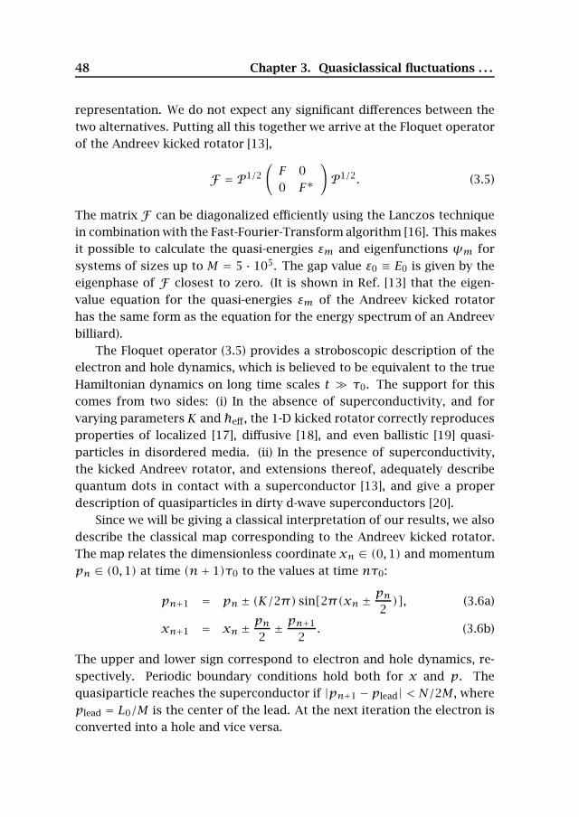
representation. We do not expect any significant differences between thetwo alternatives. Putting all this together we arrive at the Floquet operatorof the Andreev kicked rotator [13],
F = P1/2(F 00 F∗
)P1/2. (3.5)
The matrix F can be diagonalized efficiently using the Lanczos techniquein combination with the Fast-Fourier-Transform algorithm [16]. This makesit possible to calculate the quasi-energies εm and eigenfunctions ψm forsystems of sizes up to M = 5 · 105. The gap value ε0 ≡ E0 is given by theeigenphase of F closest to zero. (It is shown in Ref. [13] that the eigen-value equation for the quasi-energies εm of the Andreev kicked rotatorhas the same form as the equation for the energy spectrum of an Andreevbilliard).
The Floquet operator (3.5) provides a stroboscopic description of theelectron and hole dynamics, which is believed to be equivalent to the trueHamiltonian dynamics on long time scales t τ0. The support for thiscomes from two sides: (i) In the absence of superconductivity, and forvarying parameters K and eff, the 1-D kicked rotator correctly reproducesproperties of localized [17], diffusive [18], and even ballistic [19] quasi-particles in disordered media. (ii) In the presence of superconductivity,the kicked Andreev rotator, and extensions thereof, adequately describequantum dots in contact with a superconductor [13], and give a properdescription of quasiparticles in dirty d-wave superconductors [20].
Since we will be giving a classical interpretation of our results, we alsodescribe the classical map corresponding to the Andreev kicked rotator.The map relates the dimensionless coordinate xn ∈ (0,1) and momentumpn ∈ (0,1) at time (n+ 1)τ0 to the values at time nτ0:
pn+1 = pn ± (K/2π) sin[2π(xn ± pn2 )], (3.6a)
xn+1 = xn ± pn2 ± pn+1
2. (3.6b)
The upper and lower sign correspond to electron and hole dynamics, re-spectively. Periodic boundary conditions hold both for x and p. Thequasiparticle reaches the superconductor if |pn+1 − plead| < N/2M , whereplead = L0/M is the center of the lead. At the next iteration the electron isconverted into a hole and vice versa.
49
1
10
102 103 104 105
M
δE0/
δE0R
MT
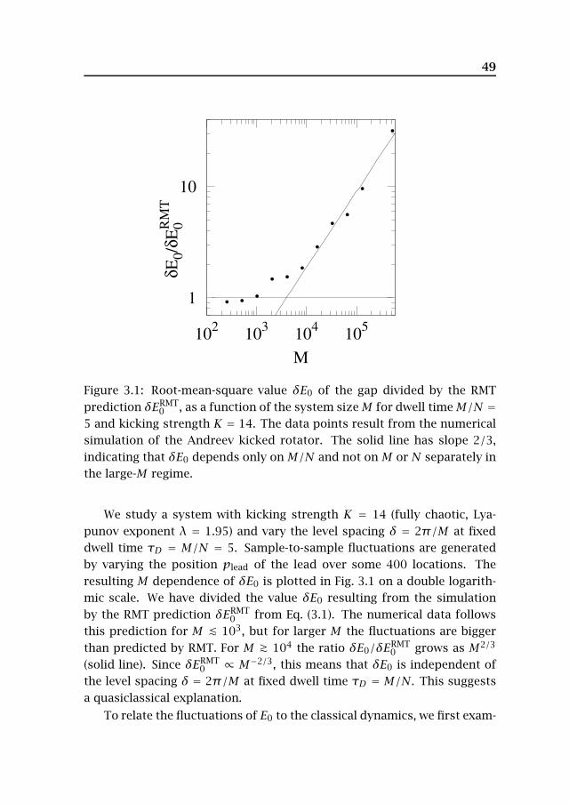
Figure 3.1: Root-mean-square value δE0 of the gap divided by the RMTprediction δERMT
0 , as a function of the system sizeM for dwell timeM/N =5 and kicking strength K = 14. The data points result from the numericalsimulation of the Andreev kicked rotator. The solid line has slope 2/3,indicating that δE0 depends only onM/N and not on M or N separately inthe large-M regime.
We study a system with kicking strength K = 14 (fully chaotic, Lya-punov exponent λ = 1.95) and vary the level spacing δ = 2π/M at fixeddwell time τD = M/N = 5. Sample-to-sample fluctuations are generatedby varying the position plead of the lead over some 400 locations. Theresulting M dependence of δE0 is plotted in Fig. 3.1 on a double logarith-mic scale. We have divided the value δE0 resulting from the simulationby the RMT prediction δERMT
0 from Eq. (3.1). The numerical data followsthis prediction for M 103, but for larger M the fluctuations are biggerthan predicted by RMT. For M 104 the ratio δE0/δERMT
0 grows as M2/3
(solid line). Since δERMT0 ∝ M−2/3, this means that δE0 is independent of
the level spacing δ = 2π/M at fixed dwell time τD = M/N. This suggestsa quasiclassical explanation.
To relate the fluctuations of E0 to the classical dynamics, we first exam-
50 Chapter 3. Quasiclassical fluctuations . . .
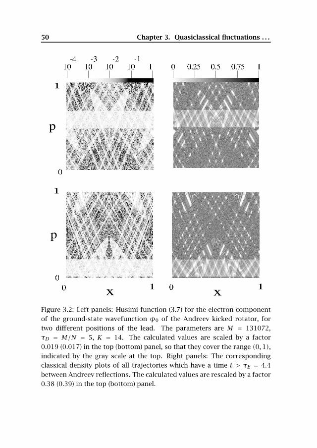
Figure 3.2: Left panels: Husimi function (3.7) for the electron componentof the ground-state wavefunction ψ0 of the Andreev kicked rotator, fortwo different positions of the lead. The parameters are M = 131072,τD = M/N = 5, K = 14. The calculated values are scaled by a factor0.019 (0.017) in the top (bottom) panel, so that they cover the range (0,1),indicated by the gray scale at the top. Right panels: The correspondingclassical density plots of all trajectories which have a time t > τE = 4.4between Andreev reflections. The calculated values are rescaled by a factor0.38 (0.39) in the top (bottom) panel.
51
ine the corresponding wavefunction ψ0. In the RMT regime the wavefunc-tions are random and show no features of the classical trajectories. In thequasiclassical regime τE τD we expect to see some classical features.Phase space portraits of the electron components ψem of the wavefunc-tions are given by the Husimi function
H (nx,np) = |〈ψem|nx,np〉|2. (3.7)
The state |nx,np〉 is a Gaussian wave packet centered at x = nx/M , p =np/M . In momentum representation it reads
〈n|nx,np〉 ∝ e−π(n−np)2/Me2πinxn/M. (3.8)
In Fig. 3.2, left panels, the Husimi function of ψ0 is shown for two leadpositions. Shown is a logarithmic gray scale density plot of the Husimifunction, with light (dark) areas corresponding to low (high) density. Thelead is visible as a light strip parallel to the x-axis. It is clear that thesewavefunctions are not random. We expect that the structure that one seescorresponds to long classical trajectories, since the wavefunctions are forthe excitation gap. To test this expectation, we show in the right panels(on a linear gray scale) the corresponding classical density plots for alltrajectories with dwell time t > τE . A total of 3 · 105 initial conditions(x0, p0) for these trajectories are chosen uniformly in the lead. Each newiteration of the map (3.6) gives a point (xn,pn) in phase space, which iskept if the time of return to the lead is greater than the Ehrenfest timeτE λ−1 ln (N2/M) = 4.4. There is a clear correspondence between thequantum mechanical Husimi function and the classical density plot. Weconclude that the wavefunction of the lowest excitation covers predomi-nantly that part of phase space where the longest dwell times occur.
To make this more quantitative we have done a quasiclassical calcula-tion, based on the effective RMT of the previous chapter. Effective RMTis valid for the part of phase space containing the long trajectories, whichhave an average time between Andreev reflections
〈T〉∗ =∫∞τETP(T)dT. (3.9)
In the pictorial representation of effective RMT (cf. Fig. 2.5), there is a longlead with delay time τE/2 and a chaotic cavity with dwell time
τD = 〈T〉∗ − τE. (3.10)
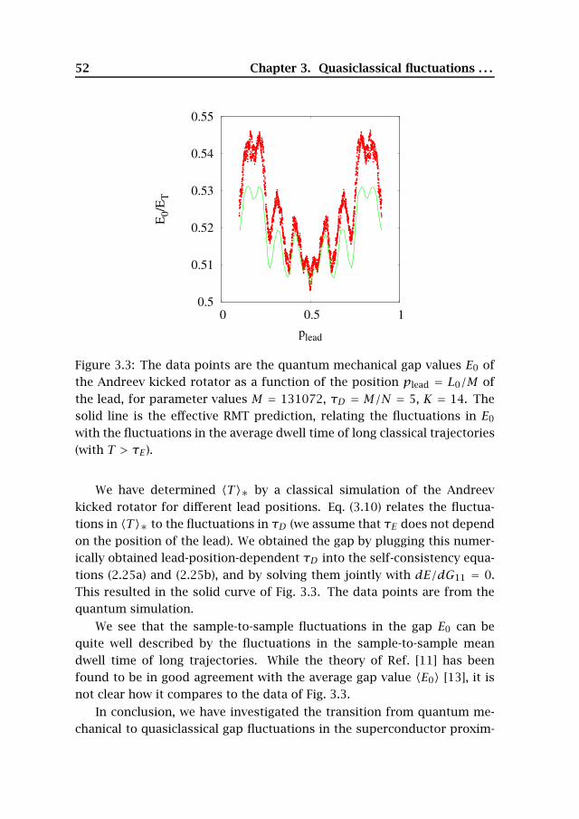
52 Chapter 3. Quasiclassical fluctuations . . .
0.5
0.51
0.52
0.53
0.54
0.55
0 0.5 1
E0/
ET
plead
Figure 3.3: The data points are the quantum mechanical gap values E0 ofthe Andreev kicked rotator as a function of the position plead = L0/M ofthe lead, for parameter values M = 131072, τD = M/N = 5, K = 14. Thesolid line is the effective RMT prediction, relating the fluctuations in E0
with the fluctuations in the average dwell time of long classical trajectories(with T > τE).
We have determined 〈T〉∗ by a classical simulation of the Andreevkicked rotator for different lead positions. Eq. (3.10) relates the fluctua-tions in 〈T〉∗ to the fluctuations in τD (we assume that τE does not dependon the position of the lead). We obtained the gap by plugging this numer-ically obtained lead-position-dependent τD into the self-consistency equa-tions (2.25a) and (2.25b), and by solving them jointly with dE/dG11 = 0.This resulted in the solid curve of Fig. 3.3. The data points are from thequantum simulation.
We see that the sample-to-sample fluctuations in the gap E0 can bequite well described by the fluctuations in the sample-to-sample meandwell time of long trajectories. While the theory of Ref. [11] has beenfound to be in good agreement with the average gap value 〈E0〉 [13], it isnot clear how it compares to the data of Fig. 3.3.
In conclusion, we have investigated the transition from quantum me-chanical to quasiclassical gap fluctuations in the superconductor proxim-

53
ity effect. The transition is accompanied by a loss of universality anda substantial enhancement of the fluctuations. Our numerical data pro-vides support for the effective random-matrix theory in a reduced partof phase space of chapter 2, as is witnessed by the relationship whichwe have found between the value of the gap and the dwell time of longclassical trajectories (see Fig. 3.3). Similar quasiclassical fluctuations ofthe conductance in a ballistic chaotic system have been found numericallyand they can also be well described by effective RMT [22].

54 Chapter 3. Quasiclassical fluctuations . . .
Bibliography
[1] Y. Imry, Introduction to Mesoscopic Physics (Oxford University, Oxford,1997).
[2] Yu.M. Galperin and V.I. Kozub, Europhys. Lett. 15, 631 (1991).
[3] B.L. Altshuler, JETP Lett. 41, 648 (1985).
[4] P.A. Lee and A.D. Stone, Phys. Rev. Lett. 55, 1622 (1985).
[5] C.W.J. Beenakker, Phys. Rev. B 47, 15763 (1993).
[6] C.W.J. Beenakker, Rev. Mod. Phys. 69, 731 (1997).
[7] T. Guhr, A. Muller-Groeling, and H. A. Weidenmuller, Phys. Rep. 299,189 (1998).
[8] Y. Alhassid, Rev. Mod. Phys. 72, 895 (2000).
[9] A. Lodder and Yu. V. Nazarov, Phys. Rev. B 58, 5783 (1998).
[10] I.L. Aleiner and A.I. Larkin, Phys. Rev. B 54, 14423 (1996).
[11] M.G. Vavilov and A.I. Larkin, Phys. Rev. B 67, 115335 (2003).
[12] G.M. Zaslavsky, Phys. Rep. 80, 157 (1981).
[13] Ph. Jacquod, H. Schomerus, and C.W.J. Beenakker, Phys. Rev. Lett. 90,207004 (2003).
[14] M.G. Vavilov, P.W. Brouwer, V. Ambegaokar, and C.W.J. Beenakker,Phys. Rev. Lett. 86, 874 (2001).
[15] F.M. Izrailev, Phys. Rep. 196, 299 (1990).
56 Bibliography
[16] R. Ketzmerick, K. Kruse, and T. Geisel, Physica D 131, 247 (1999).
[17] S. Fishman, D. R. Grempel, and R. E. Prange, Phys. Rev. Lett. 49, 509(1984).
[18] A. Altland and M. R. Zirnbauer, Phys. Rev. Lett. 77, 4536 (1996).
[19] J. Tworzydło, A. Tajic, H. Schomerus, and C.W.J. Beenakker, Phys. Rev.B, 115313 (2003).
[20] I. Adagideli and Ph. Jacquod, Phys. Rev. B 69, 020503 (2004).
[21] C. W. J. Beenakker, Lect. Notes Phys. 667, 131 (2005); cond-mat/0406018.
[22] J. Tworzydło, A. Tajic, and C. W. J. Beenakker, Phys. Rev. B 69, 165318(2004).
Chapter 4
Quantum-to-classical crossover
for Andreev billiards in a
magnetic field
4.1 Introduction
When a quantum dot is coupled to a superconductor via a point contact,the conversion of electron to hole excitations by Andreev reflection gov-erns the low-energy spectrum. The density of states of such an Andreevbilliard was calculated using random-matrix theory (RMT) [1]. If the classi-cal dynamics in the isolated quantum dot is chaotic, a gap opens up in thespectrum. The excitation gap Egap is of the order of the Thouless energy/τD , with τD the average time between Andreev reflections. Althoughchaoticity of the dynamics is essential for the gap to open, the size ofthe gap in RMT is independent of the Lyapunov exponent λ of the chaoticdynamics.
If the size L of the quantum dot is much larger than the Fermi wave-length λF , a competing timescale τE λ−1 ln (L/λF) appears, the Ehrenfesttime, which causes the breakdown of RMT [2]. The gap becomes dependenton the Lyapunov exponent and for τE τD vanishes as Egap /τE . TheEhrenfest time dependence of the gap has been investigated in chapter 2and 3 and in several other works [3–7]. For a recent review, see Ref. [8].
A magnetic field breaks time-reversal symmetry, thereby reducing Egap.At a critical field Bc the gap closes. This was calculated using RMT in Ref.
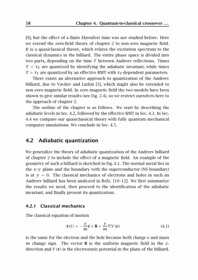
58 Chapter 4. Quantum-to-classical crossover . . .
[9], but the effect of a finite Ehrenfest time was not studied before. Herewe extend the zero-field theory of chapter 2 to non-zero magnetic field.It is a quasiclassical theory, which relates the excitation spectrum to theclassical dynamics in the billiard. The entire phase space is divided intotwo parts, depending on the time T between Andreev reflections. TimesT < τE are quantized by identifying the adiabatic invariant, while timesT > τE are quantized by an effective RMT with τE-dependent parameters.
There exists an alternative approach to quantization of the Andreevbilliard, due to Vavilov and Larkin [5], which might also be extended tonon-zero magnetic field. In zero magnetic field the two models have beenshown to give similar results (see Fig. 2.4), so we restrict ourselves here tothe approach of chapter 2.
The outline of the chapter is as follows. We start by describing theadiabatic levels in Sec. 4.2, followed by the effective RMT in Sec. 4.3. In Sec.4.4 we compare our quasiclassical theory with fully quantum mechanicalcomputer simulations. We conclude in Sec. 4.5.
4.2 Adiabatic quantization
We generalize the theory of adiabatic quantization of the Andreev billiardof chapter 2 to include the effect of a magnetic field. An example of thegeometry of such a billiard is sketched in Fig. 4.1. The normal metal lies inthe x-y plane and the boundary with the superconductor (NS boundary)is at y = 0. The classical mechanics of electrons and holes in such anAndreev billiard has been analyzed in Refs. [10–12]. We first summarizethe results we need, then proceed to the identification of the adiabaticinvariant, and finally present its quantization.
4.2.1 Classical mechanics
The classical equation of motion
r(t) = − em
r× B+ em∇V(r) (4.1)
is the same for the electron and the hole because both charge e and massm change sign. The vector B is the uniform magnetic field in the z-direction and V(r) is the electrostatic potential in the plane of the billiard.
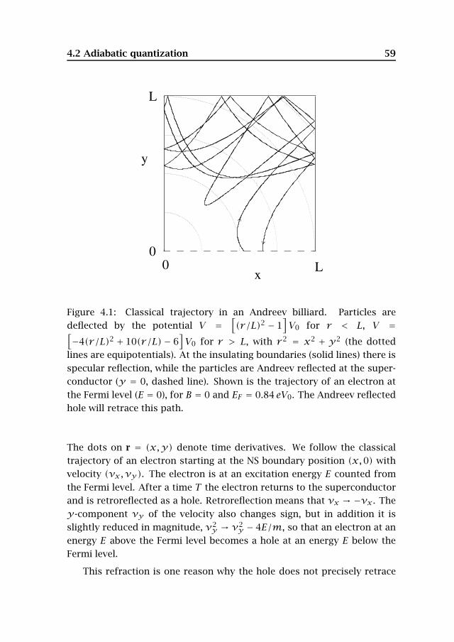
4.2 Adiabatic quantization 59
0 0
L
Lx
y
Figure 4.1: Classical trajectory in an Andreev billiard. Particles aredeflected by the potential V =
[(r/L)2 − 1
]V0 for r < L, V =[
−4(r/L)2 + 10(r/L)− 6]V0 for r > L, with r 2 = x2 + y2 (the dotted
lines are equipotentials). At the insulating boundaries (solid lines) there isspecular reflection, while the particles are Andreev reflected at the super-conductor (y = 0, dashed line). Shown is the trajectory of an electron atthe Fermi level (E = 0), for B = 0 and EF = 0.84 eV0. The Andreev reflectedhole will retrace this path.
The dots on r = (x,y) denote time derivatives. We follow the classicaltrajectory of an electron starting at the NS boundary position (x,0) withvelocity (vx, vy). The electron is at an excitation energy E counted fromthe Fermi level. After a time T the electron returns to the superconductorand is retroreflected as a hole. Retroreflection means that vx → −vx . They-component vy of the velocity also changes sign, but in addition it isslightly reduced in magnitude, v2
y → v2y − 4E/m, so that an electron at an
energy E above the Fermi level becomes a hole at an energy E below theFermi level.
This refraction is one reason why the hole does not precisely retrace
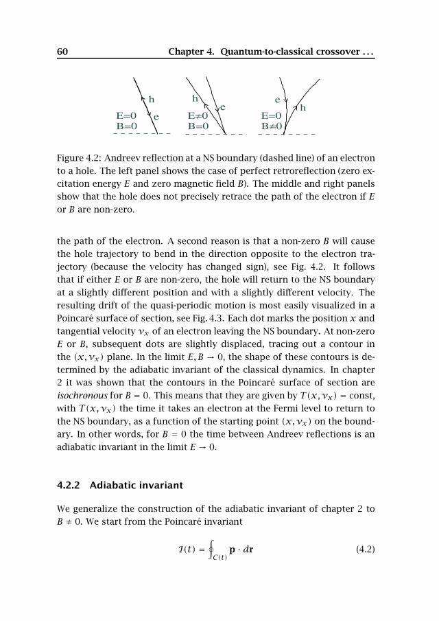
60 Chapter 4. Quantum-to-classical crossover . . .
ehe
e
hh
E=0B=0
E=0B=0
E=0B=0
Figure 4.2: Andreev reflection at a NS boundary (dashed line) of an electronto a hole. The left panel shows the case of perfect retroreflection (zero ex-citation energy E and zero magnetic field B). The middle and right panelsshow that the hole does not precisely retrace the path of the electron if Eor B are non-zero.
the path of the electron. A second reason is that a non-zero B will causethe hole trajectory to bend in the direction opposite to the electron tra-jectory (because the velocity has changed sign), see Fig. 4.2. It followsthat if either E or B are non-zero, the hole will return to the NS boundaryat a slightly different position and with a slightly different velocity. Theresulting drift of the quasi-periodic motion is most easily visualized in aPoincare surface of section, see Fig. 4.3. Each dot marks the position x andtangential velocity vx of an electron leaving the NS boundary. At non-zeroE or B, subsequent dots are slightly displaced, tracing out a contour inthe (x,vx) plane. In the limit E, B → 0, the shape of these contours is de-termined by the adiabatic invariant of the classical dynamics. In chapter2 it was shown that the contours in the Poincare surface of section areisochronous for B = 0. This means that they are given by T(x,vx) = const,with T(x,vx) the time it takes an electron at the Fermi level to return tothe NS boundary, as a function of the starting point (x,vx) on the bound-ary. In other words, for B = 0 the time between Andreev reflections is anadiabatic invariant in the limit E → 0.
4.2.2 Adiabatic invariant
We generalize the construction of the adiabatic invariant of chapter 2 toB ≠ 0. We start from the Poincare invariant
I(t) =∮C(t)
p · dr (4.2)
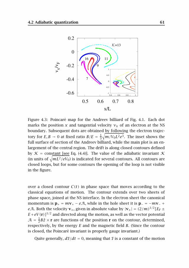
4.2 Adiabatic quantization 61
-0.6
-0.4
-0.2
0
0.2
0.5 0.6 0.7 0.8
v x/v
F
x/L
K=13
11
9
16
7
-1
-0.5
0
0.5
1
0.4 0.6 0.8 1
Figure 4.3: Poincare map for the Andreev billiard of Fig. 4.1. Each dotmarks the position x and tangential velocity vx of an electron at the NSboundary. Subsequent dots are obtained by following the electron trajec-
tory for E, B → 0 at fixed ratio B/E = 13
√m/V0L2e3. The inset shows the
full surface of section of the Andreev billiard, while the main plot is an en-largement of the central region. The drift is along closed contours definedby K = constant [see Eq. (4.4)]. The value of the adiabatic invariant K(in units of
√mL2/eV0) is indicated for several contours. All contours are
closed loops, but for some contours the opening of the loop is not visiblein the figure.
over a closed contour C(t) in phase space that moves according to theclassical equations of motion. The contour extends over two sheets ofphase space, joined at the NS interface. In the electron sheet the canonicalmomentum is p+ =mv+ − eA, while in the hole sheet it is p− = −mv− +eA. Both the velocity v±, given in absolute value by |v±| = (2/m)1/2[EF ±E+eV(r)]1/2 and directed along the motion, as well as the vector potentialA = 1
2Bz × r are functions of the position r on the contour, determined,respectively, by the energy E and the magnetic field B. (Since the contouris closed, the Poincare invariant is properly gauge invariant.)
Quite generally, dI/dt = 0, meaning that I is a constant of the motion
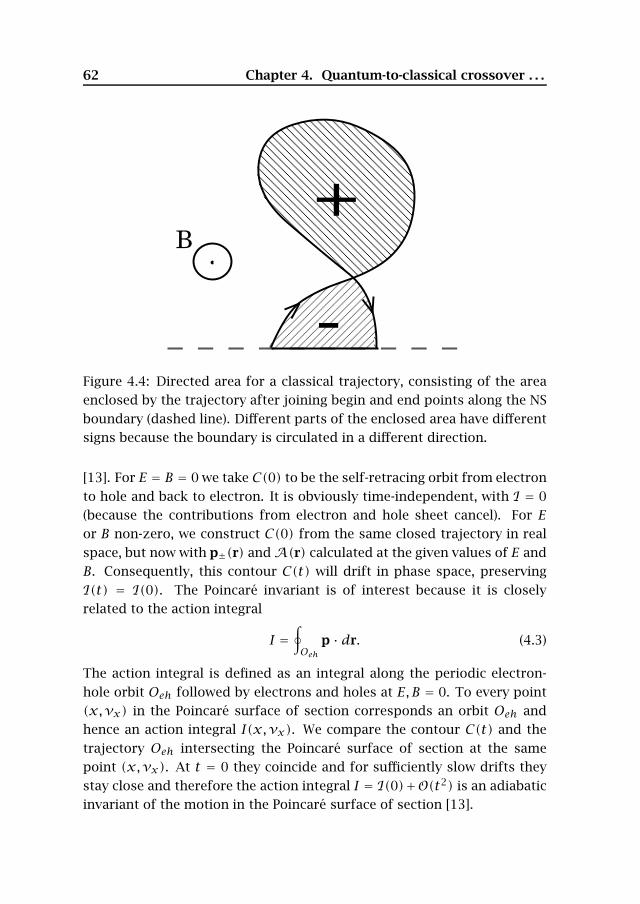
62 Chapter 4. Quantum-to-classical crossover . . .
-
+B
Figure 4.4: Directed area for a classical trajectory, consisting of the areaenclosed by the trajectory after joining begin and end points along the NSboundary (dashed line). Different parts of the enclosed area have differentsigns because the boundary is circulated in a different direction.
[13]. For E = B = 0 we take C(0) to be the self-retracing orbit from electronto hole and back to electron. It is obviously time-independent, with I = 0(because the contributions from electron and hole sheet cancel). For Eor B non-zero, we construct C(0) from the same closed trajectory in realspace, but now with p±(r) andA(r) calculated at the given values of E andB. Consequently, this contour C(t) will drift in phase space, preservingI(t) = I(0). The Poincare invariant is of interest because it is closelyrelated to the action integral
I =∮Oeh
p · dr. (4.3)
The action integral is defined as an integral along the periodic electron-hole orbit Oeh followed by electrons and holes at E, B = 0. To every point(x,vx) in the Poincare surface of section corresponds an orbit Oeh andhence an action integral I(x, vx). We compare the contour C(t) and thetrajectory Oeh intersecting the Poincare surface of section at the samepoint (x,vx). At t = 0 they coincide and for sufficiently slow drifts theystay close and therefore the action integral I = I(0)+O(t2) is an adiabaticinvariant of the motion in the Poincare surface of section [13].
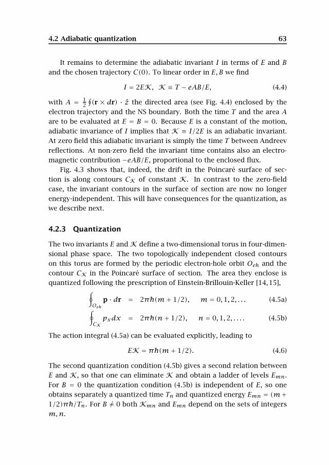
4.2 Adiabatic quantization 63
It remains to determine the adiabatic invariant I in terms of E and Band the chosen trajectory C(0). To linear order in E, B we find
I = 2EK, K ≡ T − eAB/E, (4.4)
with A = 12
∮(r × dr) · z the directed area (see Fig. 4.4) enclosed by the
electron trajectory and the NS boundary. Both the time T and the area Aare to be evaluated at E = B = 0. Because E is a constant of the motion,adiabatic invariance of I implies that K ≡ I/2E is an adiabatic invariant.At zero field this adiabatic invariant is simply the time T between Andreevreflections. At non-zero field the invariant time contains also an electro-magnetic contribution −eAB/E, proportional to the enclosed flux.
Fig. 4.3 shows that, indeed, the drift in the Poincare surface of sec-tion is along contours CK of constant K. In contrast to the zero-fieldcase, the invariant contours in the surface of section are now no longerenergy-independent. This will have consequences for the quantization, aswe describe next.
4.2.3 Quantization
The two invariants E andK define a two-dimensional torus in four-dimen-sional phase space. The two topologically independent closed contourson this torus are formed by the periodic electron-hole orbit Oeh and thecontour CK in the Poincare surface of section. The area they enclose isquantized following the prescription of Einstein-Brillouin-Keller [14,15],∮
Oehp · dr = 2π(m+ 1/2), m = 0,1,2, . . . (4.5a)
∮CKpxdx = 2π(n+ 1/2), n = 0,1,2, . . . . (4.5b)
The action integral (4.5a) can be evaluated explicitly, leading to
EK = π(m+ 1/2). (4.6)
The second quantization condition (4.5b) gives a second relation betweenE and K, so that one can eliminate K and obtain a ladder of levels Emn.For B = 0 the quantization condition (4.5b) is independent of E, so oneobtains separately a quantized time Tn and quantized energy Emn = (m+1/2)π/Tn. For B = 0 both Kmn and Emn depend on the sets of integersm,n.
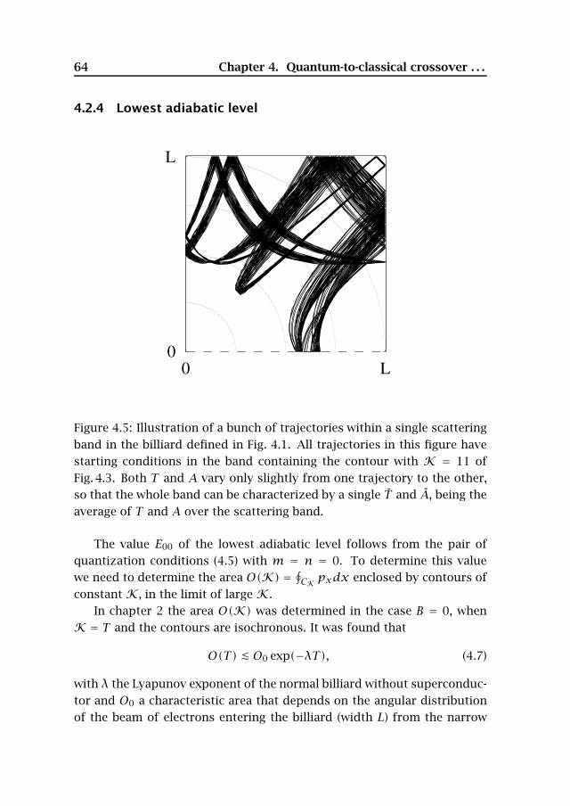
64 Chapter 4. Quantum-to-classical crossover . . .
4.2.4 Lowest adiabatic level
L
0L0
Figure 4.5: Illustration of a bunch of trajectories within a single scatteringband in the billiard defined in Fig. 4.1. All trajectories in this figure havestarting conditions in the band containing the contour with K = 11 ofFig. 4.3. Both T and A vary only slightly from one trajectory to the other,so that the whole band can be characterized by a single T and A, being theaverage of T and A over the scattering band.
The value E00 of the lowest adiabatic level follows from the pair ofquantization conditions (4.5) with m = n = 0. To determine this valuewe need to determine the area O(K) = ∮CK pxdx enclosed by contours ofconstant K, in the limit of large K.
In chapter 2 the area O(K) was determined in the case B = 0, whenK = T and the contours are isochronous. It was found that
O(T) O0 exp(−λT), (4.7)
with λ the Lyapunov exponent of the normal billiard without superconduc-tor and O0 a characteristic area that depends on the angular distributionof the beam of electrons entering the billiard (width L) from the narrow
4.2 Adiabatic quantization 65
contact to the superconductor (width W ). For a collimated beam having aspread of velocities |vW/vF | W/L one has O0 = Nh (see chapter 2). Fora non-collimated beam O0 = NhW/L (this will be explained in chapter 5).The integer N is the number of scattering channels connecting the billiardto the superconductor. The quantization requirement O(T) ≥ π givesthe lowest adiabatic level in zero magnetic field,
E00(B = 0) = π2τE
, τE = 1λ[ln (O0/π)+O(1)] . (4.8)
The Ehrenfest time τE corresponds to a contour that encloses an area π.In order to generalize Eq. (4.7) to B = 0, we discuss the concept of
scattering bands, which will be discussed in chapter 5 for a normal bil-liard (where they are called transmission and reflection bands). Scatteringbands are ordered phase space structures that appear in open systems,even if their closed counterparts are fully chaotic. These structures arecharacterized by regions in which the functions T(x,vx) and A(x,vx)vary slowly almost everywhere. Hence, they contain orbits of almost con-stant return time and directed area, that is, orbits returning by bunches.One such bunch is depicted in Fig. 4.5. The scattering bands are boundedby contours of diverging T(x,vx) and A(x,vx). The divergence is veryslow (∝ 1/ ln ε, with ε the distance from the contour [4]), so the mean re-turn time T and mean directed area A in a scattering band remain finiteand well defined [16].
The area Oband of a band depends on T as (see chapter 5)
Oband(T ) O0 exp (−λT ). (4.9)
Since an isochronous contour must lie within a single scattering band,Eq. (4.7) follows from Eq. (4.9) and from the fact that the distribution ofreturn times is sharply peaked around the mean T . Because contours ofconstant K = T − eAB/E must also lie within a single scattering band, thearea O(K) is bounded by the same function Oband(T ). We conclude thatwithin a given scattering band the largest contour of constant T and thelargest contour of constant K each have approximately the same area asthe band itself,
O(T),O(K) Oband(T ) O0 exp(−λT). (4.10)
We are now ready to determine the magnetic field dependence of thelowest adiabatic level E00(B). The corresponding contour CK lies in a
66 Chapter 4. Quantum-to-classical crossover . . .
band characterized by a mean return time T λ−1 ln (O0/π), accordingto Eqs. (4.5b) and (4.10). This is the same Ehrenfest time as Eq. (4.8)for B = 0 (assuming that the orbital effect of the magnetic field does notmodify λ) . The energy of the lowest adiabatic level E00 is determined bythe quantization condition (4.6),
E00K E00τE + eAmaxB = π/2. (4.11)
The range of directed areas −Amax A Amax is the product of the areaL2 of the billiard and the maximum number of times nmax ≈ vFT /L that atrajectory can encircle that area (clockwise or counterclockwise) in a timeT . Hence Amax = vF TL vFτEL and we find
E00(B) ≡ Eadgap
π2τE
− evFLB. (4.12)
We conclude that a magnetic field shifts the lowest adiabatic leveldownward by an amount evFLB which is independent of τE . Eq. (4.12)holds up to a field Bad
c at which the lowest adiabatic level reaches theFermi level,
Badc π
2eAmax π
2τEevFL. (4.13)
We have added the label “ad”, because the true critical field at which thegap closes may be smaller due to non-adiabatic levels below E00. For B = 0,the ground state is never an adiabatic state (chapter 2). In the next sectionwe study the effective RMT, in order to determine the contribution fromnon-adiabatic levels (return times T > τE).
4.2.5 Density of states
The pair of quantization conditions (4.5) determines the individual energylevels with T < τE and |A| < Amax vFτEL. For semiclassical systemswith L/λF 1 the level spacing δ of the isolated billiard is so small thatindividual levels are not resolved and it suffices to know the smoothed (orensemble averaged) density of states ρad(E). In view of Eq. (4.6) it is givenby
ρad(E) = N∫ τE
0dT∫ Amax
−Amax
dAP(T ,A)×∑mδ(E − π(m + 1/2)+ eAB
T
),
(4.14)
4.3 Effective random-matrix theory 67
in terms of the joint distribution function P(T ,A) of return time T anddirected area A. In the limit τE → ∞ this formula reduces to the Bohr-Sommerfeld quantization rule of Ref. [1] for B = 0 and to the generaliza-tion of Ref. [17] for B = 0. The adiabatic density of states (4.14) vanishesfor E < Ead
gap. Its high energy asymptotics (meaning E Eadgap, but still
E ∆) can be estimated using P(T ,A) = P(A|T)P(T) with the condi-tional distribution P(A|T) (which will be discussed in the next section)and the return time distribution P(T) = exp (−T/τD)τ−1
D . One gets
limE→∞E∆
ρad(E) =2δ
(1− e−τE/τD
[1+ τE
τD
]). (4.15)
The limit (4.15) is less than the value 2/δ, which also contains the contri-bution from the non-adiabatic levels with T > τE .
4.3 Effective random-matrix theory
The adiabatic quantization applies only to the part of phase space in whichthe return time T is less than the Ehrenfest time τE . To quantize the re-mainder, with T > τE , we apply the effective random-matrix theory (RMT)of chapter 2. The existing formulation does not yet include a magneticfield, so we begin by extending it to non-zero B.
4.3.1 Effective cavity
The effective RMT is based on the decomposition of the scattering matrixin the time domain into two parts,
S(t) =Scl(t) if t < τESq(t) if t > τE .
(4.16)
The classical, short-time part Scl(t) couples to Ncl scattering channels ofreturn time < τE , which can be quantized adiabatically as explained in theprevious section. The remaining
Nq = N −Ncl = Ne−τE/τD ≡ Neff (4.17)
quantum channels, with return time > τE , are quantized by RMT witheffective τE-dependent parameters.
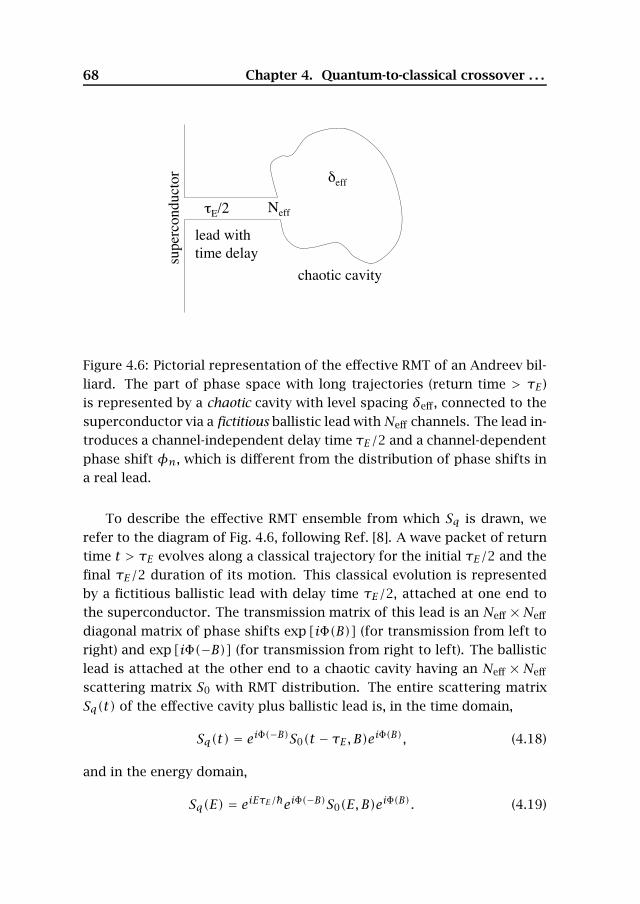
68 Chapter 4. Quantum-to-classical crossover . . .
Figure 4.6: Pictorial representation of the effective RMT of an Andreev bil-liard. The part of phase space with long trajectories (return time > τE )is represented by a chaotic cavity with level spacing δeff, connected to thesuperconductor via a fictitious ballistic lead withNeff channels. The lead in-troduces a channel-independent delay time τE/2 and a channel-dependentphase shift φn, which is different from the distribution of phase shifts ina real lead.
To describe the effective RMT ensemble from which Sq is drawn, werefer to the diagram of Fig. 4.6, following Ref. [8]. A wave packet of returntime t > τE evolves along a classical trajectory for the initial τE/2 and thefinal τE/2 duration of its motion. This classical evolution is representedby a fictitious ballistic lead with delay time τE/2, attached at one end tothe superconductor. The transmission matrix of this lead is an Neff ×Neff
diagonal matrix of phase shifts exp [iΦ(B)] (for transmission from left toright) and exp [iΦ(−B)] (for transmission from right to left). The ballisticlead is attached at the other end to a chaotic cavity having an Neff × Neff
scattering matrix S0 with RMT distribution. The entire scattering matrixSq(t) of the effective cavity plus ballistic lead is, in the time domain,
Sq(t) = eiΦ(−B)S0(t − τE, B)eiΦ(B), (4.18)
and in the energy domain,
Sq(E) = eiEτE/eiΦ(−B)S0(E, B)eiΦ(B). (4.19)
4.3 Effective random-matrix theory 69
The level spacing δeff of the effective cavity is increased according to
δeff/δ = N/Neff = eτE/τD , (4.20)
to ensure that the mean dwell time 2π/Neffδeff remains equal to τD , in-dependent of the Ehrenfest time.
For weak magnetic fields (such that the cyclotron radiusmvF/eB L),the phase shifts Φ(B) are linear in B:
Φ(B) Φ(0)+ BΦ′(0) ≡ Φ(0)+ diag[φ1,φ2 . . .φNeff
]. (4.21)
The phases φn are the channel-dependent, magnetic field induced phaseshifts of classical trajectories spending a time τE/2 in a chaotic cavity.
The conditional distribution of directed areas A for a given return timeT is a truncated Gaussian [17,18],
P(A|T) ∝ exp(−A2/A2
0
)θ(Amax − |A|),
A20 ∝ vFTL3, (4.22)
with θ(x) the unit step function. This implies that the distribution P(φ)of phase shifts φ = eAB/ for T = τE/2 is given by
P(φ) ∝ exp
[−φ
2
cτDτE
(B0
B
)2]θ (φmax − |φ|) , (4.23)
φmax = eAmaxB
BB0
√√√√vFτ2E
LτD. (4.24)
The constant c of order unity is determined by the billiard geometry andB0 denotes the critical magnetic field of the Andreev billiard when τE → 0.Up to numerical coefficients of order unity, one has [9]
B0 eL2
√L
vFτD. (4.25)
4.3.2 Density of states
The energy spectrum of an Andreev billiard, for energies well below thegap ∆ of the bulk superconductor, is related to the scattering matrix bythe determinantal equation [19]
70 Chapter 4. Quantum-to-classical crossover . . .
Det[1+ S(E)S∗(−E)] = 0. (4.26)
Since Scl and Sq couple to different channels, we may calculate separatelythe contribution to the spectrum from the effective cavity, governed by Sq.We substitute the expression (4.19) for Sq, to obtain
Det[1+ e2iEτE/S0(E, B)Ω(B)S∗0 (−E, B)Ω∗(B)
]= 0, (4.27)
Ω(B) ≡ eiΦ(B)−iΦ(−B) = diag[e2iφ1 , e2iφ2 . . . e2iφNeff ]. (4.28)
In chapter 2 the density of states was calculated from this equation forthe case B = 0, when Ω = 1. We generalize the calculation to B = 0. Thetechnicalities are very similar to those of Ref. [20].
The scattering matrix S0(E, B) of the open effective cavity can be rep-resented by [21,22]
S0(E, B) = 1− 2πiWT[E −H0(B)+ iπWWT
]−1W, (4.29)
in terms of the Hamiltonian H0(B) of the closed effective cavity and acoupling matrix W . The dimension of H0 is M × M and the dimensionof W is M × Neff. The matrix WTW has eigenvalues Mδeff/π2. The limitM → ∞ at fixed level spacing δeff is taken at the end of the calculation.Substitution of Eq. (4.29) into the determinantal equation (4.27) gives aconventional eigenvalue equation [20],
Det [E −Heff(B)] = 0, (4.30)
Heff(B) =(H0(B) 0
0 −H∗0 (B)
)−W , (4.31)
W = πcosu
(WWT sinu WΩ(B)WT
WΩ∗(B)WT WWT sinu
). (4.32)
We have abbreviated u = EτE/.The Hamiltonian H0(B) of the fictitious cavity has the Pandey-Mehta
distribution [23],
P(H) ∝ exp
⎛⎝−π2(1+ b2)
4Mδ2eff
M∑i,j=1
[(ReHij)2 + b−2(ImHij)2
]⎞⎠ . (4.33)
4.3 Effective random-matrix theory 71
The parameter b ∈ [0,1] measures the strength of the time-reversal sym-metry breaking. It is related to the magnetic field by [9]
MNeff
b2 = 18(B/B0)2. (4.34)
The ensemble averaged density of states ρeff(E) is obtained from theGreen function,
ρeff(E) = − 1π
ImTr(
1+ dWdE
)G(E + i0+), (4.35)
G(z) = 〈(z −Heff)−1〉, (4.36)
where the average 〈· · · 〉 is taken with the distribution (4.33). Using theresults of Refs. [9, 20] we obtain a self-consistency equation for the traceof the ensemble averaged Green function,
G =(G11 G12
G21 G22
)= δπ
(TrG11 TrG12
TrG21 TrG22
). (4.37)
The four blocks refer to the block decomposition (4.31) of the effectiveHamiltonian. The self-consistency equation reads
G11 = G22, G12G21 = 1+G211, (4.38)
0 = Neff
(E
2ET−( BB0
)2 G11
2
)G12
+Neff∑j=1
e2iφjG11 +G12 sinu12
[e−2iφjG12 + e2iφjG21
]+ cosu+G11 sinu
, (4.39)
0 = Neff
(E
2ET−(BB0
)2 G11
2
)G21
+Neff∑j=1
e−2iφjG11 +G21 sinu12
[e−2iφjG12 + e2iφjG21
]+ cosu+G11 sinu
, (4.40)
with the Thouless energy ET = /2τD .From Eq. (4.35) we find the density of states
ρeff(E) = − 2δeff
Im[G11 + τE
τD cosu
×Neff∑j=1
G11 + 12 sinu
(G21e2iφj +G12e−2iφj
)cosu+G11 sinu+ 1
2G12e−2iφj + 12G21e2iφj
]. (4.41)
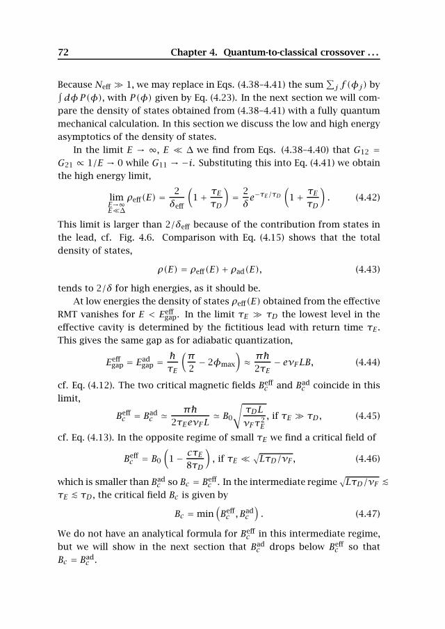
72 Chapter 4. Quantum-to-classical crossover . . .
Because Neff 1, we may replace in Eqs. (4.38–4.41) the sum∑j f (φj) by∫
dφP(φ), with P(φ) given by Eq. (4.23). In the next section we will com-pare the density of states obtained from (4.38–4.41) with a fully quantummechanical calculation. In this section we discuss the low and high energyasymptotics of the density of states.
In the limit E → ∞, E ∆ we find from Eqs. (4.38–4.40) that G12 =G21 ∝ 1/E → 0 while G11 → −i. Substituting this into Eq. (4.41) we obtainthe high energy limit,
limE→∞E∆
ρeff(E) =2δeff
(1+ τE
τD
)= 2δe−τE/τD
(1+ τE
τD
). (4.42)
This limit is larger than 2/δeff because of the contribution from states inthe lead, cf. Fig. 4.6. Comparison with Eq. (4.15) shows that the totaldensity of states,
ρ(E) = ρeff(E)+ ρad(E), (4.43)
tends to 2/δ for high energies, as it should be.At low energies the density of states ρeff(E) obtained from the effective
RMT vanishes for E < Eeffgap. In the limit τE τD the lowest level in the
effective cavity is determined by the fictitious lead with return time τE .This gives the same gap as for adiabatic quantization,
Eeffgap = Ead
gap =τE
(π2− 2φmax
)≈ π
2τE− evFLB, (4.44)
cf. Eq. (4.12). The two critical magnetic fields Beffc and Bad
c coincide in thislimit,
Beffc = Bad
c π2τEevFL
B0
√τDLvFτ2
E, if τE τD, (4.45)
cf. Eq. (4.13). In the opposite regime of small τE we find a critical field of
Beffc = B0
(1− cτE
8τD
), if τE
√LτD/vF , (4.46)
which is smaller than Badc so Bc = Beff
c . In the intermediate regime√LτD/vF
τE τD , the critical field Bc is given by
Bc = min(Beffc , Bad
c
). (4.47)
We do not have an analytical formula for Beffc in this intermediate regime,
but we will show in the next section that Badc drops below Beff
c so thatBc = Bad
c .
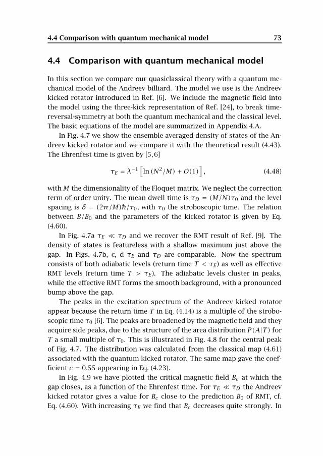
4.4 Comparison with quantum mechanical model 73
4.4 Comparison with quantum mechanical model
In this section we compare our quasiclassical theory with a quantum me-chanical model of the Andreev billiard. The model we use is the Andreevkicked rotator introduced in Ref. [6]. We include the magnetic field intothe model using the three-kick representation of Ref. [24], to break time-reversal-symmetry at both the quantum mechanical and the classical level.The basic equations of the model are summarized in Appendix 4.A.
In Fig. 4.7 we show the ensemble averaged density of states of the An-dreev kicked rotator and we compare it with the theoretical result (4.43).The Ehrenfest time is given by [5,6]
τE = λ−1[ln (N2/M)+O(1)
], (4.48)
withM the dimensionality of the Floquet matrix. We neglect the correctionterm of order unity. The mean dwell time is τD = (M/N)τ0 and the levelspacing is δ = (2π/M)/τ0, with τ0 the stroboscopic time. The relationbetween B/B0 and the parameters of the kicked rotator is given by Eq.(4.60).
In Fig. 4.7a τE τD and we recover the RMT result of Ref. [9]. Thedensity of states is featureless with a shallow maximum just above thegap. In Figs. 4.7b, c, d τE and τD are comparable. Now the spectrumconsists of both adiabatic levels (return time T < τE) as well as effectiveRMT levels (return time T > τE). The adiabatic levels cluster in peaks,while the effective RMT forms the smooth background, with a pronouncedbump above the gap.
The peaks in the excitation spectrum of the Andreev kicked rotatorappear because the return time T in Eq. (4.14) is a multiple of the strobo-scopic time τ0 [6]. The peaks are broadened by the magnetic field and theyacquire side peaks, due to the structure of the area distribution P(A|T) forT a small multiple of τ0. This is illustrated in Fig. 4.8 for the central peakof Fig. 4.7. The distribution was calculated from the classical map (4.61)associated with the quantum kicked rotator. The same map gave the coef-ficient c = 0.55 appearing in Eq. (4.23).
In Fig. 4.9 we have plotted the critical magnetic field Bc at which thegap closes, as a function of the Ehrenfest time. For τE τD the Andreevkicked rotator gives a value for Bc close to the prediction B0 of RMT, cf.Eq. (4.60). With increasing τE we find that Bc decreases quite strongly. In
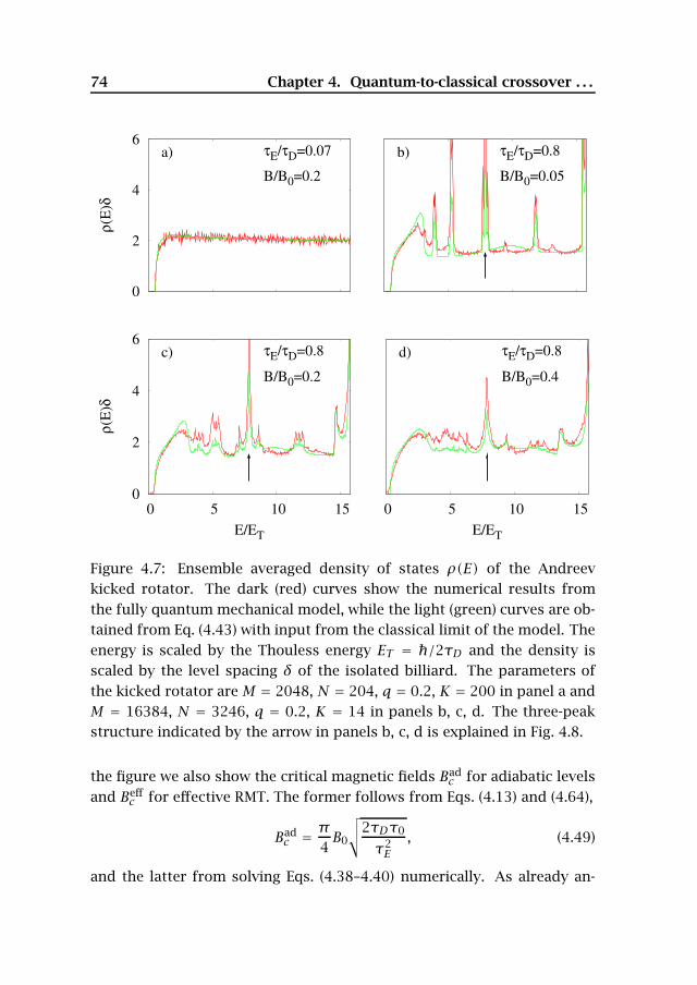
74 Chapter 4. Quantum-to-classical crossover . . .
0 5 10 15
E/ET
τE/τD=0.8
B/B0=0.4
d)
0
2
4
6
0 5 10 15
ρ(E
)δ
E/ET
τE/τD=0.8
B/B0=0.2
c)
0
2
4
6
ρ(E
)δ
τE/τD=0.07
B/B0=0.2
a) τE/τD=0.8
B/B0=0.05
b)
Figure 4.7: Ensemble averaged density of states ρ(E) of the Andreevkicked rotator. The dark (red) curves show the numerical results fromthe fully quantum mechanical model, while the light (green) curves are ob-tained from Eq. (4.43) with input from the classical limit of the model. Theenergy is scaled by the Thouless energy ET = /2τD and the density isscaled by the level spacing δ of the isolated billiard. The parameters ofthe kicked rotator are M = 2048, N = 204, q = 0.2, K = 200 in panel a andM = 16384, N = 3246, q = 0.2, K = 14 in panels b, c, d. The three-peakstructure indicated by the arrow in panels b, c, d is explained in Fig. 4.8.
the figure we also show the critical magnetic fields Badc for adiabatic levels
and Beffc for effective RMT. The former follows from Eqs. (4.13) and (4.64),
Badc = π
4B0
√√√2τDτ0
τ2E, (4.49)
and the latter from solving Eqs. (4.38–4.40) numerically. As already an-
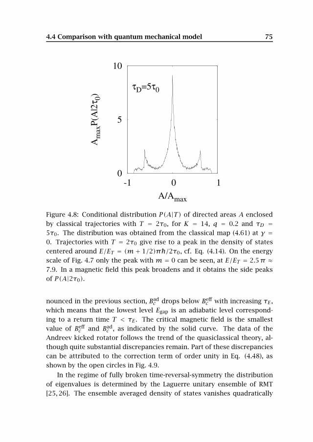
4.4 Comparison with quantum mechanical model 75
0
5
10
-1 0 1
Am
axP(
A|2
τ 0)
A/Amax
τD=5τ0
Figure 4.8: Conditional distribution P(A|T) of directed areas A enclosedby classical trajectories with T = 2τ0, for K = 14, q = 0.2 and τD =5τ0. The distribution was obtained from the classical map (4.61) at γ =0. Trajectories with T = 2τ0 give rise to a peak in the density of statescentered around E/ET = (m + 1/2)π/2τ0, cf. Eq. (4.14). On the energyscale of Fig. 4.7 only the peak with m = 0 can be seen, at E/ET = 2.5π ≈7.9. In a magnetic field this peak broadens and it obtains the side peaksof P(A|2τ0).
nounced in the previous section, Badc drops below Beff
c with increasing τE ,which means that the lowest level Egap is an adiabatic level correspond-ing to a return time T < τE . The critical magnetic field is the smallestvalue of Beff
c and Badc , as indicated by the solid curve. The data of the
Andreev kicked rotator follows the trend of the quasiclassical theory, al-though quite substantial discrepancies remain. Part of these discrepanciescan be attributed to the correction term of order unity in Eq. (4.48), asshown by the open circles in Fig. 4.9.
In the regime of fully broken time-reversal-symmetry the distributionof eigenvalues is determined by the Laguerre unitary ensemble of RMT[25, 26]. The ensemble averaged density of states vanishes quadratically
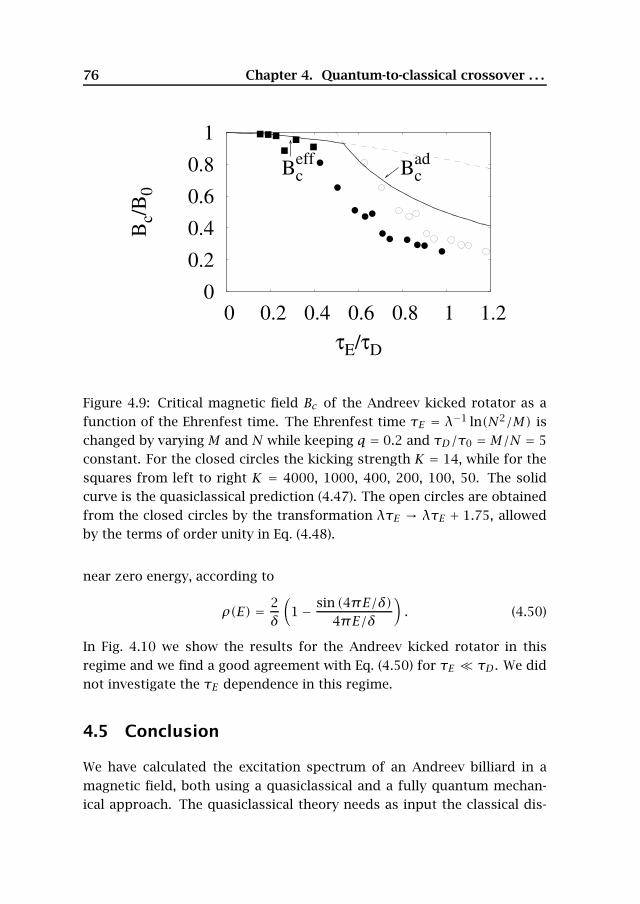
76 Chapter 4. Quantum-to-classical crossover . . .
0
0.2
0.4
0.6
0.8
1
0 0.2 0.4 0.6 0.8 1 1.2
Bc/
B0
τE/τD
BcadBc
eff
Figure 4.9: Critical magnetic field Bc of the Andreev kicked rotator as afunction of the Ehrenfest time. The Ehrenfest time τE = λ−1 ln(N2/M) ischanged by varying M and N while keeping q = 0.2 and τD/τ0 = M/N = 5constant. For the closed circles the kicking strength K = 14, while for thesquares from left to right K = 4000, 1000, 400, 200, 100, 50. The solidcurve is the quasiclassical prediction (4.47). The open circles are obtainedfrom the closed circles by the transformation λτE → λτE + 1.75, allowedby the terms of order unity in Eq. (4.48).
near zero energy, according to
ρ(E) = 2δ
(1− sin (4πE/δ)
4πE/δ
). (4.50)
In Fig. 4.10 we show the results for the Andreev kicked rotator in thisregime and we find a good agreement with Eq. (4.50) for τE τD . We didnot investigate the τE dependence in this regime.
4.5 Conclusion
We have calculated the excitation spectrum of an Andreev billiard in amagnetic field, both using a quasiclassical and a fully quantum mechan-ical approach. The quasiclassical theory needs as input the classical dis-
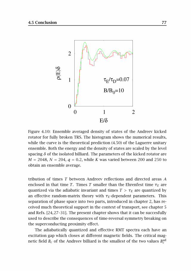
4.5 Conclusion 77
0
1
2
0 1 2
ρ(E
)δ
E/δ
τE/τD=0.07
B/B0=10
Figure 4.10: Ensemble averaged density of states of the Andreev kickedrotator for fully broken TRS. The histogram shows the numerical results,while the curve is the theoretical prediction (4.50) of the Laguerre unitaryensemble. Both the energy and the density of states are scaled by the levelspacing δ of the isolated billiard. The parameters of the kicked rotator areM = 2048, N = 204, q = 0.2, while K was varied between 200 and 250 toobtain an ensemble average.
tribution of times T between Andreev reflections and directed areas Aenclosed in that time T . Times T smaller than the Ehrenfest time τE arequantized via the adiabatic invariant and times T > τE are quantized byan effective random-matrix theory with τE-dependent parameters. Thisseparation of phase space into two parts, introduced in chapter 2, has re-ceived much theoretical support in the context of transport, see chapter 5and Refs. [24,27–31]. The present chapter shows that it can be succesfullyused to describe the consequences of time-reversal symmetry breaking onthe superconducting proximity effect.
The adiabatically quantized and effective RMT spectra each have anexcitation gap which closes at different magnetic fields. The critical mag-netic field Bc of the Andreev billiard is the smallest of the two values Bad
c
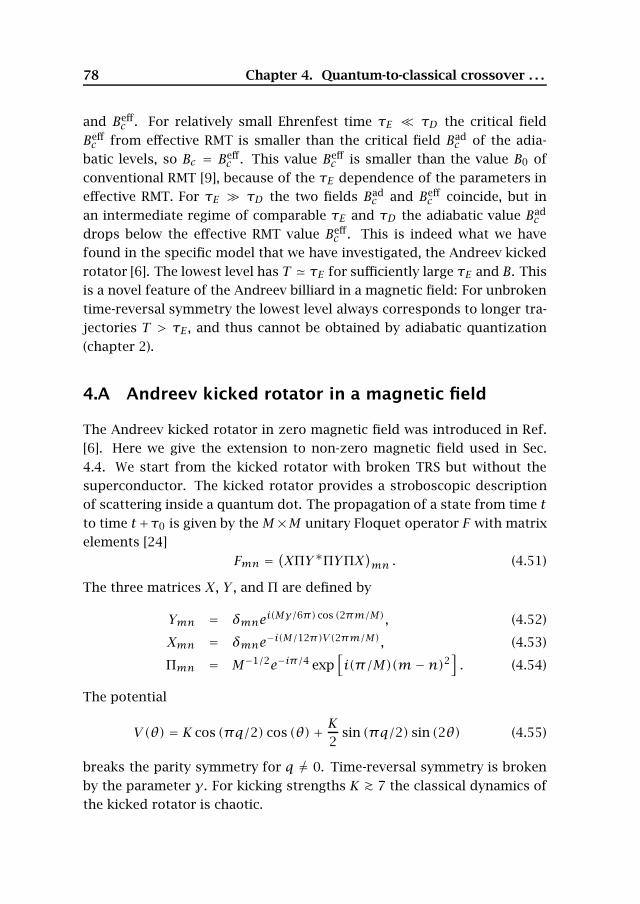
78 Chapter 4. Quantum-to-classical crossover . . .
and Beffc . For relatively small Ehrenfest time τE τD the critical field
Beffc from effective RMT is smaller than the critical field Bad
c of the adia-batic levels, so Bc = Beff
c . This value Beffc is smaller than the value B0 of
conventional RMT [9], because of the τE dependence of the parameters ineffective RMT. For τE τD the two fields Bad
c and Beffc coincide, but in
an intermediate regime of comparable τE and τD the adiabatic value Badc
drops below the effective RMT value Beffc . This is indeed what we have
found in the specific model that we have investigated, the Andreev kickedrotator [6]. The lowest level has T τE for sufficiently large τE and B. Thisis a novel feature of the Andreev billiard in a magnetic field: For unbrokentime-reversal symmetry the lowest level always corresponds to longer tra-jectories T > τE , and thus cannot be obtained by adiabatic quantization(chapter 2).
4.A Andreev kicked rotator in a magnetic field
The Andreev kicked rotator in zero magnetic field was introduced in Ref.[6]. Here we give the extension to non-zero magnetic field used in Sec.4.4. We start from the kicked rotator with broken TRS but without thesuperconductor. The kicked rotator provides a stroboscopic descriptionof scattering inside a quantum dot. The propagation of a state from time tto time t+τ0 is given by theM×M unitary Floquet operator F with matrixelements [24]
Fmn =(XΠY∗ΠYΠX
)mn . (4.51)
The three matrices X, Y , and Π are defined by
Ymn = δmnei(Mγ/6π) cos (2πm/M), (4.52)
Xmn = δmne−i(M/12π)V(2πm/M), (4.53)
Πmn = M−1/2e−iπ/4 exp[i(π/M)(m −n)2
]. (4.54)
The potential
V(θ) = K cos (πq/2) cos (θ)+ K2
sin (πq/2) sin (2θ) (4.55)
breaks the parity symmetry for q = 0. Time-reversal symmetry is brokenby the parameter γ. For kicking strengths K 7 the classical dynamics ofthe kicked rotator is chaotic.
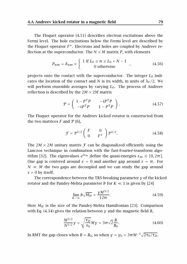
4.A Andreev kicked rotator in a magnetic field 79
The Floquet operator (4.51) describes electron excitations above theFermi level. The hole excitations below the Fermi level are described bythe Floquet operator F∗. Electrons and holes are coupled by Andreev re-flection at the superconductor. The N ×M matrix P , with elements
Pnm = δnm ×
1 if L0 ≤ n ≤ L0 +N − 10 otherwise
, (4.56)
projects onto the contact with the superconductor. The integer L0 indi-cates the location of the contact and N is its width, in units of λF/2. Wewill perform ensemble averages by varying L0. The process of Andreevreflection is described by the 2M × 2M matrix
P =(
1− PTP −iPTP−iPTP 1− PTP
). (4.57)
The Floquet operator for the Andreev kicked rotator is constructed fromthe two matrices F and P [6],
F = P1/2(F 00 F∗
)P1/2. (4.58)
The 2M × 2M unitary matrix F can be diagonalized efficiently using theLanczos technique in combination with the fast-Fourier-transform algo-rithm [32]. The eigenvalues eiεm define the quasi-energies εm ∈ [0,2π].One gap is centered around ε = 0 and another gap around ε = π . ForN M the two gaps are decoupled and we can study the gap aroundε = 0 by itself.
The correspondence between the TRS-breaking parameter γ of the kickedrotator and the Pandey-Mehta parameter b for K 1 is given by [24]
limK→∞
b√MH = γM
3/2
12π. (4.59)
Here MH is the size of the Pandey-Mehta Hamiltonian [23]. Comparisonwith Eq. (4.34) gives the relation between γ and the magnetic field B,
M3/2
N1/2 γ =√τDτ0Mγ = 3π
√2BB0. (4.60)
In RMT the gap closes when B = B0, so when γ = γ0 = 3πM−1√
2τ0/τD .
80 Chapter 4. Quantum-to-classical crossover . . .
For the quasiclassical theory we need the classical map associated withthe Floquet operator (4.58). The classical phase space consists of the torus0 ≤ θ ≤ 2π , 0 ≤ p ≤ 6π . The classical map is described by a set ofequations that map initial coordinates (θ,p) onto final coordinates (θ′, p′)after one period τ0 [24],
θ1 = θ ± p/3− V ′(θ)/6− 2πσθ1 ,
p1 = p ∓ γ sin (θ1)∓ V ′(θ)/2− 6πσp1 ,
θ2 = θ1 ± p1/3− 2πσθ2 ,
p2 = p1 − 6πσp2 ,
θ′ = θ2 ± p2/3+ γ sin (θ2)/3− 2πσθ′ ,
p′ = p2 ± γ sin(θ2)∓ V ′(θ′)/2− 6πσ ′p. (4.61)
The upper/lower signs correspond to electron/hole dynamics and V ′(θ) =dV/dθ. The integers σθ and σp are the winding numbers of a trajectoryon the torus.
The directed area enclosed by a classical trajectory between Andreevreflections can be calculated from the difference in classical action be-tween two trajectories related by TRS, one with γ = 0 and one with in-finitesimal γ. To linear order in γ the action difference ∆S acquired afterone period is given by [24]
∆S = γ (cosθ1 − cosθ2) . (4.62)
The effective Planck constant of the kicked rotator is eff = 6π/M , so wemay obtain the increment in directed area ∆A corresponding to ∆S from
eB∆A = ∆S
eff= M
6πγ (cosθ1 − cosθ2) . (4.63)
Since | cosθ1−cosθ2| < 2, the maximum directed area Amax acquired afterT/τ0 periods is
Amax = 2Tτ0
eB0
√τ0
2τD. (4.64)
Bibliography
[1] J. A. Melsen, P. W. Brouwer, K. M. Frahm, and C. W. J. Beenakker,Europhys. Lett. 35, 7 (1996).
[2] A. Lodder and Yu. V. Nazarov, Phys. Rev. B 58, 5783 (1998).
[3] D. Taras-Semchuk and A. Altland, Phys. Rev. B 64, 014512 (2001).
[4] I. Adagideli and C. W. J. Beenakker, Phys. Rev. Lett. 89, 237002 (2002).
[5] M. G. Vavilov and A. I. Larkin, Phys. Rev. B 67, 115335 (2003).
[6] Ph. Jacquod, H. Schomerus, and C. W. J. Beenakker, Phys. Rev. Lett.90, 207004 (2003).
[7] A. Kormanyos, Z. Kaufmann, C. J. Lambert, and J. Cserti, Phys. Rev. B70, 052512 (2004).
[8] C. W. J. Beenakker, Lect. Notes Phys. 667, 131 (2005); cond-mat/0406018.
[9] J. A. Melsen, P. W. Brouwer, K. M. Frahm, and C. W. J. Beenakker,Physica Scripta 69, 223 (1997).
[10] I. Kosztin, D. L. Maslov, and P. M. Goldbart, Phys. Rev. Lett. 75, 1735(1995).
[11] J. Wiersig, Phys. Rev. E 65, 036221 (2002).
[12] N. G. Fytas, F. K. Diakonos, P. Schmelcher, M. Scheid, A. Lassl, K.Richter, and G. Fagas, cond-mat/0504322.
[13] J. V. Jose and E. J. Saletan, Classical Dynamics (Cambridge UniversityPress, Cambridge, 1998).
82 Bibliography
[14] M. C. Gutzwiller, Chaos in Classical and Quantum Mechanics(Springer, Berlin, 1990).
[15] The shift by 1/2 in Eqs. (4.5a) and (4.5b) accounts for two phase shiftsof π/2 incurred at each Andreev reflection and at each turning point,respectively; turning points do not contribute a net phase shift to Eq.(4.5a) because the phase shifts in the electron and hole sheets cancel.
[16] In chapter 5 the fluctuations of T around T within a single scatteringband are estimated at δT W/vF τD , and similarly we estimatethat δA WL vFτDL.
[17] W. Ihra, M. Leadbeater, J. L. Vega, and K. Richter, Eur. Phys. J. B 21,425 (2001).
[18] H. U. Baranger, R. A. Jalabert, and A. D. Stone, Chaos 3, 665 (1993).
[19] C. W. J. Beenakker, Phys. Rev. Lett. 67, 3836 (1991).
[20] P. W. Brouwer and C. W. J. Beenakker, Chaos, Solitons and Fractals 8,1249 (1997).
[21] T. Guhr, A. Muller-Groeling, and H. A. Weidenmuller, Phys. Rep. 299,189 (1998).
[22] C. W. J. Beenakker, Rev. Mod. Phys. 69, 731 (1997).
[23] M. L. Mehta, Random Matrices (Academic, New York, 1991).
[24] J. Tworzydło, A. Tajic, and C. W. J. Beenakker, Phys. Rev. B 70, 205324(2004).
[25] A. Altland and M. R. Zirnbauer, Phys. Rev. Lett. 76, 3420 (1996).
[26] K. M. Frahm, P. W. Brouwer, J. A. Melsen, and C. W. J. Beenakker, Phys.Rev. Lett. 76, 2981 (1996).
[27] J. Tworzydło, A. Tajic, H. Schomerus, and C. W. J. Beenakker, Phys.Rev. B 68 115313 (2003).
[28] J. Tworzydło, A. Tajic, and C. W. J. Beenakker, Phys. Rev. B 69, 165318(2004).

Bibliography 83
[29] Ph. Jacquod and E. V. Sukhorukov, Phys. Rev. Lett. 92, 116801 (2004).
[30] J. Tworzydło, A. Tajic, H. Schomerus, P. W. Brouwer, and C. W. J.Beenakker, Phys. Rev. Lett. 93, 186806 (2004).
[31] R. S. Whitney and Ph. Jacquod, Phys. Rev. Lett. 94, 116801 (2005).
[32] R. Ketzmerick, K. Kruse, and T. Geisel, Physica D 131, 247 (1999).

84 Bibliography
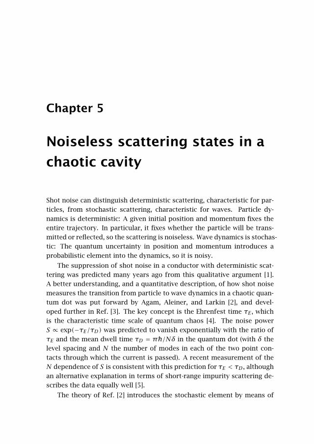
Chapter 5
Noiseless scattering states in a
chaotic cavity
Shot noise can distinguish deterministic scattering, characteristic for par-ticles, from stochastic scattering, characteristic for waves. Particle dy-namics is deterministic: A given initial position and momentum fixes theentire trajectory. In particular, it fixes whether the particle will be trans-mitted or reflected, so the scattering is noiseless. Wave dynamics is stochas-tic: The quantum uncertainty in position and momentum introduces aprobabilistic element into the dynamics, so it is noisy.
The suppression of shot noise in a conductor with deterministic scat-tering was predicted many years ago from this qualitative argument [1].A better understanding, and a quantitative description, of how shot noisemeasures the transition from particle to wave dynamics in a chaotic quan-tum dot was put forward by Agam, Aleiner, and Larkin [2], and devel-oped further in Ref. [3]. The key concept is the Ehrenfest time τE , whichis the characteristic time scale of quantum chaos [4]. The noise powerS ∝ exp(−τE/τD) was predicted to vanish exponentially with the ratio ofτE and the mean dwell time τD = π/Nδ in the quantum dot (with δ thelevel spacing and N the number of modes in each of the two point con-tacts through which the current is passed). A recent measurement of theN dependence of S is consistent with this prediction for τE < τD , althoughan alternative explanation in terms of short-range impurity scattering de-scribes the data equally well [5].
The theory of Ref. [2] introduces the stochastic element by means of
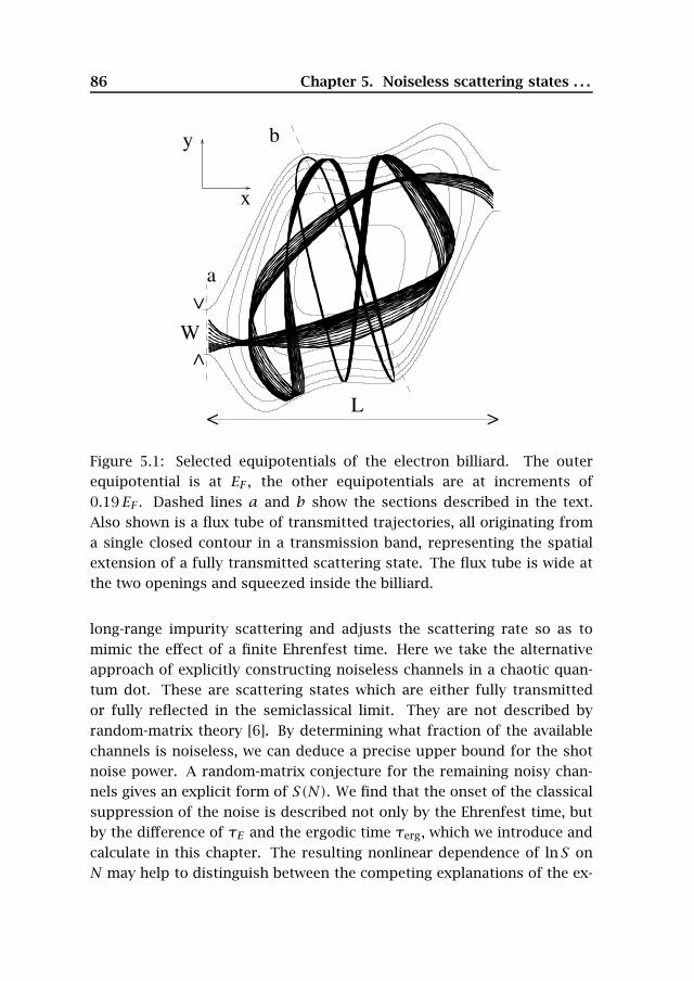
86 Chapter 5. Noiseless scattering states . . .
b
a
W
><
< >L
x
y
Figure 5.1: Selected equipotentials of the electron billiard. The outerequipotential is at EF , the other equipotentials are at increments of0.19EF . Dashed lines a and b show the sections described in the text.Also shown is a flux tube of transmitted trajectories, all originating froma single closed contour in a transmission band, representing the spatialextension of a fully transmitted scattering state. The flux tube is wide atthe two openings and squeezed inside the billiard.
long-range impurity scattering and adjusts the scattering rate so as tomimic the effect of a finite Ehrenfest time. Here we take the alternativeapproach of explicitly constructing noiseless channels in a chaotic quan-tum dot. These are scattering states which are either fully transmittedor fully reflected in the semiclassical limit. They are not described byrandom-matrix theory [6]. By determining what fraction of the availablechannels is noiseless, we can deduce a precise upper bound for the shotnoise power. A random-matrix conjecture for the remaining noisy chan-nels gives an explicit form of S(N). We find that the onset of the classicalsuppression of the noise is described not only by the Ehrenfest time, butby the difference of τE and the ergodic time τerg, which we introduce andcalculate in this chapter. The resulting nonlinear dependence of lnS onN may help to distinguish between the competing explanations of the ex-
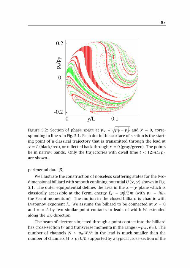
87
p y/p
F
y/L 0.10
-
-
0.2
-0.2
0
-
Figure 5.2: Section of phase space at px =√p2F − p2
y and x = 0, corre-sponding to line a in Fig. 5.1. Each dot in this surface of section is the start-ing point of a classical trajectory that is transmitted through the lead atx = L (black/red), or reflected back through x = 0 (gray/green). The pointslie in narrow bands. Only the trajectories with dwell time t < 12mL/pFare shown.
perimental data [5].
We illustrate the construction of noiseless scattering states for the two-dimensional billiard with smooth confining potentialU(x,y) shown in Fig.5.1. The outer equipotential defines the area in the x − y plane which isclassically accessible at the Fermi energy EF = p2
F/2m (with pF = kFthe Fermi momentum). The motion in the closed billiard is chaotic withLyapunov exponent λ. We assume the billiard to be connected at x = 0and x = L by two similar point contacts to leads of width W extendedalong the ±x-direction.
The beam of electrons injected through a point contact into the billiardhas cross-sectionW and transverse momenta in the range (−pW ,pW). Thenumber of channels N pWW/ in the lead is much smaller than thenumber of channelsM pFL/ supported by a typical cross-section of the
88 Chapter 5. Noiseless scattering states . . .
billiard. While W/L 1 in general, the ratio pW/pF depends on detailsof the potential near the point contact. If pW/pF 1 one speaks of acollimated beam. This is typical for a smooth potential, while a hard-wall potential typically has pW pF (no collimation). We define rmin =min (W/L,pW/pF) and rmax = max (W/L,pW/pF).
The classical phase space is four-dimensional. By restricting the energyto EF and taking x = 0 we obtain the two-dimensional section of phasespace shown in Fig. 5.2. The accessible values of y and py lie in a disc-shaped region of area Otot = Nh in this surface of section. Up to factorsof order unity, the disk has width rmin and length rmax (if coordinate andmomentum are measured in units of L and pF , respectively). In Fig. 5.2one has rmin rmax. Each point in the disc defines a classical trajectorythat enters the billiard (for positive px) and then leaves the billiard eitherthrough the same lead (reflection) or through the other lead (transmission).The points lie in narrow bands, which we will refer to as “transmissionbands” and “reflection bands”.
It is evident from Fig. 5.2 that the area Oband,j enclosed by a typicaltransmission (or reflection) band j is much less than Otot. For an estimatewe consider the time T(y, py) that elapses before transmission. Let Tj bethe dwell time averaged over the starting points y,py in a single band.The fluctuations of T around the average are of the order of the timeTW mW/pW to cross the point contact, which is typically Tj . As wewill see below, the area of the band decreases with Tj as
Oband,j O0 exp(−λTj) if Tj 1/λ, TW . (5.1)
The prefactorO0 = Ototrmin/rmax depends on the degree of collimation. Inchapter 2 the symmetric case rmin = rmax was assumed, when O0 = Otot.
We now proceed to the construction of fully transmitted scatteringstates. To this end we consider a closed contour C within a transmissionband j. The starting points on the contour define a family of trajectoriesthat form a flux tube inside the billiard (see Fig. 5.1). The semiclassicalwave function
ψ(x,y) =∑σ
√ρσ(x,y) exp[iSσ (x,y)/] (5.2)
is determined as usual from the action Sσ and density ρσ that solve theHamilton-Jacobi and continuity equations
|∇S|2 = 2m(EF −U), ∇ · (ρ∇S) = 0. (5.3)

89
0
0.5
0 10
P(T
)
T
< >τerg
<>TW
lnP
t0 50
-5
-3 slope 1/τD
<
Figure 5.3: Dwell time distribution for the billiard of Fig. 5.1. Electronsat the Fermi energy are injected through the left lead. Time is in units ofmL/pF . Inset: the same data on a semilogarithmic scale with larger binsize of the histogram. Three characteristic time scales are seen: TW , τerg,τD.
The action is multivalued and the index σ labels the different sheets. Typ-ically, there are two sheets, one originating from the upper half of thecontour C and one from the lower half.
The requirement that ψ is single-valued as one winds around the con-tour imposes a quantization condition on the enclosed area,
∮Cpydy = (n+ 1/2)h. (5.4)
The increment 1/2 accounts for the phase shift acquired at the two turn-ing points on the contour. The quantum number n = 0,1,2, . . . is thechannel index. The largest value of n occurs for a contour enclosing anarea Oband,j . The number of transmission channels Nj within band j istherefore given by Oband,j/h, with an accuracy of order unity. In view ofEq. (5.1) we have
Nj (O0/h) exp(−λTj), for Tj < τE, (5.5a)
Nj = 0, for Tj > τE. (5.5b)
90 Chapter 5. Noiseless scattering states . . .
The time
τE = λ−1 [ln(2O0/h)+O(1)] = λ−1 [ln(Nrmin/rmax)+O(1)] (5.6)
above which there are no fully transmitted channels is the Ehrenfest timeof this problem.
By decomposing one of these Nj scattering states into a given basis oftransverse modes in the lead one constructs an eigenvector of the trans-mission matrix product tt†. The corresponding eigenvalue Tj,n equalsunity with exponential accuracy in the semiclassical limit n 1. Becauseof the degeneracy of this eigenvalue any linear combination of eigenvec-tors is again an eigenvector. This manifests itself in our construction asan arbitrariness in the choice of C.
We observe in Fig. 5.1 that the spatial density profile ρ(x,y) of a fullytransmitted scattering state is highly non-uniform. The flux tube is broad(width of order W ) at the two openings, but is squeezed down to verysmall width inside the billiard. A similar effect was noted in chapter 2 forthe excited states of an Andreev billiard. Following the same argument weestimate the minimal width of the flux tube as Wmin L
√Nj/kFL.
The total number
Ncl =∑jNj = N
∫ τE0P(T)dT (5.7)
of fully transmitted and reflected channels is determined by the dwell timedistribution P(T) [7]. Fig. 5.3 shows this distribution in our billiard. Onesees three different time scales. The narrow peaks represent individualtransmission (reflection) bands. They consist of an abrupt jump followedby an exponential decay with time constant TW . These exponential tailscorrespond to the borders of the bands, where the trajectory bouncesmany times between the sides of the point contact. If we smooth P(T)over such short time intervals, an exponential decay with time constantτD = π/Nδ is obtained (inset). The decay starts at the so called “ergodictime” τerg. There are no trajectories leaving the cavity for T < τerg. So thesmoothed dwell time distribution has the form.
P(T) = τ−1D exp[(τerg − T)/τD]θ(T − τerg), (5.8)
with θ(x) the unit step function.
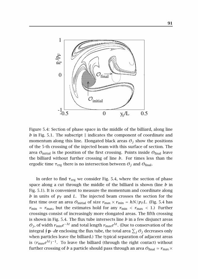
91
-1
0
1
-0.5 0 0.5y /L
p /p
F
Oinitial
Ofinal>
>
Figure 5.4: Section of phase space in the middle of the billiard, along lineb in Fig. 5.1. The subscript ‖ indicates the component of coordinate andmomentum along this line. Elongated black areas Oj show the positionsof the 5-th crossing of the injected beam with this surface of section. Thearea Oinitial is the position of the first crossing. Points inside Ofinal leavethe billiard without further crossing of line b. For times less than theergodic time τerg there is no intersection between Oj and Ofinal.
In order to find τerg we consider Fig. 5.4, where the section of phasespace along a cut through the middle of the billiard is shown (line b inFig. 5.1). It is convenient to measure the momentum and coordinate alongb in units of pF and L. The injected beam crosses the section for thefirst time over an area Oinitial of size rmax × rmin = hN/pFL. (Fig. 5.4 hasrmin rmax, but the estimates hold for any rmin < rmax < 1.) Furthercrossings consist of increasingly more elongated areas. The fifth crossingis shown in Fig. 5.4. The flux tube intersects line b in a few disjunct areasOj , of width rmine−λt and total length rmaxeλt . (Due to conservation of theintegral
∮p·dr enclosing the flux tube, the total area
∑j Oj decreases only
when particles leave the billiard.) The typical separation of adjacent areasis (rmaxeλt)−1. To leave the billiard (through the right contact) withoutfurther crossing of b a particle should pass through an area Ofinal rmax×
92 Chapter 5. Noiseless scattering states . . .
rmin. This is highly improbable [8] until the separation of the areas Ojbecomes of order rmax, leading to the ergodic time
τerg = λ−1 ln r−2max. (5.9)
The ergodic time varies from τerg λ−1 for rmax 1 to τerg = λ−1 ln(kFL/N)for rmin rmax. The overlap of the areas Oj and Ofinal is the mappingof the transmission band onto the surface of section b. It has an areapFLr 2
mine−λt = Otot(rmin/rmax)e−λt , leading to Eq. (5.1).
Substituting Eq. (5.8) into Eq. (5.7) we arrive at the number Ncl of fullytransmitted and reflected channels,
Ncl = Nθ(τE − τerg)[1− e(τerg−τE)/τD
], (5.10)
τE − τerg λ−1 ln(N2/kFL). (5.11)
There are no fully transmitted or reflected channels if τE < τerg, hence ifN <
√kFL. Notice that the dependence of τE and τerg separately on the
degree of collimation drops out of the difference τE − τerg. The numberof noiseless channels is therefore insensitive to details of the confiningpotential. An Ehrenfest time ∝ ln(N2/kFL) has appeared before in con-nection with the Andreev billiard [9], but the role of collimation (and theassociated finite ergodic time) was not considered there.
Eqs. (5.5) and (5.8) imply that the majority of noiseless channels groupin bands having Nj 1, which justifies the semiclassical approximation.The total number of these noiseless bands is of the order of (N−Ncl)/λτD ,which is much less than both N −Ncl and Ncl. Because of this inequalitythe relatively short trajectories contributing to the noiseless channels arewell separated in phase space from other, longer trajectories (cf. Fig. 5.2).
The shot-noise power S is related to the transmission eigenvalues by[10]
S = 2eIg−1N∑k=1
Tk(1−Tk), (5.12)
with I the time-averaged current and g = ∑kTk the dimensionless con-ductance. The Ncl fully transmitted or reflected channels have Tk = 1 or0, hence they do not contribute to the noise. The remaining N −Ncl chan-nels contribute at most 1/4 per channel to Sg/2eI . Using that g = N/2 forlargeN, we arrive at an upper bound for the noise power S < eI(1−Ncl/N).
93
For a more quantitative description of the noise power we need toknow the distribution P(T ) of the transmission eigenvalues for the N−Nclnoisy channels, which can not be described semiclassically. We expect thedistribution to have the same bimodal form P(T ) = π−1T −1/2(1−T )−1/2
as in the case Ncl = 0 [6]. This expectation is motivated by the earlier ob-servation that the Ncl noiseless channels are well separated in phase spacefrom the N−Ncl noisy ones. Using this form of P(T ) we find that the con-tribution to Sg/2eI per noisy channel equals
∫ 10 T (1−T )P(T )dT = 1/8,
half the maximum value. The Fano factor F = S/2eI is thus estimated as
F = 14 , for N
√kFL, (5.13a)
F = 14(kFL/N
2)Nδ/πλ, for N √kFL. (5.13b)
This result should be compared with that of Ref. [2]: F ′ = 14(kFL)
−Nδ/πλ.The ratio F ′/F = exp[(2Nδ/πλ) ln(N/kFL)] is always close to unity (be-cause Nδ/πλ N/kFL 1). But F − 1
4 and F ′ − 14 are entirely different
for N √kFL, which is the relevant regime in the experiment [5]. There
the N dependence of the shot noise was fitted as F = 14(1 − tQ/τD) =
14(1 − constant × N), where tQ is some N-independent time. Eq. (5.13)predicts a more complex N dependence, a plateau followed by a decreaseas lnF ∝ −N ln(N2/kFL), which could be observable if the experimentextends over a larger range of N.
We mention two other experimentally observable features of the theorypresented here. The reduction of the Fano factor described by Eq. (5.13)is the cumulative effect of many noiseless bands. The appearance of newbands with increasing N introduces a fine structure in F(N), consisting ofa series of cusps with a square-root singularity near the cusp. The sec-ond feature is the highly nonuniform spatial extension of open channels,evident in Fig. 5.1, which could be observed with the STM technique ofRef. [11]. From a more general perspective the noiseless channels con-structed in this chapter show that the random-matrix approach may beused in ballistic systems only for sufficiently small openings: N
√kFL is
required. For larger N the scattering becomes deterministic, rather thanstochastic, and random-matrix theory starts to break down.
94 Chapter 5. Noiseless scattering states . . .
Bibliography
[1] C. W. J. Beenakker and H. van Houten, Phys. Rev. B 43, 12066 (1991).
[2] O. Agam, I. Aleiner, and A. Larkin, Phys. Rev. Lett. 85, 3153 (2000).
[3] H.-S. Sim, and H. Schomerus, Phys. Rev. Lett. 89, 066801 (2002); R. G.Nazmitdinov, H.-S. Sim, H. Schomerus, and I. Rotter, Phys. Rev. B 66,241302(R) (2002).
[4] G. M. Zaslavsky, Phys. Rep. 80, 157 (1981).
[5] S. Oberholzer, E. V. Sukhorukov, and C. Schonenberger, Nature 415,765 (2002).
[6] R. A. Jalabert, J.-L. Pichard, and C. W. J. Beenakker, Europhys. Lett. 27,255 (1994).
[7] The dwell time distribution is defined with a uniform measure in thesurface of section of the lead, so that its integral is directly propor-tional to the number of channels. The mean dwell time τD = π/Nδwas calculated by W. Bauer and G. F. Bertsch, Phys. Rev. Lett. 65, 2213(1990).
[8] Dwell times shorter than τerg are improbable but they may exist forspecial positions of the two point contacts. The probability that arandom position permits a transmitted (or reflected) trajectory of du-ration T < τerg is exp[−λ(τerg − T)].
[9] M. G. Vavilov and A. I. Larkin, Phys. Rev. B 67, 115335 (2003).
[10] M. Buttiker, Phys. Rev. Lett. 65, 2901 (1990).
[11] M. A. Topinka et. al., Nature 410, 183 (2001).

96 Bibliography
Chapter 6
Spectroscopy of a driven
solid-state qubit coupled to a
structured environment
6.1 Introduction
Currently, we witness an impressive progress in realizing coherent quan-tum dynamics of macroscopic solid state devices [1–5]. Very recently, ex-perimental results on the quantum dynamics of a superconducting fluxqubit coupled to a read-out Superconducting Quantum Interference De-vice (SQUID) have been reported [6]. The flux qubit consists of a supercon-ducting ring with three Josephson junctions and, in the proper parame-ter regime, it forms a quantum mechanical macroscopic two-state system(TSS). An external time-dependent driving force controls the state of theTSS. A SQUID couples inductively to the qubit and, together with an ex-ternal shunt capacitance, it can be modeled as a harmonic oscillator (HO).Due to the coupling of the SQUID to the surrounding environment, theharmonic oscillator is (weakly) damped. The state of the qubit can be in-ferred from the state of the SQUID. The experiment provides spectroscopicdata on the different transition frequencies of the coupled TSS-HO device.Moreover, Rabi oscillations involving different pairs of quantum states ofthe device have been revealed, including the so-termed red and blue side-band transitions between energy states of the coupled TSS-HO system.
Heading for a comprehensive detailed understanding, a quantitative
98 Chapter 6. Spectroscopy of a driven solid-state . . .
modeling which includes the effects of time-dependent driving, decoher-ence and dissipation is required. In this chapter we give a descriptionwhich goes beyond the well-known Jaynes-Cummings model [7], by avoid-ing the strong rotating-wave approximation and by including a micro-scopic model for the environment. A generic theoretical model for study-ing the environmental effects on a driven TSS is the driven spin-bosonmodel [8,9]. The environment is characterized by a spectral density J(ω).The widest used form is that of an Ohmic spectral density, where J(ω)is proportional to the frequency ω. It mimics the effects of an unstruc-tured Ohmic electromagnetic environment. In the classical limit this leadsto white noise and all transitions in the system are damped equally. How-ever, if the environment for the qubit is formed by a quantum measuringdevice which itself is damped by Ohmic fluctuations, the simple descrip-tion as an Ohmic environment might become inappropriate. In particular,the SQUID-detector being well described as a HO can equally well be con-sidered as a (broadened) localized mode of the environment influencingthe qubit as the central quantum system. In this picture, the plasma res-onance at frequency Ωp of the SQUID gives rise to a non-Ohmic effectivespectral density Jeff(ω) for the qubit with a Lorentzian peak at the plasmafrequency of the detector [10].
The effects of such a structured spectral density on decoherence havebeen investigated in several theoretical works in various limits. The roleof the external driving being in resonance with the symmetric TSS at zerotemperature has been studied in Ref. [11] within a Bloch-Redfield formal-ism being equivalent to a perturbative approach in Jeff. Smirnov’s analy-sis [12] is based on the assumption of weak interaction between the TSSand the HO being equivalent to a perturbative approach in Jeff as well.Moreover, a rotating-wave approximation is used. The first assumption,however, might become problematic if the driven TSS is in resonance withthe HO. The results presented in Refs. [13, 14] reveal in fact, for the un-driven case, that a perturbative approach in Jeff breaks down for strongqubit-detector coupling, and when the qubit and detector frequencies arecomparable. Dephasing times at zero temperature have been determinedfor the undriven spin-boson model with a structured environment in Ref.[15] within a numerical flow equation method.
As shown in the experiment of Ref. [6], the interplay between the ex-ternal driving and the dynamics of the coupled TSS-HO system yields to
6.1 Introduction 99
additional multi-photon transitions, which can be explained only by con-sidering the spectrum of the coupled system. In contrast, if the time-scaleof the HO does not play a role, the multi-photon resonances occur in thedriven qubit solely, which happens when the driving frequency (or integermultiples of it) matches the characteristic energy scales of the qubit [9].Such multiphoton resonances can be experimentally detected in an ac-driven flux qubit by measuring the asymptotic occupation probabilities ofthe qubit, as the dc-field is varied [16]. These qubit resonances, which havealso been theoretically investigated within a Bloch equation formalism inRef. [17], could be explained in terms of intrinsic transitions in a drivenspin-boson system with an unstructured environment.
In this chapter, we provide a comprehensive theoretical description ofthe driven spin-boson system in the presence of a structured environmentwith one localized mode. Upon making use of the equivalence of thisgeneric model with the model of a driven TSS coupled to an Ohmicallydamped HO, we first consider the experimentally most interesting caseof low temperature and weak damping of the HO while the coupling be-tween the TSS and the HO is kept arbitrary. In this regime, a Floquet-Born-Markov master equation can be established for the driven TSS-HO system.A restriction to the most relevant energy states allows the analytic calcu-lation of the asymptotic TSS time-averaged population P∞, including theexplicit shape of the resonance peaks and dips. We furthermore considerthe case of strong damping and/or high temperature which is the comple-mentary parameter regime. An analytic real-time path-integral approachwithin the non-interacting blip approximation for the driven TSS with theLorentzian-shaped spectral density allows to analytically determine P∞ aswell. We compare the results obtained from closed analytic expressionswith those of numerically exact real-time QUAPI calculations in both pa-rameter regimes and find a very good agreement validating our analyticalapproaches. Finally, we consider the weakly damped TSS with the localizedmode in the limit of large HO frequencies. Then, the localized mode acts asa high-frequency cutoff and the usual Ohmically damped driven TSS is re-covered. For this case, we employ an approximation valid for large drivingfrequencies and obtain a simple expression for the resonance line shapesfor multi-photon transitions. Most importantly, we find that the width ofthe n-photon resonance scales with the n-th ordinary Bessel function.
The chapter is organized as follows: In Sec. 6.2, we present the theo-
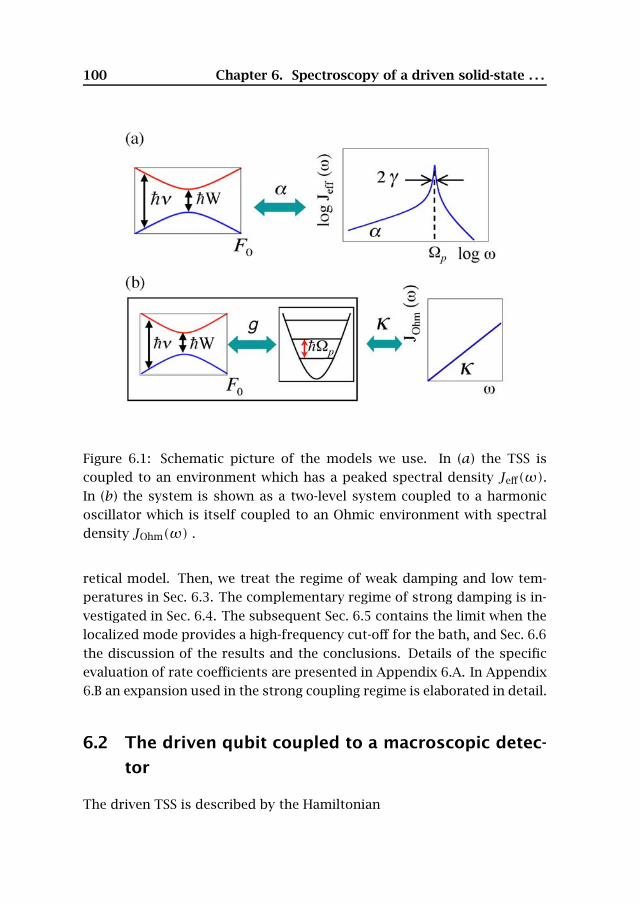
100 Chapter 6. Spectroscopy of a driven solid-state . . .
Figure 6.1: Schematic picture of the models we use. In (a) the TSS iscoupled to an environment which has a peaked spectral density Jeff(ω).In (b) the system is shown as a two-level system coupled to a harmonicoscillator which is itself coupled to an Ohmic environment with spectraldensity JOhm(ω) .
retical model. Then, we treat the regime of weak damping and low tem-peratures in Sec. 6.3. The complementary regime of strong damping is in-vestigated in Sec. 6.4. The subsequent Sec. 6.5 contains the limit when thelocalized mode provides a high-frequency cut-off for the bath, and Sec. 6.6the discussion of the results and the conclusions. Details of the specificevaluation of rate coefficients are presented in Appendix 6.A. In Appendix6.B an expansion used in the strong coupling regime is elaborated in detail.
6.2 The driven qubit coupled to a macroscopic detec-
tor
The driven TSS is described by the Hamiltonian
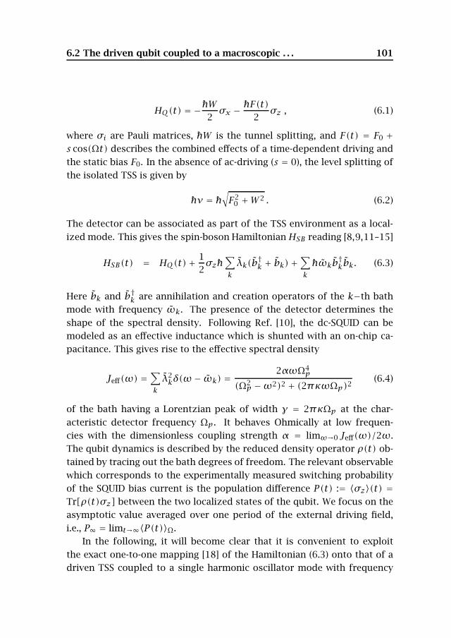
6.2 The driven qubit coupled to a macroscopic . . . 101
HQ(t) = −W2 σx − F(t)2σz , (6.1)
where σi are Pauli matrices, W is the tunnel splitting, and F(t) = F0 +s cos(Ωt) describes the combined effects of a time-dependent driving andthe static bias F0. In the absence of ac-driving (s = 0), the level splitting ofthe isolated TSS is given by
ν = √F2
0 +W 2 . (6.2)
The detector can be associated as part of the TSS environment as a local-ized mode. This gives the spin-boson HamiltonianHSB reading [8,9,11–15]
HSB(t) = HQ(t)+ 12σz
∑kλk(b
†k + bk)+
∑kωkb
†kbk. (6.3)
Here bk and b†k are annihilation and creation operators of the k−th bathmode with frequency ωk. The presence of the detector determines theshape of the spectral density. Following Ref. [10], the dc-SQUID can bemodeled as an effective inductance which is shunted with an on-chip ca-pacitance. This gives rise to the effective spectral density
Jeff(ω) =∑kλ2kδ(ω− ωk) =
2αωΩ4p
(Ω2p −ω2)2 + (2πκωΩp)2
(6.4)
of the bath having a Lorentzian peak of width γ = 2πκΩp at the char-acteristic detector frequency Ωp. It behaves Ohmically at low frequen-cies with the dimensionless coupling strength α = limω→0 Jeff(ω)/2ω.The qubit dynamics is described by the reduced density operator ρ(t) ob-tained by tracing out the bath degrees of freedom. The relevant observablewhich corresponds to the experimentally measured switching probabilityof the SQUID bias current is the population difference P(t) := 〈σz〉(t) =Tr[ρ(t)σz] between the two localized states of the qubit. We focus on theasymptotic value averaged over one period of the external driving field,i.e., P∞ = limt→∞〈P(t)〉Ω.
In the following, it will become clear that it is convenient to exploitthe exact one-to-one mapping [18] of the Hamiltonian (6.3) onto that of adriven TSS coupled to a single harmonic oscillator mode with frequency
102 Chapter 6. Spectroscopy of a driven solid-state . . .
Ωp with interaction strength g. The HO itself interacts with a set of mutu-ally non-interacting harmonic oscillators. The corresponding total Hamil-tonian is then
HQOB(t) = HQO(t)+HOB (6.5)
with
HQO(t) = HQ(t)+ gσz(B† + B)+ ΩpB†B ,
HOB = (B† + B)∑kνk(b
†k + bk)+
∑kωkb
†kbk + (B† + B)2
∑kν2kωk
,
(6.6)
where we have omitted the zero-point constant energy terms. Here, B andB† are the annihilation and creation operators of the localized HO mode,while bk and b†k are the corresponding bath mode operators. The spectraldensity of the continuous bath modes is now Ohmic with dimensionlessdamping strength κ, i.e.,
JOhm(ω) =∑kν2kδ(ω−ωk) = κω
ω2D
ω2 +ω2D, (6.7)
where we have introduced a high-frequency Drude cut-off at frequencyωD. If ωD is larger than all other energy scales the particular choice ofcut-off does not influence the results at long times. The relation betweeng and α follows as g = Ωp
√α/(8κ). Fig. 6.1 illustrates a sketch of the
two equivalent descriptions of the system. Fig. 6.1a shows the viewpointwhere the localized mode is part of the environmental modes, while Fig.6.1b depicts the perspective of the localized mode being part of the “cen-tral” quantum system which itself is coupled to an Ohmic environment.The equivalence of both standpoints has first been pointed out by Garg etal. [18] in the context of electron transfer in chemical physics. As shownbelow, the first way is more convenient for the description in terms of ana-lytic real-time path-integrals (Sec. 6.4), while the second viewpoint is moreappropriate for the regime of weak-coupling and for the numerical treat-ment with QUAPI (see below). Note that the TSS reduced density operatorρ(t) is obtained after tracing out the degrees of freedom of the bath andof the HO. Further progress relies on approximations which depend on thechoice of the various parameters.
6.3 Weak coupling: Floquet-Born-Markov master equation 103
6.3 Weak coupling: Floquet-Born-Markov master equa-
tion
If the coupling between the HO and the bath is weak, i.e., κ 1 , wecan choose an approach in terms of a Born-Markov master equation in anextended Floquet description [9, 19, 20]. For a self-contained discussion,we shortly introduce below the required formalism of the Floquet theory.The interested reader can find more details in the review in Ref. [9].
6.3.1 Floquet formalism and Floquet-Born-Markovian master equa-tion
For systems with periodic driving it is convenient to use the Floquet for-malism that allows to treat periodic forces of arbitrary strength and fre-quency [19]. It is based on the fact that the eigenstates of a periodic Hamil-tonian HQO(t) = HQO(t + 2π/Ω) are of the form
|ψ(t)〉 = e−iεαt/|φα(t)〉 ,|φα(t)〉 = |φα(t + 2π/Ω)〉 , (6.8)
with the Floquet states |φα(t)〉 being periodic in time (as is the Hamilto-nian) and εα are called the Floquet or quasi-energies. They can be obtainedfrom the eigenvalue equation
(HQO(t)− i ∂∂t
)|φα(t)〉 = εα|φα(t)〉. (6.9)
If the quasi-energy εα is an eigenvalue with Floquet state |φα(t)〉, so isεα + nΩ with Floquet state exp (inΩt)|φα(t)〉. Both Floquet states cor-respond to the same physical state. Because of their periodicity both theFloquet states and the Hamiltonian can be written as a Fourier series, i.e.,
|φα(t)〉 =∑n|φ(n)α 〉 exp (inΩt) ,
HQO(t) =∑nH(n)QO exp (inΩt). (6.10)
Substituting these Fourier decompositions in the eigenvalue equation (6.9)gives [21]
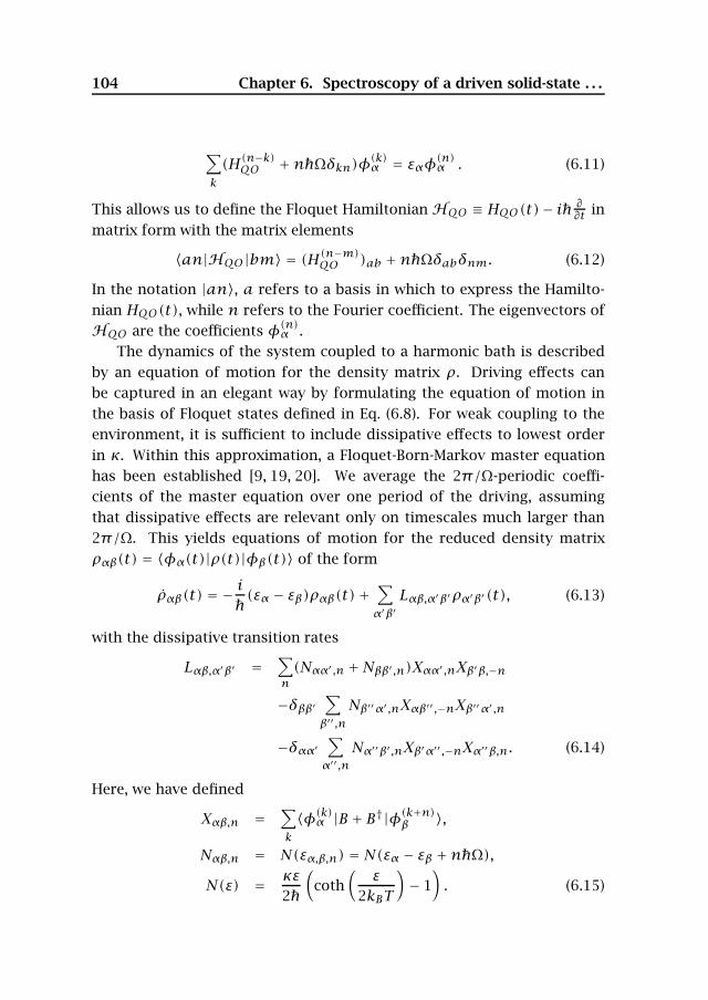
104 Chapter 6. Spectroscopy of a driven solid-state . . .
∑k(H(n−k)QO +nΩδkn)φ(k)α = εαφ(n)α . (6.11)
This allows us to define the Floquet Hamiltonian HQO ≡ HQO(t)− i ∂∂t inmatrix form with the matrix elements
〈an|HQO|bm〉 = (H(n−m)QO )ab +nΩδabδnm. (6.12)
In the notation |an〉, a refers to a basis in which to express the Hamilto-nian HQO(t), while n refers to the Fourier coefficient. The eigenvectors ofHQO are the coefficients φ(n)α .
The dynamics of the system coupled to a harmonic bath is describedby an equation of motion for the density matrix ρ. Driving effects canbe captured in an elegant way by formulating the equation of motion inthe basis of Floquet states defined in Eq. (6.8). For weak coupling to theenvironment, it is sufficient to include dissipative effects to lowest orderin κ. Within this approximation, a Floquet-Born-Markov master equationhas been established [9, 19, 20]. We average the 2π/Ω-periodic coeffi-cients of the master equation over one period of the driving, assumingthat dissipative effects are relevant only on timescales much larger than2π/Ω. This yields equations of motion for the reduced density matrixραβ(t) = 〈φα(t)|ρ(t)|φβ(t)〉 of the form
ραβ(t) = −i(εα − εβ)ραβ(t)+
∑α′β′
Lαβ,α′β′ρα′β′(t), (6.13)
with the dissipative transition rates
Lαβ,α′β′ =∑n(Nαα′ ,n +Nββ′,n)Xαα′ ,nXβ′β,−n
−δββ′∑β′′,n
Nβ′′α′,nXαβ′′ ,−nXβ′′α′,n
−δαα′∑α′′,n
Nα′′β′,nXβ′α′′ ,−nXα′′β,n. (6.14)
Here, we have defined
Xαβ,n =∑k〈φ(k)α |B + B†|φ(k+n)β 〉,
Nαβ,n = N(εα,β,n) = N(εα − εβ +nΩ),N(ε) = κε
2
(coth
(ε
2kBT
)− 1). (6.15)
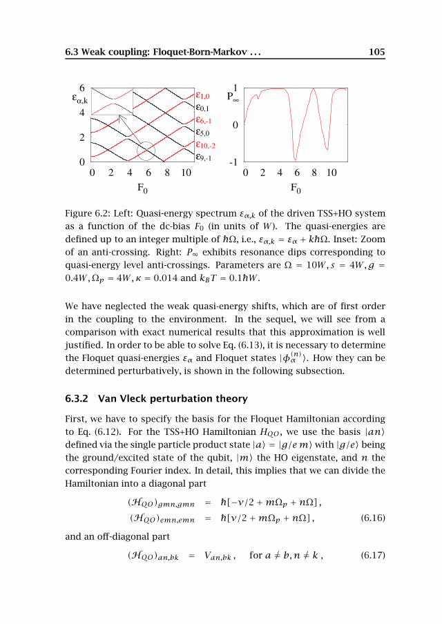
6.3 Weak coupling: Floquet-Born-Markov . . . 105
0
2
4
6
0 2 4 6 8 10
F0
εα,kε1,0
ε0,1
ε6,-1
ε5,0
ε10,-2
ε9,-1 -1
0
1
0 2 4 6 8 10
F0
P∞
Figure 6.2: Left: Quasi-energy spectrum εα,k of the driven TSS+HO systemas a function of the dc-bias F0 (in units of W ). The quasi-energies aredefined up to an integer multiple of Ω, i.e., εα,k = εα + kΩ. Inset: Zoomof an anti-crossing. Right: P∞ exhibits resonance dips corresponding toquasi-energy level anti-crossings. Parameters are Ω = 10W, s = 4W,g =0.4W,Ωp = 4W,κ = 0.014 and kBT = 0.1W .
We have neglected the weak quasi-energy shifts, which are of first orderin the coupling to the environment. In the sequel, we will see from acomparison with exact numerical results that this approximation is welljustified. In order to be able to solve Eq. (6.13), it is necessary to determinethe Floquet quasi-energies εα and Floquet states |φ(n)α 〉. How they can bedetermined perturbatively, is shown in the following subsection.
6.3.2 Van Vleck perturbation theory
First, we have to specify the basis for the Floquet Hamiltonian accordingto Eq. (6.12). For the TSS+HO Hamiltonian HQO , we use the basis |an〉defined via the single particle product state |a〉 = |g/em〉with |g/e〉 beingthe ground/excited state of the qubit, |m〉 the HO eigenstate, and n thecorresponding Fourier index. In detail, this implies that we can divide theHamiltonian into a diagonal part
(HQO)gmn,gmn = [−ν/2+mΩp +nΩ] ,(HQO)emn,emn = [ν/2+mΩp +nΩ] , (6.16)
and an off-diagonal part
(HQO)an,bk = Van,bk , for a = b,n = k , (6.17)
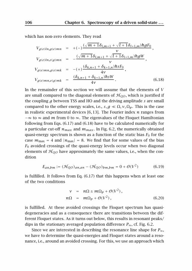
106 Chapter 6. Spectroscopy of a driven solid-state . . .
which has non-zero elements. They read
Vg(e)ln,g(e)mn = +(−)(√m+ 1δl,m+1 +
√l+ 1δl+1,m)gF0
ν,
Vg(e)ln,e(g)mn = −(√m+ 1δl,m+1 +
√l+ 1δl+1,m)gW
ν,
Vg(e)mn,g(e)mk = −(+)(δk,n+1 + δk+1,n)sF0
4ν,
Vg(e)mn,e(g)mk = (δk,n+1 + δk+1,n)sW4ν
. (6.18)
In the remainder of this section we will assume that the elements of Vare small compared to the diagonal elements of HQO , which is justified ifthe coupling g between TSS and HO and the driving amplitude s are smallcompared to the other energy scales, i.e., s, g Ω, ν,Ωp. This is the casein realistic experimental devices [6, 13]. The Fourier index n ranges from−∞ to ∞ and m from 0 to ∞. The eigenvalues of the Floquet Hamiltonianfollowing from Eqs. (6.17) and (6.18) have to be calculated numerically fora particular cut-off nmax and mmax . In Fig. 6.2, the numerically obtainedquasi-energy spectrum is shown as a function of the static bias F0 for thecase mmax = 4 and |nmax| = 8. We find that for some values of the biasF0 avoided crossings of the quasi-energy levels occur when two diagonalelements of HQO have approximately the same values, i.e., when the con-dition
Ean,bm := (HQO)an,an − (HQO)bm,bm = 0+O(V 2) (6.19)
is fulfilled. It follows from Eq. (6.17) that this happens when at least oneof the two conditions
ν = nΩ±mΩp +O(V 2) ,
nΩ = mΩp +O(V 2) , (6.20)
is fulfilled. At these avoided crossings the Floquet spectrum has quasi-degeneracies and as a consequence there are transitions between the dif-ferent Floquet states. As it turns out below, this results in resonant peaks/dips in the stationary averaged population difference P∞, cf. Fig. 6.2.
Since we are interested in describing the resonance line shape for P∞,we have to determine the quasi-energies and Floquet states around a reso-nance, i.e., around an avoided crossing. For this, we use an approach which
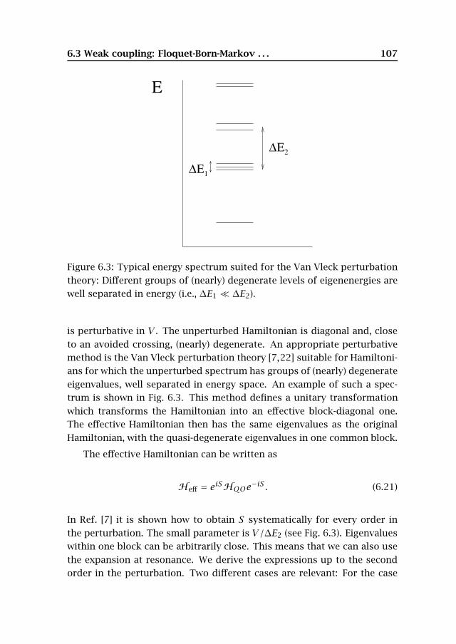
6.3 Weak coupling: Floquet-Born-Markov . . . 107
E
∆Ε
∆Ε2
1
Figure 6.3: Typical energy spectrum suited for the Van Vleck perturbationtheory: Different groups of (nearly) degenerate levels of eigenenergies arewell separated in energy (i.e., ∆E1 ∆E2).
is perturbative in V . The unperturbed Hamiltonian is diagonal and, closeto an avoided crossing, (nearly) degenerate. An appropriate perturbativemethod is the Van Vleck perturbation theory [7,22] suitable for Hamiltoni-ans for which the unperturbed spectrum has groups of (nearly) degenerateeigenvalues, well separated in energy space. An example of such a spec-trum is shown in Fig. 6.3. This method defines a unitary transformationwhich transforms the Hamiltonian into an effective block-diagonal one.The effective Hamiltonian then has the same eigenvalues as the originalHamiltonian, with the quasi-degenerate eigenvalues in one common block.
The effective Hamiltonian can be written as
Heff = eiSHQOe−iS . (6.21)
In Ref. [7] it is shown how to obtain S systematically for every order inthe perturbation. The small parameter is V/∆E2 (see Fig. 6.3). Eigenvalueswithin one block can be arbitrarily close. This means that we can also usethe expansion at resonance. We derive the expressions up to the secondorder in the perturbation. Two different cases are relevant: For the case
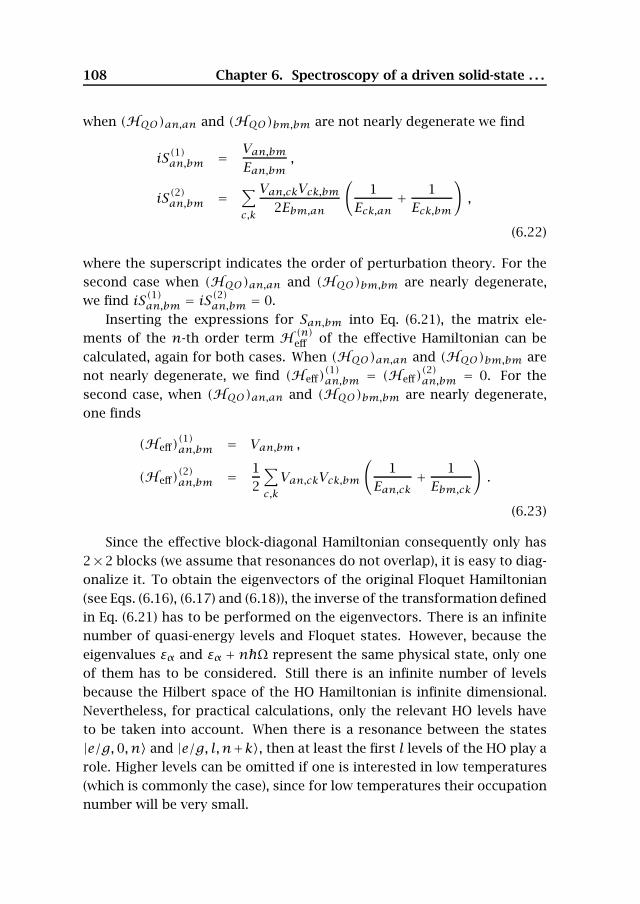
108 Chapter 6. Spectroscopy of a driven solid-state . . .
when (HQO)an,an and (HQO)bm,bm are not nearly degenerate we find
iS(1)an,bm = Van,bmEan,bm
,
iS(2)an,bm =∑c,k
Van,ckVck,bm2Ebm,an
(1
Eck,an+ 1Eck,bm
),
(6.22)
where the superscript indicates the order of perturbation theory. For thesecond case when (HQO)an,an and (HQO)bm,bm are nearly degenerate,we find iS(1)an,bm = iS
(2)an,bm = 0.
Inserting the expressions for San,bm into Eq. (6.21), the matrix ele-ments of the n-th order term H (n)
eff of the effective Hamiltonian can becalculated, again for both cases. When (HQO)an,an and (HQO)bm,bm arenot nearly degenerate, we find (Heff)
(1)an,bm = (Heff)
(2)an,bm = 0. For the
second case, when (HQO)an,an and (HQO)bm,bm are nearly degenerate,one finds
(Heff)(1)an,bm = Van,bm ,
(Heff)(2)an,bm = 1
2
∑c,kVan,ckVck,bm
(1
Ean,ck+ 1Ebm,ck
).
(6.23)
Since the effective block-diagonal Hamiltonian consequently only has2×2 blocks (we assume that resonances do not overlap), it is easy to diag-onalize it. To obtain the eigenvectors of the original Floquet Hamiltonian(see Eqs. (6.16), (6.17) and (6.18)), the inverse of the transformation definedin Eq. (6.21) has to be performed on the eigenvectors. There is an infinitenumber of quasi-energy levels and Floquet states. However, because theeigenvalues εα and εα + nΩ represent the same physical state, only oneof them has to be considered. Still there is an infinite number of levelsbecause the Hilbert space of the HO Hamiltonian is infinite dimensional.Nevertheless, for practical calculations, only the relevant HO levels haveto be taken into account. When there is a resonance between the states|e/g, 0, n〉 and |e/g, l,n+k〉, then at least the first l levels of the HO play arole. Higher levels can be omitted if one is interested in low temperatures(which is commonly the case), since for low temperatures their occupationnumber will be very small.
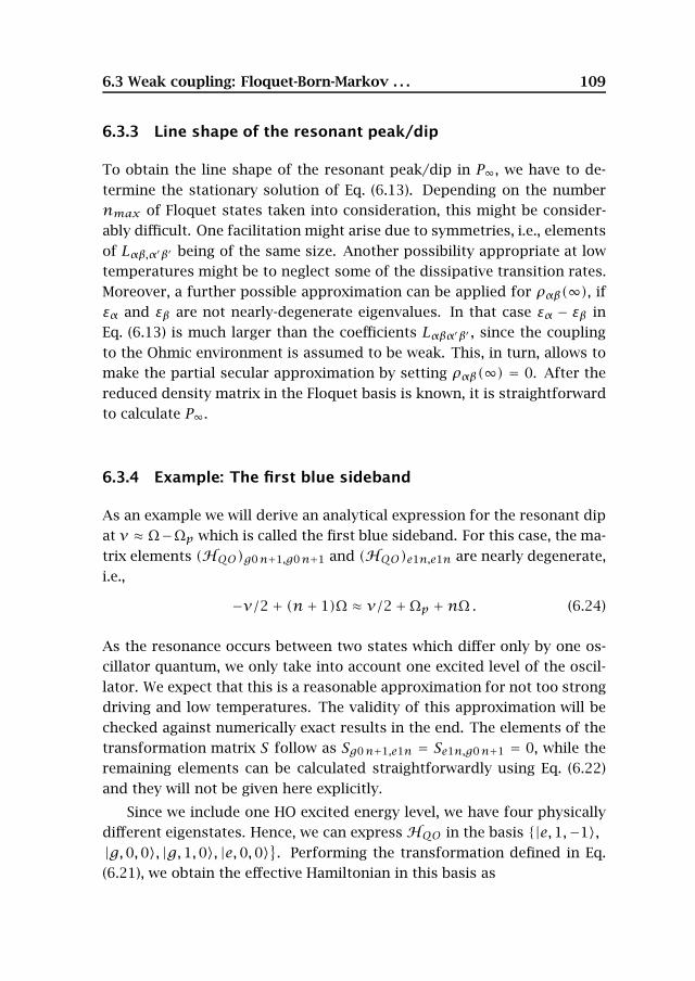
6.3 Weak coupling: Floquet-Born-Markov . . . 109
6.3.3 Line shape of the resonant peak/dip
To obtain the line shape of the resonant peak/dip in P∞, we have to de-termine the stationary solution of Eq. (6.13). Depending on the numbernmax of Floquet states taken into consideration, this might be consider-ably difficult. One facilitation might arise due to symmetries, i.e., elementsof Lαβ,α′β′ being of the same size. Another possibility appropriate at lowtemperatures might be to neglect some of the dissipative transition rates.Moreover, a further possible approximation can be applied for ραβ(∞), ifεα and εβ are not nearly-degenerate eigenvalues. In that case εα − εβ inEq. (6.13) is much larger than the coefficients Lαβα′β′ , since the couplingto the Ohmic environment is assumed to be weak. This, in turn, allows tomake the partial secular approximation by setting ραβ(∞) = 0. After thereduced density matrix in the Floquet basis is known, it is straightforwardto calculate P∞.
6.3.4 Example: The first blue sideband
As an example we will derive an analytical expression for the resonant dipat ν ≈ Ω−Ωp which is called the first blue sideband. For this case, the ma-trix elements (HQO)g0n+1,g0n+1 and (HQO)e1n,e1n are nearly degenerate,i.e.,
−ν/2 + (n+ 1)Ω ≈ ν/2+Ωp +nΩ . (6.24)
As the resonance occurs between two states which differ only by one os-cillator quantum, we only take into account one excited level of the oscil-lator. We expect that this is a reasonable approximation for not too strongdriving and low temperatures. The validity of this approximation will bechecked against numerically exact results in the end. The elements of thetransformation matrix S follow as Sg0n+1,e1n = Se1n,g0n+1 = 0, while theremaining elements can be calculated straightforwardly using Eq. (6.22)and they will not be given here explicitly.
Since we include one HO excited energy level, we have four physicallydifferent eigenstates. Hence, we can express HQO in the basis |e,1,−1〉,|g,0,0〉, |g,1,0〉, |e,0,0〉. Performing the transformation defined in Eq.(6.21), we obtain the effective Hamiltonian in this basis as
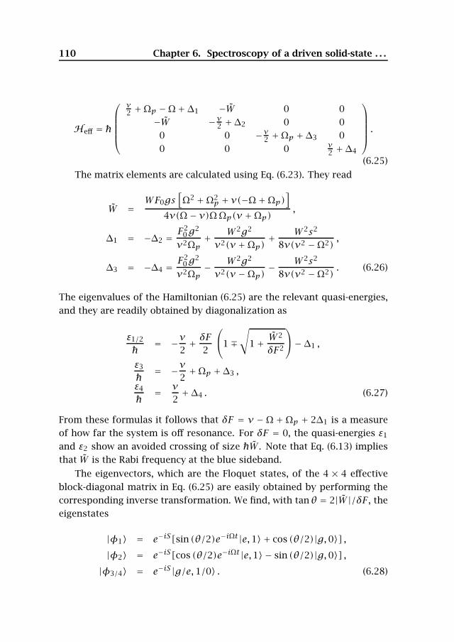
110 Chapter 6. Spectroscopy of a driven solid-state . . .
Heff =
⎛⎜⎜⎜⎜⎝
ν2 +Ωp −Ω+∆1 −W 0 0
−W −ν2 +∆2 0 00 0 −ν2 +Ωp +∆3 00 0 0 ν
2 +∆4
⎞⎟⎟⎟⎟⎠ .
(6.25)
The matrix elements are calculated using Eq. (6.23). They read
W =WF0gs
[Ω2 +Ω2
p + ν(−Ω +Ωp)]
4ν(Ω − ν)ΩΩp(ν +Ωp),
∆1 = −∆2 =F2
0g2
ν2Ωp+ W 2g2
ν2(ν +Ωp)+ W 2s2
8ν(ν2 −Ω2),
∆3 = −∆4 =F2
0g2
ν2Ωp− W 2g2
ν2(ν −Ωp)− W 2s2
8ν(ν2 −Ω2). (6.26)
The eigenvalues of the Hamiltonian (6.25) are the relevant quasi-energies,and they are readily obtained by diagonalization as
ε1/2
= −ν
2+ δF
2
⎛⎝1∓
√1+ W
2
δF2
⎞⎠−∆1 ,
ε3
= −ν
2+Ωp +∆3 ,
ε4
= ν
2+∆4 . (6.27)
From these formulas it follows that δF = ν −Ω +Ωp + 2∆1 is a measureof how far the system is off resonance. For δF = 0, the quasi-energies ε1
and ε2 show an avoided crossing of size W . Note that Eq. (6.13) impliesthat W is the Rabi frequency at the blue sideband.
The eigenvectors, which are the Floquet states, of the 4 × 4 effectiveblock-diagonal matrix in Eq. (6.25) are easily obtained by performing thecorresponding inverse transformation. We find, with tanθ = 2|W |/δF , theeigenstates
|φ1〉 = e−iS[sin (θ/2)e−iΩt|e,1〉 + cos (θ/2)|g,0〉] ,|φ2〉 = e−iS[cos (θ/2)e−iΩt|e,1〉 − sin (θ/2)|g,0〉] ,
|φ3/4〉 = e−iS|g/e, 1/0〉 . (6.28)
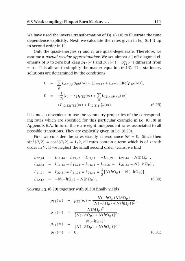
6.3 Weak coupling: Floquet-Born-Markov . . . 111
We have used the inverse transformation of Eq. (6.10) to illustrate the timedependence explicitly. Next, we calculate the rates given in Eq. (6.14) upto second order in V .
Only the quasi-energies ε1 and ε2 are quasi-degenerate. Therefore, weassume a partial secular approximation: We set almost all off-diagonal el-ements of ρ to zero but keep ρ12(∞) and ρ21(∞) = ρ∗12(∞) different fromzero. This allows to simplify the master equation (6.13). The stationarysolutions are determined by the conditions
0 =∑βLαα,ββρββ(∞)+ (Lαα,12 + Lαα,21)Re[ρ12(∞)],
0 = − i(ε1 − ε2)ρ12(∞)+
∑αL12,ααραα(∞)
+L12,12ρ12(∞)+ L12,21ρ∗12(∞). (6.29)
It is most convenient to use the symmetry properties of the correspond-ing rates which are specified for this particular example in Eq. (6.58) inAppendix 6.A. In turn, there are eight independent rates associated to allpossible transitions. They are explicitly given in Eq. (6.59).
First we consider the rates exactly at resonance δF = 0. Since thensin2(θ/2) = cos2(θ/2) = 1/2, all rates contain a term which is of zerothorder in V . If we neglect the small second order terms, we find
L22,44 = L11,44 = L33,22 = L33,11 = −L33,21 = L21,44 = N(Ωp) ,L22,33 = L11,33 = L44,22 = L44,11 = L44,21 = −L21,33 = N(−Ωp) ,
L11,21 = L22,21 = L21,22 = L21,11 = 12[N(Ωp)−N(−Ωp)] ,
L12,12 = −N(−Ωp)−N(Ωp) . (6.30)
Solving Eq. (6.29) together with (6.30) finally yields
ρ11(∞) = ρ22(∞) =N(−Ωp)N(Ωp)
[N(−Ωp)+N(Ωp)]2,
ρ33(∞) = N(Ωp)2
[N(−Ωp)+N(Ωp)]2,
ρ44(∞) = N(−Ωp)2[N(−Ωp)+N(Ωp)]2
,
ρ12(∞) = 0 . (6.31)
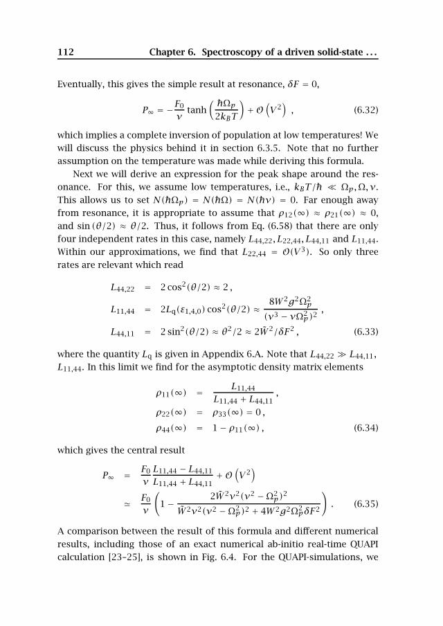
112 Chapter 6. Spectroscopy of a driven solid-state . . .
Eventually, this gives the simple result at resonance, δF = 0,
P∞ = −F0
νtanh
(Ωp2kBT
)+O
(V 2), (6.32)
which implies a complete inversion of population at low temperatures! Wewill discuss the physics behind it in section 6.3.5. Note that no furtherassumption on the temperature was made while deriving this formula.
Next we will derive an expression for the peak shape around the res-onance. For this, we assume low temperatures, i.e., kBT/ Ωp,Ω, ν.This allows us to set N(Ωp) = N(Ω) = N(ν) = 0. Far enough awayfrom resonance, it is appropriate to assume that ρ12(∞) ≈ ρ21(∞) ≈ 0,and sin (θ/2) ≈ θ/2. Thus, it follows from Eq. (6.58) that there are onlyfour independent rates in this case, namely L44,22, L22,44, L44,11 and L11,44.Within our approximations, we find that L22,44 = O(V 3). So only threerates are relevant which read
L44,22 = 2 cos2(θ/2) ≈ 2 ,
L11,44 = 2Lq(ε1,4,0) cos2(θ/2) ≈8W 2g2Ω2
p
(ν3 − νΩ2p)2
,
L44,11 = 2 sin2(θ/2) ≈ θ2/2 ≈ 2W 2/δF2 , (6.33)
where the quantity Lq is given in Appendix 6.A. Note that L44,22 L44,11,L11,44. In this limit we find for the asymptotic density matrix elements
ρ11(∞) = L11,44
L11,44 + L44,11,
ρ22(∞) = ρ33(∞) = 0 ,
ρ44(∞) = 1− ρ11(∞) , (6.34)
which gives the central result
P∞ = F0
νL11,44 − L44,11
L11,44 + L44,11+O
(V 2)
F0
ν
(1−
2W 2ν2(ν2 −Ω2p)2
W 2ν2(ν2 −Ω2p)2 + 4W 2g2Ω2
pδF2
). (6.35)
A comparison between the result of this formula and different numericalresults, including those of an exact numerical ab-initio real-time QUAPIcalculation [23–25], is shown in Fig. 6.4. For the QUAPI-simulations, we
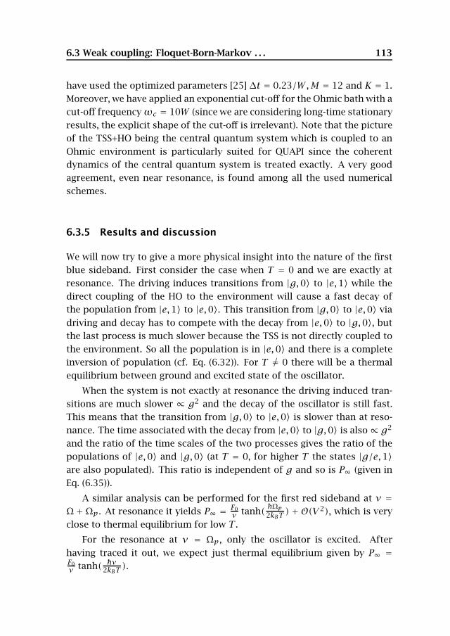
6.3 Weak coupling: Floquet-Born-Markov . . . 113
have used the optimized parameters [25] ∆t = 0.23/W,M = 12 and K = 1.Moreover, we have applied an exponential cut-off for the Ohmic bath with acut-off frequencyωc = 10W (since we are considering long-time stationaryresults, the explicit shape of the cut-off is irrelevant). Note that the pictureof the TSS+HO being the central quantum system which is coupled to anOhmic environment is particularly suited for QUAPI since the coherentdynamics of the central quantum system is treated exactly. A very goodagreement, even near resonance, is found among all the used numericalschemes.
6.3.5 Results and discussion
We will now try to give a more physical insight into the nature of the firstblue sideband. First consider the case when T = 0 and we are exactly atresonance. The driving induces transitions from |g,0〉 to |e,1〉 while thedirect coupling of the HO to the environment will cause a fast decay ofthe population from |e,1〉 to |e,0〉. This transition from |g,0〉 to |e,0〉 viadriving and decay has to compete with the decay from |e,0〉 to |g,0〉, butthe last process is much slower because the TSS is not directly coupled tothe environment. So all the population is in |e,0〉 and there is a completeinversion of population (cf. Eq. (6.32)). For T = 0 there will be a thermalequilibrium between ground and excited state of the oscillator.
When the system is not exactly at resonance the driving induced tran-sitions are much slower ∝ g2 and the decay of the oscillator is still fast.This means that the transition from |g,0〉 to |e,0〉 is slower than at reso-nance. The time associated with the decay from |e,0〉 to |g,0〉 is also∝ g2
and the ratio of the time scales of the two processes gives the ratio of thepopulations of |e,0〉 and |g,0〉 (at T = 0, for higher T the states |g/e, 1〉are also populated). This ratio is independent of g and so is P∞ (given inEq. (6.35)).
A similar analysis can be performed for the first red sideband at ν =Ω +Ωp. At resonance it yields P∞ = F0
ν tanh( Ωp2kBT ) +O(V 2), which is veryclose to thermal equilibrium for low T .
For the resonance at ν = Ωp, only the oscillator is excited. Afterhaving traced it out, we expect just thermal equilibrium given by P∞ =F0ν tanh( ν
2kBT ).
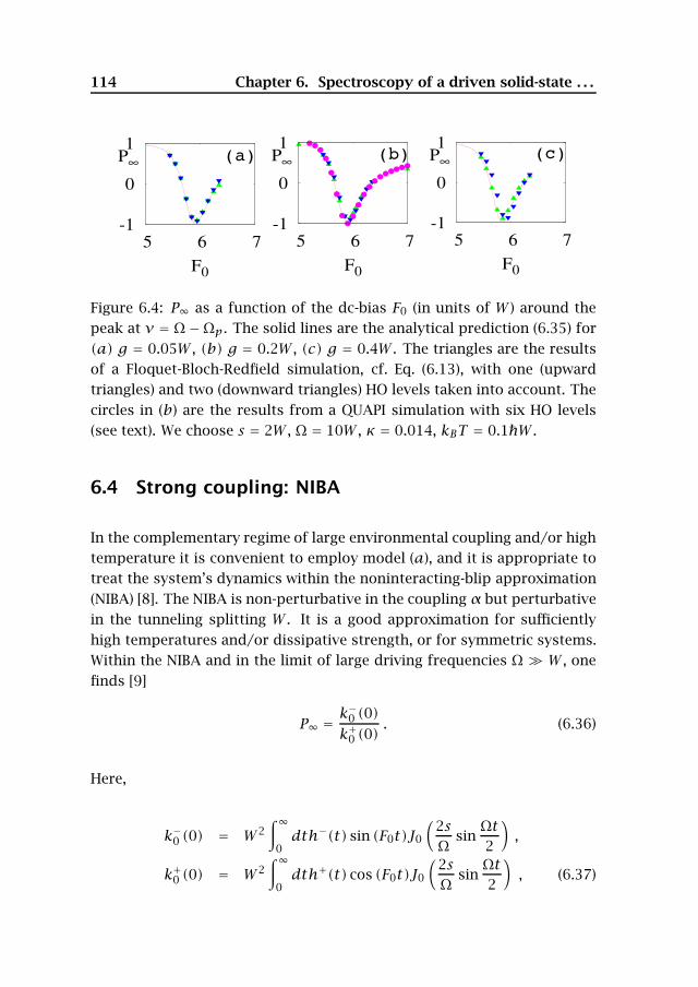
114 Chapter 6. Spectroscopy of a driven solid-state . . .
(b) (c)
-1
0
1
5 6 7
F0
P∞
-1
0
1
5 6 7
F0
P∞
-1
0
1
5 6 7
F0
P∞(a)
Figure 6.4: P∞ as a function of the dc-bias F0 (in units of W ) around thepeak at ν = Ω −Ωp. The solid lines are the analytical prediction (6.35) for(a) g = 0.05W , (b) g = 0.2W , (c) g = 0.4W . The triangles are the resultsof a Floquet-Bloch-Redfield simulation, cf. Eq. (6.13), with one (upwardtriangles) and two (downward triangles) HO levels taken into account. Thecircles in (b) are the results from a QUAPI simulation with six HO levels(see text). We choose s = 2W , Ω = 10W , κ = 0.014, kBT = 0.1W .
6.4 Strong coupling: NIBA
In the complementary regime of large environmental coupling and/or hightemperature it is convenient to employ model (a), and it is appropriate totreat the system’s dynamics within the noninteracting-blip approximation(NIBA) [8]. The NIBA is non-perturbative in the coupling α but perturbativein the tunneling splitting W . It is a good approximation for sufficientlyhigh temperatures and/or dissipative strength, or for symmetric systems.Within the NIBA and in the limit of large driving frequencies Ω W , onefinds [9]
P∞ =k−0 (0)k+0 (0)
. (6.36)
Here,
k−0 (0) = W 2∫∞
0dth−(t) sin (F0t)J0
(2sΩ
sinΩt2
),
k+0 (0) = W 2∫∞
0dth+(t) cos (F0t)J0
(2sΩ
sinΩt2
), (6.37)
6.4 Strong coupling: NIBA 115
with J0 being the zeroth order Bessel function. Dissipative effects of theenvironment are captured by the terms
h+(t) = e−Q′(t) cos[Q′′(t)] ,
h−(t) = e−Q′(t) sin[Q′′(t)] . (6.38)
Here, Q′(t) and Q′′(t) are the real and imaginary parts of the bath corre-lation function
Q(t) =∫∞
0dω
J(ω)ω2
cosh(ωβ/2)− cosh[ω(β/2− it)]sinh(ωβ/2)
.
For the peaked spectral density given in Eq. (6.4) one finds
Q′(t) = Q′1(t)− e−Γt[Y1 cos(Ωpt)+ Y2 sin(Ωpt)] ,
Q′′(t) = A1 − e−Γt[A1 cos(Ωpt)+A2 sin(Ωpt)] . (6.39)
Here, β = /kBT , Γ = πκΩp , Ω2p = Ω2
p − Γ2 and
Q′1(t) = Y1 +παΩ2p
[sinh(βΩp)t
2CΩp+ sin(βΓ)t
2CΓ
−4Ω2
p
β
∞∑n=1
1νn [e
−νnt − 1]+ t(Ω2p + ν2
n)2 − 4Γ2ν2n
⎤⎦ , (6.40)
where νn = 2πn/β. Moreover, C = cosh(βΩp) − cos(βΓ), A2 = απ(Γ2 −Ω2p)/(2Γ Ωp), A1 = πα, CY1/2 = ∓A2/1 sinh (βΩp) − A1/2 sin (βΓ) . As
follows from Eq. (6.39), Q′ and Q′′ display damped oscillations with fre-quency Ωp (cf. Fig. 6.5b) which are not present for a pure Ohmic spectrum.It is the interplay between these oscillations and the driving field which in-duces the extra resonances in P∞.
To proceed, we rewrite the kernels k±0 (0) in a more convenient form.In the integrand of Eq. (6.37) the functions cos[Q′′(t)], sin[Q′′(t)] ande−Q′(t)+Q
′1(t) oscillate with frequency Ωp and we can expand them as
cos[Q′′(t)] =∞∑
m=−∞
[Dm cos(mΩpt)+ Em sin(mΩpt)
],
sin[Q′′(t)] =∞∑
m=−∞
[Fm cos(mΩpt)+Gm sin(mΩpt)
],
e−Q′(t)+Q′1(t) =
∞∑m=−∞
[Hm cos(mΩpt)+ Km sin(mΩpt)
].
(6.41)
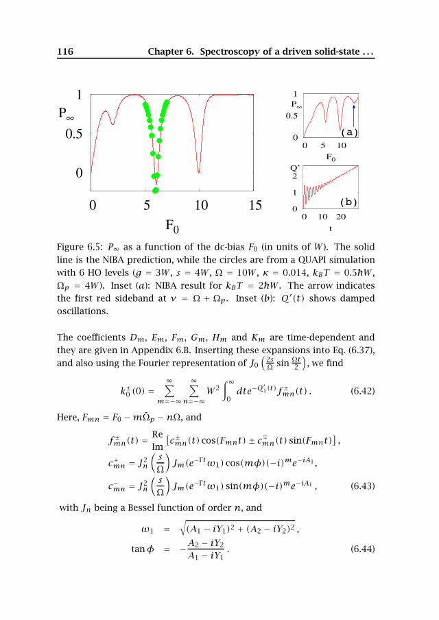
116 Chapter 6. Spectroscopy of a driven solid-state . . .
0
0.5
1
0 5 10 15
F0
P∞
0
0.5
1
0 5 10
F0
P∞
0
1
2
0 10 20
t
Q’
(a)
(b)
Figure 6.5: P∞ as a function of the dc-bias F0 (in units of W ). The solidline is the NIBA prediction, while the circles are from a QUAPI simulationwith 6 HO levels (g = 3W , s = 4W , Ω = 10W , κ = 0.014, kBT = 0.5W ,Ωp = 4W ). Inset (a): NIBA result for kBT = 2W . The arrow indicatesthe first red sideband at ν = Ω + Ωp. Inset (b): Q′(t) shows dampedoscillations.
The coefficients Dm, Em, Fm, Gm, Hm and Km are time-dependent andthey are given in Appendix 6.B. Inserting these expansions into Eq. (6.37),and also using the Fourier representation of J0
(2sΩ sin Ωt
2
), we find
k±0 (0) =∞∑
m=−∞
∞∑n=−∞
W 2∫∞
0dte−Q
′1(t)f±mn(t) . (6.42)
Here, Fmn = F0 −mΩp −nΩ, and
f±mn(t) =ReIm
[c±mn(t) cos(Fmnt)± c∓mn(t) sin(Fmnt)
],
c+mn = J2n
( sΩ
)Jm(e−Γtω1) cos(mφ)(−i)me−iA1 ,
c−mn = J2n
( sΩ
)Jm(e−Γtω1) sin(mφ)(−i)me−iA1 , (6.43)
with Jn being a Bessel function of order n, and
ω1 =√(A1 − iY1)2 + (A2 − iY2)2 ,
tanφ = −A2 − iY2
A1 − iY1. (6.44)
6.5 Limit Ωp ν 117
Thus, from Eq. (6.43), we expect resonances when Fnm = 0.In the limit Γ/Ωp 1 and for not too large T (i.e., cos(βΓ) cosh(βΩp)),
we find that
tan(mφ) ≈ i tanh
(mβΩp
2
). (6.45)
Inserting this into Eq. (6.43), we obtain
i tanh
(mβΩp
2
)c+mn = c−mn . (6.46)
If the environmental mode is enough localized (i.e., the integrand of Eq.(6.37) is only damped after several oscillations), we expect that the sum inEq. (6.42) is dominated by the coefficient of cos (Fnmt) if Fmn = 0. Thismeans that
f+mn(t) ≈ Re[c+mn(t)]
f−mn(t) ≈ tanh
(mβΩp
2
)Re[c+mn(t)] , (6.47)
which leads to
P∞ = tanh
(mβΩp
2
). (6.48)
Without driving we only have terms with n = 0, and Fm0 = 0 impliesthat F0 =mΩp. In that case Eq. (6.48) gives the NIBA thermal equilibriumvalue. Hence, in order to find resonances we need to apply driving. For“conventional” resonances at F0 = nΩ, we putm to zero and we find P∞ ≈0, as predicted for unstructured environments [17, 26]. Finally, for F0 =nΩ ±mΩp, we recover P∞ ≈ ± tanh(mβΩp/2), as was also found withinthe Floquet-Born-Markov approach, cf. Eq. (6.32). Results of a numericalevaluation of P∞ are shown in Fig. 6.5, using the NIBA result (6.43), as wellas the exact ab-initio real-time QUAPI method [23–25]. Resonance dips areobserved at F0 = Ω, F0 = Ω − Ωp and F0 = Ω − 2Ωp . For kBT ∼ Ωp, wealso find the first red sideband at F0 = Ω +Ωp, see inset (a).
6.5 Limit Ωp ν
In the limit when the frequency Ωp of the HO is much larger than the ef-fective TSS level splitting ν, the peak in the spectral density at Ωp acts as
118 Chapter 6. Spectroscopy of a driven solid-state . . .
a high-frequency cut-off for an effective Ohmic bath, see Eq. (6.4). In otherwords, the oscillations in the correlation functions, see Sec. 6.4 which oc-cur on a time-scale Ω−1
p are very fast and can be averaged out when onlythe long-time dynamics is of interest and short-time effects are not con-sidered. In this limit, the standard driven and Ohmically damped spin-boson model [8, 9] is recovered. In the regime of weak damping α 1,the stationary population difference P∞ has been determined within theassumption of large driving frequencies (Ω W,ν and Ω much largerthan the decay rate) upon using analytic real-time path integral methodsin Ref. [26]. In this Section, we use this high-frequency approximation ofRef. [26] as a starting point, and derive a closed simple analytic expres-sion for the peak shape of the “common” multi-photon resonance. Mostimportantly, we find the scaling of the width of the n-photon resonance asthe n-th Bessel function Jn(s/Ω). This scaling behavior has been observedexperimentally in superconducting flux qubit devices [16].
The central issue in finding a closed analytic expression for P∞ is tofind the roots ϑn of the pole equation [26]
+∞∏n=−∞
(F2n − ϑ2
)++∞∑n=0
W 2n
+∞∏m=−∞,m =n
(F2m − ϑ2
)= 0 . (6.49)
Here, Fn = F0 − nΩ is the photon-induced bias and Wn = |Jn(s/Ω)|W isthe field-dressed tunneling splitting of the TSS, where Jn(x) is the n-thordinary Bessel function. Considering the n-photon resonance, we numer-ically find that, up to extremely high numerical precision, the roots of Eq.(6.49) are given by
ϑ0 =√F2
0 +W 20 ,
ϑn=0 =√F2n +W 2
n ,
ϑk=n,0 = Fk . (6.50)
Plugging Eqs. (6.50) in the expressions for P∞ given in Ref. [26], see Eqs.(6) and (7) therein, we find the closed expression for the lineshape of then-photon resonance to be
6.5 Limit Ωp ν 119
P(n)∞ (F0) =F0F2
nW20 (F
20 +W 2
0 − F2n)JOhm(ϑ0)ϑ0
+ F20 |Fn|W 2
n(F2n +W 2
n − F20 )JOhm(ϑn)ϑn
Z0n + Zn0(6.51)
Zij = W 2i F
2j (F
2i +W 2
i − F2j )JOhm(ϑi) coth
ϑi2kBT
. (6.52)
This result can be simplified upon observing that the second term inthe numerator is small if the driving is not too large, since then W 2
n W 20 .
Moreover, we are interested in the regime F0 W which is the saturationregime implying that ν ≈ F0 and in low temperatures. Then, away fromthe resonance point at nΩ ≈ F0, the second term in the denominator in Eq.(6.52) can be neglected and one recovers the standard result, if one usesthat W0 ≈ W which is fulfilled for weak driving. It reads
P(n)∞ (F0) = F0√F2
0 +W 2tanh
√F2
0 +W 2
2kBT, (6.53)
which gives the correct result away from any n-photon resonance. For thecase at the n-photon resonance at nΩ ≈ F0, one finds a Lorentzian lineshape, i.e.,
P(n)∞ (F0) =W 2
0 (F0 −nΩ)2W 2
0 (F0 −nΩ)2 + 2F20W
2nkBT/
, (6.54)
where we have expanded the second coth term in the denominator (see Eq.(6.52)) up to lowest order in the argument, which is appropriate since ϑn issmall at resonance. The linewidth of the Lorentzian peak can be calculatedas the full width at half maximum (FWHM)
∆F(n) = 2
√√√√2nΩ(WnW0
)2 kBT
+(WnW0
)4 (kBT
)2
. (6.55)
Note that this result obtained from the high-frequency approximation isindependent of the damping constant. Moreover, the leading term is thefirst term under the square root in Eq. (6.55). Note furthermore that forthe case of infinitesimal driving, the FWHM is not correctly reproduced byEq. (6.55) since it would approach zero. However, as it is known from NMR
120 Chapter 6. Spectroscopy of a driven solid-state . . .
within a treatment in terms of the Bloch equation, in this case, the FWHMis dominated by the dephasing [17], i.e.,
∆F(1)Bloch = 2√Γ2φ +Ω2
RΓφ/ΓR , (6.56)
where ΓR = πα coth(ν/2kBT)W 2/ν is the relaxation rate and Γφ = ΓR/2+2πα(F2
0 /ν2)kBT/ [8]. Both rates are of first order in the damping strengthα. Moreover, ΩR is the (single-photon) Rabi frequency. Hence, we have toinclude the dephasing rate Γ2
φ in Eq. (6.54), since it cannot be reproducedby our weak-coupling approach which is only of first order in α. Thisfinally yields in leading order in the driving strength
∆F(n) = 2
√√√Γ2φ +
(WnW0
)2
2nΩkBT. (6.57)
As follows from Eq. (6.57), the FWHM of the n-photon resonance scaleswith the n-th ordinary Bessel function, i.e., ∆F(n) ∼ Jn(s/Ω) as also con-firmed by experiments [16].
6.6 Conclusions
In conclusion we have investigated the problem of a quantum mechanicaldriven two-state system being coupled to a structured environment whichhas a localized mode at a frequency Ωp but behaves Ohmically at lowfrequencies. We have studied two complementary parameter regimes ofweak and strong coupling to the environment. The interplay of the drivingand the localized mode gives additional features like resonant peaks/dipsin the asymptotic averaged population difference P∞. We have calculatedanalytically the lineshape of the resonances in various parameter regimesand have obtained simple closed expressions for the particular example ofthe first blue sideband. We also include the discussion of how the resultsare generalized for any sideband. Moreover, we have elaborated the limitwhen the localized mode acts as a high-frequency cut-off. Then, the fullwidth at half maximum of the n-photon resonance has been shown toscale with the n-th ordinary Bessel function.
Our model finds as well applications in the field of cavity quantum elec-trodynamics (CQED) with solid state structures [27]. Most interestingly,
6. Symmetry properties for the dissipative rates . . . 121
the strong coupling limit of CQED could be reached in superconductingelectrical circuits, with perspective applications ahead.
Finally, we note that a related experiment has been reported recentlyby Wallraff et al. [28]. There, a qubit was realized in the form of a Cooperpair box which couples to a single mode of a cavity which is damped. Theproperties of the TSS-HO were probed spectroscopically by measuring thetransmission of the resonator. In other words, a driven HO was consideredwhile the TSS was kept static. In contrast to that system, here, the TSS wastime-dependent while the HO is treated as static.
6.A Symmetry properties for the dissipative rates for
the first blue sideband
In order to evaluate the stationary averaged population difference P∞, therate coefficients Lαβ,α′β′ have to be determined explicitly. For the exampleof the resonance at ν ≈ Ω − Ωp (first blue sideband) considered in thiswork, we find that the rate coefficients fulfill the symmetry relations
L11,22 = L22,11 = L33,44 = L44,33 = 0, L11,11 = −(L33,11 + L44,11),L22,22 = −(L33,22 + L44,22), L33,33 = −(L11,33 + L44,33),L44,44 = −(L11,44 + L22,44), L12,12 = (L22,22 + L11,11)/2,L11,33 = L44,22, L22,33 = L44,11, L33,22 = L11,44,L33,11 = L22,44, L22,21 = L21,11, L11,21 = L21,22,L44,21 = −L21,33, L33,21 = −L21,44, L22,12 = L22,21,L11,12 = L11,21, L44,12 = L44,21, L33,21 = L33,12,L12,21 = 0.
(6.58)
122 Chapter 6. Spectroscopy of a driven solid-state . . .
As a consequence, there are eight independent rates given by
L44,22 = 2Losc(ε4,2,−1) cos2(θ2
)+ 2Lq(ε4,2,0) sin2
(θ2
)−Lq,osc(ε4,2,−1) sinθ ,
L22,44 = 2Losc(ε2,4,1) cos2(θ2
)+ 2Lq(ε2,4,0) sin2
(θ2
)−Lq,osc(ε2,4,1) sinθ ,
L44,11 = 2Losc(ε4,1,−1) sin2(θ2
)+ 2Lq(ε4,1,0) cos2
(θ2
)+Lq,osc(ε4,1,−1) sinθ ,
L11,44 = 2Losc(ε1,4,1) sin2(θ2
)+ 2Lq(ε1,4,0) cos2
(θ2
)+Lq,osc(ε1,4,1) sinθ ,
L21,22 = 12
(Losc(ε3,2,0)− Lq(ε3,2,−1)− Losc(ε4,2,−1)+ Lq(ε4,2,0)
)sinθ
+12(Lq,osc(ε3,2,0)− Lq,osc(ε4,2,−1)) cosθ ,
L21,11 = 12
(Losc(ε3,1,0)− Lq(ε3,1,−1)− Losc(ε4,1,−1)+ Lq(ε4,1,0)
)sinθ
+12(Lq,osc(ε3,1,0)− Lq,osc(ε4,1,−1)) cosθ ,
L21,44 = 12
(Losc(ε1,4,1)+ Losc(ε2,4,1)− Lq(ε1,4,0)− Lq(ε2,4,0)
)sinθ
+12(Lq,osc(ε1,4,1)+ Lq,osc(ε2,4,1)) cosθ ,
L21,33 = 12
(Lq(ε1,3,1)+ Lq(ε2,3,1)− Losc(ε1,3,0)− Losc(ε2,3,0)
)sinθ
−12(Lq,osc(ε1,3,0)+ Lq,osc(ε2,3,0)) cosθ ,
with
Lq(εklm) = 〈e,1,0|eiSXe−iS |g,1,0〉2N(εklm)= 〈e,0,0|eiSXe−iS |g,0,0〉2N(εklm)
=4g2W 2Ω2
pN(εklm)
ν2(ν2 −Ω2p)2
,
Losc(εklm) = 〈g,1,0|eiSXe−iS |g,0,0〉2N(εklm)= 〈e,1,0|eiSXe−iS |e,0,0〉2N(εklm)
=(
4g2(W 2(ν2 − 2Ω2p)− (ν2 −Ω2
p)2)Ω2p(ν2 −Ω2
p)2+ 1
)N(εklm) ,
Lq,osc(εklm)N(εklm)
= −2〈e,1,−1|eiSXe−iS|g,1,0〉〈g,1,0|eiSXe−iS |g,0,0〉
= 2〈g,0,1|eiSXe−iS|e,0,0〉〈e,0,0|eiSXe−iS |e,1,0〉
= WF0gs((Ω +Ωp)2 + 2Ω2p + ν(−Ω +Ωp))
2ν(ν −Ω)Ω(ν −Ω−Ωp)Ωp(ν +Ωp),
N(εklm) = N(εk − εl +mΩ) . (6.59)
Note that Losc is the rate containing the zeroth order term in g and s. Itis related to the transition between two states differing by one oscillator
6.B Coefficients for the kernels k±0 (0) 123
quantum. This decay is of zeroth order (hence fast) because the oscillatoris coupled directly to the environment. Moreover, Lq gives the rate fortransitions between the excited and ground state of the TSS with the HOremaining in the same state, and Lq,osc is related to the transition whereboth the qubit and the oscillator exchange energy with the environment.Note that this transition is induced by the driving and involves one photon.
6.B Coefficients for the kernels k±0 (0)
In Sec. 6.4, we have introduced an expansion of the oscillating functionsgiven in Eq. (6.41). In this appendix we summarize the correspondingcoefficients for completeness.
For the expansion of cos[Q′′(t)], we find
D2m+1 = (−1)m sin (A1)J2m+1(A) cos [(2m+ 1)X] ,
D2m = (−1)m cos (A1)J2m(A) cos (2mX) ,
E2m+1 = (−1)m sin (A1)J2m+1(A) sin [(2m+ 1)X] ,
E2m = (−1)m cos (A1)J2m(A) sin (2mX), (6.60)
where we have introduced
A = e−Γt√A2
1 +A22 ,
sinX = A2/√A2
1 +A22 . (6.61)
In the same way, the expansion of sin[Q′′(t)] gives
F2m+1 = (−1)m+1 cos (A1)J2m+1(A) cos [(2m+ 1)X] ,
F2m = (−1)m sin (A1)J2m(A) cos [2mX],
G2m+1 = (−1)m+1 cos (A1)J2m+1(A) sin ([2m+ 1)X] ,
G2m = (−1)m sin (A1)J2m(A) sin [2mX] . (6.62)
Finally, we find for the coefficients of exp[Q(t)−Q1(t)]
Hm = Im(Y) cos (mV) ,
Km = Im(Y) sin (mV) , (6.63)
124 Chapter 6. Spectroscopy of a driven solid-state . . .
where we have introduced
Y = e−Γt√Y 2
1 + Y 22 ,
tanV = Y2
Y1. (6.64)
Here, Im is the modified Bessel function of the first kind of orderm.
Bibliography
[1] Y. Nakamura, Yu. A. Pashkin, and J. S. Tsai, Nature 398, 786 (1999).
[2] J. M. Martinis, S. Nam, J. Aumentado, and C. Urbina, Phys. Rev. Lett.89, 117901 (2002).
[3] Yu. A. Pashkin, T. Yamamoto, O. Astafiev, Y. Nakamura, D. V. Averin,and J. S. Tsai, Nature 421, 823 (2003).
[4] D. Vion, A. Aassime, A. Cottet, P. Joyez, H. Pothier, C. Urbina, D. Es-teve, and M. H. Devoret, Science 296, 886 (2002).
[5] I. Chiorescu, Y. Nakamura, C. J. P. M. Harmans, and J. E. Mooij, Science299, 1869 (2003).
[6] I. Chiorescu, P. Bertet, K. Semba, Y. Nakamura, C. J. P. M. Harmans,and J. E. Mooij, Nature 431, 159 (2004).
[7] C. Cohen-Tannoudji, J. Dupont-Roc and G. Grynberg, Atom-Photon In-teractions (Wiley, New York, 1992).
[8] U. Weiss, Quantum Dissipative Systems (World Scientific, Singapore,1999).
[9] M. Grifoni and P. Hanggi, Phys. Rep. 304, 229 (1998).
[10] L. Tian, S. Lloyd, and T.P. Orlando, Phys. Rev. B 65, 144516 (2002).
[11] M. Thorwart, L. Hartmann, I. Goychuk, and P. Hanggi, J. Mod. Opt. 47,2905 (2000).
[12] A. Yu. Smirnov, Phys. Rev. B 67, 155104 (2003).
126 Bibliography
[13] M. Thorwart, E. Paladino and M. Grifoni, Chem. Phys. 296, 333 (2004).
[14] F. K. Wilhelm, S. Kleff and J. von Delft, Chem. Phys. 296, 345 (2004).
[15] S. Kleff, S. Kehrein, and J. von Delft, Phys. Rev. B 70, 014516 (2004).
[16] S. Saito, M. Thorwart, H. Tanaka, M. Ueda, H. Nakano, K. Semba, andH. Takayanagi, Phys. Rev. Lett. 93, 037001 (2004).
[17] M. C. Goorden and F. K. Wilhelm, Phys. Rev. B 68, 012508 (2003).
[18] A. Garg, J. N. Onuchic and V. Ambegaokar, J. Chem. Phys. 83, 4491(1985).
[19] R. Blumel, R. Graham, L. Sirko, U. Smilansky, H. Walther, and K. Ya-mada, Phys. Rev. Lett. 62, 341 (1989).
[20] S. Kohler, T. Dittrich, and P. Hanggi, Phys. Rev. E 55, 300 (1997).
[21] J.H. Shirley, Phys. Rev. 138, B979 (1965).
[22] I. Shavit and L. T. Redmon, J. Chem. Phys. 73, 5711 (1980).
[23] N. Makri and D.E. Makarov, J. Chem. Phys. 102, 4600 (1995).
[24] M. Thorwart, P. Reimann, P. Jung, and R. F. Fox, Chem. Phys. 235, 61(1998).
[25] M. Thorwart, P. Reimann, and P. Hanggi, Phys. Rev. E 62, 5808 (2000).
[26] L. Hartmann, I. Goychuk, M. Grifoni, and P. Hanggi, Phys. Rev. E 61,R4687 (2000).
[27] S. M. Girvin, R.-S. Huang, A. Blais, A. Wallraff, and R. J. Schoelkopf,in Proceedings of Les Houches Summer School, Session LXXIX, Quan-tum Entanglement and Information Processing (2003); see also cond-mat/0310670.
[28] A. Wallraff, D. I. Schuster, A. Blais, L. Frunzio, R.-S. Huang, J. Majer, S.Kumar, S. M. Girvin, and R. J. Schoelkopf, Nature 431, 162 (2004).
Samenvatting
Andreevreflectie vindt plaats aan het grensvlak tussen een normaal me-taal en een supergeleider. Bij dit bijzondere reflectiemechanisme wordteen elektron gereflecteerd als een gat. Wanneer het elektron op het Fer-miniveau is, keert het gat precies terug langs het pad van het elektron.Andreevreflectie speelt een belangrijke rol in een Andreevbiljart. Een An-dreevbiljart bestaat uit een zogenaamde “quantum dot” die via een quan-tumpuntcontact gekoppeld is aan een supergeleider. De quantum dot zelfis te vergelijken met een biljart, gemaakt in een tweedimensionaal elek-tronengas. Aangezien er in de quantum dot geen verontreinigingen zijn,vindt alle reflectie plaats aan de wanden. Wij beschouwen quantum dotsmet een zodanige vorm dat de klassieke beweging van een elektron (of gat)in de dot chaotisch is.
De beweging van elektronen en gaten in een Andreevbiljart wordt be-schreven door de quantummechanica. Volgens de stelling van Ehrenfestis de beweging aanvankelijk langs een klassiek pad. Naarmate de tijd vor-dert zijn de positie en de snelheid steeds minder goed gedefinieerd. Naeen bepaalde tijd is de onzekerheid in de positie van het elektron of gateven groot als de afmeting van het Andreevbiljart. Dit is de EhrenfesttijdτE . De Ehrenfesttijd karakteriseert de overgang van klassieke mechanicanaar quantummechanica.
Als de Ehrenfesttijd veel langer is dan de gemiddelde tijd τD tussenAndreevreflecties, is een beschrijving in termen van klassieke paden geoor-loofd. Andreevreflectie maakt alle paden (bij benadering) periodiek, dusquantisatie volgens de Bohr-Sommerfeld methode is mogelijk. In de te-genovergestelde limiet τE τD geeft toevalsmatrixtheorie een goede be-schrijving. Terwijl toevalsmatrixtheorie voorspelt dat de toestandsdicht-heid in een chaotisch Andreevbiljart identiek nul wordt voor lage ener-
128 Samenvatting
gieen (d.w.z. er ontstaat een “gat”), geeft quantisatie van periodieke padenslechts een geleidelijke afname van de toestandsdichtheid zonder een echt“gat”. In dit proefschrift wordt een nieuwe theorie gegeven die beide eer-dere theorieen met elkaar verbindt.
Het idee achter onze theorie is eenvoudig. We quantiseren alle klassie-ke paden met een verblijftijd T in de quantum dot, die korter is dan deEhrenfesttijd door middel van de Bohr-Sommerfeld methode. Het overigegedeelte van de faseruimte wordt gequantiseerd via toevalsmatrixtheoriemet effectieve parameters. De theorie wordt uitgewerkt in het tweede toten met het vijfde hoofdstuk.
Hoofdstuk twee vormt de basis voor de rest van het proefschrift. Vooreen beschrijving van de paden met T < τE is een precieze kennis van deklassieke beweging vereist. We beschouwen de beweging van een elektronmet een energie E boven het Ferminiveau. Het Andreev gereflecteerde gatkeert niet precies terug langs het pad van het elektron, daarom is het padniet precies gesloten maar drijft af in de faseruimte. We hebben gevon-den dat de tijd T tussen opeenvolgende Andreevreflecties een adiabatischbehouden grootheid is. Met deze kennis is het mogelijk een uitdrukkingte vinden voor de energieniveaus behorend bij de korte paden. Onze qua-siklassieke theorie is niet toepasbaar voor lange paden met T > τE . Wenemen aan dat het gedeelte van de faseruimte met lange paden kan wor-den beschreven door effectieve toevalsmatrixtheorie.
Een computersimulatie is een goede methode om onze theorie te tes-ten. Een zeer effectief model is de “Andreev kicked rotator”, dat eenstroboscopische beschrijving geeft van een Andreevbiljart. In het derdehoofdstuk gebruiken we dit stroboscopisch model om de fluctuaties vanhet laagste energie niveau te bepalen. De fluctuaties ontstaan omdat wede positie van de supergeleider veranderen. We vinden dat de amplitudevan de fluctuaties groeit met toenemende verhouding τE/τD . Effectievetoevalsmatrixtheorie geeft een goede beschrijving van de fluctuaties.
In hoofdstuk vier breiden we onze quasiklassieke theorie uit door detoevoeging van een zwak magneetveld, dat loodrecht op het Andreevbiljartstaat. De adiabatisch behouden grootheid van de klassieke beweging is nuniet meer de tijd T maar heeft ook een elektromagnetische component. Wevinden dat een magneetveld het laagste adiabatische niveau verlaagt meteen hoeveelheid die onafhankelijk is van de Ehrenfesttijd. Het magneet-veld veroorzaakt ook een afname van het laagste niveau van de effectieve
129
toevalsmatrixtheorie. Het gat in de toestandsdichtheid verdwijnt bij eenkritisch magneetveld dat afneemt met toenemende Ehrenfesttijd. Onzebevindingen komen goed overeen met computersimulaties.
In het vijfde hoofdstuk laten we zien dat onze theorie ook kan wordentoegepast op een quantum dot die niet gekoppeld is aan een supergeleider,maar aan twee elektronenreservoirs. Door dit systeem kan een stroom lo-pen. Omdat de stroom bestaat uit elektronen met een discrete lading, is erzelfs bij zeer lage temperaturen ruis. Deze zogenaamde hagelruis neemtaf met toenemende Ehrenfesttijd. Onze theorie voorspelt deze afname enis in staat deze te relateren aan de specifieke klassieke eigenschappen vaneen bepaald systeem.
Het zesde hoofdstuk behandelt een geheel ander systeem, de Joseph-son-junctie-qubit. De qubit bestaat uit een supergeleidende ring met drieJosephsonjuncties en kan in een superpositie zijn van een rechtsomdraai-ende en linksomdraaiende stroom. De qubit wordt gemeten door eenquantummechanisch meetinstrument, dat extra resonanties kan veroor-zaken. Dit is onlangs gemeten en wij geven een kwantitatieve beschrijvingvan het experiment.

130 Samenvatting
List of publications
• Optical imaging of contrast agent microbubbles in an ultrasound fieldwith a 100-MHz camera, N. de Jong, P. J. A. Frinking, A. Bouakaz, M.C. Goorden, T. Schuurmans, J. P. Xu, and F. Mastik, Ultrasound inMedicine and Biology 26, 487–492 (2000).
• Adiabatic quantization of Andreev quantum billiard levels, P. G. Sil-vestrov, M. C. Goorden, and C. W. J. Beenakker, Physical Review Let-ters 90, 116801 (2003). [Chapter 2]
• Noiseless scattering states in a chaotic cavity, P. G. Silvestrov, M. C.Goorden, and C. W. J. Beenakker, Physical Review B 67, 241301(R)(2003). [Chapter 5]
• Quasiclassical fluctuations of the superconductor proximity gap in achaotic system, M. C. Goorden, Ph. Jacquod, and C. W. J. Beenakker,Physical Review B 68, 220501(R) (2003). [Chapter 3]
• Theoretical analysis of continuously driven dissipative solid-state qu-bits, M. C. Goorden and F. K. Wilhelm, Physical Review B 68, 012508(2003).
• Entanglement spectroscopy of a driven solid-state qubit and its de-tector, M. C. Goorden, M. Thorwart, and M. Grifoni, Physical ReviewLetters 93, 267005 (2004).
• Spectroscopy of a driven solid-state qubit coupled to a structured en-vironment, M. C. Goorden, M. Thorwart, and M. Grifoni, EuropeanPhysical Journal B 45, 405 (2005). [Chapter 6]

132 List of publications
• Quantum-to-classical crossover for Andreev billiards in a magneticfield, M. C. Goorden, Ph. Jacquod, and C. W. J. Beenakker, to be pu-blished in Physical Review B. [Chapter 4]

Curriculum Vitæ
Ik ben geboren op 26 december 1976 te Sittard. Ik bezocht daar de Basis-school “Onder de Kastanje”. Ik genoot middelbaar onderwijs aan het Ger-trudislyceum in Roosendaal, waar ik in 1995 mijn VWO diploma behaalde.In datzelfde jaar begon ik met mijn studie Technische Natuurkunde aande TU Delft. In 2000 bracht ik een half jaar door bij NTT Basic ResearchLaboratories in Japan in de groep van Prof. dr. H. Takayanagi, waar ikexperimenteel werk deed op het gebied van Josephsonjunctie-qubits. In2002 studeerde ik af in de groep van Prof. dr. ir. J. E. Mooij, onder directebegeleiding van Dr. F. K. Wilhelm. De titel van mijn afstudeerscriptie is“Theory of Josephson persistent-current qubits with driving and dissipati-on”.
In april 2002 trad ik in dienst van de Stichting voor Fundamenteel On-derzoek der Materie als Onderzoeker in Opleiding. Ik deed mijn promotie-onderzoek aan het Instituut–Lorentz van het Leids Instituut voor Onder-zoek in de Natuurkunde aan de Universiteit Leiden in de groep van Prof.dr. C. W. J. Beenakker. De belangrijkste resultaten worden beschreven indit proefschrift. Tijdens mijn promotie heb ik geassisteerd bij de collegesStatistische Fysica I en Statistische en Thermische Fysica II. Tijdens mijnaanstelling presenteerde ik mijn werk in Mallorca, Geneve, Regensburg enDelft. Daarnaast woonde ik conferenties bij in Bad Honnef en Delft enbezocht ik een zomerschool in Wittenberg.
Per september 2005 zal ik werkzaam zijn als postdoc in de groep vanProf. dr. M. Buttiker aan de universiteit van Geneve.

134 Curriculum Vitæ
Dankwoord
Ik kijk met veel plezier terug op mijn tijd aan het Instituut–Lorentz. Ikhad het genoegen samen te werken met veel verschillende mensen, zowelbinnen als buiten het instituut. Peter het werk in mijn eerste jaar met joulegde de basis voor mijn proefschrift, Philippe en Milena: bedankt voorde gastvrijheid in Geneve en Regensburg. Ook buiten het werk was deatmosfeer op het instituut erg goed, ik kijk met veel plezier terug op degezamenlijke koffiepauzes en lunches en de jaarlijkse instituutsuitjes.
Daarnaast wil ik familie en vrienden bedanken voor alle steun en aflei-ding de afgelopen jaren. Noor en Eelke, bedankt dat jullie mijn paranymp-hen willen zijn. En tot slot, Herman ik jou ook . . .

Stellingenbehorende bij het proefschrift
On Superconductivity in nanostructures:Andreev billiards and Josephson junction qubits
1. De tijd tussen opeenvolgende Andreevreflecties is een adiabatische con-stante van de beweging. Hoofdstuk 2
2. Het aloude resultaat dat het energiegat van een Josephsonjunctie gegevenwordt door de constante van Planck maal een klassieke grootheid gaatniet op voor een Andreevbiljart. Hoofdstuk 2
3. Elektronen die korter dan de Ehrenfesttijd in een quantum dot verblijvenzijn ruisloos. Hoofdstuk 5
4. Het theoretische spin-boson model vindt een realistische toepassing inde beschrijving van een supergeleidende ring die gekoppeld is aan eengevoelig meetinstrument. Hoofdstuk 6
5. In het stroboscopische model voor een quantum dot (de “open kickedrotator”) kan spin-baan koppeling worden ingevoerd, mits de opening inde faseruimte 90° wordt gedraaid.
6. Indien een verstrengeld elektron-gat paar vervalt in een paar fotonen, danzullen de fotonen zelf niet meer verstrengeld zijn, zelfs indien spin-baankoppeling een correlatie tussen de elektronspin en de fotonpolarisatieveroorzaakt.
7. De verschuiving van de resonantiepiek van een spin in een lineair oscil-lerend magneetveld is in het algemeen groter dan de Bloch-Siegert ver-schuiving.
F. Bloch and A. Siegert, Phys. Rev. 57, 522 (1940).
8. De gangbare opvatting, dat grootschalige destillatieapparatuur tijdsonaf-hankelijk moet opereren, dient herzien te worden: cyclisch varierendecondities kunnen het nadelige effect van terugmenging op de drijvendekracht van stoftransport beperken.
9. Het verdient aanbeveling bij het schoolvak Algemene Natuurwetenschap-pen een populair-wetenschappelijke boekenlijst te verplichten.
Marlies Goorden15 september 2005


![Andreev Reflections and transport phenomena in ...€¦ · Andreev re°ections [S2,S8]. The point contact Andreev re°ection spectroscopy carried out on RuSr2GdCu2O8 has evidenced](https://img.pdfslide.us/doc/110x75/6060572c65c18a52267c888c/andreev-reflections-and-transport-phenomena-in-andreev-reections-s2s8.jpg)