Summer 2011 Codes to Cleaner Buildings - CPIclimatepolicyinitiative.org/wp-content/uploads/2011/12/Codes-to... · CPI Working Paper i Summer 2011 Codes to Cleaner Buildings Executive

iCPI Working Paper

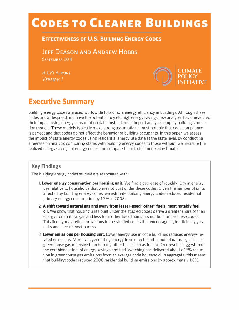
Codes to Cleaner BuildingsSummer 2011

Executive SummaryBuilding energy codes are used worldwide to promote energy efficiency in buildings. Although these codes are widespread and have the potential to yield high energy savings, few analyses have measured their impact using energy consumption data. Instead, most impact analyses employ building simula-tion models. These models typically make strong assumptions, most notably that code compliance is perfect and that codes do not affect the behavior of building occupants. In this paper, we assess the impact of state energy codes using residential energy use data at the state level. By conducting a regression analysis comparing states with building energy codes to those without, we measure the realized energy savings of energy codes and compare them to the modeled estimates.

Codes to Cleaner Buildings

Jeff Deason and Andrew HobbsSeptember 2011

Key FindingsThe building energy codes studied are associated with:

1. Lower energy consumption per housing unit. We find a decrease of roughly 10% in energy use relative to households that were not built under these codes. Given the number of units affected by building energy codes, we estimate building energy codes reduced residential primary energy consumption by 1.3% in 2008.

2. A shift toward natural gas and away from lesser-used “other” fuels, most notably fuel oil. We show that housing units built under the studied codes derive a greater share of their energy from natural gas and less from other fuels than units not built under these codes. This finding may reflect provisions in the studied codes that encourage high-efficiency gas units and electric heat pumps.

3. Lower emissions per housing unit. Lower energy use in code buildings reduces energy- re-lated emissions. Moreover, generating energy from direct combustion of natural gas is less greenhouse gas intensive than burning other fuels such as fuel oil. Our results suggest that the combined effect of energy savings and fuel-switching has delivered about a 16% reduc-tion in greenhouse gas emissions from an average code household. In aggregate, this means that building codes reduced 2008 residential building emissions by approximately 1.8%.

Effectiveness of U.S. Building Energy Codes

A CPI ReportVersion 1

iiA CPI Report

Codes to Cleaner BuildingsSeptember 2011

These findings are based on an econometric analysis that uses variation in the timing of state govern-ments’ implementation of building energy codes to isolate the impact of building codes from underly-ing time trends, state characteristics, construction rates, economic conditions, shifts in climate and prices. Our strategy ensures that the findings described above cannot be attributed to nationwide trends or individual state characteristics that might otherwise lead to inaccurate conclusions.

Our results to date cannot exclude the possibility that other state-level policy changes, such as appli-ance standards or utility demand-side management programs, had a role in these effects. If the intro-duction of other energy-saving programs by state is tightly coupled to code introduction, we may be attributing some savings to the energy codes that are in fact due to these other programs.

Our findings suggest that standard engineering estimates of energy savings are reasonable, at least for the studied codes; if anything, it appears that these estimates may be lower than actual savings. We confirm that building energy codes have reduced greenhouse gas emissions. Our findings also highlight the impact of codes on fuel choice, an effect we have not seen discussed elsewhere.

In future work, we will consider controlling for additional policies that may be relevant; assessing cost impacts of the codes; and comparing code savings across different states to identify effective imple-mentation and enforcement practices.

1A CPI Report


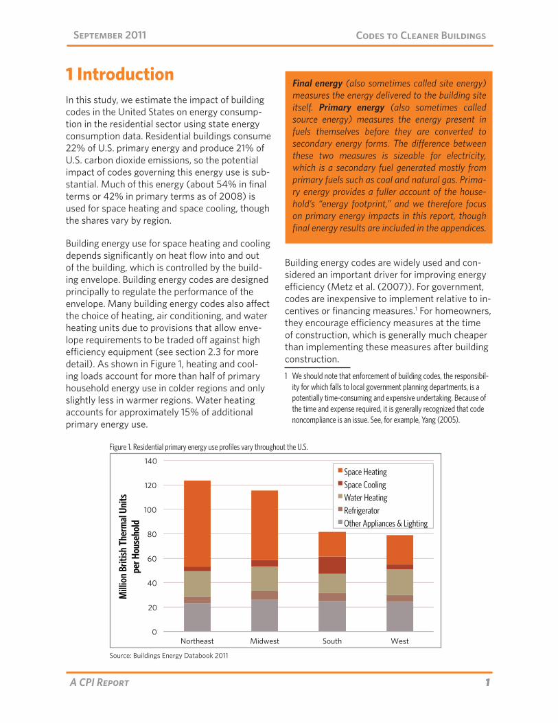
1 IntroductionIn this study, we estimate the impact of building codes in the United States on energy consump-tion in the residential sector using state energy consumption data. Residential buildings consume 22% of U.S. primary energy and produce 21% of U.S. carbon dioxide emissions, so the potential impact of codes governing this energy use is sub-stantial. Much of this energy (about 54% in final terms or 42% in primary terms as of 2008) is used for space heating and space cooling, though the shares vary by region.

Building energy use for space heating and cooling depends significantly on heat flow into and out of the building, which is controlled by the build-ing envelope. Building energy codes are designed principally to regulate the performance of the envelope. Many building energy codes also affect the choice of heating, air conditioning, and water heating units due to provisions that allow enve-lope requirements to be traded off against high efficiency equipment (see section 2.3 for more detail). As shown in Figure 1, heating and cool-ing loads account for more than half of primary household energy use in colder regions and only slightly less in warmer regions. Water heating accounts for approximately 15% of additional primary energy use.

Building energy codes are widely used and con-sidered an important driver for improving energy efficiency (Metz et al. (2007)). For government, codes are inexpensive to implement relative to in-centives or financing measures.1 For homeowners, they encourage efficiency measures at the time of construction, which is generally much cheaper than implementing these measures after building construction.

1 We should note that enforcement of building codes, the responsibil-ity for which falls to local government planning departments, is a potentially time-consuming and expensive undertaking. Because of the time and expense required, it is generally recognized that code noncompliance is an issue. See, for example, Yang (2005).

Final energy (also sometimes called site energy) measures the energy delivered to the building site itself. Primary energy (also sometimes called source energy) measures the energy present in fuels themselves before they are converted to secondary energy forms. The difference between these two measures is sizeable for electricity, which is a secondary fuel generated mostly from primary fuels such as coal and natural gas. Prima-ry energy provides a fuller account of the house-hold’s “energy footprint,” and we therefore focus on primary energy impacts in this report, though final energy results are included in the appendices.

Figure 1. Residential primary energy use profiles vary throughout the U.S.

Source: Buildings Energy Databook 2011

2A CPI Report


Section 2 of this paper describes building energy codes in the United States, including their history, development process, and an overview of their provisions. Section 3 reviews the literature on estimates of code impacts. Section 4 describes our methods and the data we used to estimate building energy code impacts. Section 5 presents our results to date. Section 6 discusses the policy implications of our results, and Section 7 identi-fies potential next steps for future research.

2 Residential Building Energy Codes in the United States

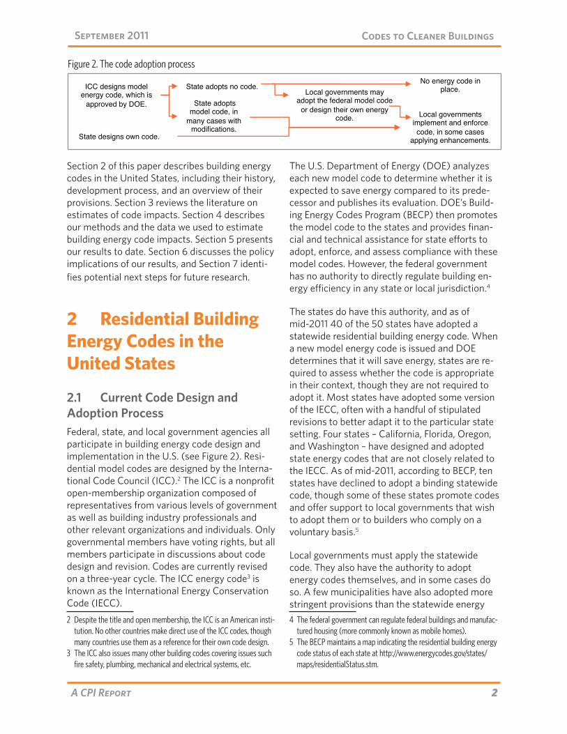
2.1 Current Code Design and Adoption ProcessFederal, state, and local government agencies all participate in building energy code design and implementation in the U.S. (see Figure 2). Resi-dential model codes are designed by the Interna-tional Code Council (ICC).2 The ICC is a nonprofit open-membership organization composed of representatives from various levels of government as well as building industry professionals and other relevant organizations and individuals. Only governmental members have voting rights, but all members participate in discussions about code design and revision. Codes are currently revised on a three-year cycle. The ICC energy code3 is known as the International Energy Conservation Code (IECC).

2 Despite the title and open membership, the ICC is an American insti-tution. No other countries make direct use of the ICC codes, though many countries use them as a reference for their own code design.

3 The ICC also issues many other building codes covering issues such fire safety, plumbing, mechanical and electrical systems, etc.

The U.S. Department of Energy (DOE) analyzes each new model code to determine whether it is expected to save energy compared to its prede-cessor and publishes its evaluation. DOE’s Build-ing Energy Codes Program (BECP) then promotes the model code to the states and provides finan-cial and technical assistance for state efforts to adopt, enforce, and assess compliance with these model codes. However, the federal government has no authority to directly regulate building en-ergy efficiency in any state or local jurisdiction.4

The states do have this authority, and as of mid-2011 40 of the 50 states have adopted a statewide residential building energy code. When a new model energy code is issued and DOE determines that it will save energy, states are re-quired to assess whether the code is appropriate in their context, though they are not required to adopt it. Most states have adopted some version of the IECC, often with a handful of stipulated revisions to better adapt it to the particular state setting. Four states – California, Florida, Oregon, and Washington – have designed and adopted state energy codes that are not closely related to the IECC. As of mid-2011, according to BECP, ten states have declined to adopt a binding statewide code, though some of these states promote codes and offer support to local governments that wish to adopt them or to builders who comply on a voluntary basis.5

Local governments must apply the statewide code. They also have the authority to adopt energy codes themselves, and in some cases do so. A few municipalities have also adopted more stringent provisions than the statewide energy 4 The federal government can regulate federal buildings and manufac-

tured housing (more commonly known as mobile homes).5 The BECP maintains a map indicating the residential building energy

code status of each state at http://www.energycodes.gov/states/maps/residentialStatus.stm.

Figure 2. The code adoption process

3A CPI Report


code, even where one is present.

2.2 History of Code Creation and AdoptionIn the early 1970s, some states began implement-ing building energy codes. The first code to see widespread adoption was the American Society of Heating, Refrigerating, and Air Conditioning Engi-neers (ASHRAE) Standard 90-75, issued in 1975 and backed by the Council of American Building Officials (CABO) in 1977 following a public hear-ing and revision process sponsored by the Energy Research and Development Administration (a predecessor to DOE). This code was updated in 1980 as Standard 90A-1980. It appears that most states had adopted a version of these codes by the time the first national model code was ad-opted in 1992 (Heldenbrand (2001)).

The Energy Policy Act of 1992 created the BECP and mandated DOE’s role in the development of model codes and in supporting state adop-tion. Since the program’s inception, the DOE has adopted codes designed by building associations comprised of government and private actors. The first residential model code was the 1992 Model Energy Code (MEC) issued by the CABO. Updates were issued in 1993 and 1995. CABO then merged

with several other buildings associations to form the ICC in 1998. The ICC issued the first IECC in 1998, with updates in 2000, 2003, 2006, and 2009. A new IECC will be adopted in 2012. The ICC has also issued occasional supplements to the code.

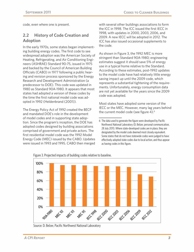
As shown in Figure 3, the 1992 MEC is more stringent than Standard 90A-1980; engineering estimates suggest it should save 5% of energy use in a typical home relative to the Standard. According to these estimates, post-1992 updates to the model code have had relatively little energy saving impact up until the 2009 code, which represents a substantial tightening of the require-ments. Unfortunately, energy consumption data are not yet available for the years since the 2009 code was adopted.

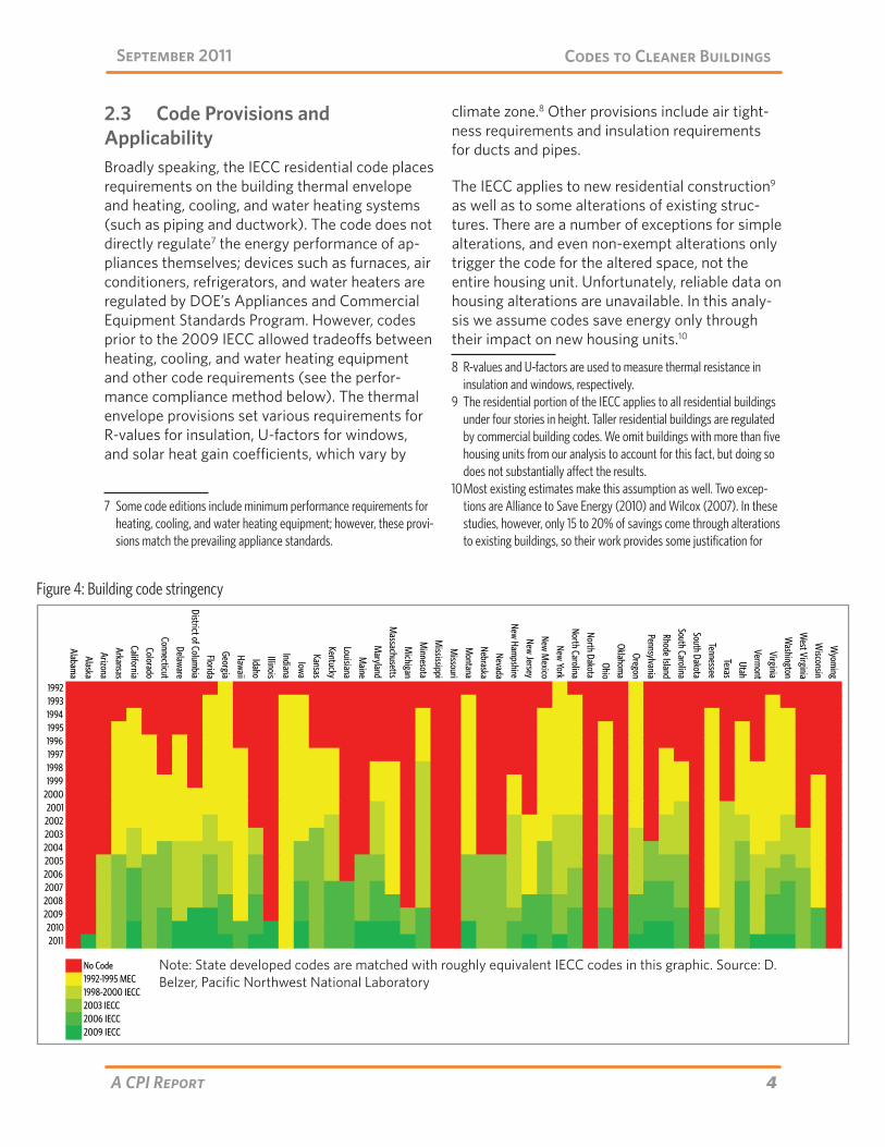
Most states have adopted some version of the IECC or the MEC. However, many lag years behind the current model code (see figure 4).6

6 The data used to generate the figure were developed by Pacific Northwest National Laboratory (D. Belzer, personal communication, 28 July 2011). Where state-developed codes are in place, they are designated by the model code deemed most closely equivalent. Some states that do not have statewide codes were judged to have effectively adopted state codes due to local action, and thus appear as having codes in this figure.

Figure 3. Projected impacts of building codes relative to baseline.

Source: D. Belzer, Pacific Northwest National Laboratory

4A CPI Report


2.3 Code Provisions and ApplicabilityBroadly speaking, the IECC residential code places requirements on the building thermal envelope and heating, cooling, and water heating systems (such as piping and ductwork). The code does not directly regulate7 the energy performance of ap-pliances themselves; devices such as furnaces, air conditioners, refrigerators, and water heaters are regulated by DOE’s Appliances and Commercial Equipment Standards Program. However, codes prior to the 2009 IECC allowed tradeoffs between heating, cooling, and water heating equipment and other code requirements (see the perfor-mance compliance method below). The thermal envelope provisions set various requirements for R-values for insulation, U-factors for windows, and solar heat gain coefficients, which vary by

7 Some code editions include minimum performance requirements for heating, cooling, and water heating equipment; however, these provi-sions match the prevailing appliance standards.

climate zone.8 Other provisions include air tight-ness requirements and insulation requirements for ducts and pipes.

The IECC applies to new residential construction9 as well as to some alterations of existing struc-tures. There are a number of exceptions for simple alterations, and even non-exempt alterations only trigger the code for the altered space, not the entire housing unit. Unfortunately, reliable data on housing alterations are unavailable. In this analy-sis we assume codes save energy only through their impact on new housing units.10

8 R-values and U-factors are used to measure thermal resistance in insulation and windows, respectively.

9 The residential portion of the IECC applies to all residential buildings under four stories in height. Taller residential buildings are regulated by commercial building codes. We omit buildings with more than five housing units from our analysis to account for this fact, but doing so does not substantially affect the results.

10 Most existing estimates make this assumption as well. Two excep-tions are Alliance to Save Energy (2010) and Wilcox (2007). In these studies, however, only 15 to 20% of savings come through alterations to existing buildings, so their work provides some justification for

Note: State developed codes are matched with roughly equivalent IECC codes in this graphic. Source: D. Belzer, Pacific Northwest National Laboratory

Figure 4: Building code stringency

5A CPI Report


To comply with the IECC, one may choose either the “prescriptive” or “performance” pathway. For the prescriptive pathway, one may either satisfy all provisions individually or choose a total build-ing approach that calculates the U-factor of the entire building thermal envelope while fulfilling other requirements individually. The performance pathway uses simulated building performance software to calculate the annual energy cost of the building as designed, ensuring that it is less than or equal to that of an equivalent building built in accordance with the individual provisions. DOE manages the development of the RESCheck software tool, which is approved by most states for total building U-factor calculations. While RE-SCheck is not a total building simulation, it does provide an approximate building-wide calculation that some states have approved for the perfor-mance path. State or local code officials are re-sponsible for approving other building simulation software for performance path determinations.

In model codes prior to 2009, installing a high-efficiency furnace meant the insulation require-ments for the remainder of the building were reduced. The 2009 IECC eliminates the ability to trade envelope requirements against unit per-formance. Many other codes, in U.S. states and overseas, continue to allow such tradeoffs.11

3 Existing WorkEven though building energy codes have existed in the U.S. for almost 40 years, evidence of their ef-fectiveness based on actual energy consumption data has only recently begun to emerge. Most estimates of code impact that we have found use building energy simulations to calculate the dif-ference between a typical unit’s energy consump-tion under the new code and under the previous code. They then multiply this amount by the total number of units constructed under the new code

focusing on new build impacts.11 Examples: In addition to previous versions of the IECC, which are still

in use in many states, the current version of California’s Title 24 code (which is not substantially based on the IECC) allows these tradeoffs in the performance path, as does the German energy code.

to estimate total code savings.12

Reasons to expect that end use energy savings caused by the code might differ from engineering estimates include:

• Code compliance. Engineering calculations im-plicitly assume that code compliance is per-fect. In fact, many studies (see Yang (2005) for a summary) have shown that compliance is far from perfect. Moreover, even where there is apparent compliance, mis-installation or improper maintenance can reduce the energy-saving impact of code measures.

• Non-additional code provisions. These calcula-tions assume that the energy-saving mea-sures required by the new code would not have been undertaken without the code. This may not always be the case; for example, technological improvements might lead to en-ergy savings even if the code did not require them.

• Rebound effect. An improved building envelope makes it cheaper to heat and cool, as less conditioned air is lost to the environment. As a result, building occupants may increase their use of space conditioning to some extent, offsetting some of the energy savings the envelope generates. Building energy simu-lations do not factor in behavioral responses of this kind.

• Spillover effect. Building codes may affect building practices regionally and lead to improvements in practice outside of their jurisdictions. If this is the case, our model will underestimate the effect of energy codes, as it will be comparing them to a baseline that is also experiencing some energy savings from the code. These spillover benefits will not be captured by our estimates.

Our econometric analysis embeds these factors. Our estimate yields the net impact of the codes; however, it is silent on the relative impacts of these factors.

12Analyses using variants of this calculation include Alliance to Save Energy (2010), Wilcox (2007), and Pacific Northwest National Laboratory (2009).

6A CPI Report


The earliest econometric study we are aware of that tests the impact of building energy codes with energy use data is Jaffe and Stavins (1995). The authors use several variables, including build-ing codes, to explain the level of installed thermal insulation in new home construction in the U.S. They find that the studied codes do not have a statistically significant effect on insulation lev-els. Their explanation is that most codes in their study (all of which predated the 1992 MEC) were likely non-additional in the sense that standard insulation practice already met or exceeded them. Arimura et al. (2009) study the impact of utility demand-side management on state electricity consumption over a similar time frame to our study and include building codes as a controlling variable. Their best estimate of code impacts is a very small electricity savings.

On the other hand, three recent studies focus on codes and show statistically significant impacts. Jacobsen and Kotchen (2010) study the impact of a single change to the Florida state code on electricity and natural gas consumption using household-level billing data. They show that per-residence electricity and natural gas consumption decreased by approximately 4% and 6% respec-tively after the implementation of the code, and that these changes are not explained by pre-ex-isting trends. Costa and Kahn (2010) use house-hold-level data in a California county to show that building codes have been associated with reduced residential electricity demand. They do not esti-mate effects on natural gas consumption. Aroon-ruengsawat et al. (2009) is the closest cousin to our study. The authors use variation in code adoption by state over time to identify the effect of codes on residential electricity consumption in the U.S. They find that building energy codes are associated with a 2 to 5% reduction in per capita residential electricity consumption. They also show the level of effort states exert to implement and enforce code compliance, as measured by the American Council for an Energy Efficient Economy (ACEEE)’s State Energy Efficiency Scorecard, is useful in explaining code impacts: states with a better score show greater electricity savings. They do not estimate code effects on the consumption of natural gas or other fuels.

4 Study Methods and DataThis study estimates the effect of building energy codes on residential energy consumption and greenhouse gas emissions at the state level. We examine code impacts on electricity, natural gas, and other fuels individually, as well as impacts on total final and primary energy consumption and greenhouse gas emissions. In order to isolate the impact of the codes, we control for other impor-tant factors affecting building energy consump-tion, such as energy prices, economic conditions, weather, climate, and residential construction rates. Our model also accounts for factors that do not vary across states, such as federal policy or nationwide trends. Our data cover the 48 con-tinental U.S. states and the years 1986 through 2008. See Appendix A for details on the data.

To put our strategy to work, we need to know when each state adopted each version of the code. Code adoption data are based on a data-base compiled by staff involved in the Depart-ment of Energy’s Building Energy Codes Program at the Pacific Northwest Laboratory.13 The data indicate when each state adopted each fed-eral model code, beginning with the 1992 MEC. Where states develop their own codes, the PNNL data match the state code with the most similar national model code at the time.

Combining data on new construction and code status, we measure the fraction of occupied units in a given state built under an energy code at least as stringent as the 1992 MEC. This is the primary variable of interest for our analysis. If building energy codes save energy, states with a larger percentage of housing stock built under a code should consume less energy per housing unit, holding all else equal. We regress this variable on various measures of residential energy use in each state in each year. Our model controls for the other variables discussed above as well as for

13 Data supplied by D. Belzer, PNNL. In addition to work by staff at PNNL, the code adoption dates are also based upon newsletters pub-lished by the Building Codes Assistance Project (BCAP). See website http://bcap-energy.org/.

7A CPI Report


nationwide time trends and state-specific factors that might distort our result. Refer to Appendix B for a more detailed discussion of our modeling methodology.

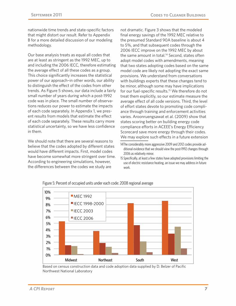
Our base analysis treats as equal all codes that are at least as stringent as the 1992 MEC, up to and including the 2006 IECC, therefore estimating the average effect of all these codes as a group. This choice significantly increases the statistical power of our approach–in other words, our ability to distinguish the effect of the codes from other trends. As Figure 5 shows, our data include a fairly small number of years during which a post-1992 code was in place. The small number of observa-tions reduces our power to estimate the impacts of each code separately. In Appendix 1, we pres-ent results from models that estimate the effect of each code separately. These results carry more statistical uncertainty, so we have less confidence in them.

We should note that there are several reasons to believe that the codes adopted by different states would have different impacts. First, model codes have become somewhat more stringent over time. According to engineering simulations, however, the differences between the codes we study are

not dramatic. Figure 3 shows that the modeled final energy savings of the 1992 MEC relative to the presumed Standard 90A baseline is about 4 to 5%, and that subsequent codes through the 2006 IECC improve on the 1992 MEC by about the same amount in total.14 Second, states often adopt model codes with amendments, meaning that two states adopting codes based on the same model code are likely not adopting the exact same provisions. We understand from conversations with buildings experts that these changes tend to be minor, although some may have implications for our fuel-specific results.15 We therefore do not treat them explicitly, so our estimate measure the average effect of all code versions. Third, the level of effort states devote to promoting code compli-ance through training and enforcement activities varies. Aroonruengsawat et al. (2009) show that states scoring better on building energy code compliance efforts in ACEEE’s Energy Efficiency Scorecard save more energy through their codes. We may explore such effects in a future extension

14The considerably more aggressive 2009 and 2012 codes provide ad-ditional evidence that we should view the post-1992 changes through 2006 as relatively minor.

15 Specifically, at least a few states have adopted provisions limiting the use of electric resistance heating, an issue we may address in future work.

Figure 5: Percent of occupied units under each code: 2008 regional average

Based on census construction data and code adoption data supplied by D. Belzer of Pacific Northwest National Laboratory

8A CPI Report


of this analysis. In the end we are confident that none of these issues invalidates our choice to pool all the codes for this study.

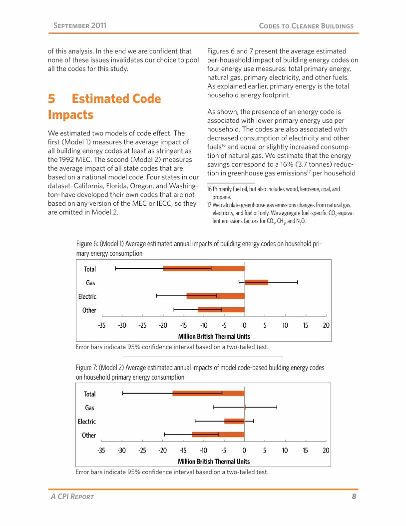
5 Estimated Code ImpactsWe estimated two models of code effect. The first (Model 1) measures the average impact of all building energy codes at least as stringent as the 1992 MEC. The second (Model 2) measures the average impact of all state codes that are based on a national model code. Four states in our dataset–California, Florida, Oregon, and Washing-ton–have developed their own codes that are not based on any version of the MEC or IECC, so they are omitted in Model 2.

Figures 6 and 7 present the average estimated per-household impact of building energy codes on four energy use measures: total primary energy, natural gas, primary electricity, and other fuels. As explained earlier, primary energy is the total household energy footprint.

As shown, the presence of an energy code is associated with lower primary energy use per household. The codes are also associated with decreased consumption of electricity and other fuels16 and equal or slightly increased consump-tion of natural gas. We estimate that the energy savings correspond to a 16% (3.7 tonnes) reduc-tion in greenhouse gas emissions17 per household

16 Primarily fuel oil, but also includes wood, kerosene, coal, and propane.

17 We calculate greenhouse gas emissions changes from natural gas, electricity, and fuel oil only. We aggregate fuel-specific CO2-equiva-lent emissions factors for CO2, CH4, and N2O.

Figure 6: (Model 1) Average estimated annual impacts of building energy codes on household pri-mary energy consumption

Error bars indicate 95% confidence interval based on a two-tailed test.

Figure 7: (Model 2) Average estimated annual impacts of model code-based building energy codes on household primary energy consumption

Error bars indicate 95% confidence interval based on a two-tailed test.

9A CPI Report


per year in Model 1 and an 11% (2.6 tonnes) reduction per household per year in Model 2.

Our overall results are similar for the two mod-els. However, Model 1 shows a large, statistically significant decrease in electricity use and a small increase in natural gas use, while Model 2 shows a smaller decrease in electricity use and essen-tially no change in gas use. We must therefore be cautious in ascribing effects on these two fuels to the model codes; it appears that the four state-developed codes may have rather different impacts. We discuss this issue further in Section 5.2 below.

5.1 Impacts on Primary Energy UseWe find that the energy codes studied are saving energy in residential buildings. Model 1 suggests 11% primary energy savings, while Model 2 sug-gests 10%. Both results are statistically signifi-cant. Aggregating the Model 1 savings estimate over all code-built housing units in 2008, the final year of our data, indicates that the studied codes saved 28 trillion BTUs of energy in that year. This represents 1.3% of U.S. primary residential energy use in 2008.

Our best estimates of the effect of codes on pri-mary energy consumption are higher than simula-tions suggest. Combining data on the number of units constructed under each code with simulated estimates from Pacific Northwest National Lab, the average home built under a code during the period studied would be expected to reduce its energy consumption by 5%. While our estimates are higher, 5% is contained in the confidence interval of both estimates.18

There are several factors that could help explain why our estimates of energy savings per housing unit are higher than the engineering estimates:

• Our current model does not control for other policy (such as appliance standards and utility DSM programs) that would be expected to

18 5% savings is within the 95% confidence interval in both model. The 5% estimate is also within the 90% confidence interval in Model 2, though it is just outside the 90% confidence interval in Model 1.

reduce household energy use. If states19 tend to adopt these other measures at the same time as they adopt building energy codes,20 our current model would attribute some of the impacts of these programs to codes.

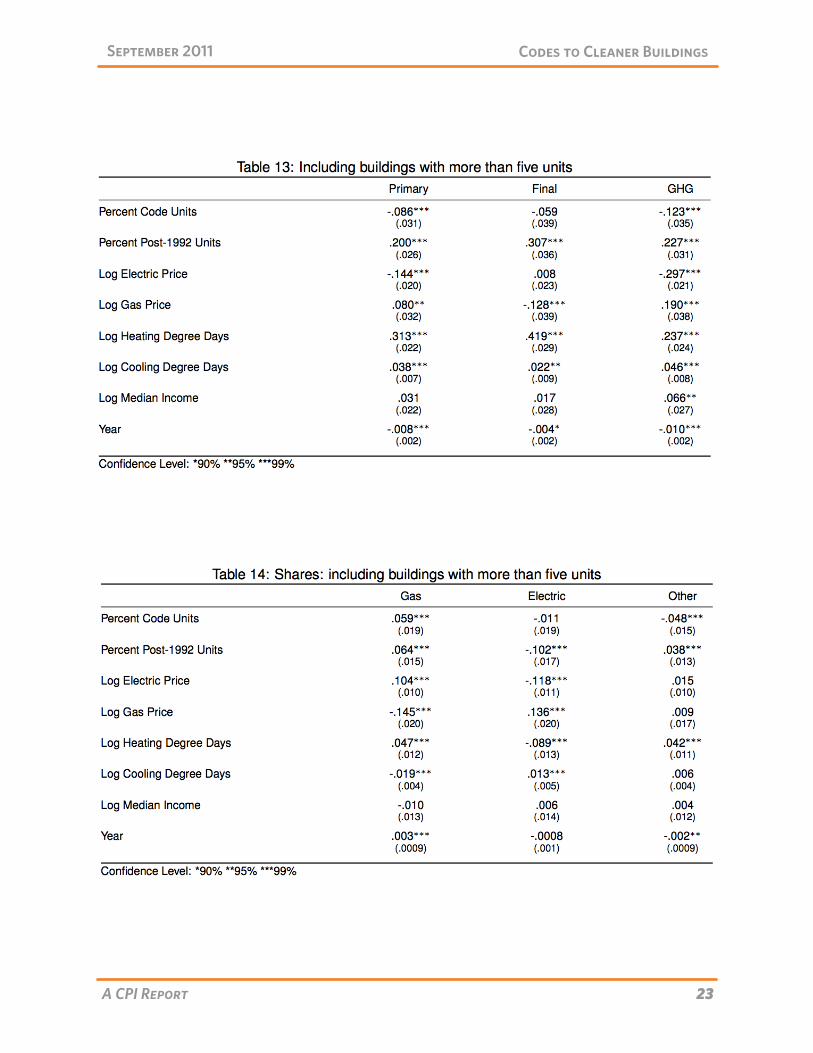
• Due to data limitations, it is likely that we excluded some housing units from our count of code-built units. In order to eliminate large buildings covered by commercial codes, we dropped all units in buildings with more than five units. This means we are attributing over-all energy savings from the code to a smaller number of units, increasing the per-unit effect size. When we run the same analysis with all of these units included, our per-unit primary energy savings estimate in Model 1 drops but only to 9% (see Appendix A and Table 13 for more). This value provides a robust lower bound estimate, as this model certainly overestimates the number of units affected by the code. The number of code units assumed should have no effect on our calculation of total code savings, however.

• Relatedly, we do not account for the sav-ings codes may achieve through retrofits of existing buildings. As discussed in Section 2.3 above, some existing analyses suggest that 15 to 20% of code impacts may come through retrofit. If true, our estimates of primary en-ergy impacts per new housing unit are about 2% too high. Again, our total energy savings estimates should still be accurate.

• In constructing the engineering estimate, we use Standard 90A-1980 to estimate baseline energy use. If instead some of these states had no code, or codes inferior to Standard 90A-1980, prior to adopting a post-1992 MEC code, then the baseline energy efficiency in our data is worse than the engineering esti-mate baseline, meaning our results would not be comparable to the engineering estimates. This factor does not affect the accuracy of our

19 Federal regulatory activity would not be an issue here, as our fixed effects econometric model controls for changes that affect all states at the same time; see Appendix B for discussion of the model.

20 Arimura et al. (2009) show that building code adoption and utility DSM expenditures are slightly correlated in their dataset, which is similar to ours.

10A CPI Report


estimate, but rather the validity of the com-parison to the engineering estimate.

On the other hand, one factor suggests that our results may miss some energy savings created by the codes. When codes advance building practice in jurisdictions that adopt them, there is reason to expect that these advances may “spill over” into other states as builders adapt and learn. Our models do not account for such effects, and thereby undercount savings in two ways. First, savings in states without codes are not credited to the codes by our model. Second, non-code states in our models form the baseline off of which code savings are estimated. If the energy use of these states embeds some savings, this baseline is more efficient than a true no-code baseline, and it therefore appears that codes are saving less than they really are.

Given the uncertainty in our model as well as the factors discussed in the previous paragraphs, we view our results as consistent with the engineer-ing estimates, suggesting that, if anything, the engineering estimates are too low.

5.2 Fuel-Specific ImpactsUse of “other” fuels –primarily fuel oil– has fallen in both models; these results are statistically sig-nificant. Model 1 shows a statistically significant decrease in electricity use of approximately the same percentage as the overall decrease in energy use. Model 2 shows a smaller effect on electricity that is not statistically significant. Model 1 sug-gests that natural gas use has risen, though the finding is not statistically significant; Model 2 shows no effect on natural gas use.

In interpreting these results, we note that each is a composite of two effects: a general decrease in energy use and, potentially, a shift in fuel choice. This is particularly notable for electricity, which comprises a large share of residential primary energy in the U.S. When we predict the share of energy use for each fuel with our regression model, we learn that the electricity share is un-changed in Model 1 and actually goes up in Model 2. Gas shares go up and “other” shares down in both models.

As noted in section 2.3, the model codes in this study allow energy-saving tradeoffs between heating and water heating units and the build-ing envelope where the performance pathway is elected. These provisions specifically encour-aged natural gas heating and water heating and electric heat pumps, while discouraging electric resistance heat. The increases in natural gas use that we observe are consistent with this provision, while the decrease in use of other fuels suggests substitution away from them and towards natural gas or heat pumps.

As for electricity, the net impact of the code provi-sions on fuel choice is ambiguous, as they en-courage heat pumps while discouraging electric resistance heating. Model 1 (all building energy codes) shows a stronger reduction in electricity use than Model 2 (codes based on national model only). This suggests the four state-developed codes might include stronger provisions to dis-courage electricity use. In fact, the three West Coast states have code provisions that discourage electric resistance heat. Heating is a relatively small contributor to building energy consumption in the fourth state (Florida), so we would expect little energy impact from any heating-related fuel-switching that the codes did motivate.

5.3 Impacts on Greenhouse Gas EmissionsBoth models show substantial and statistically significant reductions in greenhouse gas emis-sions associated with codes. Model 1 estimates a 16% reduction in emissions per household, while Model 2 estimates 11%. The fact that Model 1 estimates greater greenhouse gas reductions can be traced to the fuel-specific impacts. Model 1 (and by implication the four states excluded from Model 2) shows more natural gas use and less electricity use in code households. Burning natural gas in the home is considerably less emissions-intensive than consuming electricity from the current U.S. generation mix.

Taking the per-household reduction estimate noted under Model 1 above and multiplying it by the 14 million households built under one of the

11A CPI Report


studied codes in 2008, we estimate that emis-sions were 52 million tonnes CO2-equivalent lower in 2008 than they would have been had in the absence of energy codes. This is about 1.8% of U.S. greenhouse gas emissions from residen-tial buildings in 2008 (U.S. Department of En-ergy (2010)). As building energy codes become stricter and the proportion of residential buildings built under modern codes rises, these savings can be expected to increase significantly.

6 Policy ImplicationsWe highlight four points for policy that follow from our study.

First, building energy codes clearly appear to be successful in saving energy in residential build-ings. Notwithstanding potential complications created by noncompliance, non-additional codes, and rebound effects, our models show savings with a high level of certainty. The average per household energy savings (measured in either final or primary terms) delivered by energy codes in the period from 1992-2008 are on the order of ten percent relative to prior practice.

Second, building energy codes have been effective in reducing greenhouse gas emissions from build-ings. Our model estimates that houses built under energy code regimes were associated with 16% lower greenhouse gas emissions, yielding a 1.8% overall reduction in residential building emissions in 2008.

Third, our results suggest that the studied codes delivered savings that are similar to those es-timated by engineering models. Our estimates based on ex post energy use data are somewhat higher, though several factors noted in section 5.1 may explain this discrepancy. Moreover, the un-certainty in our estimates of code impacts means they are not inconsistent with the engineering estimates. Coupled with other recent findings (Aroonruengsawat et al. (2009) and Jacobsen and Kotchen (2010)), our results suggest that none of the above-noted complications is signifi-cant enough to warrant a systematic downward

adjustment to modeled savings.

Fourth, code provisions affecting fuel choice–through the use of the performance pathway for compliance or through state-specific provisions–appear to have had an impact. The compliance pathway provisions are probably efficient policy in the short run, but may be less so in the long run. A unit that takes advantage of these tradeoffs may install a less efficient envelope than would otherwise be allowed. Envelopes are a more permanent building feature than heating, cooling, or water heating units. Therefore, these buildings will likely be less efficient than they otherwise would be once these original units have been replaced. Moreover, as the U.S. electric supply is decarbonized, natural gas units will deliver fewer emissions savings. Policymakers will need to bal-ance these short run and longer-run impacts. We note that the 2009 IECC no longer allows these tradeoffs, although some states (e.g., California) and nations (e.g., Germany) do.

7 Potential Next Steps/Future WorkWe have identified the following avenues for po-tential future research, and welcome feedback:

• Consider cost impacts of the codes. We can calculate the operational savings from re-duced energy bills achieved by codes using our data. We could then compare them to estimates of the additional up-front cost imposed by the codes to get a sense of the payback period and dollar savings achieved by the codes for households. We could also consider such impacts for the states and the country as a whole. Such findings could be useful as indicators of potential savings for states that have not yet adopted these codes.

• Incorporate variables into our model that con-trol for other state-level policies such as ap-pliance standards and utility DSM programs. The DSM variable would reflect various en-ergy efficiency measures, both for new build and retrofit, that should help explain residen-

12A CPI Report


tial energy consumption. Appliance standards would also affect both new build and retrofit, though there is relatively little state-specific appliance regulation. Including these variables would allow us to better isolate the impact of codes from other coincident policy. We might also want to include a variable recognizing those states that have included significant disincentives to electric resistance heating in their code amendments.

• Attempt to identify which states are achieving greater energy savings and emissions reduc-tions through these codes through their im-plementation and enforcement efforts. A first step in this analysis would be to incorporate a variable for level of state effort in the model, as Aroonruengsawat et al. (2009) do with the ACEEE Scorecard. If this variable has explana-tory power (as it does in Aroonruengsawat et al. (2009)), we will have reason to believe that implementation and enforcement have significant differential impacts and are worth investigating. We should note that imple-mentation and enforcement occur largely at the local levels, which means that state-level analysis could miss important differences.

• Explore the possibility of regional spillovers. It is possible that improved building practices in states with building energy codes also have some impact on neighboring states. If neigh-boring states benefit from building codes, code effects may be greater than our current estimates suggest.

13A CPI Report


ReferencesAlliance to Save Energy (2010). Potential na-

tionwide savings from adoption of the 2012 IECC. Technical report.

Arimura, T., Newell, R. G., and Palmer, K. (2009). Cost-effectiveness of electricity energy efficiency programs. SSRN eLibrary.

Aroonruengsawat, A., Auffhammer, M., and Sanstad, A. (2009). The impact of state level building codes on residential electricity consumption. Working Paper.

Belzer, D. (2011). Personal communication. Technical report, Pacific Northwest National Laboratory.

Costa, D. L. and Kahn, M. E. (2010). Why has California’s residential electricity con-sumption been so flat since the 1980s?: A microeconometric approach. Working Paper 15978, National Bureau of Economic Research.

Energy Information Administration (2010). State energy data system. Technical report. Hel-denbrand, J. L. (2001). Design and Evalua-tion Criteria for Energy Conservation in New Buildings. National Institute of Standards and Technology, Gaithersburg, MD.

Jacobsen, G. D. and Kotchen, M. J. (2010). Are building codes effective at saving energy? evidence from residential billing data in Florida. Working Paper 16194, National Bureau of Economic Research.

Jaffe, A. B. and Stavins, R. N. (1995). Dynamic incentives of environmental regulations: The effects of alternative policy instru-ments on technology diffusion. Journal of Environmental Economics and Management, 29(3):43–63.

Metz, B., Davidson, O. R., Bosch, P. R., Dave, R., and Meyer, L. (2007). Residential and Commercial Buildings. Cambridge University Press, Cambridge, United Kingdom and New York, NY, USA.

National Climatic Data Center (2011). Heating and cooling degree day data. Technical report.

Pacific Northwest National Laboratory (2009). Impacts of the 2009 IECC for residential buildings at state level. Technical report.

U. S. Census Bureau (2011a). Income. Technical report.

U. S. Census Bureau (2011b). New residential construction. Technical report.

U.S. Department of Energy (2010). Buildings Energy Databook.

Wilcox, B. (2007). 2008 update to the California energy efficiency standards for residential and nonresidential buildings. Technical report, Architectural Energy Corporation.

Yang, B. (2005). Residential energy code evaluations: Review and future directions. Technical report, Building Codes Assistance Project.

14A CPI Report


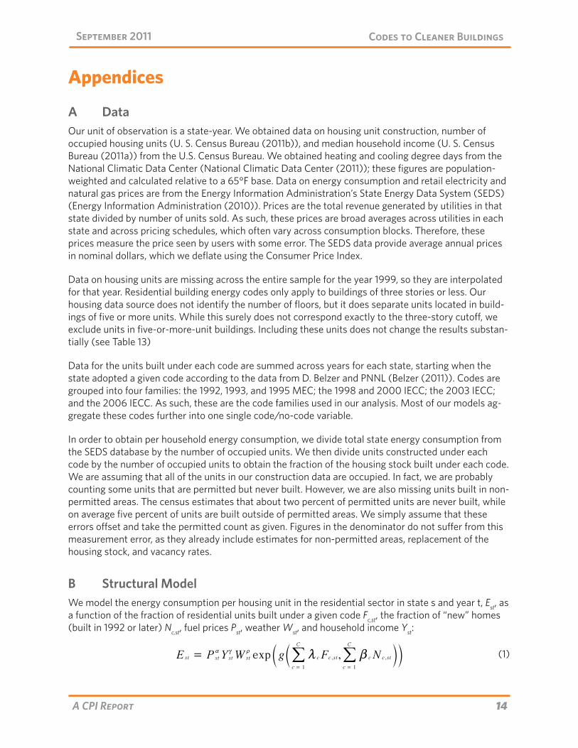
Appendices

A DataOur unit of observation is a state-year. We obtained data on housing unit construction, number of occupied housing units (U. S. Census Bureau (2011b)), and median household income (U. S. Census Bureau (2011a)) from the U.S. Census Bureau. We obtained heating and cooling degree days from the National Climatic Data Center (National Climatic Data Center (2011)); these figures are population-weighted and calculated relative to a 65°F base. Data on energy consumption and retail electricity and natural gas prices are from the Energy Information Administration’s State Energy Data System (SEDS) (Energy Information Administration (2010)). Prices are the total revenue generated by utilities in that state divided by number of units sold. As such, these prices are broad averages across utilities in each state and across pricing schedules, which often vary across consumption blocks. Therefore, these prices measure the price seen by users with some error. The SEDS data provide average annual prices in nominal dollars, which we deflate using the Consumer Price Index.

Data on housing units are missing across the entire sample for the year 1999, so they are interpolated for that year. Residential building energy codes only apply to buildings of three stories or less. Our housing data source does not identify the number of floors, but it does separate units located in build-ings of five or more units. While this surely does not correspond exactly to the three-story cutoff, we exclude units in five-or-more-unit buildings. Including these units does not change the results substan-tially (see Table 13)

Data for the units built under each code are summed across years for each state, starting when the state adopted a given code according to the data from D. Belzer and PNNL (Belzer (2011)). Codes are grouped into four families: the 1992, 1993, and 1995 MEC; the 1998 and 2000 IECC; the 2003 IECC; and the 2006 IECC. As such, these are the code families used in our analysis. Most of our models ag-gregate these codes further into one single code/no-code variable.

In order to obtain per household energy consumption, we divide total state energy consumption from the SEDS database by the number of occupied units. We then divide units constructed under each code by the number of occupied units to obtain the fraction of the housing stock built under each code. We are assuming that all of the units in our construction data are occupied. In fact, we are probably counting some units that are permitted but never built. However, we are also missing units built in non-permitted areas. The census estimates that about two percent of permitted units are never built, while on average five percent of units are built outside of permitted areas. We simply assume that these errors offset and take the permitted count as given. Figures in the denominator do not suffer from this measurement error, as they already include estimates for non-permitted areas, replacement of the housing stock, and vacancy rates.

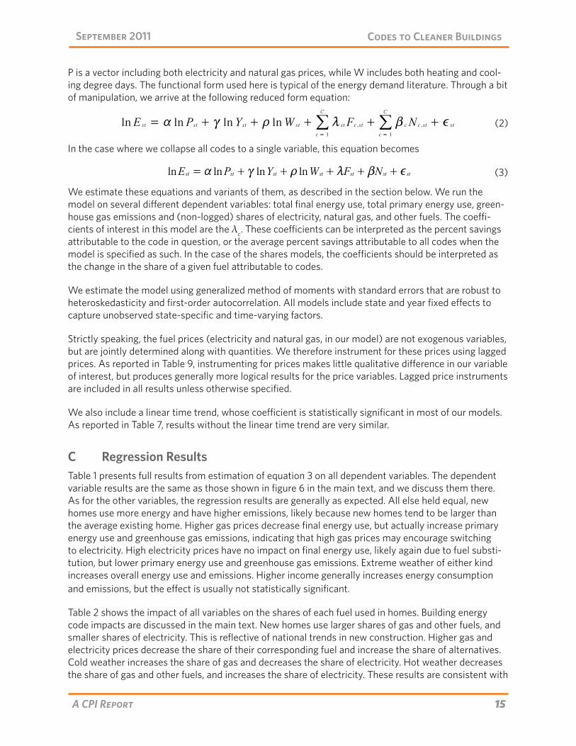
B Structural ModelWe model the energy consumption per housing unit in the residential sector in state s and year t, Est, as a function of the fraction of residential units built under a given code Fc,st, the fraction of “new” homes (built in 1992 or later) Nc,st, fuel prices Pst, weather Wst, and household income Yst:

(1)Est = PstaYstcWst

texp g m c Fc ,st, b c N c ,st

c = 1

C

/c = 1

C

/c mc m

15A CPI Report


P is a vector including both electricity and natural gas prices, while W includes both heating and cool-ing degree days. The functional form used here is typical of the energy demand literature. Through a bit of manipulation, we arrive at the following reduced form equation:

In the case where we collapse all codes to a single variable, this equation becomes

We estimate these equations and variants of them, as described in the section below. We run the model on several different dependent variables: total final energy use, total primary energy use, green-house gas emissions and (non-logged) shares of electricity, natural gas, and other fuels. The coeffi-cients of interest in this model are the λc. These coefficients can be interpreted as the percent savings attributable to the code in question, or the average percent savings attributable to all codes when the model is specified as such. In the case of the shares models, the coefficients should be interpreted as the change in the share of a given fuel attributable to codes.

We estimate the model using generalized method of moments with standard errors that are robust to heteroskedasticity and first-order autocorrelation. All models include state and year fixed effects to capture unobserved state-specific and time-varying factors.

Strictly speaking, the fuel prices (electricity and natural gas, in our model) are not exogenous variables, but are jointly determined along with quantities. We therefore instrument for these prices using lagged prices. As reported in Table 9, instrumenting for prices makes little qualitative difference in our variable of interest, but produces generally more logical results for the price variables. Lagged price instruments are included in all results unless otherwise specified.

We also include a linear time trend, whose coefficient is statistically significant in most of our models. As reported in Table 7, results without the linear time trend are very similar.

C Regression ResultsTable 1 presents full results from estimation of equation 3 on all dependent variables. The dependent variable results are the same as those shown in figure 6 in the main text, and we discuss them there. As for the other variables, the regression results are generally as expected. All else held equal, new homes use more energy and have higher emissions, likely because new homes tend to be larger than the average existing home. Higher gas prices decrease final energy use, but actually increase primary energy use and greenhouse gas emissions, indicating that high gas prices may encourage switching to electricity. High electricity prices have no impact on final energy use, likely again due to fuel substi-tution, but lower primary energy use and greenhouse gas emissions. Extreme weather of either kind increases overall energy use and emissions. Higher income generally increases energy consumption and emissions, but the effect is usually not statistically significant.

Table 2 shows the impact of all variables on the shares of each fuel used in homes. Building energy code impacts are discussed in the main text. New homes use larger shares of gas and other fuels, and smaller shares of electricity. This is reflective of national trends in new construction. Higher gas and electricity prices decrease the share of their corresponding fuel and increase the share of alternatives. Cold weather increases the share of gas and decreases the share of electricity. Hot weather decreases the share of gas and other fuels, and increases the share of electricity. These results are consistent with

ln Est = a ln Pst + c ln Yst + t lnWst + m st Fc ,st + b c N c ,st + e stc = 1

C

/c = 1

C

/ (2)

lnEst = a lnPst+ c lnYst+ t lnWst+ mFst+ bNst+ est (3)

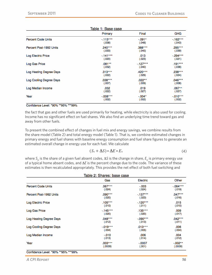
16A CPI Report


the fact that gas and other fuels are used primarily for heating, while electricity is also used for cooling. Income has no significant effect on fuel shares. We also find an underlying time trend toward gas and away from other fuels.

To present the combined effect of changes in fuel mix and energy savings, we combine results from the share model (Table 2) and total energy model (Table 1). That is, we combine estimated changes in primary energy and fuel shares with baseline energy consumption and fuel share figures to generate an estimated overall change in energy use for each fuel. We calculate

where S0 is the share of a given fuel absent codes, ∆S is the change in share, E0 is primary energy use of a typical home absent codes, and ∆E is the percent change due to the code. The variance of these estimates is then recalculated appropriately. This provides the net effect of both fuel switching and

S0 +DS^ h )DE ) E0 (4)

17A CPI Report


energy savings. Intuitively, this captures the fact that although the share of a given fuel may remain unchanged, reductions in the household total may yield a net reduction.

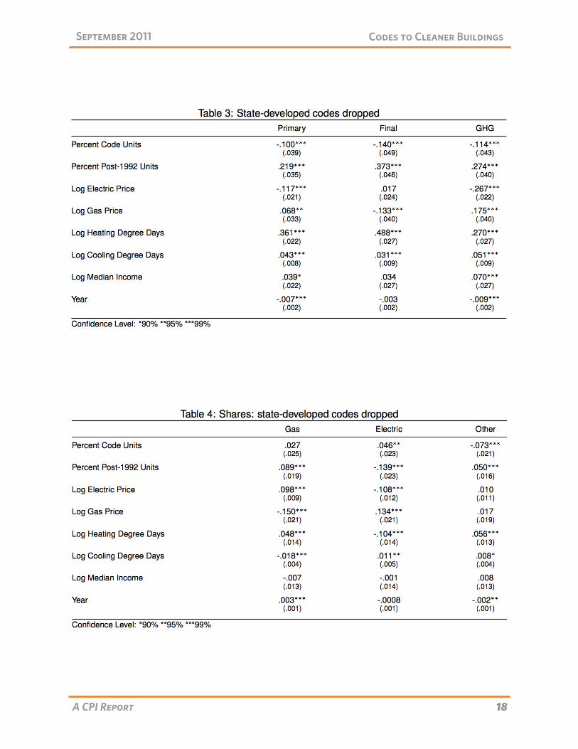
Table 3 shows the impact of dropping states with state-developed codes. Again, the codes variable is discussed in the main text. Results for all other variables are very similar to the previous model.

In Table 5 we present results of models including separate variables for the number of units built under each of the four code groups provided by Belzer and PNNL. Results for the 1992-1995 MEC codes are broadly consistent with the results in the aggregate model, though some findings are less statistically significant. Results for the 1998-2003 codes are generally consistent with the aggregate model, but are almost never statistically significant; the results for other fuels begin to behave erratically. The 2006 results are strange, but they are based on a very small number of state-years, and these codes are not present for a sufficient portion of the panel for the results to be reliable. Given these results, we have more confidence in our models that aggregate codes.

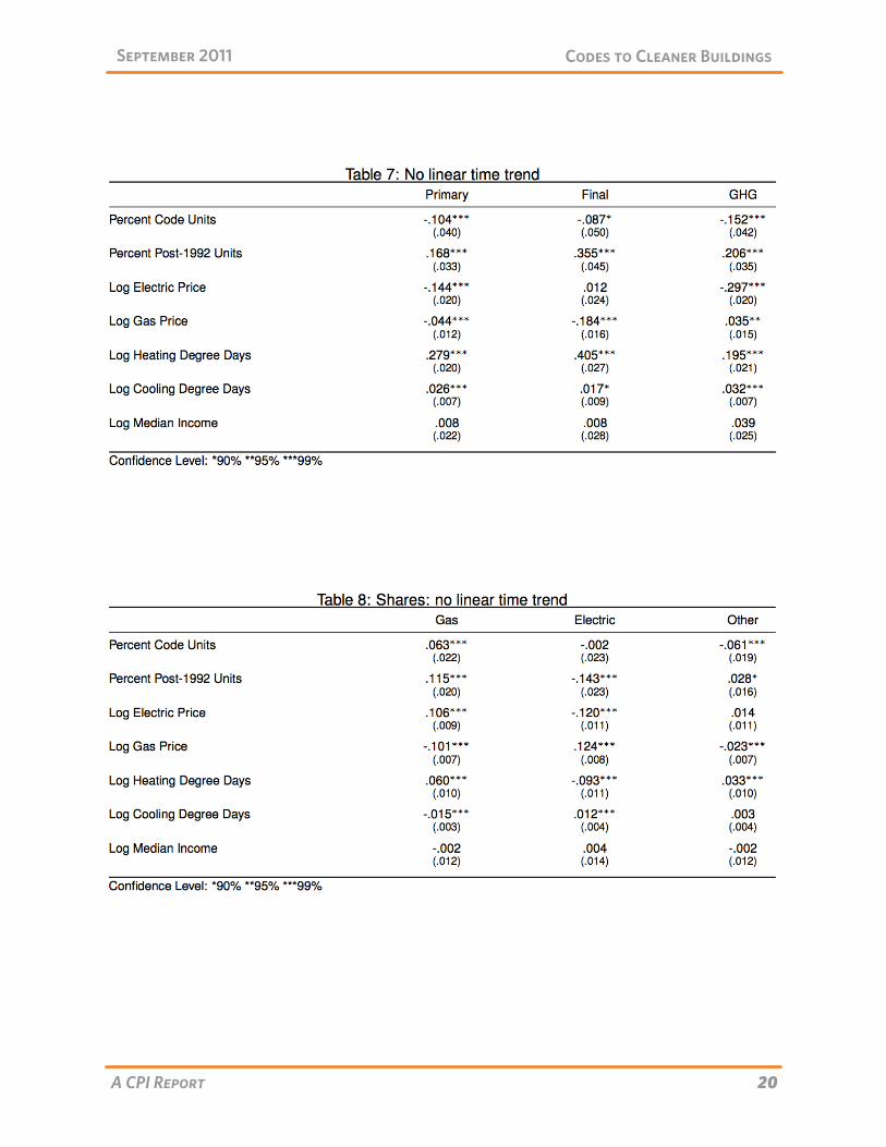
Table 7 shows the regression results without the linear time trend, though year dummies are still in place. No substantive changes occur.

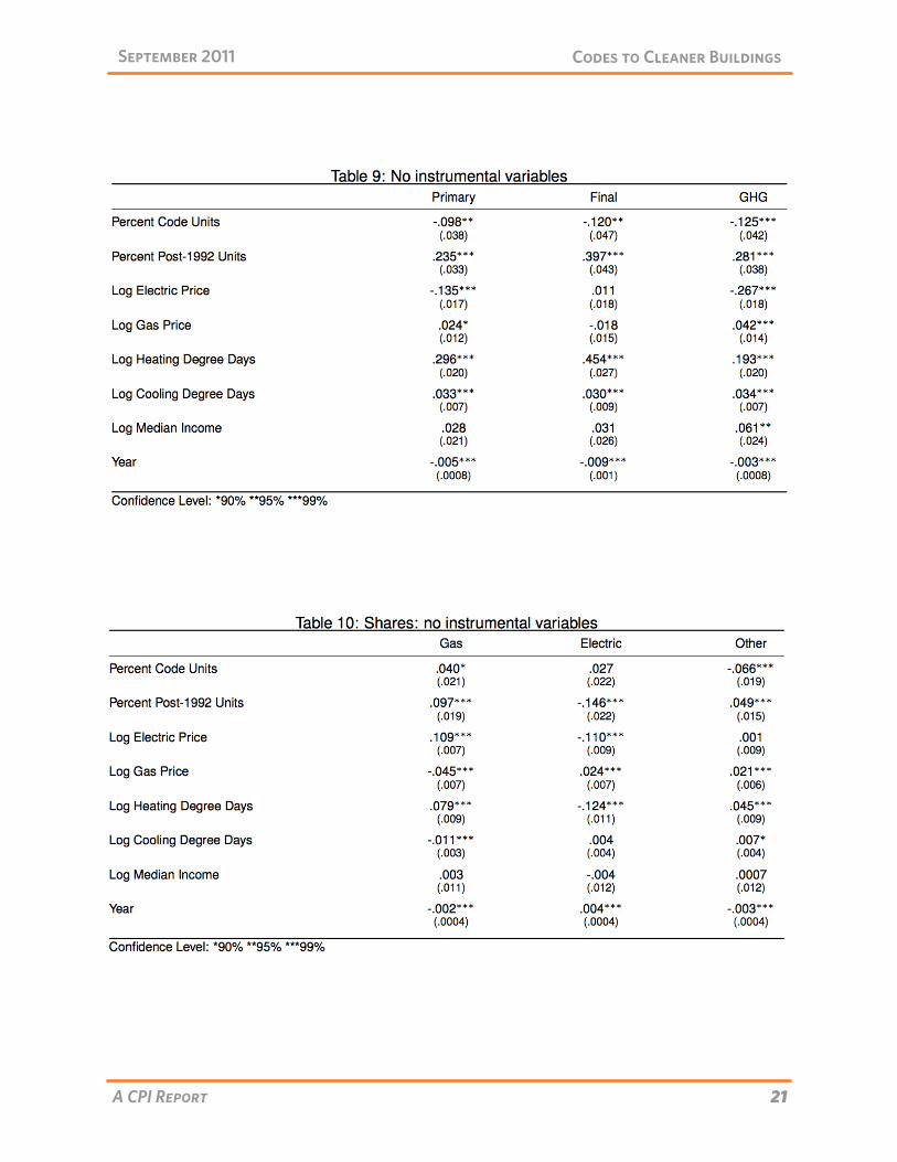
Table 9 shows the model without instrumenting for price. No substantial changes occur in the variable of interest.

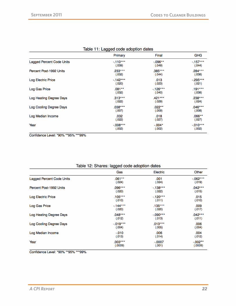
One potential issue for our analysis is that codes are adopted and made effective at various times dur-ing the calendar year. PNNL attempted to track the effective date of the code, rather than the adopted date, in their data; they also set the date to the subsequent calendar year if the code became effec-tive during the last four months of a year. However, even with these data practices, there is reason to explore lagging the codes. Code compliance is generally checked at the design stage when permits are submitted. Therefore, some buildings finished shortly after a new code has been implemented may have already been approved, and compliance may not be checked after the code change. We report results from lagging all code adoption dates by one year in Table 11 below. Results are very similar to the base model, indicating that the PNNL dates track actual code implementation well.

As noted in the Data section above, we exclude housing units in buildings of five or more units from our dataset, but this does not exactly correspond to the set of buildings the residential code covers (those that are three stories or less). In table 13 we provide results including these units. Results are similar, though the final energy savings lose significance and all code impact estimates move towards zero.

18A CPI Report


19A CPI Report


20A CPI Report


21A CPI Report


22A CPI Report


23A CPI Report


Documents

Summer 2011 Codes to Cleaner Buildings - CPIclimatepolicyinitiative.org/wp-content/uploads/2011/12/Codes-to... · CPI Working Paper i Summer 2011 Codes to Cleaner Buildings Executive