Sudden Stops, Financial Crises, and Leverage - sas.upenn.eduegme/pp/CompletePaperRevforDistribution.pdf · VOL. 100 NO. 5 mENDOzA: SuDDEN STOPS, FINANCIAL CRISES, AND LEVERAGE 1943

1941

American Economic Review 100 (December 2010): 1941–1966http://www.aeaweb.org/articles.php?doi=10.1257/aer.100.5.1941

“ … debt happens as a result of actions occurring over time. Therefore, any debt involves a plot line: how you got into debt, what you did, said and thought while you were there, and then—depending on whether the ending is to be happy or sad—how you got out of debt, or else how you got further and further into it until you became overwhelmed by it, and sank from view.” (Margaret Atwood, Wall Street Journal, 09/20/2008, p. W1)

A key lesson of the Great Depression and the ongoing global economic crisis is that financial crashes are followed by deep recessions that differ markedly from typical business cycles. The Sudden Stops that hit many emerging economies in the aftermath of their financial crashes since the 1980s illustrate the same fact, and hence they provide a unique laboratory to study the link-ages between financial collapse and macroeconomic crisis. This paper proposes an equilibrium business cycle model with an endogenous collateral constraint and shows that its quantitative predictions are in line with the stylized facts of Sudden Stops.

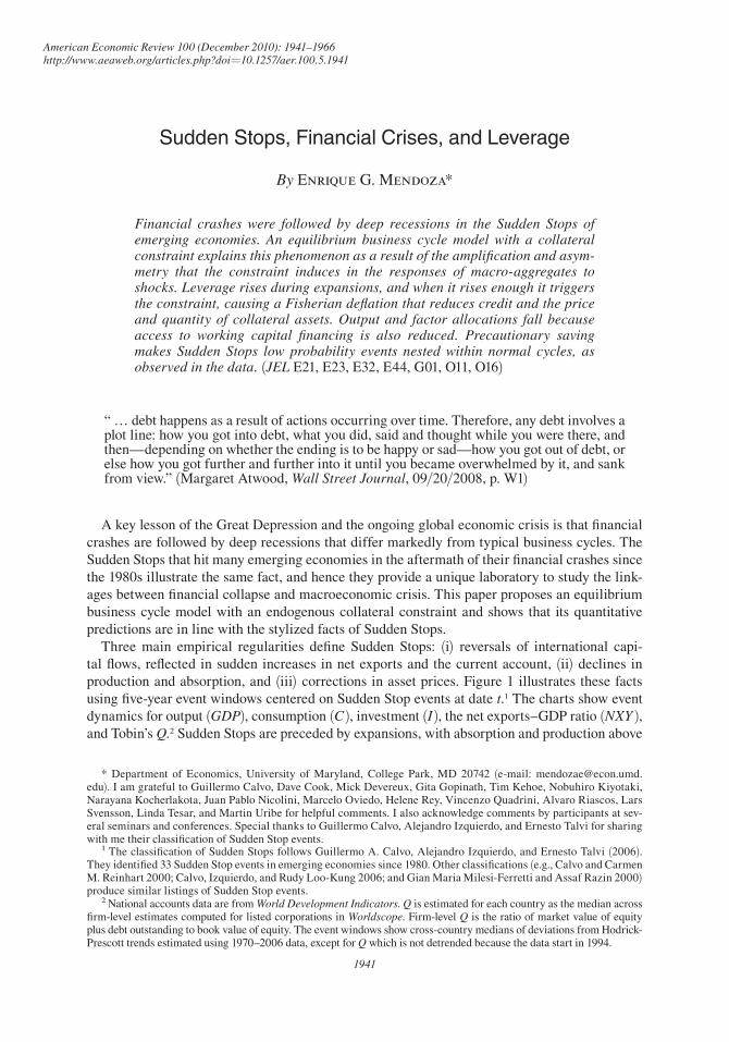
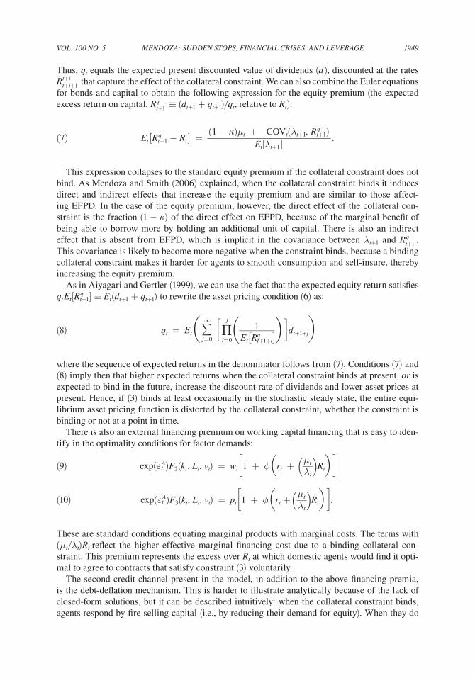
Three main empirical regularities define Sudden Stops: (i) reversals of international capi-tal flows, reflected in sudden increases in net exports and the current account, (ii) declines in production and absorption, and (iii) corrections in asset prices. Figure 1 illustrates these facts using five-year event windows centered on Sudden Stop events at date t.1 The charts show event dynamics for output (GDP), consumption (C ), investment (I ), the net exports–GDP ratio (NXY ), and Tobin’s Q.2 Sudden Stops are preceded by expansions, with absorption and production above

1 The classification of Sudden Stops follows Guillermo A. Calvo, Alejandro Izquierdo, and Ernesto Talvi (2006). They identified 33 Sudden Stop events in emerging economies since 1980. Other classifications (e.g., Calvo and Carmen M. Reinhart 2000; Calvo, Izquierdo, and Rudy Loo-Kung 2006; and Gian Maria Milesi-Ferretti and Assaf Razin 2000) produce similar listings of Sudden Stop events.

2 National accounts data are from World Development Indicators. Q is estimated for each country as the median across firm-level estimates computed for listed corporations in Worldscope. Firm-level Q is the ratio of market value of equity plus debt outstanding to book value of equity. The event windows show cross-country medians of deviations from Hodrick-Prescott trends estimated using 1970–2006 data, except for Q which is not detrended because the data start in 1994.

Sudden Stops, Financial Crises, and Leverage

By Enrique G. Mendoza*

Financial crashes were followed by deep recessions in the Sudden Stops of emerging economies. An equilibrium business cycle model with a collateral constraint explains this phenomenon as a result of the amplification and asym-metry that the constraint induces in the responses of macro-aggregates to shocks. Leverage rises during expansions, and when it rises enough it triggers the constraint, causing a Fisherian deflation that reduces credit and the price and quantity of collateral assets. Output and factor allocations fall because access to working capital financing is also reduced. Precautionary saving makes Sudden Stops low probability events nested within normal cycles, as observed in the data. (JEL E21, E23, E32, E44, G01, O11, O16)

* Department of Economics, University of Maryland, College Park, MD 20742 (e-mail: [email protected]). I am grateful to Guillermo Calvo, Dave Cook, Mick Devereux, Gita Gopinath, Tim Kehoe, Nobuhiro Kiyotaki, Narayana Kocherlakota, Juan Pablo Nicolini, Marcelo Oviedo, Helene Rey, Vincenzo Quadrini, Alvaro Riascos, Lars Svensson, Linda Tesar, and Martin Uribe for helpful comments. I also acknowledge comments by participants at sev-eral seminars and conferences. Special thanks to Guillermo Calvo, Alejandro Izquierdo, and Ernesto Talvi for sharing with me their classification of Sudden Stop events.

DECEmBER 20101942 THE AmERICAN ECONOmIC REVIEW

trend, the trade balance below trend, and high asset prices. The median Sudden Stop displays a reversal in the cyclical component of NXY of about 3 percentage points at date t. GDP and C are about 4 percentage points below trend, and I collapses almost 20 percentage points below trend. A weak recovery follows, but GDP, C, and I remain below trend two years later.3 Q reaches a

3 The quicker recovery shown in Calvo, Izquierdo, and Talvi (2006) follows from two differences in the event analysis. First, they compute cross-country averages of country-specific cumulative growth. We use medians instead of averages because of substantial cross-country dispersion in cyclical components, and deviations from trend instead of cumulative growth to remove low-frequency dynamics. Second, Calvo, Izquierdo, and Talvi focus mainly on Sudden Stops with large output collapses. Here we include all Sudden Stop events.

t − 2 t − 1 t t + 1 t + 2

Gross domestic product Private consumption

Investment

0.800

0.850

0.900

0.950

1.000

1.050

Tobin Q

Net exports–GDP ratio

t − 2 t − 1 t t + 1 t + 2

t − 2 t − 1 t t + 1 t + 2 t − 2 t − 1 t t + 1 t + 2

t − 2 t − 1 t t + 1 t + 2

6.00

4.00

2.00

0.00

−2.00

−4.00

−6.00

6.00

4.00

2.00

0.00

−2.00

−4.00

−6.00

Per

cent

Per

cent

3.00

2.00

1.00

0.00

−1.00

−2.00

−3.00

Per

cent

20.00

15.00

10.00

5.00

0.00

−5.00

−10.00

−15.00

−20.00

Per

cent

Figure 1. Macroeconomic Dynamics around Sudden Stop Events in Emerging Economies (cross-country medians of deviations from HP trends)

Notes: The classification of Sudden Stop events in the emerging markets data is taken from Calvo, Izquierdo, and Talvi (2006). They define systemic sudden stop events as episodes with mild and large output collapses that coincide with large spikes in the EMBI spread and large reversals in capital flows. Tobin’s Q is the ratio of market value of equity and debt outstanding over book value of equiy, and it is shown in levels instead of deviation from HP trend.

VOL. 100 NO. 5 1943mENDOzA: SuDDEN STOPS, FINANCIAL CRISES, AND LEVERAGE

trough at date t 13 percentage points below the pre–Sudden Stop peak, and it recovers about two-thirds of its value by t + 2.

The sharp economic fluctuations experienced during Sudden Stops also display three key properties that models aiming to explain this phenomenon should account for: first, Sudden Stops are infrequent events nested within typical business cycles. They are rare events by defini-tion, because a key criterion to identify them is that a country’s international capital flows are significantly below their mean (see Calvo, Izquierdo, and Talvi 2006). Second, they represent business cycle asymmetries (i.e., we do not observe symmetric episodes of sudden large drops in trade surpluses accompanied by surges in output and absorption). Third, a drop in the Solow residual, rather than declines in capital and labor, accounts for a large fraction of a Sudden Stops’ initial output drop, and this is due in part to factors that bias Solow residuals as a measure of “true” total factor productivity (TFP), such as changes in imported inputs, capacity utilization, and labor hoarding (see Mendoza 2006, and Felipe Meza and Erwan Quintin 2007). The model proposed here is consistent with these three features of actual Sudden Stops.

Explaining Sudden Stops is a challenge for a large class of dynamic stochastic general equilib-rium (DSGE) models, including frictionless real business cycle models and models with nominal rigidities. This is because these models typically assume credit markets that are an efficient vehicle for consumption smoothing and investment financing. For example, in response to a large output drop, households smooth the effect on consumption by borrowing from abroad, while in Sudden Stops we observe the opposite (the external accounts rise sharply precisely when con-sumption and output collapse). In contrast, the literature on Sudden Stops views credit frictions as the central feature of the transmission mechanism that drives Sudden Stops (e.g., Leonardo Auernheimer and Roberto Garcia-Saltos 2000; Ricardo J. Caballero and Arvind Krishnamurty 2001; Calvo 1998; Gita Gopinath 2004; Woon Gyu Choi and David Cook 2004; Cook and Michael B. Devereux 2006a, 2006b; Philippe Martin and Helen Rey 2006; Mark Gertler, Simon Gilchrist, and Fabio M. Natalucci 2007; and Fabio Braggion, Lawrence J. Christiano, and Jorge Roldos 2009). The model proposed in this paper follows on a similar path, but it focuses on the amplification and asymmetry of macroeconomic fluctuations that result from Irving Fisher’s (1933) classic debt-deflation transmission mechanism.

The model introduces a Fisherian endogenous collateral constraint into a DSGE model driven by standard exogenous shocks to TFP, the foreign interest rate, and the price of imported intermediate goods. The collateral constraint limits total debt, including both intertemporal debt and atemporal working capital loans, not to exceed a fraction of the market value of the physical capital that serves as collateral. Thus, the constraint imposes a ceiling on the leverage ratio. The emphasis is on studying the quantitative significance of this credit friction, along the lines of the literature on the macroeconomic implications of credit constraints (as in Nobuhiro Kiyotaki and John Moore 1997; Ben S. Bernanke and Gertler 1989; Bernanke, Gertler, and Gilchrist 1998; S. Rao Aiyagari and Gertler 1999; Narayana Kocherlakota 2000; Thomas F. Cooley, Ramon Miramon, and Vincenzo Quadrini 2004; and Urban Jermann and Vincenzo Quadrini 2009).

The results of the quantitative analysis show that the model explains the key stylized facts of Sudden Stops. Comparing economies with and without the collateral constraint, both exhibit largely the same long-run business cycle moments, but the former displays significant amplifica-tion and asymmetry in the responses of macro-aggregates to one–standard-deviation shocks. Amplification is reflected in larger mean responses in states in which the constraint binds. Asymmetry is shown in that the responses to shocks of identical magnitudes are about the same in the two economies if the collateral constraint does not bind.

Sudden Stop events in the model are very similar to the actual events illustrated in Figure 1. In particular, the model matches well the behavior of GDP, C, I, and NXY. Moreover, the Solow


residual overestimates the true state of TFP by about 30 percent. The model also replicates the dynamics of Q qualitatively, but quantitatively it underestimates the collapse of asset prices.

The collateral constraint adds three important elements to the business cycle transmission mechanism that are crucial for the model’s favorable quantitative results:

(i) The constraint is occasionally binding, because it binds only when the leverage ratio is sufficiently high. When this happens, typical realizations of the exogenous shocks produce Sudden Stops. If the constraint does not bind, the shocks yield similar macroeconomic responses as in a typical DSGE model with working capital. As a result, the economy dis-plays “normal” business cycle patterns when the collateral constraint does not bind.

(ii) The loss of credit market access is endogenous.4 In particular, the high leverage ratios at which the collateral constraint binds are reached after sequences of realizations of the exogenous shocks lead the endogenous business cycle dynamics to states with sufficiently high leverage. Since net exports are countercyclical, these high-leverage states are pre-ceded by economic expansions, as observed in emerging economies. However, Sudden Stops have a low long-run probability of occurring, because agents accumulate precau-tionary savings to reduce the likelihood of large consumption drops. Hence, Sudden Stops are rare events nested within typical business cycles.

(iii) Sudden Stops are driven by two sets of “credit channel” effects. The first are endog-enous financing premia that affect intertemporal debt, working capital loans, and equity, because the effective cost of borrowing rises when the collateral constraint binds. The second is the debt-deflation mechanism: when the constraint binds, agents are forced to liquidate capital. This fire sale of assets reduces the price of capital and tightens fur-ther the constraint, setting off a spiraling collapse in the price and quantity of collateral assets. Consumption, investment, and the trade deficit suffer contemporaneous reversals as a result, and future capital, output, and factor allocations fall in response to the initial investment decline. In addition, the reduced access to working capital induces contempo-raneous drops in production and factor demands.

It is important to note that standard DSGE models cannot produce Sudden Stops even if work-ing capital and/or imported inputs are added. Agents in these models still have access to a fric-tionless credit market, and hence negative shocks to TFP and/or imported input prices induce typical RBC-like responses. Large shocks could trigger large output collapses driven in part by cuts in imported inputs, but this would still fail to explain the current account reversal and the collapse in consumption (since households would borrow from abroad to smooth consumption). Adding large shocks to the world interest rate or access to external financing can alter these results, but such a theory of Sudden Stops hinges on unexplained “large and unexpected” shocks. Large because by definition they need to induce recessions larger than normal non–Sudden Stop recessions, and unexpected because otherwise agents would self-insure against their real effects. In contrast, this paper shows that the Fisherian collateral constraint provides an explanation for endogenous Sudden Stops that does not hinge on large, unexpected shocks.

The collateral constraint used in this paper is similar to the margin constraint used by Mendoza and Katherine A. Smith (2006) in their open economy extension of the Aiyagari-Gertler (1999) set-up. The model studied here differs in that it is a full-blown equilibrium business cycle model

4 In contrast, the initial reversal of the external accounts is generally modeled as a large, unexpected shock to credit or the interest rate in most of the Sudden Stops literature (e.g., Calvo 1998; Braggion, Christiano, and Roldos 2009).


with endogenous capital accumulation and dividend payments that vary in response to the collat-eral constraint, and the constraint limits access to both intertemporal debt and working capital. In contrast, Mendoza and Smith study a set-up in which production and dividends are unaffected by the credit constraint, abstract from modeling capital accumulation, and consider a credit con-straint that limits only intertemporal debt.

This paper is also closely related to two strands of the literature that study the quantitative implications of financial constraints for emerging markets business cycles. One is the strand that studies the effects of working capital financing on long-run business cycle comovements (see P. Andres Neumeyer and Fabrizio Perri 2005; Martin Uribe and Vivian Z. Yue 2006; and P. Marcelo Oviedo 2004). The model of this paper differs in one key respect: working capital loans require collateral, so that when the collateral constraint binds, the cutoff in working capital loans contributes to the amplification and asymmetry observed in the Sudden Stop responses of output and factor demands. Moreover, the model is parameterized so that only a small fraction of factor costs is paid in advance. As a result, working capital without the collateral constraint makes little difference for business cycle dynamics (relative to a frictionless economy).

The second strand is the one that introduced the Bernanke-Gertler financial accelerator into DSGE models with nominal rigidities. Notably, Gertler, Gilchrist, and Natalucci (2007) cali-brated a model of this class to Korean data and studied its ability to account for the 1997–1998 Korean crash as a response to a large shock to the world real interest rate. In addition, Gertler, Gilchrist, and Natalucci introduced a mechanism to drive the output collapse together with a decline in the Solow residual by modeling variable capital utilization. This paper introduces a different financial accelerator mechanism, based on an occasionally binding collateral con-straint, and uses imported intermediate goods to produce a decline in the Solow residual.5 The qualitative interpretation of the feedback between asset prices and debt is similar to the one in Gertler, Gilchrist, and Natalucci, but the strong nonlinear features of the debt-deflation mecha-nism yield endogenous Sudden Stops that do not require large, unexpected shocks and coexist with regular business cycles. On the other hand, since solving the model requires nonlinear global solution methods for models with incomplete markets, the model is less flexible than the framework of Gertler, Gilchrist, and Natalucci for studying the role of the financial accelerator in large-scale DSGE models.

The paper is organized as follows: Section I describes the model and its competitive equilib-rium. Sections II and III conduct the quantitative analysis. Section IV concludes.

I. A Model of Sudden Stops and Business Cycles with Collateral Constraints

A. Optimization Problem of the Representative Firm-Household

Consider a small open economy (SOE) inhabited by an infinitely lived, self-employed repre-sentative firm-household.6 Preferences are defined over stochastic sequences of consumption ct

and labor supply Lt, for t =0, … , ∞, using Larry G. Epstein’s (1983) Stationary Cardinal Utility (SCU) function. SCU features an endogenous rate of time preference that enables the model to support a unique, invariant limiting distribution of foreign assets under incomplete markets.7

5 A previous version of this paper used both imported inputs and variable utilization (see Mendoza 2006). The latter was harder to calibrate, and its contribution was quantitatively smaller.

6 Mendoza (2006) presents a different decentralization in which firms and households are separate agents facing separate collateral constraints. The set-up used here yields very similar predictions and is simpler to describe and solve (I am grateful to an anonymous referee for suggesting this approach).

7 Epstein showed that SCU requires weaker preference axioms than the standard utility function with exogenous discounting. He also proved that a preference order consistent with those axioms can be expressed as a time-recursive


Since the SOE faces noninsurable income shocks and its interest rate is exogenous, precautionary saving would lead foreign assets to diverge to infinity with the standard assumption of a constant rate of time preference equal to the interest rate.8

The preference specification is:

(1) E0c ∑t=0

∞

exp e− ∑τ=0

t−1

ρ(cτ−N(Lτ))f u(ct−N(L t))d .

In this expression, u(·) is a standard twice–continuously differentiable and concave period utility function and ρ(·) is an increasing, concave and twice–continuously differentiable time prefer-ence function. Following Jeremy Greenwood, Zvi Hercowitz, and Gregory W. Huffman (1988), utility is defined in terms of the excess of consumption relative to the disutility of labor, with the latter given by the twice–continuously differentiable, convex function N(·). This assumption eliminates the wealth effect on labor supply by making the marginal rate of substitution between consumption and labor independent of consumption.

Gross output in this economy is defined by a constant-returns-to-scale technology, exp(εt A

)F (k t , Lt , vt ), that requires capital, kt , labor and imported inputs, vt , to produce a tradable good sold at a world-determined price (normalized to unity without loss of generality). TFP is subject to a random shock εt A

with exponential support. Net investment, zt = kt+1 − kt, incurs unitary costs determined by a linearly homogeneous function of zt and kt, Ψ(z t/kt ).9 Working capital loans pay for a fraction ϕ of the cost of imported inputs and labor in advance of sales. These loans are obtained from foreign lenders at the beginning of each period and repaid at the end. Lenders charge the world gross real interest rate Rt =Rexp(εt R

) on these loans, where εt R

is an interest rate shock around a mean value R. Imported inputs are purchased at an exogenous relative price in terms of the world’s numeraire pt =p exp(εt P

), where p is the mean price and εt P

is a shock to the world price of imported inputs (i.e., a terms-of-trade shock from the perspective of the SOE). The shocks εt A

, εt R , and εt P

follow a first-order Markov process to be specified later.The representative agent chooses sequences of consumption, labor, investment, and holdings

of real, one-period international bonds, bt +1, so as to maximize SCU subject to the following period budget constraint:

(2) ct + it = exp(ε t A )F(k t , Lt , vt ) − pt vt − ϕ(Rt − 1)(wt Lt + pt vt ) − q t

b bt +1 + bt

where it =δkt + (kt +1 − kt) c1 + Ψ a kt +1 − kt _______kt

b d

utility function if and only if it takes the form of the SCU. Hence, ad hoc formulations of endogenous discounting in which the discount factor is independent of individual consumption deliver stationary net foreign assets, but they are inconsistent with the preference axioms.

8 Another model-based approach to obtain a stationary distribution of assets is to set a constant rate of time prefer-ence higher than the interest rate (see Aiyagari 1994). There are also three ad hoc approaches proposed by Stephanie Schmitt-Grohé and Uribe (2003) for use when solving models by perturbation methods (i.e., a cost of holding assets, a debt-elastic interest rate function, or a rate of time preference that depends on aggregate consumption). A model-based approach is more accurate for studying nonlinear effects and the effects of precautionary savings, but it requires global solution methods.

9 Specifying the capital adjustment cost in terms of net investment, instead of gross investment, yields a more trac-table recursive formulation of the economy’s optimization problem while preserving Fumio Hayashi’s (1982) results regarding the conditions that equate marginal and average Tobin Q.


is gross investment. The agent also faces the following collateral constraint:

(3) q t b bt +1 − ϕRt(wt L t + pt vt ) ≥ −κq t kt +1 .

In the constraints (2) and (3), wt is the wage rate, q t b is the price of bonds, and qt is the price

of domestic capital. The price of bonds is exogenous and satisfies q t b =1/Rt , while wt and qt are

endogenous prices that the agent takes as given and satisfy standard market optimality condi-tions (i.e., qt = ∂it (

_k t +1,

_k t)/∂ (

_k t +1)and wt =∂N(

__L t )/∂

__L t , where variables with bars are “mar-

ket averages” taken as given by the representative agent but equal to the representative agent’s choices at equilibrium).

The left-hand side of (2) is total domestic demand. The right-hand side is total sup-ply: GDP (gross output minus the cost intermediate goods, exp(ε t

A )F(k t , L t , vt) − pt vt) net of

interest payments abroad on working capital loans (ϕ(Rt − 1)(wt Lt + pt vt)) and of changes in foreign bond holdings inclusive of interest (q t

b bt +1 − bt ). Rearranging (2), we obtain the

accounting equality for the “real” and financial sides of the economy’s balance of trade: exp(ε t

A )F(k t , L t , vt) − ptvt − ct − it =ϕ(Rt − 1)(wt Lt + pt vt) + q t

b bt +1 − bt .

The collateral constraint (3) implies that total debt, including both debt in one-period bonds and working capital loans, cannot exceed a fraction κ of the “marked-to-market” value of capital (i.e., κ imposes a ceiling on the leverage ratio). Interest and principal on working capital loans enter in (3) because these are within-period loans, and thus lenders consider that collateral must cover both components.

The collateral constraint is not derived from an optimal credit contract but imposed directly as in other macro models with endogenous credit constraints (e.g., Kiyotaki and Moore 1997; Aiyagari and Gertler 1999; and Kocherlakota 2000). A constraint like (3) could result, for exam-ple, from an environment in which limited enforcement prevents lenders from collecting more than a fraction κ of the value of a defaulting debtor’s assets. As we explain below, when (3) binds, the model produces endogenous premia over the world interest rate at which borrowers would agree to contracts which satisfy (3).

It is also important to note that a variety of actual contractual arrangements can produce debt-deflation dynamics. The collateral constraint (3) resembles most directly a contract with a mar-gin clause. This clause requires borrowers to surrender the control of collateral assets when the contract is entered and gives creditors the right to sell them when their market value falls below the contract value. Other widely used arrangements that can trigger debt-deflation dynamics include value-at-risk strategies of portfolio management used by investment banks, and mark-to-market capital requirements imposed by regulators. For example, if an aggregate shock hits capi-tal markets, value-at-risk estimates increase and lead investment banks to reduce their exposure, but since the shock is aggregate, the resulting sale of assets increases price volatility and leads value-at-risk models to require further portfolio adjustments. Mechanisms like these played a central role in the Russian/LTCM crisis of 1998 and the US credit crisis of 2007–2008.

The assumption that the collateral constraint (3) applies to a representative agent acting com-petitively is not innocuous. On one hand, the competitive equilibrium is inefficient because the representative agent (ignoring the implications of its actions on the prices that enter in (3)) main-tains a suboptimally low level of precautionary savings, and hence is exposed to Sudden Stops with higher probability than a social planner that internalizes the constraint.10 On the other hand, in a model with heterogeneous agents facing (3) at the individual level, instead of a representative

10 Note, however, that Javier Bianchi (2009) compared the two equilibria in a Sudden Stops model similar to Mendoza (2002) and found that debt levels differ by small margins, and the NBER working paper version of Mendoza


agent, the fraction of agents hitting the collateral constraint would move over the business cycle because the Fisherian deflation process would have a cross-sectional dimension.

B. Competitive Equilibrium and Credit Channels

A competitive equilibrium for this model is defined by stochastic sequences of allocations [ct , Lt, kt +1, bt +1, vt, it ] 0

∞and prices [qt, wt ] 0 ∞ such that: (i) the representative agent maximizes

SCU subject to (2) and (3), taking as given wages, the price of capital, the world interest rate, and the initial conditions (k 0, b 0), (ii) wages and the price of capital satisfy qt =∂ it(

_k t +1,

_k t)/∂(

_k t +1)

and wt =∂N( __L t )/∂

__L t, and (iii) the representative agent’s choices satisfy

_k t =kt and

__L t =Lt .

Without the credit constraint, the competitive equilibrium is the same as in a standard DSGE-SOE model. The constraint introduces distortions via credit-channel effects that can be analyzed using the optimality conditions of the competitive equilibrium.

The Euler equation for bt+1 can be expressed as:

(4) 0 <1 − (μt/λt ) = Et[(λt +1/λt )Rt +1] ≤1

where λt is the nonnegative Lagrange multiplier on the date-t budget constraint (2), which equals also the lifetime marginal utility of ct, and μt is the nonnegative Lagrange multiplier on the col-lateral constraint (3).11

It follows from (4) that, when the collateral constraint binds, the economy faces an endogenous external financing premium on debt (EFPD) measured by the difference between the effective real interest rate R t+1

h , which corresponds to the intertemporal marginal rate of substitution in

consumption, and Rt :

(5) Et CR t+1 h − Rt +1D = μt ______

Et[λt+1], R t+1

h ≡ λt ______

Et[λt+1].

This is the premium at which the SOE would choose debt amounts that satisfy the collateral constraint with equality in a credit market in which the constraint is not imposed directly. In the canonical DSGE-SOE model, μt =0 for all t, so EFDP =0. In the model examined here, if (3) binds, there is a direct effect by which the multiplier μt increases EFPD.

The effects of the collateral constraint on asset pricing can be derived from the Euler equation for capital. Solving forward this equation, taking into account that at equilibrium qt equals the marginal cost of investment, yields the following:

(6) qt = Et c ∑j=0

∞

a ∏i=0

j

a 1 _____ ˜

R t+i+1 t+i

b b Adt+1+jB d ,

˜

R t+i+1 t+i

≡ (λt+i − κμt+i )__________λt+i+1

, dt+1+j ≡ exp(ε t+1+j A )F1(kt+1+j, Lt+1+j, vt+1+j)

− δ + a zt+1+j _____

kt+1+j b

2

Ψ′ a zt+1+j _____

kt+1+j b .

and Smith (2006) showed that at low price elasticities of asset demand the externality is quantitatively small (see http://www.nber.org/papers/w10940).

11 Note that 1 − (μt/λt)≤1 holds because μt ≥ 0 and λt >0 , and 1 − (μt/λt)>0 holds because of the Euler equa-tion Et[(λt+1/λt)Rt+1]=1 − (μt/λt )and because (λt+1/λt )Rt> 0 for all t and t + 1.


Thus, qt equals the expected present discounted value of dividends (d ), discounted at the rates ̃

R t+i+1 t+i

that capture the effect of the collateral constraint. We can also combine the Euler equations for bonds and capital to obtain the following expression for the equity premium (the expected excess return on capital, R t+1

q ≡ (dt+1 + qt+1)/qt, relative to Rt ):

(7) Et [R t+1 q − Rt] = (1 − κ)μt + COVt(λt+1, R t+1

q )_______________________

Et[λt+1] .

This expression collapses to the standard equity premium if the collateral constraint does not bind. As Mendoza and Smith (2006) explained, when the collateral constraint binds it induces direct and indirect effects that increase the equity premium and are similar to those affect-ing EFPD. In the case of the equity premium, however, the direct effect of the collateral con-straint is the fraction (1 − κ) of the direct effect on EFPD, because of the marginal benefit of being able to borrow more by holding an additional unit of capital. There is also an indirect effect that is absent from EFPD, which is implicit in the covariance between λt+1 and R t+1

q .

This covariance is likely to become more negative when the constraint binds, because a binding collateral constraint makes it harder for agents to smooth consumption and self-insure, thereby increasing the equity premium.

As in Aiyagari and Gertler (1999), we can use the fact that the expected equity return satisfies qt Et[R t+1

q ] ≡ Et(dt+1 + qt+1) to rewrite the asset pricing condition (6) as:

(8) qt = Et a ∑j=0

∞

c ∏i=0

j

a 1 _______Et C R t+1+i

q D b d dt+1+jb

where the sequence of expected returns in the denominator follows from (7). Conditions (7) and (8) imply then that higher expected returns when the collateral constraint binds at present, or is expected to bind in the future, increase the discount rate of dividends and lower asset prices at present. Hence, if (3) binds at least occasionally in the stochastic steady state, the entire equi-librium asset pricing function is distorted by the collateral constraint, whether the constraint is binding or not at a point in time.

There is also an external financing premium on working capital financing that is easy to iden-tify in the optimality conditions for factor demands:

(9) exp(ε t A )F2(kt , Lt, vt) = wt c1 + ϕ art + Q μt __λt RRtb d

(10) exp(ε t A )F3(kt, Lt, vt) = pt c1 + ϕ art + Q μt __λt RRtb d .

These are standard conditions equating marginal products with marginal costs. The terms with (μt/λt)Rt reflect the higher effective marginal financing cost due to a binding collateral con-straint. This premium represents the excess over Rt at which domestic agents would find it opti-mal to agree to contracts that satisfy constraint (3) voluntarily.

The second credit channel present in the model, in addition to the above financing premia, is the debt-deflation mechanism. This is harder to illustrate analytically because of the lack of closed-form solutions, but it can be described intuitively: when the collateral constraint binds, agents respond by fire selling capital (i.e., by reducing their demand for equity). When they do


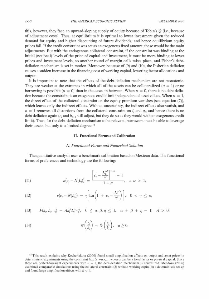
this, however, they face an upward-sloping supply of equity because of Tobin’s Q (i.e., because of adjustment costs). Thus, at equilibrium it is optimal to lower investment given the reduced demand for equity and higher discounting of future dividends, and hence equilibrium equity prices fall. If the credit constraint was set as an exogenous fixed amount, these would be the main adjustments. But with the endogenous collateral constraint, if the constraint was binding at the initial (notional) levels of the price of capital and investment, it must be more binding at lower prices and investment levels, so another round of margin calls takes place, and Fisher’s debt-deflation mechanism is set in motion. Moreover, because of (9) and (10), the Fisherian deflation causes a sudden increase in the financing cost of working capital, lowering factor allocations and output.

It is important to note that the effects of the debt-deflation mechanism are not monotonic. They are weaker at the extremes in which all of the assets can be collateralized (κ=1) or no borrowing is possible (κ=0) than in the cases in between. When κ=0, there is no debt defla-tion because the constraint is an exogenous credit limit independent of asset values. When κ=1, the direct effect of the collateral constraint on the equity premium vanishes (see equation (7)), which leaves only the indirect effects. Without uncertainty, the indirect effects also vanish, and κ=1 removes all distortions from the collateral constraint on it and qt, and hence there is no debt deflation again (ct and bt+1 still adjust, but they do so as they would with an exogenous credit limit). Thus, for the debt-deflation mechanism to be relevant, borrowers must be able to leverage their assets, but only to a limited degree.12

II. Functional Forms and Calibration

A. Functional Forms and Numerical Solution

The quantitative analysis uses a benchmark calibration based on Mexican data. The functional forms of preferences and technology are the following:

(11) u(ct − N(Lt)) = cct −

L t ω___ωd

1−σ

−1 _____________

1 − σ , σ, ω > 1,

(12) v(ct − N(Lt)) = γcLn a1 + ct − L t

ω___ωb d , 0 < γ ≤ σ,

(13) F(kt, Lt, vt) = A k t βL t

αv t η, 0 ≤ α, β, η ≤ 1, α + β + η = 1, A > 0,

(14) Ψ a zt __kt

b = a __2 a zt __

kt b , a ≥ 0.

12 This result explains why Kocherlakota (2000) found small amplification effects on output and asset prices in deterministic experiments using the constraint bt+1≥−qt xt+1, where x can be a fixed factor or physical capital. Since these are perfect-foresight experiments with κ=1, the debt-deflation mechanism is neutralized. Mendoza (2006) examined comparable simulations using the collateral constraint (3) without working capital in a deterministic set-up and found large amplification effects with κ < 1.


The utility and time preference functions in (11) and (12) are standard from DSGE-SOE models. The parameter σ is the coefficient of relative risk aversion, ω determines the wage elasticity of labor supply, which is given by 1/(ω − 1), and γ is the semielasticity of the rate of time preference with respect to composite good c − N(L). The restriction γ ≤ σ is a condition required to ensure that SCU supports a unique, invariant limiting distribution of bonds and capital (see Epstein 1983). The Cobb-Douglas technology (13) is the production function for gross output. Equation (14) is the net investment adjustment cost function.

B. Calibration

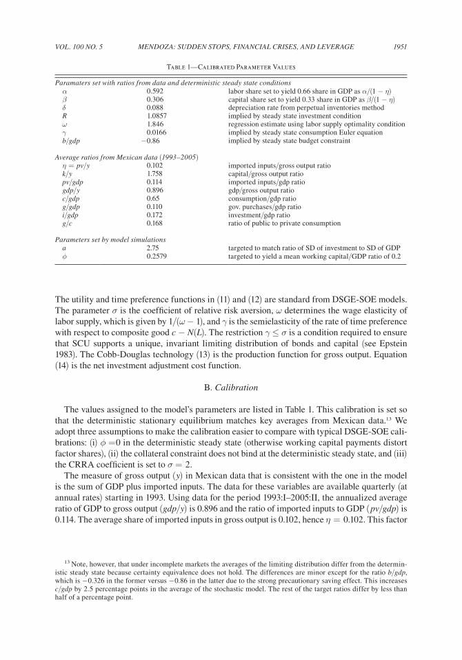
The values assigned to the model’s parameters are listed in Table 1. This calibration is set so that the deterministic stationary equilibrium matches key averages from Mexican data.13 We adopt three assumptions to make the calibration easier to compare with typical DSGE-SOE cali-brations: (i) ϕ =0 in the deterministic steady state (otherwise working capital payments distort factor shares), (ii) the collateral constraint does not bind at the deterministic steady state, and (iii) the CRRA coefficient is set to σ =2.

The measure of gross output (y) in Mexican data that is consistent with the one in the model is the sum of GDP plus imported inputs. The data for these variables are available quarterly (at annual rates) starting in 1993. Using data for the period 1993:I–2005:II, the annualized average ratio of GDP to gross output (gdp/y) is 0.896 and the ratio of imported inputs to GDP (pv/gdp) is 0.114. The average share of imported inputs in gross output is 0.102, hence η=0.102. This factor

13 Note, however, that under incomplete markets the averages of the limiting distribution differ from the determin-istic steady state because certainty equivalence does not hold. The differences are minor except for the ratio b/gdp, which is −0.326 in the former versus −0.86 in the latter due to the strong precautionary saving effect. This increases c/gdp by 2.5 percentage points in the average of the stochastic model. The rest of the target ratios differ by less than half of a percentage point.

Table 1—Calibrated Parameter Values

Paramaters set with ratios from data and deterministic steady state conditions α 0.592 labor share set to yield 0.66 share in GDP as α/(1 − η) β 0.306 capital share set to yield 0.33 share in GDP as β/(1 − η) δ 0.088 depreciation rate from perpetual inventories method R 1.0857 implied by steady state investment condition ω 1.846 regression estimate using labor supply optimality condition γ 0.0166 implied by steady state consumption Euler equation b/gdp −0.86 implied by steady state budget constraint

Average ratios from mexican data (1993–2005) η=pv/y 0.102 imported inputs/gross output ratio k/y 1.758 capital/gross output ratio pv/gdp 0.114 imported inputs/gdp ratio gdp/y 0.896 gdp/gross output ratio c/gdp 0.65 consumption/gdp ratio g/gdp 0.110 gov. purchases/gdp ratio i/gdp 0.172 investment/gdp ratio g/c 0.168 ratio of public to private consumption

Parameters set by model simulations a 2.75 targeted to match ratio of SD of investment to SD of GDP ϕ 0.2579 targeted to yield a mean working capital/GDP ratio of 0.2


share, combined with the 0.66 labor share on GDP from Rodrigo García-Verdú (2005) implies the following factor shares: α=(0.66/(1 + (pv/gdp))=0.592 and β =1 − α − η=0.306.14

We also use García-Verdú’s (2005) estimates of Mexico’s capital stock, together with our mea-sure of y, to construct an estimate of the capital–gross output ratio (k/y) and to set the value of the depreciation rate. He used annual National Accounts investment data for the period 1950–2000 and the perpetual inventories method to construct a time series of the capital-GDP ratio. The average capital-GDP ratio for 1980–2000 is 1.88 with a 1980 point estimate of 1.56. Using these annual benchmarks, we constructed a quarterly capital stock series compatible with the quar-terly gross output estimates (starting in 1980 because quarterly investment data, again at annual rates, are available as of 1980:I). The annualized quarterly capital stock estimates match García-Verdú’s annual benchmarks by setting the initial capital-GDP ratio to 1.45 and the depreciation rate to 8.8 percent per year. The 1980:I–2005:II average of k/y is 1.758. Combined with the 0.088 depreciation rate, this value of k/y yields an average investment–gross output ratio (i/y) of 15.5 percent.

The value of p in the deterministic stationary state is set equal to the ratio of the averages of the ratios of imported inputs to gross output at current and constant prices, which is 1.028. The value of the annual gross real interest rate is set by imposing the values of β, (i/y), and δ on the Euler equation for capital evaluated at steady state and solving for R. The resulting expression yields R =1 + [δ(β−(i/y))]/(i/y)=1.086. A real interest rate of 8.6 percent is relatively high, but in this calibration it represents the implied real interest rate that, given the values of δ and β, supports Mexico’s average investment–gross output ratio as a feature of the deterministic steady state of a standard SOE model. Note also that with this calibration strategy the deterministic steady state matches Mexico’s average investment-GDP ratio of 17.2 percent.

The model’s optimality condition for labor supply equates the marginal disutility of labor with the real wage, which at equilibrium is equal to the marginal product of labor. This condition reduces to: L t

ω=αexp(ε t A )F (·). Using the logarithm of this expression, our estimate of gross

output, and Mexican data on employment growth, the implied value of the exponent of labor supply in utility is ω = 1.846. This value is similar to those typically used in DSGE-SOE models (e.g., Mendoza 1991, Uribe and Yue 2006).

Since aggregate demand in the data includes government expenditures, the model needs an adjustment to consider these purchases in order for the deterministic steady state to match the actual average private consumption-GDP ratio of 0.65. This adjustment is done by setting the deterministic steady state to match the observed average ratio of government purchases to GDP (0.11), assuming that these government purchases are unproductive and paid out of a time-invari-ant, ad valorem consumption tax. The tax is equal to the ratio of the GDP shares of government and private consumption, 0.11/0.65 =0.168, which is very close to the statutory value-added tax rate in Mexico. Since this tax is time invariant, it does not distort the intertemporal decision mar-gins and any distortion on the consumption-leisure margin does not vary over the business cycle.

Given the preference and technology parameters set in the previous paragraphs, the optimality conditions for L and v and the steady-state Euler equation for capital are solved as a nonlinear simultaneous equation system to determine the steady-state levels of k, L, and v. Given these, the levels of gross output and GDP are computed using the production function and the definition of GDP, and the level of consumption is determined by multiplying GDP times the average con-sumption-GDP ratio in the data. The value of γ follows then from the steady-state consumption Euler equation, which yields γ=ln(R)/ln(1 + c − ω−1Lω)=0.0166. As is typical in calibration exercises with SCU preferences (see Mendoza 1991), the value of the time preference coefficient

14 The share of labor income in GDP is about one-third in National Accounts data, but García-Verdú showed that in household survey data the share is about two-thirds, in line with standard estimates.


is very low, suggesting that the “impatience effects” introduced by the endogenous rate of time preference have negligible quantitative implications. Finally, the steady-state foreign asset posi-tion follows from the budget constraint (equation (2)) evaluated at steady state. This implies a ratio of net foreign assets to GDP of about −0.86.

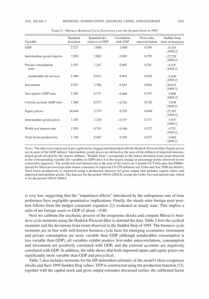
Next we calibrate the stochastic process of the exogenous shocks and compute Mexico’s busi-ness cycle moments using the Hodrick-Prescott filter to detrend the data. Table 2 lists the cyclical moments and the deviations from trend observed in the Sudden Stop of 1995. The business cycle moments are in line with well-known business cycle facts for emerging economies: investment and private consumption are more variable than GDP (although nondurables consumption is less variable than GDP), all variables exhibit positive first-order autocorrelations, consumption and investment are positively correlated with GDP, and the external accounts are negatively correlated with GDP. In addition, the table shows that both imported inputs and equity prices are significantly more variable than GDP and procyclical.

Table 2 also includes moments for the HP-detrended estimates of the model’s three exogenous shocks and their 1995 Sudden Stop values. TFP is constructed using the production function (13), together with the capital stock and gross output estimates discussed earlier, the calibrated factor

Table 2—Mexico: Business Cycle Statistics and the Sudden Stop of 1995

Standard Standard dev. Correlation First-order Sudden Stop Variable deviation relative to GDP with GDP autocorrelation (date in brackets)GDP 2.723 1.000 1.000 0.749 −8.315

(1995:2)Intermediate goods imports 7.850 2.882 0.905 0.759 −27.229

(1995:2)Private consumption 3.397 1.247 0.895 0.701 −8.175 total (1995:3)

nondurables & services 2.490 0.914 0.893 0.676 −5.649(1995:2)

Investment 9.767 3.586 0.944 0.816 −30.074(1995:3)

Net exports–GDP ratio 2.109 0.775 −0.688 0.797 4.898(1995:2)

Current account–GDP ratio 1.560 0.573 −0.754 0.720 3.838(1995:2)

Equity prices 14.648 5.379 0.570 0.640 −27.397(1995:2)

Intermediate goods prices 3.345 1.228 −0.377 0.737 5.915(1995:1)

World real interest rate 1.958 0.719 −0.590 0.572 6.752(1995:2)

Total factor productivity 1.340 0.492 0.519 0.537 −5.082(1995:2)

Notes: The data were expressed in per capita terms, logged and detrended with the Hodrick-Prescott filter. Equity prices are in units of the GDP deflator. Intermediate goods prices are defined as the ratio of the deflator of imported interme-diated goods divided by the exports deflator. “Sudden Stop” corresponds to the lowest deviation from trend observed in the corresponding variable (for variables in GDP ratios it is the largest change in percentage points observed in two consecutive quarters). The world real real interest rate is the sum of the return on 3-month US T bills plus the EMBI+ spread for Mexican sovereign debt minus a measure of expected US CPI inflation (see Uribe and Yue 2006 for details). Total factor productivity is measured using a production function for gross output that includes capital, labor, and imported intermediate goods. The data are for the period 1993:I–2005:II, except the Uribe-Yue real interest rate, which is for the period 1994:I–2004:I.


shares, and data on L and v (see Mendoza 2006 for details). The relative price of imported inputs is the deflator of imported inputs divided by the exports deflator (which removes effects from changes in the nominal exchange rate or in nontradables prices). The real interest rate is Uribe and Yue’s (2006) measure of Mexico’s real interest rate in world capital markets. Note that the 1995 Sudden Stop coincided with sizable shocks, but we will show below that Sudden Stops are possible in the model even with one–standard deviation shocks. Also, typical endogeneity cave-ats apply to the estimates of εR, because of the link between country risk and business cycles, and εA, because of factors that bias measured TFP in addition to imported inputs (e.g., capacity utilization, factor hoarding). As a result, the large shocks shown for the 1995 Sudden Stop may overestimate the true exogenous shocks that occurred that year.

The shocks are modeled as a joint discrete Markov process that approximates the statistical moments of their actual time-series processes. The Markov process is defined by a set E of all combinations of realizations of the shocks, each combination given by a triple e =(ε A, εR, εP ), and by a matrix π of transition probabilities of moving from et to et+1. In the data, εA, εR, and εP are AR(1) processes with standard deviations and first-order autocorrelations as reported in the last three rows of Table 2. Since the three shocks are nearly independent, except for a sta-tistically significant correlation between εR and εA of about −0.67, the Markov process is con-structed using the parsimonious structure of the two-point, symmetric simple persistence rule as in Mendoza (1995). Each shock has two realizations equal to plus/minus one standard deviation of each shock in the data (ε1

A = − ε2

A =0.0134, ε1

R =− ε2

R =0.0196, ε1

P =−ε2

P =0.0335), so

E contains eight triples. The simple persistence rule produces an 8×8 matrix π which yields autocorrelations of the shocks and a correlation between εA and εR that match those in the data. The procedure requires, however, that the AR(1) coefficients of the shocks that are correlated with each other (εA and εR ) be the same—which is in line with the data where ρ(ε R )=0.572 and ρ(ε A )=0.537.

Two parameter values remain to be determined: the adjustment cost coefficient a and the working capital coefficient ϕ. We set these so that the model matches the observed ratio of the standard deviation of Mexico’s gross investment relative to GDP (3.6) and a mean ratio of work-ing capital to GDP of 1/5, both in a model simulation where the collateral constraint does not bind. This yields a =2.75 and ϕ =0.26.15 This is a reasonable approach to calibrate a because this parameter does not affect the deterministic steady state, but it affects the variability of investment. The working capital-GDP target of 20 percent is an approximation to actual data. Data on working capital financing for Mexico are not available, but the 1994:I–2005:I average of total credit to private nonfinancial firms as a share of GDP was 24.4 percent. Note, however, that this measure includes credit at all maturities and for all uses, so it overestimates actual working capital financing. On the other hand, these data include the 1995–2002 period in which Mexican banks were being recapitalized after the 1994 crisis, and credit declined sharply for “abnormal” reasons that may bias the average credit-output ratio downwards.

One important observation is that ϕ =0.26 is much lower than the working capital coefficients used by Neumeyer and Perri (2005) and Uribe and Yue (2006). As Oviedo (2004) showed, with low working capital coefficients, the working capital channel has very weak effects on business cycle moments. Hence, the role of working capital in this model is limited to the amplification and asymmetry that it contributes to when the collateral constraint binds. Its effect on regular business cycle volatility is negligible.

15 Given this low value of ϕ and that R − 1 =0.0857, setting ϕ =0 in solving the deterministic steady state to calibrate the other parameters makes very little difference and keeps the calibration comparable with those in the quantitative literature on DSGE-SOE models.


III. Results of the Quantitative Analysis

The model is solved by representing the equilibrium in recursive form and using a nonlinear global solution method with the collateral constraint imposed as an occasionally binding con-straint. The endogenous state variables are k and b. These are chosen from evenly spaced dis-crete grids of NK values of capital, K ={k1 < k2 < … < kNK}, and NB bond positions, B ={b1 < b2 < … < bNB}. Hence, the state space is defined by all triples (k, b, e)∈K×B×E. We set NK =60 and NB =80, so the state space of the model has 60×80×8 coordinates. The solution method produces decision rules for kt+1 and bt+1 as functions of (kt, bt, et). These decision rules and the transition matrix π are then used to iterate to convergence on the long-run probability distribution P(k, b, e) of observing each coordinate (k, b, e)∈K×B×E at any given date t. This stochastic steady state is used to compute business cycle moments and averages of amplification coefficients, as explained later in this section. The NBER working paper version of Mendoza and Smith (2006) provides further details on algorithms for solving models with collateral con-straints linked to asset prices (see http://www.nber.org/papers/w10940). Given their finding that the externality resulting from the representative agent ignoring the implications of its actions for asset prices in the collateral constraint is small, the model is solved using their “quasi social planner” algorithm.

A. Long-Run Business Cycle moments

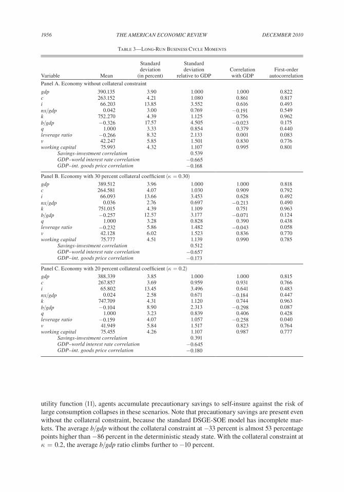
The first important result is that long-run business cycle moments are largely unaffected by the collateral constraint. Looking at Table 3, the moments of the economy without collateral constraints (panel A) are very similar to those from two scenarios in which the constraint binds in some states of nature (panels B with κ=0.3 and C with κ=0.2). The scenario with κ=0.2 is the baseline that matches the observed frequency of Sudden Stops (see subsection B below), and κ=0.3 is shown for comparison.

Panel A shows that the model does well at accounting for Mexico’s business cycle facts. The model overestimates the variability of GDP (3.9 percent in the model versus 2.7 percent in the data), but scaling by the variability of output the model does a fair job at matching the variability of the other variables, and the GDP-correlations and first-order autocorrelations are generally in line with the data. The model does particularly well at accounting for three moments that the literature on emerging markets business cycles emphasizes: consumption is more variable than GDP, the interest rate and GDP are negatively correlated, and net exports are countercyclical. Moreover, contrary to the findings of Javier Garcia Cicco, Roberto Pancrazi, and Uribe (forth-coming), the model does not yield near–unit root behavior in the net exports–GDP ratio—the first-order autocorrelation of this ratio is 0.549 in the model versus 0.797 in the data. This sug-gests that their result can be a miscalculation of the perturbation method they used. Near–unit root behavior in net exports is not a feature of the “exact” solution of the RBC-SOE model obtained with a global method.

Panels B and C show that the only marked differences in long-run business cycles in econo-mies with and without the collateral constraint are on the moments directly influenced by it (the leverage ratio and the ratios of foreign assets and net exports to GDP). The means of the leverage and foreign assets ratios rise, and the mean of the net exports–GDP ratio falls, the variability of the three declines, and all three become more countercyclical.

The key feature of the model behind the result that long-run business cycle moments are largely unaffected by the collateral constraint is the precautionary savings motive. The high-leverage states at which the credit constraint binds are reached after cyclical dynamics in response to histories of shocks lead the leverage ratio to hit its ceiling. Because of the curvature of the


utility function (11), agents accumulate precautionary savings to self-insure against the risk of large consumption collapses in these scenarios. Note that precautionary savings are present even without the collateral constraint, because the standard DSGE-SOE model has incomplete mar-kets. The average b/gdp without the collateral constraint at −33 percent is almost 53 percentage points higher than −86 percent in the deterministic steady state. With the collateral constraint at κ=0.2, the average b/gdp ratio climbs further to −10 percent.

Table 3—Long-Run Business Cycle Moments

Variable Mean

Standarddeviation

(in percent)

Standarddeviation

relative to GDPCorrelationwith GDP

First-orderautocorrelation

Panel A. Economy without collateral constraint

gdp 390.135 3.90 1.000 1.000 0.822c 263.152 4.21 1.080 0.861 0.817i 66.203 13.85 3.552 0.616 0.493nx/gdp 0.042 3.00 0.769 −0.191 0.549k 752.270 4.39 1.125 0.756 0.962b/gdp −0.326 17.57 4.505 −0.023 0.175q 1.000 3.33 0.854 0.379 0.440leverage ratio −0.266 8.32 2.133 0.001 0.083v 42.247 5.85 1.501 0.830 0.776working capital 75.993 4.32 1.107 0.995 0.801

Savings-investment correlation 0.539GDP–world interest rate correlation −0.665GDP–int. goods price correlation −0.168

Panel B. Economy with 30 percent collateral coefficient (κ= 0.30)gdp 389.512 3.96 1.000 1.000 0.818c 264.581 4.07 1.030 0.909 0.792i 66.093 13.66 3.453 0.628 0.492nx/gdp 0.036 2.76 0.697 −0.213 0.490k 751.015 4.39 1.109 0.751 0.963b/gdp −0.257 12.57 3.177 −0.071 0.124q 1.000 3.28 0.828 0.390 0.438leverage ratio −0.232 5.86 1.482 −0.043 0.058v 42.128 6.02 1.523 0.836 0.770working capital 75.777 4.51 1.139 0.990 0.785


Panel C. Economy with 20 percent collateral coefficient (κ= 0.2)gdp 388.339 3.85 1.000 1.000 0.815c 267.857 3.69 0.959 0.931 0.766i 65.802 13.45 3.496 0.641 0.483nx/gdp 0.024 2.58 0.671 −0.184 0.447k 747.709 4.31 1.120 0.744 0.963b/gdp −0.104 8.90 2.313 −0.298 0.087q 1.000 3.23 0.839 0.406 0.428leverage ratio −0.159 4.07 1.057 −0.258 0.040v 41.949 5.84 1.517 0.823 0.764working capital 75.455 4.26 1.107 0.987 0.777



B. Amplification and Asymmetry with the Collateral Constraint

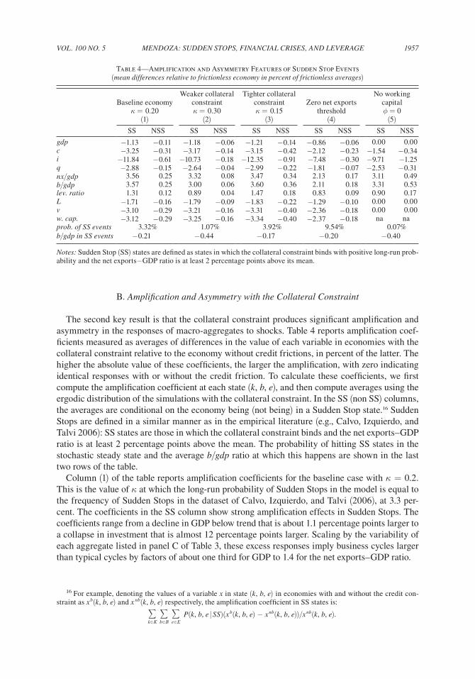
The second key result is that the collateral constraint produces significant amplification and asymmetry in the responses of macro-aggregates to shocks. Table 4 reports amplification coef-ficients measured as averages of differences in the value of each variable in economies with the collateral constraint relative to the economy without credit frictions, in percent of the latter. The higher the absolute value of these coefficients, the larger the amplification, with zero indicating identical responses with or without the credit friction. To calculate these coefficients, we first compute the amplification coefficient at each state (k, b, e), and then compute averages using the ergodic distribution of the simulations with the collateral constraint. In the SS (non SS) columns, the averages are conditional on the economy being (not being) in a Sudden Stop state.16 Sudden Stops are defined in a similar manner as in the empirical literature (e.g., Calvo, Izquierdo, and Talvi 2006): SS states are those in which the collateral constraint binds and the net exports–GDP ratio is at least 2 percentage points above the mean. The probability of hitting SS states in the stochastic steady state and the average b/gdp ratio at which this happens are shown in the last two rows of the table.

Column (1) of the table reports amplification coefficients for the baseline case with κ=0.2. This is the value of κ at which the long-run probability of Sudden Stops in the model is equal to the frequency of Sudden Stops in the dataset of Calvo, Izquierdo, and Talvi (2006), at 3.3 per-cent. The coefficients in the SS column show strong amplification effects in Sudden Stops. The coefficients range from a decline in GDP below trend that is about 1.1 percentage points larger to a collapse in investment that is almost 12 percentage points larger. Scaling by the variability of each aggregate listed in panel C of Table 3, these excess responses imply business cycles larger than typical cycles by factors of about one third for GDP to 1.4 for the net exports–GDP ratio.

16 For example, denoting the values of a variable x in state (k, b, e) in economies with and without the credit con-straint as x b(k, b, e) and x nb(k, b, e) respectively, the amplification coefficient in SS states is:

∑k∈K

∑b∈B

∑e∈E

P(k, b, e |SS)(x b(k, b, e) − x nb(k, b, e))/x nb(k, b, e).

Table 4—Amplification and Asymmetry Features of Sudden Stop Events (mean differences relative to frictionless economy in percent of frictionless averages)

Baseline economyκ =0.20

(1)

Weaker collateral constraintκ =0.30

(2)

Tighter collateral constraintκ =0.15

(3)

Zero net exportsthreshold

(4)

No working capitalϕ = 0(5)

SS NSS SS NSS SS NSS SS NSS SS NSS

gdp −1.13 −0.11 −1.18 −0.06 −1.21 −0.14 −0.86 −0.06 0.00 0.00c −3.25 −0.31 −3.17 −0.14 −3.15 −0.42 −2.12 −0.23 −1.54 −0.34i −11.84 −0.61 −10.73 −0.18 −12.35 −0.91 −7.48 −0.30 −9.71 −1.25q −2.88 −0.15 −2.64 −0.04 −2.99 −0.22 −1.81 −0.07 −2.53 −0.31nx/gdp 3.56 0.25 3.32 0.08 3.47 0.34 2.13 0.17 3.11 0.49b/gdp 3.57 0.25 3.00 0.06 3.60 0.36 2.11 0.18 3.31 0.53lev. ratio 1.31 0.12 0.89 0.04 1.47 0.18 0.83 0.09 0.90 0.17L −1.71 −0.16 −1.79 −0.09 −1.83 −0.22 −1.29 −0.10 0.00 0.00v −3.10 −0.29 −3.21 −0.16 −3.31 −0.40 −2.36 −0.18 0.00 0.00w. cap. −3.12 −0.29 −3.25 −0.16 −3.34 −0.40 −2.37 −0.18 na naprob. of SS events 3.32% 1.07% 3.92% 9.54% 0.07%b/gdp in SS events −0.21 −0.44 −0.17 −0.20 −0.40

Notes: Sudden Stop (SS) states are defined as states in which the collateral constraint binds with positive long-run prob-ability and the net exports−GDP ratio is at least 2 percentage points above its mean.


The asymmetry of the amplification effects is illustrated by the stark comparison of the ampli-fication coefficients across the SS and non-SS columns. The amplification coefficients in non-SS states are very small, indicating that variables respond about the same with the collateral constraint as without it, and scaling by the variability of each aggregate the difference across the two is negligible. Since Sudden Stops are low probability events in the long run, the moments shown in Table 3 reflect mainly these non-SS states where there is almost no amplification due to the credit constraint, which explains the previous finding showing that business cycle moments with or without the collateral constraint are very similar. An important implication of this result is that relatively rare Sudden Stops coexist with the more frequent, normal business cycles sum-marized in the moments of Table 3.

It is also worth noting that the responses in the SS and non-SS columns are produced by shocks that are at most one standard deviation in size, and that the shocks hitting the economies with and without the collateral constraint in each of the two columns of the table are identical. Thus, the model displays significant amplification and asymmetry in response to shocks that are relatively small, and it has the feature that symmetric shocks produce asymmetric responses.

Columns (2) to (5) of Table 4 show that the result indicating that the collateral constraint induces significant amplification and asymmetry is robust to several parameter changes. Columns (2) and (3) report results for κ=0.3 and κ=0.15 respectively. Column (4) lowers the net exports–GDP threshold ratio used to define Sudden Stops from an increase of 2 percentage points above the mean to zero. Column (5) removes working capital financing by setting ϕ =0.

Increasing (reducing) κ has small effects on most amplification coefficients, but it reduces (increases) the amplification effect on the leverage ratio and the probability of Sudden Stops. Lowering the net exports–GDP threshold to zero weakens the amplification coefficients some-what, but again the largest effect is on the probability of Sudden Stops, which rises sharply when the threshold used to define them is lowered significantly. Still, in all these scenarios there is significant amplification and asymmetry.

Removing working capital does change the results significantly. In particular, the model can-not generate any amplification in GDP and factor allocations, and the probability of Sudden Stops (keeping κ=0.2) is much lower than in the baseline. These results are due to the fact that, without working capital, factor allocations and output cannot be affected contemporaneously by the collateral constraint. In conditions (9) and (10), capital is predetermined and the external financing premium due to the binding collateral constraint is no longer present, and as a result (9) and (10) together with the labor supply condition (wt =N′(Lt)) determine identical allocations for labor, intermediate goods, and output regardless of whether the constraint binds or not.17 Hence, these variables take identical values at each state (k, b, e) with and without the constraint, which implies zero amplification coefficients for all (k, b, e). The rest of the macro-aggregates continue to display significant amplification and asymmetry, although the amplification coefficients are smaller than in the scenarios shown in the other columns.

C. Can the model Explain Observed Sudden Stop Events?

The simulations can also be used to evaluate the model’s ability to account for the actual dynamics of Sudden Stop events in Figure 1. To this end, we conduct a 10,000-period stochastic time-series simulation and use the simulated data to construct five-year event windows centered

17 This result hinges on the assumption that there is no wealth effect on labor supply. Without it, the tilting of con-sumption imposed by the borrowing constraint would distort labor supply.


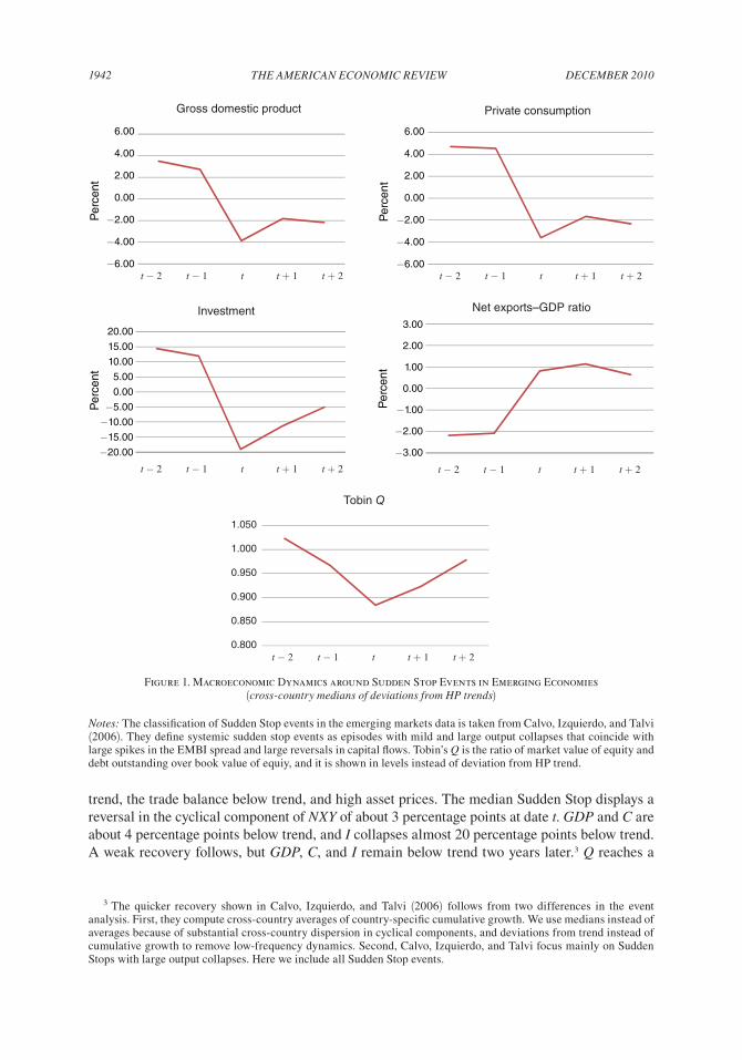
on SS events.18 Figure 2 shows the windows for GDP, C, I, Tobin’s Q, and NXY, as well as for the shocks on TFP, imported input prices, and the interest rate. To match the methodology used in Figure 1, each window includes the median across SS events identified in the 10,000 period

18 These event windows capture dynamic effects beyond the initial impact effects captured in amplification coeffi-cients. For example, the drop in It when a Sudden Stop hits has a negative effect on GDPt+1 that is captured in the event window but not in the amplification coefficient. Alternatively, the dynamic effects can be illustrated using conditional impulse responses or cumulative amplification effects starting from an initial Sudden Stop as in Mendoza (2006).

Gross domestic product

model +1SD -1SD data Mexico

Private consumption

model data Mexico

Investment

model data Mexico


model data Mexico

−

Tobin Q

model data

Exogenous shocks

TFP Interest rate Price of imported inputs

+1SD 1SD−

+1SD 1SD−

+1SD 1SD−

+1SD 1SD−

t − 2 t − 1 t t + 1 t + 2 t − 2 t − 1 t t + 1 t + 2

t − 2 t − 1 t t + 1 t + 2

t − 2 t − 1 t t + 1 t + 2t − 2 t − 1 t t + 1 t + 2

t − 2 t − 1 t t + 1 t + 2

0.06

0.04

0.02

0

−0.02

−0.04

−0.06

0.08

0.06

0.04

0.02

0

−0.02

−0.04

−0.06

0.3

0.2

0.1

0

−0.1

−0.2

−0.3

0.060.050.040.030.020.01

0−0.01−0.02−0.03−0.04−0.05

0.0250.02

0.0150.01

0.0050

−0.005−0.01−0.015−0.02−0.025

1.1

1.05

1

0.95

0.9

0.85

0.8

Figure 2. Sudden Stop Event Windows in Actual Data and Model Simulations (medians of deviations from HP trends)

Notes: Event from actual data are as in Figure 1, which uses the definitions from Calvo, Izquierdo, and Talvi (2006). Mexican data are for the Sudden Stop of 1995. Sudden Stop events in the model simulations are defined in a manner analogous to Calvo, Izquierdo, and Talvi, as events in which the collateral constraint binds, output is at least one stan-dard deviation below trend, and the trade balance–GDP ratio is at least one standard deviation above trend. Tobin’s Q is shown in levels.


simulation. We also include for comparison one–standard deviation bands, the actual event win-dow observations from Figure 1, and the observations from Mexico’s 1995 Sudden Stop. To be consistent with Calvo, Izquierdo, and Talvi’s (2006) definition of systemic SS events with mild and large output collapses, a Sudden Stop event is identified as a situation in which the collateral constraint binds, GDP is at least one standard deviation below trend, and NXY is at least one standard deviation above trend.

Figure 2 shows that the model replicates most of the key features of actual SS events, except for the magnitude of the decline in asset prices. The model predicts that Sudden Stops are pre-ceded by periods of expansion, with GDP, C, and I above trend and NXY running deficits at t − 2 and t − 1. In the date of the SS events (date t), the model matches closely the magnitude of the declines in GDP, C, and I. The reversal in NXY between t − 1 and t is also very similar to the one in the data, but the levels in the model overestimate those in the data. The model is also consis-tent with the data in predicting a weak recovery in dates t + 1 and t + 2. With regard to Tobin’s Q, the model’s dynamics are qualitatively correct, but quantitatively the decline in asset prices is about 40 percent the size of the actual decline. Relative to the Mexican SS event, the model again matches very well the magnitude of the declines in GDP and C at date t, but it underestimates the pre–Sudden Stop boom and the size of the reversal in NXY.

Figure 2 also shows that the median Sudden Stop in the model is preceded by low interest rates, about 2 percent below the long-run mean, with TFP and imported input prices above trend by small margins. Hence, interest rate shocks play a more important role than the other shocks in driving the increase of the leverage ratio before a Sudden Stop. In Sudden Stop events them-selves, however, all three shocks turn unfavorable. Between t − 1 and t, the interest rate surges by 4 percentage points, TFP declines by nearly 2 percentage points, and the price of imported inputs rises by half of a percentage point.

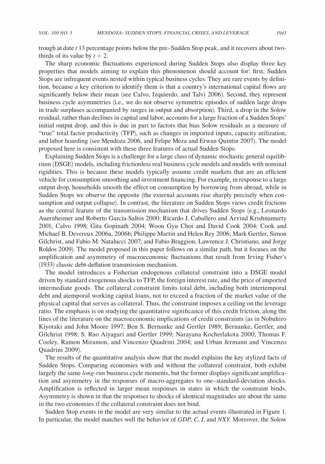
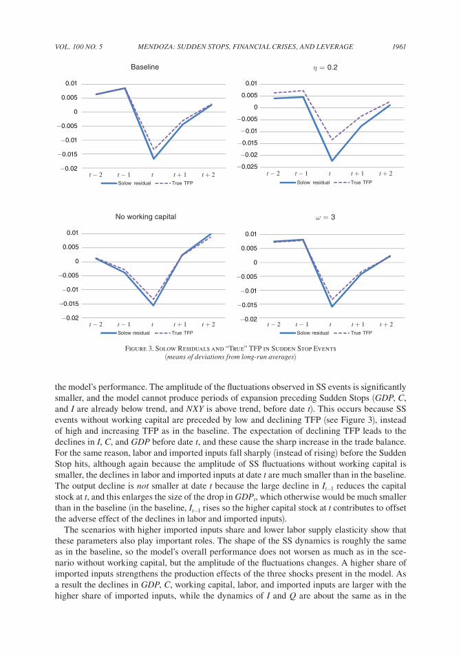
Figure 3 shows event windows for “true” TFP (i.e., εA ) and for the model’s Solow residual, defined as s ≡ gdp/(k β/(1−η)Lα/(1−η)). In the baseline scenario with κ=0.2, the two are very similar except on the date of SS events, when the Solow residual falls more than true TFP. Thus, the model is also consistent with the data in predicting that part of the decline in GDP observed during SS events cannot be accounted for by changes in measured capital and labor, and that this decline in the Solow residual overestimates actual TFP (albeit the difference is not large). However, it is also important to acknowledge that a 1.5 percent negative TFP shock is still needed for the output decline to be realistic, and the reason for this decline remains an open question beyond the scope of this paper.

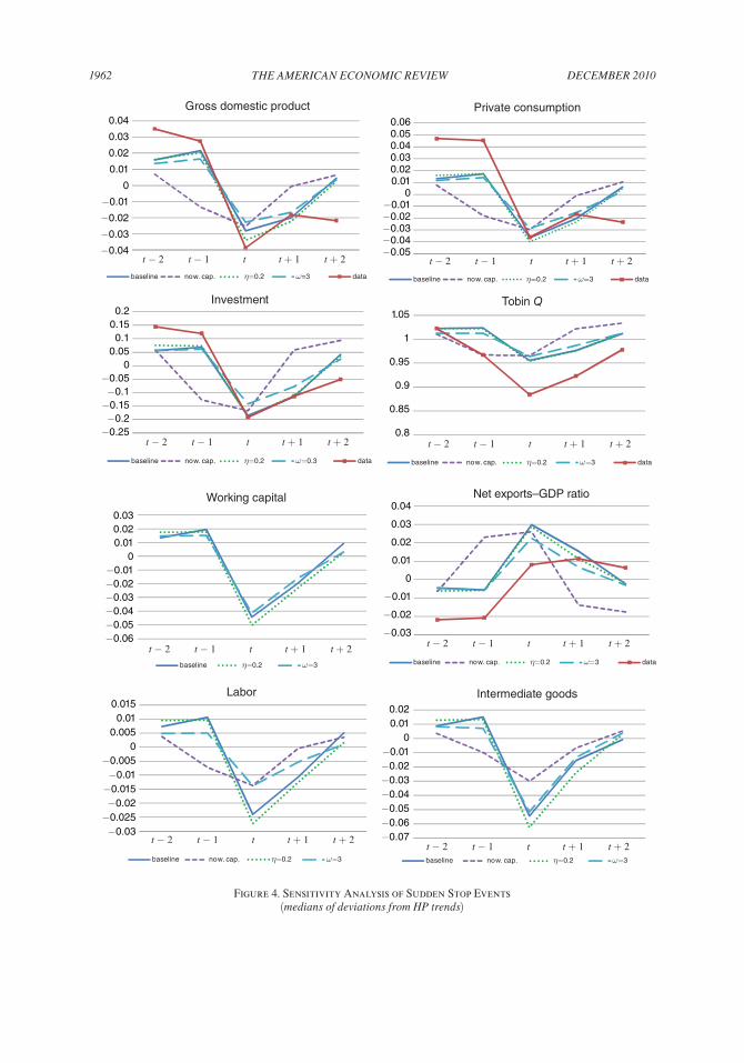
D. Sensitivity Analysis of Sudden Stop Event Windows

Figure 4 compares Sudden Stop events in the baseline economy with κ=0.2 with those of three alternative scenarios: (i) no working capital (ϕ=0), (ii) higher share of imported inputs in production (η=0.2 versus 0.1 in the baseline), and (iii) lower labor supply elasticity (0.5 instead of 1.2, which implies ω=3 instead of 1.85). The figure also includes the actual event dynam-ics for comparison. Figure 3 compares the event windows of Solow residuals versus true TFP in the same three scenarios and the baseline. Note that we consider relatively small changes in parameters because otherwise the economies differ sharply in debt and leverage dynamics, and this requires recalibrating κ in order to study the effects of the occasionally binding collateral constraint. With the parameter changes we study here, the value of κ can remain at 20 percent in all scenarios.

The model without working capital performs much worse than all of the alternatives in terms of its ability to account for Sudden Stop dynamics, reaffirming the previous finding indicating that the cutoff in access to working capital when the collateral constraint binds is important for


the model’s performance. The amplitude of the fluctuations observed in SS events is significantly smaller, and the model cannot produce periods of expansion preceding Sudden Stops (GDP, C, and I are already below trend, and NXY is above trend, before date t). This occurs because SS events without working capital are preceded by low and declining TFP (see Figure 3), instead of high and increasing TFP as in the baseline. The expectation of declining TFP leads to the declines in I, C, and GDP before date t, and these cause the sharp increase in the trade balance. For the same reason, labor and imported inputs fall sharply (instead of rising) before the Sudden Stop hits, although again because the amplitude of SS fluctuations without working capital is smaller, the declines in labor and imported inputs at date t are much smaller than in the baseline. The output decline is not smaller at date t because the large decline in It−1 reduces the capital stock at t, and this enlarges the size of the drop in GDPt, which otherwise would be much smaller than in the baseline (in the baseline, It−1 rises so the higher capital stock at t contributes to offset the adverse effect of the declines in labor and imported inputs).

The scenarios with higher imported inputs share and lower labor supply elasticity show that these parameters also play important roles. The shape of the SS dynamics is roughly the same as in the baseline, so the model’s overall performance does not worsen as much as in the sce-nario without working capital, but the amplitude of the fluctuations changes. A higher share of imported inputs strengthens the production effects of the three shocks present in the model. As a result the declines in GDP, C, working capital, labor, and imported inputs are larger with the higher share of imported inputs, while the dynamics of I and Q are about the same as in the

Baseline

Solow residual True TFP

-

-

No working capital


η = 0.2


ω = 3


t − 2 t − 1 t t + 1 t + 2 t − 2 t − 1 t t + 1 t + 2

t − 2 t − 1 t t + 1 t + 2 t − 2 t − 1 t t + 1 t + 2

0.01

0.005

0

−0.005

−0.01

−0.015

−0.02

0.01

0.005

0

−0.005

−0.01

−0.015

−0.02

0.01

0.005

0

−0.005

−0.01

−0.015

−0.02

0.01

0.005

0

−0.005

−0.01

−0.015

−0.02

−0.025

Figure 3. Solow Residuals and “True” TFP in Sudden Stop Events (means of deviations from long-run averages)


Gross domestic product

baseline no w. cap. η=0.2 ω=3 data

Private consumption


Investment

baseline no w. cap. η=0.2 ω=0.3 data

Tobin Q




Labor

baseline no w. cap. η=0.2 ω=3

Intermediate goods

baseline no w. cap. η=0.2 ω=3

Working capital

baseline η=0.2 ω=3

t − 2 t − 1 t t + 1 t + 2 t − 2 t − 1 t t + 1 t + 2

t − 2 t − 1 t t + 1 t + 2t − 2 t − 1 t t + 1 t + 2

t − 2 t − 1 t t + 1 t + 2 t − 2 t − 1 t t + 1 t + 2

t − 2 t − 1 t t + 1 t + 2t − 2 t − 1 t t + 1 t + 2

0.04

0.03

0.02

0.01

0

−0.01

−0.02

−0.03

−0.04

0.060.050.040.030.020.01

0−0.01−0.02−0.03−0.04−0.05

0.20.150.1

0.050

−0.05−0.1−0.15−0.2−0.25

1.05

1

0.95

0.9

0.85

0.8

0.030.020.01

0−0.01−0.02−0.03−0.04−0.05−0.06

0.04

0.03

0.02

0.01

0

−0.01

−0.02

−0.03

0.020.01

0−0.01−0.02−0.03−0.04−0.05−0.06−0.07

0.0150.01

0.0050

−0.005−0.01−0.015−0.02−0.025−0.03

Figure 4. Sensitivity Analysis of Sudden Stop Events (medians of deviations from HP trends)


baseline. The fit with the data actually improves, because the drops in GDPt and Ct are nearly a perfect match to actual SS events. In addition, the higher imported inputs share creates a larger wedge between the Solow residual and true TFP (see Figure 3). A mean decline of about 1.2 per-cent in true TFP when Sudden Stops hit translates into a mean decline in the Solow residual that is almost twice as large.

The above results for higher η are important because the calibrated value of η=0.1 is prob-ably conservative. Evidence from countries other than Mexico suggests that imported inputs can have much higher shares. Linda S. Goldberg and José Manuel Campa (forthcoming) report ratios of imported inputs to total intermediate goods for 17 industrial countries that vary from 14 to 49 percent, with a median of 23 percent (the ratio for Mexico is about ¼). Moreover, to the extent that domestically produced inputs are substitutes for imported inputs, and purchases of domestic inputs require working capital financing, the scenario with the higher η is likely to be closer to the one that is empirically relevant, because domestic inputs would respond to a similar amplification mechanism to the one affecting imported inputs.19

The simulation with lower labor supply elasticity retains the same overall qualitative features of the baseline simulation: SS events are preceded by periods of expansion and followed by weak recoveries. With the weakened response of labor supply, however, the amplitude of the fluctua-tions is smaller, and the gap between true TFP and the Solow residual when the Sudden Stop hits is narrower, so the model does not do as well at matching the dynamics observed in the data. In contrast with the scenario that changed the share of imported inputs, lowering the labor supply elasticity does affect the behavior of investment and asset prices, both of which exhibit smaller declines than in the baseline scenario. Thus, these results show that labor supply elasticity of about 1.2, as in the baseline, or higher is important for the model’s ability to explain observed SS dynamics.

Mendoza (2006) conducted two additional sensitivity experiments that are worth noting.20 The first experiment demonstrates the importance of the debt-deflation channel by comparing amplification effects between a model with the Fisherian collateral constraint and an economy with a constant borrowing limit, set equal to the largest total debt (in bonds and working capital) attained with the Fisherian constraint. This change weakens the amplification effect on Q by a factor of 5.75 (from −6.9 percent with the Fisherian constraint to −1.2 with the constant debt limit), and that for I by a factor of 7.2 (−33 percent versus −4.6 percent). The second experiment studies amplification effects for each of the three shocks individually. In line with the results of the event analysis, interest rate shocks produce generally larger amplification effects, but all three shocks can produce Sudden Stops and generate amplification in macroeconomic responses.

IV. Conclusions

This paper shows that an equilibrium business cycle model with a Fisherian collateral con-straint affecting intertemporal debt and working capital financing accounts for several key fea-tures of Sudden Stops. This constraint binds only in states of nature in which the leverage ratio is sufficiently high, and the economy arrives endogenously at these states as the result of business cycle dynamics.

19 See Mendoza and Yue (2008) for a mechanism linking credit shocks to efficiency losses via imperfect substitution between domestic and foreign inputs.

20 The model examined in that paper differs because it includes endogenous capacity utilization. However, Mendoza (2006) showed that removing capacity utilization has a negligible effect on the amplification effect on Q and weakens the other amplification coefficients only slightly.


The collateral constraint introduces two sets of distortions on financial markets. One is in the form of external financing premia affecting the cost of borrowing in one-period debt and work-ing capital loans, and the return on equity. The second is Fisher’s debt-deflation mechanism: When the leverage ratio is high enough, shocks of standard magnitudes, which would cause typical RBC-like responses without the credit friction, lead agents to fire sell capital, causing a fall in investment and equity prices. This tightens further the constraint and leads to a spiral-ing collapse of credit, asset prices, and investment, a decline in consumption, and a surge in net exports. Moreover, since the constraint also hampers access to working capital, it causes a con-temporaneous drop in output and factor allocations.

Quantitative analysis shows that the long-run business cycle moments of economies with and without the collateral constraint differ marginally, but the mean responses to one–standard-devi-ation shocks differ sharply across the two economies in states in which the leverage ratio is high enough to trigger the constraint. In contrast, if the constraint does not bind, the two economies produce similar responses. Hence, contrary to findings of previous studies (e.g., Kocherlakota 2000; V. V. Chari, Patrick J. Kehoe, and Ellen R. McGrattan 2005), the collateral constraint produces significant amplification and asymmetry in the responses of macro-aggregates to standard underlying shocks that drive business cycles. In addition, because of precautionary saving, Sudden Stops are infrequent events nested within normal business cycles in the stochas-tic stationary equilibrium. Thus, the model proposed here provides an explanation of the link between financial crashes and deep recessions that does not rely on large, unexpected shocks and integrates a theory of business cycles with a theory of Sudden Stops within the same DSGE framework.

The model also does well at matching the observed dynamics of Sudden Stop events. Sudden Stops are preceded by periods of expansion and external deficits, followed by large recessions and reversals in the external accounts when Sudden Stops hit, and then followed by a weak recovery. Moreover, Solow residuals exaggerate the contribution of true TFP to the Sudden Stops’ output drop. These results are robust to variations in the labor supply elasticity and the share of imported inputs in production. In contrast, the assumption that the collateral constraint limits access to working capital financing plays an important role.

One important caveat in this regard is that the model’s link between the credit crunch and a contemporaneous decline in output via working capital financing is only one way of modeling the immediate real effects of a credit collapse. There are other transmission mechanisms by which credit collapse can hurt economic activity. For example, a credit crisis can affect produc-tion and employment because of changes in capacity utilization, government policy changes in response to the credit crunch, or efficiency losses due to substitution of inputs that are imperfect substitutes (see Gertler, Gilchrist, and Natalucci 2007; Mendoza and Yue 2008).

The findings of this paper have methodological implications for quantitative research on DSGE models with credit frictions. In particular, they show the importance of using nonlinear global methods in order to characterize accurately the dynamics by which the economy switches across binding and nonbinding credit constraints, the amplification and asymmetry that occurs when the constraints bind, and the stochastic stationary state under the influence of strong precaution-ary saving effects. This is a contribution in line with Robert M. Merton’s (2009) suggestion that models in macroeconomics and banking need to improve their handling of the nonlinear dynam-ics at work in times of financial turbulence.

The paper also has three important policy implications. First, taking as given the underlying aggregate uncertainty and the contractual frictions behind collateral constraints, tighter “mark-to-market” or “value-at-risk” capital requirements, designed to manage idiosyncratic risk, can make economies more vulnerable to Sudden Stops. In the model, tightening collateral require-ments by reducing κ from 0.3 to 0.2 increases the long-run probability of Sudden Stops from 1.1


to 3.3 percent. Second, countries can have sound domestic fiscal and monetary policies and com-petitive, open markets and still reach a point of high leverage at which a financial crisis occurs. Since the trigger can be a small shock with a world component (e.g., to the world interest rate or terms of trade), the model can explain contagion as Sudden Stops that hit various countries in response to this shock, even if the countries are not directly linked with each other. Third, self-insurance in response to the risk of Sudden Stops justifies large increases in foreign reserves, as observed in the past decade. Average net foreign assets are 23 percentage points of GDP larger in the baseline model with Sudden Stops than in the set-up without credit frictions. Ceyhun Bora Durdu, Mendoza, and Marco E. Terrones (2008) provide more quantitative evidence in favor of this argument.

REFERENCES

Aiyagari, S. Rao. 1994. “Uninsured Idiosyncratic Risk and Aggregate Saving.” Quarterly Journal of Eco-nomics, 109(3): 659–84.

Aiyagari, S. Rao, and Mark Gertler. 1999. “‘Overreaction’ of Asset Prices in General Equilibrium.” Review of Economic Dynamics, 2(1): 3–35.

Auernheimer, Leonardo, and Roberto Garcia-Saltos. 2000. “International Debt and the Price of Domestic Assets.” International Monetary Fund Working Paper 00/177.

Bernanke, Ben S., and Mark Gertler. 1989. “Agency Costs, Net Worth, and Business Fluctuations.” Ameri-can Economic Review, 79(1): 14–31.

Bernanke, Ben S., Mark Gertler, and Simon Gilchrist. 1999. “The Financial Accelerator in a Quantita-tive Business Cycle Framework.” In Handbook of macroeconomics, Volume 1C, ed. John B. Taylor and Michael Woodford, 1341–93. Vol. 15, Amsterdam: Elsevier, North-Holland.

Bianchi, Javier. 2009. Overborrowing and Systemic Externalities in the Business Cycle: Federal Reserve Bank of Atlanta Working Paper: 2009–24.

Braggion, Fabio, Lawrence J. Christiano, and Jorge Roldos. 2009. “Optimal Monetary Policy in a ‘Sudden Stop.’” Journal of monetary Economics, 56(4): 582–95.

Caballero, Ricardo J., and Arvind Krishnamurthy. 2001. “International and Domestic Collateral Con-straints in a Model of Emerging Market Crises.” Journal of monetary Economics, 48(3): 513–48.

Calvo, Guillermo A. 1998. “Capital Flows and Capital-Market Crises: The Simple Economics of Sudden Stops.” Journal of Applied Economics, 1(1): 35–54.

Calvo, Guillermo A., and Carmen M. Reinhart. 2000. “When Capital Inflows Come to a Sudden Stop: Consequences and Policy Options.” In Reforming the International monetary and Financial System, ed. Peter B. Kenen, and Alexander K. Swoboda, 175–201. Washington, DC: International Monetary Fund.

Calvo, Guillermo A., Alejandro Izquierdo, and Ernesto Talvi. 2006. “Phoenix Miracles in Emerging Mar-kets: Recovering Without Credit From Systemic Financial Crises.” Inter-American Development Bank Research Department Working Paper 570.

Calvo, Guillermo A., Alejandro Izquierdo, and Rudy Loo-Kung. 2006. “Relative Price Volatility under Sudden Stops: The Relevance of Balance Sheet Effects.” Journal of International Economics, 69(1): 231–54.

Chari, V. V., Patrick J. Kehoe, and Ellen R. McGrattan. 2005. “Sudden Stops and Output Drops.” Ameri-can Economic Review, 95(2): 381–87.

Choi, Woon Gyu, and David Cook. 2004. “Liability Dollarization and the Bank Balance Sheet Channel.” Journal of International Economics, 64(2): 247–75.

Cook, David, and Michael B. Devereux. 2006a. “Accounting for the East Asian Crisis: A Quantitative Model of Capital Outflows in Small Open Economies.” Journal of money, Credit, and Banking, 38(3): 721–49.

Cook, David, and Michael B. Devereux. 2006b. “External Currency Pricing and the East Asian Crisis.” Journal of International Economics, 69(1): 37–63.

Cooley, Thomas F., Ramon Marimon, and Vincenzo Quadrini. 2004. “Aggregate Consequences of Lim-ited Contract Enforceability.” Journal of Political Economy, 112(4): 817–47.

Durdu, Ceyhun Bora, Enrique G. Mendoza, and Marco E. Terrones. 2009. “Precautionary Demand for Foreign Assets in Sudden Stop Economies: An Assessment of the New Mercantilism.” Journal of Devel-opment Economics, 89(2): 194–209.


Epstein, Larry G. 1983. “Stationary Cardinal Utility and Optimal Growth under Uncertainty.” Journal of Economic Theory, 31(1): 133–52.

Fisher, Irving. 1933. “The Debt-Deflation Theory of Great Depressions.” Econometrica, 1(4): 337–57.García-Cicco, Javier, Pancrazi, Roberto, and Martin Uribe. Forthcoming. “Real Business Cycles in

Emerging Countries?” American Economic Review.García-Verdú, Rodrigo. 2005. “Factor Shares from Household Survey Data.” Banco de Mexico Working

Paper 2005-05.Gertler, Mark, Simon Gilchrist, and Fabio M. Natalucci. 2007. “External Constraints on Monetary Policy

and the Financial Accelerator.” Journal of money, Credit, and Banking, 39(2-3): 295–330.Goldberg, Linda S., and José Manuel Campa. Forthcoming. “Distribution Margins, Imported Inputs, and

the Insensitivity of the CPI to Exchange Rates.” Review of Economics and Statistics.Gopinath, Gita. 2004. “Lending Booms, Sharp Reversals and Real Exchange Rate Dynamics.” Journal of

International Economics, 62(1): 1–23.Greenwood, Jeremy, Zvi Hercowitz, and Gregory W. Huffman. 1988. “Investment, Capacity Utilization,

and the Real Business Cycle.” American Economic Review, 78(3): 402–17.Hayashi, Fumio. 1982. “Tobin’s Marginal Q and Average Q: A Neoclassical Interpretation.” Economet-

rica, 50(1): 213–24.Jermann, Urban, and Vincenzo Quadrini. 2009. “Financial Innovations and Macroeconomic Volatility.”

http://www-bcf.usc.edu/~quadrini/papers/FSpap.pdf.Kiyotaki, Nobuhiro, and John Moore. 1997. “Credit Cycles.” Journal of Political Economy, 105(2): 211–48.Kocherlakota, Narayana R. 2000. “Creating Business Cycles through Credit Constraints.” Federal Reserve

Bank of minneapolis Quarterly Review, 24(3): 2–10.Martin, Philippe, and Helene Rey. 2006. “Globalization and Emerging Markets: With or without Crash?”

American Economic Review, 96(5): 1631–51.Mendoza, Enrique G. 1991. “Real Business Cycles in a Small Open Economy.” American Economic

Review, 81(4): 797–818.Mendoza, Enrique G. 1995. “The Terms of Trade, the Real Exchange Rate, and Economic Fluctuations.”

International Economic Review, 36(1): 101–37.Mendoza, Enrique G. 2002. “Credit, Prices, and Crashes: Business Cycles with a Sudden Stop.” In Pre-

venting Currency Crises in Emerging markets, ed. Jeffrey A. Frankel and Sebastian Edwards, 335–92. Chicago: University of Chicago Press.

Mendoza, Enrique G. 2006. “Endogenous Sudden Stops in a Business Cycle Model with Collateral Con-straints: A Fisherian Deflation of Tobin’s Q.” National Bureau of Economic Research Working Paper 12564.

Mendoza, Enrique G., and Katherine A. Smith. 2006. “Quantitative Implications of a Debt-Deflation The-ory of Sudden Stops and Asset Prices.” Journal of International Economics, 70(1): 82–114.

Mendoza, Enrique G., and Vivian Z. Yue. 2008. “A Solution to the Default Risk-Business Cycle Discon-nect.” National Bureau of Economic Research Working Paper 13861.

Merton, Robert M. 2009. “Observations on the Science of Finance in the Practice of Finance.” Muh Award Lecture, Massachusetts Institute of Technology, Cambridge, MA.

Meza, Felipe, and Erwan Quintin. 2007. “Factor Utilization and the Real Impact of Financial Crises.” B.E. Journal of macroeconomics, 7(1), Article 33.

Milesi-Ferretti, Gian Maria, and Assaf Razin. 2000. “Current Account Reversals and Currency Crises: Empirical Regularities.” In Currency Crises, ed. Paul Krugman, 285–323. Chicago: University of Chi-cago Press.

Neumeyer, Pablo A., and Fabrizio Perri. 2005. “Business Cycles in Emerging Economies: The Role of Interest Rates.” Journal of monetary Economics, 52(2): 345–80.

Oviedo, P. Marcelo. 2004. “Intermediation of Capital Inflows: The Macroeconomic Implications of Neo-classical Banks and Working Capital.” http://econ2.econ.iastate.edu/faculty/oviedo/Assets/PDF%20files/NB_.pdf.

Schmitt-Grohé, Stephanie, and Martin Uribe. 2003. “Closing Small Open Economy Models.” Journal of International Economics, 61(1): 163–85.

Uribe, Martin, and Vivian Z. Yue. 2006. “Country Spreads and Emerging Countries: Who Drives Whom?” Journal of International Economics, 69(1): 6–36.

This article has been cited by:

1. Alexis Derviz. 2012. Financial frictions and real implications of macroprudential policies.Financial Markets and Portfolio Management 26:3, 333-368. [CrossRef]

2. Orhan Erem Atesagaoglu. 2012. TAXES, REGULATIONS AND THE CORPORATE DEBTMARKET*. International Economic Review 53:3, 979-1004. [CrossRef]

3. Nikolai Stähler. 2012. RECENT DEVELOPMENTS IN QUANTITATIVE MODELS OFSOVEREIGN DEFAULT. Journal of Economic Surveys no-no. [CrossRef]

4. Sangeeta Pratap, Carlos Urrutia. 2012. Financial frictions and total factor productivity: Accountingfor the real effects of financial crises. Review of Economic Dynamics 15:3, 336-358. [CrossRef]

5. Gianluca Benigno, Huigang Chen, Christopher Otrok, Alessandro Rebucci, Eric R. Young. 2012.Financial crises and macro-prudential policies. Journal of International Economics . [CrossRef]

6. Stijn Claessens, M. Ayhan Kose, Marco E. Terrones. 2012. How do business and financial cyclesinteract?. Journal of International Economics 87:1, 178-190. [CrossRef]

7. Maurice Obstfeld. 2012. Does the Current Account Still Matter?. American Economic Review102:3, 1-23. [Citation] [View PDF article] [PDF with links]

8. Woon Gyu Choi, David Cook. 2012. Fire sales and the financial accelerator. Journal of MonetaryEconomics 59:4, 336-351. [CrossRef]

9. Claudio Raddatz, Sergio L. Schmukler. 2012. On the International Transmission of Shocks: Micro-Evidence from Mutual Fund Portfolios. Journal of International Economics . [CrossRef]

10. E. G. Mendoza, V. Z. Yue. 2012. A General Equilibrium Model of Sovereign Default and BusinessCycles. The Quarterly Journal of Economics . [CrossRef]

11. Keiichiro Kobayashi, Tomoyuki Nakajima, Masaru Inaba. 2012. COLLATERAL CONSTRAINTAND NEWS-DRIVEN CYCLES. Macroeconomic Dynamics 1-25. [CrossRef]

12. Philip R. Lane, Gian Maria Milesi-Ferretti. 2012. External adjustment and the global crisis. Journalof International Economics . [CrossRef]

13. Javier Bianchi. 2011. Overborrowing and Systemic Externalities in the Business Cycle. AmericanEconomic Review 101:7, 3400-3426. [Abstract] [View PDF article] [PDF with links]

14. Michael B. Devereux, Doris Poon. 2011. Monetary Policy in Economic Crises: A Simple Modelof Policy with External Financial Constraints. International Economic Journal 25:4, 683-711.[CrossRef]

15. Emine Boz, Christian Daude, C. Bora Durdu. 2011. Emerging market business cycles: Learningabout the trend. Journal of Monetary Economics . [CrossRef]

16. Betty C. Daniel. 2011. Private sector risk and financial crises in emerging markets*. The EconomicJournal no-no. [CrossRef]

17. Raouf Boucekkine, Patrick A. Pintus. 2011. History’s a curse: leapfrogging, growth breaks andgrowth reversals under international borrowing without commitment. Journal of Economic Growth. [CrossRef]

18. Patrick A. Pintus. 2011. International capital flows, debt overhang and volatility. InternationalJournal of Economic Theory no-no. [CrossRef]

19. Peter Howitt. 2011. What have central bankers learned from modern macroeconomic theory?.Journal of Macroeconomics . [CrossRef]

20. Anton Korinek. 2011. The New Economics of Prudential Capital Controls: A Research Agenda.IMF Economic Review 59:3, 523-561. [CrossRef]

http://dx.doi.org/10.1007/s11408-012-0189-y

http://dx.doi.org/10.1111/j.1468-2354.2012.00708.x

http://dx.doi.org/10.1111/j.1467-6419.2012.00741.x

http://dx.doi.org/10.1016/j.red.2011.09.003

http://dx.doi.org/10.1016/j.jinteco.2012.06.002


http://dx.doi.org/10.1257/aer.102.3.1

http://pubs.aeaweb.org/doi/pdf/10.1257/aer.102.3.1

http://pubs.aeaweb.org/doi/pdfplus/10.1257/aer.102.3.1

http://dx.doi.org/10.1016/j.jmoneco.2012.04.001


http://dx.doi.org/10.1093/qje/qjs009

http://dx.doi.org/10.1017/S1365100510000829


http://dx.doi.org/10.1257/aer.101.7.3400

http://pubs.aeaweb.org/doi/pdf/10.1257/aer.101.7.3400

http://pubs.aeaweb.org/doi/pdfplus/10.1257/aer.101.7.3400

http://dx.doi.org/10.1080/10168737.2011.636630

http://dx.doi.org/10.1016/j.jmoneco.2011.11.003

http://dx.doi.org/10.1111/j.1468-0297.2011.02483.x

http://dx.doi.org/10.1007/s10887-011-9070-5

http://dx.doi.org/10.1111/j.1742-7363.2011.00167.x

http://dx.doi.org/10.1016/j.jmacro.2011.08.005

http://dx.doi.org/10.1057/imfer.2011.19

21. Anton Korinek. 2011. Hot Money and Serial Financial Crises. IMF Economic Review 59:2,306-339. [CrossRef]

22. Ester Faia. 2011. MACROECONOMIC AND WELFARE IMPLICATIONS OF FINANCIALGLOBALIZATION. Journal of Applied Economics 14:1, 119-144. [CrossRef]

23. Teruyoshi Kobayashi. 2011. Firm entry, credit availability and monetary policy. Journal ofEconomic Dynamics and Control . [CrossRef]

24. Claudio Borio. 2010. Rediscovering the Macroeconomic Roots of Financial Stability Policy:Journey, Challenges, and a Way Forward. Annual Review of Financial Economics 3:1,110301095929009. [CrossRef]

http://dx.doi.org/10.1057/imfer.2011.10

http://dx.doi.org/10.1016/S1514-0326(11)60008-1

http://dx.doi.org/10.1016/j.jedc.2011.03.004

http://dx.doi.org/10.1146/annurev-financial-102710-144819

Documents

Sudden Stops, Financial Crises, and Leverage - sas.upenn.eduegme/pp/CompletePaperRevforDistribution.pdf · VOL. 100 NO. 5 mENDOzA: SuDDEN STOPS, FINANCIAL CRISES, AND LEVERAGE 1943