Sudden Stops, Output Drops, and Credit Collapses

Jihad C. Dagher

WP/10/176

© 2010 International Monetary Fund WP/10/176 IMF Working Paper

IMF Institute

Sudden Stops, Output Drops, and Credit Collapses

Prepared by Jihad C. Dagher1

Authorized for distribution by Abdelhadi Yousef

July 2010

Abstract

This Working Paper should not be reported as representing the views of the IMF. The views expressed in this Working Paper are those of the author(s) and do not necessarily represent those of the IMF or IMF policy. Working Papers describe research in progress by the author(s) and are published to elicit comments and to further debate.

This paper proposes a tractable Sudden Stop model to explain the main patterns in firm level data in a sample of Southeast Asian firms during the Asian crisis. The model, which features trend shocks and financial frictions, is able to generate the main patterns observed in the sample during and following the Asian crisis, including the ensuing credit-less recovery, which are also patterns broadly shared by most Sudden Stop episodes as documented in Calvo et al. (2006). The model also proposes a novel explanation as to why small firms experience steeper declines than their larger peers as documented in this paper. This size effect is generated under the assumption that small firms are growth firms, to which there is support in the data. Trend shocks when combined with financial frictions in this model also generate strong leverage effects in line with what is observed in the sample, and with other observations from the literature.

JEL Classification Numbers: G28, O16, O17

Keywords: Financial liberalization, welfare gain, financial deepening, economic growth

Author’s E-Mail Address: jdagher@imf.org

1I am indebted to Pablo Andres Neumeyer and Vincenzo Quadrini for their support and advice throughout the development of this paper. I am also very thankful for helpful comments from Alejandro Izquierdo, Enrique Mendoza, Robert Townsend, and the seminar participants at the Inter-American Development Bank, International Monetary Fund, Midwest Macroeconomics Meetings, and the University of Southern California. Thanks to Ning Fu for excellent research assistance.

Contents

Page

I Introduction . . . . . . . . . . . . . . . . . . . . . . . . . . . . . . . . . . . . . . 3

II From Sudden Stops to output recoveries . . . . . . . . . . . . . . . . . . . . . . . 5A Macro Evidence . . . . . . . . . . . . . . . . . . . . . . . . . . . . . . . . . 5B Micro Evidence . . . . . . . . . . . . . . . . . . . . . . . . . . . . . . . . . 6

III The Model . . . . . . . . . . . . . . . . . . . . . . . . . . . . . . . . . . . . . . . 8A The Case With No Idiosyncratic Shocks . . . . . . . . . . . . . . . . . . . . 11B Heterogeneous Firms and The Size Effect . . . . . . . . . . . . . . . . . . . 15

IV Concluding Remarks . . . . . . . . . . . . . . . . . . . . . . . . . . . . . . . . . 19

V Appendix . . . . . . . . . . . . . . . . . . . . . . . . . . . . . . . . . . . . . . . 20A Solution . . . . . . . . . . . . . . . . . . . . . . . . . . . . . . . . . . . . . 20B Figures and Tables . . . . . . . . . . . . . . . . . . . . . . . . . . . . . . . 21

References . . . . . . . . . . . . . . . . . . . . . . . . . . . . . . . . . . . . . . . . . 31

Tables

1 Determinants of firms’ performance during the crisis. . . . . . . . . . . . . . . . 282 Average growth rates before and after the crisis. . . . . . . . . . . . . . . . . . . 293 Benchmark Calibration . . . . . . . . . . . . . . . . . . . . . . . . . . . . . . . 294 Calibration for the small and the large firms. . . . . . . . . . . . . . . . . . . . . 295 The “growth effect’. . . . . . . . . . . . . . . . . . . . . . . . . . . . . . . . . . 30

Figures

1 The ratio of credit to GDP. . . . . . . . . . . . . . . . . . . . . . . . . . . . . . 212 MSCI market indices . . . . . . . . . . . . . . . . . . . . . . . . . . . . . . . . 213 Real GDP and its growth rate. . . . . . . . . . . . . . . . . . . . . . . . . . . . 224 Indices of firms’ average sales, debt, investment and market value. . . . . . . . . 235 Comparing the performance of large and small firms. . . . . . . . . . . . . . . . 246 The impact of the crisis on low leverage firms. . . . . . . . . . . . . . . . . . . . 247 The benchmark parametrization . . . . . . . . . . . . . . . . . . . . . . . . . . 258 The leverage effect . . . . . . . . . . . . . . . . . . . . . . . . . . . . . . . . . 269 The size effect . . . . . . . . . . . . . . . . . . . . . . . . . . . . . . . . . . . . 2610 Size and Tobin’s Q. . . . . . . . . . . . . . . . . . . . . . . . . . . . . . . . . . 2711 Changing the degree of financial frictions . . . . . . . . . . . . . . . . . . . . . 27

2

3

I . I NTRODUCTION

In recent decades, a number of emerging markets have experienced episodes of dramaticreversals in international capital flows that were followed by economic crises, and deepcontractions in output. During these crises, often referred to as Sudden Stops, firms’ mainpredicament is the shortage of financing. A large body of empirical and theoretical researchon Sudden stops places this problem at the heart of the severe drops in output that follow thecurrent account reversals. Recoveries in output do follow nevertheless, and relatively quicklyas data from these episode show.2 However, such recoveries are more often than notcreditless(see e.g. Calvo et al. (2006)). Examining a sample of Southeast Asian firms duringthe Asian crisis, this paper shows a strong dichotomy between the behavior of firms’ sales onone side, and that of their market value and debt levels on the other. Concretely, the recoverycan only be seen in the output, while other variables remain below their pre-crisis level for anextended period of time. This observation raises the question about the drivers of therecovery in such an environment, and, more fundamentally, about the nature of theunderlying shock that generates these patterns.

This paper formulates a model where shocks to trend productivity can generate these featuresin a Sudden Stop model with financial frictions in the form of an endogenous borrowingconstraint and a constraint on equity issuance. In a frictionless world, a negative trend shockleads in the model to a decline in firms’ market value and affects only the growth rates ofother variables. In the presence of frictions on the other hand, these shocks translate intotightened borrowing constraints which can lead to large output drops. As firms respond tomargin calls from lenders, the initial adjustment in their capital structure is costly and leadsto lower production capacity. This initial loss is recuperated in the years following the crisisas firms try to regain their optimal capital levels.3 This mechanism is different from the onein Mendoza (2005, 2009) where the fall and the recovery in output is to a large extentamplified by financial frictions but originally driven by a mean reverting TFP shock. SuchTFP shocks lead to a procyclicality between output, credit and Tobin’s Q. This model showshow even in the presence of a persistent readjustment in firms’ market value a quickcreditless recovery can ensue when such readjustment is driven by a trend shock, hencebreaking a procyclicality that is at odds with our data and the patterns documented in Calvoet al. (2006). The model also shows that these shocks can reconcile the patterns in theaggregate data with two significant explanatory variables of firms’ performance in the data,which are firms’ size and leverage. A firm’s size, which in the model is negatively correlatedwith its growth opportunities as in the data, affects the response of its market value to theaggregate shock. The intuition is the following: a larger share of smaller firms’ market valueis due to their growth opportunities and hence their market value are more volatile inresponse to trend shocks. A firm’s leverage, on the other hand, amplifies the transmission or

2Calvo et al. (2006) find, in a sample of Sudden Stop episodes, that the recovery time to the pre-crisis outputlevel averages around 2 years.

3It is equivalent to think about this fall in capital as being a fall in utilized capital, i.e., the fall being partly dueto a fall in capacity utilization. However for the sake of simplicity the paper does not impose frictions oninvestment and it is assumed that firms operate at full capacity.

4

the multiplier mechanism between its market value and its financing opportunities. Sincetrend shocks lead to sizable variations in the market value of firms, the degree of a firm’sleverage will have a significant impact on its output as observed in the data.

The economic importance of Sudden Stops and their frequency prompted much theoreticalresearch. This literature has recognized the importance of financial frictions early on, asfrictionless real business cycle models cannot generate sizable output contractions followinga tightening of borrowing constraints (see e.g. Chari, Kehoe and McGratten (2005)).Therefore, various financial frictions were at the center stage of earlier sudden stop models(see e.g. Calvo (1998), Aghion, Baccheta and Banerjee (2004), Caballero and Krishnamurthy(2001), Mendoza (2002)). Some of these models have also emphasized liability dollarization,which was until recently widespread in many emerging economies, and showed how adevaluation in this context could amplify shocks due to balance sheets effects. More recently,Mendoza (2005, 2009) formulates a model where sudden stops are a low probabilityequilibrium outcome of a business cycle model and can be generated following total factorproductivity shocks of standard magnitudes.

The simple model formulated in this paper is at the crossroads of three main strands ofliterature. First, it is related to earlier Sudden Stop models, particularly in that the mainmechanism in the model hinges on the existence of endogenous borrowing constraints. Thisamplification mechanism, common to Sudden Stop models, is borrowed from the literature onthe financial accelerator in macroeconomic models (see for example Bernanke, Gertler andGilchrist (1999), and Kiyotaki and Moore (1997)). This paper differs from existing SuddenStop models, however, in that it emphasizes aspects in the recovery from a sudden stop aswell as firm heterogeneity, and relies on trend productivity shocks to generate the observedpatterns. In that respect the model is related to the literature that emphasizes the importanceof trend shocks in explaining the business cycle in emerging markets, and in particular toAguiar and Gopinath (2007).4 Trend shocks in this model are motivated by the permanentdecline in both growth rates and asset prices in Southeast Asian economies following thecrisis.5 The decline in growth rates following financial crises was also documented in earlierstudies examining a larger sample of countries (see e.g. Cerra and Saxena (2008), andRanciere et al. (2008)). Finally, the model also borrows its modeling of financial frictions onequity issuance from the literature on financial innovation and macroeconomic volatility, andparticularly from Jermann and Quadrini (2005).6 Such modeling strategy, involves no loss ofgenerality, and is suited for its tractability and interpretability as the model tries to account

4A growing empirical and theoretical literature underline the presence of trend shocks in emerging countries.See for example, Aguiar and Gopinath (2006) and Yue (2010) for the role of stochastic trends in matching debt,default, and interest related patterns in the data. On the empirical side, Cerra and Saxena (2008) finds thatlow-income and emerging market countries have a greater volatility in the permanent component of the shocksthan high income countries.

5In Thailand, for example, stock market indices had not recovered to their pre-crisis level even by end-2007,before the recent 2008 global financial crisis sent the stocks plunging again.

6When not specified, the term “financial frictions” is henceforth loosely used to refer to the frictions on equityissuance. Borrowing constraints are also a form of financial frictions, but will often be referred to by their nameinstead to differentiate between the two kind of frictions.

5

for observations from a sample of publicly listed firms.7 It also helps emphasize the role offinancial market frictions in the transmission of shocks from asset prices to the real economy.

The rest of this paper is organized as follows: Section 2 discusses the main empirical findingsfrom the data; Section 3 presents the model, which is followed by simulations fromquantitative exercises, and a discussion and further comparison with the data; and Section 4concludes.

II. F ROM SUDDEN STOPS TO OUTPUT RECOVERIES

A. Macro Evidence

Southeast Asian economies have enjoyed a long period of high and uninterrupted growthbefore a financial crisis, that started with the devaluation of the Thai Baht, hit the regionduring the second half of 1997. Following this devaluation, these economies experiencedlarge losses in their output in 1998, and for some, these losses continued in 1999, before theeconomic activity started a strong recovery in 2000. Aggregate data from Indonesia,Malaysia and Thailand, show that these economies have exhibited to a great extent, duringthat episode, the main stylized facts of a Sudden Stop, which motivate the study of thissample in this paper. The three countries have experienced a strong reversal in currentaccount. Following this reversal, real GDP has contracted by more than 10% in Indonesiaand Thailand, and by around 7% in Malaysia (see Figure 3). Among the three countries,Indonesia’s recovery was the slowest; its real GDP recovered to its pre-crisis level only bythe end of 2003. The recovery of these economies took place without a recovery in credit, asshown in 1. Furthermore, the collapse in the market value of firms, as shown in Figure 2, wasalso very persistent.8 Another intriguing feature in the aggregate data is the decline in growthrates following the crisis. Table 2 shows a comparison of average growth rates for the threecountries from before and after the crisis. For example, while Malaysia’s real growth rateaveraged around 9.5% between 1990 and 1996, it has fallen down to an average of 4.2%between 2000 and 2006. The decline is statistically significant, and sizeable, and can beobserved in 3. This is in line with findings from other empirical studies (see e.g. Barro(2001), and Cerra and Saxena (2008)) that show a persistent decline in GDP growth ratesfollowing financial crises.

7If we assume instead that firms cannot issue equity, this would lead to a stronger amplification effect of growthshocks. The advantage of the current approach is that one can vary the parameter that determines the cost onequity issuance to compare the frictionless case with the fully constrained case.

8The indices shown in Figure 2 do not show a sign of recovery to their pre-crisis level until recently, in 2008,particularly in Indonesia and Malaysia, as the MSCI index of the Thai market is still, as of end-2009,significantly below its end-1996 level.

6

B. Micro Evidence

Sample selection and data The sample consists of 480 firms listed on the stock market inIndonesia, Malaysia and Thailand. Financial services firms are not included since theiraccounting practices are different from those of firms in other industries. The focus is on theperiod 1996–2003, a period that spans the pre-crisis year until the year in which output hasrecovered to its pre-crisis level in the three countries. Since the interest is in understandingthe recovery of these firms, only surviving firms are selected making the sample a balancedpanel. This also eases the interpretation of the results (as well as the graphs) which becomeindependent of firm entry and exit.9 The data is obtained from Worldscope (ThomsonFinancial) and include information on firms’ balance sheets, income statements, flow offunds as well as other information. Only companies for which the main balance sheet itemsare available are included. In particular, the main inclusion criteria are the availability of dataon sales, assets, liabilities and market value. From the 480 firms in the sample, 102 firms arelisted in Indonesia, 220 are listed in Malaysia and 158 are listed in Thailand.

The collapse in credit and asset prices Figure 4 shows the average of the main aggregatevariables in the sample over the Sudden Stop episode. The upper left panel shows an index ofthe average sales. The biggest drop in sales occurred during 1998, at the height of the crisis.Sales fell by around7%, and another contraction followed in 1999, bringing the total drop toaround10%. The upper right panel compares the index of sales with that of firms’ averagedebt levels. There is a stark contrast between the recovery of sales and the significant andcontinuous collapse in debt until the last year in the sample. The lower left panel shows acollapse in investment, which later stabilized around its level in 1999, which consisted of adrop of around60% from its 1997 level. The lower right panel constrasts the recovery insales with the non-recovery of the index of firms’ market value. The latter index is abeginning of year index since the fall in asset prices preceded the drop in other variables as inmost crises; using 1997 as a reference will leave out a large part of the drop.10

The size and leverage effects These patterns of collapse and creditless recovery are quiteuniform across firms of different characteristics. The magnitude of the impact of the crisishowever, varies substantially, and is correlated with firms’ characteristics. We identify thesize and leverage of a firm as being characteristics that were significantly correlated with afirm’s performance during the crisis.

9The use of balanced panel is also common in the literature that studies firms’ performance in emerging marketsduring a crisis since data on bankruptcies is not always readily available, and firms could delist for a host ofother reasons. Given that the purpose of our study is not a systematic empirical analysis into the determinants offirms’ performance during the crisis, a balanced panel is well suited for our analysis. We are also confident thatthe size and leverage effects are not tainted with a survivorship bias view their significance, the relatively smallnumber of bankruptcies, and the other citations that we provide in support of such correlations

10Note that the crisis started during the second half of 1997, hence, end-1997 values of firms’ market value willnot reflect the pre-crisis levels

7

To illustrate the size effect, firms were ranked on the basis of the dollar amount of their fixedassets in end-1996. Figure 5 contrasts the behavior in the upper and lower third of thesample. The figure shows a drop in sales of around15% for the smaller firms while it wasbelow8% for the larger firms. The recovery of sales was also slower for the small firms.Smaller firms had also to decrease their stock of debt significantly more than the larger firms.The difference between the average fall in the market value in both samples is also striking.Note that figure 5 shows the means of these financial variables, and a use of the medianvalues instead would exhibit a similar size effect. While earlier empirical research fromfirm-level data during the Asian crisis episode have not systematically studied therelationship between size and performance, some studies do find this association (see e.g.Mitton (2002), Kim and Lee (2003)).11

A leverage effect is also present in the data, in that more levered firms had a worseperformance, on average, during the crisis. This relationship is, indeed, not necessarilysurprising and has been underlined in earlier studies (see e.g. Mitton (2002), Claessens(2000)). What is particularly interesting, and will give strength to the arguments in the modelin section 3, is the fact that firms with the lowest leverage ratios experienced little to any setback to their sales despite the fall in their market value. The two left panels of Figure 6illustrate this by comparing the performance of firms with leverage below 0.2 (below the10th

percentile to that of the average firm in the sample (average leverage in the sample is 0.52).While the market value collapse is also strong in that sample, the fluctuations in their outputdo not necessarily suggest an economic crisis. Further evidence, that this paper argues couldbe brought to support the central role of firm leverage in determining performance, comesfrom data in Paulson and Townsend (2005). These data cover rural and semi-rural familybusinesses in Thailand. Paulson and Townsend (2005) found that these small businesses inThailand did not experience any significant decrease in their income and profit levels. Theright panel in Figure 6 shows the income of these small businesses was relatively resilient tothe financial crisis. These small businesses are, indeed, very different from the firms studiedin this paper. Nevertheless, one of their important characteristics, which is the fact that theycarried virtually zero debt due to severe financial constraints,makes them relevant to thediscussion of the leverage effect.

Regressions To confirm these patterns, this section estimates a simple regression with ameasure of performance during the crisis as the endogenous variable and firm pre-crisischaracteristics as exogenous variables. Two measures of performance are used: the change insales and the change in the market value of a firm, between peak (end-1996) and trough(end-1998).12

11Comparability with earlier studies is not always possible as the measures of performance as well as that of sizediffer across studies.

12Since the crisis started during 1997, this justifies the use of 1996 as the pre-crisis year. As for the trough, somerecovery was seen in some sectors during 1999. This and the short-lived rebound in many stocks justify the useof 1998 as the trough.

8

The results from these regressions are shown in Table 1. The standard explanatory variablesare from end-1996 and they are listed in the table. The first and second columns showregressions where the dependent variable is the change in log of sales and the change in thelog of the market value, respectively, both between end-1996 and end-1998. The resultssuggest that larger firms, exporters, and lower leverage firms had a better performance duringthe crisis using both measures. The exporter effect is well documented and understood in theempirical and theoretical literature and is mainly due to the large devaluations associatedwith the Asian crisis and other sudden stops and financial crises. Unsurprisingly, firms thatwere more likely to be profitable at end-1996 (based on our profitability measure) performedbetter in terms of sales, and firms that had a higher investment ratio also did significantlybetter in terms of sales. The change in the market value is negatively correlated withinvestment on the other hand, suggesting that expectations from these investments werehigher in the pre-crisis period than following the crisis. One might argue that the exportdummy fails to capture the heterogeneity in export activity across firms and hence that couldaffect the conclusions herein, particularly on the size effect. For this reason, similarregressions are separately run in the tradable and non-tradable firms’ subsamples. The resultsare shown in the last four columns. They show an interesting larger size effect on sales in thenon-tradable sector suggesting that the size effect is not capturing a higher share in exportactivity. However the impact of size on a firm’s value is not significant in the Tradable sector.

III. T HE M ODEL

This section presents a model of the production sector in a small open economy. It firstdescribes the general environment, discusses the financial frictions in the model, then showssimulations under the assumption of homogeneous firms before introducing heterogeneity.

General environment The economy is populated by a continuum of firms indexed byj,wherej ∈ [0, 1]. Firms decide on production and financing plans to maximize the lifetimevalue of dividends

Vj,t = Et

∞∑

k=t

βk−tdj,k. (1)

Entrepreneurs discount time at rateβ < 1. Firms are heterogeneous in technology levelaj.At any point in timet, aj,t ∈ {aS, aL}. The proportion of firms with a low technology at timet, i.e., for whichaj,t = aS, is ηt. The technology levelaj,t follows a first-order Markovprocess with a transition matrixΠ. That is firms receive a firm-specific technology whichaffects their productivity. We denote byΠ(S | L) the probability of observingaj,t = aS whenaj,t−1 = aL for any timet, andΠ(L | S) the probability of observingaj,t = aL whenaj,t−1 = aS for any timet. With no loss of generality, the sample is assumed to be stationaryand therefore, given the transition matrixΠ, η0 is such thatηt = η0, ∀t. 13

13Since we assume a continuum of firms, by the law of large numbers the sample will be stationary, i.e.,ηt = η0 ∀t if η0 =

Π(S|L)Π(L|S)+Π(S|L) .

9

Firms are endowed with a decreasing returns to scale production technology:

yj,t = aj,tkαj,tΓ

1−αt (2)

whereα ∈ (0, 1). The parameterΓt represents the stochastic trend in the economy which isthe cumulative product of growth shocks. In particular,Γt =

∏t

j=1 gj. The growth factorg isstochastic and follows a first order Markov process with transition probabilityΛ(g, g′). Weassume that this growth factor takes values that are bigger than 1, making the economyexperience an unbounded growth with fluctuations around a stochastic trend.

Firm financing and frictions At the beginning of each periodt, firms start with a levelktof capital andbt of debt accumulated from last period. After observing the aggregateproductivity levelΓt and after discovering its new technology levelaj,t each firm decides onits investment, borrowing and its dividend payments. Dropping the indexj for notationalsimplicity, the budget constraint of any firm is given by :

f(kt, at,Γt) + (1− δ)kt − kt+1 − bt +bt+1

1 + r= ϕ(dt) (3)

Whereϕ(dt) is the cost of paying dividendsdt which is given by:

ϕ(dt) =

{

dt +κ

Γt−1

(dt − Γt−1d)2 dt ≤ Γt−1d

dt dt ≥ Γt−1d

Sincedt is allowed to be negative, firms are allowed to raise funds through equity issuance.This function formalizes the frictions in equity financing in a similar way to Jermann andQuadrini(2005). Explicitly, this function captures not only the cost of issuing equity but alsothe cost from deviating from a long-run dividend payout target.14 In this setting, however, itcan be interpreted as representing any cost involved in substituting equity for debt. Theresults shown later only hinge on equity financing being costly. Note that the presence ofΓt−1

in the denominator in the equation insures that the cost remains constant at the steady state.

Firms face endogenous borrowing constraints that limit their borrowing to a fraction of theirexpected market value in next period. The borrowing constraint is written as:

φbt+1 ≤ EV (kt+1, bt+1, at+1,Γt+1) (4)

This constraint imposes standard restrictions on firms’ borrowing, limiting it to a fraction ofits value. Most theoretical papers that study linkages between the financial sector and the realeconomy postulate that the availability of collateral imposes a constraint on firm financing.This constraint is also thought to bind harder in less financially developed countries.Recently, Atif and Mian(2010) show, using data on loans in 15 emerging markets, that the

14See, e.g., Chen and Ritter (2000) for a discussion on issuance costs. There is a growing evidence in the financeliterature that managers prefer to smooth dividends, as first shown by Litner (1956). There is a theoreticalliterature that rationalizes dividend smoothing, see, for example, Miller and Rock (1985), Allen, Bernardo andWelch (2000), and Guttman, Kadan and Kandel (2007).

10

collateral cost is higher in less financially developed economies. They also show that with anincrease in financial development, firms are more able to pledge firm-specific assets insteadof non-firm specific assets such as land. Interestingly, they also find that with increased riskthe composition of collaterizable assets shifts toward non-firm specific assets. In this paper,the collateral available for the firm its assets evaluated at its expected market value. Hence adecline in its value will automatically decrease the firm’s borrowing capacity. This constraintcan be interpreted as the incentive compatibility constraint from a bargaining problembetween creditors and firms (see e.g. Jermann and Quadrini (2007)). Under thisinterpretation,1

φwould represent the bargaining power of the creditor. The higher isφ the

lower is the degree of enforceability of the debt contract and the tighter is the constraint.

The firms’ maximization problem The growth in the aggregate level of technologyΓt

implies that the variables in the model are non-stationary. To solve the model we detrend allthe variables by the factorΓt−1 which is the compounded growth up tot− 1.15 We denote byx the detrended counterpart ofxt. We also denote bys = (at, gt) the state variable ofindividual and aggregate productivity. We can now write the maximization problem of thefirm recursively where all variable are detrended. The firm chooses the equity payout,d, thenew capital level,k′, and the new debt level,b′. The optimization problem is:

V (k, b, s) = maxk′,b′,d

{d+ βgEV (k′, b′, s′)}

subject to:

f(k, b, s) + (1− δ)k − b− k′gt +b′g

1+r= ϕ(d)

gEV (k′, b′, s′) ≥ φgb′

ϕ(dt) =

{

d+ κ(d− d)2 d ≤ d

d d ≥ d

Taking the firm’s interest rate as exogenous, and denoting byµ the Lagrange multiplierassociated with the enforcement constraint, the first order conditions are:

ϕd′(d)((β + µ)EVk(k

′, b′, s′)) = 1 (5)

(β + µ)EVb(k′, b′, s′) = µφ−

1

ϕ′

d(d)(1 + r)(6)

15We detrend using the lag of the productivity trend so that the variables at time t that are in firms’s informationset a timet− 1 remain in this set. This choice does not affect the solution of the problem (see e.g. Aguiar andGopinath (2007).

11

The detailed derivations are shown in the appendix. Substituting the envelope condition withrespect tob′ in (6) gives:

µ =

1

ϕd(d)

− β(1 + r)E[ 1

ϕd(d)

]

(1 + r)(φ+ E[ 1

ϕd(d)

])(7)

The interpretation of equation (5) is simple. It equates the marginal utility of an increase individends with the marginal cost in terms of forgone future dividends due to the resultingdecrease in investment. Equation (7) determines the multiplier on the borrowing constraint asa function of the interest rate, the discount factor, the marginal cost of dividends, and thetightness of the constraint (the parameterφ). To understand this relationship, it is useful tostudy the special case whereκ = 0. In that frictionless case, the cost function on dividendscan be written asϕ(d) = d, implying thatϕd(d) = 1 for all d. Under this assumption 7reduces to:

µ =1− β(1 + r)

(φ+ 1)(1 + r)(8)

meaning thatµ > 0, i.e., the borrowing constraint will be binding at the steady state ifβ(1 + r) < 1 which is a common assumption in the literature. This paper will also adopt thisassumption which significantly simplifies the analysis, also motivated by the fact that thefocus in this analysis is on understanding data from the crisis episode, which we know waspreceded by a period of substantial leveraging. However, this assumption is not a necessaryone especially given the large fall in firms’ market value during the crisis. In other words, iffirms had some “borrowing space” it would have been more than depleted by the fall in theirmarket value which is an upper limit on their borrowing capacity. On the other hand,assumptions that would lead to an equilibrium steady state in which firms’ leverage is smallallowing them to retain or increase their borrowing capacity after a negative shock, will goagainst the observations on the average firm from both the pre-crisis and crisis period.

A. The Case With No Idiosyncratic Shocks

This section studies the dynamics of the model for the case where all firms arehomogeneous,i.e.,aL = aS. This allows us to discuss the dynamics that, we argue, couldexplain the stylized facts from aggregate data in a parsimonious environment.

Proposition 1. In the absence of aggregate and idiosyncratic risk, the de-trended capitallevel is independent of g.

Proof. WhenaL = aS, the model is deterministic anddt = d for all t and therefore (8) holdsat all times, and is independent ofg. From (5) and the envelope condition we know thatfk(k

′, s′ = s) + (1− δ) = 1β+µ

, that is,α(kg)α−1 = 1

β+µ− (1− δ). This implies thatk

g, the

detrended capital with the trend at time t, is independent of g. Q.E.D.

12

Proposition 1 is important for understanding the intuition behind the quantitative resultsdespite it assuming away any uncertainty for simplicty. The main mechanism that willgenerate the creditless recovery, even under uncertainty, is due to a similar argument. Theproposition shows that the detrended level of capital depends on parameters of the model butnot the growth rate of the trend. This is not the case however for firms’ market value and debtlevels. It is clear that the detrended market value depends on the productivity trend and so isthe debt level given the borrowing constraint. Therefore unexpected changes in the trend canlead to large corrections in the market value and debt levels but do not affect the optimal levelof capital. This creates the dichotomy that is observed in the data and breaks theprocyclicality generated by TFP level shocks.

Quantitative properties The model is parametrized on an annual basis to match the maincharacteristics of the median firm in the sample in year 1996. The growth rate is set to5%which is the observed growth rate of sales of the median firm in 1996. In this model, andsimilarily to models that incorporate a stochastic trend in a business cycle model,βg isequivalent to the discount factor in the stationary models. Thereforeβ is set to0.94 so thatβg = 0.98. The interest rate is set equal to the ratio of interest payments to total debt adjustedfor inflation in 1996. For the parametrization of the production functionα is set to 0.71,which is the outcome of the regression of sales on the log of assets. This parameter isrelatively stable over time in our sample. Furthermore, a value of 0.7 is standard in modelswithout labor.16 The borrowing constraint parameter is set toφ = 9.85 in order to match themedian of the leverage ratios of firms in 1996 which was around 0.52.17 Firms’ leverageincreased significantly in 1997 when the median leverage reached 0.6. This increase is partlydue to the devaluation that took place in 1997. Arguably therefore, the benchmark value doesnot reflect the liability dollarization in the sample, and a higher value for leverage could bewarranted. However, since the higher is the leverage the stronger is the amplification of anegative shock on output, it is better to start with a conservative value and then showsimulations for higher and lower leverage values. As for the parameterκ, which determinesthe financial frictions on equity financing, it does not affect the steady state values sinced isset such thatϕ(d) = d at the steady state. Without a guidance from the data onκ, it is betterto use a conservative value, one that allows firms to use significant equity financing. For this,it is important to first note thatκ also determines the lower bound on equity payouts. Inparticular,d cannot be smaller thand∗, which is the equity payout for whichϕd(d) = 0. It iseasy to see that any equity payout smaller or equal tod∗, will be counterproductive leading toa increase in costs by an equal or larger amount of the issuance. This lower cutoff point isdirectly determined byκ. If κ = 0 then such cutoff point goes to−∞, for which case thereare no frictions on the equity payouts function. Forκ = 0.5, the benchmark value that will beused here,d∗ ≈ −1 which is, in absolute value, slightly larger than the steady state marketvalue of the firm under the chosen parameters. Therefore this conservative value is used at

16See, e.g., Cooper and Ejarque, 2003, and Henessey and Whited, 2006.

17When the transition probability is increased from0% to 1.5% the parameterφ is set to 6.2 to match theleverage ratio of 0.52

13

first, while noting the fact thatκ = 50 is the value for whichd∗ = 0. The parameters from thebenchmark calibration are shown in Table 3.

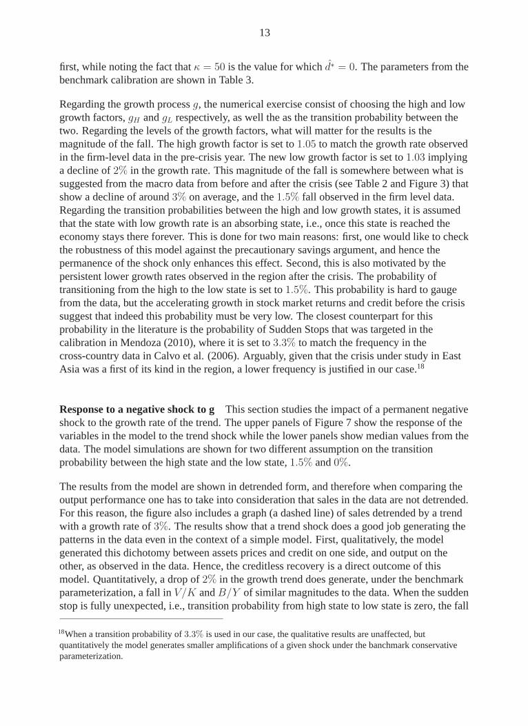
Regarding the growth processg, the numerical exercise consist of choosing the high and lowgrowth factors,gH andgL respectively, as well the as the transition probability between thetwo. Regarding the levels of the growth factors, what will matter for the results is themagnitude of the fall. The high growth factor is set to1.05 to match the growth rate observedin the firm-level data in the pre-crisis year. The new low growth factor is set to1.03 implyinga decline of2% in the growth rate. This magnitude of the fall is somewhere between what issuggested from the macro data from before and after the crisis (see Table 2 and Figure 3) thatshow a decline of around3% on average, and the1.5% fall observed in the firm level data.Regarding the transition probabilities between the high and low growth states, it is assumedthat the state with low growth rate is an absorbing state, i.e., once this state is reached theeconomy stays there forever. This is done for two main reasons: first, one would like to checkthe robustness of this model against the precautionary savings argument, and hence thepermanence of the shock only enhances this effect. Second, this is also motivated by thepersistent lower growth rates observed in the region after the crisis. The probability oftransitioning from the high to the low state is set to1.5%. This probability is hard to gaugefrom the data, but the accelerating growth in stock market returns and credit before the crisissuggest that indeed this probability must be very low. The closest counterpart for thisprobability in the literature is the probability of Sudden Stops that was targeted in thecalibration in Mendoza (2010), where it is set to3.3% to match the frequency in thecross-country data in Calvo et al. (2006). Arguably, given that the crisis under study in EastAsia was a first of its kind in the region, a lower frequency is justified in our case.18

Response to a negative shock to gThis section studies the impact of a permanent negativeshock to the growth rate of the trend. The upper panels of Figure 7 show the response of thevariables in the model to the trend shock while the lower panels show median values from thedata. The model simulations are shown for two different assumption on the transitionprobability between the high state and the low state,1.5% and0%.

The results from the model are shown in detrended form, and therefore when comparing theoutput performance one has to take into consideration that sales in the data are not detrended.For this reason, the figure also includes a graph (a dashed line) of sales detrended by a trendwith a growth rate of3%. The results show that a trend shock does a good job generating thepatterns in the data even in the context of a simple model. First, qualitatively, the modelgenerated this dichotomy between assets prices and credit on one side, and output on theother, as observed in the data. Hence, the creditless recovery is a direct outcome of thismodel. Quantitatively, a drop of2% in the growth trend does generate, under the benchmarkparameterization, a fall inV/K andB/Y of similar magnitudes to the data. When the suddenstop is fully unexpected, i.e., transition probability from high state to low state is zero, the fall

18When a transition probability of3.3% is used in our case, the qualitative results are unaffected, butquantitatively the model generates smaller amplifications of a given shock under the banchmark conservativeparameterization.

14

in all variables is larger. This is because when agents internalize the possibility of a suddenstop, the market value of firms adjust downward at the pre-crisis steady state and fall by lessat the news of the new growth state. Note that under the current and similar parametrizations,the borrowing constraint is always binding, even when agents expect a sudden stop with aprobability as high as3%. In this model, due to the form of the borrowing constraint(becoming tighter the higher the expectation of a negative shock) and the mere possibility ofdebt-equity substitution, firms find it optimal to borrow to the limit as long asβ < 1 + r.

The fall in output generated by the model is smaller than what is observed in the data.However, conservative values have been used for both the leverage andκ, and the effect ofvarying these assumptions would be discussed shortly.

Discussion The simulations suggest that a simple model that incorporates trend shocks canpotentially explain some of the main stylized facts of sudden stops. Some of the patterns inthe data, in particular, the dichotomy between output on one hand and debt levels on theother, cannot be accounted for in a standard business cycle model with TFP shocks. Morespecifically, only very persistent TFP shocks can generate this quasi-permanent downwardadjustment in asset prices, yet such shocks would be inconsistent with a fast recovery inoutput. The model at hand is tractable and its dynamics are simple. Following a permanentdrop in the growth rate, the detrended market value is abruptly and permanently adjusteddownward. Due to binding borrowing constraints, this will also lead to a drop in debt levels.That is, firms would have to adjust their debt levels in one period to satisfy the new andtighter borrowing constraint. To do so, they could decrease their investment (or evendisinvest) and/or they could decrease their payouts (or even issue new equity). If equityissuance did not involve direct costs it would be optimal for firms to maintain their capitallevels which is what happens ifκ = 0. However, withκ > 0, firms will decrease capital andequity payouts in a way to equalize their respective marginal costs. Once debt levels areadjusted firms will rebuild capital over time to reach the pre-crisis steady state as shown inthe upper right panel. Following the recovery of output to its new trend, credit andinvestment are permanently lower due to the lower growth rate.The assumption onβ(1 + r) being smaller than one is a convenient simplification, albeit, nota necessary one. In fact, it is easy to see that large drops in the market value can lead to dropsin borrowing levels even when borrowing constraints are not binding as long as firmsborrowing is beyond a certain level. Second, one could instead assume that the shock takesplace at a non-steady state, a point at which firms are still building up their capital stock andare therefore more likely to have their borrowing constraint binding. Third, one could stillforgo this assumption by incorporating exogenous exit rates, particularly ones whereentrepreneurs get to consume the remaining equity in the firm when they exit. However, suchmodifications would only make the numerical solution (particularly with heterogeneousfirms) more challenging without additional insight.

Financial frictions and leverage Just as in most sudden stops models, financial frictionsare central in generating drops in output in the model. They are captured at the equity payoutlevel in this setting. These frictions are meant to formalize costly adjustment in financing and

15

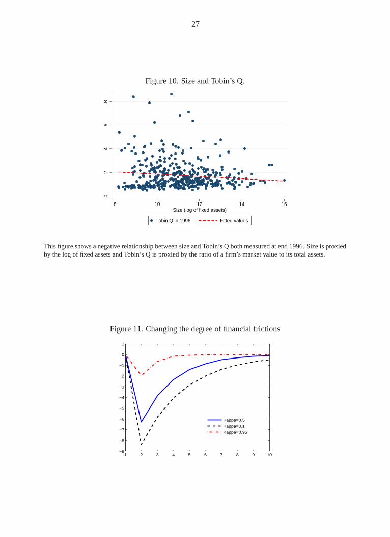
reflect more than just the cost of issuance as explained earlier. The parameterκ whichdetermines the degree of frictions was set to a conservative value as explained earlier. Figure11 shows the impact of the same shock discussed earlier for varying levels ofκ. The resultsshow a stronger impact on output for higher levels ofκ.In this model, output drops occur solely due to financial frictions, triggered by the need todecrease debt levels. The leverage effect is therefore very strong and, as shown in Figure 8,lower values of leverage significantly reduce the impact of the shock on output.

B. Heterogeneous Firms and The Size Effect

Section 2 showed strong evidence of a size effect in that larger firms outperformed the smallerones during the crisis episode in Indonesia, Malaysia and Thailand. Table 1 for examplesuggests that on average a twice larger firm had around5% higher growth rate in salesbetween 1996 and 1998. This difference in performance is large and statistically significant.Furthermore, smaller firms had not only a worse performance in terms of sales but also theirmarket value and their debt collapsed significantlty more than the larger firms. This sectionshows how the model can explain this significant heterogeneity in performance that is due tosize differences. The argument relies on small firms having a higher potential for growth.There is a strong evidence from a large body of empirical research that, on average, smallfirms tend to grow faster than the larger ones (see for example Hall, 1988; Evans, 1987).

The model introduces heterogeneity along the size dimension, as discussed earlier, byallowing firms with decreasing returns production technology to receive shocks to theirtechnology level. It is assumed, for the sake of simplicity, that this technology level can onlytake two valuesaS andaL, with aS < aL. Therefore, at the conditional steady state, firmswith the lower technologyaS are the small firms. Note that the conditional steady state refersto the state at which, ifa′j = aj, thenx′ = x, wherex is any detrended variable in the model.Another simplifying assumption that is made in this section is that the Markov transitionmatrix,Π, is symmetric. This assumption does not involve a loss of generality. In fact, theresults shown here will have the same qualitative properties as long as either ofΠ(S/L) orΠ(L/S) is positive. This implication, nevertheless, helps in pinning down parameters at thecalibration stage. Forη0 = 1/2, i.e., when the shares of small and large firms in the totalsample are equal at time 0,ηt = 1/2 at any timet.

Amplification due to the growth option: A simple example Before showing thequantitative properties of the model with heterogeneous firms, a simple example can give themain intuition behind the result. It is clear to see, that in the model at hand, a larger drop inthe market value implies a larger drop in output, everything else equal. Therefore, a theorybehind the larger volatility in the market value of small firms, alone, can explain the findingsin the data. This property follows directly from the assumption that these firms can grow tobecome large. To simplify the analysis, it is helpful to abstract from the main aspects of themodel and assume that there are large firms and small firms in the economy, that distribute, attime t, dividendsdLΓt anddSΓt respectively, wheredL > dS. Γt is the stochastic trend thatdrives growth in the economy and has the same properties described above. At the beginning

16

of each period small firms can either remain small or become large with a probabilityp.Large firms remain large forever. Under this last assumption the market value of large firmsis significantly simplified and can now be written as:

V L =∞∑

j=0

(βg)jdL (9)

The market value of the small firms is a function ofV L:

V S = dS + βg[pV S + (1− p)V L] (10)

Proposition 2. An unexpected permanent change in the trend’s growth rate has a largerimpact on the value of small firms, in that the absolute value of the percentage change in themarket value of small firms is higher than the one for the large firms.

Proof. It is straightforward to see that bothV S andV L are both strictly increasing ing.Therefore it is enough to show thatV S

V L is strictly increasing ing to prove that the percentagechange inV S is higher in absolute value than the percentage change inV L. Note thatV L = dL

1−βgand therefore:

V S

V L=

dS

dL[1− βg]

1− βg(1− p)+

βgp

1− βg(1− p)

Which can be re-written as:

V S

V L=

dS

dL

1− βg(1− p)[dS

dL−p

dS

dL(1−p)

]

1− βg(1− p)(11)

From this equation it is clear thatVS

V L is strictly increasing ing as long asdS

dL< 1 which is

always true by assumption.19 Q.E.D.

The intuition behind this result is simple. Compared to large firms, a sizable share of thesmall firms’ market value is due to the expectations that the market place on future growthrates. Therefore changes in these expectations will have a larger impact on the market valueof the small firms. In other words, small firms have a “growth option” which itself is afunction of the future growth rates. That is unlike large firms, a fraction of the market valueof the small firms reflects their future opportunities which have not realized yet. Howeverthese opportunities are very sensitive to changes in the growth rates which makes the marketvalue of the small firms relatively more affected by these changes. Note that we haveassumed that the large firms do not become smaller for simplicity. If this was possible, thenthe main logic would still apply. This is because such possibility would only decrease thevolatility of the large firms. Since in the original model the borrowing constraint binds at the

19This follows from the fact that1−xα

1−xis increasing in x ifα < 1.

17

steady state, a larger change in the market value would induce a larger change in the debtlevel of a company. This directly implies that the small firms’ production will also be moreaffected by changes in growth rate. In the following we compare the response of small firmsand large firms to a trend shock in the original model.

Quantitative properties Parameters are chosen such that small and large firms in themodel be representative of the lower and upper third in the sample (ranked by size) (seeFigure 5). The firm-specific productivity parameter of larger firms,aL, is normalized to one.Then,aS is chosen such that the larger firm has three times more capital than the smaller firm.In the data, the smallest of the large firms’ group has three times more capital than the largestof the small firms’ subsample. That is, the size ratio chosen here is conservative.20 The othercentral parameter that needs to be set is the probability of switching size, i.e., the probabilityof smaller firms becoming large and the probability of large firms becoming small. Thisparameter will determine the Tobin’s Q of both the large and the small firms. For this, theprobabilityp is set to match the ratio, in the data in 1996, of the Tobin’s Q of the small firm tothat of the large firms. This ratio is equal to 1.25. Note that given this heterogeneity, evenwhen these firms are subject to the same degree of borrowing constraint they mightaccumulate different ratios of debt to capital. In particular, the fact that the small firm is agrowth firm will allow it to carry more leverage for a given level of financial constraints, dueto its higher ratio of market value to capital. However, since in the data the leverage of bothlarge firms and small firms are not significantly different, the parametersφS andφL arechosen in way to set tighter constraint on the small firms to generate the same leverage ratiothat is in the data which is around 0.52. This is done to separate the size from the leverageeffect; indeed, if small firms were allowed to have a higher leverage this will further amplifythe results. Finally, note that although a small firm can acquire a new technology overnight,due to the borrowing constraint it might not be able to accumulate the optimal capital in oneperiod. That is, unlike the earlier simple example, in this case small firms have to follow apath to become large firms which starts at the period in which they acquire the newtechnology. The results are shown in Figure 9. The parameters’ values are shown in Table 4.Note that for simplicity, we assume the trend shock in this exercise to be unanticipated.

The upper panel in the figure shows that both the the market value of the large and the smallfirm decrease following a1.5% permanent negative shock to the growth rate, but that the dropin the market value of small firms is significantly larger. This is where the size effect comesin play. Its impact on the other variables, notably the output, is only due to the difference inthe market value’s reaction to the shock. The lower panel shows the reaction of the output.The detrended output of the small firm drops significantly more, before it recovers relativelyquickly to the pre-crisis level. Based on the assumptions in this paper alone, only trendshocks, as opposed to TFP level shocks, can generate this size effect. This is because, unlikethe growth shock, a TFP shock affects directly the firm’s output and subsequent changes inthe market value are led by the output drop. The story proposed by the model is one based onthe assumption that small firms are growth firms, and one where the amplification

20Since the model is solved in a non linear way through iterations over the grid, keeping the size difference to aminimum significantly shortens the computational time.

18

mechanisms of firms’ leverage play a central role. Were small firms to be significantly lessleveraged, the leverage effect would have likley compensated the size effect; however, thedata do not suggest a lower leverage for small firms. When heterogeneity is added to themodel, it allows for various effects that could stem from differences in borrowing decisionsbetween small and large firms. In fact, the condition thatβ(1 + r) < 1 is no longer sufficientfor firms to borrow to the limit as in the case with homogeneous firms. For example, forsignificantly higher values of p, small firms see a benefit of not borrowing to limit, so whenthe likely switch to a higher level takes place, they are able to finance the necessary increasein capital to reach the new optimal level in a minimal time. However, such values of p wouldgenerate much larger differences in Tobin’s Q compared to what is observed in the data. Asfor the larger firms, they will borrow to the limit, for a even larger range of probabilities. Thisis because their switch to a lower size involves selling of existing capital, which is optimalunder their new technology levels, hence they have no motives for precautionary action.

The growth effect: back to the data The model suggests that the underperformance ofsmall firms is related to their growth option. This characteristic of small firms results in amore responsive market value to changes in trend growth. Larger adjustments in a firm’svalue consequently lead to a larger drop in output. Testing the validity of this channel in thedata, however, is challenging for two main reasons. First, the data do not provide a direct orunequivocal measure of growth opportunities. While Tobin’s Q might be the best availablemeasure, and a variable that has a direct counterpart in the model, it is often correlated withcurrent firms’ performance and other information related to its current investment levels.Second, assuming that a direct measure of growth opportunities is available, the model onlypredicts that its positive relationship with future performance will be weakened; whetherhigher growth opportunities will lead to lower performance overall depends on theimportance of the negative trend shock.21 With this in mind, a proxy of Tobin’s Q (the ratioof market value to total assets in 1996,V/K) is introduced as an explanatory variable in thesame regressions shown in Section 2. Table 5 shows the results from these regressions. Thefirst two columns in the table recapitulate the results from earlier regressions in section 2.The third and fourth columns introduceQ as an explanatory to the same regression. In theregressions with the change in sales as the dependent variable, in column 3, introducingQ tothe earlier regressions leads to a negative and significant coefficient. However, the size effectremains positive and significant, although its coefficient decreases in magnitude by around15% with the introduction ofQ, and its now only significant at the10%. In the fouth column,where the dependent variable is the change in value, the introduction ofQ leads to a negativecoefficient yet not significant. The coefficient on size also decerases by around11%, butremains significant. In the fifth and sixth columns, the size is excluded and replaced byQ.This leads to negative and significant coefficients in both regerssions. Overall, the resultsfrom these regressions are supportive of the model’s prediction. Both measures ofperformance reflect, to a degree, a “growth effect”, but the size effect is still significantlypresent in the regressions where the change in sales is the endogeneous variable. Whetherthis is due to the problems with measuring growth opportunities as discussed earlier, or to

21In each period in the model a fraction of small firms receive a new and better technology. This creates apositive relationship between growth opportunities and next period’s performance in a non-crisis environment.

19

other effects that are not controlled for in the regression (e.g. ownership, relationship withbanks, or corporate governance) is something that is hard to gauge with the limited availabledata. Nevertheless, the mere finding of a negative relationship between growth opportunitiesand performance during the crisis is surprising given that higher Tobin’s Q is a predictor ofgood performance. This new finding documented in this paper, is predicted by the modelwhen trend shocks are the main driving force behind the collapse in firms’ market value.

IV. C ONCLUDING REMARKS

This paper studied firms’ recovery from a Sudden Stop in a sample of publicly listed firms inSoutheast Asia. The data show an unambiguous dichotomy between the behavior of sales,which recover relatively swiftly, and that of Tobin’s Q, debt levels, and investment whichshow a persistent collapse and remain well below their pre-crisis levels. Although thesepatterns were shared by most firms in the sample, the data show significant heterogeneity,notably between firms of different size and different pre-crisis leverage. The paperformulates a model that can account for these patterns. The model has two main novelfeatures. First it incorporate trend shocks in a model with financial frictions in the form of anendogenous borrowing constraint and a constraint on equity issuance. These shocks aremotivated by the persistent decline in post-crisis growth rates in the data, as well as thequasi-permanent collapse in asset prices. Standard TFP shocks cannot generate such patterns.Once trend shocks are taken into account, the model shows that they can rationalize the mainobservations from both the aggregate as well as the firm-level data. The simulations showhow a permanent decline in trend productivity, reduce permanently the market value andconsequently the debt level of firms. Nevertheless, output recovers to its pre-crisis optimallevel (in de-trended terms) after a short-lived yet large drop, which is due to financialfrictions. Firms’ leverage play a central role in generating output drops. In the data, firmswith very low leverage barely show any reduction in their output despite the large drop intheir market value. The model generates a similar pattern since the drop in the market valueis due to the trend shock, but the transmission of the shock to output hinges on a sizableleverage, even when borrowing constraints are binding. Another novelty in the paper is themodeling of firms of different size which is based on the assumption that small firms aregrowth firms, to which there is support in the data as well as in the literature. Thisassumption alone will lead to a larger response to trend shocks from small firms’ marketvalue. The data show that Tobin’s Q and size are correlated and that the first capture some ofthe size effect that is seen in the regressions, despite the fact that Tobins’ Q is usuallystrongly and positively associated with an increase in future sales.

One major shortcoming of this paper is that it models trend shocks as an exogenous factor,and remains silent about the factors that could lead to this sudden downward shift in thetrend. Despite the recent literature on the role of these shocks in emerging markets’ businesscycle, they remain largely unexplained and therefore an avenue for future research. Theresults in this paper also call for further research into whether a combination of trend shocksand financial frictions could improve the explanatory powers of Sudden Stop models.

20

V. APPENDIX

A. Solution

First order conditions Let λ andµ be the Lagrange multipliers on the budget constraintand the borrowing constraint respectively. Taking the derivatives we get:

d : 1− λϕd(d) = 0 (12)

b′ : −µφ+λ

1 + r+ (β + µ)EVb′(k

′, b′, a′, g′) = 0 (13)

k′ : (β + µ)EVk′(k′, b′, a′, g′)− µ = 0 (14)

(15)

The envelope conditions are:

Vk(k, b, a, g) = λ(fk(k, b, a, g) + (1− δ)) (16)

Vb(k, b, a, g) = −λ (17)

(18)

Numerical Procedure The numerical procedure solves the model nonlinearly to allow forthe possibility that the borrowing constraint does not bind under certain parameterizationsand during the transition following the shock. The approach consists of approximating theconditional expectations in (13) and (14) and in the objective function as functions of thestate variables through a finite element representation that interpolates linearly between thegrid points of the state space. For the case of homogeneous firms, we first solve for the steadystates for each value ofg and set accordingly the space of the grids. We then make a guessabout the value function and its derivatives with respect to the state variables. For theseguesses one can solve for all the variables assuming the borrowing constraint binds. Ifµ, theLagrange multiplier on the borrowing constraint, is positive, this means the borrowingconstraint is indeed binding. Otherwise, we solve the problem again settingµ = 0 since thismeans that the constraint does not bind. This is done at every grid. The grid points are joinedwith bilinear functions so that the approximate functions are continuous. We update theinitial guesses until convergence. Note that the problem with heterogeneous firms is solved ina similar way, however the steady state values are computing simultaneously during iterationprocedure taking the homogeneous steady state results for each firm’s parametrization as aninitial guess.

21

B. Figures and Tables

Figure 1. The ratio of credit to GDP.

050

100

150

200

1990 1995 2000 2005 2010

Indonesia Malaysia Thailand

Data source: World Development Indicators, World Bank.

Figure 2. MSCI market indices

020

040

060

080

0

1990 1995 2000 2005 2010

Indonesia Malaysia Thailand

22

Figure 3. Real GDP and its growth rate.

1991 1998 200680

100

120

140Indonesia − RGDP

1991 1998 2006

−0.1

−0.05

0

0.05

0.1Indonesia − growth rates

1991 1998 200660

80

100

120

140Thailand − RGDP

1991 1998 2006

−0.1

−0.05

0

0.05

0.1Thailand − growth rates

1991 1998 200650

100

150Malaysia − RGDP

1991 1998 2006−0.1

−0.05

0

0.05

0.1

Malaysia − growth rates

The left panels in this figure plot an index of the real GDP in Indonesia, Malaysia and Thailand between 1991 and2006. The right panels plot the growth rates in the real GDP during this period. The three countries experiencedtheir largest losses in output in the year 1998. Data source: IFS.

23

Figure 4. Indices of firms’ average sales, debt, investment and market value.

1996 1998 2000 2002 200490

95

100

105

110

115

1996 1998 2000 2002 200470

80

90

100

110

120

1996 1998 2000 2002 200420

40

60

80

100

120

1996 1998 2000 2002 200440

60

80

100

120

Sales DebtSales

Invest.Sales

Value*Sales

Notes: * Except forValuewhich is a beginning-of-year index since it precedes the drop in other variables, otherindices are end-of-year values. Data source: Worldscope, Thomson Financial.

24

Figure 5. Comparing the performance of large and small firms.

1996 1998 2000 2002 200480

90

100

110

120Sales

1996 1998 2000 2002 200450

60

70

80

90

100Debt

1996 1998 2000 2002 200420

40

60

80

100Investment

1996 1998 2000 2002 200420

40

60

80

100Market Value

LargeSmall

Notes: Figure 5 plots an index of average sales, debt, investment and credit where the 1997 value is normalizedto 100. The dotted line shows the figure for the larger companies while the solid line is for the smaller firms.Firms are ranked by their size in 1996 based on the dollar value of their fixed assets (upper and lower terciles).Data source: Worldscope, Thomson Financial.

Figure 6. The impact of the crisis on low leverage firms.

1996 1998 2000 2002 200490

100

110

120

130

140Sales

1996 1998 2000 2002 200440

50

60

70

80

90

100Market Value

1997 1998 1999 2000100

120

140

160

180

200

220Profit of small buis.

Notes: The left and center panel contrast the performance of low-leverage firms (dashed line), defined as firmswith a leverage below the 10th centile which corresponds to 0.2, and that of the average firm in the sample. Thepanel on the right shows the median profits for household businesses in Thailand during the crisis (see Paulsonand Townsend (2005) for a more detailed description of the sample).

25

Figure 7. The benchmark parametrization

0 10 20 30 40−60

−50

−40

−30

−20

−10

0

%

Model: V/K

0 10 20 30 40−60

−50

−40

−30

−20

−10

0Model: B/Y

0 5 10 15 20−7

−6

−5

−4

−3

−2

−1

0Model: Y

0 2 4 6 8−70

−60

−50

−40

−30

−20

−10

0

%

Data: V/K

0 2 4 6 8−40

−30

−20

−10

0

10Data: B/Y

0 2 4 6 8−15

−10

−5

0

5

10

15Data: Y

p=0p=1.5%

DataDe−trended

26

Figure 8. The leverage effect

0 1 2 3 4 5 6 7 8 9−60

−40

−20

0

1 2 3 4 5 6 7 8 9 10−8

−6

−4

−2

0

B/K=0.5B/K=0.25B/K=0.1

Figure 9. The size effect

0 1 2 3 4 5 6 7 8 9 10−0.7

−0.6

−0.5

−0.4

−0.3

−0.2

−0.1

0Market Value

1 2 3 4 5 6 7 8 9 10−0.08

−0.07

−0.06

−0.05

−0.04

−0.03

−0.02

−0.01

0Output

SmallLarge

27

Figure 10. Size and Tobin’s Q.

02

46

8

8 10 12 14 16Size (log of fixed assets)

Tobin Q in 1996 Fitted values

This figure shows a negative relationship between size and Tobin’s Q both measured at end 1996. Size is proxiedby the log of fixed assets and Tobin’s Q is proxied by the ratio of a firm’s market value to its total assets.

Figure 11. Changing the degree of financial frictions

1 2 3 4 5 6 7 8 9 10−9

−8

−7

−6

−5

−4

−3

−2

−1

0

1

Kappa=0.5

Kappa=0.1

Kappa=0.95

28

Table 1. Determinants of firms’ performance during the crisis.

Notes: The sample is formed by merging data from Indonesia, Malaysia and Thailand after converting all valuesto the U.S. dollar of 2000. The dependent variables are the changes in the log of sales and market value betweenend-1996 and end-1998. The last four columns exclude the non-tradable (NT) sector and the tradable (T) sector,respectively. The table shows the output of simple OLS regressions. The explanatory variables are from end-1996.Sizeis a measure of firms’ fixed assets.Export is a dummy that takes the value one for exporters.Leverageis the ratio of total liabilities to total assets.Interestis the ratio of the total interest payments to total liabilities.Profitability is the ratio of net income to total assets.Dividendsis a dummy that takes the value one for firmsthat paid dividends in 1996.Investmentis the ratio of investment to total assets on end-1996. The regressionalso includes a dummy for Thailand, a dummy for Indonesia and dummies based on the SIC codes to capture theindustry effects. Data source: Worldscope, Thomson Financial.

(1) (2) (3) (4) (5) (6)∆ Sales ∆ Value ∆ Sales ∆ Value ∆ Sales ∆ Value

Size 0.0468** 0.0760** 0.0697*** 0.113*** 0.0483** 0.0183(2.15) (2.46) (3.06) (2.90) (2.49) (0.48)

Export 0.193*** 0.222** 0.129** 0.102(2.93) (2.38) (2.18) (0.89)

Leverage -0.309* -0.818*** -0.339* -1.096*** 0.110 -0.604*(-1.82) (-3.39) (-1.90) (-3.49) (0.68) (-1.92)

Profit. 0.583* 0.603 -0.900* 2.192*** -0.767** 0.820(1.78) (1.30) (-1.94) (2.68) (-2.09) (1.59)

Interest -0.431 -1.128 -1.510 1.002 -2.389** -3.956*(-0.37) (-0.69) (-1.28) (0.49) (-1.99) (-1.72)

Dividends -0.109 0.0179 -0.0543 0.0127 0.0859 0.213(-1.13) (0.13) (-0.52) (0.07) (0.90) (1.08)

W. Capital -0.215 -0.172 -0.387** -0.745** -0.00257 -0.655*(-1.19) (-0.66) (-2.18) (-2.39) (-0.01) (-1.94)

Investment 0.659** -1.002** 0.856** -1.079* -0.0400 -0.899(2.09) (-2.26) (2.59) (-1.90) (-0.12) (-1.45)

Thailand -0.107 0.254** 0.00795 0.317** 0.00969 0.458***(-1.37) (2.28) (0.10) (2.31) (0.13) (3.25)

Indonesia 0.0182 0.0470 -0.0406 -0.114 0.205** 0.0639(0.17) (0.31) (-0.43) (-0.70) (2.44) (0.38)

Indust. YES YES YES YES YES YES

Constant -0.455* -1.629*** -0.570* -2.101*** -0.609** -1.236**(-1.68) (-4.24) (-1.97) (-4.20) (-2.48) (-2.57)

R2 0.186 0.206 0.164 0.208 0.164 0.150

t statistics in parentheses* p<0.10, ** p<0.05, *** p<0.01

29

Table 2. Average growth rates before and after the crisis.

Notes: The data are taken from the IFS. The table shows the simple average of growth rates before and after the

crisis. The standard errors are shown in italic. A t-test rejects the equality of the means between the two samples.

Indonesia Malaysia ThailandAnnual:1985− 1996 0.068 0.084 0.092

Standard errors 0.009 0.027 0.023Annual:1990− 1996 0.072 0.095 0.086

Standard errors 0.006 0.004 0.015Annual:2000− 2006 0.049 0.055 0.051

Standard errors 0.0067 0.025 0.015Annual:2000− 2008 0.052 0.055 0.048

Standard errors 0.008 0.022 0.015

Table 3. Benchmark Calibration

Description Parameter ValuesDiscount factor β = 0.94Growth factor g = 1.05Interest rate r = 0.041Depreciation rate δ = 0.062Share of capital α = 0.71Borrowing constraint parameter φ = 9.85Cost of equities parameter κ = 0.5

Table 4. Calibration for the small and the large firms.

Description Parameter ValuesDiscount factor β = 0.94Growth factor g = 1.05Interest rate r = 0.041Depreciation rate δ = 0.062Share of capital α = 0.71Borrowing constraint parameter φL = 7.9 φS = 12.4Probability of switching p = 0.021Cost of equities parameter κ = 0.5

30

Table 5. The “growth effect’.

Notes: The dependent variables are: the change in the log of sales between end-1996 and end 1998, and thechange in the log of the market value over the same period.Q is the ratio of the market value of a firm to its totalassets at end-1996, which is direct counterpart of the model’s Tobin’s Q. It is a proxy, for the market value of thegrowth opportunities of a firm. Data source: Worldscope, Thomson Financial.

(1) (2) (3) (4) (5) (6)∆ Sales ∆ Value ∆ Sales ∆ Value ∆ Sales ∆ Value

Size 0.0468** 0.0760** 0.0395* 0.0671**(2.15) (2.46) (1.71) (2.12)

Export 0.193*** 0.222** 0.170** 0.207** 0.180*** 0.225**(2.93) (2.38) (2.48) (2.21) (2.63) (2.39)

Leverage -0.309* -0.818*** -0.353** -0.825*** -0.346* -0.813***(-1.82) (-3.39) (-2.01) (-3.42) (-1.97) (-3.35)

Profit. 0.583* 0.603 0.709** 0.746 0.741** 0.796*(1.78) (1.30) (2.05) (1.57) (2.14) (1.67)

Interest -0.431 -1.128 -0.384 -1.317 -0.478 -1.511(-0.37) (-0.69) (-0.32) (-0.80) (-0.40) (-0.92)

Dividends -0.109 0.0179 -0.103 0.00338 -0.0835 0.0331(-1.13) (0.13) (-0.98) (0.02) (-0.80) (0.23)

W. Capital -0.215 -0.172 -0.248 -0.160 -0.299 -0.246(-1.19) (-0.66) (-1.32) (-0.62) (-1.60) (-0.96)

Investment 0.659** -1.002** 0.691** -0.938** 0.757** -0.820*(2.09) (-2.26) (2.13) (-2.11) (2.34) (-1.85)

Thailand -0.107 0.254** -0.157* 0.218* -0.171** 0.197*(-1.37) (2.28) (-1.88) (1.91) (-2.04) (1.72)

Indonesia 0.0182 0.0470 0.00850 0.0320 0.00687 0.0279(0.17) (0.31) (0.08) (0.21) (0.06) (0.18)

Indust. YES YES YES YES YES YES

Q -0.0317* -0.0331 -0.0381** -0.0441*(-1.76) (-1.34) (-2.16) (-1.82)

Constant -0.455* -1.629*** -0.294 -1.445*** 0.139 -0.705***(-1.68) (-4.24) (-0.99) (-3.55) (0.89) (-3.32)

R2 0.186 0.206 0.192 0.210 0.184 0.199

t statistics in parentheses* p<0.10, ** p<0.05, *** p<0.01

31

References

Adam, C. and D. Bevan, 2006, “Aid and the Supply Side: Public Investment, Export Performance, and Dutch Disease in Low-Income Countries,” The World Bank Economic Review, Vol. 20, No. 2, pp. 261–290.

Aghion, P., P. Bacchetta, and A. Banerjee, 2004, “Corporate balance-sheet approach to

currency crises, ” Journal of Economic Theory, Vol. 119, Issue 1, pp. 6-30. Aguiar, M., and F.A. Broner, 2006, “Determining underlying macroeconomic fundamentals during emerging market crises: Are conditions as bad as they seem? ” Journal of

Monetary Economics, Volume 53, Issue 4, pp. 699-724. _____, and G. Gopinath, 2006, “Defaultable debt, interest rates and the current account.” Journal of International Economics, Vol. 69, No. 1, pp. 64-83. _____, 2007, “Emerging Market Business Cycles: The Cycle is the Trend. ” Journal of

Political Economy, Vol. 115, No. 1, pp. 69-102. Allen, F., A. Bernardo, and I. Welch, 2000, “A Theory of Dividends Based on Tax

Clienteles.” Journal of Finance, Vol. 55, pp. 2499-2536. Barro, R., 2001, “Economic Growth in East Asia Before and After the Financial Crisis.”

NBER Working Paper, No. 8330. Bernanke, B., M. Gertler, M., and S. Gilchrist, 1999, “The Financial Accelerator in a

Quantitative Business Cycle Framework. ” Handbook of Macroeconomics, Volume 1C, chapter 21, Amsterdam: Elsevier Science.

Borensztein, E., and J.W. Lee, 2002, “Financial crisis and credit crunch in Korea: evidence

from firm-level data. ” Journal of Monetary Economics, Volume 49, Issue 4, pp. 853-875.

Braggion, F., L. Christiano, and J. Roldos, 2009, “Optimal Monetary Policy in a Sudden

Stop.” Journal of Monetary Economics, Volume 56, Issue 4, pp. 582-595. Caballero, R., and A. Krishnamurthy, 2001, “International and domestic collateral constraints

in a model of emerging market crises. ” Journal of Monetary Economics, Volume 48, Issue 3, pp. 513-548.

Calvo, G.A., 1998, “Capital Flows and Capital-Market Crises: The Simple Economics of

Sudden Stops. ” Journal of Applied Economics, Vol. 1, pp. 35-54.

32

_____, A. Izquierdo, and E. Talvi, 2006, “Sudden Stops and Phoenix Miracles in

Emerging Markets. ” American Economic Review, Papers and Proceedings, Vol. 96, No. 2.

Cerra, V., and S. Saxena, 2008, “Growth Dynamics: The Myth of Economic Recovery. ”

American Economic Review, Volume 98, Issue: 1, pp. 439-457. Chari, V.V., P. Kehoe, and E. McGratten, 2005, “Sudden Stops and Output Drops.” Federal Reserve Bank of Minneapolis, Staff Report no. 353. Chang, R., and A. Fernandez, 2009, “On the sources of aggregate fluctuations in emerging

economies. Mimeo. Claessens, S., S. Djankov, and L.C. Xu, 2000, “Corporate performance in the East

Asian financial crisis. ” The World Bank Research Observer. Cooper, R., and Ejarque, 2003, “Financial Frictions and Investment: Requiem in Q.”

Review of Economic Dynamics, 6, pp. 710-728. Evans, D., 1987, “The Relationship Between Firm Growth, Size, and Age: Estimates for

100 Manufacturing Industries. ” The Journal of Industrial Economics, Vol. 35, pp. 567-581.

Guttman, I., O. Kadan, and E. Kandel, 2006, “A Rational Expectations Theory of Kinks in

Financial Reporting. ” Accounting Review, Vol. 81, pp. 811-848. Hall, B., 1988, “The relationship between firm size and firm growth in the U.S.

manufacturing center. ” NBER Working Paper No. 1965. Hennessy, C. A., and T.M. Whited, 2007, “How Costly is External Financing? Evidence

from a Structural Estimation, ” Journal of Finance, No. 4, pp. 1706-1745. Iannariello, M.P., H. Morsy, and A. Terada-Hagiwara, 2007, “Role of Debt Maturity

Structure on Firm Fixed Assets during Sudden Stop Episodes: Evidence from Thailand,” IMF Working Papers, 07/11.

Jermann, U., and V. Quadrini 2005, “Financial Innovations and Macroeconomic

Volatility.” NBER Working Paper No. 12308. Kim, B., and L. Inmoo, 2003, “Agency problems and performance of Korean companies

33

during the Asian financial crisis: Chaebol vs. non-chaebol firms.” Pacific-Basin Finance Journal, pp. 327-348.

Kim, D., D. Palia, and A. Saunders, 2003, “The Long-Run Behavior of Debt and Equity

Underwriting Spreads. Mimeo, Stern School of Business, NYU. Kiyotaki, N., and J.H. Moore, 1997, “Credit Cycles. ” Journal of Political Economy, Vol.

105(2), pp. 211-48. Krugman, P., 1999, “Balance sheets, the transfer problem, and financial crises.”

International Tax and Public Finance, Volume 6, Number 4. Liberti, K., and A. Mian, 2010, “Collateral spread and financial development.” The

Journal of Finance, Forthcoming. Lintner, J., 1956, “Distribution of Incomes of Corporations Among Dividends, Retained

Earnings, and Taxes. ” American Economic Review, Vol. 46, pp. 97-113. Mendoza, E.G., 2002, “Credit, Prices and Crashes: Business Cycles with a Sudden Stop. In

S. Edwards and J. Frankel, editors, Preventing Currency Crises in Emerging Markets,” NBER Working Paper, No. 8338.

______, and K. Smith, 2005, “Quantitative implications of a debt-deflation theory

of Sudden Stops and Asset Prices.” Journal of International Economics, Vol. 70(1), pp. 82-114.

Mendoza, E.G., 2010, “Sudden Stops, Financial Crises and Leverage.” American Economic

Review, Forthcoming. Miller, H. M., and K. Rock, 1985, “Dividend Policy under Asymmetric Information.” The

Journal of Finance, Vol. 40, pp. 1031-1051. Mitton, T., 2002, “A cross-firm analysis of the impact of corporate governance on the East

Asian financial crisis. ” Journal of Financial Economics, Volume 64, pp. 215-241. Neumeyer, P.A., and F. Perri, 2005, “Business Cycles in Emerging Economies: The Role of

Interest Rates. ” Journal of Monetary Economics, Vol. 52(2), pp. 345-380. Paulson, A., and R. Townsend, 2005, “Financial Constraints and Entrepreneurship:

Evidence from the Thai Financial Crisis. ” Economic Perspectives, Federal Reserve Bank of Chicago, pp. 34-48.

34

Pratap, S., and C. Urrutia 2004, “Firm Dynamics, Investment and Debt Portfolio: Balance Sheet Effects of the Mexican Crisis of 1994.” Journal of Development Economics (Conference Volume), Vol. 75, No. 2, 535-563.

Ranciere, R., Tornell, A., and F. Westermann, 2008, “Systemic Crises and Growth.” The

Quarterly Journal of Economics, pp. 359-406. Simon, H.A., 1960, “Some further notes on a class of skew distribution functions.”

Information and Control, Vol. 2, 80-88. Yue, V., 2010, “Sovereign default and debt renegotiation.” Journal of International

Economics, Volume 80, Issue 2, pp. 176-187.