Embed Size (px)
Citation preview

Productivity and Trade Dynamicsin Sudden Stops
Felipe Benguria Hidehiko Matsumoto Felipe E. Saffie
University of Kentucky GRIPS - Japan University of Virginia
CBC-IDB-JIE Conference
May 2021
Introduction
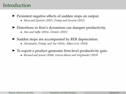
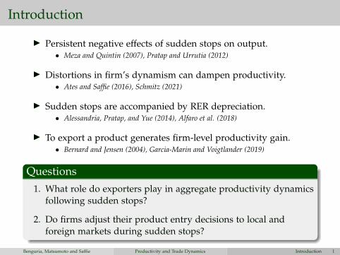
I Persistent negative effects of sudden stops on output.• Meza and Quintin (2007), Pratap and Urrutia (2012)
I Distortions in firm’s dynamism can dampen productivity.• Ates and Saffie (2016), Schmitz (2021)
I Sudden stops are accompanied by RER depreciation.• Alessandria, Pratap, and Yue (2014), Alfaro et al. (2018)
I To export a product generates firm-level productivity gain.• Bernard and Jensen (2004), Garcia-Marin and Voigtlander (2019)
Questions1. What role do exporters play in aggregate productivity dynamics
following sudden stops?
2. Do firms adjust their product entry decisions to local andforeign markets during sudden stops?
Benguria, Matsumoto and Saffie Productivity and Trade Dynamics Introduction 1
Introduction
I Persistent negative effects of sudden stops on output.• Meza and Quintin (2007), Pratap and Urrutia (2012)
I Distortions in firm’s dynamism can dampen productivity.• Ates and Saffie (2016), Schmitz (2021)
I Sudden stops are accompanied by RER depreciation.• Alessandria, Pratap, and Yue (2014), Alfaro et al. (2018)
I To export a product generates firm-level productivity gain.• Bernard and Jensen (2004), Garcia-Marin and Voigtlander (2019)
Questions1. What role do exporters play in aggregate productivity dynamics
following sudden stops?
2. Do firms adjust their product entry decisions to local andforeign markets during sudden stops?
Benguria, Matsumoto and Saffie Productivity and Trade Dynamics Introduction 1
This Paper
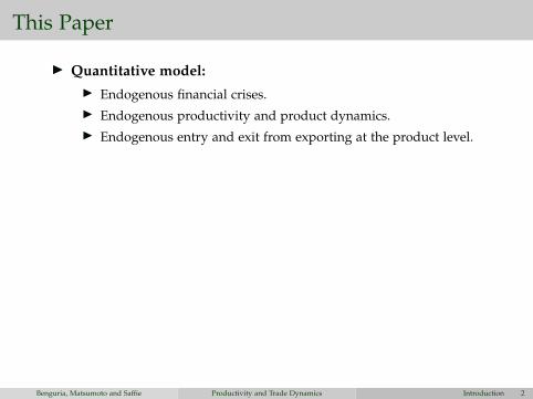
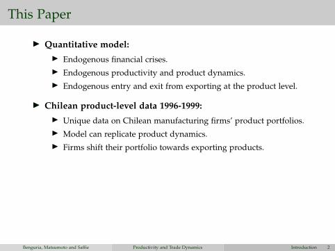
I Quantitative model:I Endogenous financial crises.I Endogenous productivity and product dynamics.I Endogenous entry and exit from exporting at the product level.
I Chilean product-level data 1996-1999:I Unique data on Chilean manufacturing firms’ product portfolios.I Model can replicate product dynamics.I Firms shift their portfolio towards exporting products.
I Main results:I The collapse of domestic product entry drives the short-run
impact of the crisis.I The persistence of the crisis is mostly driven by the product level
exporting dynamics.I 30% of welfare effects are attributed to endogenous firm dynamics.
Benguria, Matsumoto and Saffie Productivity and Trade Dynamics Introduction 2
This Paper
I Quantitative model:I Endogenous financial crises.I Endogenous productivity and product dynamics.I Endogenous entry and exit from exporting at the product level.
I Chilean product-level data 1996-1999:I Unique data on Chilean manufacturing firms’ product portfolios.I Model can replicate product dynamics.I Firms shift their portfolio towards exporting products.
I Main results:I The collapse of domestic product entry drives the short-run
impact of the crisis.I The persistence of the crisis is mostly driven by the product level
exporting dynamics.I 30% of welfare effects are attributed to endogenous firm dynamics.
Benguria, Matsumoto and Saffie Productivity and Trade Dynamics Introduction 2
Literature
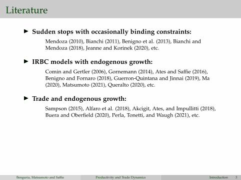
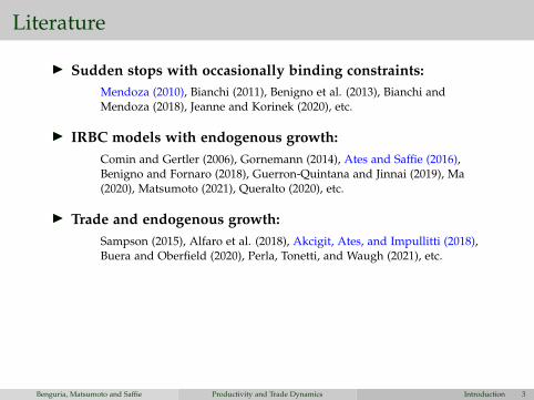
I Sudden stops with occasionally binding constraints:Mendoza (2010), Bianchi (2011), Benigno et al. (2013), Bianchi andMendoza (2018), Jeanne and Korinek (2020), etc.
I IRBC models with endogenous growth:Comin and Gertler (2006), Gornemann (2014), Ates and Saffie (2016),Benigno and Fornaro (2018), Guerron-Quintana and Jinnai (2019), Ma(2020), Matsumoto (2021), Queralto (2020), etc.
I Trade and endogenous growth:Sampson (2015), Alfaro et al. (2018), Akcigit, Ates, and Impullitti (2018),Buera and Oberfield (2020), Perla, Tonetti, and Waugh (2021), etc.
Contributions1. Model: Endogenous crises, firms and trade dynamics.
2. Data: Firm’s product portfolio dynamics during crises andproduct level validation of Klette and Kortum (2004).
Benguria, Matsumoto and Saffie Productivity and Trade Dynamics Introduction 3
Literature
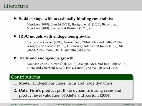
I Sudden stops with occasionally binding constraints:Mendoza (2010), Bianchi (2011), Benigno et al. (2013), Bianchi andMendoza (2018), Jeanne and Korinek (2020), etc.
I IRBC models with endogenous growth:Comin and Gertler (2006), Gornemann (2014), Ates and Saffie (2016),Benigno and Fornaro (2018), Guerron-Quintana and Jinnai (2019), Ma(2020), Matsumoto (2021), Queralto (2020), etc.
I Trade and endogenous growth:Sampson (2015), Alfaro et al. (2018), Akcigit, Ates, and Impullitti (2018),Buera and Oberfield (2020), Perla, Tonetti, and Waugh (2021), etc.
Contributions1. Model: Endogenous crises, firms and trade dynamics.
2. Data: Firm’s product portfolio dynamics during crises andproduct level validation of Klette and Kortum (2004).
Benguria, Matsumoto and Saffie Productivity and Trade Dynamics Introduction 3
Model
Benguria, Matsumoto and Saffie Productivity and Trade Dynamics Model 3
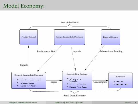
Model Economy:
Foreign Demand Foreign Intermediate Producers Financial Markets
Domestic Intermediate Producers
I Product and Firm Dynamics
I Exporting Margin
I Productivity Growth
Domestic Final Producer
I International
Borrowing
I Collateral Constraint
I Manages Fixed Asset
Household
I Consumes
I Supplies Labor
Rest of the World
Small Open Economy
Exports
Replacement Risk Imports International Lending
Inputs Consumption
Benguria, Matsumoto and Saffie Productivity and Trade Dynamics Model 4
Final Goods Sector: Mendoza (2010)
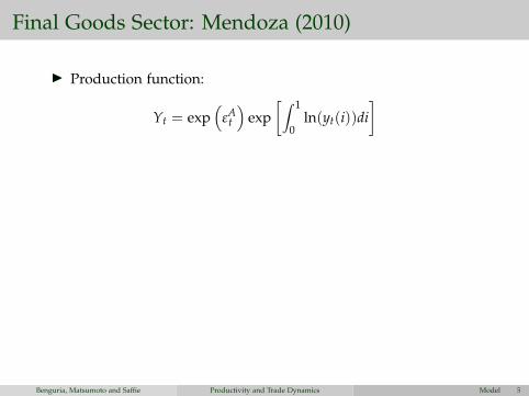
I Production function:
Yt = exp(
εAt
)exp
[∫ 1
0ln(yt(i))di
]
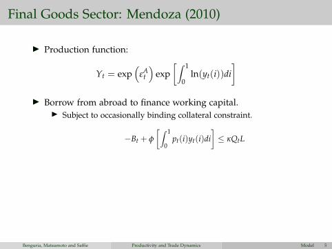
I Borrow from abroad to finance working capital.I Subject to occasionally binding collateral constraint.
−Bt + φ
[∫ 1
0pt(i)yt(i)di
]≤ κQtL
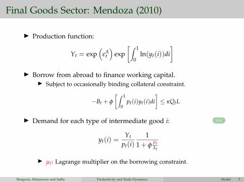
I Demand for each type of intermediate good i: FOC
yt(i) =Yt
pt(i)1
1 + φµtλt
I µt: Lagrange multiplier on the borrowing constraint.
Benguria, Matsumoto and Saffie Productivity and Trade Dynamics Model 5
Final Goods Sector: Mendoza (2010)
I Production function:
Yt = exp(
εAt
)exp
[∫ 1
0ln(yt(i))di
]I Borrow from abroad to finance working capital.
I Subject to occasionally binding collateral constraint.
−Bt + φ
[∫ 1
0pt(i)yt(i)di
]≤ κQtL
I Demand for each type of intermediate good i: FOC
yt(i) =Yt
pt(i)1
1 + φµtλt
I µt: Lagrange multiplier on the borrowing constraint.
Benguria, Matsumoto and Saffie Productivity and Trade Dynamics Model 5
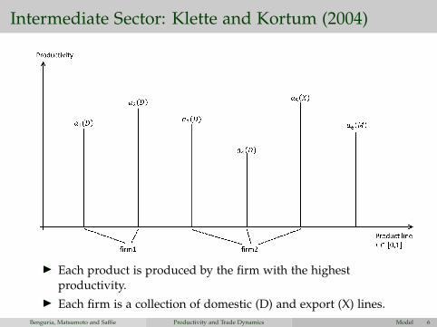
Intermediate Sector: Klette and Kortum (2004)
I Each product is produced by the firm with the highestproductivity.
I Each firm is a collection of domestic (D) and export (X) lines.Benguria, Matsumoto and Saffie Productivity and Trade Dynamics Model 6
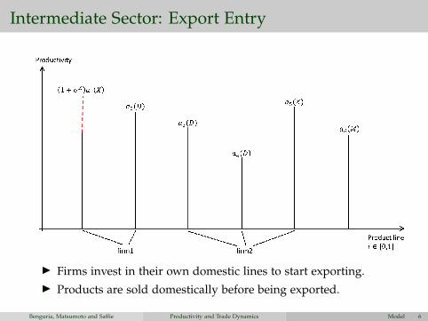
Intermediate Sector: Export Entry
I Firms invest in their own domestic lines to start exporting.I Products are sold domestically before being exported.
Benguria, Matsumoto and Saffie Productivity and Trade Dynamics Model 6
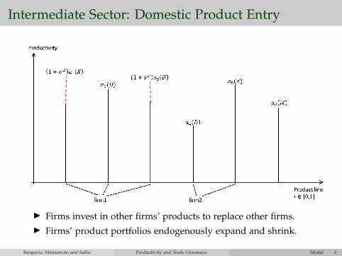
Intermediate Sector: Domestic Product Entry
I Firms invest in other firms’ products to replace other firms.I Firms’ product portfolios endogenously expand and shrink.
Benguria, Matsumoto and Saffie Productivity and Trade Dynamics Model 6
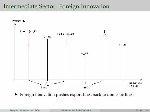
Intermediate Sector: Foreign Innovation
I Foreign innovation pushes export lines back to domestic lines.
I Foreign innovation can also steal a domestic product.
Benguria, Matsumoto and Saffie Productivity and Trade Dynamics Model 6
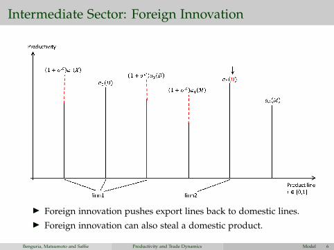
Intermediate Sector: Foreign Innovation
I Foreign innovation pushes export lines back to domestic lines.I Foreign innovation can also steal a domestic product.
Benguria, Matsumoto and Saffie Productivity and Trade Dynamics Model 6
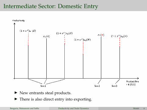
Intermediate Sector: Domestic Entry
I New entrants steal products.I There is also direct entry into exporting.
Benguria, Matsumoto and Saffie Productivity and Trade Dynamics Model 6
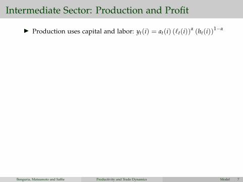
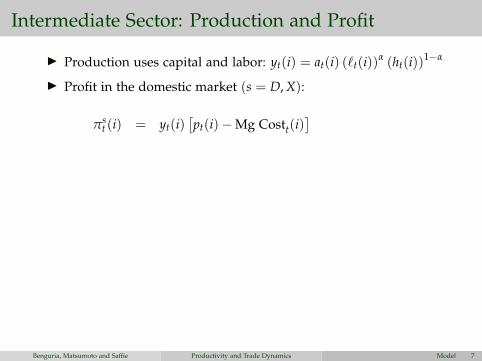
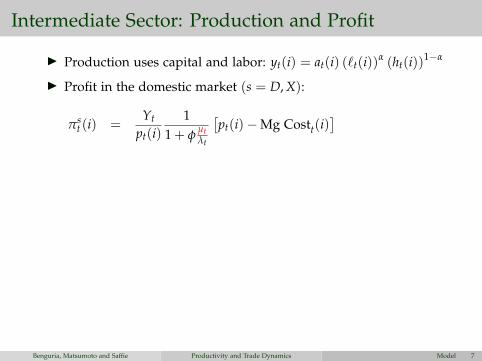
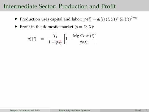
Intermediate Sector: Production and Profit
I Production uses capital and labor: yt(i) = at(i) (`t(i))α (ht(i))
1−α
I Profit in the domestic market (s = D, X):
πst (i) = [− ]
=σs
1 + σsYt
1 + φµtλt
I Profits from export lines’ foreign sales
π∗t (i) =
(1−
(1 + ξ)(RL
t)α
(Wt)1−α
(1 + σX)(RL∗
t)α
(W∗t )1−α
)︸ ︷︷ ︸
1 - relative marginal cost
Y∗t︸︷︷︸Foreigndemand
I Two key differences that are relevant during sudden stops:I Sudden stop affects domestic demand but not foreign demand.I Lower factor prices increase export profits. math
Benguria, Matsumoto and Saffie Productivity and Trade Dynamics Model 7
Intermediate Sector: Production and Profit
I Production uses capital and labor: yt(i) = at(i) (`t(i))α (ht(i))
1−α
I Profit in the domestic market (s = D, X):
πst (i) = yt(i)
[pt(i)−Mg Costt(i)
]
=σs
1 + σsYt
1 + φµtλt
I Profits from export lines’ foreign sales
π∗t (i) =
(1−
(1 + ξ)(RL
t)α
(Wt)1−α
(1 + σX)(RL∗
t)α
(W∗t )1−α
)︸ ︷︷ ︸
1 - relative marginal cost
Y∗t︸︷︷︸Foreigndemand
I Two key differences that are relevant during sudden stops:I Sudden stop affects domestic demand but not foreign demand.I Lower factor prices increase export profits. math
Benguria, Matsumoto and Saffie Productivity and Trade Dynamics Model 7
Intermediate Sector: Production and Profit
I Production uses capital and labor: yt(i) = at(i) (`t(i))α (ht(i))
1−α
I Profit in the domestic market (s = D, X):
πst (i) =
Yt
pt(i)1
1 + φµtλt
[pt(i)−Mg Costt(i)
]
=σs
1 + σsYt
1 + φµtλt
I Profits from export lines’ foreign sales
π∗t (i) =
(1−
(1 + ξ)(RL
t)α
(Wt)1−α
(1 + σX)(RL∗
t)α
(W∗t )1−α
)︸ ︷︷ ︸
1 - relative marginal cost
Y∗t︸︷︷︸Foreigndemand
I Two key differences that are relevant during sudden stops:I Sudden stop affects domestic demand but not foreign demand.I Lower factor prices increase export profits. math
Benguria, Matsumoto and Saffie Productivity and Trade Dynamics Model 7
Intermediate Sector: Production and Profit
I Production uses capital and labor: yt(i) = at(i) (`t(i))α (ht(i))
1−α
I Profit in the domestic market (s = D, X):
πst (i) =
Yt
1 + φµtλt
[1−
Mg Costt(i)pt(i)
]
=σs
1 + σsYt
1 + φµtλt
I Profits from export lines’ foreign sales
π∗t (i) =
(1−
(1 + ξ)(RL
t)α
(Wt)1−α
(1 + σX)(RL∗
t)α
(W∗t )1−α
)︸ ︷︷ ︸
1 - relative marginal cost
Y∗t︸︷︷︸Foreigndemand
I Two key differences that are relevant during sudden stops:I Sudden stop affects domestic demand but not foreign demand.I Lower factor prices increase export profits. math
Benguria, Matsumoto and Saffie Productivity and Trade Dynamics Model 7
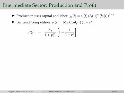
Intermediate Sector: Production and Profit
I Production uses capital and labor: yt(i) = at(i) (`t(i))α (ht(i))
1−α
I Bertrand Competition: pt(i) = Mg Costt(i) (1 + σs)
πst (i) =
Yt
1 + φµtλt
[1− 1
1 + σs
]
=σs
1 + σsYt
1 + φµtλt
I Profits from export lines’ foreign sales
π∗t (i) =
(1−
(1 + ξ)(RL
t)α
(Wt)1−α
(1 + σX)(RL∗
t)α
(W∗t )1−α
)︸ ︷︷ ︸
1 - relative marginal cost
Y∗t︸︷︷︸Foreigndemand
I Two key differences that are relevant during sudden stops:I Sudden stop affects domestic demand but not foreign demand.I Lower factor prices increase export profits. math
Benguria, Matsumoto and Saffie Productivity and Trade Dynamics Model 7
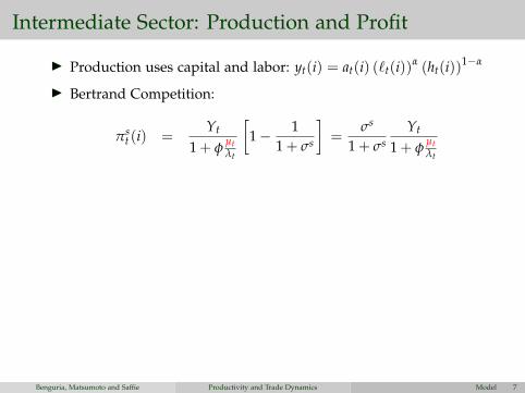
Intermediate Sector: Production and Profit
I Production uses capital and labor: yt(i) = at(i) (`t(i))α (ht(i))
1−α
I Bertrand Competition:
pt(i) = Mg Costt(i) (1 + σs)
πst (i) =
Yt
1 + φµtλt
[1− 1
1 + σs
]=
σs
1 + σsYt
1 + φµtλt
I Profits from export lines’ foreign sales
π∗t (i) =
(1−
(1 + ξ)(RL
t)α
(Wt)1−α
(1 + σX)(RL∗
t)α
(W∗t )1−α
)︸ ︷︷ ︸
1 - relative marginal cost
Y∗t︸︷︷︸Foreigndemand
I Two key differences that are relevant during sudden stops:I Sudden stop affects domestic demand but not foreign demand.I Lower factor prices increase export profits. math
Benguria, Matsumoto and Saffie Productivity and Trade Dynamics Model 7
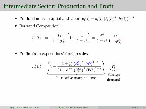
Intermediate Sector: Production and Profit
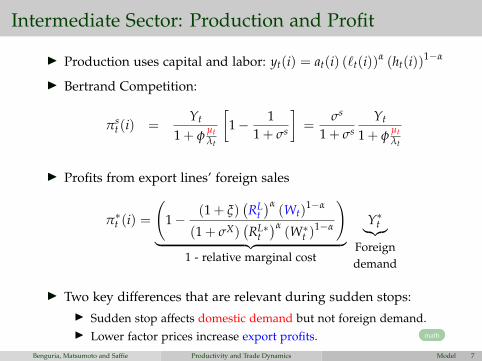
I Production uses capital and labor: yt(i) = at(i) (`t(i))α (ht(i))
1−α
I Bertrand Competition:
pt(i) = Mg Costt(i) (1 + σs)
πst (i) =
Yt
1 + φµtλt
[1− 1
1 + σs
]=
σs
1 + σsYt
1 + φµtλt
I Profits from export lines’ foreign sales
π∗t (i) =
(1−
(1 + ξ)(RL
t)α
(Wt)1−α
(1 + σX)(RL∗
t)α
(W∗t )1−α
)︸ ︷︷ ︸
1 - relative marginal cost
Y∗t︸︷︷︸Foreigndemand
I Two key differences that are relevant during sudden stops:I Sudden stop affects domestic demand but not foreign demand.I Lower factor prices increase export profits. math
Benguria, Matsumoto and Saffie Productivity and Trade Dynamics Model 7
Intermediate Sector: Production and Profit
I Production uses capital and labor: yt(i) = at(i) (`t(i))α (ht(i))
1−α
I Bertrand Competition:
pt(i) = Mg Costt(i) (1 + σs)
πst (i) =
Yt
1 + φµtλt
[1− 1
1 + σs
]=
σs
1 + σsYt
1 + φµtλt
I Profits from export lines’ foreign sales
π∗t (i) =
(1−
(1 + ξ)(RL
t)α
(Wt)1−α
(1 + σX)(RL∗
t)α
(W∗t )1−α
)︸ ︷︷ ︸
1 - relative marginal cost
Y∗t︸︷︷︸Foreigndemand
I Two key differences that are relevant during sudden stops:I Sudden stop affects domestic demand but not foreign demand.I Lower factor prices increase export profits. math
Benguria, Matsumoto and Saffie Productivity and Trade Dynamics Model 7
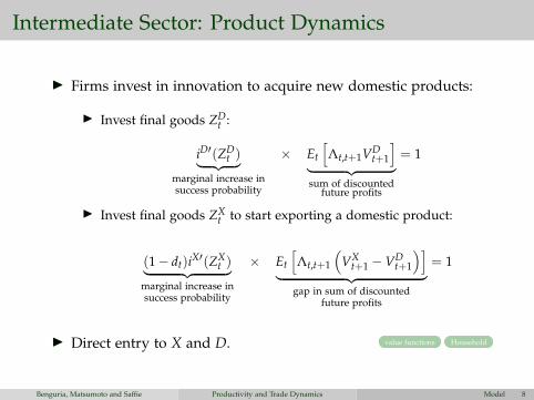
Intermediate Sector: Product Dynamics
I Firms invest in innovation to acquire new domestic products:
I Invest final goods ZDt :
iD′(ZDt )︸ ︷︷ ︸
marginal increase insuccess probability
× Et
[Λt,t+1VD
t+1
]︸ ︷︷ ︸sum of discounted
future profits
= 1
I Invest final goods ZXt to start exporting a domestic product:
(1− dt)iX′(ZXt )︸ ︷︷ ︸
marginal increase insuccess probability
× Et
[Λt,t+1
(VX
t+1 −VDt+1
)]︸ ︷︷ ︸
gap in sum of discountedfuture profits
= 1
I Direct entry to X and D. value functions Household
Benguria, Matsumoto and Saffie Productivity and Trade Dynamics Model 8
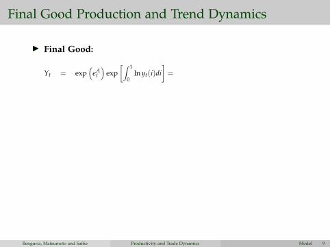
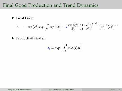
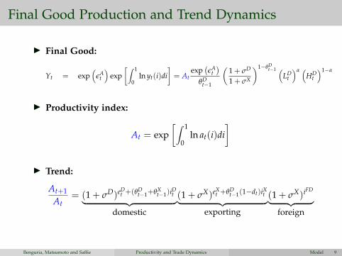
Final Good Production and Trend Dynamics
I Final Good:
(after some algebra...)
Yt = exp(
εAt
)exp
[∫ 1
0ln yt(i)di
]=
Atexp
(εA
t)
θDt−1
(1 + σD
1 + σX
)1−θDt−1 (
LDt
)α (HD
t
)1−α
I Productivity index:
At = exp[∫ 1
0ln at(i)di
]
I Trend:
At+1
At= (1 + σD)eD
t +(θDt−1+θX
t−1)iDt︸ ︷︷ ︸
domestic
(1 + σX)eXt +θD
t−1(1−dt)iXt︸ ︷︷ ︸exporting
(1 + σX)iFD︸ ︷︷ ︸foreign
Benguria, Matsumoto and Saffie Productivity and Trade Dynamics Model 9
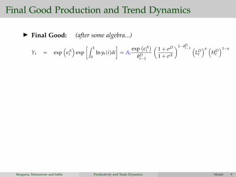
Final Good Production and Trend Dynamics
I Final Good: (after some algebra...)
Yt = exp(
εAt
)exp
[∫ 1
0ln yt(i)di
]= At
exp(εA
t)
θDt−1
(1 + σD
1 + σX
)1−θDt−1 (
LDt
)α (HD
t
)1−α
I Productivity index:
At = exp[∫ 1
0ln at(i)di
]
I Trend:
At+1
At= (1 + σD)eD
t +(θDt−1+θX
t−1)iDt︸ ︷︷ ︸
domestic
(1 + σX)eXt +θD
t−1(1−dt)iXt︸ ︷︷ ︸exporting
(1 + σX)iFD︸ ︷︷ ︸foreign
Benguria, Matsumoto and Saffie Productivity and Trade Dynamics Model 9
Final Good Production and Trend Dynamics
I Final Good:
(after some algebra...)
Yt = exp(
εAt
)exp
[∫ 1
0ln yt(i)di
]= At
exp(εA
t)
θDt−1
(1 + σD
1 + σX
)1−θDt−1 (
LDt
)α (HD
t
)1−α
I Productivity index:
At = exp[∫ 1
0ln at(i)di
]
I Trend:
At+1
At= (1 + σD)eD
t +(θDt−1+θX
t−1)iDt︸ ︷︷ ︸
domestic
(1 + σX)eXt +θD
t−1(1−dt)iXt︸ ︷︷ ︸exporting
(1 + σX)iFD︸ ︷︷ ︸foreign
Benguria, Matsumoto and Saffie Productivity and Trade Dynamics Model 9
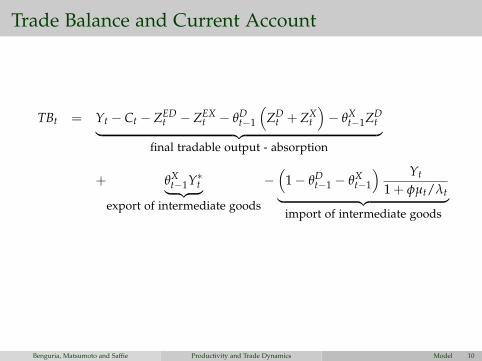
Trade Balance and Current Account
TBt = Yt − Ct − ZEDt − ZEX
t − θDt−1
(ZD
t + ZXt
)− θX
t−1ZDt︸ ︷︷ ︸
final tradable output - absorption
+ θXt−1Y∗t︸ ︷︷ ︸
export of intermediate goods
−(
1− θDt−1 − θX
t−1
) Yt
1 + φµt/λt︸ ︷︷ ︸import of intermediate goods
CAt = TBt +(
exp(εRt−1)R− 1
)Bt−1 = Bt − Bt−1
Benguria, Matsumoto and Saffie Productivity and Trade Dynamics Model 10

Quantitative Analysis
Benguria, Matsumoto and Saffie Productivity and Trade Dynamics Quantitative Analysis 10

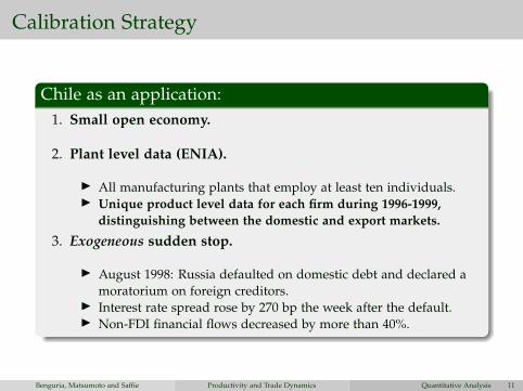
Calibration Strategy
Chile as an application:
1. Small open economy.
2. Plant level data (ENIA).
I All manufacturing plants that employ at least ten individuals.I Unique product level data for each firm during 1996-1999,
distinguishing between the domestic and export markets.
3. Exogeneous sudden stop.
I August 1998: Russia defaulted on domestic debt and declared amoratorium on foreign creditors.
I Interest rate spread rose by 270 bp the week after the default.I Non-FDI financial flows decreased by more than 40%.
Benguria, Matsumoto and Saffie Productivity and Trade Dynamics Quantitative Analysis 11

Calibration Strategy
Chile as an application:1. Small open economy.
2. Plant level data (ENIA).
I All manufacturing plants that employ at least ten individuals.I Unique product level data for each firm during 1996-1999,
distinguishing between the domestic and export markets.
3. Exogeneous sudden stop.
I August 1998: Russia defaulted on domestic debt and declared amoratorium on foreign creditors.
I Interest rate spread rose by 270 bp the week after the default.I Non-FDI financial flows decreased by more than 40%.
Benguria, Matsumoto and Saffie Productivity and Trade Dynamics Quantitative Analysis 11
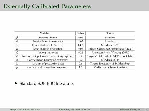
Externally Calibrated Parameters
Variable Value Source
β Discount factor 0.96 StandardR Foreign bond interest rate 1.05 Standardω Frisch elasticity 1/(ω− 1) 1.455 Mendoza (1991)α Asset share in production 0.08 Targets Capital to Output ratio (Chile)ξ Iceberg trade cost 0.21 Anderson & van Wincoop (2004)φ Fraction of input subject to working cap. req. 0.2 Targets Total credit to GDP ratio (Chile)κ Coefficient on borrowing constraint 0.2 Mendoza (2010)L Amount of productive asset 0.6 Targets Frequency of Sudden Stopsρ Concavity of innovation investment 1.5 Median value from literature
I Standard SOE RBC literature.
Benguria, Matsumoto and Saffie Productivity and Trade Dynamics Quantitative Analysis 12
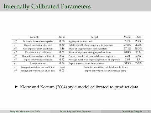
Internally Calibrated Parameters
Variable Value Target Model Data
σD Domestic innovation step size 0.06 Aggregate growth rate 2.5% 2.5%σX Export innovation step size 0.30 Relative profit of non-exporters to exporters 27.8% 26.2%ηED Non-exporter entry coefficient 1.46 Share of single-product non-exporters 37.1% 38.3%ηEX Exporter entry coefficient 0.31 Share of exporters in single-product firms 20.8% 21%ηD Domestic innovation coefficient 2.97 Average number of products by non-exporters 2.24 2.56ηX Export innovation coefficient 0.52 Average number of exported products by exporters 1.05 1.7y∗ Foreign demand 0.74 Export revenue share for exporters 30.5% 35.9%iFX Foreign innovation rate on X lines 0.23 Domestic innovation rate by domestic firms
iFD Foreign innovation rate on D lines 0.01 Export innovation rate by domestic firms
I Klette and Kortum (2004) style model calibrated to product data.
Benguria, Matsumoto and Saffie Productivity and Trade Dynamics Quantitative Analysis 13
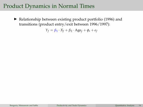
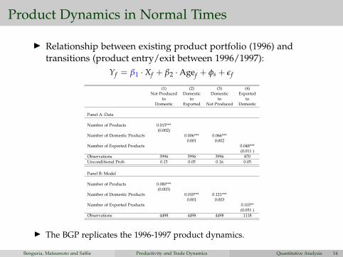
Product Dynamics in Normal Times
I Relationship between existing product portfolio (1996) andtransitions (product entry/exit between 1996/1997):
Yf = β1 ·Xf + β2 ·Agef + φs + εf
(1) (2) (3) (4)Not Produced Domestic Domestic Exported
to to to toDomestic Exported Not Produced Domestic
Panel A: Data
Number of Products 0.015***(0.002)
Number of Domestic Products 0.006*** 0.066***0.001 0.002
Number of Exported Products 0.048***(0.011 )
Observations 3996 3996 3996 870Unconditional Prob. 0.15 0.05 0.16 0.05
Panel B: Model
Number of Products 0.080***(0.003)
Number of Domestic Products 0.010*** 0.121***0.001 0.003
Number of Exported Products 0.103**(0.051 )
Observations 4498 4498 4498 1118
I The BGP replicates the 1996-1997 product dynamics.
Benguria, Matsumoto and Saffie Productivity and Trade Dynamics Quantitative Analysis 14
Firm-Size Distribution
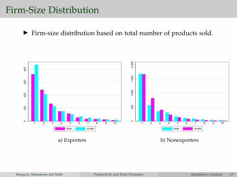
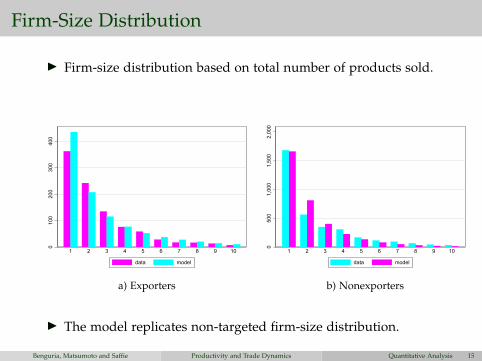
I Firm-size distribution based on total number of products sold.
010
020
030
040
0
1 2 3 4 5 6 7 8 9 10
data model
a) Exporters
050
01,
000
1,50
02,
000
1 2 3 4 5 6 7 8 9 10
data model
b) Nonexporters
I The model replicates non-targeted firm-size distribution.
Benguria, Matsumoto and Saffie Productivity and Trade Dynamics Quantitative Analysis 15
Firm-Size Distribution
I Firm-size distribution based on total number of products sold.
010
020
030
040
0
1 2 3 4 5 6 7 8 9 10
data model
a) Exporters
050
01,
000
1,50
02,
000
1 2 3 4 5 6 7 8 9 10
data model
b) Nonexporters
I The model replicates non-targeted firm-size distribution.
Benguria, Matsumoto and Saffie Productivity and Trade Dynamics Quantitative Analysis 15
Sudden Stop Dynamics: Trade Margins-.0
2-.0
10
.01
log
devi
atio
n fro
m tr
end
-4 -2 0 2 4period
a) Wage
-.02
-.01
0.0
1.0
2de
viat
ion
from
mea
n
-4 -2 0 2 4period
b) Relative Mg. Cost
-.2-.1
0.1
.2lo
g de
viat
ion
from
tren
d
-4 -2 0 2 4period
Domestic ProfitsExport Profits
c) Profits
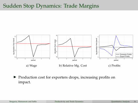
I Production cost for exporters drops, increasing profits onimpact.
Benguria, Matsumoto and Saffie Productivity and Trade Dynamics Quantitative Analysis 16
Product Transitions During Crises
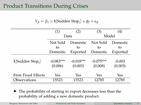
Yft = β1 × 1[Sudden Stopt] + φf + εft
(1) (2) (3) (4)Data Model
Not Sold Domestic Not Sold Domesticto to to to
Domestic Exported Domestic Exported
1[Sudden Stopt] -0.083*** -0.018*** -0.075*** -0.003(0.006) (0.003) (0.008) (0.003)
Firm Fixed Effects Yes Yes Yes YesObservations 15523 15523 12785 12785
I The probability of starting to export decreases less than theprobability of adding a new domestic product.
Benguria, Matsumoto and Saffie Productivity and Trade Dynamics Quantitative Analysis 17
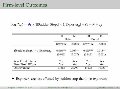
Firm-level Outcomes
log (Yft) = β1 × 1[Sudden Stopt]× 1[Exporterft] + φf + δt + εft
(1) (2) (3) (4)Data Model
Revenue Profits Revenue Profits
1[Sudden Stopt]× 1[Exporterft] 0.066*** 0.107*** 0.095*** 0.118***(0.010) (0.017) (0.011) (0.011)
Year Fixed Effects Yes Yes Yes YesFirm Fixed Effects Yes Yes Yes YesObservations 21213 20797 19022 19022
I Exporters are less affected by sudden stop than non-exporters
Benguria, Matsumoto and Saffie Productivity and Trade Dynamics Quantitative Analysis 18
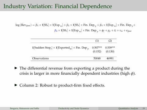
Industry Variation: Financial Dependence
log (Rev.fpmt) = β1 × 1[SSt]× 1[Exp.m] + β2 × 1[SSt]× Fin. Dep.p + β3 × 1[Exp.m]× Fin. Dep.p+
β4 × 1[SSt]× 1[Exp.m]× Fin. Dep.p + φf + ρp + δt + νm + εfpmt
(1) (2)
1[Sudden Stopt]× 1[Exportedm]× Fin. Dep.p 0.507*** 0.539***(0.152) (0.130)
Observations 50048 46981
I The differential revenue from exporting a product during thecrisis is larger in more financially dependent industries (high φ).
I Column 2: Robust to product-firm fixed effects.
Benguria, Matsumoto and Saffie Productivity and Trade Dynamics Quantitative Analysis 19
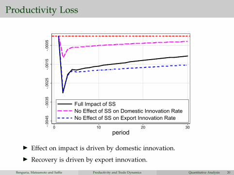
Productivity Loss
-.004
5-.0
035
-.002
5-.0
015
-.000
5
0 10 20 30period
Full Impact of SSNo Effect of SS on Domestic Innovation RateNo Effect of SS on Export Innovation Rate
I Effect on impact is driven by domestic innovation.
I Recovery is driven by export innovation.
Benguria, Matsumoto and Saffie Productivity and Trade Dynamics Quantitative Analysis 20
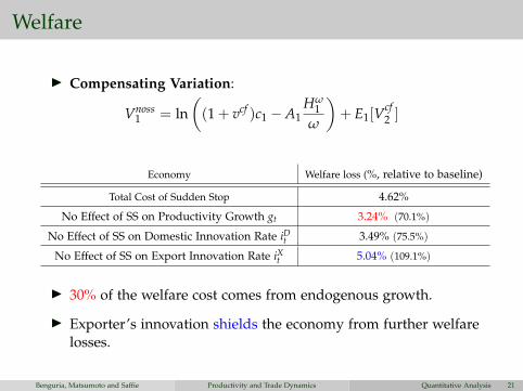
Welfare
I Compensating Variation:
Vnoss1 = ln
((1 + vcf )c1 −A1
Hω1
ω
)+ E1[V
cf2 ]
Economy Welfare loss (%, relative to baseline)
Total Cost of Sudden Stop 4.62%
No Effect of SS on Productivity Growth gt 3.24% (70.1%)
No Effect of SS on Domestic Innovation Rate iDt 3.49% (75.5%)
No Effect of SS on Export Innovation Rate iXt 5.04% (109.1%)
I 30% of the welfare cost comes from endogenous growth.
I Exporter’s innovation shields the economy from further welfarelosses.
Benguria, Matsumoto and Saffie Productivity and Trade Dynamics Quantitative Analysis 21

Conclusion
I Unified framework of endogenous sudden stops, trade and
growth.
I Calibrated to product-firm level data.
I Replicates non-targeted firm-product portfolios dynamics.
I Lower product innovation rate explains 30% of welfare cost of
sudden stops.
I Boosted export entry helps recovery and reduces welfare cost by
9%.
I Important to consider firm and trade dynamics in policy
analysis.
Benguria, Matsumoto and Saffie Productivity and Trade Dynamics Conclusion 22

Appendix
Benguria, Matsumoto and Saffie Productivity and Trade Dynamics Appendix 23
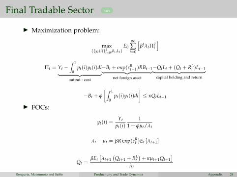
Final Tradable Sector back
I Maximization problem:
max{{yt(i)}1
i=0 ,Bt ,Lt}E0
∞
∑t=0
[βtλtΠT
t
]
Πt = Yt −∫ 1
0pt(i)yt(i)di︸ ︷︷ ︸
output - cost
−Bt + exp(εRt−1)RBt−1︸ ︷︷ ︸
net foreign asset
−QtLt + (Qt + RLt )Lt−1︸ ︷︷ ︸
capital holding and return
−Bt + φ
[∫ 1
0pt(i)yt(i)di
]≤ κQtLt−1
I FOCs:
yt(i) =Yt
pt(i)1
1 + φµt/λt
λt − µt = βR exp(εRt )Et [λt+1]
Qt =βEt
[λt+1
(Qt+1 + RL
t)+ κµt+1Qt+1
]λt
Benguria, Matsumoto and Saffie Productivity and Trade Dynamics Appendix 24
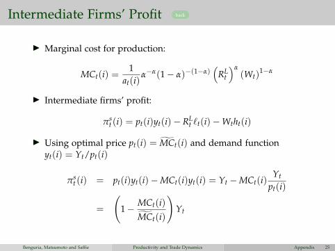
Intermediate Firms’ Profit back
I Marginal cost for production:
MCt(i) =1
at(i)α−α(1− α)−(1−α)
(RL
t
)α(Wt)
1−α
I Intermediate firms’ profit:
πst (i) = pt(i)yt(i)− RL
t `t(i)−Wtht(i)
I Using optimal price pt(i) = M̃Ct(i) and demand functionyt(i) = Yt/pt(i)
πst (i) = pt(i)yt(i)−MCt(i)yt(i) = Yt −MCt(i)
Yt
pt(i)
=
(1− MCt(i)
M̃Ct(i)
)Yt
Benguria, Matsumoto and Saffie Productivity and Trade Dynamics Appendix 25
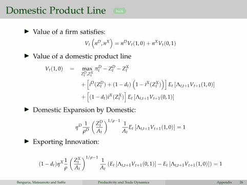
Domestic Product Line back
I Value of a firm satisfies:
Vt
(nD, nX
)= nDVt(1, 0) + nXVt(0, 1)
I Value of a domestic product line
Vt(1, 0) = maxZD
t ,ZXt
πDt − ZD
t − ZXt
+[iD(ZD
t ) + (1− dt)(
1− iX(ZXt ))]
Et [Λt,t+1Vt+1(1, 0)]
+[(1− dt)iX(ZX
t )]
Et [Λt,t+1Vt+1(0, 1)]
I Domestic Expansion by Domestic:
ηD 1ρD
(ZD
tAt
)1/ρ−1 1At
Et [Λt,t+1Vt+1(1, 0)] = 1
I Exporting Innovation:
(1− dt)ηX 1
ρ
(ZX
tAt
)1/ρ−1 1At
(Et [Λt,t+1Vt+1(0, 1)]− Et [Λt,t+1Vt+1(1, 0)]) = 1
Benguria, Matsumoto and Saffie Productivity and Trade Dynamics Appendix 26
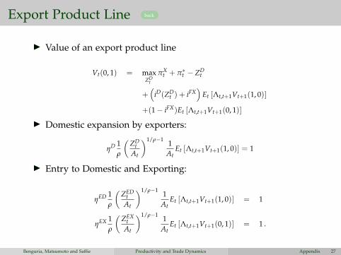
Export Product Line back
I Value of an export product line
Vt(0, 1) = maxZD
t
πXt + π∗t − ZD
t
+(
iD(ZDt ) + iFX
)Et [Λt,t+1Vt+1(1, 0)]
+(1− iFX)Et [Λt,t+1Vt+1(0, 1)]
I Domestic expansion by exporters:
ηD 1ρ
(ZD
tAt
)1/ρ−1 1At
Et [Λt,t+1Vt+1(1, 0)] = 1
I Entry to Domestic and Exporting:
ηED 1ρ
(ZED
tAt
)1/ρ−1 1At
Et [Λt,t+1Vt+1(1, 0)] = 1
ηEX 1ρ
(ZEX
tAt
)1/ρ−1 1At
Et [Λt,t+1Vt+1(0, 1)] = 1 .
Benguria, Matsumoto and Saffie Productivity and Trade Dynamics Appendix 27
Extensive Margins of Trade back
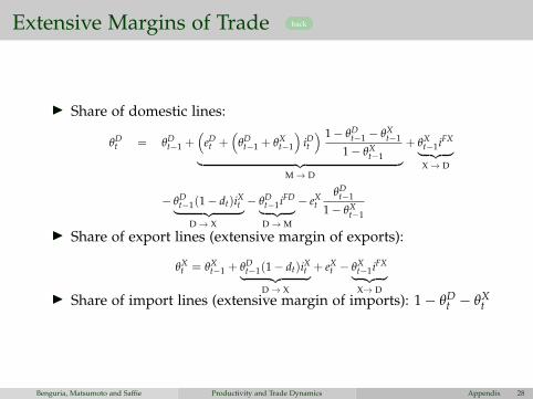
I Share of domestic lines:
θDt = θD
t−1 +(
eDt +
(θD
t−1 + θXt−1
)iDt) 1− θD
t−1 − θXt−1
1− θXt−1︸ ︷︷ ︸
M→ D
+ θXt−1iFX︸ ︷︷ ︸X→ D
− θDt−1(1− dt)iXt︸ ︷︷ ︸
D→ X
− θDt−1iFD︸ ︷︷ ︸D→ M
− eXt
θDt−1
1− θXt−1
I Share of export lines (extensive margin of exports):
θXt = θX
t−1 + θDt−1(1− dt)iXt︸ ︷︷ ︸
D→ X
+ eXt − θX
t−1iFX︸ ︷︷ ︸X→ D
I Share of import lines (extensive margin of imports): 1− θDt − θX
t
Benguria, Matsumoto and Saffie Productivity and Trade Dynamics Appendix 28
Aggregation of Intermediate Sector back
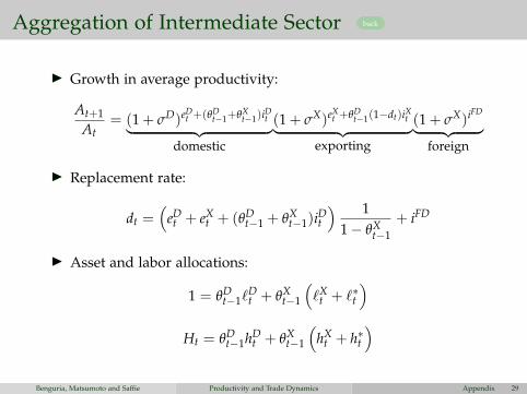
I Growth in average productivity:
At+1
At= (1 + σD)eD
t +(θDt−1+θX
t−1)iDt︸ ︷︷ ︸
domestic
(1 + σX)eXt +θD
t−1(1−dt)iXt︸ ︷︷ ︸exporting
(1 + σX)iFD︸ ︷︷ ︸foreign
I Replacement rate:
dt =(
eDt + eX
t + (θDt−1 + θX
t−1)iDt
) 11− θX
t−1+ iFD
I Asset and labor allocations:
1 = θDt−1`
Dt + θX
t−1
(`X
t + `∗t
)Ht = θD
t−1hDt + θX
t−1
(hX
t + h∗t)
Benguria, Matsumoto and Saffie Productivity and Trade Dynamics Appendix 29
Households back
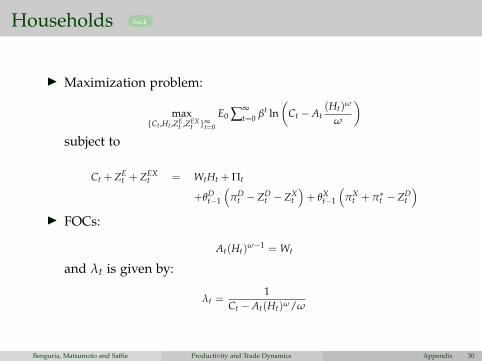
I Maximization problem:
max{Ct ,Ht ,ZE
t ,ZEXt }∞
t=0
E0 ∑∞t=0 βt ln
(Ct −At
(Ht)ω
ω
)subject to
Ct + ZEt + ZEX
t = WtHt + Πt
+θDt−1
(πD
t − ZDt − ZX
t
)+ θX
t−1
(πX
t + π∗t − ZDt
)I FOCs:
At(Ht)ω−1 = Wt
and λt is given by:
λt =1
Ct −At(Ht)ω/ω
Benguria, Matsumoto and Saffie Productivity and Trade Dynamics Appendix 30
Product Transitions
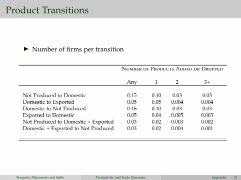
I Number of firms per transition
Number of Products Added or Dropped
Any 1 2 3+
Not Produced to Domestic 0.15 0.10 0.03 0.03Domestic to Exported 0.05 0.05 0.004 0.004Domestic to Not Produced 0.16 0.10 0.03 0.03Exported to Domestic 0.05 0.04 0.005 0.003Not Produced to Domestic + Exported 0.03 0.02 0.003 0.002Domestic + Exported to Not Produced 0.03 0.02 0.004 0.001
Benguria, Matsumoto and Saffie Productivity and Trade Dynamics Appendix 31