NBER WORKING PAPER SERIES

FROM SUDDEN STOPS TO FISHERIAN DEFLATION:QUANTITATIVE THEORY AND POLICY IMPLICATIONS

Anton KorinekEnrique G. Mendoza

Working Paper 19362http://www.nber.org/papers/w19362

NATIONAL BUREAU OF ECONOMIC RESEARCH1050 Massachusetts Avenue

Cambridge, MA 02138August 2013

We would like to acknowledge An Wang for his superb research assistance. Korinek thanks OlivierJeanne for his coauthorship and inspiration on a number of projects on which we draw in this survey.He also acknowledges financial support from CIGI/INET and the IMF. The views expressed are thoseof the author and should not be attributed to the IMF. Mendoza would like to thank Javier Bianchi,Emine Boz, Bora Durdu, Katherine Smith, Marco Terrones, and specially Guillermo Calvo for theopportunity to collaborate with them on several papers on the Sudden Stops phenomenon that servedas background material for this article. The views expressed herein are those of the authors and donot necessarily reflect the views of the National Bureau of Economic Research. Data for our eventanalysis of sudden stops, Matlab source codes and supplementary materials are available at http://www.korinek.com/suddenstops

NBER working papers are circulated for discussion and comment purposes. They have not been peer-reviewed or been subject to the review by the NBER Board of Directors that accompanies officialNBER publications.

© 2013 by Anton Korinek and Enrique G. Mendoza. All rights reserved. Short sections of text, notto exceed two paragraphs, may be quoted without explicit permission provided that full credit, including© notice, is given to the source.

From Sudden Stops to Fisherian Deflation: Quantitative Theory and Policy ImplicationsAnton Korinek and Enrique G. MendozaNBER Working Paper No. 19362August 2013, Revised September 2013JEL No. E44,F34,F41

ABSTRACT

The 1990s Sudden Stops in emerging markets were a harbinger for the 2008 global financial crisis.During Sudden Stops, countries lost access to credit, causing abrupt current account reversals, andsuffered Great Recessions. This paper reviews a class of models that yields quantitative predictionsconsistent with these observations, based on an occasionally binding credit constraint that limits debtto a fraction of the market value of incomes or assets used as collateral. Sudden Stops are infrequentevents nested within regular business cycles, and occur in response to standard shocks after periodsof expansion increase leverage ratios sufficiently. When this happens, the Fisherian debt-deflationmechanism is set in motion, as lower asset or goods prices tighten further the constraint causing furtherdeflation. This framework also embodies a pecuniary externality with important implications for macro-prudentialpolicy, because agents do not internalize how current borrowing decisions affect collateral values duringfuture financial crises.

Anton KorinekDepartment of EconomicsJohns Hopkins University440 Mergenthaler Hall3400 N. Charles StreetBaltimore, MD 21218and NBERanton@korinek.com

Enrique G. MendozaDepartment of EconomicsUniversity of Pennsylvania3718 Locust WalkPhiladelphia, PA 19104and NBERegme@sas.upenn.edu

1 Introduction

From the surface, the debacle of the Mexican economy that began in Decem-ber 20th of 1994 seemed a familiar event. Episodes of failed stabilization plansanchored on managed exchange rate regimes abound in the annals of the de-veloping world, and in Mexico in particular this was a recurrent event that hadcoincided with every presidential election since 1976. Yet, the 1994 Mexicancrash was different. It was the beginning of a new era of financial instabilityin the newly-created global financial system. It was the first of a collection ofsimilar events that swept through emerging markets wordlwide during the 1990sand that we now refer to as Sudden Stops.1

The defining characteristic of a Suddent Stop is a sharp reversal in externalcapital inflows, which is often measured by a sudden jump in the current account.At about the same time as the access to foreign financing is lost, or shortly after,the economies affl icted by Sudden Stops experience deep recessions, in manycountries the largest since the Great Depression, sharp real depreciations andcollapses in asset prices.2 Moreover, Sudden Stops typically come in clusters:The 1994 Mexican Crash triggered a Sudden Stop in Argentina in 1995 —thisspillover effect is often referred to as the Tequila Effect. In 1997-98, the EastAsian crisis engulfed Korea, Malaysia, Indonesia, Thailand, Singapore, HongKong and the Philippines, and before the 1990s were over there were SuddenStops in emerging economies across the world in Bulgaria, Chile, Colombia,Ukraine, Ecuador, Morocco, Venezuela, Russia and Turkey.3

Academic research on Sudden Stops surged starting in the second half of the1990s and led to many valuable contributions that aimed to connect the dotsbetween the financial instability at the root of Sudden Stops and their disas-trous macroeconomic consequences. Many of these contributions are collectedin prestigious conference volumes and reviewed in related surveys.4 They werealso published in leading academic journals.5 The central focus of research onSudden Stops was precisely on the intersection of macroeconomics and finance,and especially on the connection between financial instability and macroeco-nomic collapse. This was at a time when much of modern macroeconomics

1The term “Sudden Stop”was first used in this context in a paper by Dornbusch, Goldfajnand Valdés (1995), inspired by an old bankers’adage.

2 Interestingly, nominal devaluations are not a necessary condition for Sudden Stops. InArgentina in 1995 and Hong Kong in 1998, the nominal exchange rate remained constant, yetthe real exchange rate collapsed and deep recessions followed.

3Moreover, the 1998 Russian crash was followed by a sudden “flight to quality” in globalcapital markets, which caused the infamous collapse of hedge fund Long Term Capital Man-agement. Conditions in capital markets in the United States worsened to the point that theFederal Reserve was forced into lowering interest rates to ease access to liquidity and brokeringan arrangement for the orderly winding down of LTCM amongst its creditors.

4See for example the symposia issues of the Journal of International Economics (1996, 2000and 2006), the Journal of Money, Credit and Banking (2001), and the Journal of EconomicTheory (2004), as well as the NBER conference volumes edited by Krugman (2000), Edwardsand Frankel (2002), and Dooley and Frankel (2003).

5See e.g. Calvo and Mendoza (1996, 2000), Cole and Kehoe (2000), Caballero and Kr-ishnamurty (2001, 2003, 2004), Chang and Velasco (2001), Kaminsky and Reinhart (1999),Martin and Rey (2006), Lorenzoni (2008), Mendoza (2010).

2

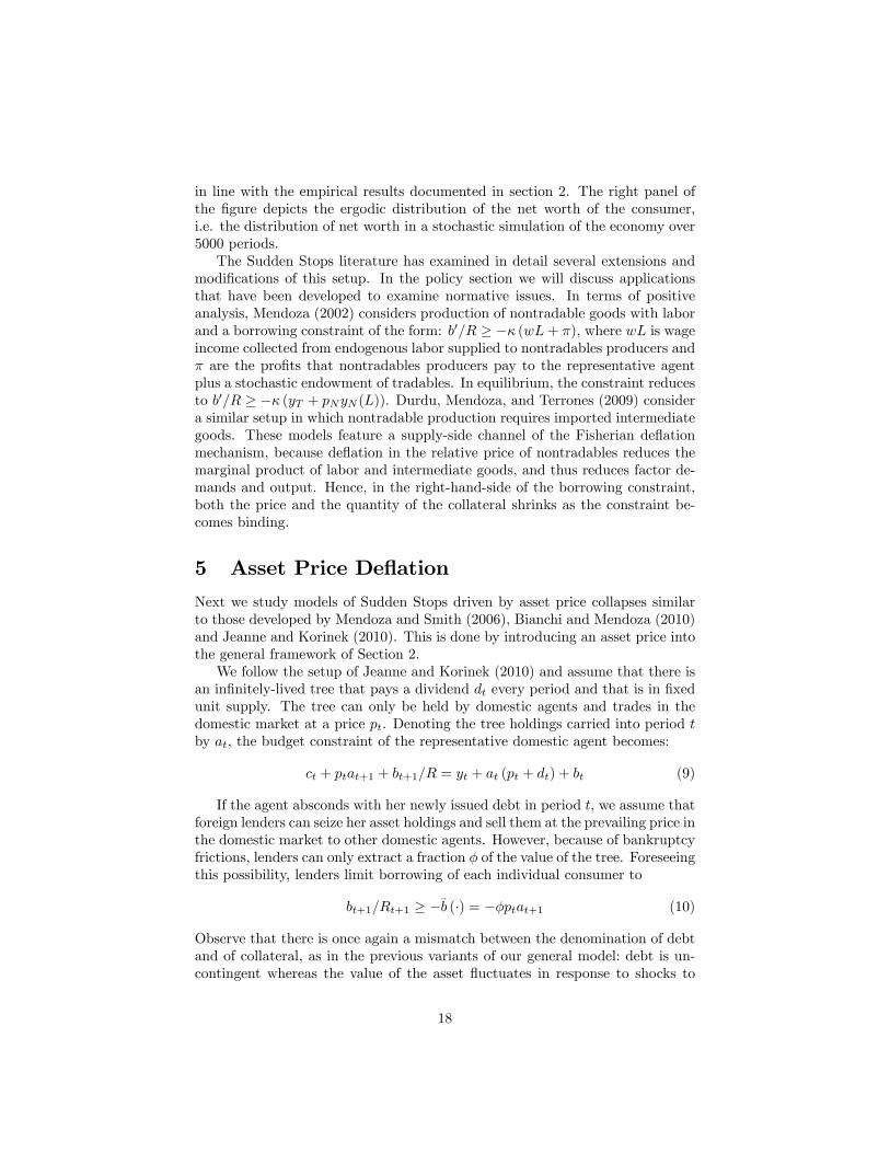
Falling Individual Spending

DecliningRelative Prices

TighteningConstraint

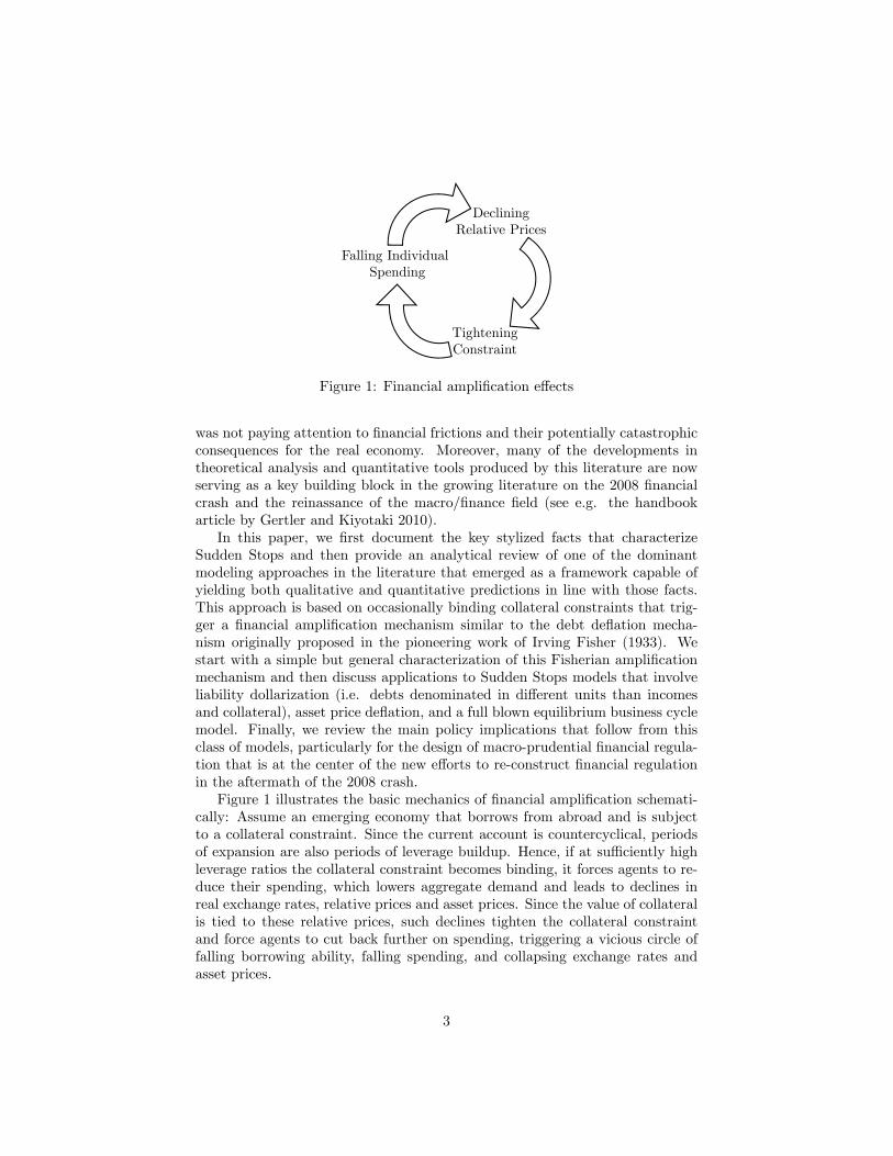
Figure 1: Financial amplification effects

was not paying attention to financial frictions and their potentially catastrophicconsequences for the real economy. Moreover, many of the developments intheoretical analysis and quantitative tools produced by this literature are nowserving as a key building block in the growing literature on the 2008 financialcrash and the reinassance of the macro/finance field (see e.g. the handbookarticle by Gertler and Kiyotaki 2010).In this paper, we first document the key stylized facts that characterize

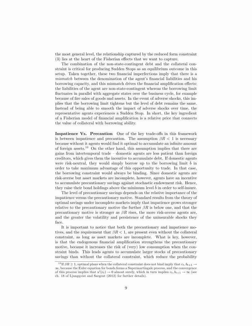
Sudden Stops and then provide an analytical review of one of the dominantmodeling approaches in the literature that emerged as a framework capable ofyielding both qualitative and quantitative predictions in line with those facts.This approach is based on occasionally binding collateral constraints that trig-ger a financial amplification mechanism similar to the debt deflation mecha-nism originally proposed in the pioneering work of Irving Fisher (1933). Westart with a simple but general characterization of this Fisherian amplificationmechanism and then discuss applications to Sudden Stops models that involveliability dollarization (i.e. debts denominated in different units than incomesand collateral), asset price deflation, and a full blown equilibrium business cyclemodel. Finally, we review the main policy implications that follow from thisclass of models, particularly for the design of macro-prudential financial regula-tion that is at the center of the new efforts to re-construct financial regulationin the aftermath of the 2008 crash.Figure 1 illustrates the basic mechanics of financial amplification schemati-

cally: Assume an emerging economy that borrows from abroad and is subjectto a collateral constraint. Since the current account is countercyclical, periodsof expansion are also periods of leverage buildup. Hence, if at suffi ciently highleverage ratios the collateral constraint becomes binding, it forces agents to re-duce their spending, which lowers aggregate demand and leads to declines inreal exchange rates, relative prices and asset prices. Since the value of collateralis tied to these relative prices, such declines tighten the collateral constraintand force agents to cut back further on spending, triggering a vicious circle offalling borrowing ability, falling spending, and collapsing exchange rates andasset prices.

3

The common thread of the applications of the Sudden Stops framework westudy, and which distinguishes it from the rest of the literature, is the emphasison studing the models’quantitative predictions using global, nonlinear numer-ical methods in experiments calibrated to data from actual economies. This isessential in order to capture the nonlinear dynamics of financial amplificationthat make financial crises so severe, the transition from states of loose financialconstraints to states with binding financial constraints, and the associated im-plications for precautionary savings. The same tools also prove to be essentialfor the use of these models to analyze normative issues and examine issues suchas the optimal design of macro-prudential financial regulation.It is worth noting that some of the issues raised in the analysis of Sudden

Stops, particularly the adjustment problems induced by a large surge in capi-tal outflows, have long been emphasized in the international economics litera-ture. One example is the well-known work of Keynes and Olin on the “transferproblem.”Their discussion centered on the contractionary forces at play in post-WW-1 Germany, which owed massive reparations to France and therefore had torun a large current account surplus and suffer from a depreciated real exchangerate. There is also a large and well-established literature on financial ampli-fication via asset prices in closed economy settings that predates the SuddenStop models with asset price deflation we examine in this paper. These modelscan be traced back to the classic article by Fisher (1933), the work of Minsky(1986), the early formal models by Bernanke and Gertler (1989) and Greenwaldand Stiglitz (1993) in simple two period settings, and the more general modelsproposed by Kiyotaki and Moore (1997), as well as quantitative applicationsof these models using perturbation methods in DSGE environments, as in thework of Carlstrom and Fuerst (1997), Bernanke, Gertler and Gilchrist (1999)and Iacoviello (2005).

2 Stylized Facts

The key defining characteristic of a Sudden Stop is a sharp, sudden reversal ininternational capital flows, which is typically measured as a sudden increase inthe current account or the balance of trade. A second empirical regularity arelarge, negative deviations from trend in the main macroeconomic aggregates(GDP, private consumption and investment) that follow the reversal in capitalflows. That is, Sudden Stops are typically associated with deep recessions. Athird characteristic are sharp changes in relative prices, including exchange ratedepreciations and declines in asset prices in both equity and housing markets.The empirical literature on Sudden Stops generally focuses on the use of

event analysis methods that apply filters to current account or net exports datato identify the dates of Sudden Stops and then constructs event windows ofmacroeconomic aggregates centered around those dates in order to study thecharacteristics of Sudden Stops.In our empirical description of Sudden Stops we follow the filter used by

4

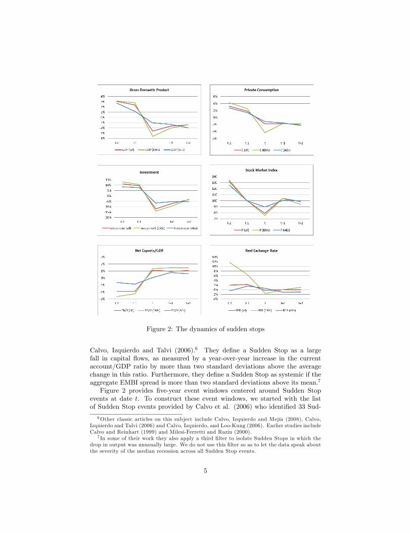
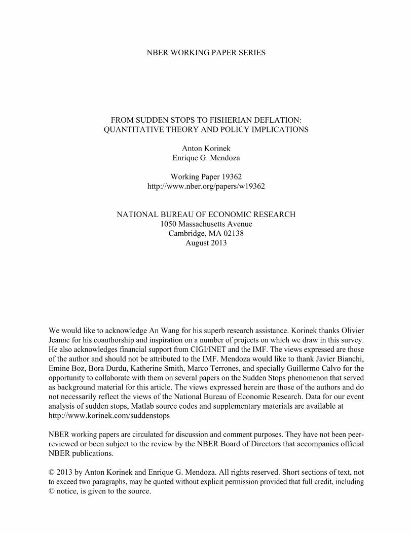
Figure 2: The dynamics of sudden stops

Calvo, Izquierdo and Talvi (2006).6 They define a Sudden Stop as a largefall in capital flows, as measured by a year-over-year increase in the currentaccount/GDP ratio by more than two standard deviations above the averagechange in this ratio. Furthermore, they define a Sudden Stop as systemic if theaggregate EMBI spread is more than two standard deviations above its mean.7

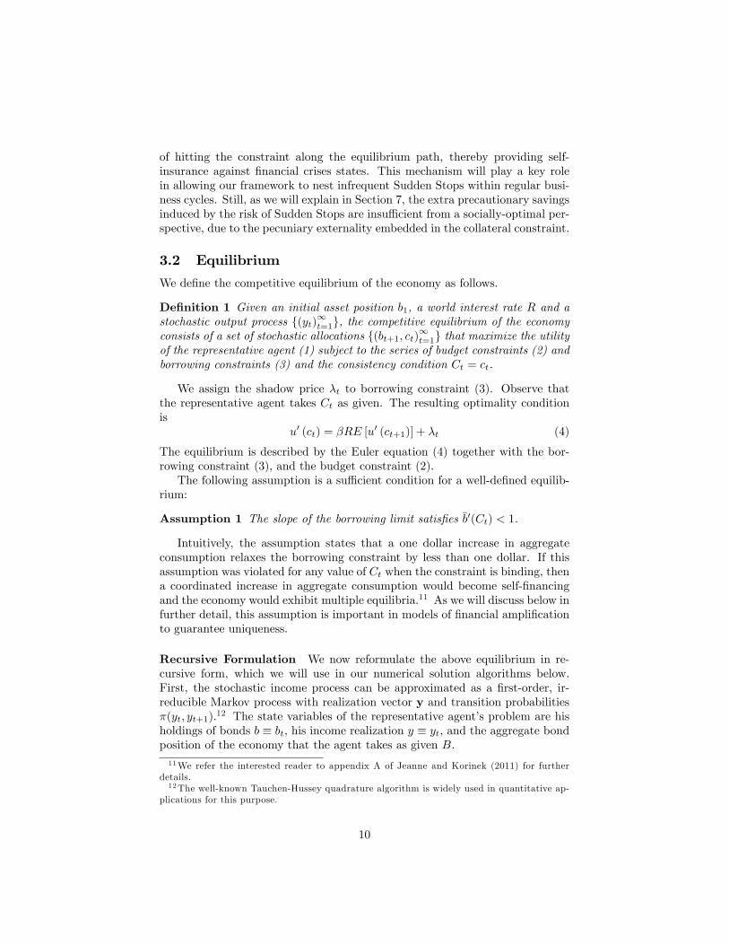
Figure 2 provides five-year event windows centered around Sudden Stopevents at date t. To construct these event windows, we started with the listof Sudden Stop events provided by Calvo et al. (2006) who identified 33 Sud-

6Other classic articles on this subject include Calvo, Izquierdo and Mejía (2008), Calvo,Izquierdo and Talvi (2006) and Calvo, Izquierdo, and Loo-Kung (2006). Earlier studies includeCalvo and Reinhart (1999) and Milesi-Ferretti and Razin (2000).

7 In some of their work they also apply a third filter to isolate Sudden Stops in which thedrop in output was unusually large. We do not use this filter so as to let the data speak aboutthe severity of the median recession across all Sudden Stop events.

5

den Stop events using data for emerging markets (EM) from 1980 to 2004. Weextended their analysis by adding emerging markets data from 2005 to 2012and including advanced economies (AE) data from 1980 to 2012, so as to cap-ture more recent Sudden Stops in both emerging markets (particularly EasternEurope) and advanced economies (especially around the 2008 crash). See Ap-pendix A for a full description of the data and the identification procedure used.The event windows use annual data from 1978 to 2012 to show the cross-countrymedians of the cyclical components of output (Y), consumption (C), investment(I), the net exports-GDP ratio (TB/Y), the real exchange rate (RER), and realstock prices (indeces re-based so that year t-1 equals 100) , where we detrendedY, C and I using the Hodrick-Prescott filter.The event windows show that Sudden Stops are preceded by periods of ex-

pansion, with GDP, consumption and investment above trend, the trade balancebelow trend, the real exchange rate appreciated, and asset prices high. The typ-ical Sudden Stop, defined as the median across all events in the data, shows areversal in the cyclical component of TB/Y of about 3 percentage points at datet. Consumption and GDP fall 2 and nearly 3 percent below trend respectively,and investment drops by 12 percentage points. A weak recovery follows, but theeconomies that go through Sudden Stops remain below trend in all three keymacro-aggregates (output, consumption and investment), and the trade balanceremains above trend two years later. Stock prices reach their lowest point alsoat date t and they are sharply lower than in the pre-Sudden-Stop peak. Twoyears later they rise somewhat but only recover about 2/5ths of their loses.The event windows also show a striking contrast in the Sudden Stop dynam-

ics across EMs and AEs. In particular, AEs do not show the inverted-J patternthat EMs display, indicating that the through of the recession is not reachedwhen the Sudden Stop hits. In fact, two years after the Sudden Stop event,output and consumption continue to move deeper below trend and investmentremains flat. Almost half of the Sudden Stop events in AEs that we identified inour sample occurred around the 2008/09 crisis and were indeed followed by anextremely slow recovery. In EMs there is also a clear and strong real apprecia-tion before the Sudden Stops hit, followed by a real exchange rate collapse andthen a modest, gradual recovery. In contrast, this pattern is absent from theSudden Stops in AEs and in the combined sample. This is in line with Mendozaand Terrones (2012) who show that credit boom events display a similar asym-metry: real appreciation followed by collapse in EMs and no noticeable patternin AEs.Mendoza (2010) highlights three other important empirical regularities of

Sudden Stops: (1) they are infrequent events nested within typical business cy-cles; (2) they generate negative skewness in macroeconomic aggregates, becausewe do not observe symmetric episodes of sudden large capital inflows coupledwith economic expansions; (3) in a standard growth accounting exercise, a sig-nificant fraction of the drop in output during a Sudden Stop is accounted forby a drop in the Solow residual rather than a decline in measured capital and

6

labor.8

Producing quantitative predictions in line with the stylized facts of SuddenStops is a tall order for standard open-economy macro DSGE models, includingreal-business-cycle (RBC) models and New Keynesian models. In these mod-els, credit markets are assumed to work as an effi cient vehicle for consumptionsmoothing and investment financing. Even if state-contingent securities are ab-sent, frictionless trading in non-state-contingent bonds allows agents to smoothout drops in output by borrowing from abroad and thus running larger currentaccount deficits. This is precisely the opposite of what we observe during Sud-den Stops: The external accounts rise sharply precisely when consumption andoutput collapse. This key observation indicates that a crucial starting point fordeveloping a framework of Sudden Stops must be to abandon the assumptionthat credit markets are perfect.9

3 General Model Structure

We start by describing a general structure for the class of models of SuddenStops that follow the Fisherian debt deflation approach. The essential featureof this structure is that borrowers are subject to a financial constraint that isitself a function of the endogenous aggregate states of the economy, which playa particularly important role as the determinants of the market prices at whichcollateral is valued. As we describe below, this endogeneity gives rise to richdynamics: it reproduces the asymmetry and amplification of negative shocksthat can be observed during sudden stops when debt levels in the economy arehigh. It also generates regular business cycle dynamics when debt levels in theeconomy are moderate and the financial constraint is loose.After describing the general setup, we impose additional structure on the

financial constraint to highlight a number of particular channels through whichthe Fisherian deflation mechanism can operate, focusing on (i) contractionaryexchange rate depreciations, (ii) contractionary asset price deflation and (iii)a general equilibrium extension of the latter in which the collateral constraintalso restricts working capital financing. This allows us to describe a full-blownequilibrium business cycle model with Sudden Stops.

3.1 Model Setup

Assume a small open economy in infinite discrete time t = 1, 2, ... The economyis inhabited by a representative agent who receives a stochastic endowmentyt every period and who values consumption ct according to a standard time-

8This is due in part to factors that bias the Solow residual as a measure of effective totalfactor productivity, TFP, such as changes in the price of imported inputs, capacity utilization,and labor hoarding—see Mendoza (2006) and Meza and Quintin (2007).

9An alternative explanation is the possibility of growth shocks as explored by Aguiar andGopinath (2007), which rely on the existence of persistent growth shocks that can be diffi cultto identify in the short samples of macro time series of several emerging economies.

7

separable expected utility function

U =∑

βtE [u (ct)] (1)

where β < 1 is the subjective discount factor and u (ct) is a standard twice-continuously differentiable, strictly concave period utility function that satisfiesthe Inada conditions.Foreign creditors are large in comparison to the small open economy and

trade one-period non-state-contingent discount bonds b with the domestic agent.International bonds carry an exogenous, time- and state-invariant price of 1/R,where R is the gross world real interest rate. As explained below, we requireβR < 1 in order to ensure a well-defined equilibrium. We denote the repaymenton the bond holdings of the home agent at the beginning of period t by btand the value of bond purchases carried as savings into the ensuing period bybt+1/R. Since in this simple setup b is the only internationally traded asset, italso defines the country’s net foreign asset (NFA) position. The period budgetconstraint is

ct + bt+1/R = yt + bt (2)

The assumption that bonds are not state-contingent implies that risk mar-kets are incomplete; thus the small open economy has an incentive to self-insure.In addition, we introduce a moral hazard problem that limits how much domes-tic consumers are able to borrow and that generates a second form of marketincompleteness: after contracting debt in period t, we assume that they have anoption to abscond. Lenders can detect this, and if they take immediate action,they can recover up to b units of the amount lent, otherwise the entire loan islost and lenders have no further recourse or means of punishment. For borrowersto refrain from absconding, lenders limit their lending to b.The borrowing limit b generally depends on the aggregate state of the econ-

omy. For example, in a booming economy with an appreciated exchange rateand elevated asset prices, lenders will find it easier to recover funds than in a de-pressed economy with low exchange rates and asset prices. It proves convenientto assume that the financial constraint depends on aggregate consumption Ct,which is taken as given by the representative agent. In equilibrium, of course,Ct = ct. In the setting described so far, Ct serves as a suffi cient statistic for ag-gregate demand and relative prices in the economy. We express the dependenceof the borrowing constraint on aggregate conditions by assuming the functionalform:

bt+1/R ≥ −b (Ct) (3)

where b′ (Ct) > 0, i.e. higher aggregate consumption increases borrowing ca-pacity. In the following two sections, we will examine variants of this settingbased on relative price changes that are associated with declines in aggregateconsumption: we will describe Fisherian models in which falling consumptionleads to real exchange rate depreciations and asset price declines. We will alsoallow for additional variables to affect the borrowing limit of domestic agents,such as individual holdings of assets or individual production plans. However, at

8

the most general level, the relationship captured by the reduced form constraint(3) lies at the heart of the Fisherian effects that we want to capture.The combination of the non-state-contingent debt and the collateral con-

straint is critical for producing Sudden Stops as an equilibrium outcome in thissetup. Taken together, these two financial imperfections imply that there is amismatch between the denomination of the agent’s financial liabilities and hisborrowing capacity, and this mismatch drives the financial amplification effects:the liabilities of the agent are non-state-contingent whereas the borrowing limitfluctuates in parallel with aggregate states over the business cycle, for examplebecause of fire sales of goods and assets. In the event of adverse shocks, this im-plies that the borrowing limit tightens but the level of debt remains the same.Instead of being able to smooth the impact of adverse shocks over time, therepresentative agents experiences a Sudden Stop. In short, the key ingredientof a Fisherian model of financial amplification is a relative price that connectsthe value of collateral with borrowing ability.

Impatience Vs. Precaution One of the key trade-offs in this frameworkis between impatience and precaution. The assumption βR < 1 is necessarybecause without it agents would find it optimal to accumulate an infinite amountof foreign assets.10 On the other hand, this assumption implies that there aregains from intertemporal trade —domestic agents are less patient than foreigncreditors, which gives them the incentive to accumulate debt. If domestic agentswere risk-neutral, they would simply borrow up to the borrowing limit b inorder to take maximum advantage of this opportunity to trade. In that case,the borrowing constraint would always be binding. Since domestic agents arerisk-averse but asset markets are incomplete, however, agents have an incentiveto accumulate precautionary savings against stochastic endowment risk. Hence,they raise their bond holdings above the minimum level b in order to self-insure.The level of precautionary savings depends on the relative importance of the

impatience versus the precautionary motive. Standard results from the theory ofoptimal savings under incomplete markets imply that impatience grows strongerrelative to the precautionary motive the further βR is below one, and that theprecautionary motive is stronger as βR rises, the more risk-averse agents are,and the greater the volatility and persistence of the uninsurable shocks theyface.It is important to notice that both the precautionary and impatience mo-

tives, and the requirement that βR < 1, are present even without the collateralconstraint, as long as asset markets are incomplete. What is key, however,is that the endogenous financial amplification strengthens the precautionarymotive, because it increases the risk of (very) low consumption when the con-straint binds. This leads agents to accumulate larger stocks of precautionarysavings than without the collateral constraint, which reduce the probability

10 If βR ≥ 1, optimal plans when the collateral constraint does not bind imply that ct, bt+1 →∞, because the Euler equation for bonds forms a Supermartingale process, and the convergenceof this process implies that u′(ct)→ 0 almost surely, which in turn implies ct, bt+1 →∞ (seech. 18 of Ljungqvist and Sargent (2012) for further details).

9

of hitting the constraint along the equilibrium path, thereby providing self-insurance against financial crises states. This mechanism will play a key rolein allowing our framework to nest infrequent Sudden Stops within regular busi-ness cycles. Still, as we will explain in Section 7, the extra precautionary savingsinduced by the risk of Sudden Stops are insuffi cient from a socially-optimal per-spective, due to the pecuniary externality embedded in the collateral constraint.

3.2 Equilibrium

We define the competitive equilibrium of the economy as follows.

Definition 1 Given an initial asset position b1, a world interest rate R and astochastic output process (yt)∞t=1, the competitive equilibrium of the economyconsists of a set of stochastic allocations (bt+1, ct)

∞t=1 that maximize the utility

of the representative agent (1) subject to the series of budget constraints (2) andborrowing constraints (3) and the consistency condition Ct = ct.

We assign the shadow price λt to borrowing constraint (3). Observe thatthe representative agent takes Ct as given. The resulting optimality conditionis

u′ (ct) = βRE [u′ (ct+1)] + λt (4)

The equilibrium is described by the Euler equation (4) together with the bor-rowing constraint (3), and the budget constraint (2).The following assumption is a suffi cient condition for a well-defined equilib-

rium:

Assumption 1 The slope of the borrowing limit satisfies b′(Ct) < 1.

Intuitively, the assumption states that a one dollar increase in aggregateconsumption relaxes the borrowing constraint by less than one dollar. If thisassumption was violated for any value of Ct when the constraint is binding, thena coordinated increase in aggregate consumption would become self-financingand the economy would exhibit multiple equilibria.11 As we will discuss below infurther detail, this assumption is important in models of financial amplificationto guarantee uniqueness.

Recursive Formulation We now reformulate the above equilibrium in re-cursive form, which we will use in our numerical solution algorithms below.First, the stochastic income process can be approximated as a first-order, ir-reducible Markov process with realization vector y and transition probabilitiesπ(yt, yt+1).12 The state variables of the representative agent’s problem are hisholdings of bonds b ≡ bt, his income realization y ≡ yt, and the aggregate bondposition of the economy that the agent takes as given B.11We refer the interested reader to appendix A of Jeanne and Korinek (2011) for further

details.12The well-known Tauchen-Hussey quadrature algorithm is widely used in quantitative ap-

plications for this purpose.

10

The optimal plans of the representative agent solve the Bellman equation

V (b, y;B) = maxb′

u(y − b′

R+ b

)+ β

∑y′

π(y, y′)V (b′, y′;B′)

s.t.

b′

R≥ −b (C)

where B′ = H(B, y), C = y − B′

R+B

The agent chooses b′ taking as given both the aggregate state B and a con-jectured law of motion H(B, y). Together, the two pin down aggregate con-sumption and determine b (C). The law of motion H(B, y) determines howthe agent’s expectations about the aggregate state variable B, aggregate con-sumption C and thus the borrowing capacity of the economy will evolve in thefuture.For a given H(B, y), the solution to the above problem is given by a policy

function b′ (b, y;B). In a rational expectations equilibrium, however, we alsorequire that the conjectured law of motion of B must match the actual oneimplied by the policy function: H(B, y) = b′ (B, y;B) identically in B.

Definition 2 (Recursive Equilibrium) The recursive equilibrium is definedby the policy function b′ (b, y;B) and associated value function V (b, y;B) suchthat (a) they solve the above Bellman equation and (b) the rational expectationsequilibrium condition holds H(B, y) = b′ (B, y;B) identically in B.

To keep the notation simple, we will denote the resulting policy function ofthe recursive equilibrium as b′ (b, y) , omitting the aggregate state that becomesredundant once condition (b) holds. In general, recursive equilibria of this formdo not have explicit closed-form solutions, except in special cases like the perfect-foresight example we study next. Several global, nonlinear numerical solutionmethods can be used to solve models in this class. In Appendix A we providean example based on an endogenous gridpoints method along with a samplecalibration and source code.13

3.3 Amplification: A Deterministic Example

We illustrate the potential for amplification in this class of models by firstfocusing on a deterministic setup with constant income (yt = y) βR = 1. Giventhese assumptions, there are two possibilities for how equilibrium is determined,depending on the initial asset position of the representative consumer b1.

13Algorithms that solve recursive formulations of the optimality conditions, instead of solv-ing directly Bellman equations like the one above, have the advantage that they can imposethe rational expectations equilibrium condition directly, and thus sidestep the need to iterateto convergence on actual and conjectured laws of motion of aggregate states.

11

Unconstrained Equilibrium For suffi ciently high period 1 bond holdingsb1, the borrowing constraint is loose in period 1 and in all following periods.The model collapses to a standard Friedman-style permanent income model ofconsumption with perfectly smooth consumption ct = y + (1− β) b1, whereconsumption is a fraction 1 − β of wealth, defined as the present discountedvalue of income plus initial net worth, which reduces to w ≡ y/(1− β) + b1.Observe that, since the model is fully stationary, bond holdings in all future

periods are a strictly increasing function of initial bond holdings: bt+s = b1∀s.Hence, a one-dollar increase in initial bond holdings is reflected one-for-one infuture bond holdings dbt/db1 = 1, and since w increases by b1 consumptionrises by the fraction 1 − β. In short, the increase in wealth is spread out overthe indefinite future and there is no amplification. Intertemporal markets playa stabilizing role by allowing consumers to smooth the consumption effect ofchanges in net worth over time. Moreover, instead of thinking of shocks toinitial net worth, we could do the analysis using wealth neutral shocks to date-1income, such that y1 falls and yt+s increases to keep w unchanged. Intertemporalmarkets would play the same role to keep consumption unchanged (see Mendoza(2005)).

Constrained Equilibrium The unconstrained equilibrium is feasible if theinitial bond holdings satisfy

b1 ≥ −b (y + (1− β) b1)

Since bt+s = b1∀s, this condition guarantees that the same property applies toall the sequence of optimal choices of future bond holdings. Given assumption1, there is a unique cut-off value of b1 for which this equation is satisfied withequality. Below this threshold, for b1 < b1, the financial constraint is binding inperiod 1 and new borrowing is given by b2/R = −b (C1) > b1.Putting together the unconstrained and constrained cases, borrowing b2/R

is given by whichever is lower — the unconstrained debt b2/R = b1/R or theconstrained debt level b (C1). Hence the budget constraint yields C1 as thesolution to the implicit equation

C1 = c1 (C1) = y + b1 + minb (C1) ,−b1/R

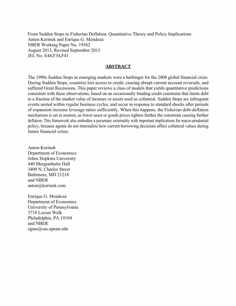
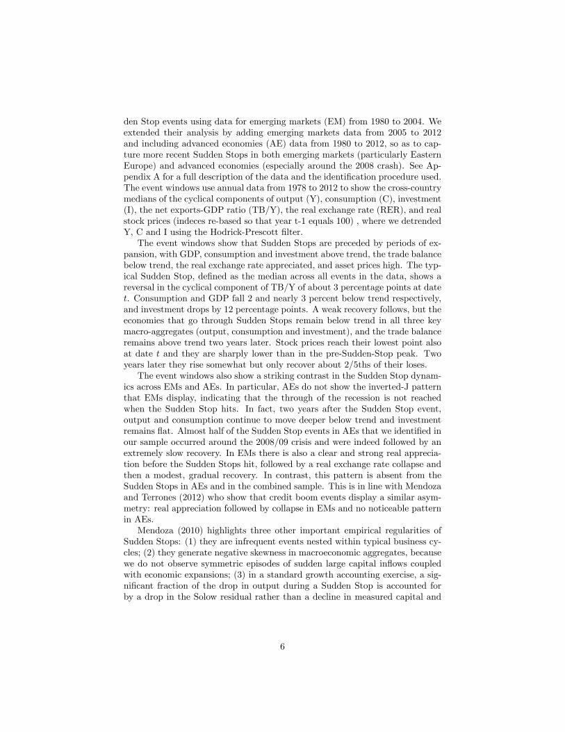
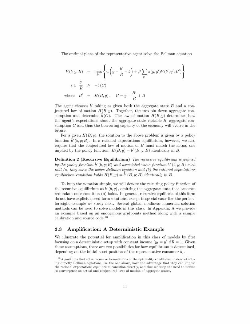
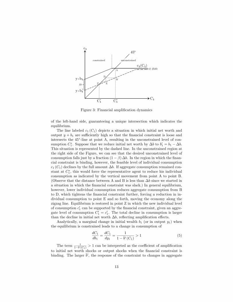
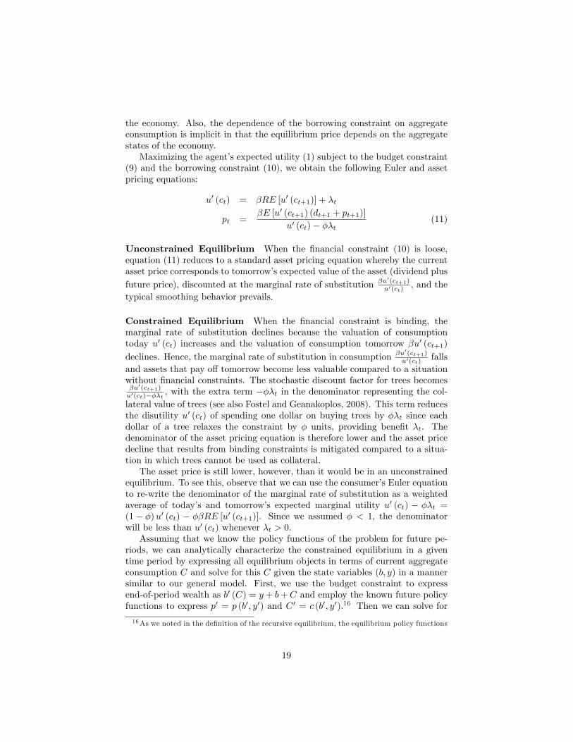
This equation is depicted in Figure 3. The first equality corresponds to the con-sistency condition of the representative agent c1 = C1 and can be represented bythe 45-line in the figure. The second equality starting with c1 (C1) = ... reflectsthat individual consumption is the minimum of its desired and its feasible levelgiven different levels of aggregate consumption C1. This equality is representedby the solid line labeled c1 (C1) that starts at the intercept y + b1. As long asthe financial constraint is binding, it starts at the intercept y + b1 + b (0) > 0and rises at slope b′ (·). When the financial constraint becomes loose, it remainsconstant at the desired level of consumption y + (1− β) b1. By Assumption1, the slope of the right-hand side in the figure is always less than the slope

12

C₁

45

y+b₁

y+b₁’

C₁C₁’

A

BD

EZ

c₁

*

c₁(C₁)constrained unconstrained

b

b

Figure 3: Financial amplification dynamics

of the left-hand side, guaranteeing a unique intersection which indicates theequilibrium.The line labeled c1 (C1) depicts a situation in which initial net worth and

output y + b1 are suffi ciently high so that the financial constraint is loose andintersects the 45-line at point A, resulting in the unconstrained level of con-sumption C∗1 . Suppose that we reduce initial net worth by ∆b to b′1 = b1 −∆b.This situation is represented by the dashed line. In the unconstrained region atthe right side of the Figure, we can see that the desired unconstrained level ofconsumption falls just by a fraction (1− β) ∆b. In the region in which the finan-cial constraint is binding, however, the feasible level of individual consumptionc1 (C1) declines by the full amount ∆b. If aggregate consumption remained con-stant at C∗1 , this would force the representative agent to reduce his individualconsumption as indicated by the vertical movement from point A to point B.(Observe that the distance between A and B is less than ∆b since we started ina situation in which the financial constraint was slack.) In general equilibrium,however, lower individual consumption reduces aggregate consumption from Bto D, which tightens the financial constraint further, forcing a reduction in in-dividual consumption to point E and so forth, moving the economy along thezigzag line. Equilibrium is restored in point Z in which the new individual levelof consumption c′1 can be supported by the financial constraint, given an aggre-gate level of consumption C ′1 = c′1. The total decline in consumption is largerthan the decline in initial net worth ∆b, reflecting amplification effects.Analytically, a marginal change in initial wealth b1 (or in output y1) when

the equilibrium is constrained leads to a change in consumption of

dC1

db1=dC1

dy1=

1

1− b′ (C1)> 1 (5)

The term 11−b′(C1)

> 1 can be interpreted as the coeffi cient of amplificationto initial net worth shocks or output shocks when the financial constraint isbinding. The larger b′, the response of the constraint to changes in aggregate

13

consumption, the stronger the amplification effects. For b′ → 1, the amplifica-tion coeffi cient becomes arbitrarily large. As we discussed under Assumption 1,we rule out the case b′ ≥ 1 because it would result in multiple equilibria.

4 Contractionary Depreciations

The first application of our general model focuses on contractionary depreci-ations under liability dollarization as proposed first in Mendoza (2002) andexplored further in Mendoza (2005). Financial liabilities in emerging marketsare often denominated in hard currencies (or tradable goods) but backed upby income or assets from the nontraded sector or the economy (see e.g. Calvo1998 and Eichengreen and Hausmann 2005). Hence, the relevant price betweenliabilities and the value of collateral is the relative price of nontraded to tradedgoods.To introduce liability dollarization, we extend our general model to include

traded and a non-traded good. The representative agent receives endowments(yT,t, yN,t) every period, and has a period utility function u (c) that dependson the composite good c = c (cT,t, cN,t) in which the two goods enter as com-plements (typically a CES aggregator). Assuming that traded goods are thenumeraire and denoting the relative price of non-traded goods by pN,t, the bud-get constraint becomes

cT,t + pN,tcN,t + bt+1/R = yT,t + pN,tyN,t + bt (6)

In case domestic agents abscond with their debts, we follow Mendoza (2005)and Korinek (2010) in assuming that international investors can seize a fractionof the market value of the endowment of consumers, resulting in a financialconstraint

bt+1/R ≥ −κ (yT,t + pN,tyN,t) (7)

Observe that the borrowing ability of consumers depends on their total in-come, which consists of both traded and non-traded goods, but their debt bt+1

is denominated entirely in traded goods in budget constraint (6).Maximizing the consumer’s expected utility subject to the budget constraint

(6) and borrowing constraint (7) and denoting the marginal utility of tradedconsumption goods by uT ≡ ∂u/∂cT and similarly for uN , we obtain the repre-sentative agent’s Euler equation and intra-temporal optimality condition

uT (cT,t, cN,t) = βRE [uT (cT,t+1, cN,t+1)] + λt

pN,t =uN (cT,t, cN,t)

uT (cT,t, cN,t)(8)

Substituting the market-clearing condition for nontradable goods cN,t = yN,t inthe second optimality condition, it follows that the exchange rate is an increas-ing function of the aggregate consumption of traded goods and the exogenousstate variable yN,t so that pN,t = pN (CT,t; yN,t). The relationship is increas-ing because traded and non-traded goods are complements, and therefore for

14

greater consumption of traded goods, the consumer would also like to increasenon-traded consumption. However, since the supply is fixed, the relative priceof non-traded goods has to go up instead to clear the market.We can rewrite the financial constraint in the form given by our general

setup asb (CT,t; yT,t, yN,t) = κ [yT,t + pN (CT,t; yN,t) yN,t]

where b is increasing in aggregate traded consumption CT,t, as in our generalmodel, and depends in addition on the exogenous state variables yT,t, yN,t. Inthis case, we need to impose the assumption b′ (CT,t; ·) < 1 to ensure a uniqueequilibrium.14 When the constraint is binding, we obtain financial amplificationdynamics that magnify the effects of shocks to the system. As in our generalmodel, for a given pair (yT,t, yN,t), we can express traded consumption under abinding financial constraint as the solution to the implicit equation

CT,t = cT,t (CT,t) = yT,t + bt + b (CT,t; yT,t, yN,t)

The graphic representation of this equation is similar to Figure 3. And whenthe representative agent experiences a shock to net worth or endowment incomeof suffi cient magnitude, similar amplification dynamics are set in motion. How-ever, the dynamics now occur through movements in the country’s real exchangerate. A negative shock forces the agent to contract consumption of traded goodsbecause he is unable to borrow the amount needed to support the unconstrainedallocation. For the economy to absorb the available supply of non-traded goods,the real exchange rate pN has to depreciate. But this reduces the value of theagent’s income and collateral, and tightens the financial constraint b, whichforces further cut-backs in consumption, and leads to a feedback loop.15 Ampli-fication effects introduce considerable volatility not only in the current accountand aggregate demand of the emerging economy, but also into the real exchangerate.

4.1 Quantitative Results

We illustrate the quantitative potential of this setup by conducting an experi-ment using the same intertemporal utility function as in the general model andfollowing Mendoza (2005) in specifying the composite good as a CES aggregator

c (cT , cN ) =[ac−µT,t + (1− a) c−µN,t

]−1/µ

. We set the expenditure share on traded

14This is satisfied as long as κp′N(cT,t

)< 1, which holds for suffi ciently low κ. If p′N is

highly convex, then truncating the debt level at some upper level Ω by defining b(cT,t; ·

)=

max−κ

[yT,t + pNyN,t

],−Ω

can guarantee that the condition b′ < 1 is satisfied globally

and that we rule out degenerate equilibria in which agents consume astronomic levels of tradedgoods in order to pump up the price of non-traded goods and relax the constraint suffi cientlyto afford the traded consumption (see Mendoza 2005).15The balance sheet effect linking constrained borrowing to tradables demand and real

depreciation is widely used in the Sudden Stops literature, starting with Calvo (1998). Incontrast, the financial amplification of this effect via the Fisherian deflation mechanism isonly at work in models of the class we review in this paper.

15

β R σ a µ κ ∆y π.96 1.03 2 1/3 .8 1/3 .03 .05

Table 1: Parameters used in sample calibration of exchange rate model

goods to a = 1/3, which corresponds closely to the weighted average of theprimary and secondary sector in GDP in our sample of emerging economies.As in Mendoza (2005), we assume an elasticity of substitution 1

1+µ = .8 anda maximum credit-to-output ratio of κ = 1/3. Finally, we assume a binaryoutput process yt ∈

yH , yL

where yH = 1 and yL = yH −∆y in which output

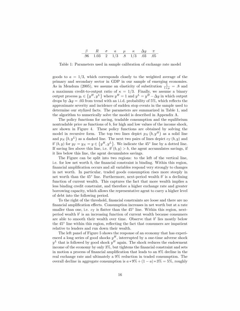
drops by ∆y = .03 from trend with an i.i.d. probability of 5%, which reflects theapproximate severity and incidence of sudden stop events in the sample used todetermine our stylized facts. The parameters are summarized in Table 1, andthe algorithm to numerically solve the model is described in Appendix A.The policy functions for saving, tradable consumption and the equilibrium

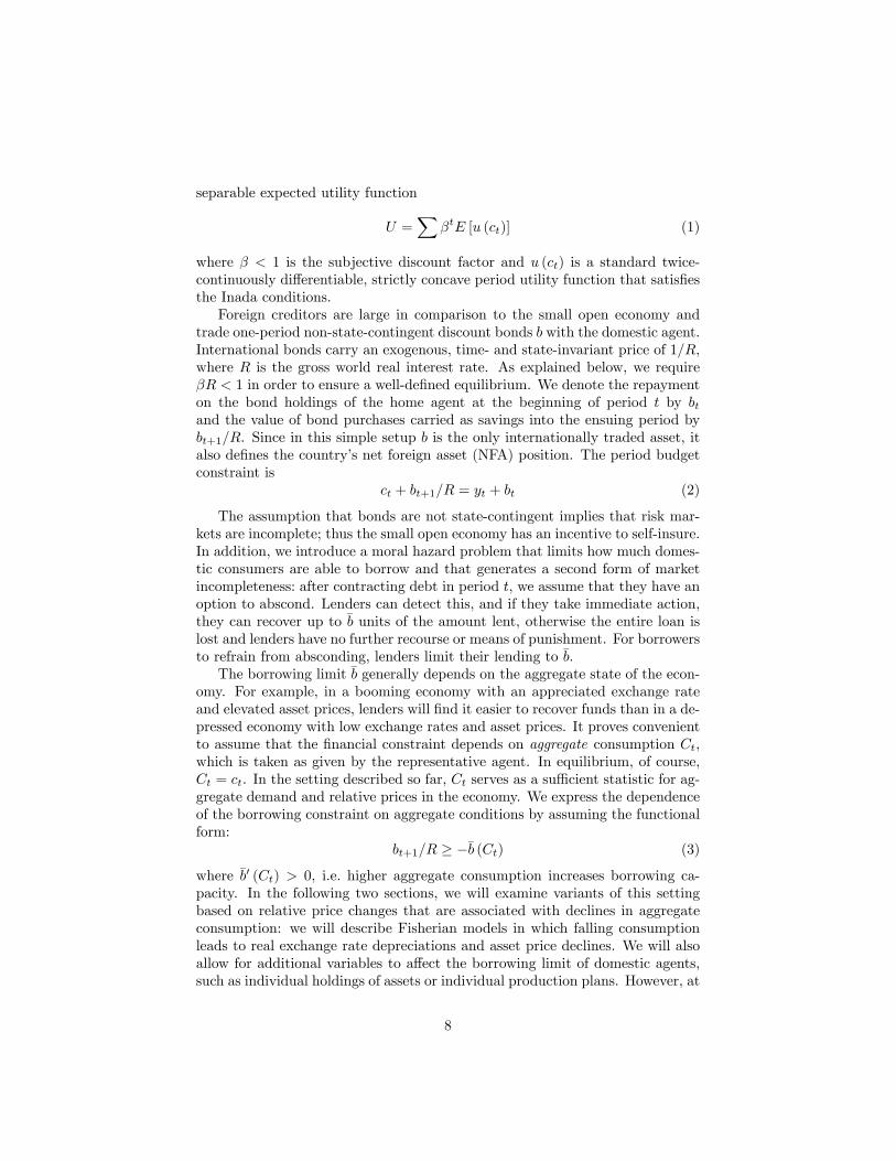
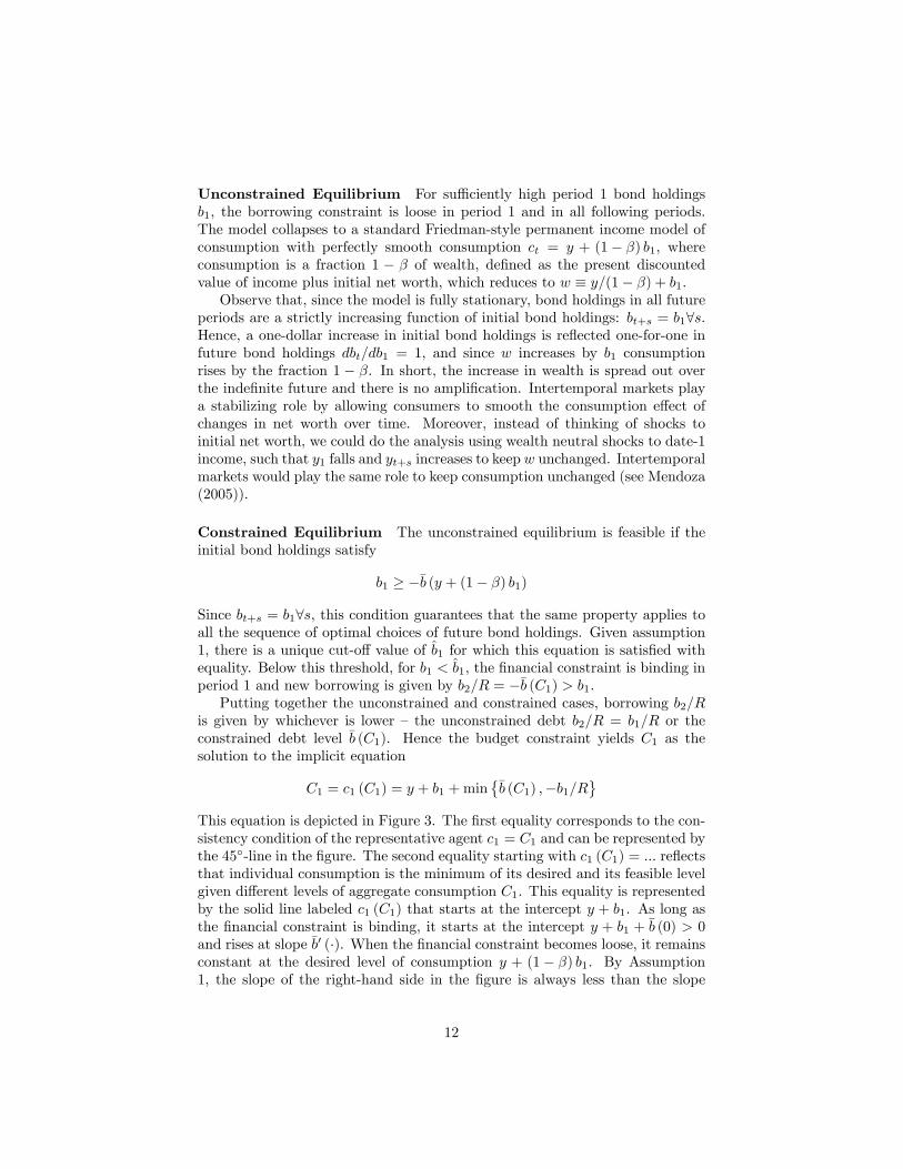
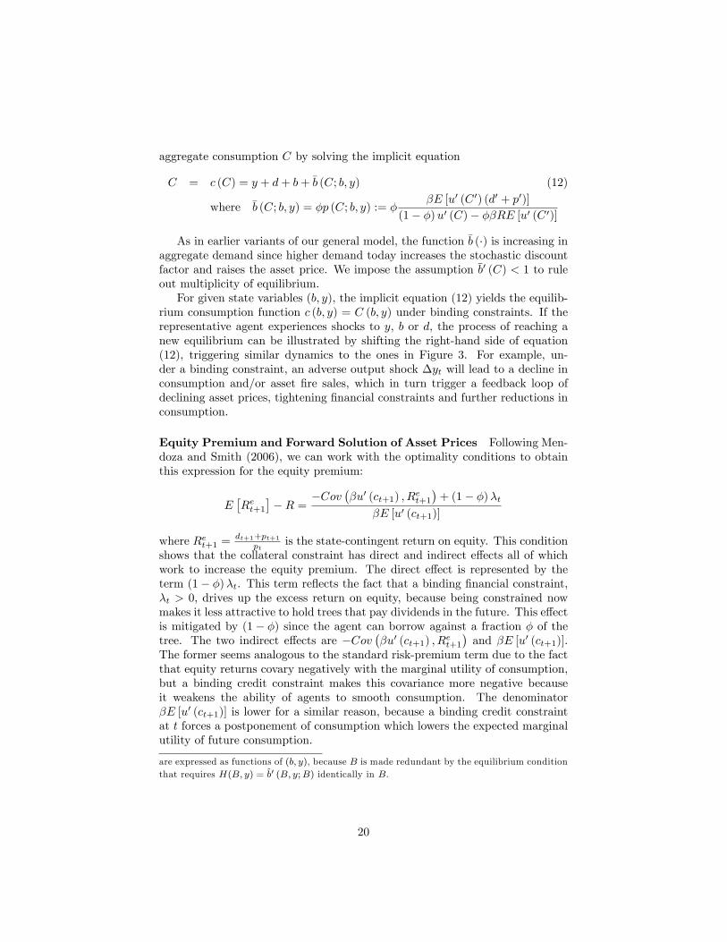
nontradable price as functions of b, for high and low values of the income shock,are shown in Figure 4. These policy functions are obtained by solving themodel in recursive form. The top two lines depict pN

(b, yH

)as a solid line

and pN(b, yL

)as a dashed line. The next two pairs of lines depict cT (b, y) and

b′ (b, y) for yT = yN = y ∈yH , yL

. We indicate the 45 line by a dotted line.

If saving lies above this line, i.e. b′ (b, y) > b, the agent accumulates savings, ifit lies below this line, the agent decumulates savings.The Figure can be split into two regions: to the left of the vertical line,

i.e. for low net worth b, the financial constraint is binding. Within this region,financial amplification occurs and all variables respond very strongly to changesin net worth. In particular, traded goods consumption rises more steeply innet worth than the 45 line. Furthermore, next-period wealth b′ is a decliningfunction of current wealth. This captures the fact that more wealth implies aless binding credit constraint, and therefore a higher exchange rate and greaterborrowing capacity, which allows the representative agent to carry a higher levelof debt into the following period.To the right of the threshold, financial constraints are loose and there are no

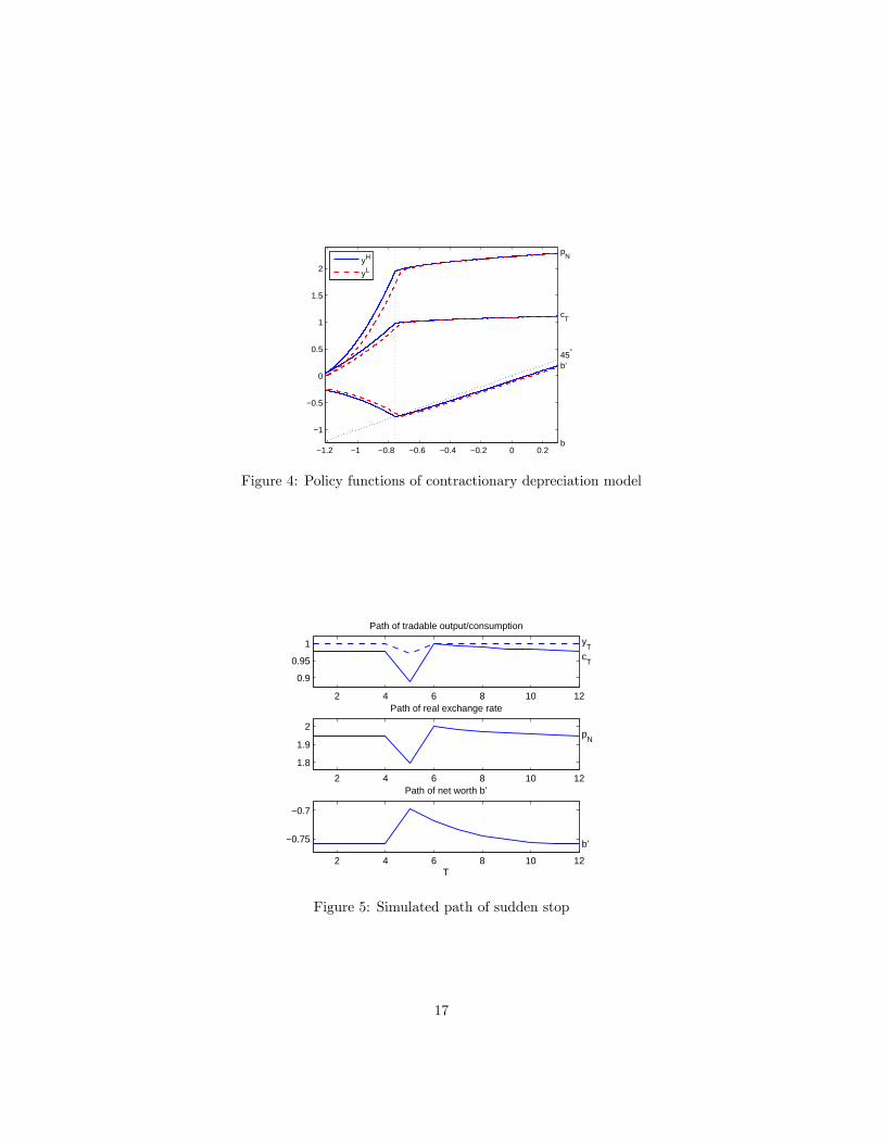
financial amplification effects. Consumption increases in net worth but at a ratesmaller than one, i.e. cT is flatter than the 45 line. Within this region, next-period wealth b′ is an increasing function of current wealth because consumersare able to smooth their wealth over time. Observe that b′ lies mostly belowthe 45 line within this region, reflecting the fact that consumers are impatientrelative to lenders and run down their wealth.The left panel of Figure 5 shows the response of an economy that has experi-

enced a long series of good shocks yH , interrupted by a one-time adverse shockyL that is followed by good shock yH again. The shock reduces the endowmentincome of the economy by only 3%, but tightens the financial constraint and setsin motion a process of financial amplification that leads to an 8% decline in thereal exchange rate and ultimately a 9% reduction in traded consumption. Theoverall decline in aggregate consumption is a ∗ 9% + (1− a) ∗ 3% = 5%, roughly

16

−1.2 −1 −0.8 −0.6 −0.4 −0.2 0 0.2

−1

−0.5

0

0.5

1

1.5

2

b’ 45°

pN

cT

b

yH

yL

Figure 4: Policy functions of contractionary depreciation model

2 4 6 8 10 12

0.9

0.95

1 yT

cT

Path of tradable output/consumption

2 4 6 8 10 12

1.8

1.9

2 p

N

Path of real exchange rate

2 4 6 8 10 12

−0.75

−0.7

b’

T

Path of net worth b’

Figure 5: Simulated path of sudden stop

17

in line with the empirical results documented in section 2. The right panel ofthe figure depicts the ergodic distribution of the net worth of the consumer,i.e. the distribution of net worth in a stochastic simulation of the economy over5000 periods.The Sudden Stops literature has examined in detail several extensions and

modifications of this setup. In the policy section we will discuss applicationsthat have been developed to examine normative issues. In terms of positiveanalysis, Mendoza (2002) considers production of nontradable goods with laborand a borrowing constraint of the form: b′/R ≥ −κ (wL+ π), where wL is wageincome collected from endogenous labor supplied to nontradables producers andπ are the profits that nontradables producers pay to the representative agentplus a stochastic endowment of tradables. In equilibrium, the constraint reducesto b′/R ≥ −κ (yT + pNyN (L)). Durdu, Mendoza, and Terrones (2009) considera similar setup in which nontradable production requires imported intermediategoods. These models feature a supply-side channel of the Fisherian deflationmechanism, because deflation in the relative price of nontradables reduces themarginal product of labor and intermediate goods, and thus reduces factor de-mands and output. Hence, in the right-hand-side of the borrowing constraint,both the price and the quantity of the collateral shrinks as the constraint be-comes binding.

5 Asset Price Deflation

Next we study models of Sudden Stops driven by asset price collapses similarto those developed by Mendoza and Smith (2006), Bianchi and Mendoza (2010)and Jeanne and Korinek (2010). This is done by introducing an asset price intothe general framework of Section 2.We follow the setup of Jeanne and Korinek (2010) and assume that there is

an infinitely-lived tree that pays a dividend dt every period and that is in fixedunit supply. The tree can only be held by domestic agents and trades in thedomestic market at a price pt. Denoting the tree holdings carried into period tby at, the budget constraint of the representative domestic agent becomes:

ct + ptat+1 + bt+1/R = yt + at (pt + dt) + bt (9)

If the agent absconds with her newly issued debt in period t, we assume thatforeign lenders can seize her asset holdings and sell them at the prevailing price inthe domestic market to other domestic agents. However, because of bankruptcyfrictions, lenders can only extract a fraction φ of the value of the tree. Foreseeingthis possibility, lenders limit borrowing of each individual consumer to

bt+1/Rt+1 ≥ −b (·) = −φptat+1 (10)

Observe that there is once again a mismatch between the denomination of debtand of collateral, as in the previous variants of our general model: debt is un-contingent whereas the value of the asset fluctuates in response to shocks to

18

the economy. Also, the dependence of the borrowing constraint on aggregateconsumption is implicit in that the equilibrium price depends on the aggregatestates of the economy.Maximizing the agent’s expected utility (1) subject to the budget constraint

(9) and the borrowing constraint (10), we obtain the following Euler and assetpricing equations:

u′ (ct) = βRE [u′ (ct+1)] + λt

pt =βE [u′ (ct+1) (dt+1 + pt+1)]

u′ (ct)− φλt(11)

Unconstrained Equilibrium When the financial constraint (10) is loose,equation (11) reduces to a standard asset pricing equation whereby the currentasset price corresponds to tomorrow’s expected value of the asset (dividend plusfuture price), discounted at the marginal rate of substitution βu′(ct+1)

u′(ct), and the

typical smoothing behavior prevails.

Constrained Equilibrium When the financial constraint is binding, themarginal rate of substitution declines because the valuation of consumptiontoday u′ (ct) increases and the valuation of consumption tomorrow βu′ (ct+1)

declines. Hence, the marginal rate of substitution in consumption βu′(ct+1)u′(ct)

fallsand assets that pay off tomorrow become less valuable compared to a situationwithout financial constraints. The stochastic discount factor for trees becomesβu′(ct+1)u′(ct)−φλt , with the extra term −φλt in the denominator representing the col-lateral value of trees (see also Fostel and Geanakoplos, 2008). This term reducesthe disutility u′ (ct) of spending one dollar on buying trees by φλt since eachdollar of a tree relaxes the constraint by φ units, providing benefit λt. Thedenominator of the asset pricing equation is therefore lower and the asset pricedecline that results from binding constraints is mitigated compared to a situa-tion in which trees cannot be used as collateral.The asset price is still lower, however, than it would be in an unconstrained

equilibrium. To see this, observe that we can use the consumer’s Euler equationto re-write the denominator of the marginal rate of substitution as a weightedaverage of today’s and tomorrow’s expected marginal utility u′ (ct) − φλt =(1− φ)u′ (ct) − φβRE [u′ (ct+1)]. Since we assumed φ < 1, the denominatorwill be less than u′ (ct) whenever λt > 0.Assuming that we know the policy functions of the problem for future pe-

riods, we can analytically characterize the constrained equilibrium in a giventime period by expressing all equilibrium objects in terms of current aggregateconsumption C and solve for this C given the state variables (b, y) in a mannersimilar to our general model. First, we use the budget constraint to expressend-of-period wealth as b′ (C) = y + b+C and employ the known future policyfunctions to express p′ = p (b′, y′) and C ′ = c (b′, y′).16 Then we can solve for

16As we noted in the definition of the recursive equilibrium, the equilibrium policy functions

19

aggregate consumption C by solving the implicit equation

C = c (C) = y + d+ b+ b (C; b, y) (12)

where b (C; b, y) = φp (C; b, y) := φβE [u′ (C ′) (d′ + p′)]

(1− φ)u′ (C)− φβRE [u′ (C ′)]

As in earlier variants of our general model, the function b (·) is increasing inaggregate demand since higher demand today increases the stochastic discountfactor and raises the asset price. We impose the assumption b′ (C) < 1 to ruleout multiplicity of equilibrium.For given state variables (b, y), the implicit equation (12) yields the equilib-

rium consumption function c (b, y) = C (b, y) under binding constraints. If therepresentative agent experiences shocks to y, b or d, the process of reaching anew equilibrium can be illustrated by shifting the right-hand side of equation(12), triggering similar dynamics to the ones in Figure 3. For example, un-der a binding constraint, an adverse output shock ∆yt will lead to a decline inconsumption and/or asset fire sales, which in turn trigger a feedback loop ofdeclining asset prices, tightening financial constraints and further reductions inconsumption.

Equity Premium and Forward Solution of Asset Prices Following Men-doza and Smith (2006), we can work with the optimality conditions to obtainthis expression for the equity premium:

E[Ret+1

]−R =

−Cov(βu′ (ct+1) , Ret+1

)+ (1− φ)λt

βE [u′ (ct+1)]

where Ret+1 = dt+1+pt+1pt

is the state-contingent return on equity. This conditionshows that the collateral constraint has direct and indirect effects all of whichwork to increase the equity premium. The direct effect is represented by theterm (1− φ)λt. This term reflects the fact that a binding financial constraint,λt > 0, drives up the excess return on equity, because being constrained nowmakes it less attractive to hold trees that pay dividends in the future. This effectis mitigated by (1− φ) since the agent can borrow against a fraction φ of thetree. The two indirect effects are −Cov

(βu′ (ct+1) , Ret+1

)and βE [u′ (ct+1)].

The former seems analogous to the standard risk-premium term due to the factthat equity returns covary negatively with the marginal utility of consumption,but a binding credit constraint makes this covariance more negative becauseit weakens the ability of agents to smooth consumption. The denominatorβE [u′ (ct+1)] is lower for a similar reason, because a binding credit constraintat t forces a postponement of consumption which lowers the expected marginalutility of future consumption.

are expressed as functions of (b, y), because B is made redundant by the equilibrium conditionthat requires H(B, y) = b′ (B, y;B) identically in B.

20

β σ φ R α ∆y.96 2 1/5 1.03 .05 .03

Table 2: Parameters used in sample calibration of asset price model

Mendoza and Smith (2006) also showed that we can obtain the followingforward solution for asset prices:

pt = E

∞∑s=t+1

[s∏

r=t+1

(Et [Rer])−1

]ds

A higher equity premium —at present or expected at any time in the futurealong the equilibrium path —reduces the present discounted value of dividends.The possibility of future Sudden Stops therefore reduces the equilibrium levelof asset prices even during good times.

5.1 Quantitative Results

We calibrate the framework in line with Jeanne and Korinek (2010) but adaptedto the setting of an emerging economy. We use the same parameters for theutility function as in our earlier calibrations, and we also pick the collateralcoeffi cient of the tree to be φ = 1/4. We assume that the dividend from the treeis a constant fraction α = dt

dt+yt= .05 of total output. This captures the share

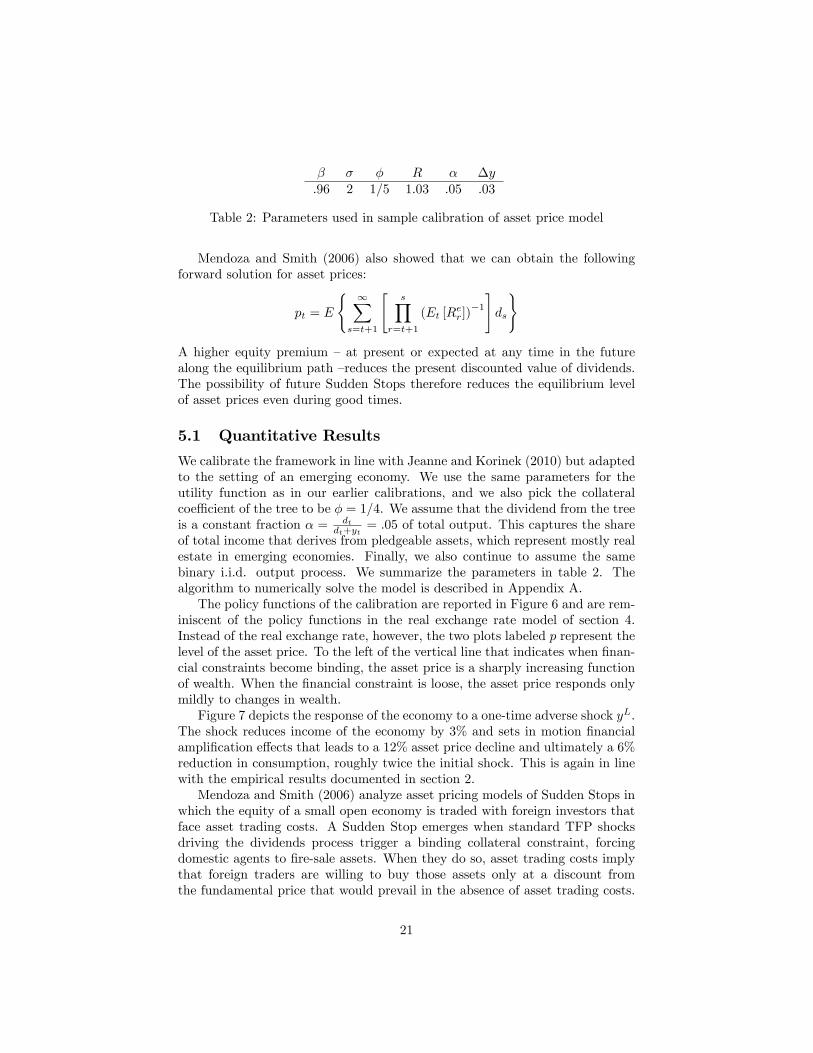
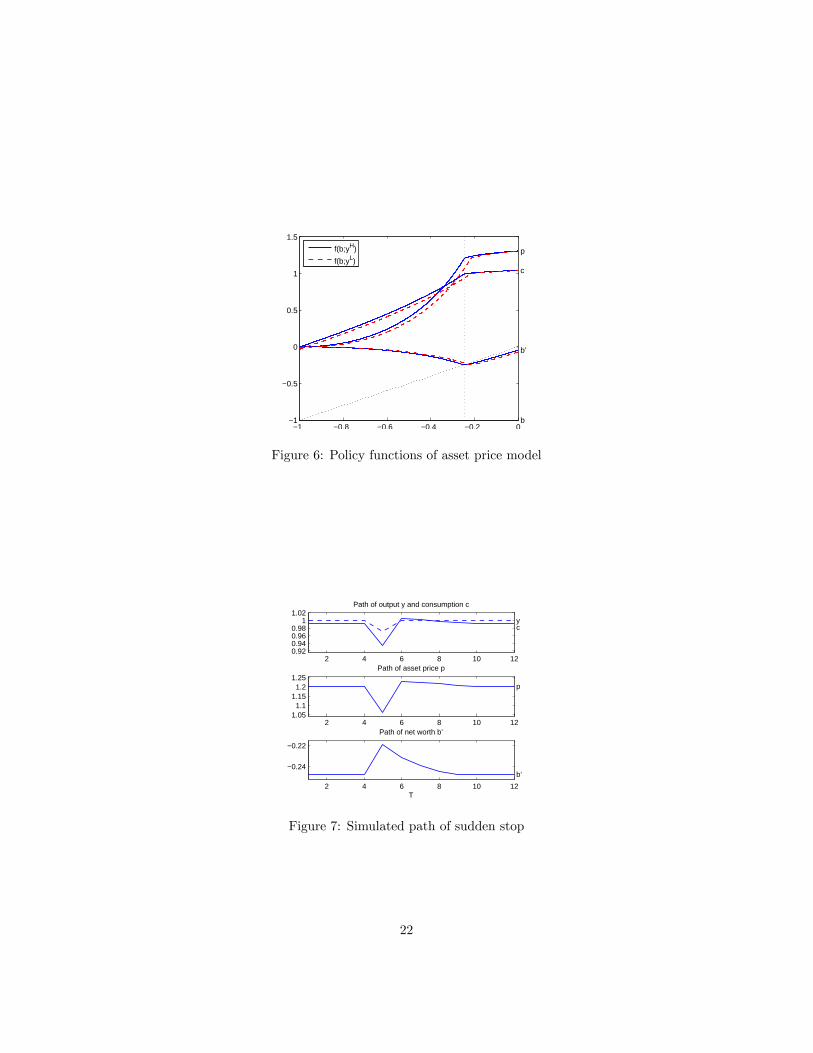
of total income that derives from pledgeable assets, which represent mostly realestate in emerging economies. Finally, we also continue to assume the samebinary i.i.d. output process. We summarize the parameters in table 2. Thealgorithm to numerically solve the model is described in Appendix A.The policy functions of the calibration are reported in Figure 6 and are rem-

iniscent of the policy functions in the real exchange rate model of section 4.Instead of the real exchange rate, however, the two plots labeled p represent thelevel of the asset price. To the left of the vertical line that indicates when finan-cial constraints become binding, the asset price is a sharply increasing functionof wealth. When the financial constraint is loose, the asset price responds onlymildly to changes in wealth.Figure 7 depicts the response of the economy to a one-time adverse shock yL.

The shock reduces income of the economy by 3% and sets in motion financialamplification effects that leads to a 12% asset price decline and ultimately a 6%reduction in consumption, roughly twice the initial shock. This is again in linewith the empirical results documented in section 2.Mendoza and Smith (2006) analyze asset pricing models of Sudden Stops in

which the equity of a small open economy is traded with foreign investors thatface asset trading costs. A Sudden Stop emerges when standard TFP shocksdriving the dividends process trigger a binding collateral constraint, forcingdomestic agents to fire-sale assets. When they do so, asset trading costs implythat foreign traders are willing to buy those assets only at a discount fromthe fundamental price that would prevail in the absence of asset trading costs.

21

−1 −0.8 −0.6 −0.4 −0.2 0−1

−0.5

0

0.5

1

1.5

b’

c

p

b

f(b;yH)

f(b;yL)

Figure 6: Policy functions of asset price model

2 4 6 8 10 120.920.940.960.98

11.02

y c

Path of output y and consumption c

2 4 6 8 10 121.05

1.11.15

1.21.25

p

Path of asset price p

2 4 6 8 10 12

−0.24

−0.22

b’

T

Path of net worth b’

Figure 7: Simulated path of sudden stop

22

The equilibrium asset price is thus determined by a combination of demandand supply forces. The supply is driven by asset fire sales, and the demandby the price elasticity of foreign asset demand, which is inversely related toasset trading costs. When calibrated to data for Mexico, the model does well attracking observed Sudden Stop dynamics in response to TFP shocks of standardmagnitudes. Obtaining large drops in the asset price, however, require a highprice elasticity of foreign asset demand.The Mendoza-Smith setup also shows that taking models with collateral

constraints into environments with multiple assets and multiple agents requiresadditional financial frictions for the Fisherian mechanism to work. Their setuprequires both short selling constraints on equity and trading costs of foreignassets. Without the former, the collateral constraint on debt can be circum-vented, and without the latter, the foreigners could buy the fire-sold assets atthe fundamental price, effectively doing away with the asset price deflation.Korinek (2011a) develops a quantitative model of a world economy that

encompasses two regions that may suffer from binding constraints and crisesdue to asset price deflation. He shows that a crisis in one region leads to lowerworld interest rates and flows of hot money to the other region, which in turnraises the vulnerability of that region to future crises. This can give rise to thephenomenon of “serial financial crises.”Mendoza (2010) and Bianchi and Mendoza (2010, 2013) consider models of

Sudden Stops involving asset price deflation in which dividends are endogenousand are affected by the collateral constraint, because working capital financingneeded to pay for a fraction of input costs is also affected by the credit constraint.This introduces a channel through which Sudden Stops affect the supply side ofthe economy. We discuss this mechanism in the ensuing section.

6 EquilibriumBusiness Cycles with Sudden Stops

In this Section, we extend the analysis to a setup in which the collateral con-straints are part of a general equilibrium business cycle model. In the absenceof credit constraints, the model reduces to one in the class of widely used real-business-cycle DSGE models of small open economies applied to both industrialand emerging economies (e.g. Mendoza 1991, 1995, Neumeyer and Perri 2005,Uribe and Yue 2006).The model is similar to other models that study the 1990semerging markets crises using credit-market frictions (e.g. Choi and Cook 2004,Cook and Devereux 2006ab, Braggion, Christiano and Roldos 2009, Gertler,Gilchrist and Natalucci 2007). These models differ from the one we review herein that they use perturbation methods to study the local quantitative impli-cations of credit frictions that are always binding, and model Sudden Stops asthe result of large, unexpected shocks to external financing or the world realinterest rate. On the other hand, it is worth noting that these models featurenominal rigidities and include a larger set of macroeconomic interactions acrosssectors than models that are tractable using global solution methods.Extending the Fisherian Sudden Stop setup to an equilibrium business cycle

23

environment requires three important modifications. First, we need to intro-duce a production technology. Mendoza (2010) uses a Cobb-Douglas technologyfor gross production that depends on capital, labor and imported intermediategoods. Second, we add endogenous capital accumulation using a Tobin’s-Qformulation of adjustment costs. Third, we assume that production requiresworking capital loans that cover a fraction of the cost of variable inputs. Thisrequires additional external financing. Thus, the collateral constraint now limitsthe total external borrowing on intertemporal bonds and working capital loansto a fraction of the market value of the accummulable physical assets that canbe pledged as collateral.With these modifications, the Fisherian debt-deflation mechanism can trig-

ger strong adverse effects on production and factor markets that are absent fromthe models we have studied so far. This occurs because the amplification mecha-nism has two important new features: First, the deflation of the price of capitalgoods (i.e. Tobin’s Q) causes a collapse in investment, which in turn affectsfuture productive capacity and factor demand. Second, the binding collateralconstraint causes as a sudden, sharp increase in the financing cost of workingcapital, captured by the shadow value on the constraint, which in turn leadsto a decline in current factor demand and production. The first effect inducespersistence in the output effects of a financial crisis, and the second causes acontemporaneous output drop when the financial crisis hits.

6.1 A Representative Firm-Household

We follow Mendoza (2010) in assuming a representative firm-household thatmakes all production and consumption decisions but acts competitively. Prefer-ences are taken from the subclass of small open economy RBC models that usethe Uzawa-Epstein utility function with an endogenous rate of time preferenceto support the existence of a well-defined long-run distribution of NFA (see Men-doza 1991 for details, and Durdu et al. 2009 for a comparison of the quantitativeimplications of this utility function with those of the standard time-separablepreferences).

E0

[ ∞∑t=0

exp

[−t−1∑τ=0

v (cτ −G (Lτ ))

]u (cτ −G (Lτ ))

]

The period utility function takes the standard CRRA form u(·) = (c−G (L))1−σ/(1−σ), which depends on the Greenwood-Hercowitz-Huffman composite good de-fined by consumption minus the disutility of labor, L. The latter is given bya constant-elasticity function G(·) = Lω/ω, where ω > 1 determines the Frischelasticity of labor supply 1/(ω − 1). This removes the wealth effect on laborsupply, which would otherwise deliver a counterfactual increase in labor supplywhen consumption falls during deep recessions. The time-preference function isdefined as v(.) = ρ ln(1 + c−G (L)), where ρ is the semi-elasticity of the rate oftime preference with respect to c−G (L) .The budget constraint of the representative firm-household is:

24

ct + it = εtkβt L

αt m

ηt − ptmt − φ(Rt − 1)(wtLt + ptmt)− qbt bt+1 + bt

where it = δkt + (kt+1 − kt)[1 + a

2

(kt+1−kt

kt

)]. The left-hand-side of the con-

straint adds up consumption and gross investment expenditures. In the defini-tion of the latter, δ denotes the depreciation rate, kt is the capital stock, and a isan adjustment-cost coeffi cient for a standard Tobin’s-Q specification of capitaladjustment costs à la Hayashi. The right-hand-side is the sum of gross produc-tion, represented by a Cobb-Douglas production function that combines capital,labor and imported inputs m, and includes also an exogenous TFP shock ε, mi-nus the cost of imported inputs (purchased at a stochastic exogenous price p),minus the interest payments on foreign working capital loans used to pay for afraction φ of the cost of variable factors, minus the cost of purchasing one-period"real" international discount bonds at an exogenous, stochastic price qb, plusthe payout on the amount of these bonds purchased the previous period. No-tice that there are three underlying real shocks driving economic fluctuations:shocks to TFP, the world relative price of imported inputs, and the world realinterest rate.The Fisherian collateral constraint is:

qbt bt+1 − φRt(wtLt + ptmt) ≥ −κqtkt+1

Hence, total external debt (one-period debt and within-period external workingcapital financing) cannot exceed the fraction κ of the market value of physicalcapital that can be pledged as collateral (qt is the market price of capital, whichis also Tobin’s Q).Two endogenous relative prices appear in the above budget and collateral

constraints: the wage rate wt and the price of capital qt. The assumption thatthe representative firm-household supports a competitive equilibrium requiresthat the agent takes these prices as given, so that they satisfy standard opti-mality conditions: the wage rate equals the marginal disutility of labor and theprice of capital equals the marginal Tobin’s Q (i.e. ∂it/∂kt, where kt is theaggregate capital stock taken as given by the representative firm-household).

6.2 Financial Amplification in a Business Cycle Model

The Fisherian deflation mechanism operates in this economy in a manner analagousto that of the endowment-economy asset pricing model reviewed earlier: Whenthe collateral constraint binds, agents fire-sell assets to meet the constraint; thislowers the price of capital, further tightening the constraint, and forces evenmore asset fire sales. The constraint introduces again direct and indirect ef-fects that increase the expected excess return on assets (i.e. capital), and has aforward-looking effect that results in qt being affected by the constraint even inperiods in which it does not bind, as long as the constraint is expected to bindwith positive probability along the equilibrium path.

25

There are two new elements to this mechanism that are crucial for integrat-ing Fisherian deflation episodes into a business cycle model: First, the asset firesales involve sales of productive assets, which results in a collapse of investmentwhen a Sudden Stop occurs. This lowers future factor demands and future out-put, thus providing a mechanism that gives persistence to the contractionaryeffects of a financial crisis. Second, the Fisherian deflation impairs access toworking capital financing and thus variable inputs for current production plans.When the constraint becomes binding, the effective marginal cost of variable in-puts suddenly rises by the factor (µt/λt)φRt, where µt and λt are the Lagrangemultipliers on the borrowing and budget constraints respectively. This mech-anism is critical for the model’s ability to generate a sudden output collapsewhen the economy hits the collateral constraint.The combination of the above two effects gives this model the ability to

produce substantial amplification and asymmetry in the responses of macroeco-nomic aggregates to the underlying real shocks driving the business cycle (seeMendoza (2010) for quantitative estimates). Amplification in the sense thatwhen the constraint binds the same size shocks generate much larger recessionsand asset price drops that when it does not, and asymmetry in the sense thatif the constraint does not bind the responses of the shocks are more tepid andin line with the behavior of a standard RBC model. Both of these propertiesare very helpful. Amplification because it is behind the model’s ability to pro-duce financial crises with realistic features, and asymmetry because it allowsthe model to produce "regular" business cycles with standard features if theconstraint does not bind. If precautionary saving is strong enough to lowerthe long-run probability of Sudden Stops to the empirically relevant range, themodel will nest infrequent financial crises within regular business cycles, and willhave an endogenous mechanism driving transitions between both that does nothinge on unusually large, unexpected exogenous shocks. Whether the model,once it is reasonably calibrated, can deliver these results is a question that canonly be answered with quantitative analaysis.

6.3 Quantitative Findings

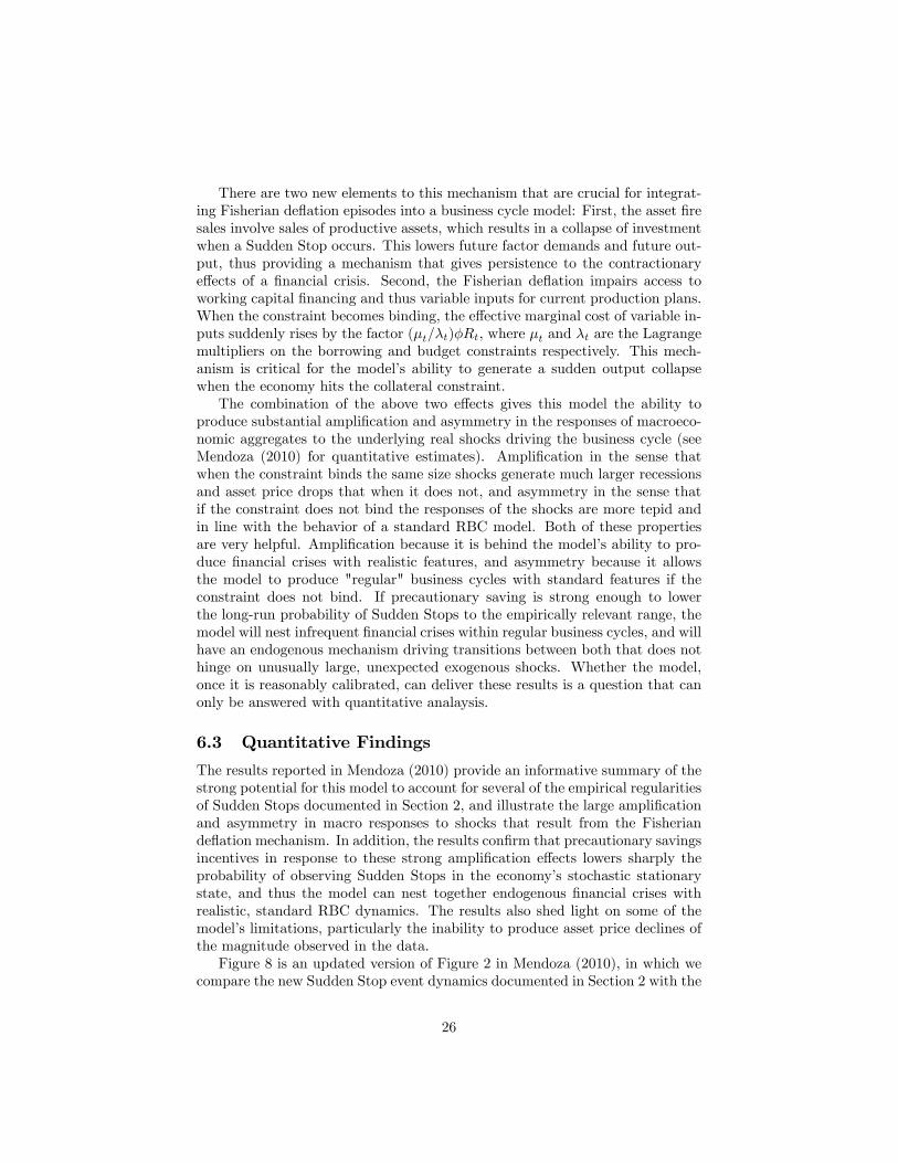
The results reported in Mendoza (2010) provide an informative summary of thestrong potential for this model to account for several of the empirical regularitiesof Sudden Stops documented in Section 2, and illustrate the large amplificationand asymmetry in macro responses to shocks that result from the Fisheriandeflation mechanism. In addition, the results confirm that precautionary savingsincentives in response to these strong amplification effects lowers sharply theprobability of observing Sudden Stops in the economy’s stochastic stationarystate, and thus the model can nest together endogenous financial crises withrealistic, standard RBC dynamics. The results also shed light on some of themodel’s limitations, particularly the inability to produce asset price declines ofthe magnitude observed in the data.Figure 8 is an updated version of Figure 2 in Mendoza (2010), in which we

compare the new Sudden Stop event dynamics documented in Section 2 with the

26

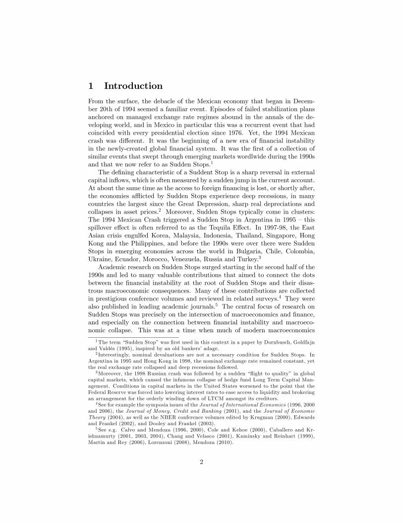
Figure 8: Sudden stop event windows in data and simulations of business cyclemodel

predicted Sudden Stop event windows produced by the model. The Figure showsthe median of Sudden Stop events in the model along with + and - one-standard-error bands, the medians from the Sudden Stop events in the data of emergingeconomies, and the realizations from Mexico’s 1995 Sudden Stop. We show thelatter because the model was calibrated to Mexican data. In particular, theproduction function parameters were set to factor shares in Mexico’s nationalaccounts. TFP shocks were calibrated to match Solow residuals constructedwith Mexican data, the interest rate shocks were set following Uribe and Yue(2006) to match the interest rate Mexico faces in world capital markets (i.e.the EMBI spread), and the shocks to the price of imported inputs were set tomatch the ratio of the price of Mexico’s imported inputs to export prices (seeMendoza (2010) for details).17The value of κ was set so as to match the observed

17These shocks are introduced into the model as a discrete Markov process that approxi-

27

frequency of Sudden Stops in the Calvo et al. (2006) dataset, which was 3.3%.This required setting κ = 0.2.As Figure 8 shows, the model does a very good job at tracking the ac-

tual Sudden Stop dynamics of GDP, consumption, investment and net exports.Moreover, these Sudden Stops are the result of standard realizations of shocksto TFP, the real interest rate and the price of imported inputs. Sudden Stopsare preceded by periods of economic expansion, and the recoveries that followare slow-paced. The model mimics very closely the declines in GDP, consump-tion, and investment in the through of the Sudden Stop, but predicts a declinein the price of capital much milder than the one observed in the data. This isbecause of the standard Tobin-Q investment setup of the model, which impliesa monotonic relationship between investment and the price of capital in whichlarge investment (price) declines occur only when the price (investment) movesslightly. Hence, without a modification that drives a wedge in this relation-ship, the model cannot do well at matching both the observed large drop ininvestment and in the price of capital at the same time.The supply-side channel operating via the collateral constraint on work-

ing capital is crucial for these favorable results. Without it the model cannotproduce amplification in production and factor demands on impact when theSudden Stop hits. GDP responds one period later, as the effect of the collapseof investment lowers future capital and future factor allocations. Moreover,without this mechanism, the optimal amount of precautionary savings (leav-ing all the other parameters at the values of the baseline calibration) results ina negligible long-run probability of observing Sudden Stops, effectively remov-ing the effect of the collateral constraint from the equilibrium dynamics. Theprobability of Sudden Stop events declines from 3.32% to 0.07%.

7 Policy Implications

The normative analysis of Sudden Stop models in the class we have reviewedhas focused on two sets of policies: First, macro-prudential or ex-ante policies,i.e. policies implemented in “good times”in order to mitigate the frequency andseverity of sudden stops in the future (e.g. Bianchi and Mendoza 2010, 2013,Jeanne and Korinek 2010b, Bianchi 2011). Second, ex-post policies aimed atdealing with financial amplification once the Fisherian mechanism is in motion(e.g. Benigno et al. 2012ab, Bianchi 2013, Jeanne and Korinek 2013b).

7.1 Macro-Prudential Policies

The fact that the value of collateral is a market price introduces a pecuniaryexternality into our Sudden Stop models because agents do not take into ac-count the effect of their individual borrowing plans on the price of collateral,which matters in particular for future states of nature in which the constraint

mates a first-order VAR process estimated with the the data on the three shocks, using theTauchen-Hussey quadrature method to construct the Markov process.

28

is binding. As a result, they borrow too much relative to what would be op-timal taking this externality into account. Alternatively, we can interpret theexternality in terms of aggregate demand: Agents do not internalize the effectsof their borrowing decisions on future aggregate demand, which is the determi-nant of future prices. They take on too much debt because they do not realizethat this implies less aggregate demand and tighter financial constraints in thefuture.This pecuniary externality is the central market-failure that justifies macro-

prudential policy intervention in the described class of models, as first notedin the theoretical work of Korinek (2007).18 The externality also has a simpleinterpretation in the theory of the second-best: If the planner reduces borrow-ing in the economy in periods before binding financial constraints occur, thisimposes a second-order cost on the economy because it constitutes a small devi-ation from optimality. When an adverse state of nature occurs next period, thepolicy relaxes the financial constraint, which has first-order welfare benefits.The approach followed in the quantitative literature on prudential policies

is to compare the features of the competitive equilibria of models similar to theones we analyzed earlier with the allocations of a social planner. This plannerchooses (or regulates) the borrowing and saving allocations of private agentswhile internalizing the pecuniary externality. In general, the results show that itis optimal for the planner to intervene in a “prudential”manner: whenever thereis a positive probability that the financial constraint may bind in the ensuingperiod, the planner reduces borrowing in the present in order to relax the futureconstraints and mitigate the associated financial amplification effects. Such anintervention improves social welfare because of the pecuniary externality.

A Prudential Planner A simple way to illustrate the implications of thepecuniary externality is to study a hypothetical prudential social planner whomaximizes the welfare of private agents by choosing a decision rule for aggregatebond holdings B′(B, y) so as to solve the following Bellman equation:

V (B, y) = maxB′u (C) + βE [V (B′, y′)]

s.t. C +B′/R = y +B

B′/R ≥ −b (C) (13)

The Euler equation of this problem is

u′ (C) = βRE[u′ (C ′) + λ′b′ (C ′)

]+ λ

[1− b′ (C)

]The difference from the optimality condition (4) of private agents is reflected inthe two terms with b′ (·), which capture that the planner internalizes the effects18A similar pecuniary externality was also described by Caballero and Krishnamurthy (2003)

and Lorenzoni (2008). In their papers, the ineffi ciency arises because financial markets areincomplete and a movement in exchange rates or asset prices that is engineered by a socialplanner generates a redistribution toward constrained agents. In our setup, by contrast, thefinancial constraint depends on prices and so a movement in relative prices directly relaxesthe financial constraint.

29

of aggregate consumption on the borrowing limit. Observe that this term ispre-multiplied by the shadow price on the borrowing constraint, i.e. relaxingthe borrowing limit is only relevant when the borrowing constraint is binding.We distinguish between two cases: when λ > 0 the credit constraint is

binding at t. In this case, the binding constraint implies that there is effectivelyno free choice variable at time t and the planner’s allocations coincide with thoseof the competitive equilibrium.In the second case, when λ = 0, the Euler equation reduces to

u′ (C) = βRE[u′ (C ′) + λ′b′ (C ′)

](14)

In this case, at date t the planner weighs the marginal utility of consumptiontoday versus the marginal utility of consumption tomorrow plus the marginalbenefit of relaxing the constraint tomorrow by increasing consumption tomor-row, captured by the term λ′b′ (C ′). This is achieved by borrowing less at t soas to transfer more consumption into t+1. If the constraint is binding with non-zero probability in some of the states attainable at t+ 1 along the equilibriumpath, then this term is positive and captures the uninternalized social benefitsof greater aggregate consumption tomorrow. This result can be proved formallyby simply comparing the Euler equation of the planner (14) when λ = 0 to theEuler equation of private agents (4).The planner can implement the optimal allocations by imposing a tax on

borrowing that corresponds to the wedge between the social and private Eulerequations. Imposing a tax τ on borrowing b′/R that is rebated lump-sum mod-ifies the Euler equation of private agents to

(1− τ)u′ (c) = βRE [u′ (c′)] + λ

In order to attain the same allocations as with the planner’s Euler equation(14), the optimal tax is:

τ =βRE

[λ′b′ (C ′)

]u′ (c)

. (15)

The tax captures the effects of higher borrowing on tightening the constraint,which is not internalized by individual agents. It is often referred to as a Pigou-vian tax because it offsets an externality. The literature has also explored howsimilar outcomes can be implemented with other instruments such as state-contingent capital requirements or loan-to-value ratios (see e.g. Bianchi 2011).Pigouvian taxes to lean against the risk of sudden stops can be interpreted

as prudential capital controls. See Korinek (2011) for a survey of a growingliterature on this topic.

Contractionary Depreciations Model The exchange rate model of Section4 imposes additional structure on the credit constraint that allows us to interpretthe externality in terms of Fisherian deflation of the real exchange rate. Inparticular, the externality term in that model can be rewritten as λ′b′ (C ′T ; ·) =λ′κp′N (C ′T ; ·) yN . In this formulation, it is clear that borrowing less in one period

30

increases aggregate consumption of traded goods in the ensuing period, whichin turn increases the price of nontradables and hence the value of collateral,relaxing the constraint by a fraction κ of the value of the collateral. Korinek(2010) and Bianchi (2011) quantify the externalities of Sudden Stops in the realexchange rate model.Korinek (2011) develops a suffi cient-statistics approach following the method-

ology of Chetty (2009), which identifies direct empirical counterparts (i.e. suf-ficient statistics) to the individual components of the tax formula (15) in orderto quantify the magnitude of externalities. He applies this procedure to theexternalities during the Indonesian crisis of 1997/98 and finds that each unit ofdollar debt that was repaid in the crisis imposed a 30 cent externality. He alsoquantifies the externalities of other financial liabilities and finds a pecking orderwhereby dollar debt imposes the largest externalities, followed by CPI-indexeddebt, local currency debt, portfolio investment and FDI, which creates the leastexternalities.19

Bianchi (2011) explores the quantitative implications of the above policyarguments using a model calibrated to the case of Argentina and finds that atax to internalize the pecuniary externality would average about 5% and wouldincrease with crisis risk. In the stochastic steady-state of the economy, theoptimal tax policy reduces the probability of a sudden stop by more than 90%.Gondo Mori (2013) introduces state-contingent assets into this framework

and shows that the opportunity to insure reduces the externalities of foreignborrowing, but does not make them disappear.

Asset Pricing Model We next consider the case for prudential policy in theasset pricing model of Section 5. In that model, the externality term in theEuler equation of the planner (14) can be expressed as λ′b′ (C ′; ·) = λφp′ (C ′; ·).Higher aggregate consumption increases the asset price and relaxes the borrow-ing constraint. The planner finds it optimal to intervene in a prudential fashionby reducing borrowing in periods when the constraint is loose but when thereis risk of binding constraints and financial amplification in the following period.Lower borrowing increases aggregate demand and asset prices in crisis times,which implies that private agents need to delever less.Bianchi and Mendoza (2010) and Jeanne and Korinek (2010b) conduct a

quantitative investigation of the above arguments.20 They calibrate their mod-els to the sudden stop experienced by the US economy in 2008, and computetaxes on borrowing that are positively correlated with leverage when the con-

19Observe that local currency debt still imposes negative externalities (of about 9 cents perdollar of debt in Korinek’s analysis) even though there is no mismatch between the denomi-nation of the debt and of the collateral. The reason is that having lower financial liabilities —no matter in which currency —implies higher aggregate traded consumption next period anda higher price of the non-traded collateral, which relaxes the financial constraint.20Korinek (2011) analyzes the externalities created by different types of financial liabilities

in a stylized model of fire sales. He finds that the externalities are higher the greater themismatch between the payoff profile of liabilities and the assets to be sold. For example,uncontingent debt imposes large externalities, whereas equity finance creates significantlysmaller externalities.

31

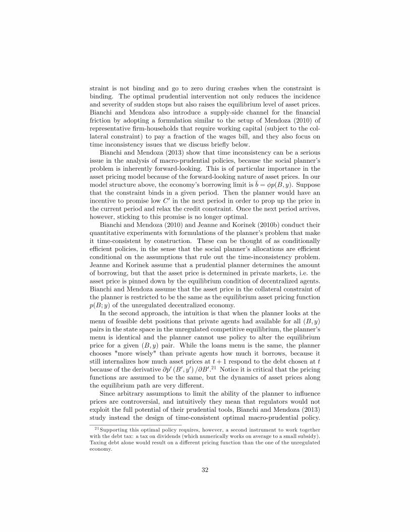
straint is not binding and go to zero during crashes when the constraint isbinding. The optimal prudential intervention not only reduces the incidenceand severity of sudden stops but also raises the equilibrium level of asset prices.Bianchi and Mendoza also introduce a supply-side channel for the financialfriction by adopting a formulation similar to the setup of Mendoza (2010) ofrepresentative firm-households that require working capital (subject to the col-lateral constraint) to pay a fraction of the wages bill, and they also focus ontime inconsistency issues that we discuss briefly below.Bianchi and Mendoza (2013) show that time inconsistency can be a serious

issue in the analysis of macro-prudential policies, because the social planner’sproblem is inherently forward-looking. This is of particular importance in theasset pricing model because of the forward-looking nature of asset prices. In ourmodel structure above, the economy’s borrowing limit is b = φp(B, y). Supposethat the constraint binds in a given period. Then the planner would have anincentive to promise low C ′ in the next period in order to prop up the price inthe current period and relax the credit constraint. Once the next period arrives,however, sticking to this promise is no longer optimal.Bianchi and Mendoza (2010) and Jeanne and Korinek (2010b) conduct their

quantitative experiments with formulations of the planner’s problem that makeit time-consistent by construction. These can be thought of as conditionallyeffi cient policies, in the sense that the social planner’s allocations are effi cientconditional on the assumptions that rule out the time-inconsistency problem.Jeanne and Korinek assume that a prudential planner determines the amountof borrowing, but that the asset price is determined in private markets, i.e. theasset price is pinned down by the equilibrium condition of decentralized agents.Bianchi and Mendoza assume that the asset price in the collateral constraint ofthe planner is restricted to be the same as the equilibrium asset pricing functionp(B; y) of the unregulated decentralized economy.In the second approach, the intuition is that when the planner looks at the

menu of feasible debt positions that private agents had available for all (B, y)pairs in the state space in the unregulated competitive equilibrium, the planner’smenu is identical and the planner cannot use policy to alter the equilibriumprice for a given (B, y) pair. While the loans menu is the same, the plannerchooses "more wisely" than private agents how much it borrows, because itstill internalizes how much asset prices at t+ 1 respond to the debt chosen at tbecause of the derivative ∂p′ (B′, y′) /∂B′.21 Notice it is critical that the pricingfunctions are assumed to be the same, but the dynamics of asset prices alongthe equilibrium path are very different.Since arbitrary assumptions to limit the ability of the planner to influence

prices are controversial, and intuitively they mean that regulators would notexploit the full potential of their prudential tools, Bianchi and Mendoza (2013)study instead the design of time-consistent optimal macro-prudential policy.

21Supporting this optimal policy requires, however, a second instrument to work togetherwith the debt tax: a tax on dividends (which numerically works on average to a small subsidy).Taxing debt alone would result on a different pricing function than the one of the unregulatedeconomy.

32

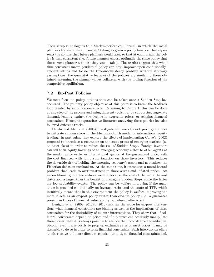
Their setup is analogous to a Markov-perfect equilibrium, in which the socialplanner chooses optimal plans at t taking as given a policy function that repre-sents the actions that future planners would take, so that at equilibrium the pol-icy is time consistent (i.e. future planners choose optimally the same policy thatthe current planner assumes they would take). The results suggest that whiletime-consistent macro prudential policy can both improve upon conditionally-effi cient setups and tackle the time-inconsistency problem without arbitraryassumptions, the quantitative features of the policies are similar to those ob-tained assuming the planner values collateral with the pricing function of thecompetitive equilibrium.

7.2 Ex-Post Policies

We next focus on policy options that can be taken once a Sudden Stop hasoccurred. The primary policy objective at this point is to break the feedbackloop created by amplification effects. Returning to Figure 1, this can be doneat any step of the process and using different tools, i.e. by supporting aggregatedemand, leaning against the decline in aggregate prices, or relaxing financialconstraints. Hence, the quantitative literature analyzing these policies has alsofollowed different tracks.Durdu and Mendoza (2006) investigate the use of asset price guarantees

to mitigate sudden stops in the Mendoza-Smith model of international equitytrading. In particular, they explore the effects of implementing Calvo’s (2002)proposal to introduce a guarantee on the asset prices of emerging markets (asan asset class) in order to reduce the risk of Sudden Stops. Foreign investorscan sell their equity holdings of an emerging economy either to other agents atthe market price or to an international agency at the guaranteed price, withthe cost financed with lump sum taxation on those investors. This reducesthe downside risk of holding the emerging economy’s assets and neutralizes theFisherian deflation mechanism. At the same time, it introduces a moral hazardproblem that leads to overinvestment in those assets and inflated prices. Anunconditional guarantee reduces welfare because the cost of the moral hazarddistortion is larger than the benefit of managing Sudden Stops, since the latterare low-probability events. The policy can be welfare improving if the guar-antee is provided conditionally on leverage ratios and the state of TFP, whichintuitively means that in this environment the policy is welfare improving themore it acts as an ex-post policy rather than ex-ante policy (i.e. a guaranteepresent in times of financial vulnerability but absent otherwise).Benigno et al. (2009, 2012ab, 2013) analyze the scope for ex-post interven-

tions when financial constraints are binding as well as the implications of theseconstraints for the desirability of ex-ante interventions. They show that, if col-lateral constraints depend on prices and if a planner can costlessly manipulatethese prices, then it is always possible to restore the unconstrained equilibrium.Second, even if it is costly to prop up exchange rates or asset prices, it may bedesirable to do so in order to relax financial constraints. Such intervention offersan alternative and more direct mechanism to mitigate financial constraints and,

33

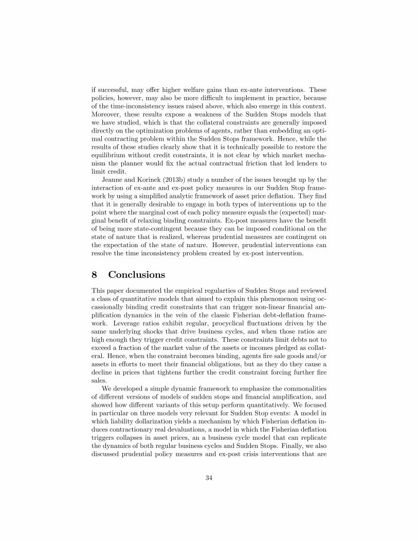
if successful, may offer higher welfare gains than ex-ante interventions. Thesepolicies, however, may also be more diffi cult to implement in practice, becauseof the time-inconsistency issues raised above, which also emerge in this context.Moreover, these results expose a weakness of the Sudden Stops models thatwe have studied, which is that the collateral constraints are generally imposeddirectly on the optimization problems of agents, rather than embedding an opti-mal contracting problem within the Sudden Stops framework. Hence, while theresults of these studies clearly show that it is technically possible to restore theequilibrium without credit constraints, it is not clear by which market mecha-nism the planner would fix the actual contractual friction that led lenders tolimit credit.Jeanne and Korinek (2013b) study a number of the issues brought up by the

interaction of ex-ante and ex-post policy measures in our Sudden Stop frame-work by using a simplified analytic framework of asset price deflation. They findthat it is generally desirable to engage in both types of interventions up to thepoint where the marginal cost of each policy measure equals the (expected) mar-ginal benefit of relaxing binding constraints. Ex-post measures have the benefitof being more state-contingent because they can be imposed conditional on thestate of nature that is realized, whereas prudential measures are contingent onthe expectation of the state of nature. However, prudential interventions canresolve the time inconsistency problem created by ex-post intervention.

8 Conclusions

This paper documented the empirical regularties of Sudden Stops and revieweda class of quantitative models that aimed to explain this phenomenon using oc-cassionally binding credit constraints that can trigger non-linear financial am-plification dynamics in the vein of the classic Fisherian debt-deflation frame-work. Leverage ratios exhibit regular, procyclical fluctuations driven by thesame underlying shocks that drive business cycles, and when those ratios arehigh enough they trigger credit constraints. These constraints limit debts not toexceed a fraction of the market value of the assets or incomes pledged as collat-eral. Hence, when the constraint becomes binding, agents fire sale goods and/orassets in efforts to meet their financial obligations, but as they do they cause adecline in prices that tightens further the credit constraint forcing further firesales.We developed a simple dynamic framework to emphasize the commonalities

of different versions of models of sudden stops and financial amplification, andshowed how different variants of this setup perform quantitatively. We focusedin particular on three models very relevant for Sudden Stop events: A model inwhich liability dollarization yields a mechanism by which Fisherian deflation in-duces contractionary real devaluations, a model in which the Fisherian deflationtriggers collapses in asset prices, an a business cycle model that can replicatethe dynamics of both regular business cycles and Sudden Stops. Finally, we alsodiscussed prudential policy measures and ex-post crisis interventions that are

34

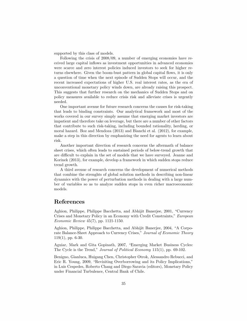
supported by this class of models.Following the crisis of 2008/09, a number of emerging economies have re-

ceived large capital inflows as investment opportunities in advanced economieswere scarce and zero interest policies induced investors to seek for higher re-turns elsewhere. Given the boom-bust pattern in global capital flows, it is onlya question of time when the next episode of Sudden Stops will occur, and therecent increased expectations of higher U.S. real interest rates, as the era ofunconventional monetary policy winds down, are already raising this prospect.This suggests that further research on the mechanics of Sudden Stops and onpolicy measures available to reduce crisis risk and alleviate crises is urgentlyneeded.One important avenue for future research concerns the causes for risk-taking

that leads to binding constraints. Our analytical framework and most of theworks covered in our survey simply assume that emerging market investors areimpatient and therefore take on leverage, but there are a number of other factorsthat contribute to such risk-taking, including bounded rationality, herding, ormoral hazard. Boz and Mendoza (2013) and Bianchi et al. (2012), for example,make a step in this direction by emphasizing the need for agents to learn aboutrisk.Another important direction of research concerns the aftermath of balance

sheet crises, which often leads to sustained periods of below-trend growth thatare diffi cult to explain in the set of models that we have surveyed. Jeanne andKorinek (2013), for example, develop a framework in which sudden stops reducetrend growth.A third avenue of research concerns the development of numerical methods

that combine the strenghts of global solution methods in describing non-lineardynamics with the power of perturbation methods in dealing with a large num-ber of variables so as to analyze sudden stops in even richer macroeconomicmodels.

References

Aghion, Philippe, Philippe Bacchetta, and Abhijit Banerjee, 2001, “CurrencyCrises and Monetary Policy in an Economy with Credit Constraints,”EuropeanEconomic Review 45(7), pp. 1121-1150.

Aghion, Philippe, Philippe Bacchetta, and Abhijit Banerjee, 2004, “A Corpo-rate Balance-Sheet Approach to Currency Crises,”Journal of Economic Theory119(1), pp. 6-30.

Aguiar, Mark and Gita Gopinath, 2007, “Emerging Market Business Cycles:The Cycle is the Trend,”Journal of Political Economy 115(1), pp. 69-102.

Benigno, Gianluca, Huigang Chen, Christopher Otrok, Alessandro Rebucci, andEric R. Young, 2009, “Revisiting Overborrowing and its Policy Implications,”in Luis Cespedes, Roberto Chang and Diego Saravia (editors), Monetary Policyunder Financial Turbulence, Central Bank of Chile.

35

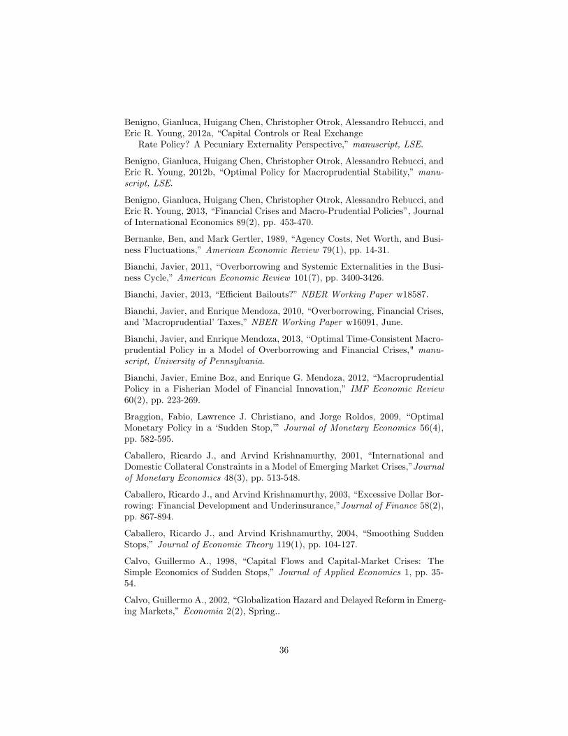
Benigno, Gianluca, Huigang Chen, Christopher Otrok, Alessandro Rebucci, andEric R. Young, 2012a, “Capital Controls or Real ExchangeRate Policy? A Pecuniary Externality Perspective,”manuscript, LSE.

Benigno, Gianluca, Huigang Chen, Christopher Otrok, Alessandro Rebucci, andEric R. Young, 2012b, “Optimal Policy for Macroprudential Stability,”manu-script, LSE.

Benigno, Gianluca, Huigang Chen, Christopher Otrok, Alessandro Rebucci, andEric R. Young, 2013, “Financial Crises and Macro-Prudential Policies”, Journalof International Economics 89(2), pp. 453-470.

Bernanke, Ben, and Mark Gertler, 1989, “Agency Costs, Net Worth, and Busi-ness Fluctuations,”American Economic Review 79(1), pp. 14-31.

Bianchi, Javier, 2011, “Overborrowing and Systemic Externalities in the Busi-ness Cycle,”American Economic Review 101(7), pp. 3400-3426.

Bianchi, Javier, 2013, “Effi cient Bailouts?”NBER Working Paper w18587.

Bianchi, Javier, and Enrique Mendoza, 2010, “Overborrowing, Financial Crises,and ’Macroprudential’Taxes,”NBER Working Paper w16091, June.

Bianchi, Javier, and Enrique Mendoza, 2013, “Optimal Time-Consistent Macro-prudential Policy in a Model of Overborrowing and Financial Crises," manu-script, University of Pennsylvania.

Bianchi, Javier, Emine Boz, and Enrique G. Mendoza, 2012, “MacroprudentialPolicy in a Fisherian Model of Financial Innovation,” IMF Economic Review60(2), pp. 223-269.

Braggion, Fabio, Lawrence J. Christiano, and Jorge Roldos, 2009, “OptimalMonetary Policy in a ‘Sudden Stop,’” Journal of Monetary Economics 56(4),pp. 582-595.

Caballero, Ricardo J., and Arvind Krishnamurthy, 2001, “International andDomestic Collateral Constraints in a Model of Emerging Market Crises,”Journalof Monetary Economics 48(3), pp. 513-548.

Caballero, Ricardo J., and Arvind Krishnamurthy, 2003, “Excessive Dollar Bor-rowing: Financial Development and Underinsurance,”Journal of Finance 58(2),pp. 867-894.

Caballero, Ricardo J., and Arvind Krishnamurthy, 2004, “Smoothing SuddenStops,”Journal of Economic Theory 119(1), pp. 104-127.

Calvo, Guillermo A., 1998, “Capital Flows and Capital-Market Crises: TheSimple Economics of Sudden Stops,” Journal of Applied Economics 1, pp. 35-54.

Calvo, Guillermo A., 2002, “Globalization Hazard and Delayed Reform in Emerg-ing Markets,”Economia 2(2), Spring..

36

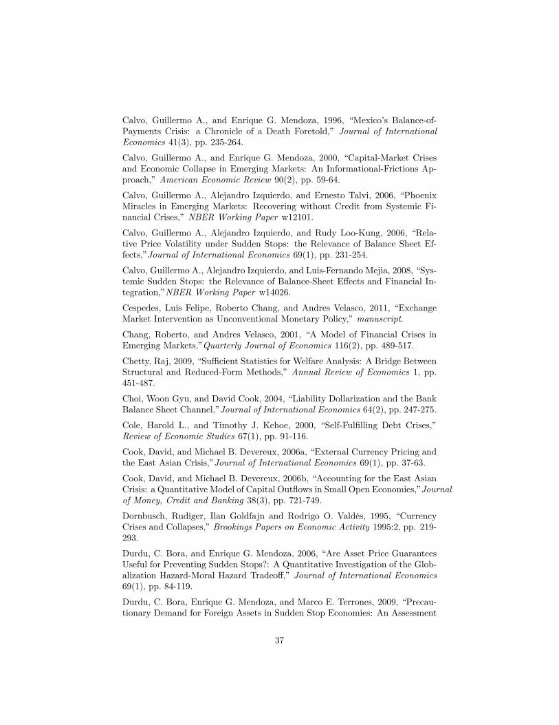
Calvo, Guillermo A., and Enrique G. Mendoza, 1996, “Mexico’s Balance-of-Payments Crisis: a Chronicle of a Death Foretold,” Journal of InternationalEconomics 41(3), pp. 235-264.

Calvo, Guillermo A., and Enrique G. Mendoza, 2000, “Capital-Market Crisesand Economic Collapse in Emerging Markets: An Informational-Frictions Ap-proach,”American Economic Review 90(2), pp. 59-64.

Calvo, Guillermo A., Alejandro Izquierdo, and Ernesto Talvi, 2006, “PhoenixMiracles in Emerging Markets: Recovering without Credit from Systemic Fi-nancial Crises,”NBER Working Paper w12101.

Calvo, Guillermo A., Alejandro Izquierdo, and Rudy Loo-Kung, 2006, “Rela-tive Price Volatility under Sudden Stops: the Relevance of Balance Sheet Ef-fects,”Journal of International Economics 69(1), pp. 231-254.

Calvo, Guillermo A., Alejandro Izquierdo, and Luis-Fernando Mejia, 2008, “Sys-temic Sudden Stops: the Relevance of Balance-Sheet Effects and Financial In-tegration,”NBER Working Paper w14026.

Cespedes, Luis Felipe, Roberto Chang, and Andres Velasco, 2011, “ExchangeMarket Intervention as Unconventional Monetary Policy,”manuscript.

Chang, Roberto, and Andres Velasco, 2001, “A Model of Financial Crises inEmerging Markets,”Quarterly Journal of Economics 116(2), pp. 489-517.

Chetty, Raj, 2009, “Suffi cient Statistics for Welfare Analysis: A Bridge BetweenStructural and Reduced-Form Methods,”Annual Review of Economics 1, pp.451-487.

Choi, Woon Gyu, and David Cook, 2004, “Liability Dollarization and the BankBalance Sheet Channel,”Journal of International Economics 64(2), pp. 247-275.

Cole, Harold L., and Timothy J. Kehoe, 2000, “Self-Fulfilling Debt Crises,”Review of Economic Studies 67(1), pp. 91-116.

Cook, David, and Michael B. Devereux, 2006a, “External Currency Pricing andthe East Asian Crisis,”Journal of International Economics 69(1), pp. 37-63.

Cook, David, and Michael B. Devereux, 2006b, “Accounting for the East AsianCrisis: a Quantitative Model of Capital Outflows in Small Open Economies,”Journalof Money, Credit and Banking 38(3), pp. 721-749.

Dornbusch, Rudiger, Ilan Goldfajn and Rodrigo O. Valdés, 1995, “CurrencyCrises and Collapses,”Brookings Papers on Economic Activity 1995:2, pp. 219-293.

Durdu, C. Bora, and Enrique G. Mendoza, 2006, “Are Asset Price GuaranteesUseful for Preventing Sudden Stops?: A Quantitative Investigation of the Glob-alization Hazard-Moral Hazard Tradeoff,”Journal of International Economics69(1), pp. 84-119.

Durdu, C. Bora, Enrique G. Mendoza, and Marco E. Terrones, 2009, “Precau-tionary Demand for Foreign Assets in Sudden Stop Economies: An Assessment

37

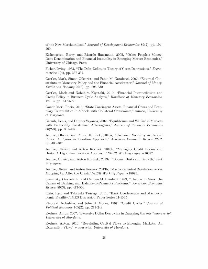
of the New Merchantilism,”Journal of Development Economics 89(2), pp. 194-209.

Eichengreen, Barry, and Ricardo Hausmann, 2005, “Other People’s Money:Debt Denomination and Financial Instability in Emerging Market Economies,”University of Chicago Press.

Fisher, Irving, 1933, “The Debt-Deflation Theory of Great Depressions,”Econo-metrica 1(4), pp. 337-357.

Gertler, Mark, Simon Gilchrist, and Fabio M. Natalucci, 2007, “External Con-straints on Monetary Policy and the Financial Accelerator,”Journal of Money,Credit and Banking 39(2), pp. 295-330.

Gertler, Mark and Nobuhiro Kiyotaki, 2010, “Financial Intermediation andCredit Policy in Business Cycle Analysis,”Handbook of Monetary Economics,Vol. 3, pp. 547-599.

Gondo Mori, Rocio, 2013, “State Contingent Assets, Financial Crises and Pecu-niary Externalities in Models with Collateral Constraints,”mimeo, Universityof Maryland.

Gromb, Denis, and Dimitri Vayanos, 2002, “Equilibrium and Welfare in Marketswith Financially Constrained Arbitrageurs,” Journal of Financial Economics66(2-3), pp. 361-407.

Jeanne, Olivier, and Anton Korinek, 2010a, “Excessive Volatility in CapitalFlows: A Pigouvian Taxation Approach,”American Economic Review P&P,pp. 403-407.

Jeanne, Olivier, and Anton Korinek, 2010b, “Managing Credit Booms andBusts: A Pigouvian Taxation Approach,”NBER Working Paper w16377.

Jeanne, Olivier, and Anton Korinek, 2013a, “Booms, Busts and Growth,”workin progress.

Jeanne, Olivier, and Anton Korinek, 2013b, “Macroprudential Regulation versusMopping Up After the Crash,”NBER Working Paper w18675.

Kaminsky, Graciela L., and Carmen M. Reinhart, 1999, “The Twin Crises: theCauses of Banking and Balance-of-Payments Problems,”American EconomicReview 89(3), pp. 473-500.

Kato, Ryo, and Takayuki Tsuruga, 2011, “Bank Overleverage and Macroeco-nomic Fragility,”IMES Discussion Paper Series 11-E-15.

Kiyotaki, Nobuhiro, and John H. Moore, 1997, “Credit Cycles,” Journal ofPolitical Economy 105(2), pp. 211-248.

Korinek, Anton, 2007, “Excessive Dollar Borrowing in Emerging Markets,”manuscript,University of Maryland.

Korinek, Anton, 2010, “Regulating Capital Flows to Emerging Markets: AnExternality View,”manuscript, University of Maryland.

38

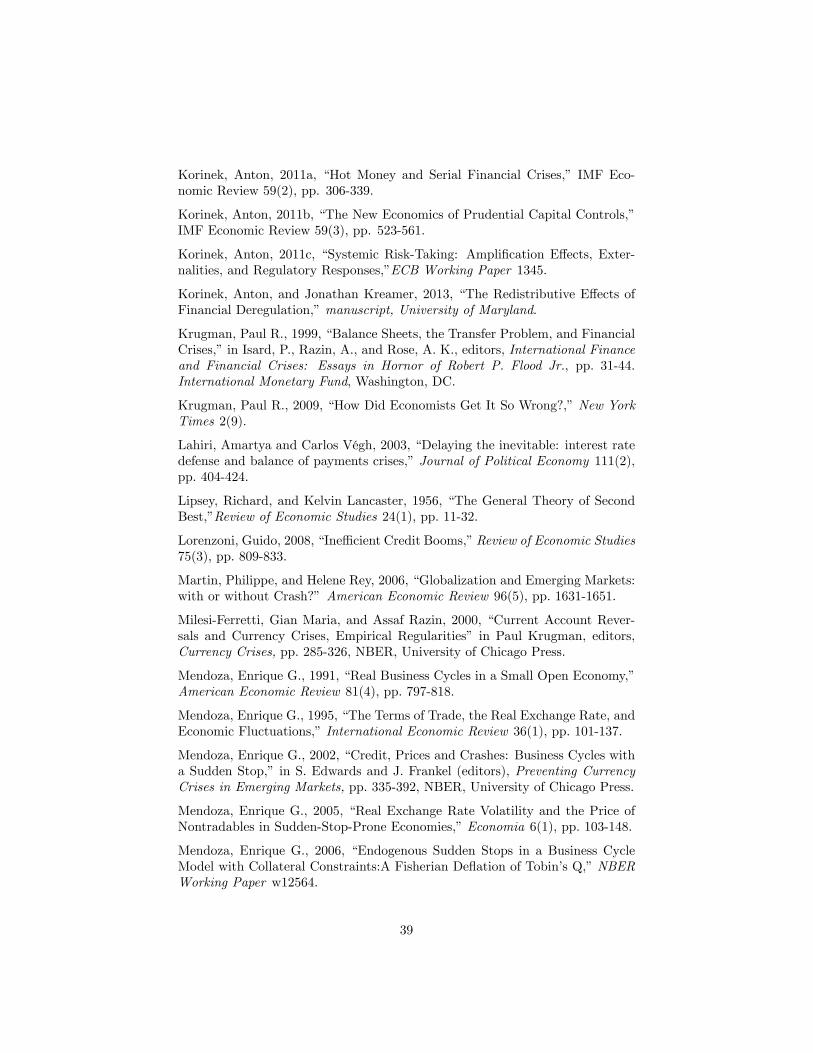
Korinek, Anton, 2011a, “Hot Money and Serial Financial Crises,” IMF Eco-nomic Review 59(2), pp. 306-339.

Korinek, Anton, 2011b, “The New Economics of Prudential Capital Controls,”IMF Economic Review 59(3), pp. 523-561.

Korinek, Anton, 2011c, “Systemic Risk-Taking: Amplification Effects, Exter-nalities, and Regulatory Responses,”ECB Working Paper 1345.

Korinek, Anton, and Jonathan Kreamer, 2013, “The Redistributive Effects ofFinancial Deregulation,”manuscript, University of Maryland.

Krugman, Paul R., 1999, “Balance Sheets, the Transfer Problem, and FinancialCrises,”in Isard, P., Razin, A., and Rose, A. K., editors, International Financeand Financial Crises: Essays in Hornor of Robert P. Flood Jr., pp. 31-44.International Monetary Fund, Washington, DC.

Krugman, Paul R., 2009, “How Did Economists Get It So Wrong?,”New YorkTimes 2(9).

Lahiri, Amartya and Carlos Végh, 2003, “Delaying the inevitable: interest ratedefense and balance of payments crises,”Journal of Political Economy 111(2),pp. 404-424.

Lipsey, Richard, and Kelvin Lancaster, 1956, “The General Theory of SecondBest,”Review of Economic Studies 24(1), pp. 11-32.

Lorenzoni, Guido, 2008, “Ineffi cient Credit Booms,”Review of Economic Studies75(3), pp. 809-833.

Martin, Philippe, and Helene Rey, 2006, “Globalization and Emerging Markets:with or without Crash?”American Economic Review 96(5), pp. 1631-1651.

Milesi-Ferretti, Gian Maria, and Assaf Razin, 2000, “Current Account Rever-sals and Currency Crises, Empirical Regularities” in Paul Krugman, editors,Currency Crises, pp. 285-326, NBER, University of Chicago Press.

Mendoza, Enrique G., 1991, “Real Business Cycles in a Small Open Economy,”American Economic Review 81(4), pp. 797-818.

Mendoza, Enrique G., 1995, “The Terms of Trade, the Real Exchange Rate, andEconomic Fluctuations,”International Economic Review 36(1), pp. 101-137.

Mendoza, Enrique G., 2002, “Credit, Prices and Crashes: Business Cycles witha Sudden Stop,” in S. Edwards and J. Frankel (editors), Preventing CurrencyCrises in Emerging Markets, pp. 335-392, NBER, University of Chicago Press.

Mendoza, Enrique G., 2005, “Real Exchange Rate Volatility and the Price ofNontradables in Sudden-Stop-Prone Economies,”Economia 6(1), pp. 103-148.

Mendoza, Enrique G., 2006, “Endogenous Sudden Stops in a Business CycleModel with Collateral Constraints:A Fisherian Deflation of Tobin’s Q,”NBERWorking Paper w12564.

39

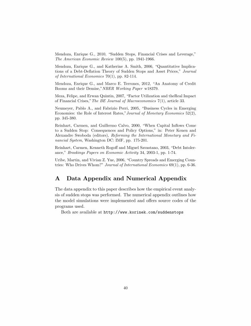
Mendoza, Enrique G., 2010, “Sudden Stops, Financial Crises and Leverage,”The American Economic Review 100(5), pp. 1941-1966.

Mendoza, Enrique G., and Katherine A. Smith, 2006, “Quantitative Implica-tions of a Debt-Deflation Theory of Sudden Stops and Asset Prices,” Journalof International Economics 70(1), pp. 82-114.

Mendoza, Enrique G., and Marco E. Terrones, 2012, “An Anatomy of CreditBooms and their Demise,”NBER Working Paper w18379.

Meza, Felipe, and Erwan Quintin, 2007, “Factor Utilization and theReal Impactof Financial Crises,”The BE Journal of Macroeconomics 7(1), article 33.

Neumeyer, Pablo A., and Fabrizio Perri, 2005, “Business Cycles in EmergingEconomies: the Role of Interest Rates,”Journal of Monetary Economics 52(2),pp. 345-380.

Reinhart, Carmen, and Guillermo Calvo, 2000, “When Capital Inflows Cometo a Sudden Stop: Consequences and Policy Options,” in: Peter Kenen andAlexandre Swoboda (editors), Reforming the International Monetary and Fi-nancial System, Washington DC: IMF, pp. 175-201.

Reinhart, Carmen, Kenneth Rogoff and Miguel Savastano, 2003, “Debt Intoler-ance,”Brookings Papers on Economic Activity 34, 2003-1, pp. 1-74.

Uribe, Martin, and Vivian Z. Yue, 2006, “Country Spreads and Emerging Coun-tries: Who Drives Whom?”Journal of International Economics 69(1), pp. 6-36.

A Data Appendix and Numerical Appendix

The data appendix to this paper describes how the empirical event analy-sis of sudden stops was performed. The numerical appendix outlines howthe model simulations were implemented and offers source codes of theprograms used.Both are available at http://www.korinek.com/suddenstops

40