Embed Size (px)
Citation preview

Subsea motor drives with long subsea cable
Sergey Klyapovskiy
Master of Science in Electric Power Engineering
Supervisor: Arne Nysveen, ELKRAFTCo-supervisor: Kristen Jomås, SmartMotorAS
Department of Electric Power Engineering
Submission date: June 2014
Norwegian University of Science and Technology


NORGES TEKNISK-NATURVITENSKAPELIGE UNIVERSITET
NTNU
M A S T E R O P P G A V E
Kandidatens navn :Sergey Klyapovskiy
Fag : ELKRAFTTEKNIKK
Oppgavens tittel (norsk) : Undervanns motordrift med lang kabel
Oppgavens tittel (engelsk) : Subsea motor drives with long subsea cable
Oppgavens tekst:Motors driving subsea devices in oil and gas production, such as pumps and compressors, may be operated via long step outs. Today there is the trend to try permanent magnet (PM) motors instead of traditional induction motors. However, application of PM motors brings along different challenges, for example starting of the driven unit in an open loop motor control.
In this work focus is on dynamic modelling and simulation of the subsea PM motor supplied by a long subsea cable. Based on the results from the student project fall semester 2013, the ability to obtain a safe start-up and adjustment to load changes are two most critical issues for further study.
The overall objective of the study in this project work is to study these critical aspects of a subsea PM motor drive with a long subsea cable and compare its performance with an induction motor drive.
More specifically the work shall focus on:
Development and testing of SimuLink models for dynamic analysis of PM subsea motordrive
Study different start-up procedures and response to sudden load changes
Study the influence of cable length and a subsea transformer
Compare the performance of PM drives with induction motor drives
Further details to be discussed with the supervisors during the project period.


iii
Preface
This thesis is submitted in partial fulfillment of the requirements for the degree of Master
of Science in Electric Power Engineering. The work has been done during the spring semester
2014 at the Department of Electric Power Engineering at Norwegian University of Science and
Technology under cooperation of NTNU and SmartMotor AS. The thesis based on previous
specialization project “Subsea PM motor drives with long step out distance” written by the same
student in the fall 2013.
I would like to express my gratitude to my supervisors Professor Arne Nysveen at NTNU
and Kristen Jomås at SmartMotor AS for their guidance and valuable feedback.
Special thanks to Alexey Matveev from SmartMotor AS for his comments and help
during the master thesis discussions.
Finally, I would like to thank my family for the support they gave me during that period.
Norwegian University of Science and Technology
Trondheim 16.06.2014
Sergey Klyapovskiy

iv
Abstract
Oil and gas are extracted from the fields by the pumps, which are driven by the electrical
motors. With the tendency to increase the distance between the platform and the subsea field,
where the motor is installed, the problem of machine start-up becomes more and more urgent.
Two biggest problems during the motor start-up are the need to limit the maximum
currents through frequency converter and to avoid transformer saturation at the same time. In
special cases, due to the increased impedance of the longer cables, there will be no possibility to
start-up the motor at all. The oversizing of the system components is required in order to
withstand the high stresses at starting.
Induction machines were the main choice for the subsea applications since the beginning
of the subsea era, but recently they become replaced by the permanent-magnet synchronous
machine. Due to their inherited advantages, the use of permanent-magnet motors allows to
achieve lower losses and higher efficiency of the system. Both types of machines are analyzed in
this master thesis.
The system for the power supply of the electric motor is designed and simulated in
Matlab/Simulink. Two different topologies are used in simulations: topology with one step-up
transformer and topology with an additional subsea transformer. The conventional method of
motor start-up is tested in order to show the challenges that can be encountered.
Both IM and PM motors are able to start with the designed system. The results show the
superior performance of the systems with PM motor in terms of the transformer flux and system
currents. The extension of the step out distance brings corresponding increase in the transformer
flux, which can reach magnitude of 3 pu for the system with PM machine and 50km cable.
A transformer bypass is a new starting method, suggested by SmartMotor AS. It should
allow to fully eliminate transformer saturation problem, thus making the motor starting easier.
The simulation results indicate that system with implemented transformer bypass can be used for
starting of the motors. The usage of bypass in one transformer topology allows to reduce the
transformer fluxes to the rated values and avoid oversizing. Additional challenges arise during
implementation of the bypass into the system with subsea transformer. The impossibility of
bypassing that transformer and necessity of early reconnection results in the higher than nominal
fluxes in transformer. The oversizing of the core is thus still required, but at a lower degree in
comparison with conventional starting methods for the same system.
Keywords: PM, IM, saturation, transformer bypass, frequency converter.
Table of contents 1. Introduction ............................................................................................................................................... 1
1.1. Problem definition .............................................................................................................................. 1
1.2. Scope of work ........................................................................................................................................ 2
2. System description .................................................................................................................................. 4
2.1. Topside system and frequency converter ................................................................................. 4
2.2. Transformer .......................................................................................................................................... 6
2.3. Subsea cable .......................................................................................................................................... 8
2.4. Subsea motor ..................................................................................................................................... 10
2.4.1 Induction motor ............................................................................................................................ 10
2.4.2 Permanent magnet synchronous motor ............................................................................. 13
2.5. PMSM vs IM technology ................................................................................................................. 16
3. Equivalent impedance calculation ................................................................................................. 17
3.1. Transmission system ...................................................................................................................... 17
3.2. Per-unit system ................................................................................................................................. 18
3.3. Thevenin equivalent ........................................................................................................................ 19
3.4. Results .................................................................................................................................................. 23
4. Start-up procedure ............................................................................................................................... 25
4.1. Motor start-up ................................................................................................................................... 25
4.2. Transformer saturation ................................................................................................................. 26
4.3. Start-up limitations ......................................................................................................................... 29
4.4. Inrush currents and transformer bypass ................................................................................ 31
5. Simulink models .................................................................................................................................... 35
5.1. Power source model ........................................................................................................................ 35
5.2. Load model ......................................................................................................................................... 39
6. Simulation results ................................................................................................................................. 42
6.1. Case 1a – Start-up of PM with step-up transformer ........................................................... 42
6.2. Case 1b – Start-up of IM with step-up transformer ............................................................ 46
6.3. Case 2a – Start-up of PM with two transformers ................................................................. 48
6.4. Case 2b – Start-up of IM with two transformers .................................................................. 52
6.5. Case 3a – PM system with step-up transformer and bypass ........................................... 53
6.6. Case 3b – IM system with step-up transformer and bypass ............................................ 56
6.7. Case 4a – PM system with two transformer and bypass ................................................... 59
6.8. Case 4b – IM system with two transformer and bypass ................................................... 61

6.9. PM vs IM ............................................................................................................................................... 62
7. Conclusion ............................................................................................................................................... 64
8. Future work ............................................................................................................................................ 66
References ............................................................................................................................................................ 67
Appendix A ....................................................................................................................................................... 69
Appendix B ....................................................................................................................................................... 72
Appendix C ....................................................................................................................................................... 76
1
1. Introduction
This chapter describes the problems addressed in the master thesis, presents the scope of
work and used methodology.
1.1. Problem definition
The subsea oil and gas industry has grown rapidly in the last several decades. New
deposits were discovered and started to exploit. The attempts of reducing the cost of the field
development led to the idea of tying new fields to the already existed platforms, thus
substantially reducing expenses. The production equipment for the fields is installed on the
seabed and gets the required electrical power from the platform. But despite of the obvious
advantages of such approach, new problems arise together with increasing of the distance
between the production field and offshore platform it is connected to [1].
Subsea pumps driven by the electrical motors are the main part of the production
equipment. So called “stiction torque” imposed by the static friction in the machine should be
overcome in order to start-up the motor and the pump. In the worst cases the stiction is equal to
30% of the nominal torque. The motor starting currents can reach magnitude of 5-7 times of the
nominal values. Since such high currents will impose a great stress upon system components,
especially the power electronic devices, certain measures should be applied to limit them. In
present systems the power from the platform goes through a step-up transformer. The magnetic
material of its core can be driven into the saturation by applying too much voltage at low
frequency. It will bring unwanted nonlinearity into the system and therefore saturation of the
transformer should be avoided. To extend the allowable cable lengths the additional subsea step-
down transformer can be added to the system. This gives the opportunity to reduce the size of the
cable and limit the voltage drop.
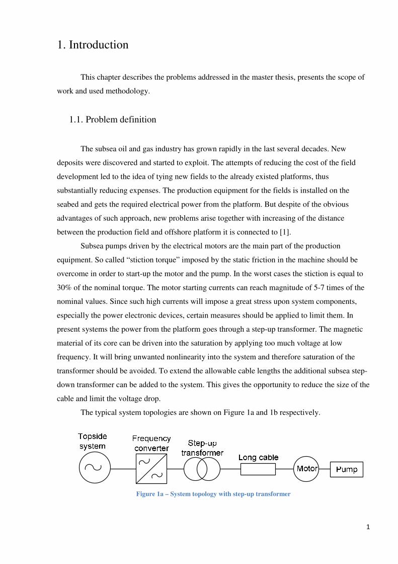
The typical system topologies are shown on Figure 1a and 1b respectively.
Figure 1a – System topology with step-up transformer
2
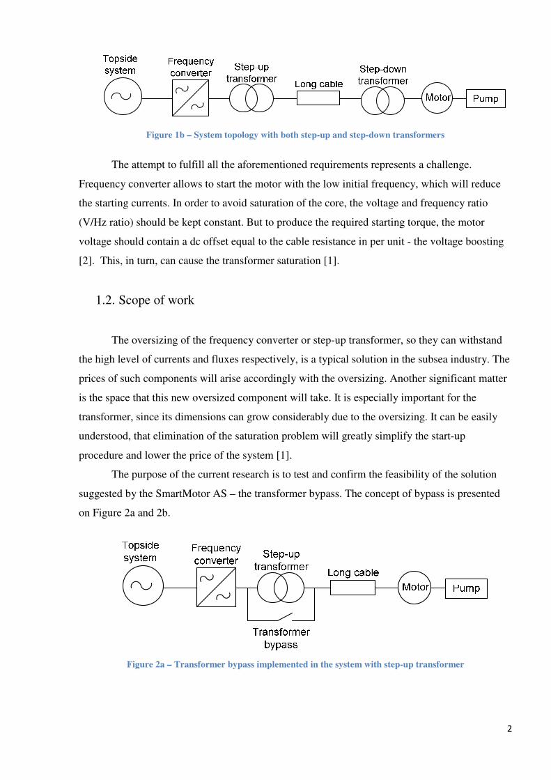
Figure 1b – System topology with both step-up and step-down transformers
The attempt to fulfill all the aforementioned requirements represents a challenge.
Frequency converter allows to start the motor with the low initial frequency, which will reduce
the starting currents. In order to avoid saturation of the core, the voltage and frequency ratio
(V/Hz ratio) should be kept constant. But to produce the required starting torque, the motor
voltage should contain a dc offset equal to the cable resistance in per unit - the voltage boosting
[2]. This, in turn, can cause the transformer saturation [1].
1.2. Scope of work
The oversizing of the frequency converter or step-up transformer, so they can withstand
the high level of currents and fluxes respectively, is a typical solution in the subsea industry. The
prices of such components will arise accordingly with the oversizing. Another significant matter
is the space that this new oversized component will take. It is especially important for the
transformer, since its dimensions can grow considerably due to the oversizing. It can be easily
understood, that elimination of the saturation problem will greatly simplify the start-up
procedure and lower the price of the system [1].
The purpose of the current research is to test and confirm the feasibility of the solution
suggested by the SmartMotor AS – the transformer bypass. The concept of bypass is presented
on Figure 2a and 2b.
Figure 2a – Transformer bypass implemented in the system with step-up transformer
3
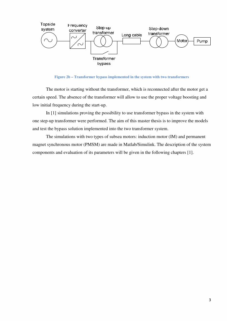
Figure 2b – Transformer bypass implemented in the system with two transformers
The motor is starting without the transformer, which is reconnected after the motor get a
certain speed. The absence of the transformer will allow to use the proper voltage boosting and
low initial frequency during the start-up.
In [1] simulations proving the possibility to use transformer bypass in the system with
one step-up transformer were performed. The aim of this master thesis is to improve the models
and test the bypass solution implemented into the two transformer system.
The simulations with two types of subsea motors: induction motor (IM) and permanent
magnet synchronous motor (PMSM) are made in Matlab/Simulink. The description of the system
components and evaluation of its parameters will be given in the following chapters [1].
4
2. System description
In the current project the motor start-up procedure is analyzed for two main topologies:
with and without subsea transformer. The presence of subsea (or step-down) transformer allows
to significantly increase the possible cable length (up to hundreds of km). The chapter deals with
the description of all components the aforementioned systems comprised of. The per-phase
equivalent circuits that will be used in the further analysis are given and discussed.
2.1. Topside system and frequency converter
In the subsea power systems the term “topside” refers to the components that are not
submerged in the seawater and generally located on the oil platforms. The electric power comes
either from systems own generators or through the cables connected to the power station
onshore. The topside system in this project is assumed to be an infinite bus with the capability of
providing stable and reliable voltage regardless of the motor’s operation conditions.
The voltage and even the frequency of the topside system can be different from the ones
required by the rest of the equipment. This creates the need for the device that can match the
input power with the output. Another desirable feature is the ability of changing the voltage and
frequency in the quick, accurate and precise manner on the all range from initial to the rated
values. All these requirements are fulfilled by using frequency converter (FC) at the topside
system’s output.
FC is the power electronic device, which produces the output voltage of varying
amplitude and frequency. By changing these two parameters the AC motor speed and torque can
be easily controlled, which is in turn beneficial for the pump operation. With the conventional
system, the pump will consume the rated power and produce rated flow rate, even if it is not
needed. To overcome this problem throttling operation was used before. The drawback of that
method is the drop in the efficiency. With FC the voltage, frequency and power supplied to
motor are adjusted according to the real demand.
5
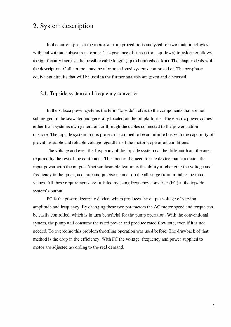
Figure 3 – Frequency converter
FC consists of the AC/DC and DC/AC power electronics converters connected through
the DC-link and are shown on Figure 3 [3]. Usually the FC allows only the unidirectional
transfer of power from the power source to the load, though nowadays trend is to allow to feed
the excessive power obtained during the motor braking back to the grid. Wide variety of
semiconductor devices can be used in the FC configuration shown on Figure 3: power diodes,
thyristors, MOSFETs and IGBTs. Each of them has their best operating area in regards with
applied voltage and power. For the designed system the insulated-gate bipolar transistors
(IGBTs) should be chosen for the FC to handle the high power demand from the AC motor.
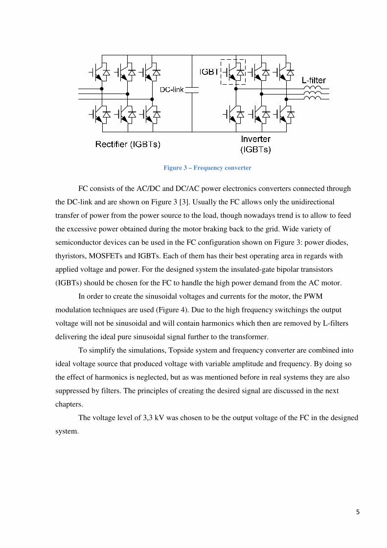
In order to create the sinusoidal voltages and currents for the motor, the PWM
modulation techniques are used (Figure 4). Due to the high frequency switchings the output
voltage will not be sinusoidal and will contain harmonics which then are removed by L-filters
delivering the ideal pure sinusoidal signal further to the transformer.
To simplify the simulations, Topside system and frequency converter are combined into
ideal voltage source that produced voltage with variable amplitude and frequency. By doing so
the effect of harmonics is neglected, but as was mentioned before in real systems they are also
suppressed by filters. The principles of creating the desired signal are discussed in the next
chapters.
The voltage level of 3,3 kV was chosen to be the output voltage of the FC in the designed
system.
6
Figure 4 – PWM with triangular waveform. a) timing waveforms, b)-d) switch voltages,
e) output line voltage [3]
2.2. Transformer
One of the main tasks during design of power systems is to minimize the losses that will
occur during the power transfer from generation source to the end equipment. Since such losses
are proportional to the square of the current, the most common solution is to increase the voltage
level, thus lowering the current magnitude. This is done by the power transformer – an electrical
device which transforms AC voltage of one magnitude to the AC voltage of another magnitude.
The energy is transferred by the inductive coupling of its winding circuits.
Since the FC output voltage is usually smaller than that required by the machine, step-up
transformer is installed. If there is a significant distance between the platform and the motor and
the machine is designed for high power and requires a large current, the size of the cable and
7
transmission losses becomes too high. In this case the combination of step-up and step-down
transformers is applied. The step-down transformer in this configuration is put on the seabed and
thus can be also called “subsea transformer”. There are no principal differences between step-up
and subsea transformer operation.
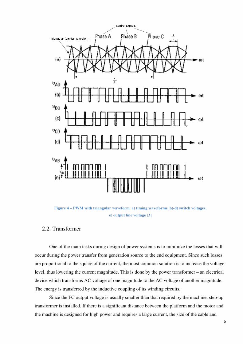
The equivalent circuit of the transformer is shown on Figure 5 [4]. Parameters of the
secondary side are referred to the primary side through the coefficients [1].
Figure 5 – Transformer equivalent circuit referred to the primary side
where
������′�– primary and referred secondary side voltages,
����′�– primary and referred secondary side currents,
, �, – no-load current, magnetizing current and eddy current respectively,
��, ������′�, �′�– primary and referred secondary side resistances and reactances,
� �������– magnetizing resistance and reactance,
��– electromotive force (emf).
The power transformer consists of the core made of the magnetic material with several
windings wound on it. To access the amount of the magnetic field passing through the core the
term “magnetic flux” is used. The flux in the transformer is lagging the emf by 90 degrees and its
maximum value can be found through the Equation 17:
�� = 4,44��1���
Equation 1
where
��– number of windings on the primary side,
Ф���– maximum value of the flux in the transformer.
It is seen from Equation 17, that in order to keep the constant flux in the transformer, the
constant E/f ratio should be maintained. The method is widely used for the system start-up.
8
For the analyzed system it was decided to use transformer 3,3/6,6 kV for the case with
only one step-up transformer (case 1) and two transformers: 3,3/30 kV and 30/6,6 kV for the
system with 30 and 50 km cable lengths (case 2).
The parameters of the chosen equipment are shown in Table 1. The transformer apparent
power ST was chosen based on the preliminary motor active and reactive power estimations and
losses in the transmission components. The values for resistance and reactance are given in %,
the real values can be easily obtained using per-unit system.
Table 1 – Transformer parameters
Function Apparent power,
ST, [MVA]
Primary voltage,
U1, [kV] rms
Secondary voltage,
U2, [kV] rms
Resistance,
[%]
Reactance,
[%]
Step-up (case 1) 8 3,3 6,6 1 5
Step-up (case 2) 8 3,3 30 1 5
Subsea (case 2) 8 30 6,6 1 5
2.3. Subsea cable
The choice of the suitable cable model is defined by its length. Lengths in the range from
5 to 50 km are investigated in the current project. The simplest short cable model is not taken
into account the charging capacities distributed along the cable. These capacitances become
significantly large with the increase of the cable length and so cannot be omitted. Due to
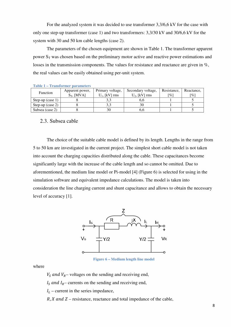
aforementioned, the medium line model or Pi-model [4] (Figure 6) is selected for using in the
simulation software and equivalent impedance calculations. The model is taken into
consideration the line charging current and shunt capacitance and allows to obtain the necessary
level of accuracy [1].
Figure 6 – Medium length line model
where
�������– voltages on the sending and receiving end,
�����– currents on the sending and receiving end,
�– current in the series impedance,
�, �����– resistance, reactance and total impedance of the cable,
9
�– admittance, in this model � = �� !" ∗ $%�&'ℎ.
The medium length line model is described by two equations:
�� = )1 + ��2 , ∗ �� + � ∗ �
Equation 2
� = � )1 + ��4 , ∗ �� + )1 + ��2 , ∗ �
Equation 3
To choose the proper size of the cable, the current (IMotor) needed for the subsea motor is
calculated by the following equation:
-./.0 = 1-./.0√34��-./.0 ∗ 5678
Equation 4
where
1-./.0– motor active power,
4��-./.0– line-to-line terminal voltage,
5678– power factor (due to the lack of data use typical value 0,8).
IMotor = 546,7 [A], rms from Equation 4, which gives ICable = 546,7 [A], rms for case 1 and
ICable = 120,3 [A], rms for case 2 with subsea transformer. From [5] and [6] choose three-core
XLPE cables with copper conductors. Cable parameters are given in Table 2.
Table 2 – Subsea cable parameters
Length Cross-section,
[mm2]
Current, [A],
rms
Resistance,
[Ohm/km]
Inductance,
[mH/km]
Capacitance,
[uF/km]
5 km 400 590 0,0470 0,31 0,59
30 and 50 km 95 300 0,193 0,44 0,18
In some cases it can be beneficial to install the cable with larger cross-section area than
needed due to the current requirements and reduce the voltage drop in the system. But the final
decision whether to increase the cable or not should be done only after conducting thorough
technical and economic analyses.
10
2.4. Subsea motor
There are two types of motors, which operation will be analyzed in the current project:
Induction Motor and Permanent Magnet Synchronous Motor. While IM is the proven solution
which was used from the earliest subsea applications, subsea PMSM is a new emerging solution
with higher efficiency and higher rotational speed [7].
2.4.1 Induction motor
The induction motor (IM) is an AC electric motor and consists of the stationary (stator)
and rotating (rotor) parts. The stator of IM has three-phase windings, while the rotor can be made
either with windings or with conductive bars connected by the shorting rings at both ends. The
latter rotor construction is called the squirrel-cage and is chosen for the motor simulation.
By applying the AC voltage to the stator windings, the stator current is starting to flow.
As a result, the magnetic field is created in the stator. This magnetic field is rotating with the
synchronous speed �9:; and according to the Lenz law inducing the emf in the rotor bars, when
the stator flux “cuts” them. The rotor current caused by the induced emf will then produce the
force and the torque in the machine [1].
Synchronous speed is defined by the Equation 5:
�9:; = 120�=
Equation 5
where
�– frequency of the network, �= 100 Hz,
=– number of poles.
The rotor cannot rotate with the same synchronous speed as the stator magnetic field.
This is due to the fact, that if the rotor will have that speed, no flux will cross the rotor bars and
there will be no induced rotor currents. The difference between the actual rotor and synchronous
speed is called “the slip”. At the first moment of machine startup, the slip equals to 1 (or 100%)
and then is reducing while the motor approaching the nominal operation mode. The typical
values of the slip are in the range of 0,5 to 5%.
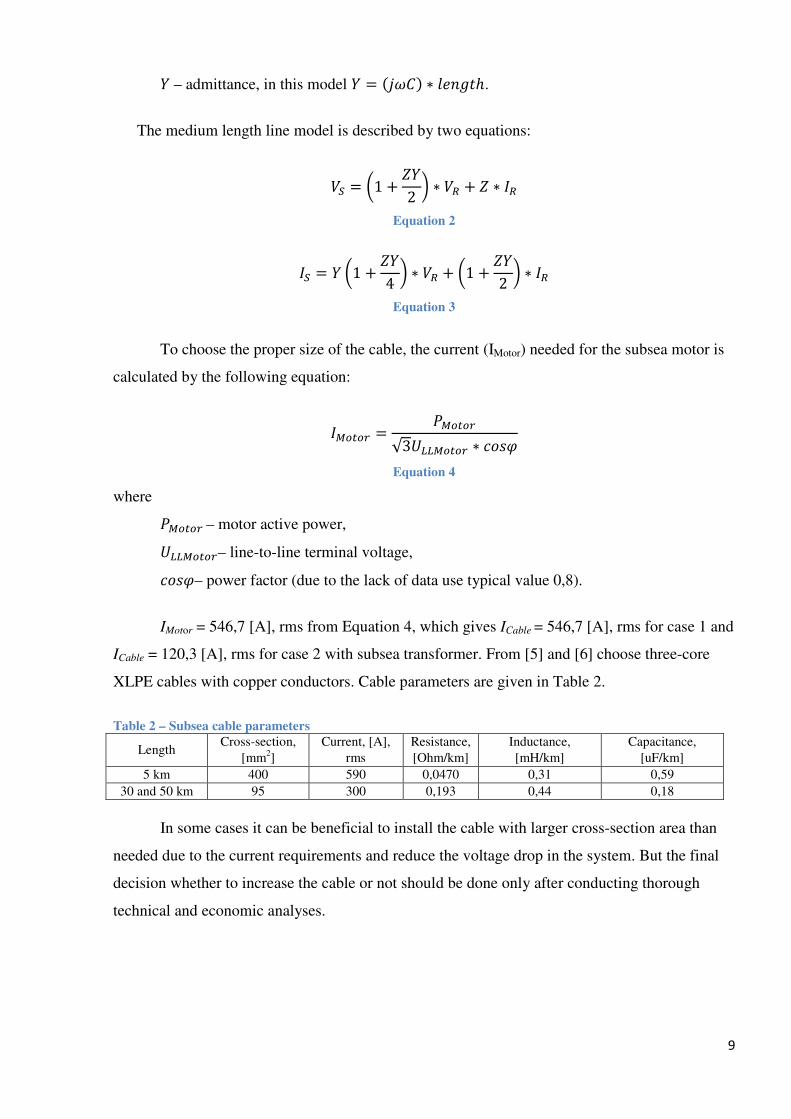
The equivalent circuit of the IM is similar to the transformer circuit on Figure 5.
11
Figure 7 – Equivalent circuit of the IM
where
�9– stator voltage,
9���0– stator and rotor currents,
�9, �9����0 , �0– stator and rotor resistance and reactance,
��– magnetizing reactance,
7– slip.
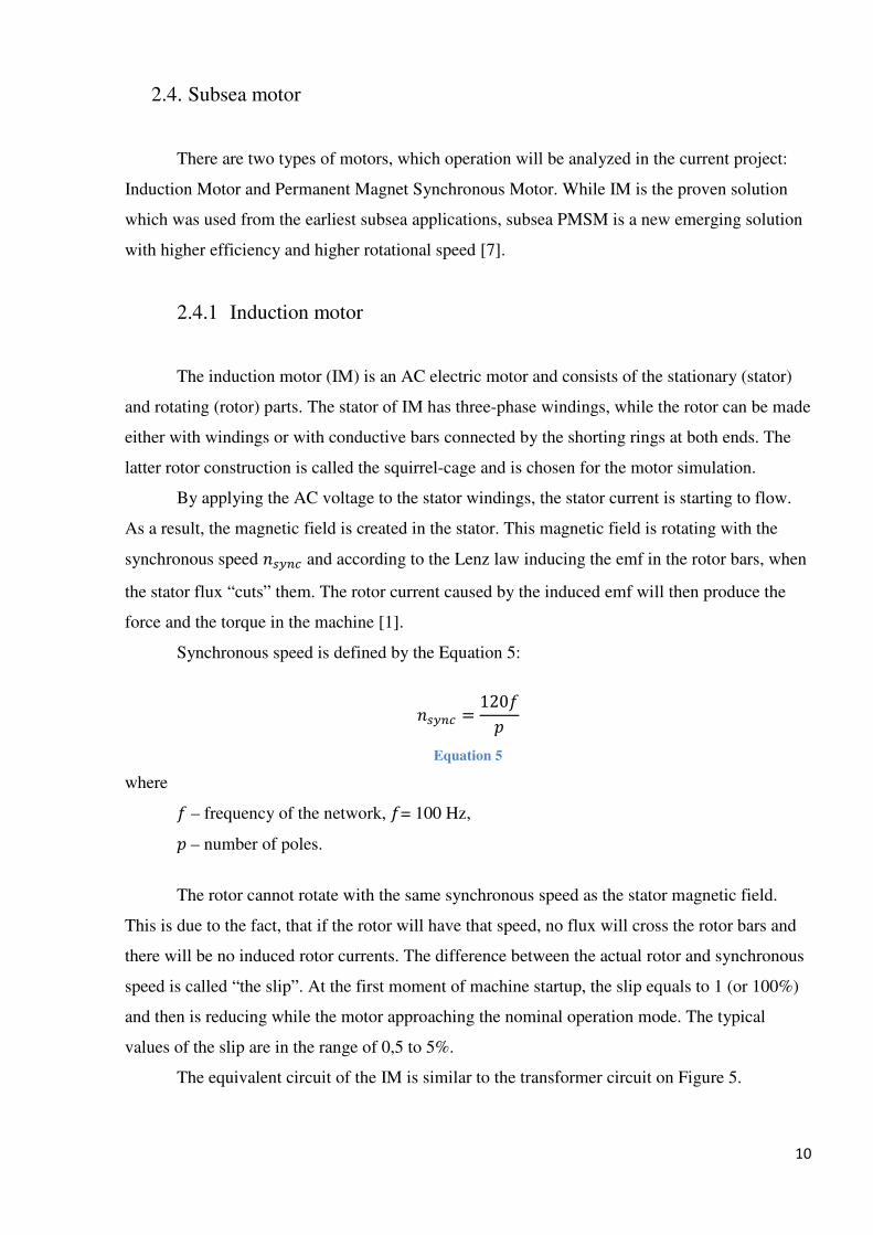
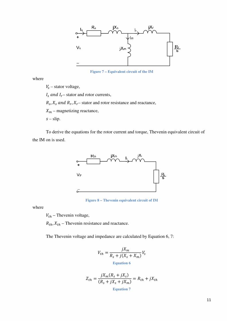
To derive the equations for the rotor current and torque, Thevenin equivalent circuit of
the IM on is used.
Figure 8 – Thevenin equivalent circuit of IM
where
�/>– Thevenin voltage,
�/>, �/>– Thevenin resistance and reactance.
The Thevenin voltage and impedance are calculated by Equation 6, 7:
�/> = ����9 + ���9 + ��"�9 Equation 6
�/> = �����9 + ��9"��9 + ��9 + ���" = �/> + ��/>
Equation 7
12
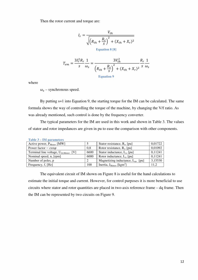
Then the rotor current and torque are:
0 = �/>?@�/> + �07 A� + ��/> + �0"�
Equation 8 [8]
BC� = 30��07 1 9 = 3�/>�@�/> + �07 A� + ��/> + �0"�
�07 1 9 Equation 9
where
9– synchronous speed.
By putting s=1 into Equation 9, the starting torque for the IM can be calculated. The same
formula shows the way of controlling the torque of the machine, by changing the V/f ratio. As
was already mentioned, such control is done by the frequency converter.
The typical parameters for the IM are used in this work and shown in Table 3. The values
of stator and rotor impedances are given in pu to ease the comparison with other components.
Table 3 – IM parameters
Active power, PMotor, [MW] 5 Stator resistance, Rs, [pu] 0,01722
Power factor−5678 0,8 Rotor resistance, Rr, [pu] 0,01092
Terminal line voltage, ULLMotor, [V] 6600 Stator inductance, Ls, [pu] 0,11241
Nominal speed, n, [rpm] 6000 Rotor inductance, Lr, [pu] 0,11241
Number of poles, p 2 Magnetizing inductance, Lm, [pu] 3,15530
Frequency, f, [Hz] 100 Inertia, JMotor, [kgm2] 11,2
The equivalent circuit of IM shown on Figure 8 is useful for the hand calculations to
estimate the initial torque and current. However, for control purposes it is more beneficial to use
circuits where stator and rotor quantities are placed in two-axis reference frame – dq frame. Then
the IM can be represented by two circuits on Figure 9.
13
Ψ
Ψ
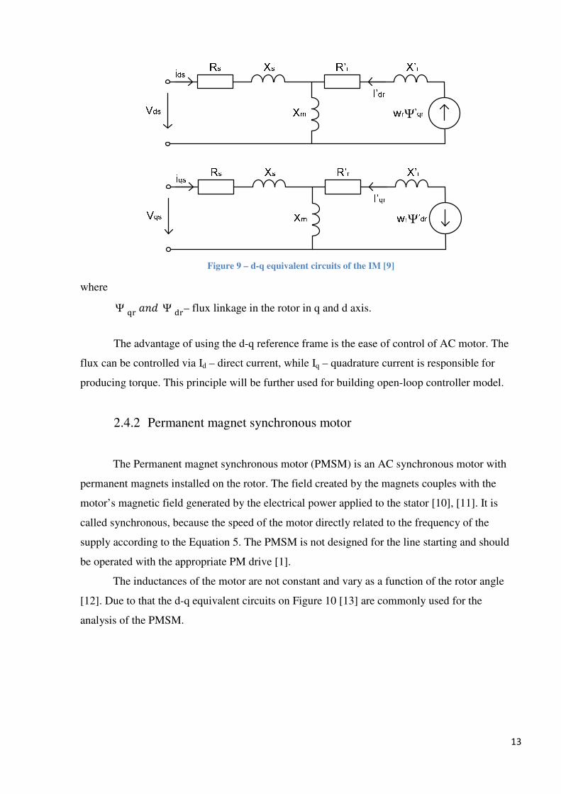
Figure 9 – d-q equivalent circuits of the IM [9]
where
Ψ EF���Ψ GF– flux linkage in the rotor in q and d axis.
The advantage of using the d-q reference frame is the ease of control of AC motor. The
flux can be controlled via Id – direct current, while Iq – quadrature current is responsible for
producing torque. This principle will be further used for building open-loop controller model.
2.4.2 Permanent magnet synchronous motor
The Permanent magnet synchronous motor (PMSM) is an AC synchronous motor with
permanent magnets installed on the rotor. The field created by the magnets couples with the
motor’s magnetic field generated by the electrical power applied to the stator [10], [11]. It is
called synchronous, because the speed of the motor directly related to the frequency of the
supply according to the Equation 5. The PMSM is not designed for the line starting and should
be operated with the appropriate PM drive [1].
The inductances of the motor are not constant and vary as a function of the rotor angle
[12]. Due to that the d-q equivalent circuits on Figure 10 [13] are commonly used for the
analysis of the PMSM.
14
Ψ
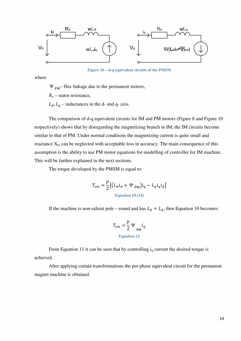
Figure 10 – d-q equivalent circuits of the PMSM
where
Ψ HI– flux linkage due to the permanent motors,
�9– stator resistance,
JK , JL– inductances in the d- and q- axis.
The comparison of d-q equivalent circuits for IM and PM motors (Figure 8 and Figure 10
respectively) shows that by disregarding the magnetizing branch in IM, the IM circuits become
similar to that of PM. Under normal conditions the magnetizing current is quite small and
reactance Xm can be neglected with acceptable loss in accuracy. The main consequence of this
assumption is the ability to use PM motor equations for modelling of controller for IM machine.
This will be further explained in the next sections.
The torque developed by the PMSM is equal to:
BC� = =2 MNJKOK + Ψ HIPOL − JLOLOKQ Equation 10 [14]
If the machine is non-salient pole – round and has JK = JL, then Equation 10 becomes:
BC� = =2 Ψ HIOL
Equation 11
From Equation 11 it can be seen that by controlling iq current the desired torque is
achieved.
After applying certain transformations the per-phase equivalent circuit for the permanent
magnet machine is obtained.
15
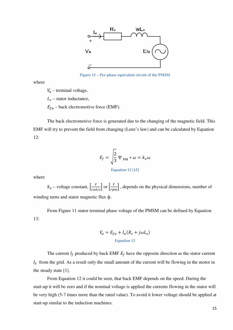
Figure 11 – Per-phase equivalent circuit of the PMSM
where
��– terminal voltage,
J9– stator inductance,
�R�– back electromotive force (EMF).
The back electromotive force is generated due to the changing of the magnetic field. This
EMF will try to prevent the field from changing (Lenz’s law) and can be calculated by Equation
12:
�R = S23 Ψ HI ∗ = TC
Equation 12 [15]
where
TC– voltage constant, U V0�K/9X or U V0Y�X, depends on the physical dimensions, number of
winding turns and stator magnetic flux ф.
From Figure 11 stator terminal phase voltage of the PMSM can be defined by Equation
13:
�� = �R� + ���9 + � J9" Equation 13
The current R produced by back EMF �R have the opposite direction as the stator current
� from the grid. As a result only the small amount of the current will be flowing in the motor in
the steady state [1].
From Equation 12 it could be seen, that back EMF depends on the speed. During the
start-up it will be zero and if the nominal voltage is applied the currents flowing in the stator will
be very high (5-7 times more than the rated value). To avoid it lower voltage should be applied at
start-up similar to the induction machines.
16
In some cases, the machine can have too high induced voltage (back EMF) and cannot
reach nominal speed without flux weaking.
In opposition to IM, which can start with certain initial frequency (up to 10 Hz), the
starting frequency for PM should be zero. This is due to the magnets on PM machine rotor. If the
initial frequency is too high the magnets will not be able to follow the magnetic field and motor
will start vibrating instead.
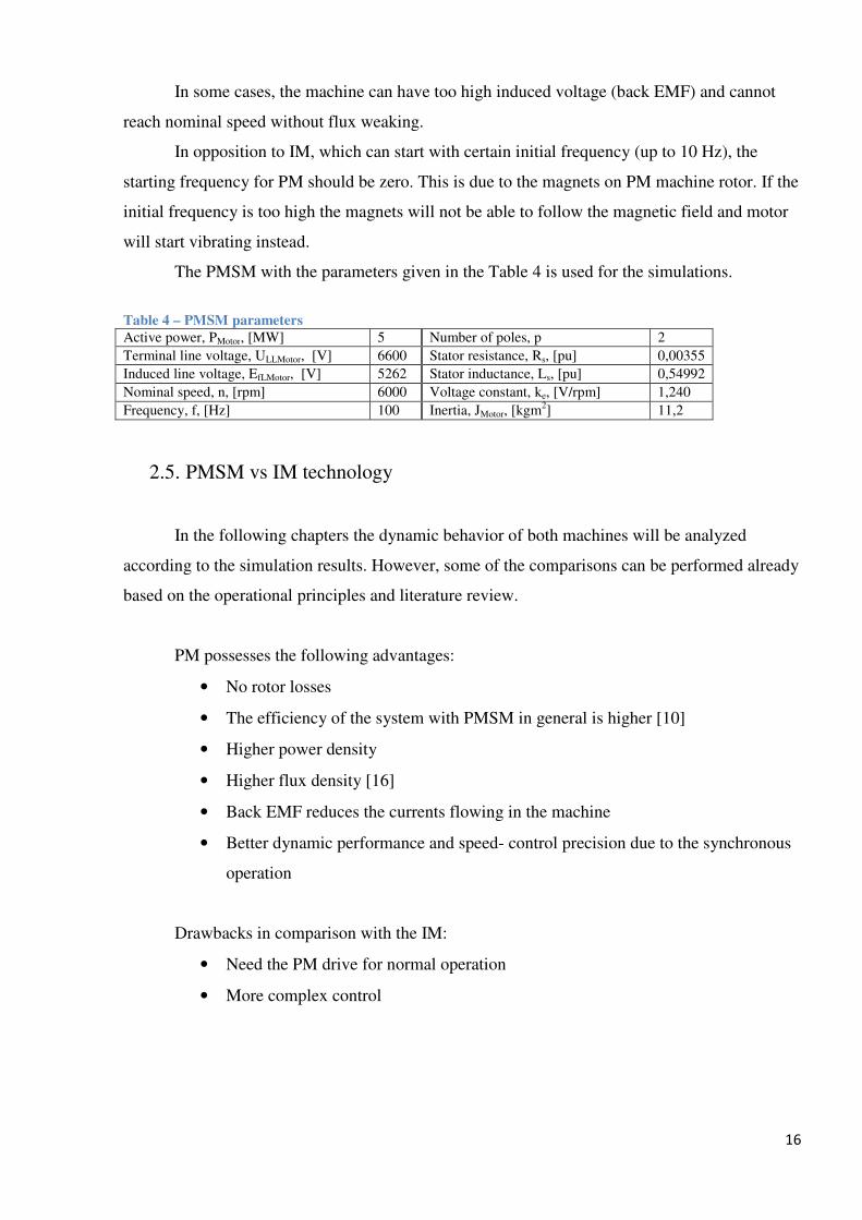
The PMSM with the parameters given in the Table 4 is used for the simulations.
Table 4 – PMSM parameters
Active power, PMotor, [MW] 5 Number of poles, p 2
Terminal line voltage, ULLMotor, [V] 6600 Stator resistance, Rs, [pu] 0,00355
Induced line voltage, EfLMotor, [V] 5262 Stator inductance, Ls, [pu] 0,54992
Nominal speed, n, [rpm] 6000 Voltage constant, ke, [V/rpm] 1,240
Frequency, f, [Hz] 100 Inertia, JMotor, [kgm2] 11,2
2.5. PMSM vs IM technology
In the following chapters the dynamic behavior of both machines will be analyzed
according to the simulation results. However, some of the comparisons can be performed already
based on the operational principles and literature review.
PM possesses the following advantages:
• No rotor losses
• The efficiency of the system with PMSM in general is higher [10]
• Higher power density
• Higher flux density [16]
• Back EMF reduces the currents flowing in the machine
• Better dynamic performance and speed- control precision due to the synchronous
operation
Drawbacks in comparison with the IM:
• Need the PM drive for normal operation
• More complex control
17
3. Equivalent impedance calculation
The procedures for the calculation of the transmission system equivalent impedance are
described in this chapter. Precise estimation of that parameter allows to obtain the amounts of
voltage lost in the transmission system and is vital for the correct operation of the open-loop
controller.
3.1. Transmission system
The purpose of the transmission system is to transfer the power from the power source
(on the platform) to the electrical equipment on the seabed. Subsea compressors and pumps are
one of the main power consumers among such equipment. Generally, there are several
requirements specifying the amount of voltage supplying to the terminals of the motors, which
drives the pumps or compressors. Consequently, the aim of the whole supply system is to deliver
voltage equal to the nominal terminal voltage increased by the amount of voltage drop in the
transmission system.
Depending of the distance between the platform and the subsea field with equipment two
possible transmission arrangements can be made: the topology with one step-up transformer or
two transformer scheme with both step-up and step-down transformer. The topologies were
shown on Figure 1a and 1b. The topology 1a is used when the step out distance is relatively short
and the transmitting power is low. By using topology 1b much longer cable distances can be
allowed along with supplying high power demand equipment. Both topologies will be further
used for equivalent impedance calculation.
The per-phase equivalent circuits of the transmission system for topologies 1a and 1b are
obtained by using the equivalent models for individual components from Chapter 2. The
resulting circuits are shown on Figure 12.
18
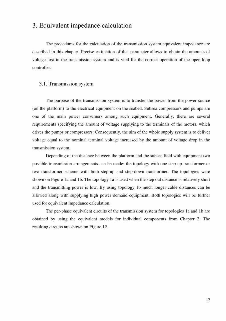
Figure 12 – Equivalent circuits of the transmission system
where
� .;[–voltage after the frequency converter,
�\]����\�– step-up transformer primary and secondary side impedance,
�\-– step-up transformer magnetizing branch impedance,
�^�– subsea cable series impedance,
�^^�����^^�– subsea cable shunt impedance,
��\]�����\�– subsea transformer primary and secondary side impedance,
��\-– subsea transformer magnetizing branch impedance,
_���_`– motor terminals.
3.2. Per-unit system
Due to the presence of step-up and subsea transformers the circuits on Figure 12 contain
several voltage levels. The calculations with the real values of parameters will be complex and
cumbersome. It is therefore convenient to express all the parameters in the per-unit system.
In per-unit system all the parameters are presented as decimal fractions or multiples of
base quantities [4]. It is widely used to choose apparent power aband line voltage �bas the main
base quantities and calculate the rest base parameters from the combinations of these two. In
some cases, especially when dealing with transformers and rotation machines there is the need to
specify the third base quantity – base frequency �b. Expressions for finding base values of
current, impedance and flux linkage are given in Equation 14.
19
b = ab√3�b �b = �b�ab
cb = √2�b√3�2d�b" Equation 14
In presence of several voltage levels, only one is used as the “main” base value �b. The
others are calculated according to the corresponding transformer ratio (Equation 15).
�b� = �b�T\��
Equation 15
where
T\��–transformer ratio between voltage level 1 and 2.
Often impedances of the electrical equipment are already expressed in the per-unit
system. In this case the base values correspond to the nominal voltage and nominal power of that
component. The per-unit parameters should be then recalculated to the new base values used for
the whole system in order to be comparable and used in further operations as shown in Equation
16.
�b;Cf = �b.gK ab;Cfab.gK h�b.gK�b;Cfi
�
Equation 16
The application of the per-unit system provides the straightforward comparison of the
parameters of different electrical components and allows to obtain easily understandable results.
In addition, it should be noticed that the per-unit impedances are almost independent of the
component voltage and power ratings. This is useful when the real parameters for some of the
equipment are unknown [17].
3.3. Thevenin equivalent
To conduct the circuit analysis and find the voltage drop in the transmission system, some
simplifications need to be made. The Thevenin theorem states that any electrical circuit
regardless of its complexity can be replaced by the simple Thevenin equivalent circuit with only
20
one impedance �\j and voltage source �\j (Figure 14e). The voltage between the nodes M and
M' remains the same both in Thevenin equivalent and the original circuit.
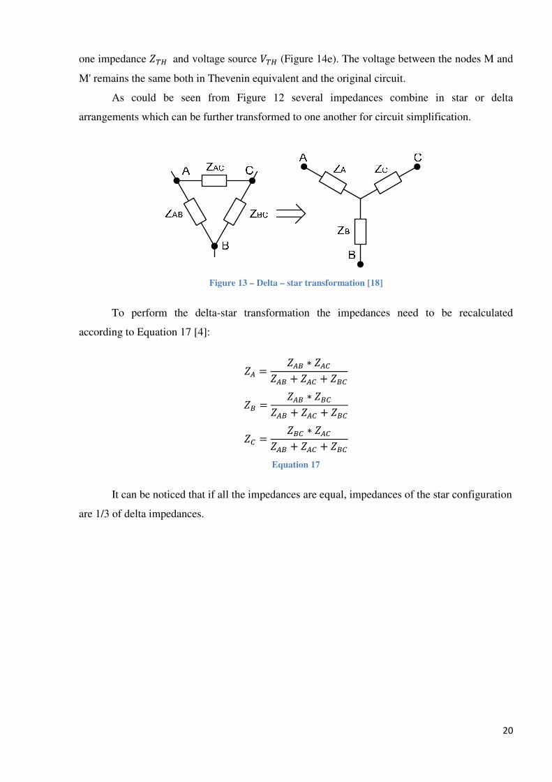
As could be seen from Figure 12 several impedances combine in star or delta
arrangements which can be further transformed to one another for circuit simplification.
Figure 13 – Delta – star transformation [18]
To perform the delta-star transformation the impedances need to be recalculated
according to Equation 17 [4]:
�k = �kb ∗ �k^�kb + �k^ + �b^
�b = �kb ∗ �b^�kb + �k^ + �b^
�^ = �b^ ∗ �k^�kb + �k^ + �b^
Equation 17
It can be noticed that if all the impedances are equal, impedances of the star configuration
are 1/3 of delta impedances.
21
Vconv
ZTP
ZTM
ZTS ZCS
ZCC1 ZCC2
A C
B
Vconv
ZTP
ZTM
ZTS ZA ZCA C
B
ZB
ZATS
Vconv
ZTP
ZTM
ZAC
ZAB ZBC
A C
B
Vconv
ZTP ZA2 ZC2A C
B
ZB2
ZA2TP
VTH
ZTH
a).
b).
c).
d).
e).
M
M'
M
M'
M
M'
M
M'
M
M'
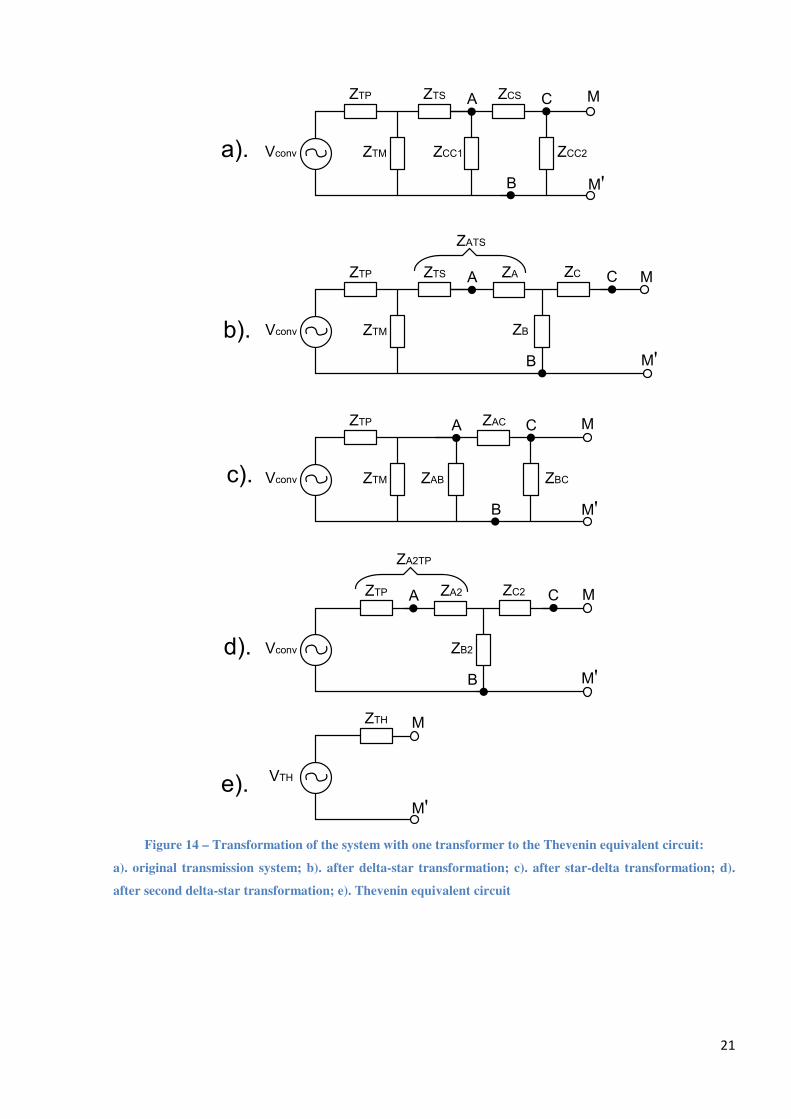
Figure 14 – Transformation of the system with one transformer to the Thevenin equivalent circuit:
a). original transmission system; b). after delta-star transformation; c). after star-delta transformation; d).
after second delta-star transformation; e). Thevenin equivalent circuit
22
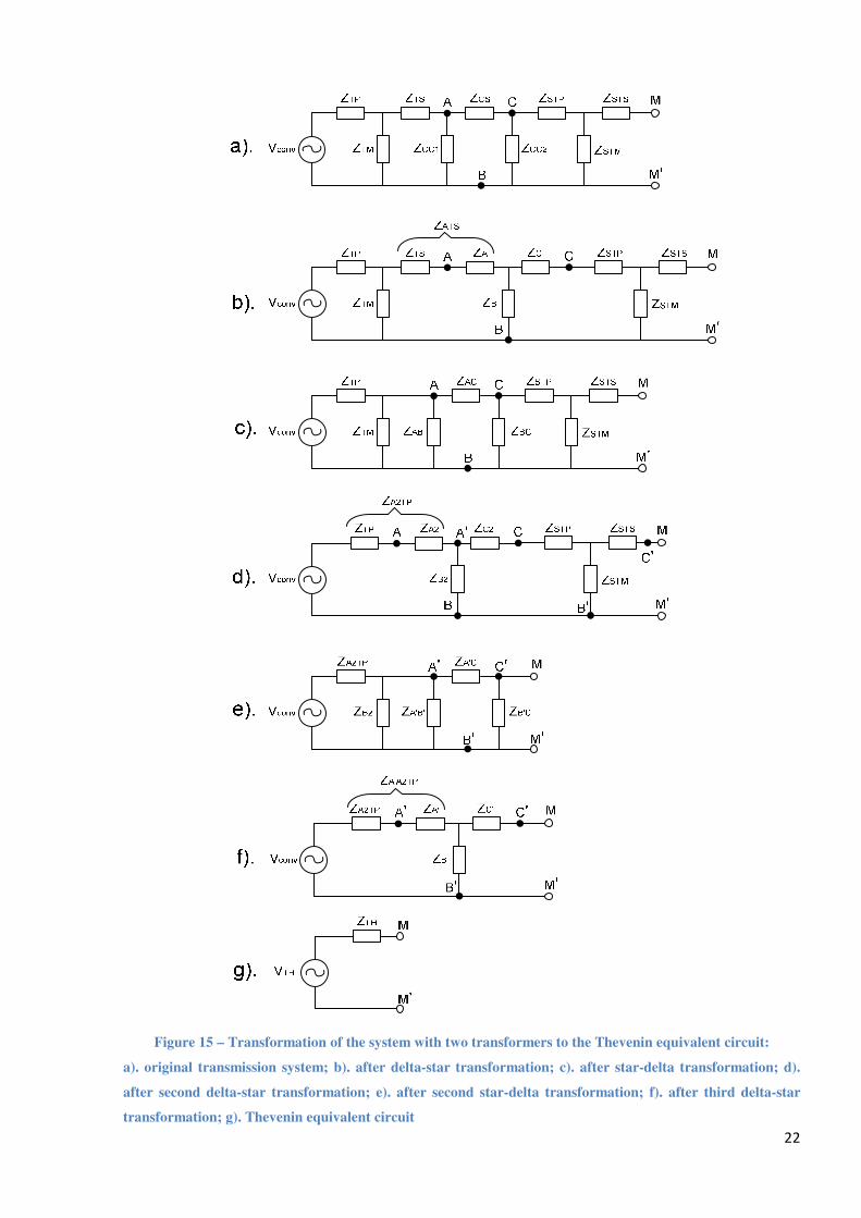
Figure 15 – Transformation of the system with two transformers to the Thevenin equivalent circuit:
a). original transmission system; b). after delta-star transformation; c). after star-delta transformation; d).
after second delta-star transformation; e). after second star-delta transformation; f). after third delta-star
transformation; g). Thevenin equivalent circuit

23
The reverse star-delta transformation is done with the help of Equation 18 [4]:
�kb = �k ∗ �b + �k ∗ �^ + �b ∗ �^�^
�b^ = �k ∗ �b + �k ∗ �^ + �b ∗ �^�k
�k^ = �k ∗ �b + �k ∗ �^ + �b ∗ �^�b
Equation 18
By using these two transformations the circuits on Figure 12 can be simplified. Figure 14
and Figure 15 indicate the necessary steps performed in order to obtain the Thevenin equivalent
circuit. As could be seen from these figures steps a). to d). are identical for both topologies.
The Matlab script was written to calculate all the parameters in the per-unit values and
find the Thevenin voltage and impedance. It can be found in Appendix A and B.
3.4. Results
The equivalent impedance obtained as a result of all the transformations can be compared
to the impedance of the simplified transmission system circuit on Figure 16. The cable charging
capacitances as well as the magnetizing branches of both transformers are omitted allowing to
simply sum up all the series impedances.
Figure 16 – Simplified circuits of the transmission system
24
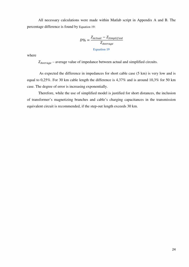
All necessary calculations were made within Matlab script in Appendix A and B. The
percentage difference is found by Equation 19:
l% = �k /n�g − ��o�YgoRoCK�k[C0�pC
Equation 19
where
�k[C0�pC – average value of impedance between actual and simplified circuits.
As expected the difference in impedances for short cable case (5 km) is very low and is
equal to 0,25%. For 30 km cable length the difference is 4,37% and is around 10,3% for 50 km
case. The degree of error is increasing exponentially.
Therefore, while the use of simplified model is justified for short distances, the inclusion
of transformer’s magnetizing branches and cable’s charging capacitances in the transmission
equivalent circuit is recommended, if the step-out length exceeds 30 km.
25
4. Start-up procedure
This chapter introduces the principles for AC motor start-up and shows the challenges
occurring during that procedure.
4.1. Motor start-up
To start the rotation the subsea motor should overcome the stiction torque. Its magnitude
can vary significantly depending of the system. In this master thesis the worst scenario is
analyzed: stiction torque equals to 0,3 pu of the nominal value. As was already mentioned in the
system description the motor is supplied through FC, which makes possible to use control
technique similar to V/f control. The main idea is to supply the motor with the voltage at low
frequency at the beginning and then gradually increasing both V and f. The low initial frequency
allows the substantial reduction of the starting currents, which can be 4-7 times higher than the
rated value [1].
The V/f ratio should be constant in order to keep the transformer under the saturation. If
motor is supplied through the long cable with high impedance, the terminal voltage of the
machine is not enough for overcoming the stiction. In this case, the additional voltage called
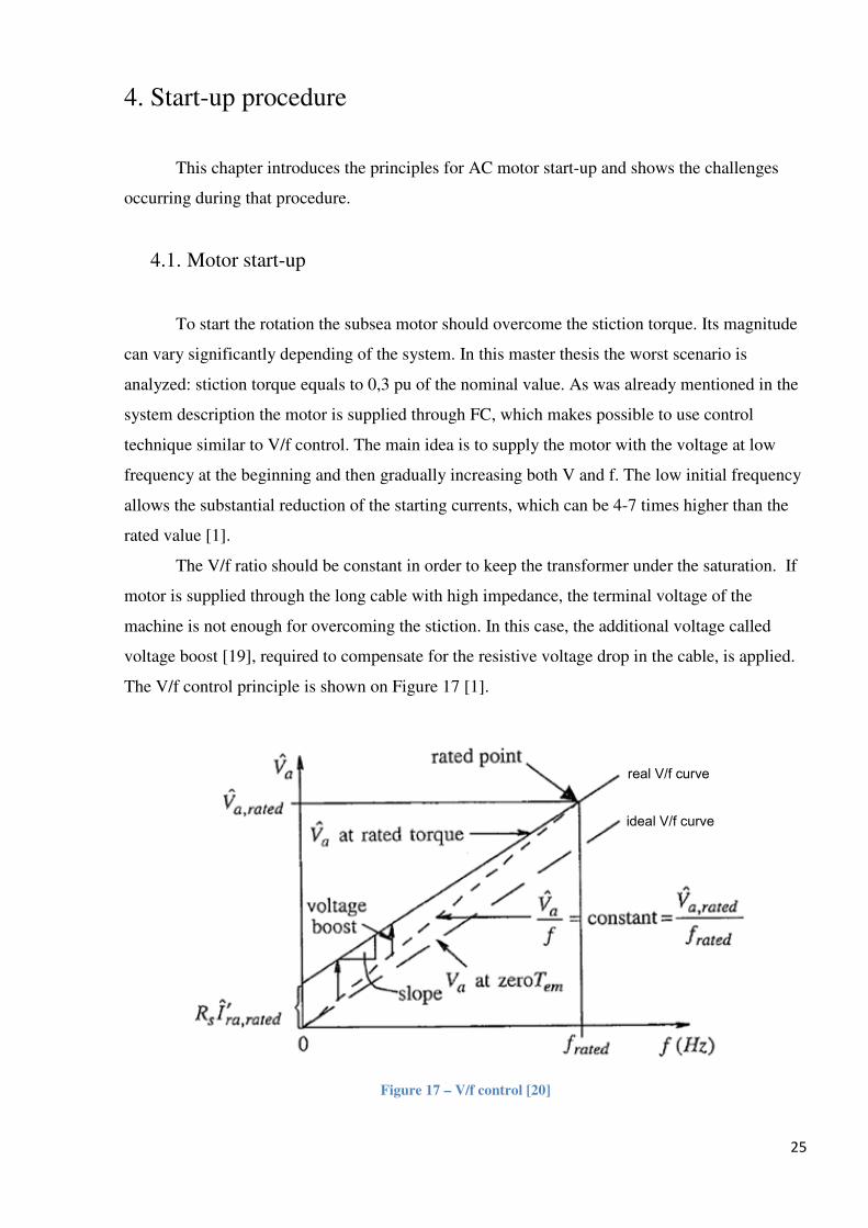
voltage boost [19], required to compensate for the resistive voltage drop in the cable, is applied.
The V/f control principle is shown on Figure 17 [1].
real V/f curve
ideal V/f curve
Figure 17 – V/f control [20]
26
From Figure 17 it is seen that the resistive part of the transmission system and machine
itself offsets the V/f curve from the ideal one, so that motor will not be able to achieve nominal
voltage at nominal frequency. With the voltage boosting the ideal characteristic is shifted
towards the real curve and thus enough voltage is supplied to the motor.
With the voltage boost the V/f ratio become larger than the rated value and cause the
proportional increase in the transformer flux. If this new flux is exceeding the maximum flux
value for the transformer, the size of the transformer core should be increased to avoid the
saturation [2].
The working principle of the controller used for this project is similar to V/f control with
the aim of compensating the voltage drop in the transmission system at any frequency, thus
always supplying enough voltage on machine’s terminal. The frequency is ramping up from
initial to rated value. To decouple the motor’s torque and flux, the d-q reference frame is used.
For PM machine voltage supplied to the terminals is calculated using following equations:
�K = �J/0� + JK" �OK�' + ��/0� + �"OK − JK= OL
�L = NJ/0� + JLP �OL�' + ��/0� + �"OL + JK= OK +c= JL
Equation 20
where
JK ���JL– inductance in d and q axis, with non-salient pole machine JK =JL,
�/0����J/0�– resistance and inductance of the transmission system, calculated in
Chapter 3,
c– magnetic flux induced by the permanent magnets.
Although this set of equations is written for PM machine, it can be used to control IM as
well. The Simulink model of controller based on these formulas is shown in Chapter 5.
4.2. Transformer saturation
The transformer core is made of the ferromagnetic material, usually iron. Such materials
consist of the areas called magnetic domains. Each of these domains has a strong magnetic field,
but due to their different orientation in space, the total magnetization is zero.
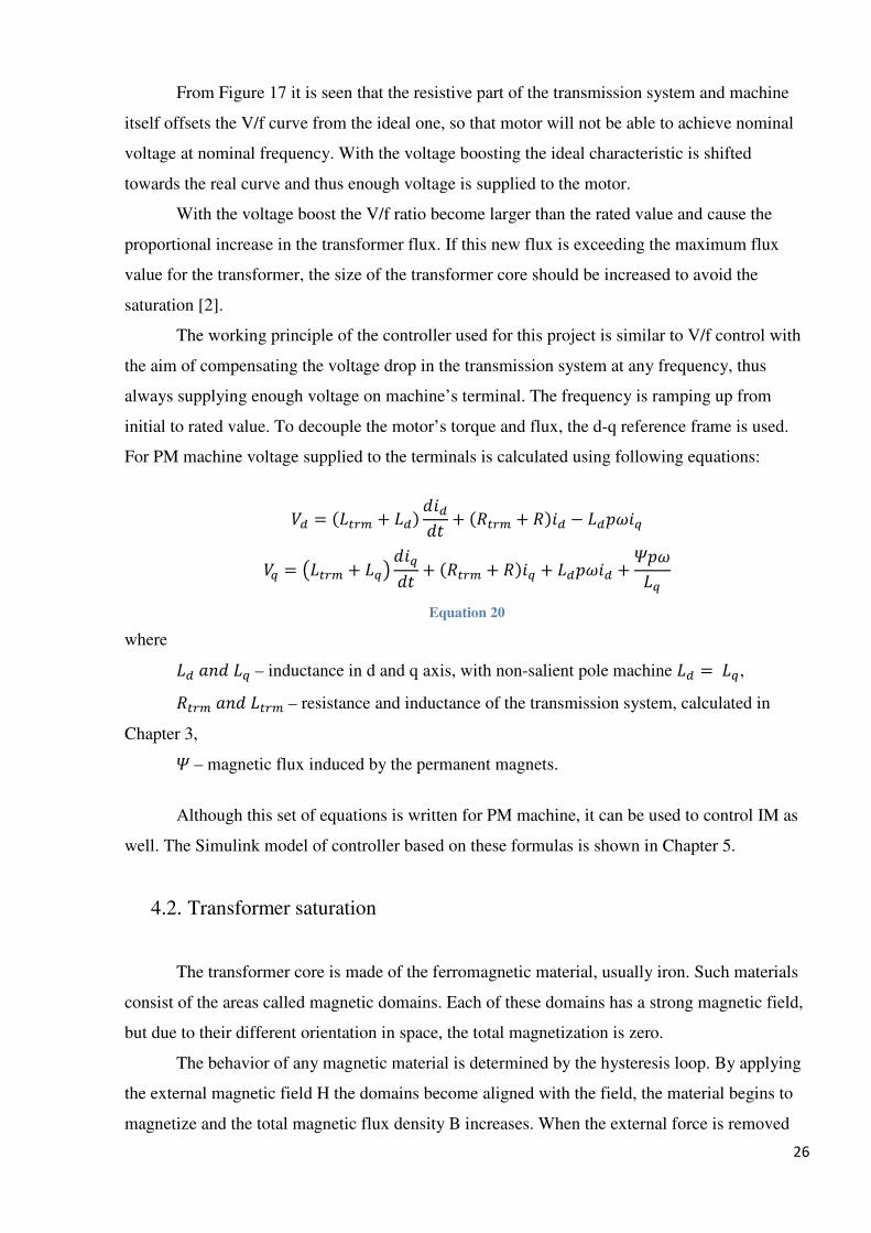
The behavior of any magnetic material is determined by the hysteresis loop. By applying
the external magnetic field H the domains become aligned with the field, the material begins to
magnetize and the total magnetic flux density B increases. When the external force is removed
27
from the ferromagnetic material, it will still have some remaining magnetization – retentivity.
This effect is called hysteresis. To remove the magnetization completely the oppose magnetic
field with the coercivity force should be applied [1].
Within certain range the B and H in the core have linear relationship. However, at some
point the further increasing of the magnetic field H will not cause the proportional increasing of
the magnetization, because all of the domains are already properly aligned. This state is called
saturation and has undesirable effects on the transformer operation.
The typical B-H hysteresis loop is shown on Figure 18.
Figure 18 – B-H hysteresis loop [21]
The value of the operating flux density of the core will influence the overall size, material
cost and transformer performance [22]. After approximately 1,9 T of the flux density B, the
characteristics become worse, so with the 10% margin the operating limit for the flux density can
be set to 1,73 T.
The transformer saturation can be easily observed by inspecting the magnetizing currents
graphs.
28
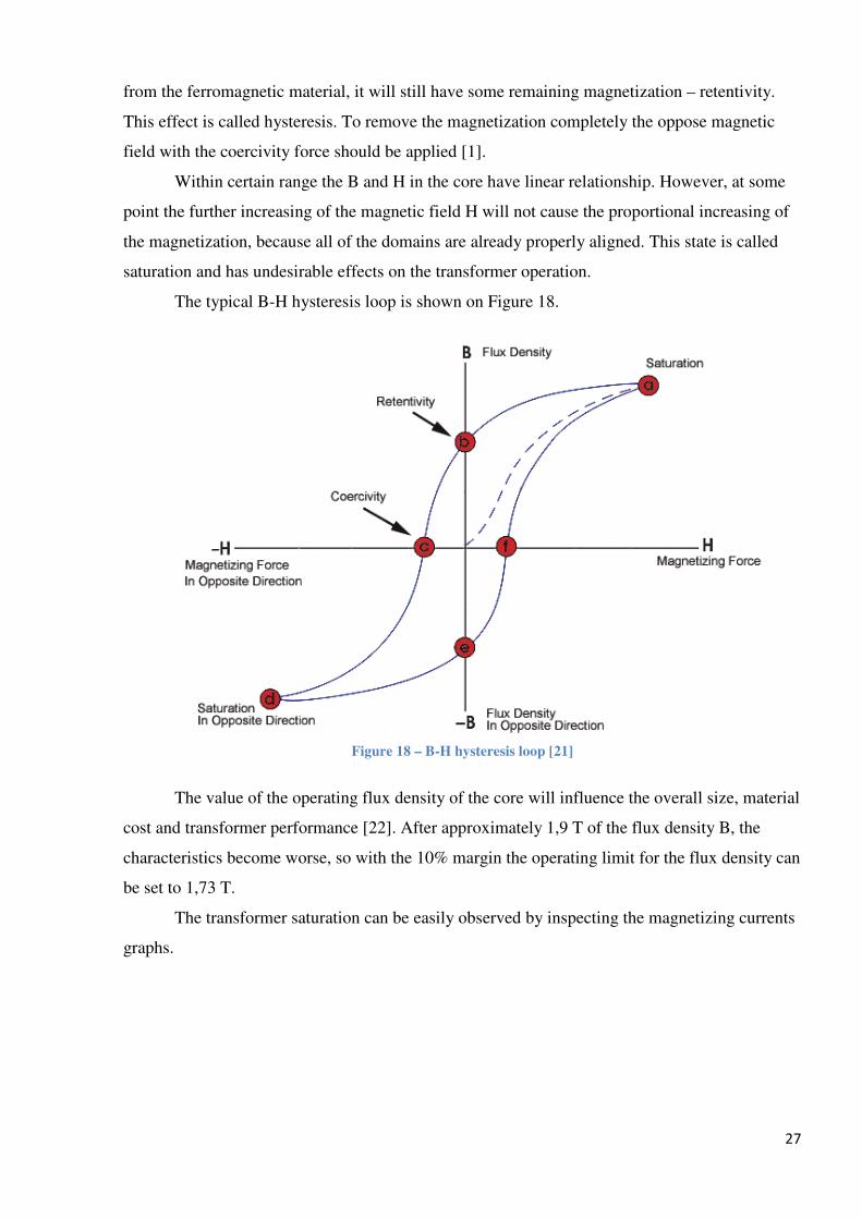
Figure 19 – Effect of transformer saturation
On the figure: top graph: y-axis – transformer flux, [pu]; bottom graph: y-axis – magnetizing current, [pu] ; x-axis –
time, [s].
As could be seen from Figure 19 when the flux in the transformer is under or equal to 1
pu, the magnetizing current almost insignificant. When the flux in phases A (black color) and B
(pink color) exceeds the rated value, transformer enters the saturation, which results in rapid
increase of the magnetizing current (of the corresponded phases) to the magnitudes comparable
with the load current flowing in the system.
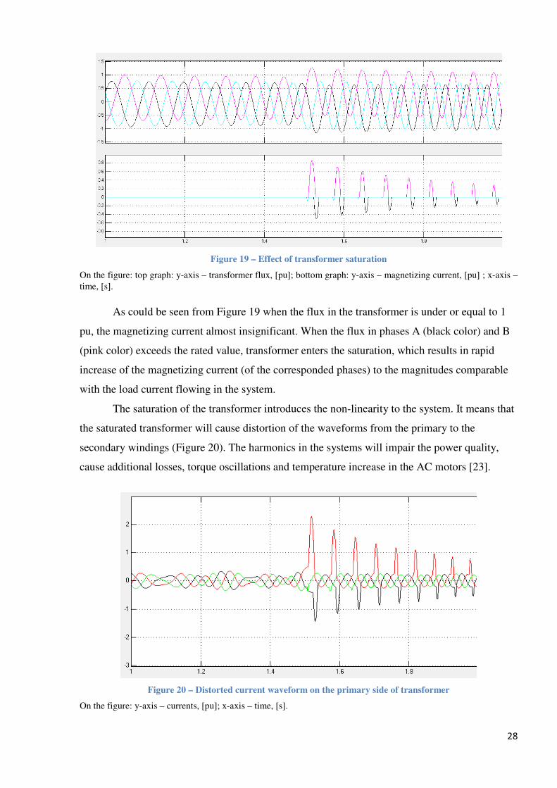
The saturation of the transformer introduces the non-linearity to the system. It means that
the saturated transformer will cause distortion of the waveforms from the primary to the
secondary windings (Figure 20). The harmonics in the systems will impair the power quality,
cause additional losses, torque oscillations and temperature increase in the AC motors [23].
Figure 20 – Distorted current waveform on the primary side of transformer
On the figure: y-axis – currents, [pu]; x-axis – time, [s].
29
4.3. Start-up limitations
As was already mentioned, IM can be started with some initial frequency. There are two
factors that used to determine that starting frequency [24]: the maximum flux in the transformer
and the maximum current coming through the Frequency Converter (FC).
By using equations given in section for induction motor and rearranging them (Equation
21) it is possible to obtain curves that show the relations between current-frequency (speed) and
flux – frequency [25].
c�/�0/o;p ≅ S 23= B9/�0/o;pN�CL� + �CL� P�0 ∗ 2d�9
09/�0o;p = S=2B9/�0/o;p2d�93�0
Equation 21
where
�CL– equivalent resistance equal to �CL = �\j/0�;9 + �/>r-,
�\j/0�;9 – resistive part of Thevenin impedance for transmission system,
�/>r- – resistive part of Thevenin impedance for IM circuit (Figure 8),
�CL– equivalent reactance equal to �CL = �\j/0�;9 + �/>r-,
�\j/0�;9 – reactive part of Thevenin impedance for transmission system,
�/>r- – reactive part of Thevenin impedance for IM circuit (Figure 8),
�9– stator frequency,
B9/�0/o;p– starting torque, equal to stiction torque.
For the given machine power and nominal speed the value of the stiction torque in Nm
can be calculated through Equation 22 [25]:
B9/o /o.; = 0.3 ∗ BC�,0�/CK = 0.3 ∗ 1-./.0 9
Equation 22
From Equation 22 the stiction torque B9/o /o.; = 2388�t with the rated torque be equal
to BC�,0�/CK = 7957,75�t.
30
As could be seen there is no slip in the formulas of Equation 21. This is because the
formulas are written for starting conditions, when the slip always equals to 1. By putting �9 changing from 0 to the rated value (100 Hz in this study) and using the value of the stiction
torque for B9/�0/o;p , one can see what levels of currents and fluxes can be expected in the system
at any starting frequency.
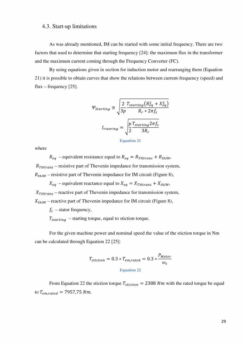
Curves for starting of the system with 5km cable and IM shown on Figure 21. The
corresponding Matlab script can be found in Appendix C.
Figure 21 – Flux and current curves for 5km cable
On the figure: y-axis – flux/current, [pu]; x-axis – frequency, [Hz].
The obtained flux represents the flux in the transformer due to the use of the aggregate
impedance of transmission system together with motor itself in the Equation 21. The values of
the motor flux will be lower. The current on the curve is the current flowing in the machine’s
rotor, but it can be considered equal to the one going through FC.
As expected the starting currents are decreasing, if the motor is starting with lower
frequency. The fluxes, however, are very high at low frequency, since the flux is the integral of
voltage over time. The selection of the initial frequency according to Figure 21 is a tradeoff
between these two quantities. The curves also show that some oversizing of either transformer
core or converter is required in order to start-up this system.
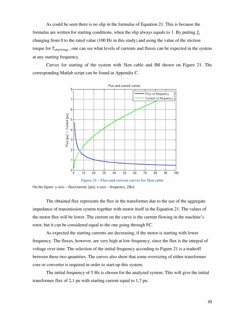
The initial frequency of 5 Hz is chosen for the analyzed system. This will give the initial
transformer flux of 2,1 pu with starting current equal to 1,7 pu.
31
Figure 22 – Flux and current curves for 5km cable
On the figure: y-axis – flux/current, [pu]; x-axis – frequency, [Hz].
4.4. Inrush currents and transformer bypass
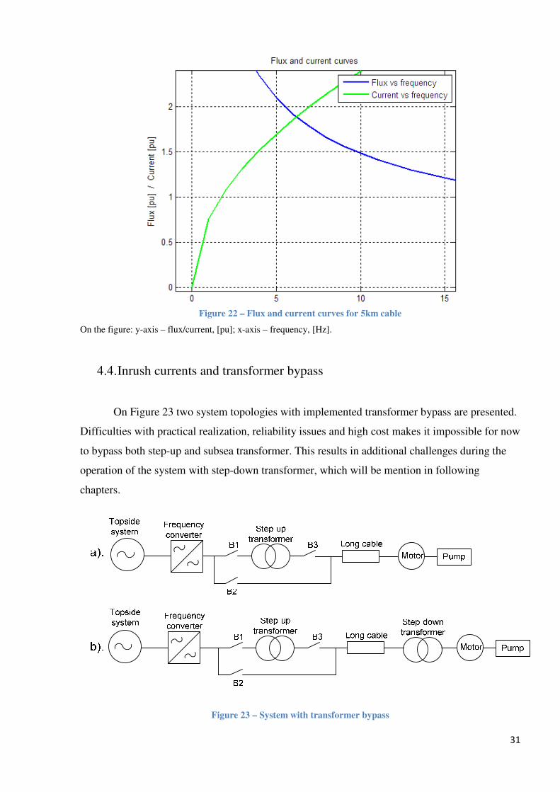
On Figure 23 two system topologies with implemented transformer bypass are presented.
Difficulties with practical realization, reliability issues and high cost makes it impossible for now
to bypass both step-up and subsea transformer. This results in additional challenges during the
operation of the system with step-down transformer, which will be mention in following
chapters.
Figure 23 – System with transformer bypass
32
To ensure the stable operation of the system with bypass, close attention should be paid
to evaluate the closing/opening times of the breakers.
The scheme utilizes three circuit breakers, which gives the possibility of providing an
alternative path for the power going from the FC to the motor. Though it seems that two breakers
are enough for creating the bypass, it was investigated that without breaker B3 the transformer
can be saturated from the motor side. Thus three breakers are installed.
In the beginning of the start-up with transformer bypass, breaker B1 is closed, while the
bypass breaker B2 and breaker B3 are open. This allows transformer pre-magnetization, which
will be explained further. After magnetization, B1 opens and B2 goes to the closed position.
Now the power flows directly from the FC to the motor, avoiding the transformer. After the
machine reaches certain speed, B2 opens and breakers B1 and then B3 become close. As will be
proven by the simulation, some delay between breakers operation is acceptable and they do not
need to be precisely synchronized with each other. The only requirement for the B3 is to avoid
the saturation of the transformer from the motor side, when it is closing [1].
The sudden reconnection of the transformer can cause the high currents flowing in it.
This occurs, if the residual flux in the core does not match the instantaneous flux value for the
point of voltage waveform, when the reconnection is done [26], [1]. In the analyzed system it
was estimated, that the inrush currents do not always represent an issue, because the switching
occurs when the voltage magnitude is much lower than rated value and therefore the inrush
current magnitude will be moderate as well.
Another consequence of sudden reconnection of transformer is an appearance of DC
offset in the flux. It will appear according to Equation 23 [27]:
c�'" = c�7O�� ' + 8" + c�0" − c�7O��8" Equation 23
where
c�– amplitude of the flux,
c�0"– residual flux,
8– phase angle.
The amplitude of the flux at reconnection can be equal to 2c� +c�0" in the worst case.
The magnitude of DC component is depending on the initial flux c�0"and phase angle at which
the switching occurs. High DC component can drive transformer into the saturation, so it is very
important to reconnect the transformer at right phase angle. Consider the following figures
33
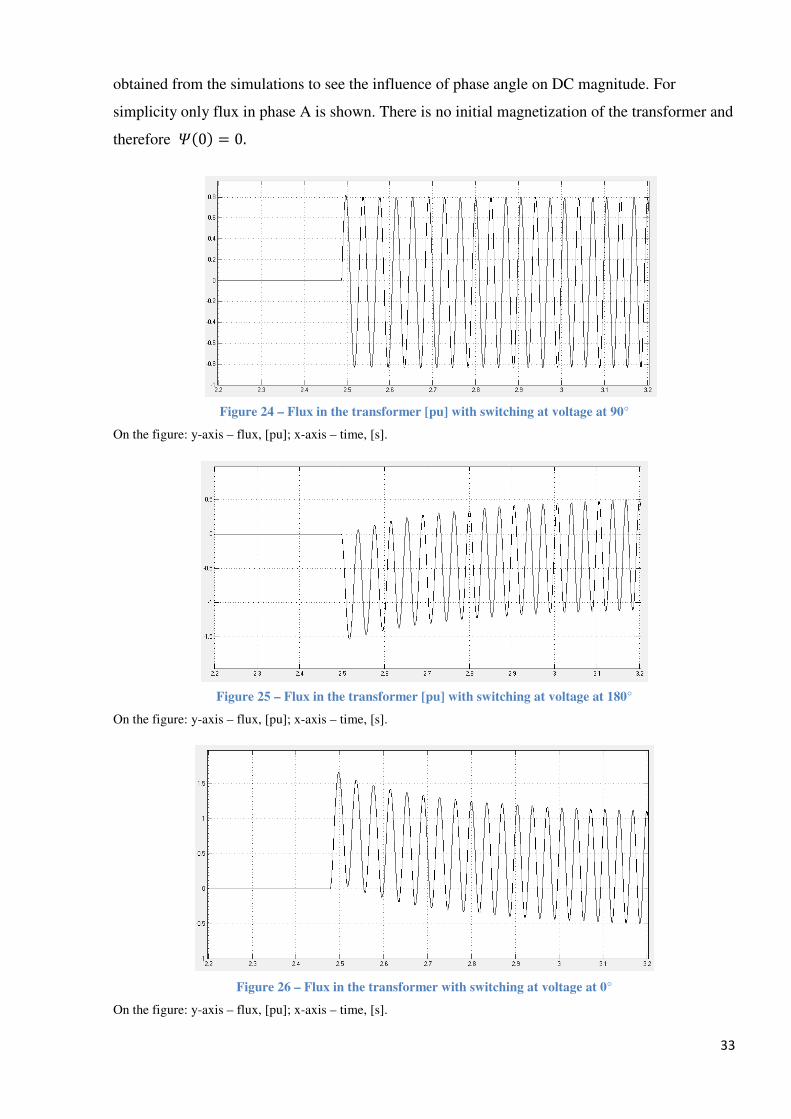
obtained from the simulations to see the influence of phase angle on DC magnitude. For
simplicity only flux in phase A is shown. There is no initial magnetization of the transformer and
therefore c�0" = 0.
Figure 24 – Flux in the transformer [pu] with switching at voltage at 90°
On the figure: y-axis – flux, [pu]; x-axis – time, [s].
Figure 25 – Flux in the transformer [pu] with switching at voltage at 180°
On the figure: y-axis – flux, [pu]; x-axis – time, [s].
Figure 26 – Flux in the transformer with switching at voltage at 0°
On the figure: y-axis – flux, [pu]; x-axis – time, [s].

34
From Figure 24-26 it can be seen, that switching at voltage phase angle equal to 0° or
180° will cause the DC offset. The best result is obtained when switching is occurred at 90°
phase angle. There is almost no DC component in the transformer flux.
In the system all three phases will be switched on instantaneously. If the phase A is
switched on at 90°, the phase angles for the rest two phases will be shifted by 120° due to the
symmetry. The way of eliminating the DC component in the fluxes is pre-magnetization of
transformer. By magnetizing the transformer core in a certain way before actual system start-up,
the residual fluxes c�0" will cancel out the induced DC component due to phase angles right
after the reconnection. As was already mentioned the pre-magnetization is done, when only
breaker B1 is in closed position.
35
5. Simulink models
The systems, build for the motor start-up simulations, are mainly compose of the premade
models found in the Matlab/Simulink library. However, in case of the power source and motor
load blocks the new models were made in order to meet the requirements of the current work.
These models are further discussed in this chapter.
5.1. Power source model
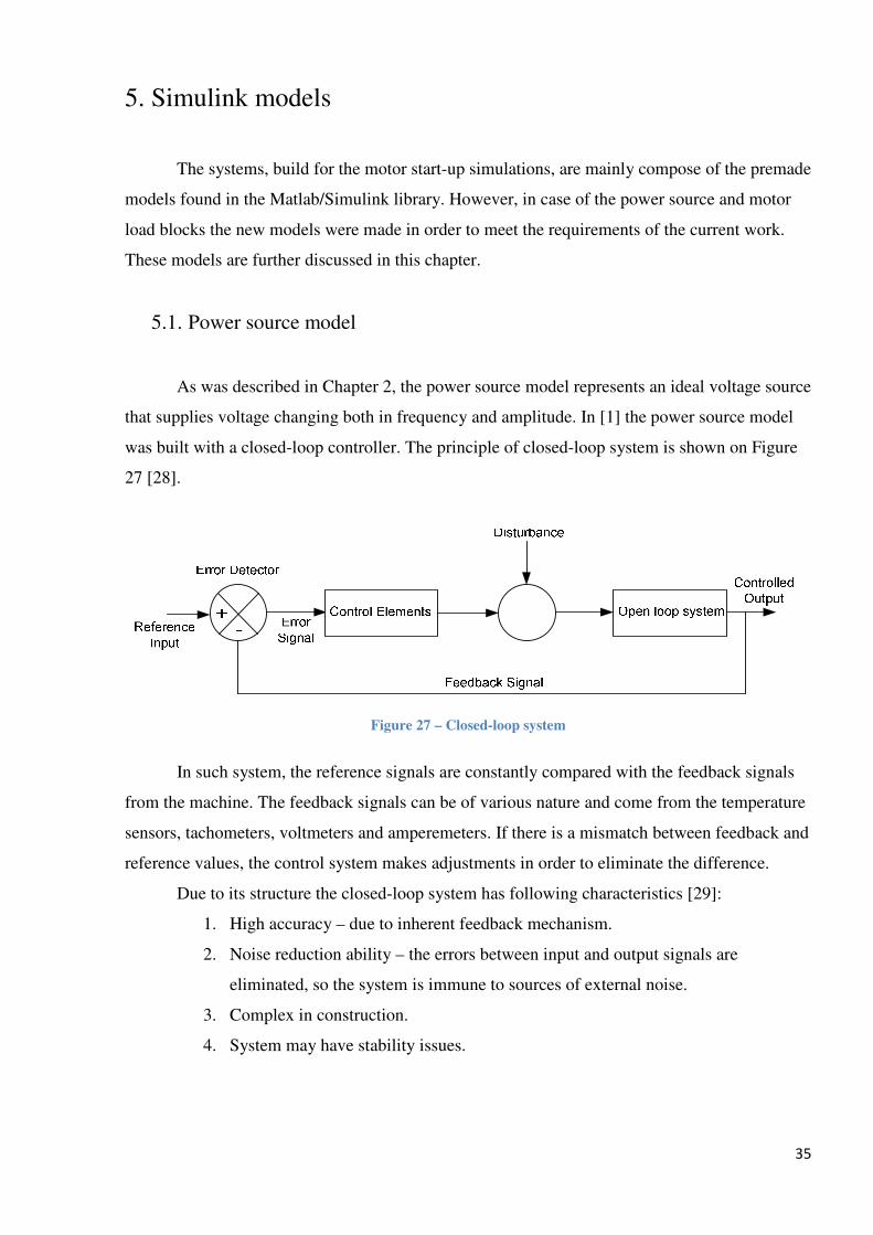
As was described in Chapter 2, the power source model represents an ideal voltage source
that supplies voltage changing both in frequency and amplitude. In [1] the power source model
was built with a closed-loop controller. The principle of closed-loop system is shown on Figure
27 [28].
Figure 27 – Closed-loop system
In such system, the reference signals are constantly compared with the feedback signals
from the machine. The feedback signals can be of various nature and come from the temperature
sensors, tachometers, voltmeters and amperemeters. If there is a mismatch between feedback and
reference values, the control system makes adjustments in order to eliminate the difference.
Due to its structure the closed-loop system has following characteristics [29]:
1. High accuracy – due to inherent feedback mechanism.
2. Noise reduction ability – the errors between input and output signals are
eliminated, so the system is immune to sources of external noise.
3. Complex in construction.
4. System may have stability issues.

36
Although the closed-loop system allows precise control of the motor, the relatively high
cost, necessity of installing sensors and decreased reliability makes such systems less favorable
choice when it comes to use in the subsea industry. To operate the motor placed on the seabed,
the open-loop system is used instead (Figure 28). Such system is cheaper to construct and its
simplicity grants improved stability.
Figure 28 – Open-loop system
In the open-loop system there is no feedback signals from the object. Evaluation of the
system response is possible only in indirect way. Since the system cannot adjust itself, the
selection of the initial settings should be done very carefully. In case of the open-loop controller
used in this master thesis, there is a need of precise and accurate estimation of equivalent
impedances of system components in order to provide adequate amount of voltage to the motor’s
terminals. This will represent a challenge for the real systems, where impedances depend on the
components state and environment in which installation is placed.
Since the open-loop controller is a more realistic option for subsea motor starting, it was
chosen for the use in this work.
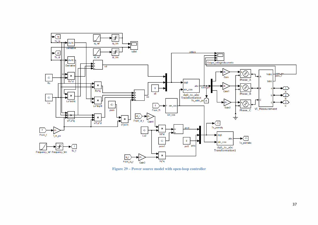
The open-loop controller model is based on formulas in Equation 20 and its Simulink
representation is shown on Figure 29. The block “Frequency_ref” gives linearly increasing
frequency from initial value to the rated value. By using blocks “iq_ref” and “id_ref” the voltage
in dq – axis is influenced. Using dq reference frame allows to decouple the motor’s torque and
flux from each other. Iq is controlling the torque, Id – flux. Block “psim” introduce the flux
linkage from the permanent magnets.
To supply the three phase voltages to the system, voltages Vd and Vq calculated using
the equivalent impedances from Chapter 3 and reference currents “iq_ref” and “id_ref”. Then
these two voltages transform from dq to abc reference frame with the Park transformation
(Equation 25 for direct and Equation 25 for reverse trasformation).
37
Figure 29 – Power source model with open-loop controller
38
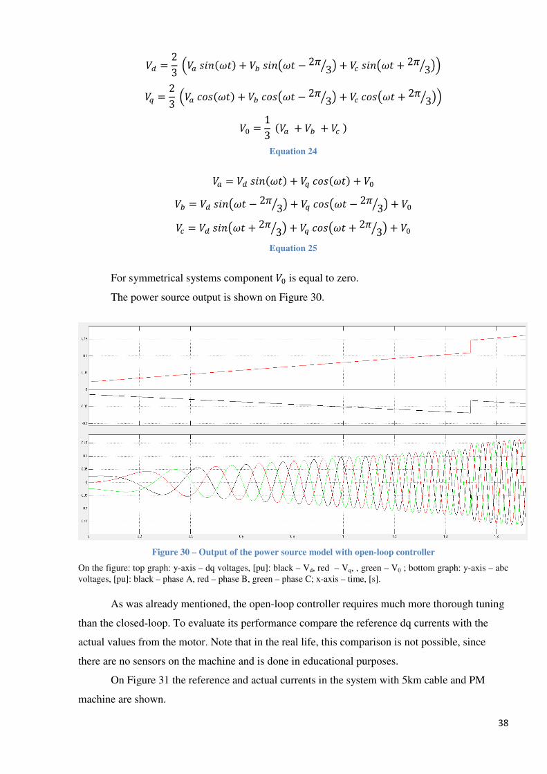
�K = 23@��7O�� '" + �x7O�N ' − 2d 3y P + � 7O�N ' + 2d 3y PA �L = 23@��567� '" + �x567N ' − 2d 3y P + � 567N ' + 2d 3y PA
� = 13��� + �x + � " Equation 24
�� = �K7O�� '" + �L567� '" + � �x = �K7O�N ' − 2d 3y P + �L567N ' − 2d 3y P + � � = �K7O�N ' + 2d 3y P + �L567N ' + 2d 3y P + �
Equation 25
For symmetrical systems component � is equal to zero.
The power source output is shown on Figure 30.
Figure 30 – Output of the power source model with open-loop controller
On the figure: top graph: y-axis – dq voltages, [pu]: black – Vd, red – Vq, , green – V0 ; bottom graph: y-axis – abc
voltages, [pu]: black – phase A, red – phase B, green – phase C; x-axis – time, [s].
As was already mentioned, the open-loop controller requires much more thorough tuning
than the closed-loop. To evaluate its performance compare the reference dq currents with the
actual values from the motor. Note that in the real life, this comparison is not possible, since
there are no sensors on the machine and is done in educational purposes.
On Figure 31 the reference and actual currents in the system with 5km cable and PM
machine are shown.
39
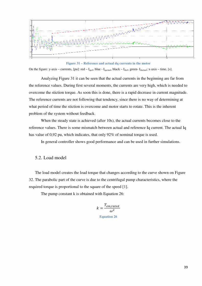
Figure 31 – Reference and actual dq currents in the motor
On the figure: y-axis – currents, [pu]: red – Iqref, blue - Iqactual, black – Idref, green- Idactual; x-axis – time, [s].
Analyzing Figure 31 it can be seen that the actual currents in the beginning are far from
the reference values. During first several moments, the currents are very high, which is needed to
overcome the stiction torque. As soon this is done, there is a rapid decrease in current magnitude.
The reference currents are not following that tendency, since there is no way of determining at
what period of time the stiction is overcome and motor starts to rotate. This is the inherent
problem of the system without feedback.
When the steady state is achieved (after 10s), the actual currents becomes close to the
reference values. There is some mismatch between actual and reference Iq current. The actual Iq
has value of 0,92 pu, which indicates, that only 92% of nominal torque is used.
In general controller shows good performance and can be used in further simulations.
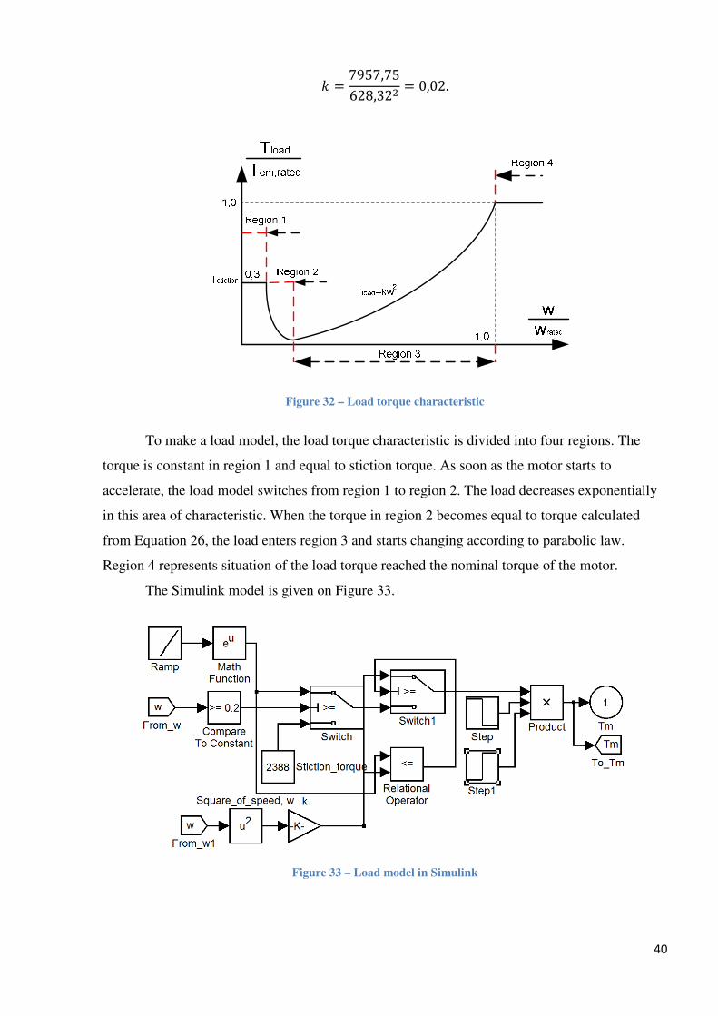
5.2. Load model
The load model creates the load torque that changes according to the curve shown on Figure
32. The parabolic part of the curve is due to the centrifugal pump characteristics, where the
required torque is proportional to the square of the speed [1].
The pump constant k is obtained with Equation 26:
T = BC�,0�/CK �
Equation 26
40
T = 7957,75628,32� = 0,02.
Figure 32 – Load torque characteristic
To make a load model, the load torque characteristic is divided into four regions. The
torque is constant in region 1 and equal to stiction torque. As soon as the motor starts to
accelerate, the load model switches from region 1 to region 2. The load decreases exponentially
in this area of characteristic. When the torque in region 2 becomes equal to torque calculated
from Equation 26, the load enters region 3 and starts changing according to parabolic law.
Region 4 represents situation of the load torque reached the nominal torque of the motor.
The Simulink model is given on Figure 33.
Figure 33 – Load model in Simulink

41
Simulink blocks “Step” and “Step1” can be used to simulate sudden increase or decrease
of the load.
The torque created by the load model is given on Figure 34.
Figure 34 – Load torque
On the figure: y-axis – load torque, [Nm]; x-axis – time, [s].
In practice the torque reduction in region 2 is so rapid, it is seen almost as instantaneous.
At 12s the load is decreased with the use of blocks “Step” and “Step1”. In next chapter this will
be used to analyze the system behavior in case of sudden load change.
42
6. Simulation results
This chapter displays the results obtained from the simulation models of the system
shown on Figure 1a and b. Both IM and PM machine are tested and their behavior analyzed.
Four cases are considered:
1. Case 1 – system with step-up transformer and 5km cable;
2. Case 2 – system with both step-up and step-down (subsea) transformers. Cable
lengths of 30 and 50km are simulated;
3. Case 3 – implementing transformer bypass suggested by SmartMotor AS into the
system from Case 1 (Figure 23a).
4. Case 4 – testing of transformer bypass on the system from Case 2 (Figure 23b).
Transformer bypass solution is tested in Cases 3 and 4 in order to conclude about its
feasibility and possibility for practical realization. The results from each case are discussed and
comments on them are given.
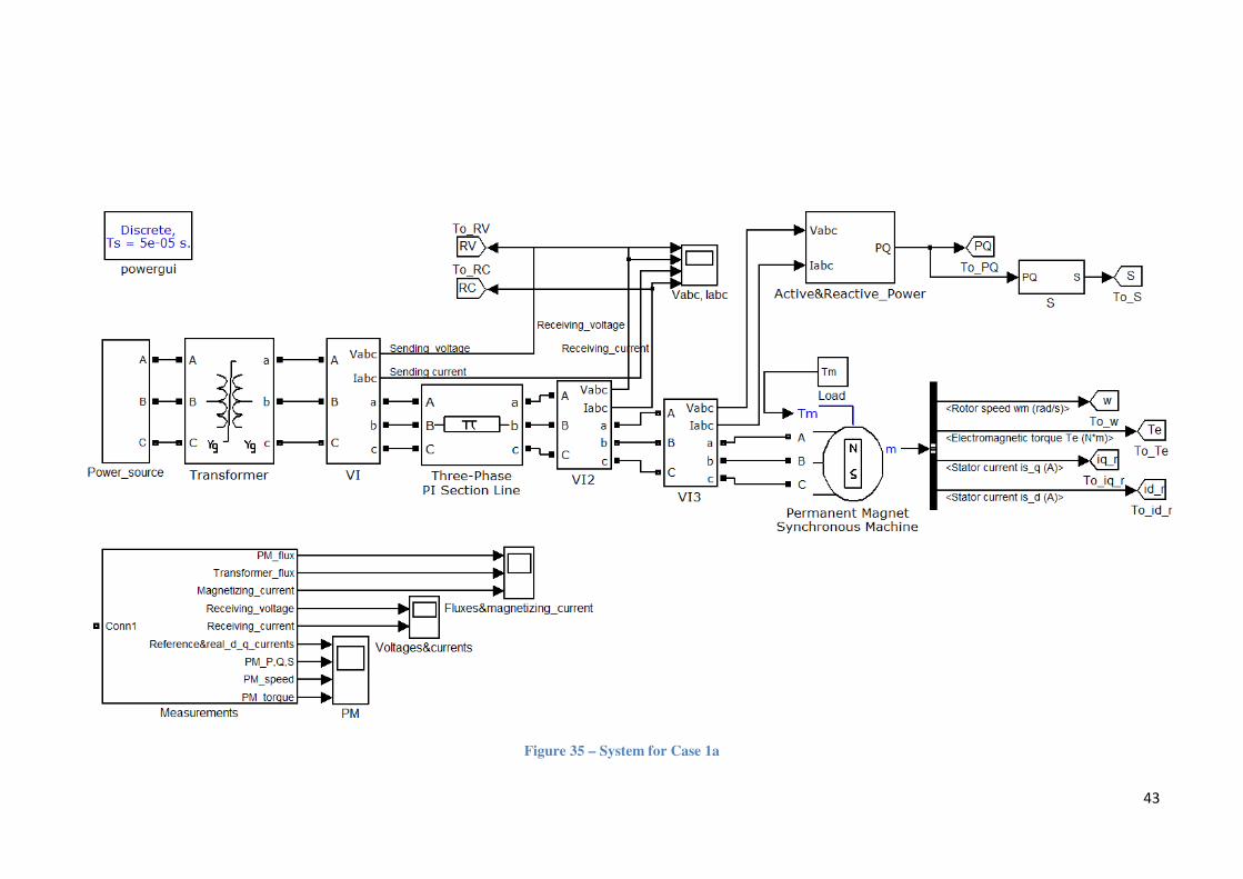
6.1. Case 1a – Start-up of PM with step-up transformer
The system for Case 1a is given on Figure 35. Due to the voltage drop requirements
(∆�should not exceed 15-20% for such system) cable length of no more than 5km is allowed.
Large voltage drop caused by 5 MW PM motor, which is relatively high power to be transmitted
through the cable on voltage level of 6,6 kV.
On Figure 36 the motor parameters are presented. The actual and reference dq currents
and their behavior were discussed in previous chapter. It can be seen that there is a good match
between real and actual values at steady state. From the speed graph it can be observed that the
motor is successfully started and at 10s reaches the rated speed equal to 2d ∗ 100 =628,32 |�� 7y . At that speed the motor active power is 5 MW and it operates with power factor
of 0,82.
The motor’s torque has large oscillations and reaches the point of equilibrium with the
load at t = 12,5s. According to [30], the reason for these oscillations is deviations from a
sinusoidal flux density distribution around the air-gap. The pre-magnetization of transformer
helps in reducing the magnitude of such oscillations, which is shown on Figure 37. Another way
of eliminating this problem is the usage of damper winding at the PM, which is beyond the scope
43
Figure 35 – System for Case 1a
44
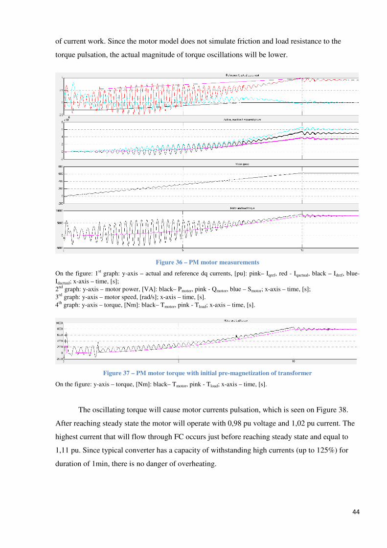
of current work. Since the motor model does not simulate friction and load resistance to the
torque pulsation, the actual magnitude of torque oscillations will be lower.
Figure 36 – PM motor measurements
On the figure: 1st graph: y-axis – actual and reference dq currents, [pu]: pink– Iqref, red - Iqactual, black – Idref, blue-
Idactual; x-axis – time, [s];
2nd
graph: y-axis – motor power, [VA]: black– Pmotor, pink - Qmotor, blue – Smotor; x-axis – time, [s];
3rd
graph: y-axis – motor speed, [rad/s]; x-axis – time, [s].
4th
graph: y-axis – torque, [Nm]: black– Tmotor, pink - Tload; x-axis – time, [s].
Figure 37 – PM motor torque with initial pre-magnetization of transformer
On the figure: y-axis – torque, [Nm]: black– Tmotor, pink - Tload; x-axis – time, [s].
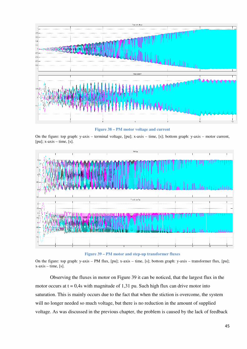
The oscillating torque will cause motor currents pulsation, which is seen on Figure 38.
After reaching steady state the motor will operate with 0,98 pu voltage and 1,02 pu current. The
highest current that will flow through FC occurs just before reaching steady state and equal to
1,11 pu. Since typical converter has a capacity of withstanding high currents (up to 125%) for
duration of 1min, there is no danger of overheating.
45
Figure 38 – PM motor voltage and current
On the figure: top graph: y-axis – terminal voltage, [pu]; x-axis – time, [s]; bottom graph: y-axis – motor current,
[pu]; x-axis – time, [s].
Figure 39 – PM motor and step-up transformer fluxes
On the figure: top graph: y-axis – PM flux, [pu]; x-axis – time, [s]; bottom graph: y-axis – transformer flux, [pu];
x-axis – time, [s].
Observing the fluxes in motor on Figure 39 it can be noticed, that the largest flux in the
motor occurs at t = 0,4s with magnitude of 1,31 pu. Such high flux can drive motor into
saturation. This is mainly occurs due to the fact that when the stiction is overcome, the system
will no longer needed so much voltage, but there is no reduction in the amount of supplied
voltage. As was discussed in the previous chapter, the problem is caused by the lack of feedback
46
in the open-loop controller. It is possible that high flux in the motor can be avoided by
optimizing the controller in the power source model.
The maximum transformer flux occurs in phase B with magnitude of 2,1 pu. DC offset in
the phase B and C is clearly observed in accordance with Equation 23. DC component is dying
out due to the losses in the transformer and is absent, when the system reaches steady state. To
avoid transformer saturation in the analyzed system, transformer core should be oversized by
factor of 2,1.
6.2. Case 1b – Start-up of IM with step-up transformer
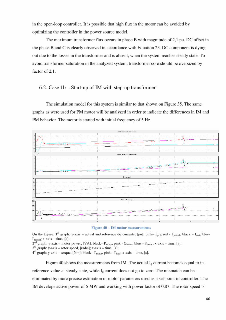
The simulation model for this system is similar to that shown on Figure 35. The same
graphs as were used for PM motor will be analyzed in order to indicate the differences in IM and
PM behavior. The motor is started with initial frequency of 5 Hz.
Figure 40 – IM motor measurements
On the figure: 1st graph: y-axis – actual and reference dq currents, [pu]: pink– Iqref, red - Iqactual, black – Idref, blue-
Idactual; x-axis – time, [s];
2nd
graph: y-axis – motor power, [VA]: black– Pmotor, pink - Qmotor, blue – Smotor; x-axis – time, [s];
3rd
graph: y-axis – rotor speed, [rad/s]; x-axis – time, [s].
4th
graph: y-axis – torque, [Nm]: black– Tmotor, pink - Tload; x-axis – time, [s].
Figure 40 shows the measurements from IM. The actual Iq current becomes equal to its
reference value at steady state, while Id current does not go to zero. The mismatch can be
eliminated by more precise estimation of motor parameters used as a set-point in controller. The
IM develops active power of 5 MW and working with power factor of 0,87. The rotor speed is
47
622,2 rad/s, which is slightly lower than the synchronous and gives the slip equal to 0,97%. This
value is typical for the IM motor of that size. Compare with PM machine, there is almost no
torque oscillation. The largest oscillation occurs right before motor reaches steady state.
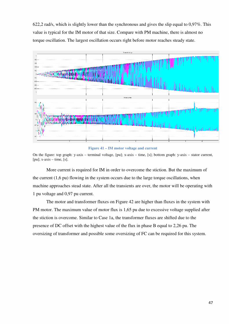
Figure 41 – IM motor voltage and current
On the figure: top graph: y-axis – terminal voltage, [pu]; x-axis – time, [s]; bottom graph: y-axis – stator current,
[pu]; x-axis – time, [s].
More current is required for IM in order to overcome the stiction. But the maximum of
the current (1,6 pu) flowing in the system occurs due to the large torque oscillations, when
machine approaches stead state. After all the transients are over, the motor will be operating with
1 pu voltage and 0,97 pu current.
The motor and transformer fluxes on Figure 42 are higher than fluxes in the system with
PM motor. The maximum value of motor flux is 1,65 pu due to excessive voltage supplied after
the stiction is overcome. Similar to Case 1a, the transformer fluxes are shifted due to the
presence of DC offset with the highest value of the flux in phase B equal to 2,26 pu. The
oversizing of transformer and possible some oversizing of FC can be required for this system.
48
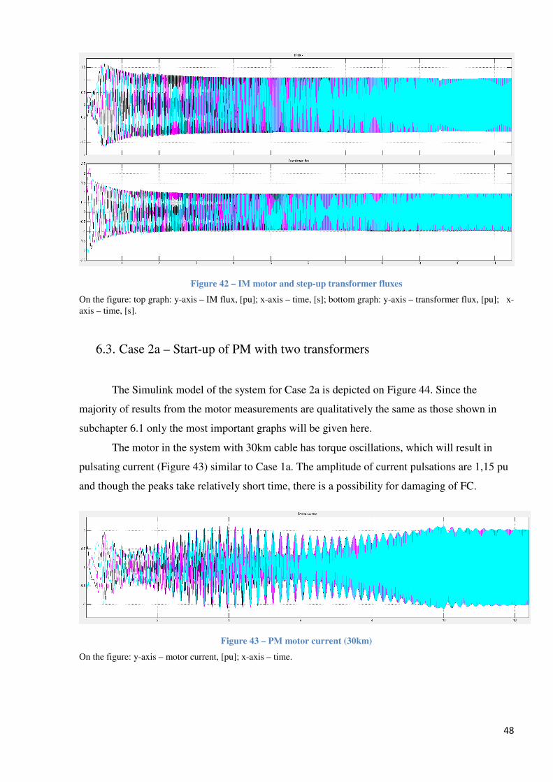
Figure 42 – IM motor and step-up transformer fluxes
On the figure: top graph: y-axis – IM flux, [pu]; x-axis – time, [s]; bottom graph: y-axis – transformer flux, [pu]; x-
axis – time, [s].
6.3. Case 2a – Start-up of PM with two transformers
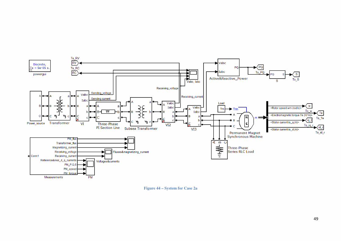
The Simulink model of the system for Case 2a is depicted on Figure 44. Since the
majority of results from the motor measurements are qualitatively the same as those shown in
subchapter 6.1 only the most important graphs will be given here.
The motor in the system with 30km cable has torque oscillations, which will result in
pulsating current (Figure 43) similar to Case 1a. The amplitude of current pulsations are 1,15 pu
and though the peaks take relatively short time, there is a possibility for damaging of FC.
Figure 43 – PM motor current (30km)
On the figure: y-axis – motor current, [pu]; x-axis – time.
49
Figure 44 – System for Case 2a
50
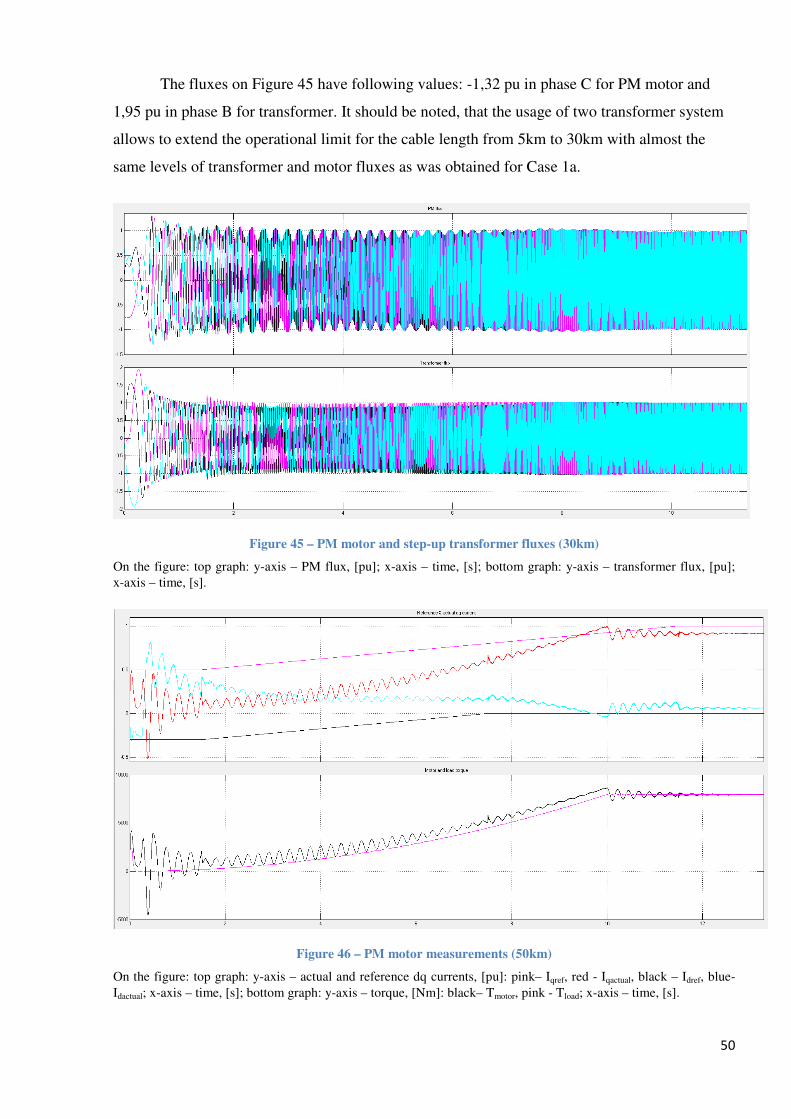
The fluxes on Figure 45 have following values: -1,32 pu in phase C for PM motor and
1,95 pu in phase B for transformer. It should be noted, that the usage of two transformer system
allows to extend the operational limit for the cable length from 5km to 30km with almost the
same levels of transformer and motor fluxes as was obtained for Case 1a.
Figure 45 – PM motor and step-up transformer fluxes (30km)
On the figure: top graph: y-axis – PM flux, [pu]; x-axis – time, [s]; bottom graph: y-axis – transformer flux, [pu];
x-axis – time, [s].
Figure 46 – PM motor measurements (50km)
On the figure: top graph: y-axis – actual and reference dq currents, [pu]: pink– Iqref, red - Iqactual, black – Idref, blue-
Idactual; x-axis – time, [s]; bottom graph: y-axis – torque, [Nm]: black– Tmotor, pink - Tload; x-axis – time, [s].
51
If the length increased to 50km, it can be observed that the torque oscillations (Figure 46)
became smaller than in the case with 30km cable. This is due to the increased resistance of the
cable, which plays a role of a damper in this case. The improvement in motor operation can be
also seen in the motor currents on Figure 47, which has no current pulsation.
Figure 47 – PM motor current (50km)
On the figure: y-axis – motor current, [pu]; x-axis – time.
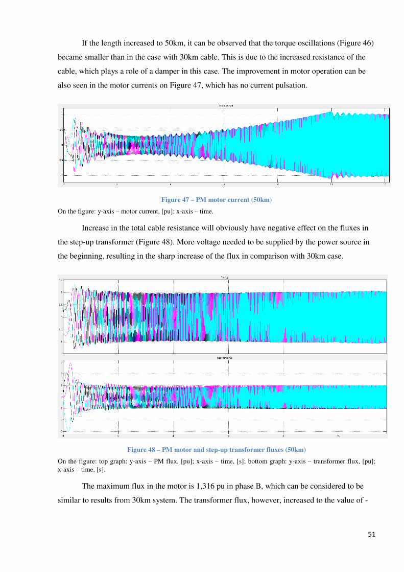
Increase in the total cable resistance will obviously have negative effect on the fluxes in
the step-up transformer (Figure 48). More voltage needed to be supplied by the power source in
the beginning, resulting in the sharp increase of the flux in comparison with 30km case.
Figure 48 – PM motor and step-up transformer fluxes (50km)
On the figure: top graph: y-axis – PM flux, [pu]; x-axis – time, [s]; bottom graph: y-axis – transformer flux, [pu];
x-axis – time, [s].
The maximum flux in the motor is 1,316 pu in phase B, which can be considered to be
similar to results from 30km system. The transformer flux, however, increased to the value of -
52
2,98 pu in phase C. Three times larger transformer core is required to avoid going into the
saturation region.
6.4. Case 2b – Start-up of IM with two transformers
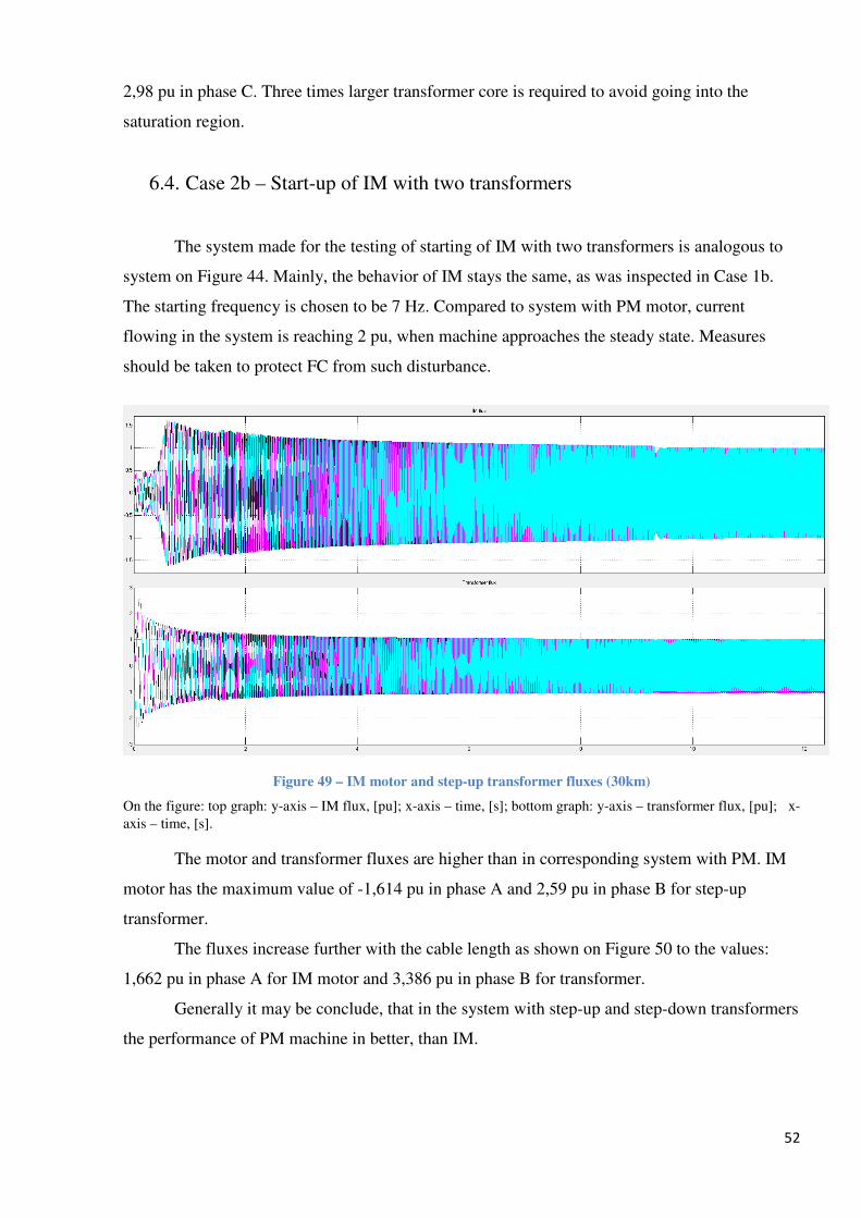
The system made for the testing of starting of IM with two transformers is analogous to
system on Figure 44. Mainly, the behavior of IM stays the same, as was inspected in Case 1b.
The starting frequency is chosen to be 7 Hz. Compared to system with PM motor, current
flowing in the system is reaching 2 pu, when machine approaches the steady state. Measures
should be taken to protect FC from such disturbance.
Figure 49 – IM motor and step-up transformer fluxes (30km)
On the figure: top graph: y-axis – IM flux, [pu]; x-axis – time, [s]; bottom graph: y-axis – transformer flux, [pu]; x-
axis – time, [s].
The motor and transformer fluxes are higher than in corresponding system with PM. IM
motor has the maximum value of -1,614 pu in phase A and 2,59 pu in phase B for step-up
transformer.
The fluxes increase further with the cable length as shown on Figure 50 to the values:
1,662 pu in phase A for IM motor and 3,386 pu in phase B for transformer.
Generally it may be conclude, that in the system with step-up and step-down transformers
the performance of PM machine in better, than IM.
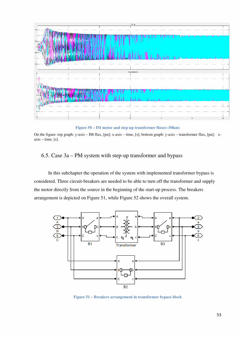
53
Figure 50 – IM motor and step-up transformer fluxes (50km)
On the figure: top graph: y-axis – IM flux, [pu]; x-axis – time, [s]; bottom graph: y-axis – transformer flux, [pu]; x-
axis – time, [s].
6.5. Case 3a – PM system with step-up transformer and bypass
In this subchapter the operation of the system with implemented transformer bypass is
considered. Three circuit-breakers are needed to be able to turn off the transformer and supply
the motor directly from the source in the beginning of the start-up process. The breakers
arrangement is depicted on Figure 51, while Figure 52 shows the overall system.
Figure 51 – Breakers arrangement in transformer bypass block
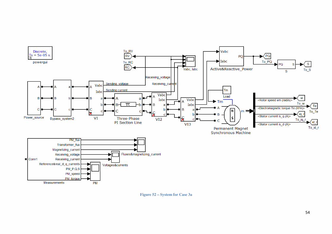
54
Figure 52 – System for Case 3a

55
Figure 53 – PM motor measurements
On the figure: 1st graph: y-axis – actual and reference dq currents, [pu]: pink– Iqref, red - Iqactual, black – Idref, blue-
Idactual; x-axis – time, [s];
2nd
graph: y-axis – motor power, [VA]: black– Pmotor, pink - Qmotor, blue – Smotor; x-axis – time, [s];
3rd
graph: y-axis – motor speed, [rad/s]; x-axis – time, [s].
4th
graph: y-axis – torque, [Nm]: black– Tmotor, pink - Tload; x-axis – time, [s].
Measurements on Figure 53 show successful start of the motor with transformer bypass.
The motor behaves in a way similar to the system in Case 1a without bypass. To reconnect the
transformer, first breaker B2 should open, following by closure of the breakers B1 and B3. The
opening of breaker B2 is done at t = 2,4615s when current in phase A is at zero crossing as
shown on Figure 54. The currents in other two phases are forced to go to zero as well. It should
be noted that no other breaker can operate before currents in all three phases are gone to zero.
The reconnection of transformer is performed at 2,4865s by closure of breaker B1. Since the
circuit is still broken no current will flow in the system until breaker B3 will close at t = 2,5115s.
The delay between breakers operations equal to 25ms is found to be enough for the stable
operation of the system.
From Figure 53 it is seen that at 12s the sudden load change occurs and the load
decreases by 20%. It can be seen that the system is able to reach a new steady state short after the
disturbance happened.
The DC offset caused by switching at different phase angles can saturate the transformer.
As was explained in Chapter 4, by pre-magnetizing the core to certain initial values of the flux,
the reduction of DC component is achieved. Figure 55 indicates that the flux in the transformer is
equal to 1pu and does not drive the core into saturation.
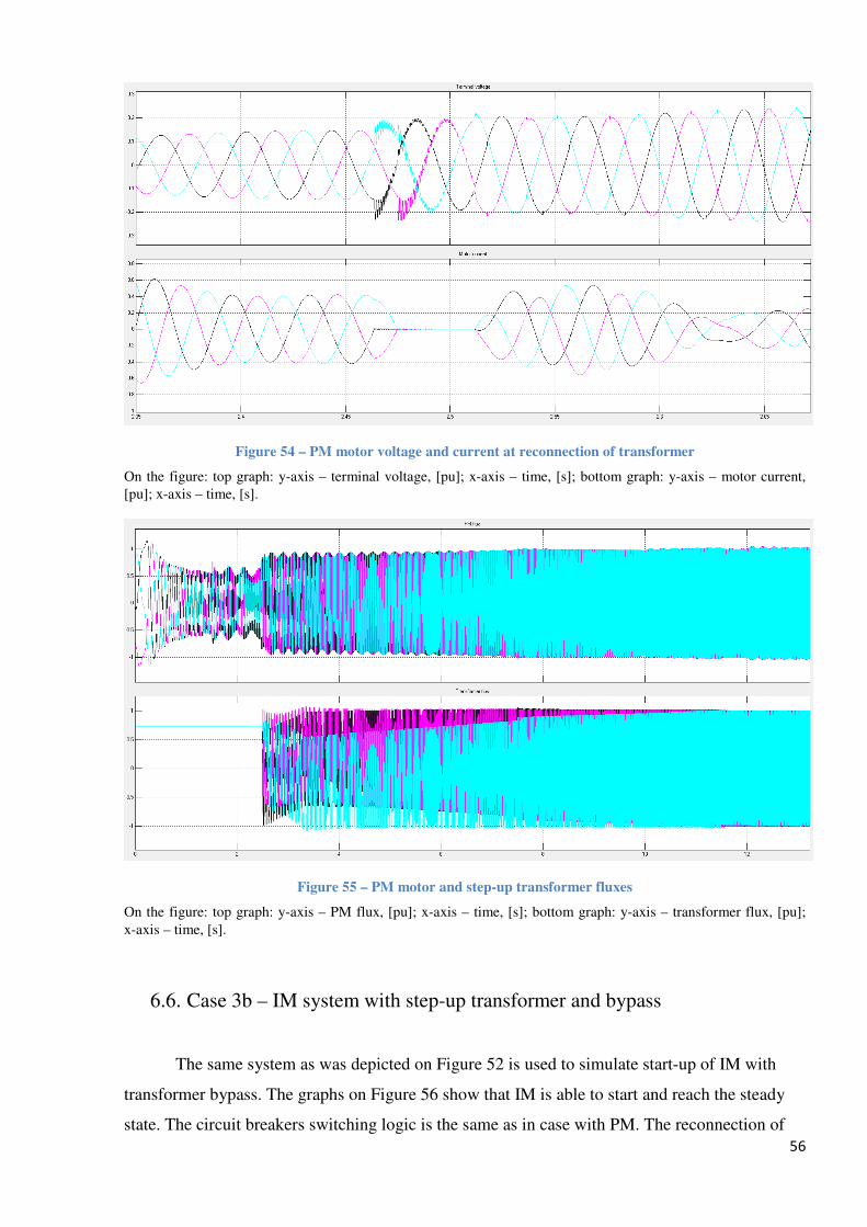
56
Figure 54 – PM motor voltage and current at reconnection of transformer
On the figure: top graph: y-axis – terminal voltage, [pu]; x-axis – time, [s]; bottom graph: y-axis – motor current,
[pu]; x-axis – time, [s].
Figure 55 – PM motor and step-up transformer fluxes
On the figure: top graph: y-axis – PM flux, [pu]; x-axis – time, [s]; bottom graph: y-axis – transformer flux, [pu];
x-axis – time, [s].
6.6. Case 3b – IM system with step-up transformer and bypass
The same system as was depicted on Figure 52 is used to simulate start-up of IM with
transformer bypass. The graphs on Figure 56 show that IM is able to start and reach the steady
state. The circuit breakers switching logic is the same as in case with PM. The reconnection of
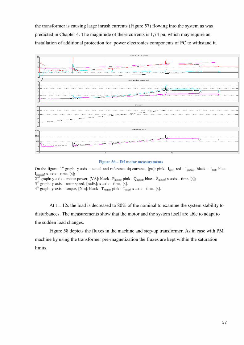
57
the transformer is causing large inrush currents (Figure 57) flowing into the system as was
predicted in Chapter 4. The magnitude of these currents is 1,74 pu, which may require an
installation of additional protection for power electronics components of FC to withstand it.
Figure 56 – IM motor measurements
On the figure: 1st graph: y-axis – actual and reference dq currents, [pu]: pink– Iqref, red - Iqactual, black – Idref, blue-
Idactual; x-axis – time, [s];
2nd
graph: y-axis – motor power, [VA]: black– Pmotor, pink - Qmotor, blue – Smotor; x-axis – time, [s];
3rd
graph: y-axis – rotor speed, [rad/s]; x-axis – time, [s].
4th
graph: y-axis – torque, [Nm]: black– Tmotor, pink - Tload; x-axis – time, [s].
At t = 12s the load is decreased to 80% of the nominal to examine the system stability to
disturbances. The measurements show that the motor and the system itself are able to adapt to
the sudden load changes.
Figure 58 depicts the fluxes in the machine and step-up transformer. As in case with PM
machine by using the transformer pre-magnetization the fluxes are kept within the saturation
limits.
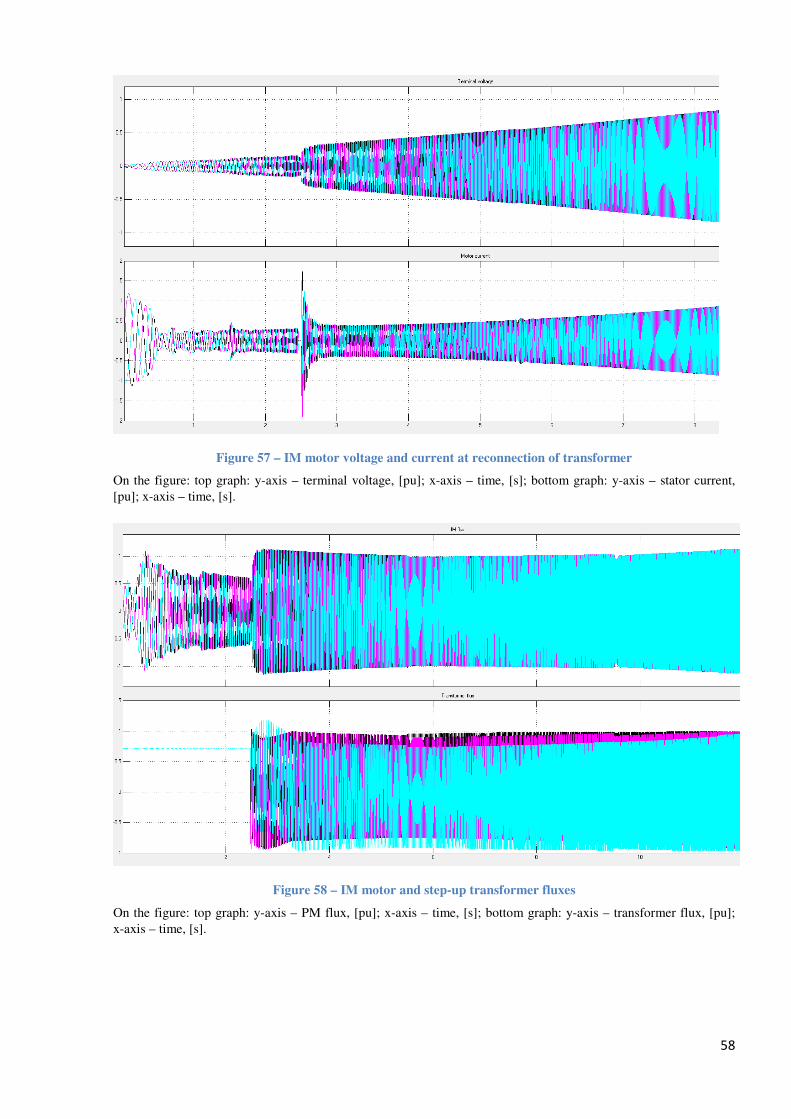
58
Figure 57 – IM motor voltage and current at reconnection of transformer
On the figure: top graph: y-axis – terminal voltage, [pu]; x-axis – time, [s]; bottom graph: y-axis – stator current,
[pu]; x-axis – time, [s].
Figure 58 – IM motor and step-up transformer fluxes
On the figure: top graph: y-axis – PM flux, [pu]; x-axis – time, [s]; bottom graph: y-axis – transformer flux, [pu];
x-axis – time, [s].
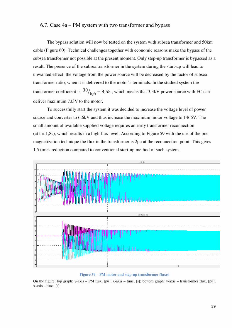
59
6.7. Case 4a – PM system with two transformer and bypass
The bypass solution will now be tested on the system with subsea transformer and 50km
cable (Figure 60). Technical challenges together with economic reasons make the bypass of the
subsea transformer not possible at the present moment. Only step-up transformer is bypassed as a
result. The presence of the subsea transformer in the system during the start-up will lead to
unwanted effect: the voltage from the power source will be decreased by the factor of subsea
transformer ratio, when it is delivered to the motor’s terminals. In the studied system the
transformer coefficient is 30 6,6y = 4,55, which means that 3,3kV power source with FC can
deliver maximum 733V to the motor.
To successfully start the system it was decided to increase the voltage level of power
source and converter to 6,6kV and thus increase the maximum motor voltage to 1466V. The
small amount of available supplied voltage requires an early transformer reconnection
(at t = 1,8s), which results in a high flux level. According to Figure 59 with the use of the pre-
magnetization technique the flux in the transformer is 2pu at the reconnection point. This gives
1,5 times reduction compared to conventional start-up method of such system.
Figure 59 – PM motor and step-up transformer fluxes
On the figure: top graph: y-axis – PM flux, [pu]; x-axis – time, [s]; bottom graph: y-axis – transformer flux, [pu];
x-axis – time, [s].
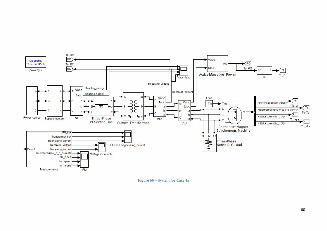
60
Figure 60 – System for Case 4a
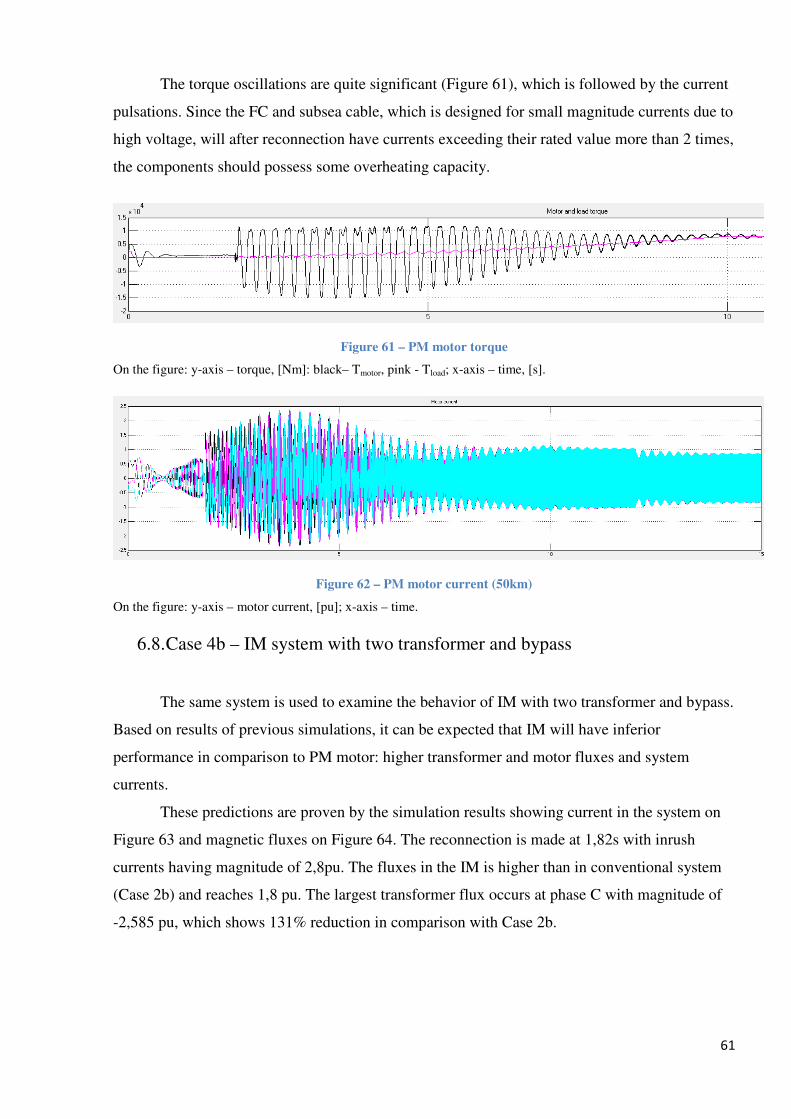
61
The torque oscillations are quite significant (Figure 61), which is followed by the current
pulsations. Since the FC and subsea cable, which is designed for small magnitude currents due to
high voltage, will after reconnection have currents exceeding their rated value more than 2 times,
the components should possess some overheating capacity.
Figure 61 – PM motor torque
On the figure: y-axis – torque, [Nm]: black– Tmotor, pink - Tload; x-axis – time, [s].
Figure 62 – PM motor current (50km)
On the figure: y-axis – motor current, [pu]; x-axis – time.
6.8. Case 4b – IM system with two transformer and bypass
The same system is used to examine the behavior of IM with two transformer and bypass.
Based on results of previous simulations, it can be expected that IM will have inferior
performance in comparison to PM motor: higher transformer and motor fluxes and system
currents.
These predictions are proven by the simulation results showing current in the system on
Figure 63 and magnetic fluxes on Figure 64. The reconnection is made at 1,82s with inrush
currents having magnitude of 2,8pu. The fluxes in the IM is higher than in conventional system
(Case 2b) and reaches 1,8 pu. The largest transformer flux occurs at phase C with magnitude of
-2,585 pu, which shows 131% reduction in comparison with Case 2b.
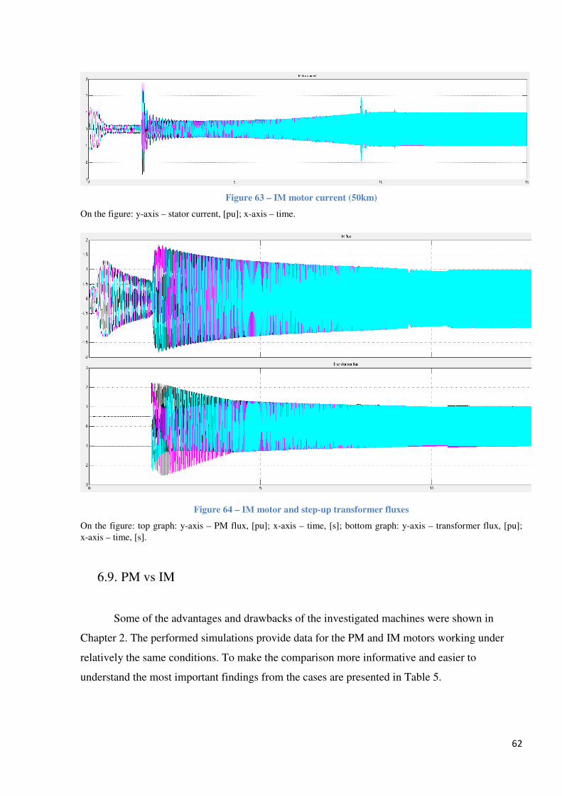
62
Figure 63 – IM motor current (50km)
On the figure: y-axis – stator current, [pu]; x-axis – time.
Figure 64 – IM motor and step-up transformer fluxes
On the figure: top graph: y-axis – PM flux, [pu]; x-axis – time, [s]; bottom graph: y-axis – transformer flux, [pu];
x-axis – time, [s].
6.9. PM vs IM
Some of the advantages and drawbacks of the investigated machines were shown in
Chapter 2. The performed simulations provide data for the PM and IM motors working under
relatively the same conditions. To make the comparison more informative and easier to
understand the most important findings from the cases are presented in Table 5.

63
Table 5 – Comparison between PM and IM
Case ���, [pu] ∆B c/0�;9, [pu]
PM
With step-up (5km) 1,1 significant 2,1
With subsea transformer 30km (50 km) 1,15 (1,1) significant
(moderate) 1,95 (2,98)
Step-up with bypass 1,1 significant 1
Subsea with bypass 50km 2,3 significant 2
Case ���, [pu] ∆B c/0�;9, [pu]
IM
With step-up (5km) 1,6 small 2,26
With subsea transformer 30km (50 km) 2 small 2,59 (3,386)
Step-up with bypass 1,74 small 1
Subsea with bypass 50km 2,8 small 2,585
where
���– maximum of the current flowing in the system,
∆B– motor torque oscillations,
c/0�;9– flux in the transformer.
As could be seen, the systems with PM machine have generally better performance than
with IM. The magnitudes of currents flowing in the system are lower, as well as magnetic flux in
the transformer. The lower values of the flux will require less degree of oversizing, which allows
to make the subsea system cheaper and will save free space on the platform. The only drawback
of PM motor is found to be the significantly oscillating torque. This causes the current pulsations
and fluctuations of the speed. The PM machine with implemented damper winding should be
able to improve the situation making the PM system absolutely superior than system with IM.
Such advantages as easier control and no need of the slip estimation techniques speak in
favor of the PM technology as well.

64
7. Conclusion
Two types of subsea motors were studied and simulated under current research:
permanent magnet synchronous motor and induction motor. PMSM has great potential for
replacing an IM in the subsea applications. Such advantages as absence of the rotor losses, lower
start-up currents and higher efficiency ensure the wide penetration of the permanent magnet
machines in the future [1].
The system which is capable of supplying power to the 5MW subsea motor was designed
with estimation and selection of the components parameters. The topology with only step-up
transformer greatly limits the system’s operational range and the maximum cable length due to
the voltage drop requirements. To extend the possible distance from the power source to the
motor an additional step-down (subsea) transformer need to be installed.
The maximum current flowing through the frequency converter and the magnetic flux of
the transformer are the main challenges during the start-up of the system. The power electronic
elements in the converter are not able to withstand high currents that can flow in the system and
therefore the currents should be limited. A high value of magnetic flux will drive transformer
into the saturation. In case of IM motor it was shown that the selection of initial starting
frequency represents a tradeoff between these two quantities: the lower the frequency the higher
the flux and lower the currents and vice versa.
The simulation model was built in order to show the conventional start-up of the IM and
PMSM with and without subsea transformer and to test the transformer bypass solution
suggested by SmartMotor AS.
With conventional start-up method, there is a large magnetic flux at the transformer,
which causes saturation of its core. In the system with 50km cable the flux can reach the
magnitude of more than 3 pu. This is in line with Aker Solutions results [31] with similar flux
levels for a long cable system. Transformer, therefore, must be oversized to avoid negative
effects on the system performance. Implemented control strategy used in the systems with PM
machine allows to limit the currents flowing in the system to the moderate levels.
The system with implemented bypass solution was proven to be able to successfully start
the motor and reduce the saturation problem. In the system with step-up transformer the flux was
reduced to the rated value and no oversizing is now necessary. However, the topology with two
transformers has additional obstacle due to the impossibility of bypassing the subsea transformer.
This can result in the necessity of using the power source and frequency converter designed for

65
the higher voltage levels to provide enough voltage to the motor. The early reconnection of the
transformer does not allow to fully eliminate the saturation problem, but only reduce it.
The decision of using the system with bypass transformer should be made on the grounds
of technical and economic analyses. To implement the transformer bypass, three circuit breakers
need to be installed. This leads to the increase of the costs of such systems, raising the question if
this is more beneficial than oversizing of the existing transformer. It was estimated that the
topology with bypass becomes economically feasible, when the required oversizing is 1,7 – 2
times.
However in case of a shortage of a free space on the platforms, bypass approach seems
more desirable, than increase of the transformer dimensions [1].
The sudden decrease of the load by 20% was simulated in the system with transformer
bypass. The system response to the change and ability to achieve a new steady state shows the
system robustness to such disturbances.

66
8. Future work
This section contains the suggestions for improvement and further development of work
done under the current research.
The operation and start-up of the PM machine need to be further investigated. The large
torque oscillations were observed as one of the drawbacks of such type of machine. Simulating
and analyzing of the dynamic behavior in the presence of the damper winding can be a next step
in reducing the oscillations magnitude [1].
An open loop controller model was made to control the motor start-up. A good match
was observed between the actual and reference values of the dq currents, when the system
reaches the steady state. However, in the very beginning of the starting procedure the actual
currents deviate from the reference quiet significantly. This can be improved by better controller
optimization. Another problem is supplying too much voltage right after the stiction torque was
overcome. This shows the need for some kind of indirect feedback to be able to adjust voltage
more precisely and thus reduce the maximum flux in the transformer and motor.
Controller used for simulations was made based on the PM machine equations and
applied to the systems with both PM and IM motors. Although, the IM is able to start and
achieve steady state, the performance of the IM motor can be improved by introducing a new
controller specially made for such a machine. This will require the estimation of the rotor speed
and the slip together with precise evaluation of IM parameters.
Some of the Simulink models for the power system components were proven to be
insufficient for a detailed analysis. The DC-component of the flux is not decaying if there is no
saturation in the transformer model. This does not correspond to the behavior of the transformer
in reality. In addition to that, it is not possible to simulate the transformer pre-magnetization in
the systems with bypass, since the flux in the model is defined as integral of the voltage. The
methods for overcoming these problems were implemented in the project, but a new realistic
model of the transformer needs to be made to improve the simulation results.
A transformer bypass in the system with step-up and subsea transformer should be
closely analyzed. There is a potential for further reduction of the transformer fluxes, by
optimizing the amount of the voltage supplied to the machine.
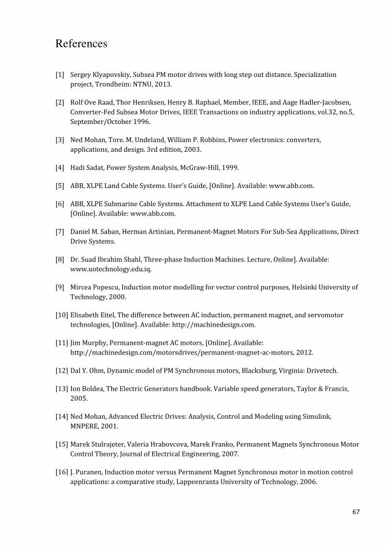
67
References
[1] Sergey Klyapovskiy, Subsea PM motor drives with long step out distance. Specialization
project, Trondheim: NTNU, 2013.
[2] Rolf Ove Raad, Thor Henriksen, Henry B. Raphael, Member, IEEE, and Aage Hadler-Jacobsen,
Converter-Fed Subsea Motor Drives, IEEE Transactions on industry applications, vol.32, no.5,
September/October 1996.
[3] Ned Mohan, Tore. M. Undeland, William P. Robbins, Power electronics: converters,
applications, and design. 3rd edition, 2003.
[4] Hadi Sadat, Power System Analysis, McGraw-Hill, 1999.
[5] ABB, XLPE Land Cable Systems. User’s Guide, [Online]. Available: www.abb.com.
[6] ABB, XLPE Submarine Cable Systems. Attachment to XLPE Land Cable Systems User’s Guide,
[Online]. Available: www.abb.com.
[7] Daniel M. Saban, Herman Artinian, Permanent-Magnet Motors For Sub-Sea Applications, Direct
Drive Systems.
[8] Dr. Suad Ibrahim Shahl, Three-phase Induction Machines. Lecture, Online]. Available:
www.uotechnology.edu.iq.
[9] Mircea Popescu, Induction motor modelling for vector control purposes, Helsinki University of
Technology, 2000.
[10] Elisabeth Eitel, The difference between AC induction, permanent magnet, and servomotor
technologies, [Online]. Available: http://machinedesign.com.
[11] Jim Murphy, Permanent-magnet AC motors, [Online]. Available:
http://machinedesign.com/motorsdrives/permanent-magnet-ac-motors, 2012.
[12] Dal Y. Ohm, Dynamic model of PM Synchronous motors, Blacksburg, Virginia: Drivetech.
[13] Ion Boldea, The Electric Generators handbook. Variable speed generators, Taylor & Francis,
2005.
[14] Ned Mohan, Advanced Electric Drives: Analysis, Control and Modeling using Simulink,
MNPERE, 2001.
[15] Marek Stulrajeter, Valeria Hrabovcova, Marek Franko, Permanent Magnets Synchronous Motor
Control Theory, Journal of Electrical Engineering, 2007.
[16] J. Puranen, Induction motor versus Permanent Magnet Synchronous motor in motion control
applications: a comparative study, Lappeenranta University of Technology, 2006.

68
[17] The MathWorks, Matlab/Simulink help: Per unit system.
[18] Delta-star or delta-y transformation simulation, [Online]. Available: http://www.cirvirlab.com,
2014.
[19] Trond Toftevaag, Mini project specification for the course “TET4200 Marine and offshore
power systems”,, Trondheim: NTNU, 2012.
[20] Ned Mohan, Electric Drives. An Integrative Approach, MNPERE, 2001.
[21] The Hysteresis Loop and Magnetic Properties, [Online]. Available: http://www.ndt-
ed.org/EducationResources.
[22] S.V. Kulkarni, S.A. Khaparde, Transformer Engineering. Design, Technology, and Diagnostics.
Second Edition, CRC Press, 2012.
[23] C. Sankaran, Effects of Harmonics on Power Systems, [Online]. Available:
http://ecmweb.com/power-quality/effects-harmonics-power-systems, 1999.
[24] Arne Nysveen, Subsea motor drives. Start-up of motor drives with long cable. Lecture
presentation, Trondheim: NTNU, 2012.
[25] Jerry R. Bednarczyk, P.E., Induction Motor Theory - PDHonline Course, [Online]. Available:
http://www.pdhonline.org/courses/e176.
[26] M. Jamali, M. Mirzaie, S. Asghar Gholamian, Calculation and Analysis of Transformer Inrush
Current Based on Parameters of Transformer and Operating Conditions, Electronics and
electrical engineering, ISSN 1392 - 1215, 2011.
[27] Inrush currents, [Online]. Available: http://www.ece.mtu.edu.
[28] Types of control systems, [Online]. Available:
http://instrumentationandcontrollers.blogspot.no.
[29] Open & Closed Loop Control System - Advantages & Disadvantages, [Online]. Available:
http://www.123mylist.com, 2012.
[30] Identification and Compensation of Torque Ripple in High-Precision Permanent Magnet Motor
Drives.
[31] Aker Solutions, Ulike pumpedrifter med ulike krav til kraftforsyning. IFEA Seminar: Offshore
og Subsea Kraftforsyning, Gardemoen, 2010.

69
Appendix A
%%% System impedances
Sb = 6.25e6; % [VA], assumed value
Vb1 = 3.3e3; % [V]
Vb2 = 6.6e3; % [V]
Zb1 = (Vb1)^2/Sb; % [Ohm]
Zb2 = (Vb2)^2/Sb % [Ohm]
Ib1 = Sb/[sqrt(3)*Vb1] % [A]
Ib2 = Sb/[sqrt(3)*Vb2] % [A]
f = 100; % [Hz]
psib = [Vb2*sqrt(2)]/[2*pi*f] % [Vs], base flux linkage
%% Step-up transformer
% Base values
Sbsut = 8e6; % [VA], assumed value
Vb1sut = 3.3e3; % [V]
Vb2sut = 6.6e3; % [V]
Zb1sut = (Vb1sut)^2/Sbsut; % [Ohm]
Zb2sut = (Vb2sut)^2/Sbsut; % [Ohm]
R1sut = 0.005; % [pu]
L1sut = 0.025; % [pu]
R1sutn = R1sut*(Zb1sut/Zb1); % [pu]
X1sutn = L1sut*(Zb1sut/Zb1); % [pu]
R2sut = 0.005;
L2sut = 0.025;
X2sut = L2sut;
Rmsut = 500; % [pu]
Lmsut = 500; % [pu]
Rmsutn = Rmsut*(Zb1sut/Zb1); % [pu]
Xmsutn = Lmsut*(Zb1sut/Zb1); % [pu]
SUT = [R1sutn R2sut Rmsutn; X1sutn X2sut Xmsutn];
printmat(SUT, 'Parameters_step_up_transformer_[pu]', 'Resistance
Reactance', 'Primary Secondary Magnetizing' )
%% Cable
% For 400 mm^2 XLPE cable
l = 5; %[km], cable length
Rc = 0.0470*l; % [Ohm]
Lc = 0.31e-3*l; % [H]
Cc = 0.59e-6*l; % [F]
Rcpu = Rc/Zb2; % [pu]
Xlcpu = [Lc*2*pi*f]/Zb2; % [pu]
Xccpu = [1/(2*pi*f*Cc)]/Zb2; % [pu]
C = [l; Rcpu; Xlcpu; Xccpu];
printmat(C, 'Parameters_cable_[pu]', 'Length Resistance Ind_reactance
Cap_reactance', '' )
%% Induction motor
s = 0.0055; % slip, assumed value
Vllim = 6.6e3; % [V]

70
R1im = 0.12; % [Ohm]
L1im = 1.2469e-3; % [H]
R2im = 0.0761; % [Ohm]
L2im = L1im;
Lmim = 0.035; % [H]
R1impu = R1im/Zb2; % [pu]
X1impu = [L1im*2*pi*f]/Zb2; % [pu]
R2impu = R2im/Zb2; % [pu]
X2impu = X1impu;
Xmimpu = [Lmim*2*pi*f]/Zb2; % [pu]
Z1im = [(R2im/s) + L1im*2*pi*f*i];
Z2im = (Z1im*Lmim*2*pi*f*i)/[Z1im + Lmim*2*pi*f*i];
Z3im = Z2im + [R1im + L1im*2*pi*f*i]
Z3impu = Z3im/Zb2
Rtot = R1impu + R2impu
Xtot = X1impu + X2impu
Sim = sqrt(3)*Vllim*[conj(Vllim/Z3im)] % [VA], apparent power of the
machine
Pim = real(Sim);
Qim = imag(Sim);
Angle = (cart2pol(Pim,Qim));
Angle_deg = radtodeg(Angle)
pf = cos(Angle) % power factor
IM = [R1impu R2impu 0; X1impu X2impu Xmimpu];
printmat(IM, 'Parameters_induction_motor_[pu]', 'Resistance
Reactance', 'Stator Rotor Magnetizing' )
%% Permanent magnet motor
Rpm = 0.02474; % [Ohm]
Lpm = 6.1e-3; % [H]
Ipm = 600*sqrt(2) % [A]
Ipmpu = Ipm/Ib2
Ebpm = 5262; % [V], back EMF
Vcpm = [Ebpm*sqrt(2)]/[6] % [V/krpm], voltage constant
psipm = [Ebpm*sqrt(2)]/[2*pi*f]
Rpmpu = Rpm/Zb2; % [pu]
Xpmpu = [Lpm*2*pi*f]/Zb2; % [pu]
Lpmpu = Lpm/[Zb2/[2*pi*f]]; % [pu], inductance of the PM motor
Ipmpu = Ipm/Ib2; % [pu]
PM = [Rpmpu; Xpmpu];
printmat(PM, 'Parameters_permanent_magnet_motor_[pu]', 'Resistance
Reactance', 'Stator' )
%%% Calculating of the equivalent impedances
ZTP = R1sutn + X1sutn*i; % [pu], primary side of the transformer
ZTM = [Rmsutn*Xmsutn*i]/[Rmsutn + Xmsutn*i]; % [pu], equivalent
impedance of the magnetizing branch
ZTS = R2sut + X2sut*i; % [pu], secondary side of the transformer
ZCC1 = -Xccpu*i; % [pu]
ZCS = Rcpu + Xlcpu*i % [pu], equivalent serial impedance of the cable
ZCC2 = ZCC1;

71
%% Delta - star transformation
ZR = ZCS + ZCC2 + ZCC1;
ZA = [ZCS*ZCC1]/ZR;
ZB = [ZCC1*ZCC2]/ZR;
ZC = [ZCS*ZCC2]/ZR;
ZATS = ZTS + ZA;
%% Star - delta transformation
ZD = ZATS*ZC + ZC*ZB + ZB*ZATS; % [pu], denominator for the s-d
transformation
ZAC = ZD/ZB;
ZAB = ZD/ZC;
ZBC = ZD/ZATS;
ZTMAB = [ZAB*ZTM]/[ZAB + ZTM];
%% Second delta - star transformation
ZR2 = ZTMAB + ZBC + ZAC;
ZA2 = [ZAC*ZTMAB]/ZR2;
ZB2 = [ZTMAB*ZBC]/ZR2;
ZC2 = [ZAC*ZBC]/ZR2;
ZA2TP = ZA2 + ZTP;
Zth = [ZA2TP*ZB2]/[ZA2TP + ZB2] + ZC2 % [pu], Thevenin impedance with
detailed model
Zeq = ZTP + ZTS + ZCS % [pu], Thevenin impedance with simplified
model
%% Comparison of impedance calculated with the use of detailed and
simplified models
DMR = real(Zth); % real part of Thevenin impedance with detailed model
DMI = imag(Zth); % imaginary part of Thevenin impedance with detailed
model
[ADM MDM]= (cart2pol(DMR,DMI)) % angle and magnitude of Thevenin
impedance with detailed model
SMR = real(Zeq); % real part of Thevenin impedance with simplified
model
SMI = imag(Zeq); % imaginary part of Thevenin impedance with
simplified model
[ASM MSM]= (cart2pol(SMR,SMI)) % angle and magnitude of Thevenin
impedance with simplified model
DC = [[MDM - MSM]/[(MDM + MSM)*0.5]]*100 % difference

72
Appendix B
%%% System impedances
Sb = 5.4e6; % [VA], assumed value
Vb1 = 6.6e3; % [V]
Vb2 = 30e3; % [V]
Vb3 = 6.6e3; % [V]
Zb1 = (Vb1)^2/Sb; % [Ohm]
Zb2 = (Vb2)^2/Sb; % [Ohm]
Zb3 = (Vb3)^2/Sb; % [Ohm]
Ib1 = Sb/[sqrt(3)*Vb1] % [A]
Ib2 = Sb/[sqrt(3)*Vb2] % [A]
Ib3 = Sb/[sqrt(3)*Vb3] % [A]
f = 100; % [Hz]
psib = [Vb3*sqrt(2)]/[2*pi*f] % [Vs], base flux linkage
%% Step-up transformer
% Base values
Sbsut = 8e6; % [VA], assumed value
Vb1sut = 3.3e3; % [V]
Vb2sut = 30e3; % [V]
Zb1sut = (Vb1sut)^2/Sbsut; % [Ohm]
Zb2sut = (Vb2sut)^2/Sbsut; % [Ohm]
R1sut = 0.005; % [pu]
L1sut = 0.025; % [pu]
R1sutn = R1sut*(Zb1sut/Zb1); % [pu]
X1sutn = L1sut*(Zb1sut/Zb1); % [pu]
R2sut = 0.005;
L2sut = 0.025;
X2sut = L2sut;
Rmsut = 500; % [pu]
Lmsut = 500; % [pu]
Rmsutn = Rmsut*(Zb1sut/Zb1); % [pu]
Xmsutn = Lmsut*(Zb1sut/Zb1); % [pu]
SUT = [R1sutn R2sut Rmsutn; X1sutn X2sut Xmsutn];
printmat(SUT, 'Parameters_step_up_transformer_[pu]', 'Resistance
Reactance', 'Primary Secondary Magnetizing' )
%% Cable
% For 400 mm^2 XLPE cable
l = 50; %[km], cable length
Rc = 0.193*l; % [Ohm]
Lc = 0.44e-3*l; % [H]
Cc = 0.18e-6*l; % [F]
Rcpu = Rc/Zb2; % [pu]
Xlcpu = [Lc*2*pi*f]/Zb2; % [pu]
Xccpu = [1/(2*pi*f*Cc)]/Zb2; % [pu]
C = [l; Rcpu; Xlcpu; Xccpu];
printmat(C, 'Parameters_cable_[pu]', 'Length Resistance Ind_reactance
Cap_reactance', '' )
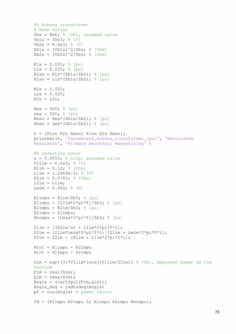
73
%% Subsea transformer
% Base values
Sbs = 8e6; % [VA], assumed value
Vb1s = 30e3; % [V]
Vb2s = 6.6e3; % [V]
Zb1s = (Vb1s)^2/Sbs; % [Ohm]
Zb2s = (Vb2s)^2/Sbs; % [Ohm]
R1s = 0.005; % [pu]
L1s = 0.025; % [pu]
R1sn = R1s*(Zb1s/Zb2); % [pu]
X1sn = L1s*(Zb1s/Zb2); % [pu]
R2s = 0.005;
L2s = 0.025;
X2s = L2s;
Rms = 500; % [pu]
Lms = 500; % [pu]
Rmsn = Rms*(Zb1s/Zb2); % [pu]
Xmsn = Lms*(Zb1s/Zb2); % [pu]
S = [R1sn R2s Rmsn; X1sn X2s Xmsn];
printmat(S, 'Parameters_subsea_transformer_[pu]', 'Resistance
Reactance', 'Primary Secondary Magnetizing' )
%% Induction motor
s = 0.0055; % slip, assumed value
Vllim = 6.6e3; % [V]
R1im = 0.12; % [Ohm]
L1im = 1.2469e-3; % [H]
R2im = 0.0783; % [Ohm]
L2im = L1im;
Lmim = 0.062; % [H]
R1impu = R1im/Zb3; % [pu]
X1impu = [L1im*2*pi*f]/Zb3; % [pu]
R2impu = R2im/Zb3; % [pu]
X2impu = X1impu;
Xmimpu = [Lmim*2*pi*f]/Zb3; % [pu]
Z1im = [(R2im/s) + L1im*2*pi*f*i];
Z2im = (Z1im*Lmim*2*pi*f*i)/[Z1im + Lmim*2*pi*f*i];
Z3im = Z2im + [R1im + L1im*2*pi*f*i];
Rtot = R1impu + R2impu
Xtot = X1impu + X2impu
Sim = sqrt(3)*Vllim*[conj(Vllim/Z3im)] % [VA], apparent power of the
machine
Pim = real(Sim);
Qim = imag(Sim);
Angle = (cart2pol(Pim,Qim));
Angle_deg = radtodeg(Angle)
pf = cos(Angle) % power factor
IM = [R1impu R2impu 0; X1impu X2impu Xmimpu];

74
printmat(IM, 'Parameters_induction_motor_[pu]', 'Resistance
Reactance', 'Stator Rotor Magnetizing' )
%% Permanent magnet motor
Rpm = 0.02474; % [Ohm]
Lpm = 6.1e-3; % [H]
Ipm = 600*sqrt(2); % [A]
Ipmpu = Ipm/Ib3
Ebpm = 5262; % [V], back EMF
Vcpm = [Ebpm*sqrt(2)]/[6] % [V/krpm], voltage constant
psipm = [Ebpm*sqrt(2)]/[2*pi*f]
Rpmpu = Rpm/Zb3; % [pu]
Xpmpu = [Lpm*2*pi*f]/Zb3; % [pu]
Lpmpu = Lpm/[Zb3/[2*pi*f]]; % [pu], inductance of the PM motor
Ipmpu = Ipm/Ib3; % [pu]
PM = [Rpmpu; Xpmpu];
printmat(PM, 'Parameters_permanent_magnet_motor_[pu]', 'Resistance
Reactance', 'Stator' )
%%% Calculating of the equivalent impedances
ZTP = R1sutn + X1sutn*i; % [pu], primary side of the transformer
ZTM = [Rmsutn*Xmsutn*i]/[Rmsutn + Xmsutn*i]; % [pu], equivalent
impedance of the magnetizing branch
ZTS = R2sut + X2sut*i; % [pu], secondary side of the transformer
ZCC1 = -Xccpu*i; % [pu]
ZCS = Rcpu + Xlcpu*i; % [pu], equivalent serial impedance of the cable
ZCC2 = ZCC1;
ZSTP = R1sn + X1sn*i; % [pu], primary side of the subsea transformer
ZSTM = [Rmsn*Xmsn*i]/[Rmsn + Xmsn*i]; % [pu], equivalent impedance of
the magnetizing branch
ZSTS = R2s + X2s*i; % [pu], secondary side of the subsea transformer
%% Delta - star transformation
ZR = ZCS + ZCC2 + ZCC1;
ZA = [ZCS*ZCC1]/ZR;
ZB = [ZCC1*ZCC2]/ZR;
ZC = [ZCS*ZCC2]/ZR;
ZATS = ZTS + ZA;
%% Star - delta transformation
ZD = ZATS*ZC + ZC*ZB + ZB*ZATS; % [pu], denominator for the s-d
transformation
ZAC = ZD/ZB;
ZAB = ZD/ZC;
ZBC = ZD/ZATS;
ZTMAB = [ZAB*ZTM]/[ZAB + ZTM];
%% Second delta - star transformation
ZR2 = ZTMAB + ZBC + ZAC;
ZA2 = [ZAC*ZTMAB]/ZR2;
ZB2 = [ZTMAB*ZBC]/ZR2;
ZC2 = [ZAC*ZBC]/ZR2;

75
ZA2TP = ZA2 + ZTP;
%% Second star - delta transformation
ZC2STP = ZC2 + ZSTP;
ZD2 = ZC2STP*ZSTS + ZC2STP*ZSTM + ZSTS*ZSTM; % [pu], denominator for
the s-d transformation
ZA1C = ZD2/ZSTM;
ZA1B = ZD2/ZSTS;
ZB1C = ZD2/ZC2STP;
ZB2A1B = [ZB2*ZA1B]/[ZB2 + ZA1B];
%% Third delta - star transformation
ZR3 = ZA1C + ZB2A1B + ZB1C;
ZA11 = [ZA1C*ZB2A1B]/ZR3;
ZB11 = [ZB2A1B*ZB1C]/ZR3;
ZC11 = [ZA1C*ZB1C]/ZR3;
ZA112TP = ZA2TP + ZA11;
Zth = [ZA112TP*ZB11]/[ZA112TP + ZB11] + ZC11 % [pu], Thevenin
impedance
Zeq = ZTP + ZTS + ZCS + ZSTP + ZSTS % [pu], Thevenin impedance with
simplified model
%% Comparison of impedance calculated with the use of detailed and
simplified models
DMR = real(Zth); % real part of Thevenin impedance with detailed model
DMI = imag(Zth); % imaginary part of Thevenin impedance with detailed
model
[ADM MDM]= (cart2pol(DMR,DMI)) % angle and magnitude of Thevenin
impedance with detailed model
SMR = real(Zeq); % real part of Thevenin impedance with simplified
model
SMI = imag(Zeq); % imaginary part of Thevenin impedance with
simplified model
[ASM MSM]= (cart2pol(SMR,SMI)) % angle and magnitude of Thevenin
impedance with simplified model
DC = [[MDM - MSM]/[(MDM + MSM)*0.5]]*100 % difference

76
Appendix C
%% Initial parameters
fn = 100; % [Hz], nominal frequency
f = 0:1:100; % [Hz] starting frequency
fratio = f/fn % frequency ratio
Vtn = 6.6e3; % [V], line-to-line voltage after transformer, base
voltage
Vb = 6.6e3; % [V], base voltage
Vtnph = Vtn/sqrt(3); % [V], line-to-neutral voltage after transformer
Vpu = [Vtnph*sqrt(3)]/Vb; % [pu]
%% Components parameters
% Transmission system
Zc = 0.0428 + 1i*0.1847 % [pu], impedance of transmission system
Zcs = 0.0942 + 1i*0.1792 % [pu], impedance of transmission system
% Induction motor
p = 2; % numbers of machine poles
Tstpu = 0.3; % [pu], stiction torque
Rspu = 0.01722; % [pu], stator resistance
Rrpu = 0.01092; % [pu], rotor resistance
Xspu = 0.11241; % [pu], stator reactance
Xlrpu = 0.11241; % [pu], rotor reactance
Xm = 3.15530; % [pu], magnetizing reactance
Zs = Rspu + 1i*Xspu; % [pu], stator impedance
%% Thevenin equivalent
Zth = [(Zs + Zc).*(1i*Xm)]./[Zs + Zc + 1i*Xm] % [pu], Thevenin
impedance
Rth = real(Zth);
Xth = imag(Zth);
Re = (Rth + Rrpu);
Xe = (Xth + Xlrpu);
Flux = sqrt([2*Tstpu*(Re.^2+ Xe.^2)]./[3*p*Rrpu*[2.*pi.*fratio]])
Ir = sqrt([Tstpu*2*pi.*fratio]/[3*Rrpu]) % [pu], current at stiction
torque
plot(f, Flux,'b', f, Ir,'g', 'LineWidth',2);
grid on
title('Flux and current curves')
ylabel('Flux [pu] / Current [pu]')
hleg1 = legend('Flux vs frequency','Current vs frequency');