Subject ECONOMICS Paper No and Title 1: Quantitative

____________________________________________________________________________________________________

Economics

Paper 1: Quantitative Methods- I (Mathematical Methods)

Module 33: Linear Programming- Introduction to Simplex Methods

1

Subject ECONOMICS

Paper No and Title 1: Quantitative Methods- I (Mathematical Methods)

Module No and Title 33: Linear Programming- Introduction to Simplex Methods

Module Tag ECO_P1_M33

____________________________________________________________________________________________________

Economics



2

TABLE OF CONTENTS

1. Learning Outcomes

2. Introduction

3. Solution of the linear programming problem by simplex method

Step 1: Standard form of a maximum problem

Step 2: Adding Slack variables and starting

Step 3: Forming simplex table

Step 4: Pivoting

Finding the pivot element

Applying smallest Quotient rule

4. Flowchart explaining Simplex Method

5. Summary

____________________________________________________________________________________________________

Economics



3

1. Learning Outcomes

After studying this module, you shall be able to:

Understand Simplex Method

When to use Simplex Method

Define slack variables

Prepare the linear programming problems problem in order to solve it by pivoting using

Simplex method

Solve the linear programming problems using simplex method

2. Introduction

In the previous lesson, we have solved linear programming problems by graphical method. This

method is useful when there are not more than two variables and the number of constraints is less

as it is easier to deal with two-dimensional graph. All the feasible solutions lie within the feasible

area on the graph and the corner points are tested for optimal solution. However, if we have large

number of variables or constraints, it is still true that the optimal solution will be found at the

vertex of the set of feasible solutions. In fact, we could find these vertices by writing all the

equations corresponding to the inequalities of the problem and then proceeding to solve all

possible combinations of these equations. Then, we could evaluate the objective function at the

feasible solutions. After all this, we might discover that the problem has no optimal solution at

all. Therefore, this method would be highly cumbersome and time consuming.

Suppose there are 4 variables and 7 constraints, we would have to solve all possible

combinations of 4 equations chosen from a set of 7 equations. Obviously, there would be

𝐶47 = (

74) = 35 solutions in all. Each of these solutions will then have to be tested for

feasibility. So even for this relatively small number of variables and constraints, the work would

be quite tedious.

____________________________________________________________________________________________________

Economics



4

One very efficient technique of solving these kinds of optimization problems with large number

of variables and constraints is Simplex method. The Simplex Method or simplex algorithm is

matrix-based method used for solving linear programming problems with any number of

variables. It is a method developed by George B. Dantzig, an American

mathematician, in 1947. The simplex method is an iterative procedure, solving a system of linear

equations in each of its steps, and stopping when either the optimum is reached or the solution

proves infeasible.

3. Solution of Linear Programming Problems by Simplex method

The procedure for solving the given problem is illustrated with the help of an example in the

following steps:

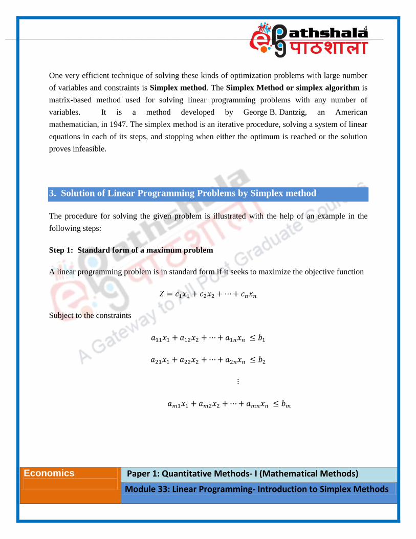
Step 1: Standard form of a maximum problem

A linear programming problem is in standard form if it seeks to maximize the objective function

𝑍 = 𝑐1𝑥1 + 𝑐2𝑥2 + ⋯+ 𝑐𝑛𝑥𝑛

Subject to the constraints

𝑎11𝑥1 + 𝑎12𝑥2 + ⋯+ 𝑎1𝑛𝑥𝑛 ≤ 𝑏1

𝑎21𝑥1 + 𝑎22𝑥2 + ⋯+ 𝑎2𝑛𝑥𝑛 ≤ 𝑏2

⋮

𝑎𝑚1𝑥1 + 𝑎𝑚2𝑥2 + ⋯+ 𝑎𝑚𝑛𝑥𝑛 ≤ 𝑏𝑚

____________________________________________________________________________________________________

Economics



5

The conditions required for a linear programming problem to be in standard form are:

i. All the variables are non–negative i.e 𝑥𝑖 ≥ 0.

ii. All the constraints and objective function, which is to be optimized, are written as a linear

expression. Also note that for a linear programming problem in standard form, the

objective function is to be maximized, not minimized.

iii. The right hand side of the constraints is positive or equal to zero i.e. 𝑏𝑖 ≥ 0. If the right

hand side of the constraint is negative then it must be made positive by multiplying both

sides of the equation by ‘-1’.

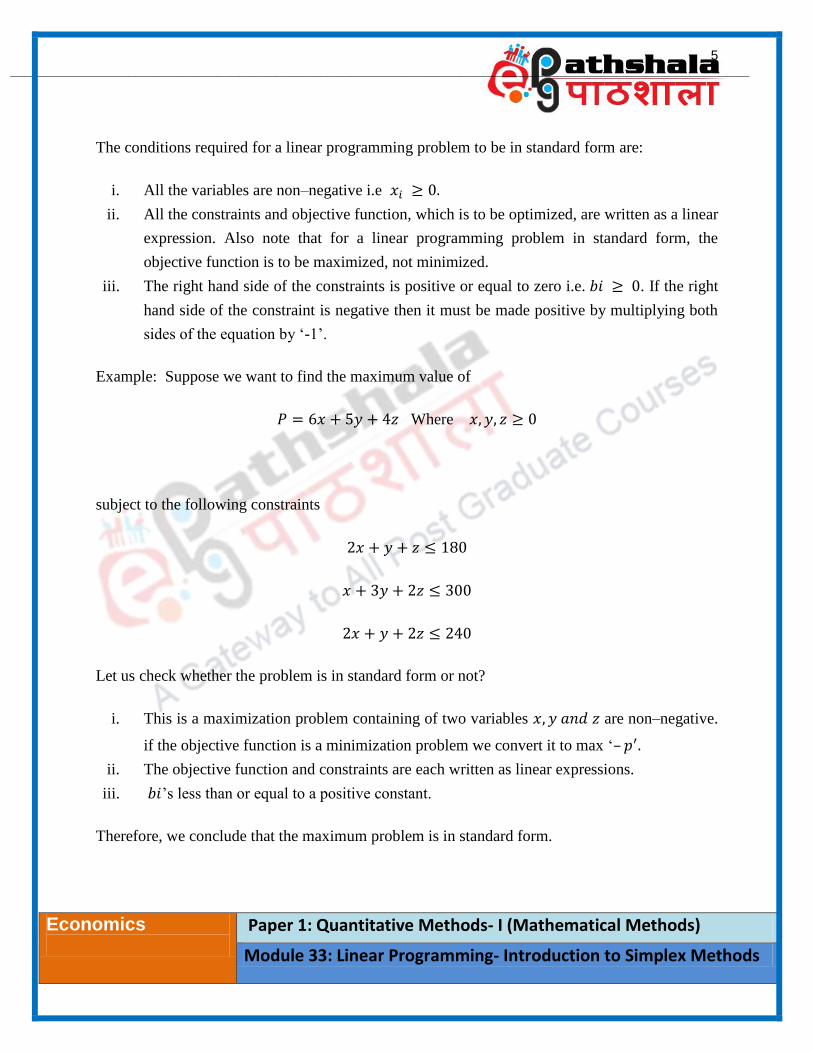
Example: Suppose we want to find the maximum value of

𝑃 = 6𝑥 + 5𝑦 + 4𝑧 Where 𝑥, 𝑦, 𝑧 ≥ 0

subject to the following constraints

2𝑥 + 𝑦 + 𝑧 ≤ 180

𝑥 + 3𝑦 + 2𝑧 ≤ 300

2𝑥 + 𝑦 + 2𝑧 ≤ 240

Let us check whether the problem is in standard form or not?

i. This is a maximization problem containing of two variables 𝑥, 𝑦 𝑎𝑛𝑑 𝑧 are non–negative.

if the objective function is a minimization problem we convert it to max ‘– 𝑝′.

ii. The objective function and constraints are each written as linear expressions.

iii. 𝑏𝑖’s less than or equal to a positive constant.

Therefore, we conclude that the maximum problem is in standard form.

____________________________________________________________________________________________________

Economics



6

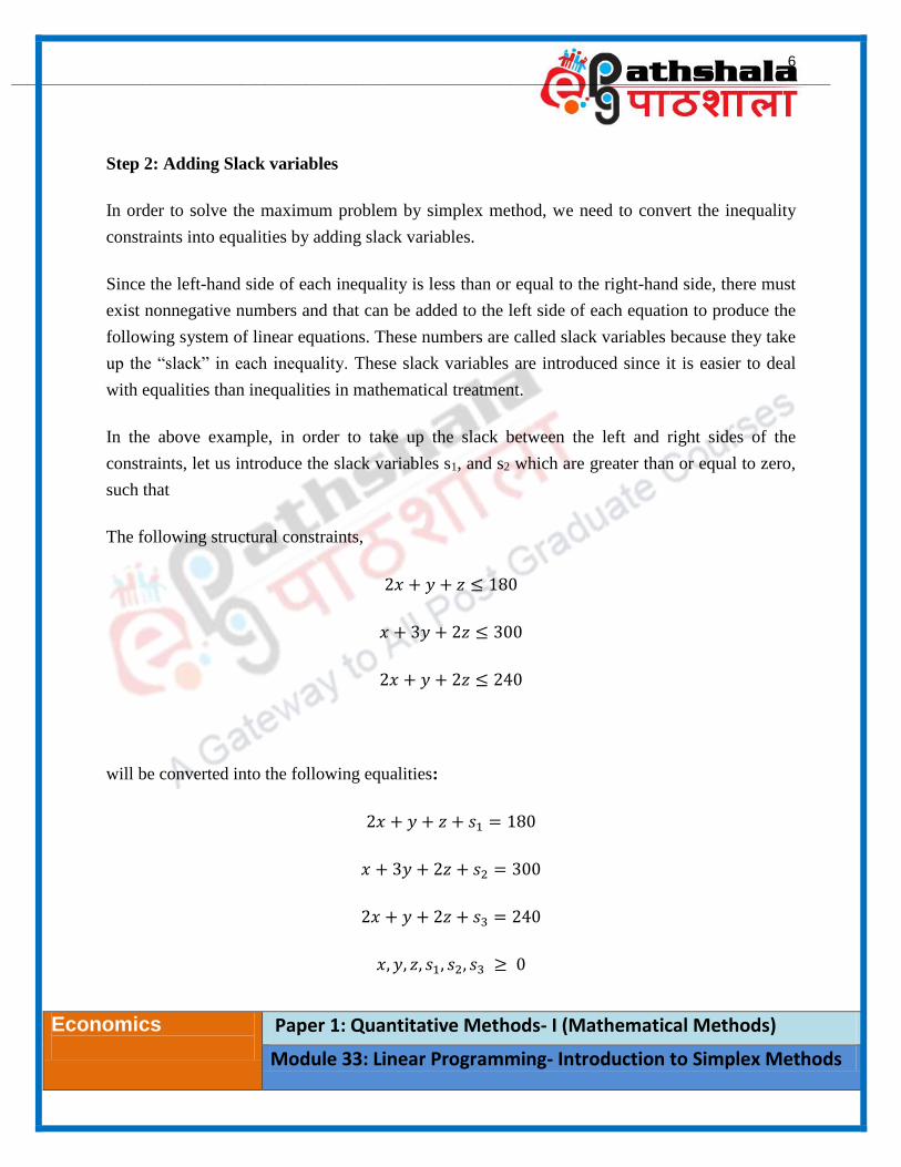
Step 2: Adding Slack variables

In order to solve the maximum problem by simplex method, we need to convert the inequality

constraints into equalities by adding slack variables.

Since the left-hand side of each inequality is less than or equal to the right-hand side, there must

exist nonnegative numbers and that can be added to the left side of each equation to produce the

following system of linear equations. These numbers are called slack variables because they take

up the “slack” in each inequality. These slack variables are introduced since it is easier to deal

with equalities than inequalities in mathematical treatment.

In the above example, in order to take up the slack between the left and right sides of the

constraints, let us introduce the slack variables s1, and s2 which are greater than or equal to zero,

such that

The following structural constraints,

2𝑥 + 𝑦 + 𝑧 ≤ 180

𝑥 + 3𝑦 + 2𝑧 ≤ 300

2𝑥 + 𝑦 + 2𝑧 ≤ 240

will be converted into the following equalities:

2𝑥 + 𝑦 + 𝑧 + 𝑠1 = 180

𝑥 + 3𝑦 + 2𝑧 + 𝑠2 = 300

2𝑥 + 𝑦 + 2𝑧 + 𝑠3 = 240

𝑥, 𝑦, 𝑧, 𝑠1, 𝑠2, 𝑠3 ≥ 0

____________________________________________________________________________________________________

Economics



7

The objective function becomes

−6𝑥 − 5𝑦 − 4𝑧 + 0𝑠1 + 0𝑠2 + 0𝑠3 + 𝑝 = 0

The slack variables will always be nonnegative (zero or positive) when solving linear

programming problem.

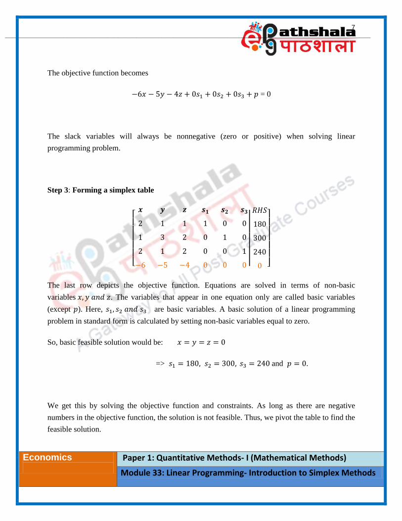
Step 3: Forming a simplex table

[

𝒙 𝒚 𝒛 𝒔𝟏 𝒔𝟐 𝒔𝟑

2 1 1 1 0 0

1 3 2 0 1 0

2 1 2 0 0 1

−6 −5 −4 0 0 0

|

|

𝑅𝐻𝑆

180

300

240

0 ]

The last row depicts the objective function. Equations are solved in terms of non-basic

variables 𝑥, 𝑦 𝑎𝑛𝑑 𝑧. The variables that appear in one equation only are called basic variables

(except 𝑝). Here, 𝑠1, 𝑠2 𝑎𝑛𝑑 𝑠3 are basic variables. A basic solution of a linear programming

problem in standard form is calculated by setting non-basic variables equal to zero.

So, basic feasible solution would be: 𝑥 = 𝑦 = 𝑧 = 0

=> 𝑠1 = 180, 𝑠2 = 300, 𝑠3 = 240 and 𝑝 = 0.

We get this by solving the objective function and constraints. As long as there are negative

numbers in the objective function, the solution is not feasible. Thus, we pivot the table to find the

feasible solution.

____________________________________________________________________________________________________

Economics



8

Step 4: Pivoting the simplex table

What is Pivoting?

Pivoting means to pivot a matrix about a given element, called the pivot element, is to apply row

operations so that the pivot element is replaced by 1 and all other entries in the same column

(called pivot column) becomes 0. More specifically, in the pivot row, divide each entry by the

pivot element (we assume it is not 0). Obtain 0 elsewhere in the pivot column by performing row

operations.

How is the pivot element selected?

First we find the pivot element: The column with the highest negative number in the objective

function, is chosen, which is column 1 here as the highest negative number is−6. Divide each

constant to the right hand side of the bar with the corresponding (non-zero) element in the pivot

column.

180/2 = 90

300/1 = 300

240/2 = 120

How to apply Smallest Quotient Rule?

Select the smallest quotient. The pivot element is the intersection of the column with the most

negative indicator and the row with the smallest quotient. The pivot is the ′2′ in column 1 in this

table. Now, Change the pivot element to 1. We can do this by

𝑅1 = ½ 𝑅1

____________________________________________________________________________________________________

Economics



9

[

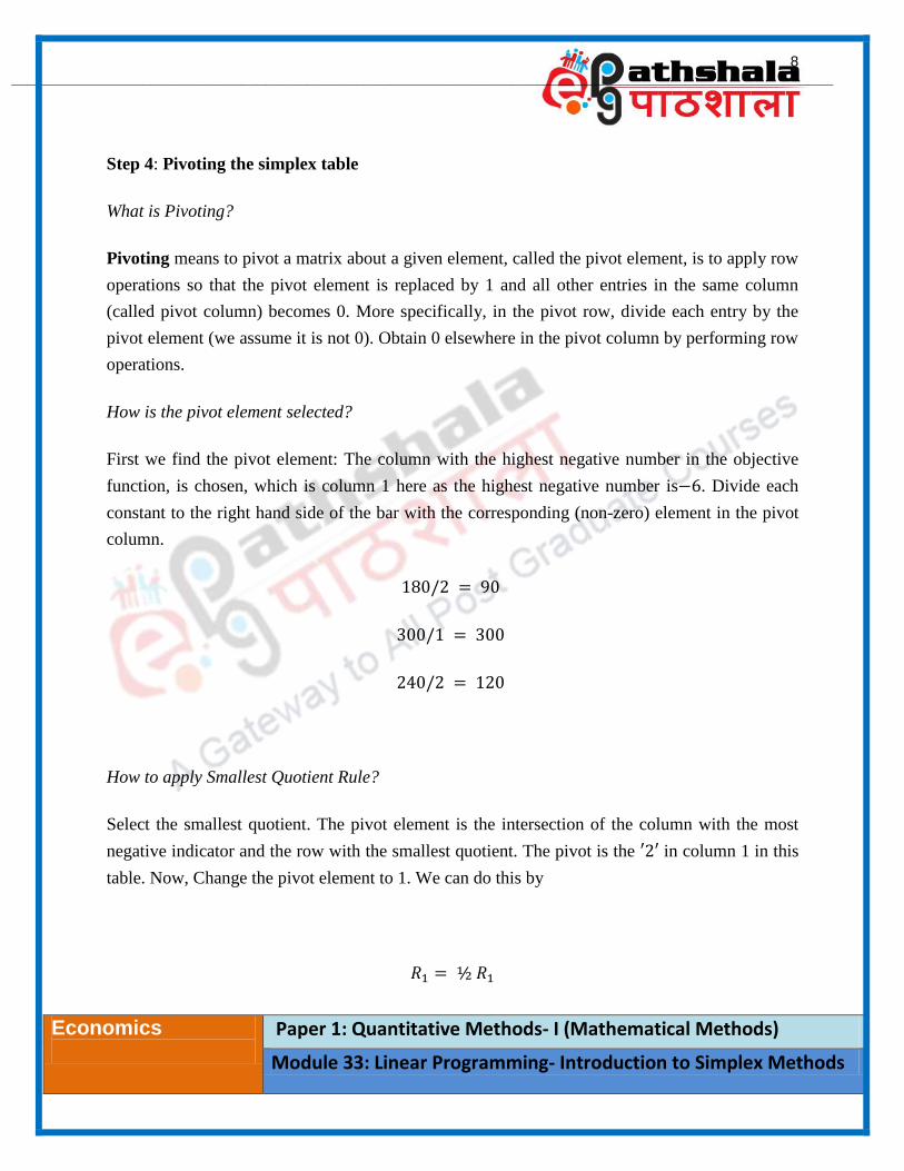
𝒙 𝒚 𝒛 𝒔𝟏 𝒔𝟐 𝒔𝟑

1 1/2 1/2 1/2 0 0

1 3 2 0 1 0

2 1 2 0 0 1

−6 −5 −4 0 0 0

|

|

𝑅𝐻𝑆

90

300

240

0 ]

Now, we Pivot about the pivot element to make other elements in the column equal to zero:

𝑅2 = − 𝑅1 + 𝑅2

𝑅3 = −2 𝑅1 + 𝑅3

𝑅4 = 6 𝑅1 + 𝑅4

[ 𝒙 𝒚 𝒛 𝒔𝟏 𝒔𝟐 𝒔𝟑

1 ½ ½ ½ 0 0

0 2 ½ 1 ½ −½ 1 0

0 0 1 −1 0 1

0 −2 −1 3 0 0

|

|

𝑅𝐻𝑆

90

210

60

540 ]

When pivoting is done, and we set the non-basic variables to zero, we obtain a solution called a

basic feasible solution to the linear programming problem.

The basic feasible solution from this tableau is 𝑥 = 90, 𝑠2 = 210, 𝑠3 = 60 𝑎𝑛𝑑 𝑦 = 0, 𝑧 =

0, 𝑠1 = 0 𝑎𝑛𝑑 𝑝 = 540. However; even this is not optimal as there are negative elements in last

row.

If a negative indicator is still present, we keep on pivoting. On the other hand, if no negative

indicators are present, the maximum of the objective function has been reached.

____________________________________________________________________________________________________

Economics



10

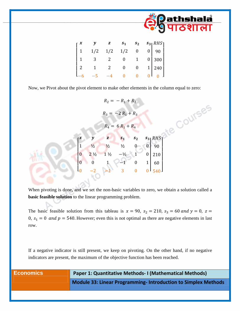
Step 5: Pivoting again:

Determine a new pivot element. Select the column with the most negative indicator: it is column

2 in this table. Divide each constant to the right of the bar by the corresponding (nonzero)

element in the pivot column.

90 ÷ ½ = 180

210 ÷ 2½ = 84

Select the smallest quotient which is 84. The pivot element is the intersection of the column with

the most negative indicator and the row with the smallest quotient. The pivot is the 2½ in

column 2 in this table.

Now, Change the pivot element to 1. We can do this by

𝑅2 = 𝑅2 ÷ 2½

[ 𝒙 𝒚 𝒛 𝒔𝟏 𝒔𝟐 𝒔𝟑

1 1/2 1/2 1/2 0 0

0 1 0.6 −0.2 0.4 0

0 0 1 −1 0 1

0 −2 −1 3 0 0

|

|

𝑅𝐻𝑆

90

84

60

540 ]

Now, we Pivot about the pivot element to make other elements in the column equal to zero:

𝑅1 = −0.5 𝑅2 + 𝑅1

𝑅4 = 2 𝑅2 + 𝑅4

____________________________________________________________________________________________________

Economics



11

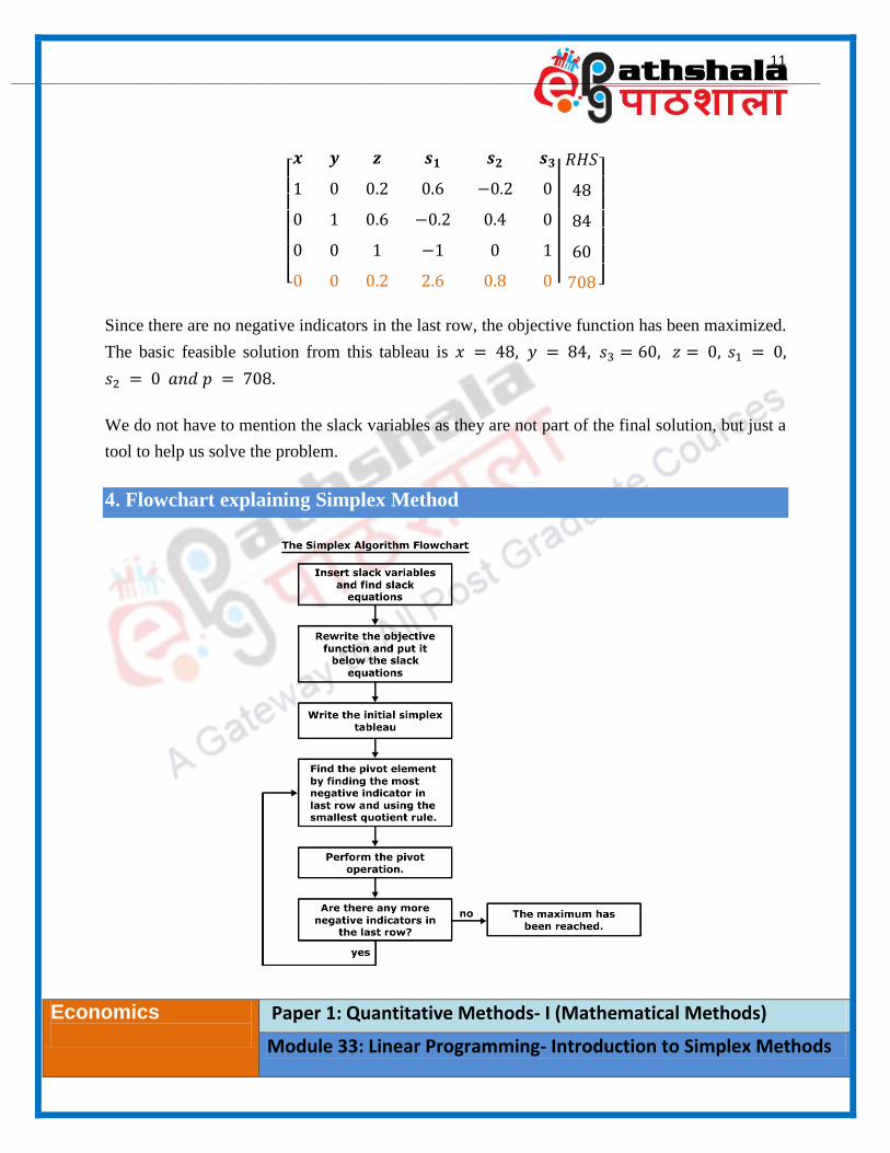
[ 𝒙 𝒚 𝒛 𝒔𝟏 𝒔𝟐 𝒔𝟑

1 0 0.2 0.6 −0.2 0

0 1 0.6 −0.2 0.4 0

0 0 1 −1 0 1

0 0 0.2 2.6 0.8 0

|

|

𝑅𝐻𝑆

48

84

60

708 ]

Since there are no negative indicators in the last row, the objective function has been maximized.

The basic feasible solution from this tableau is 𝑥 = 48, 𝑦 = 84, 𝑠3 = 60, 𝑧 = 0, 𝑠1 = 0,

𝑠2 = 0 𝑎𝑛𝑑 𝑝 = 708.

We do not have to mention the slack variables as they are not part of the final solution, but just a

tool to help us solve the problem.

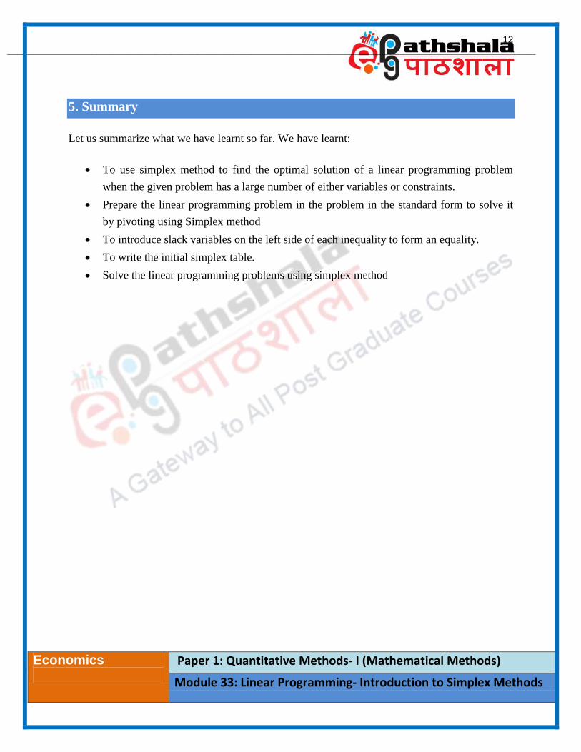
4. Flowchart explaining Simplex Method

____________________________________________________________________________________________________

Economics



12

5. Summary

Let us summarize what we have learnt so far. We have learnt:

To use simplex method to find the optimal solution of a linear programming problem

when the given problem has a large number of either variables or constraints.

Prepare the linear programming problem in the problem in the standard form to solve it

by pivoting using Simplex method

To introduce slack variables on the left side of each inequality to form an equality.

To write the initial simplex table.

Solve the linear programming problems using simplex method

Documents

Subject ECONOMICS Paper No and Title 1: Quantitative