Izmir University of Economics Econ 533: Quantitative

Izmir University of EconomicsEcon 533: Quantitative Methods and

Econometrics

One Variable Calculus

Izmir University of Economics Econ 533: Quantitative Methods and Econometrics

Introduction

I Finding the best way to do a speci�c task involves what iscalled an optimization problem.

I Studying an optimization problem requires mathematicalmethods of maximizing or minimizing a a function of a singlevariable.

I Useful economic insights can be gained from simple onevariable optimization.


Introduction

I Those points in the domain of a function where it reaches itslargest and smallest values are referred to as maximum andminimum points or extreme points. Thus, if f (x) has domainD, thenc ∈ D is a maximum point for f ⇔ f (x) ≤ f (c) for all x ∈ D

d ∈ D is a minimum point for f ⇔ f (x) ≥ f (d) for all x ∈ D

I If the value of f is strictly larger than any other point in D,then c is a strict maximum point. Similarly, d is a strictninimum point if f (x) > f (d) for all x ∈ D, x 6= d .

I Example 1: Find possible maximum and minimum points for

1. f (x) = 3− (x − 2)2

2. g(x) =√x − 5− 100, x ≥ 5


Necessary First Order Condition

Theorem

Suppose that a function f is di�erentiable in an interval I and that

c is an interior point of I . For x = c to be a maximum or a

minimum point of F in I , a necessary condition is that it is a critical

(stationary) point for f - i.e. that x = c satis�es the equation

f ′(x) = 0(�rst order condition)


First Derivative Test for Maximum/Minimum

Theorem

If f ′(x) ≥ 0 for x ≤ c and f ′(x) ≤ 0 for x ≥ c, then x = c is a

maximum point for f .

If f ′(x) ≤ 0 for x ≤ c and f ′(x) ≥ 0 for x ≥ c, then x = c is a

minimum point for f .

Example: Measured in miligrams per litre, the concentration of adrug in the bloodstream t hours after injection is given by theformula

c(t) =t

t2 + 4, t ≥ 0

Find the time of maximum concentration.


Convex and concave functions

f ′′(x) ≥ 0 on I ⇔ f ′ is increasing on I

f ′′(x) ≤ 0 on I ⇔ f ′ is decreasing on I

Assuming that f is continuous in the interval I and twicedi�erentiable in the interior of I :f is convex on I ⇔ f ′′(x) ≥ 0 for all x in I

f is concave on I ⇔ f ′′(x) ≤ 0 for all x in I

Maximum/Minimum for Concave/Convex Functions

Theorem

Suppose that a function f is concave (convex) in an interval I . If c

is a critical point of f in the interior of I , then c is a maximum

(minimum) point of f in I .

Example: Show that f (x) = ex−1 − 1 is convex and �nd itsminimum point.


Economic Examples 1

Example 1: Suppose Y (N) bushels of wheat are harvested per acreof land when N pounds of fertilizer per acre are used. If P is thedollar price per bushel of wheat and q is the dollar price per poundof fertilizer, the pro�ts in dollars per acre are

π(N) = PY (N)− qN, N ≥ 0

Suppose there exists N∗ such that π′(N) ≥ 0 for N ≤ N∗, whereasπ′(N) ≤ 0 for N ≥ N∗. Then N∗ maximizes pro�ts, andπ′(N∗) = 0. That is, PY ′(N∗)− q = 0, so

PY ′(N∗) = q

In a constructed example Y (N) =√N, P = 10, and q = 0.5. Find

the amount of fertilizer which maximizes pro�t in this case.


Example 2: The total cost of producing Q units of a commodity is

C (Q) = 2Q2 + 10Q + 32, Q > 0

Find the value of Q that minimizes the average cost.The total cost of producing Q units of a commodity is

C (Q) = aQ2 + bQ + c, Q > 0

where a, b, and c are positive constants. Show that average costfunction has a minimum at Q∗ =

√c/a.

Example 3: A monopolist is faced with the demand function P(Q)denoting the price when output is Q. The monopolist has aconstant average cost k per unit produced. Find the pro�t functionπ(Q), and the �rst order condition for maximum pro�t.


The Extreme Value Theorem

Theorem

If f is a continuous function over a closed bounded interval [a, b],then there exists a point d in [a, b] where f has a minimum, and a

point c in [a, b] where f has a maximum, so that

f (d) ≤ f (x) ≤ f (c) for all x in [a, b]


The recipe for �nding maximum amd minimum valuesProblem: Find the maximum and minimum values of adi�erentiable function f de�ned on a closed, bounded interval [a, b].Solution:

1. Find all critical points of f in (a, b) - that is �nd all points x in(a, b) that satisfy equation f ′(x) = 0.

2. Evaluate f at the end points a and b of the interval and at allstationary points.

3. The largest function value found in (2) is the maximum valueand the smallest function value is the minimum value of f in[a, b].

Example: Find the maximum and minimum values for

f (x) = 3x2 − 6x + 5, x ∈ [0, 3]


Further Economic Examples

Example: The total revenue of a single product �rm is R(Q)dollars, wheras C (Q) is the associated dollar cost. Assume Q̄ is themaximum quantity that can be produced and R and C aredi�erentiable functions of Q in the interval [0, Q̄]. The pro�tfunction is then di�erentiable, so continuous. Thus, π has amaximum value. In special cases, maximum might occur at Q = 0or at Q = Q̄. If not, it has an interior maximum where theproduction level Q∗ satis�es π′(Q∗) = 0, and so

R′(Q∗) = C

′(Q∗)

Production should be adjusted to a point where marginal revenue isequal to the marginal cost. The approximate extra revenue earnedby selling extra unit is o�set by the approximate extra cost ofproducing that unit.


Local Extreme Points

I Global optimization problems seek the largest or smallestvalues of a function at ALL points in the domain.

I Local optimization problems look at only the nearby points to�nd the the largest or smallest values of a function.

I The function f has a local maximum (minimum) at c, if thereexists an interval (α, β) about c such that f (x) ≤ (≥) f (c) forall x in (α, β) which are in the domain of f .

I At a local extreme point in the interior of the domain of a

di�erentiable function, the derivative must be zero.


Local Extreme Points

I In order to �nd possible local maxima and minima for afunction f de�ned in the interval I we search among thefollowing types of point:

i. Interior points in I where f ′(x) = 0ii. End points of Iiii. Interior points in I where f ′ does not exist

I How do we decide whether a point satisfying the necessaryconditions is a local max, local min, or neither?


The First Derivative Test

Theorem

Suppose c is a stationary point for y = f (x).

a. If f ′(x) ≥ 0 throughout some interval (a, c) to the left of c andf ′(x) ≤ 0 throughout some interval (c, b) to the right of c, thenx = c is a local maximum point for f .

b. If f ′(x) ≤ 0 throughout some interval (a, c) to the left of c andf ′(x) ≥ 0 throughout some interval (c, b) to the right of c, thenx = c is a local minimum point for f .

c. If f ′(x) > 0 both throughout some interval (a, c) to the left of cand throughout some interval (c, b) to the right of c, then x = c isnot a local extremum point for f . The same condition holds iff ′(x) < 0 on both sides of c.


The Second Derivative Test

Theorem

Let f be a twice di�erentiable function in an interval I , and let c be

an interior point of I . Then:

a. f ′(c) = 0 and f ′′(c) < 0 ⇒ x = c is a strict local maximum

point

b. f ′(c) = 0 and f ′′(c) > 0 ⇒ x = c is a strict local minimum

point

c. f ′(c) = 0 and f ′′(c) = 0 ⇒ ?


Examples

1. Classify the stationary points of f (x) = 1

9x3 - 1

6x2-2

3x + 1 and

f (x) = x2ex by using the �rst derivative test and secondderivative test.

2. Suppose that the �rm faces a sales tax of t dollars per unit.The �rm's pro�t from producing and selling Q units is then

π(Q) = R(Q)− C (Q)− tQ

In order to maximize pro�ts at some quantity Q∗ satisfying0 < Q∗ < Q̄, one must have π′(Q) = 0. Hence,

R ′(Q)− C ′(Q)− t = 0

Suppose R ′′(Q∗) < 0 and C ′′(Q∗) > 0. This equationimplicitly de�nes Q∗ as a di�erentiable function of t. Find anexpression for dQ∗/dt and discuss its sign.


Examples

1. Classify the stationary points of f (x) = 1

9x3 - 1

6x2-2

3x + 1 and

f (x) = x2ex by using the �rst derivative test and secondderivative test.

2. Suppose that the �rm faces a sales tax of t dollars per unit.The �rm's pro�t from producing and selling Q units is then

π(Q) = R(Q)− C (Q)− tQ

In order to maximize pro�ts at some quantity Q∗ satisfying0 < Q∗ < Q̄, one must have π′(Q) = 0. Hence,

R ′(Q)− C ′(Q)− t = 0

Suppose R ′′(Q∗) < 0 and C ′′(Q∗) > 0. This equationimplicitly de�nes Q∗ as a di�erentiable function of t. Find anexpression for dQ∗/dt and discuss its sign.


In�ection Points

I A twice di�erentiable function f (x) is concave (convex) inan interval I with f ′′(x) ≤ 0(≥) for all x in I .

I Points at which a function changes from being concave toconvex, or vice versa, are called in�ection points.

I For twice di�erentiable functions the de�nition is the following:The point c is called an in�ection point for the function f ifthere exists an interval (a, b) about c such that:

a. f ′′(x) ≥ 0 in (a, c) and f ′′(x) ≤ 0 in (c, b), orb. f ′′(x) ≤ 0 in (a, c) and f ′′(x) ≥ 0 in (c, b).


Test for In�ection Points

Theorem

Let f be a function with a continuous second derivative in an

interval I , and let c be an interior point of I .

a. If c is an in�ection point for f , then f ′′(c) = 0.

b. If f ′′(c) = 0 and f ′′ changes sign at c, then c is an in�ection

point for f .

Examples

1. Show that f (x) = x4 does not have an in�ection point atx = 0, even though f ′′(0) = 0.

2. Find possible in�ection points for f (x) = x6 − 10x4.


Production function

Suppose that x = f (v), v ≥ 0 is a production function. It isassumed that the function is S-shaped. That is the marginalproduct f ′(v) is increasing up to a certain production level v0, andthen decreasing. If f is twice di�erentiable, the f ′′(v) is ≥ 0 in[0, v0] and ≤ 0 in [v0,∞]. Hence, f is �rst convex and thenconcave, with v0 as an in�ection point. Note that at v0 a unitincrease in input gives the maximum increase in output.


Strictly Concave and Convex Functions

I A function is strictly concave (convex) if the line segmentjoining any two points on the graph is strictly below (above)the graph

I Obvious su�cient conditions for strict concavity/convexity arethe following:

I f ′′(x) < 0 for all x ∈ (a, b) ⇒ f (x) is strictly concave in (a, b)I f ′′(x) > 0 for all x ∈ (a, b) ⇒ f (x) is strictly convex in (a, b)

I The reverse implications are not correct. For instance,f (x) = x4 is strictly convex in the interval (−∞,∞), butf ′′(x) is not > 0 everywhere because f ′′(0) = 0.


Implicit Di�erentiation

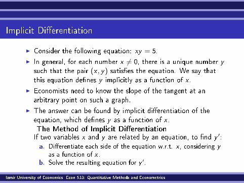
I Consider the following equation: xy = 5.

I In general, for each number x 6= 0, there is a unique number ysuch that the pair (x , y) satis�es the equation. We say thatthis equation de�nes y implicitly as a function of x .

I Economists need to know the slope of the tangent at anarbitrary point on such a graph.

I The answer can be found by implicit di�erentiation of theequation, which de�nes y as a function of x .The Method of Implicit Di�erentiationIf two variables x and y are related by an equation, to �nd y ′:a. Di�erentiate each side of the equation w.r.t. x , considering y

as a function of x .b. Solve the resulting equation for y ′.


Economic Examples

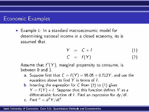
I Example 1: In a standard macroeconomic model fordetermining national income in a closed economy, its isassumed that

Y = C + I (1)

C = f (Y ) (2)

Assume that f ′(Y ), marginal propensity to consume, isbetween 0 and 1.a. Suppose �rst that C = f (Y ) = 95.05 + 0.712Y , and use the

equations above to �nd Y in terms of I .b. Inserting the expression for C from (2) to (1) gives

Y = f (Y ) + I . Suppose that this function de�nes Y as adi�erentiable function of I . Find an expression for dy/dI .

c. Find ′′ = d2Y /dI 2


Economic Examples

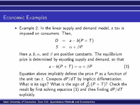
I Example 2: In the linear supply and demand model, a tax isimposed on consumers. Then,

D = a − b(P + T )

S = α + βP

Here a, b, α, and β are positive constants. The equilibriumprice is determined by equating supply and demand, so that

a − b(P + T ) = α + βP (3)

Equation above implicitly de�nes the price P as a function ofthe unit tax t. Compute dP/dT by implicit di�erentiation.What is its sign? What is the sign of d

dT(P + T )? Check the

result by �rst solving equation (3) and then �nding dP/dTexplicitly.


Elasticities

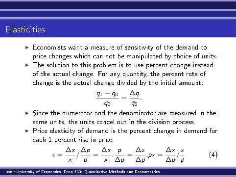
I Economists want a measure of sensitivity of the demand toprice changes which can not be manipulated by choice of units.

I The solution to this problem is to use percent change insteadof the actual change. For any quantity, the percent rate ofchange is the actual change divided by the initial amount:

q1 − q0q0

=∆q

q0.

I Since the numerator and the denominator are measured in thesame units, the units cancel out in the division process.

I Price elasticity of demand is the percent change in demand foreach 1 percent rise in price.

ε =∆x

x/

∆p

p=

∆x

x.p

∆p=

∆x

∆p.px =

∆x

∆p/x

p(4)


Elasticities

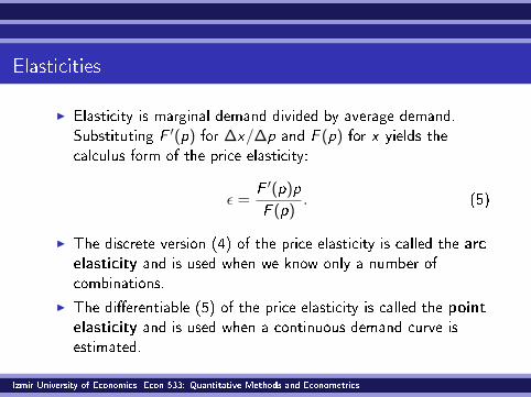
I Elasticity is marginal demand divided by average demand.Substituting F ′(p) for ∆x/∆p and F (p) for x yields thecalculus form of the price elasticity:

ε =F ′(p)p

F (p). (5)

I The discrete version (4) of the price elasticity is called the arcelasticity and is used when we know only a number ofcombinations.

I The di�erentiable (5) of the price elasticity is called the pointelasticity and is used when a continuous demand curve isestimated.


Elasticities

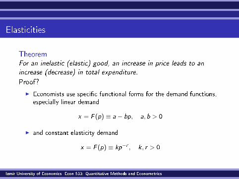
Theorem

For an inelastic (elastic) good, an increase in price leads to an

increase (decrease) in total expenditure.

Proof?

I Economists use speci�c functional forms for the demand functions,especially linear demand

x = F (p) ≡ a− bp, a, b > 0

I and constant elasticity demand

x = F (p) ≡ kp−r , k, r > 0


Elasticities

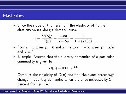
I Since the slope of F di�ers from the elasticity of F , theelasticity varies along a demand curve:

ε =F ′(p)p

F (p)=−bpa − bp

=1

1− (a/bp)

I from ε = 0 when p = 0 and x = a to ε = −∞ when p = a/band x = 0.

I Example: Assume that the quantity demanded of a particularcommodity is given by

D(p) = 8000p−1.5

Compute the elasticity of D(p) and �nd the exact percentagechange in quantity demanded when the price increases by 1percent from p = 4.


Intermediate Value Theorem: Newton Method

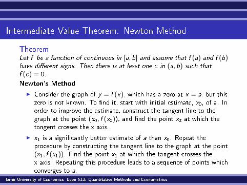
Theorem

Let f be a function of continuous in [a, b] and assume that f (a) and f (b)have di�erent signs. Then there is at least one c in (a, b) such thatf (c) = 0.

Newton's Method

I Consider the graph of y = f (x), which has a zero at x = a, but thiszero is not known. To �nd it, start with initial estimate, x0, of a. Inorder to improve the estimate, construct the tangent line to thegraph at the point (x0, f (x0)), and �nd the point x2 at which thetangent crosses the x-axis.

I x1 is a signi�cantly better estimate of a than x0. Repeat theprocedure by constructing the tangent line to the graph at the point(x1, f (x1)). Find the point x1 at which the tangent crosses thex-axis. Repeating this procedure leads to a sequence of points whichconverges to a.


Newton's Method

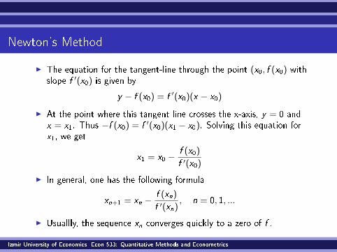
I The equation for the tangent-line through the point (x0, f (x0) withslope f ′(x0) is given by

y − f (x0) = f ′(x0)(x − x0)

I At the point where this tangent line crosses the x-axis, y = 0 andx = x1. Thus −f (x0) = f ′(x0)(x1 − x0). Solving this equation forx1, we get

x1 = x0 −f (x0)

f ′(x0)

I In general, one has the following formula

xn+1 = xn −f (xn)

f ′(xn), n = 0, 1, ...

I Usuallly, the sequence xn converges quickly to a zero of f .


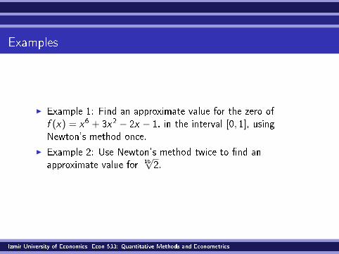
Examples

I Example 1: Find an approximate value for the zero off (x) = x6 + 3x2 − 2x − 1, in the interval [0, 1], usingNewton's method once.

I Example 2: Use Newton's method twice to �nd anapproximate value for 15

√2.


Documents

Izmir University of Economics Econ 533: Quantitative