Embed Size (px)
Citation preview

Quantitative Economics for the Evaluation of the
European Policy
Dipartimento di Economia e Management
Irene Brunetti Davide Fiaschi Angela Parenti1
04/10/2016
[email protected], [email protected], and [email protected] Quantitative Economics 04/10/2016 1 / 21
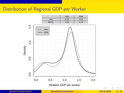
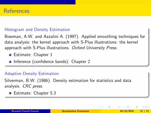
Distribution of Regional GDP per Worker
0.0 0.5 1.0 1.5 2.0
0.0
0.5
1.0
1.5
Relative GDP per worker
Den
sity
19912008
1991 2008
Gini 0.25 0.23
BIPOL 0.83 0.78
Brunetti-Fiaschi-Parenti Quantitative Economics 04/10/2016 2 / 21
Estimate of The Density Function
Let be x a continuous random variable and f its probability densityfunction (pdf).The pdf characterizes the distribution of the random variable x since ittells “how x is distributed”.Moreover, from pdf it is possible to calculate the mean and the variance(it they exists) of x and the probability that x takes on values in a giveninterval.
Brunetti-Fiaschi-Parenti Quantitative Economics 04/10/2016 3 / 21
Histogram
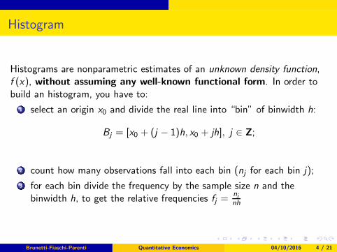
Histograms are nonparametric estimates of an unknown density function,f (x), without assuming any well-known functional form. In order tobuild an histogram, you have to:
1 select an origin x0 and divide the real line into “bin” of binwidth h:
Bj = [x0 + (j − 1)h, x0 + jh], j ∈ Z;
Brunetti-Fiaschi-Parenti Quantitative Economics 04/10/2016 4 / 21
Histogram
Histograms are nonparametric estimates of an unknown density function,f (x), without assuming any well-known functional form. In order tobuild an histogram, you have to:
1 select an origin x0 and divide the real line into “bin” of binwidth h:
Bj = [x0 + (j − 1)h, x0 + jh], j ∈ Z;
2 count how many observations fall into each bin (nj for each bin j);
3 for each bin divide the frequency by the sample size n and thebinwidth h, to get the relative frequencies fj =
njnh
Brunetti-Fiaschi-Parenti Quantitative Economics 04/10/2016 4 / 21
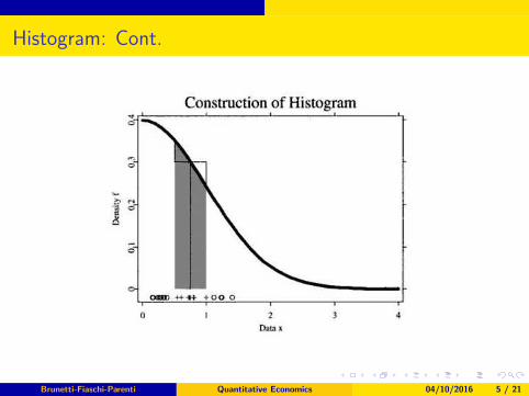
Histogram: Cont.
Brunetti-Fiaschi-Parenti Quantitative Economics 04/10/2016 5 / 21
Histogram: Cont.
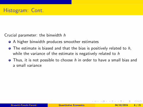
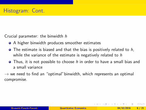
Crucial parameter: the binwidth h
A higher binwidth produces smoother estimates
Brunetti-Fiaschi-Parenti Quantitative Economics 04/10/2016 6 / 21
Histogram: Cont.
Crucial parameter: the binwidth h
A higher binwidth produces smoother estimates
The estimate is biased and that the bias is positively related to h,while the variance of the estimate is negatively related to h
Brunetti-Fiaschi-Parenti Quantitative Economics 04/10/2016 6 / 21
Histogram: Cont.
Crucial parameter: the binwidth h
A higher binwidth produces smoother estimates
The estimate is biased and that the bias is positively related to h,while the variance of the estimate is negatively related to h
Thus, it is not possible to choose h in order to have a small bias anda small variance
→ we need to find an “optimal”binwidth, which represents an optimalcompromise.
Brunetti-Fiaschi-Parenti Quantitative Economics 04/10/2016 6 / 21

Histogram: Cont.
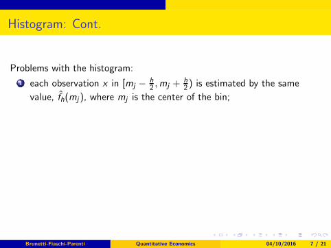
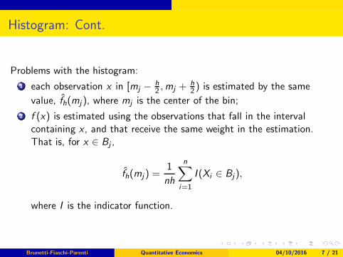
Problems with the histogram:
Brunetti-Fiaschi-Parenti Quantitative Economics 04/10/2016 7 / 21
Histogram: Cont.
Problems with the histogram:
1 each observation x in [mj −h2,mj +
h2) is estimated by the same
value, f̂h(mj ), where mj is the center of the bin;
Brunetti-Fiaschi-Parenti Quantitative Economics 04/10/2016 7 / 21
Histogram: Cont.
Problems with the histogram:
1 each observation x in [mj −h2,mj +
h2) is estimated by the same
value, f̂h(mj ), where mj is the center of the bin;
2 f (x) is estimated using the observations that fall in the intervalcontaining x , and that receive the same weight in the estimation.That is, for x ∈ Bj ,
f̂h(mj ) =1
nh
n∑
i=1
I (Xi ∈ Bj),
where I is the indicator function.
Brunetti-Fiaschi-Parenti Quantitative Economics 04/10/2016 7 / 21
Nonparametric density estimation
Density estimation is a generalization of the histogram.
Brunetti-Fiaschi-Parenti Quantitative Economics 04/10/2016 8 / 21
Nonparametric density estimation
Density estimation is a generalization of the histogram.
It is based on Kernel functions: estimate f (x) using theobservations that fall into an interval around x , which (typically)receive decreasing weight the further they are from x .
Brunetti-Fiaschi-Parenti Quantitative Economics 04/10/2016 8 / 21
Kernel functions
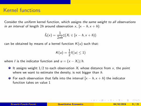
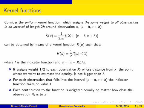
Consider the uniform kernel function, which assigns the same weight to all observations
in an interval of length 2h around observation x , [x − h, x + h):
f̂h(x) =1
2nh♯{Xi ∈ [x − h, x + h)}
can be obtained by means of a kernel function K(u) such that:
K(u) =1
2I (|u| ≤ 1)
where I is the indicator function and u = (x − Xi )/h.
Brunetti-Fiaschi-Parenti Quantitative Economics 04/10/2016 9 / 21
Kernel functions
Consider the uniform kernel function, which assigns the same weight to all observations
in an interval of length 2h around observation x , [x − h, x + h):
f̂h(x) =1
2nh♯{Xi ∈ [x − h, x + h)}
can be obtained by means of a kernel function K(u) such that:
K(u) =1
2I (|u| ≤ 1)
where I is the indicator function and u = (x − Xi )/h.
It assigns weight 1/2 to each observation Xi whose distance from x , the pointwhere we want to estimate the density, is not bigger than h.
For each observation that falls into the interval [x − h, x + h) the indicatorfunction takes on value 1
Each contribution to the function is weighted equally no matter how close theobservation Xi is to x
Brunetti-Fiaschi-Parenti Quantitative Economics 04/10/2016 9 / 21
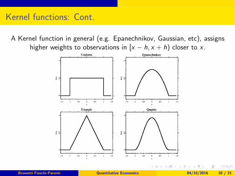
Kernel functions: Cont.
A Kernel function in general (e.g. Epanechnikov, Gaussian, etc), assignshigher weights to observations in [x − h, x + h) closer to x .
Brunetti-Fiaschi-Parenti Quantitative Economics 04/10/2016 10 / 21
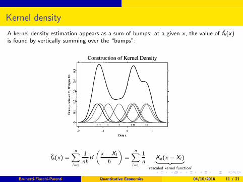
Kernel density
A kernel density estimation appears as a sum of bumps: at a given x , the value of f̂h(x)is found by vertically summing over the “bumps”:
f̂h(x) =
n∑
i=1
1
nhK
(x − Xi
h
)
=
n∑
i=1
1
nKh(x − Xi )︸ ︷︷ ︸
“rescaled kernel function”
Brunetti-Fiaschi-Parenti Quantitative Economics 04/10/2016 11 / 21
Properties of Kernel density estimator
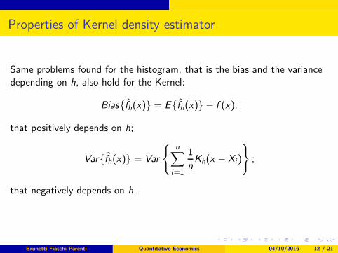
Same problems found for the histogram, that is the bias and the variancedepending on h, also hold for the Kernel:
Bias{f̂h(x)} = E{f̂h(x)} − f (x);
that positively depends on h;
Var{f̂h(x)} = Var
{
n∑
i=1
1
nKh(x − Xi)
}
;
that negatively depends on h.
Brunetti-Fiaschi-Parenti Quantitative Economics 04/10/2016 12 / 21
Properties of Kernel density estimator
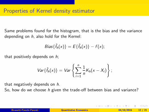
Same problems found for the histogram, that is the bias and the variancedepending on h, also hold for the Kernel:
Bias{f̂h(x)} = E{f̂h(x)} − f (x);
that positively depends on h;
Var{f̂h(x)} = Var
{
n∑
i=1
1
nKh(x − Xi)
}
;
that negatively depends on h.So, how do we choose h given the trade-off between bias and variance?
Brunetti-Fiaschi-Parenti Quantitative Economics 04/10/2016 12 / 21
Choosing the bandwidth h
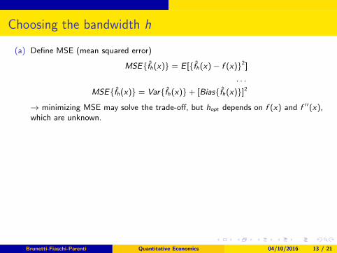
(a) Define MSE (mean squared error)
MSE{f̂h(x)} = E [{f̂h(x)− f (x)}2]
. . .
MSE{f̂h(x)} = Var{f̂h(x)}+ [Bias{f̂h(x)}]2
→ minimizing MSE may solve the trade-off, but hopt depends on f (x) and f ′′(x),which are unknown.
Brunetti-Fiaschi-Parenti Quantitative Economics 04/10/2016 13 / 21
Choosing the bandwidth h
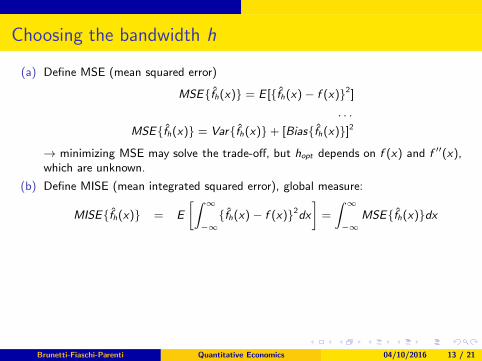
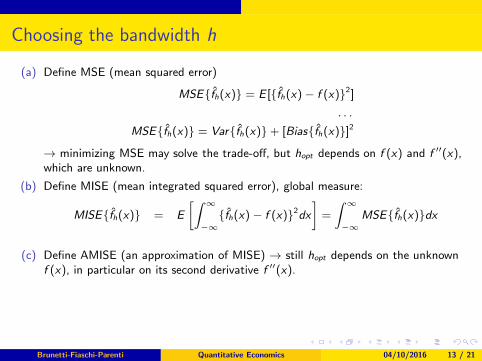
(a) Define MSE (mean squared error)
MSE{f̂h(x)} = E [{f̂h(x)− f (x)}2]
. . .
MSE{f̂h(x)} = Var{f̂h(x)}+ [Bias{f̂h(x)}]2
→ minimizing MSE may solve the trade-off, but hopt depends on f (x) and f ′′(x),which are unknown.
(b) Define MISE (mean integrated squared error), global measure:
MISE{f̂h(x)} = E
[∫∞
−∞
{f̂h(x) − f (x)}2dx
]
=
∫∞
−∞
MSE{f̂h(x)}dx
Brunetti-Fiaschi-Parenti Quantitative Economics 04/10/2016 13 / 21
Choosing the bandwidth h
(a) Define MSE (mean squared error)
MSE{f̂h(x)} = E [{f̂h(x)− f (x)}2]
. . .
MSE{f̂h(x)} = Var{f̂h(x)}+ [Bias{f̂h(x)}]2
→ minimizing MSE may solve the trade-off, but hopt depends on f (x) and f ′′(x),which are unknown.
(b) Define MISE (mean integrated squared error), global measure:
MISE{f̂h(x)} = E
[∫∞
−∞
{f̂h(x) − f (x)}2dx
]
=
∫∞
−∞
MSE{f̂h(x)}dx
(c) Define AMISE (an approximation of MISE) → still hopt depends on the unknownf (x), in particular on its second derivative f ′′(x).
Brunetti-Fiaschi-Parenti Quantitative Economics 04/10/2016 13 / 21
Choosing the bandwidth h
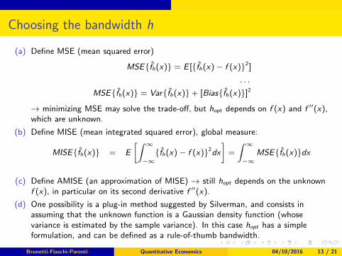
(a) Define MSE (mean squared error)
MSE{f̂h(x)} = E [{f̂h(x)− f (x)}2]
. . .
MSE{f̂h(x)} = Var{f̂h(x)}+ [Bias{f̂h(x)}]2
→ minimizing MSE may solve the trade-off, but hopt depends on f (x) and f ′′(x),which are unknown.
(b) Define MISE (mean integrated squared error), global measure:
MISE{f̂h(x)} = E
[∫∞
−∞
{f̂h(x) − f (x)}2dx
]
=
∫∞
−∞
MSE{f̂h(x)}dx
(c) Define AMISE (an approximation of MISE) → still hopt depends on the unknownf (x), in particular on its second derivative f ′′(x).
(d) One possibility is a plug-in method suggested by Silverman, and consists inassuming that the unknown function is a Gaussian density function (whosevariance is estimated by the sample variance). In this case hopt has a simpleformulation, and can be defined as a rule-of-thumb bandwidth.
Brunetti-Fiaschi-Parenti Quantitative Economics 04/10/2016 13 / 21
Adaptive Kernel
Up to know we have seen the possibility of giving higher weights tothe observations whose distance from x , the point where we want toestimate the density, is not bigger than h → assuming only one h!
Brunetti-Fiaschi-Parenti Quantitative Economics 04/10/2016 14 / 21
Adaptive Kernel
Up to know we have seen the possibility of giving higher weights tothe observations whose distance from x , the point where we want toestimate the density, is not bigger than h → assuming only one h!
But we can get a better estimate by allowing the window width of thekernels to vary from one point to another.
In particular, a natural way to deal with long-tailed densities is to usea broader kerne I in regions of low density.
Thus an observation in the tail would have its mass smudged out overa wider range than one in the main part of the distribution.
Brunetti-Fiaschi-Parenti Quantitative Economics 04/10/2016 14 / 21
Adaptive Kernel: Cont.
A practical problem is deciding in the first place whether or not anobservation is in a region of low density
Brunetti-Fiaschi-Parenti Quantitative Economics 04/10/2016 15 / 21
Adaptive Kernel: Cont.
A practical problem is deciding in the first place whether or not anobservation is in a region of low density
The adaptive kernel approach copes with this problem by means of atwo-stage procedure:
Brunetti-Fiaschi-Parenti Quantitative Economics 04/10/2016 15 / 21
Adaptive Kernel: Cont.
A practical problem is deciding in the first place whether or not anobservation is in a region of low density
The adaptive kernel approach copes with this problem by means of atwo-stage procedure:
1 get an initial estimate to have a rough idea of the density
Brunetti-Fiaschi-Parenti Quantitative Economics 04/10/2016 15 / 21
Adaptive Kernel: Cont.
A practical problem is deciding in the first place whether or not anobservation is in a region of low density
The adaptive kernel approach copes with this problem by means of atwo-stage procedure:
1 get an initial estimate to have a rough idea of the density2 use the former density to get a pattern of bandwidths corresponding to
various observations to be used in a second estimate
Brunetti-Fiaschi-Parenti Quantitative Economics 04/10/2016 15 / 21
Adaptive Kernel: Cont.
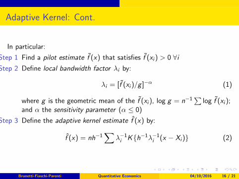
In particular:
Step 1 Find a pilot estimate f̃ (x) that satisfies f̃ (xi ) > 0 ∀i
Brunetti-Fiaschi-Parenti Quantitative Economics 04/10/2016 16 / 21
Adaptive Kernel: Cont.
In particular:
Step 1 Find a pilot estimate f̃ (x) that satisfies f̃ (xi ) > 0 ∀i
Step 2 Define local bandwidth factor λi by:
λi = [f̃ (xi )/g ]−α (1)
where g is the geometric mean of the f̃ (xi ), log g = n−1∑
log f̃ (xi );and α the sensitivity parameter (α ≤ 0)
Step 3 Define the adaptive kernel estimate f̂ (x) by:
f̂ (x) = nh−1∑
λ−1
i K{h−1λ−1
i (x − Xi)} (2)
Brunetti-Fiaschi-Parenti Quantitative Economics 04/10/2016 16 / 21
Bootstrap
The bootstrap technique allows estimation of the populationdistribution by using the information based on a number of resamplesfrom the sample.
Brunetti-Fiaschi-Parenti Quantitative Economics 04/10/2016 17 / 21
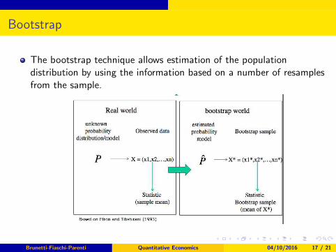
Bootstrap
The bootstrap technique allows estimation of the populationdistribution by using the information based on a number of resamplesfrom the sample.
Brunetti-Fiaschi-Parenti Quantitative Economics 04/10/2016 17 / 21

Bootstrap: Cont.
Use the information of a number of resamples from the sample toestimate the population distribution
Brunetti-Fiaschi-Parenti Quantitative Economics 04/10/2016 18 / 21
Bootstrap: Cont.
Use the information of a number of resamples from the sample toestimate the population distribution
Procedure:Given a sample of size n:
Brunetti-Fiaschi-Parenti Quantitative Economics 04/10/2016 18 / 21

Bootstrap: Cont.
Use the information of a number of resamples from the sample toestimate the population distribution
Procedure:Given a sample of size n:
Treat the sample as population
Brunetti-Fiaschi-Parenti Quantitative Economics 04/10/2016 18 / 21
Bootstrap: Cont.
Use the information of a number of resamples from the sample toestimate the population distribution
Procedure:Given a sample of size n:
Treat the sample as populationDraw B samples of size n with replacement from your sample (thebootstrap samples)
Brunetti-Fiaschi-Parenti Quantitative Economics 04/10/2016 18 / 21
Bootstrap: Cont.
Use the information of a number of resamples from the sample toestimate the population distribution
Procedure:Given a sample of size n:
Treat the sample as populationDraw B samples of size n with replacement from your sample (thebootstrap samples)Compute for each bootstrap sample the statistic of interest
Brunetti-Fiaschi-Parenti Quantitative Economics 04/10/2016 18 / 21
Bootstrap: Cont.
Use the information of a number of resamples from the sample toestimate the population distribution
Procedure:Given a sample of size n:
Treat the sample as populationDraw B samples of size n with replacement from your sample (thebootstrap samples)Compute for each bootstrap sample the statistic of interestEstimate the sample distribution of the statistic by the bootstrapsample distribution
Brunetti-Fiaschi-Parenti Quantitative Economics 04/10/2016 18 / 21
Bootstrap: Cont.
Basic idea: If the sample is a good approximation of the population,bootstrapping will provide a good approximation of the sampledistribution.
Brunetti-Fiaschi-Parenti Quantitative Economics 04/10/2016 19 / 21
Bootstrap: Cont.
Basic idea: If the sample is a good approximation of the population,bootstrapping will provide a good approximation of the sampledistribution.
Justification:
Brunetti-Fiaschi-Parenti Quantitative Economics 04/10/2016 19 / 21
Bootstrap: Cont.
Basic idea: If the sample is a good approximation of the population,bootstrapping will provide a good approximation of the sampledistribution.
Justification:1 If the sample is representative for the population, the sample
distribution (empirical distribution) approaches the population(theoretical) distribution if n increases;
2 If the number of resamples (B) from the original sample increases, thebootstrap distribution approaches the sample distribution.
Brunetti-Fiaschi-Parenti Quantitative Economics 04/10/2016 19 / 21
Bootstrap Procedure for Confidence Bands
Given a sample of observations X = {X1, ...,Xm} where each Xi is avector of dimension n the bootstrap algorithm is the following.
Brunetti-Fiaschi-Parenti Quantitative Economics 04/10/2016 20 / 21
Bootstrap Procedure for Confidence Bands
Given a sample of observations X = {X1, ...,Xm} where each Xi is avector of dimension n the bootstrap algorithm is the following.
1 Estimate from sample x the density f̂ .
Brunetti-Fiaschi-Parenti Quantitative Economics 04/10/2016 20 / 21
Bootstrap Procedure for Confidence Bands
Given a sample of observations X = {X1, ...,Xm} where each Xi is avector of dimension n the bootstrap algorithm is the following.
1 Estimate from sample x the density f̂ .
2 Select B independent bootstrap samples {X ∗1, ...,X ∗B}, eachconsisting of n data values drawn with replacement from x .
3 Estimate the density f̂ ∗b corresponding to each bootstrap sampleb = 1, ...,B .
The distribution of f̂ ∗ about f̂ can therefore be used to mimic thedistribution of f̂ about f , that is it can be used to calculate the confidenceintervals for estimates.
Brunetti-Fiaschi-Parenti Quantitative Economics 04/10/2016 20 / 21
References
Histogram and Density Estimation
Bowman, A.W. and Azzalini A. (1997). Applied smoothing techniques fordata analysis: the kernel approach with S-Plus illustrations: the kernelapproach with S-Plus illustrations. Oxford University Press.
Estimate: Chapter 1
Inference (confidence bands): Chapter 2
Adaptive Density Estimation
Silverman, B.W. (1986). Density estimation for statistics and dataanalysis. CRC press.
Estimate: Chapter 5.3
Brunetti-Fiaschi-Parenti Quantitative Economics 04/10/2016 21 / 21


![JKE 316E – Quantitative Economics [Ekonomi Kuantitatif]](https://img.pdfslide.us/doc/110x75/627325941b5cc94fcb3feaff/jke-316e-quantitative-economics-ekonomi-kuantitatif.jpg)