ECONOMICS Paper 1: Quantitative Methods- I (Mathematical

____________________________________________________________________________________________________

ECONOMICS

Paper 1: Quantitative Methods- I (Mathematical Methods)

Module 37: Linear Programming - Two Phase Simplex Method and Dual Simplex

1

Subject ECONOMICS

Paper No and Title 1: Quantitative Methods- I (Mathematical Methods)

Module No and Title 37: Linear Programming - Two Phase Simplex Method and

Dual Simplex

Module Tag ECO_P1_M37

____________________________________________________________________________________________________

ECONOMICS



2

TABLE OF CONTENTS

1. Learning Outcomes

2. Introduction

3. Two-Phase Method

3.1. Phase I

3.2. Phase II

4. Dual Simplex Method

4.1. Modification of Constraint

4.2. Checking Modified Problem

4.3. Selection of exiting variable

4.4. Selection of entering variable

4.5. Pivotal Operation

4.6. Check for optimality

5. Summary

____________________________________________________________________________________________________

ECONOMICS



3

1. Learning Outcomes

After studying this module, you shall be able to:

Understand the Two-Phase Simplex Method

Learn Dual Simplex Method

Explore the difference between Dual Simplex and Simplex Method

2. Introduction

The simplex algorithm assumes that the initial point is feasible in the primal problem. If b is greater

than or equal to zero, then the origin is feasible. If the origin is not feasible, then it is necessary to

determine some other initial point that is feasible. It is possible to introduce an auxiliary primal

problem specifically designed to help in this task. The process of eliminating artificial variables is

performed in Phase-I of the solution and Phase-II is used to get an optimal solution. Since the

solution of LPP is computed in two phases, it is called as Two-Phase Simplex Method. There is

typically a need for elementary row operations to bring the tableau into the form required by the

simplex algorithm.

Computationally, dual simplex method is same as simplex method. However, their approaches are

different from each other. Simplex method initiates with a non-optimal but feasible solution

whereas dual simplex method initiates with a solution that is optimal but infeasible. Simplex

method is responsible for maintaining the feasibility while successive iterations are taking place

whereas on the other hand dual simplex method is responsible for maintaining the optimality.

____________________________________________________________________________________________________

ECONOMICS



4

The dual simplex algorithm is most sought after solution method for LPP. Adding newer

constraints to a LPP problem, customarily leads to the breakup of primal feasibility but not dual

feasibility, the dual simplex can be used for frequent re-optimization, barring the requirement of

searching solutions of new primal basic feasible. This is of the most use in integer programming,

where the use of cutting plane techniques require the introduction of newer constraints at various

stages of the branch-and-bound/cut/price algorithms.

This method helps in the provision of much simplistic ways to the two- phase method for the cases

where there is unfeasible starting solution. Dual-simplex method can be used where costs which

are reduced are positive values unlike the two phase method which can always be used.

3. Two-Phase Method

We consider the method of two-stage simplex with the following example.

Minimize x1 + 2x2

subject to x1 + x2 ≥ 4, x1 − x2 ≥ 1, −x1 + 2x2 ≥ −1

over x1 ≥ 0, x2 ≥ 0

which, adding slack variables, is equivalent to this first problem

Minimize x1 + 2x2

subject to x1 + x2 −z1 = 4,

x1 − x2 − z2 = 1,

−x1 +2x2 −z3 = −1,

over x1 ≥ 0, x2 ≥ 0, z1 ≥ 0, z2 ≥ 0, z3 ≥ 0.

____________________________________________________________________________________________________

ECONOMICS



5

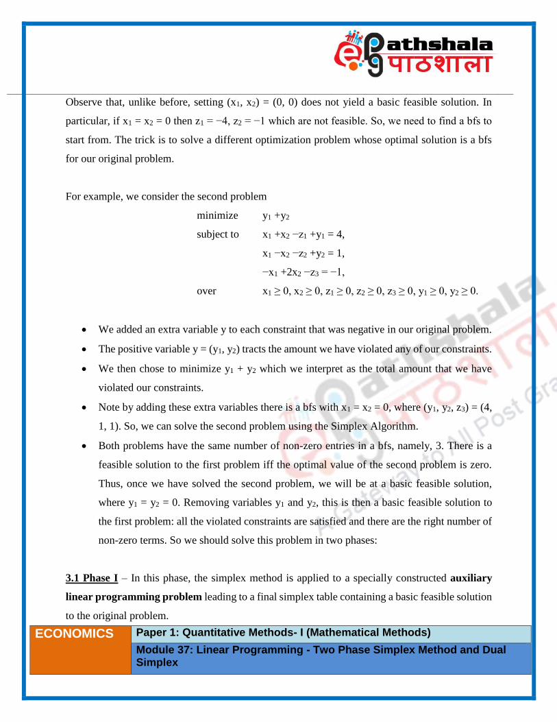
Observe that, unlike before, setting (x1, x2) = (0, 0) does not yield a basic feasible solution. In

particular, if x1 = x2 = 0 then z1 = −4, z2 = −1 which are not feasible. So, we need to find a bfs to

start from. The trick is to solve a different optimization problem whose optimal solution is a bfs

for our original problem.

For example, we consider the second problem

minimize y1 +y2

subject to x1 +x2 −z1 +y1 = 4,

x1 −x2 −z2 +y2 = 1,

−x1 +2x2 −z3 = −1,

over x1 ≥ 0, x2 ≥ 0, z1 ≥ 0, z2 ≥ 0, z3 ≥ 0, y1 ≥ 0, y2 ≥ 0.

We added an extra variable y to each constraint that was negative in our original problem.

The positive variable y = (y1, y2) tracts the amount we have violated any of our constraints.

We then chose to minimize y1 + y2 which we interpret as the total amount that we have

violated our constraints.

Note by adding these extra variables there is a bfs with x1 = x2 = 0, where (y1, y2, z3) = (4,

1, 1). So, we can solve the second problem using the Simplex Algorithm.

Both problems have the same number of non-zero entries in a bfs, namely, 3. There is a

feasible solution to the first problem iff the optimal value of the second problem is zero.

Thus, once we have solved the second problem, we will be at a basic feasible solution,

where y1 = y2 = 0. Removing variables y1 and y2, this is then a basic feasible solution to

the first problem: all the violated constraints are satisfied and there are the right number of

non-zero terms. So we should solve this problem in two phases:

3.1 Phase I – In this phase, the simplex method is applied to a specially constructed auxiliary

linear programming problem leading to a final simplex table containing a basic feasible solution

to the original problem.

____________________________________________________________________________________________________

ECONOMICS



6

Step 1 – Assign a cost -1 to each artificial variable and a cost 0 to all other variables in the

objective function.

Step 2 – Construct the Auxiliary LPP in which the new objective function Z* is to be

maximized subject to the given set of constraints.

Step 3 – Solve the auxiliary problem by simplex method until either of the following three

possibilities do arise

i. Max Z* < 0 and at least one artificial vector appear in the optimum basis at a

positive level (Δj ≥ 0). In this case, given problem does not possess any feasible

solution.

ii. Max Z* = 0 and at least one artificial vector appears in the optimum basis at a zero

level. In this case proceed to phase-II.

iii. Max Z* = 0 and no one artificial vector appears in the optimum basis. In this case

also proceed to phase-II.

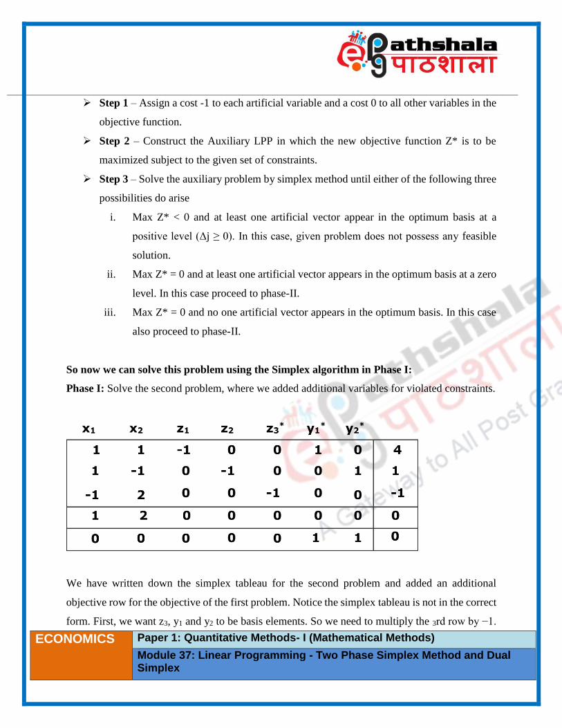
So now we can solve this problem using the Simplex algorithm in Phase I:

Phase I: Solve the second problem, where we added additional variables for violated constraints.

We have written down the simplex tableau for the second problem and added an additional

objective row for the objective of the first problem. Notice the simplex tableau is not in the correct

form. First, we want z3, y1 and y2 to be basis elements. So we need to multiply the 3rd row by −1.

____________________________________________________________________________________________________

ECONOMICS



7

Second, the Phase I objective row contains non-zero entries above basic feasible variables y1, y2.

So we need to subtract the first and second rows of the simplex tableau from the bottom objective

row.

We now proceed to optimize this tableau whilst treating the additional objective row as though it

was just an additional constraint.

____________________________________________________________________________________________________

ECONOMICS



8

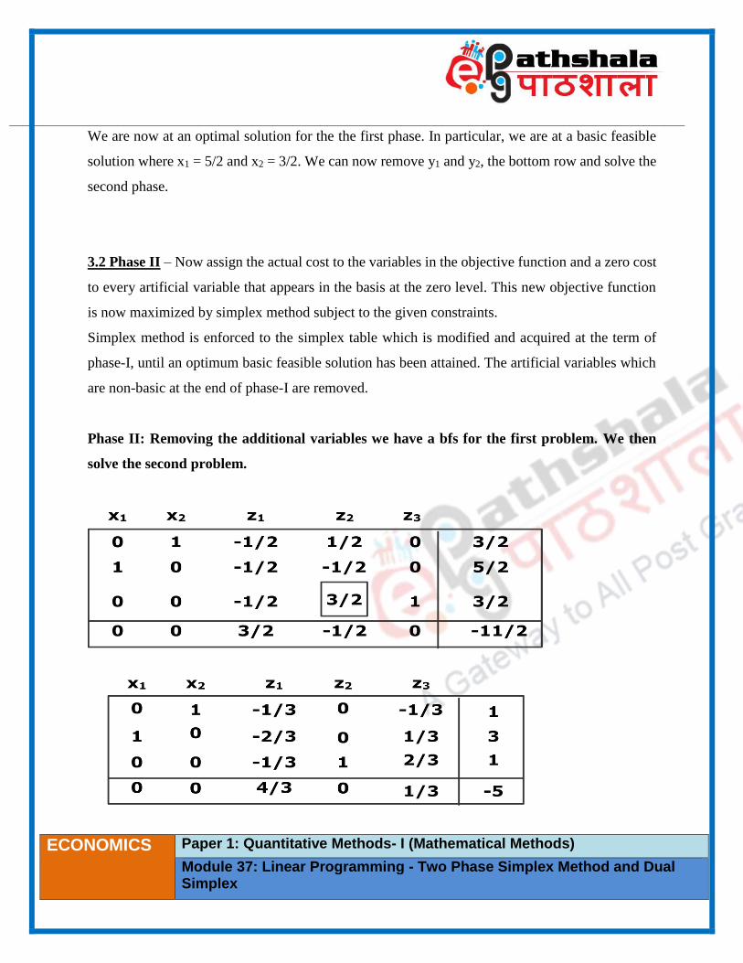
We are now at an optimal solution for the the first phase. In particular, we are at a basic feasible

solution where x1 = 5/2 and x2 = 3/2. We can now remove y1 and y2, the bottom row and solve the

second phase.

3.2 Phase II – Now assign the actual cost to the variables in the objective function and a zero cost

to every artificial variable that appears in the basis at the zero level. This new objective function

is now maximized by simplex method subject to the given constraints.

Simplex method is enforced to the simplex table which is modified and acquired at the term of

phase-I, until an optimum basic feasible solution has been attained. The artificial variables which

are non-basic at the end of phase-I are removed.

Phase II: Removing the additional variables we have a bfs for the first problem. We then

solve the second problem.

____________________________________________________________________________________________________

ECONOMICS



9

So we have now solved our original optimization problem. The optimal solution is x1 = 3, x2 = 1

with optimal value 5.

4. Dual Simplex Method

In the simplex method, row 0 elements would be negative for some till the final iteration when

conditions optimality are satisfied. In the case wherein all row 0 elements are nonnegative, there

is dual feasibility of associated basis. As matter of fact if row 0’s some elements are negative,

dual infeasible basis is achieved.

As explained, the primal simplex method is linked with primal feasible, however dual infeasible

bases. The basis is both primal as well as dual feasible at the final optimal solution. Primal

feasibility & drive toward dual feasibility is maintained all through the process.

Here, a primal approach variable, familiar as the dual simplex method, is recognized working in

the reverse fashion. Each basis inspected is primal infeasible (some negative values on the RHS)

& dual feasible (all elements in row 0 are nonnegative) till the final iteration. The solution would

be both primal as well as dual feasible at the final optimal iteraton. All through the process, dual

feasibility & drive toward primal feasibility is maintained. For a given question, both primal as

well as dual simplex algorithms will conclude at the same solution, nonetheless they will reach

from different directions.

Questions for which availability of an initial dual feasible solution is there, dual simplex algorithm

are most apt for such kind of problems.

Specifically it is fruitful to re-optimize a problem post the addition of constraint or post

modification of some parameters so as feasibility of previously optimal basis is no longer there.

____________________________________________________________________________________________________

ECONOMICS



10

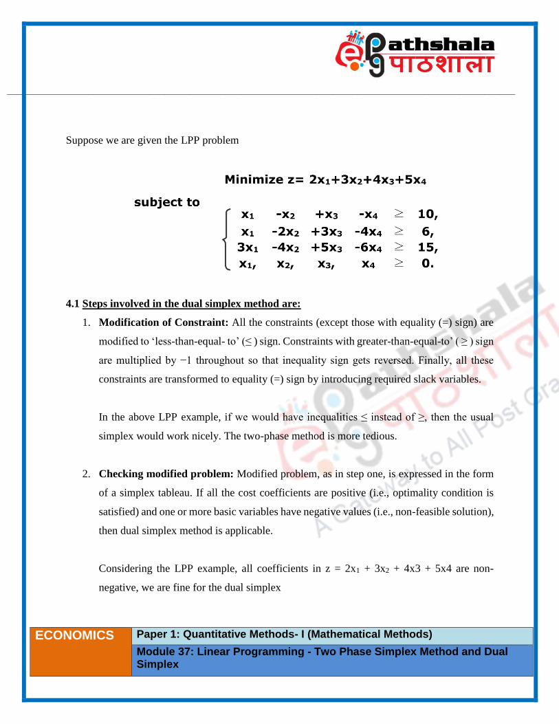
Suppose we are given the LPP problem

4.1 Steps involved in the dual simplex method are:

1. Modification of Constraint: All the constraints (except those with equality (=) sign) are

modified to ‘less-than-equal- to’ (≤ ) sign. Constraints with greater-than-equal-to’ ( ≥ ) sign

are multiplied by −1 throughout so that inequality sign gets reversed. Finally, all these

constraints are transformed to equality (=) sign by introducing required slack variables.

In the above LPP example, if we would have inequalities ≤ instead of ≥, then the usual

simplex would work nicely. The two-phase method is more tedious.

2. Checking modified problem: Modified problem, as in step one, is expressed in the form

of a simplex tableau. If all the cost coefficients are positive (i.e., optimality condition is

satisfied) and one or more basic variables have negative values (i.e., non-feasible solution),

then dual simplex method is applicable.

Considering the LPP example, all coefficients in z = 2x1 + 3x2 + 4x3 + 5x4 are non-

negative, we are fine for the dual simplex

____________________________________________________________________________________________________

ECONOMICS



11

3. Selection of exiting variable: The basic variable with the highest negative value is the

exiting variable. If there are two candidates for exiting variable, any one is selected. The

row of the selected exiting variable is marked as pivotal row.

In the example, we multiply the equations by −1 and add to each of the equations its own

variable.

4. Selection of entering variable: Cost coefficients, corresponding to all the negative

elements of the pivotal row, are identified. Their ratios are calculated after changing the

sign of the elements of pivotal row, i.e.,

the column

corresponding to minimum ratio is identified as the pivotal column and associated

decision variable is the entering variable.

After applying selection step to the LPP in the example, we get the following tableau.

5. Pivotal operation: It is similar as in the case of simplex method, considering the pivotal

element as the element at the intersection of pivotal row and pivotal column.

____________________________________________________________________________________________________

ECONOMICS



12

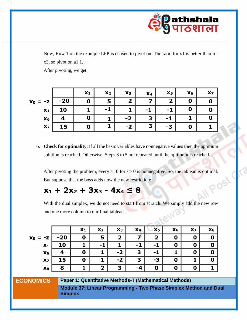
Now, Row 1 on the example LPP is chosen to pivot on. The ratio for x1 is better than for

x3, so pivot on a1,1.

After pivoting, we get

6. Check for optimality: If all the basic variables have nonnegative values then the optimum

solution is reached. Otherwise, Steps 3 to 5 are repeated until the optimum is reached.

After pivoting the problem, every ai, 0 for i > 0 is nonnegative. So, the tableau is optimal.

But suppose that the boss adds now the new restriction:

With the dual simplex, we do not need to start from scratch. We simply add the new row

and one more column to our final tableau.

____________________________________________________________________________________________________

ECONOMICS



13

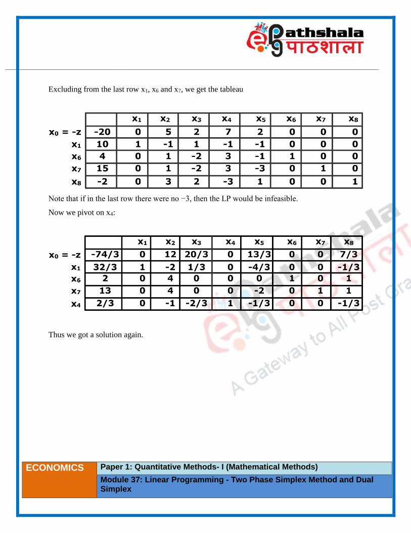
Excluding from the last row x1, x6 and x7, we get the tableau

Note that if in the last row there were no −3, then the LP would be infeasible.

Now we pivot on x4:

Thus we got a solution again.

____________________________________________________________________________________________________

ECONOMICS



14

5. Summary

Now let us summarize what we have learnt in this module, we have

The two phases of Simplex Method

Applications of Two-Phase Simplex Method

Learn Dual Simplex Method

Found out the difference between Dual Simplex and Simplex Method.

Documents

ECONOMICS Paper 1: Quantitative Methods- I (Mathematical