Study into Spectrally Efficient Radar Systems - Stakeholders - Ofcom

UNRESTRICTED

Study into Spectrally Efficient Radar Systems in the L and S BandsOfcom Spectral Efficiency Scheme 2004 - 2005 (SES-2004-2) 251

6 References

[1] The Report of an Investigation into the Characteristics, Operation and Protection Requirements of Civil Aeronautical and Civil Maritime Radar Systems, Radiocommunications Agency Final Report for Contract No AY4051 (AMS), October 2002 A Study into Techniques for Improving Radar Spectrum Utilisation, Ofcom Study Report No. AY4490 (Qinetiq), April 2004 Assessment of the Technical, Regulatory and Socio-economic Constraints and Feasibility of the Implementation of More Spectrally Efficient Radiocommunications Techniques and Technology within the Aeronautical and Maritime Communities, Ofcom Study Report No AY4620 (InterConnect Communications). June 2004

[4] CAP 670 Air Traffic Services Safety Requirements, Safety Regulation Group, CAA, http://www.caa.co.uk/docs/33/cap670.pdf

[2]

[3]

[5] Lamont V. Blake, ‘Radar Range-Performance Analysis’, Lexington Books 1980, ISBN 0-669-00781-1

[6]

ITU-R Recommendation P.838-2, Specific Attenuation Model for Rain for Use in Prediction, ITU-R, Geneva 2003 David K. Barton, ‘Modern Radar System Analysis, Artech House Inc, 1988, ISBN 0-89006-170-X

[10] http://www.metoffice.com/climate/uk/extremes/index.html

ITU-R Recommendation P.676-5, Attenuation by Atmospheric Gases, ITU-R, Geneva 2001

[7]

[8]

[9] R.G. Howell and P.A. Watson, “Rainfall Intensity Data for use in Prediction of Attenuation on Terrestrial Fixed Links”, Final Report for the Radiocommunications Agency under Research Contract AY 3362, June 2001

[11] M.W. Long, “Radar Reflectivity of Land and Sea”, (3rd Ed.), Artech House [12] Merrill I. Skolnik, Introduction to Radar Systems, International Student Edition,

McGraw-Hill Book Company, Inc., ISBN 0-07-057909-1 [13] ‘Guidelines for limiting exposure to time-varying electric, magnetic, and

electromagnetic fields (up to 300 GHz)’, International Commission on Non-Ionizing Radiation Protection, Health Physics April 1998, Volume 74, Number 4: 494-522.

[14] AC/AMJ 20.1317 Draft Final Issue (EEHWG Document WG327 dated November 98)

UNRESTRICTED Use, duplication or disclosure of data contained on this sheet is subject to the restrictions on the title page of this document

UNRESTRICTED

Study into Spectrally Efficient Radar Systems in the L and S Bands 252 Ofcom Spectral Efficiency Scheme 2004 - 2005 (SES-2004-2)

[15] John Holloway, ‘Design considerations for adaptive active phased array ‘multifunction’ radars’, Electronics & Communication Engineering Journal, pp227-288, December 2001

[16] Fred E. Nathanson, ‘Radar Design Principles - Signal Processing and the Environment’ (2nd Edition), SciTech Publishing, 1999

[18]

[38] http://www.02.com/media/speeches_040510a.asp

[17] RA Economic Impact report of 2002 Review of Radio Spectrum Management by Martin Cave, March 2002

[19] Reassessing the Diamond_Mirrlees Efficiency Theorem - Peter J. Hammond, March 2000

[20] Independent and Interconnect - Spectrum Issues for Mobile phone operators in India, July 2004

[21] Spectrum Pricing Third Stage Update and Consultation RCA, Dec 2002 [22] Economics of pricing Radio Spectrum – Chris Doyle/Martin Cave, March 2004 [23] ITU – Spectrum Management for a Converging World: Case Study on the United

Kingdom [24] The Economics of Radio Spectrum – Steve Jones, Paul LevineII, Neil Rickman,

Surrey University, Dec 2003 [25] Radio Technology and Research Second Annual Review, 2002 [26] ITV Written Evidence against Cave report [27] Economics of Spectrum Pricing Warwick- Dr Chris Doyle, Jan 2004 [28] Intellect Response to Ofcom Spectrum Trading Consultation, Nov 2003 [29] TERI Spectrum Pricing [30] Ofcom spectrum pricing, Sept 2004 [31] Indepen, Aegis systems and Warwick Business School - Spectrum pricing, Feb

2004 [32] RA - Strategy for the future use of the Radio Spectrum in the UK, 2002 [33] RA - Implementing Spectrum Trading, July 2002 [34] CEPT – Cost allocation and accounting systems used to Finance the Radio

Administration in CEPT Countries, Sept 2004 [35] Ofcom Spectrum framework review plan, Jan 2005 [36] C4 response to Ofcom Spec Pricing AIP [37] Economic Impact of Radio report by RA, 2001

[39] M. Cave and Audit Team, “Independent Audit of Spectrum Holdings”, HM Treasury, ISBN 1-84532-110-3: or via http://www.spectrumaudit.org.uk/pdf/caveaudit.pdf

[40] IEEE Standards Association via http://standards.ieee.org/getieee802/help.html[41] S M Mishra, D Cabric, C Chang∗, D Willkomm, B van Schewick, A Wolisz and R

W Brodersen,”A Real Time Cognitive Radio Testbed for Phy and Link Layer Experiments”, Proceedings of IEEE Symposium on New Frontiers in Dynamic Spectrum Access Networks (Dyspan’05), Baltimore 2005, pp 562 – 567, 2005


UNRESTRICTED


[42] “Spectrum policy task force report”, Federal Communications Commission, Tech. Rep. No. 02-155, Nov 2002

[43] S Haykin, K Huber and L Jiang, “Cognitive Radio” [44] A Sahai, “Some Fundamental Limitations for Cognitive Radio” BWRC Cognitive

Radio Workshop [45] J Mitola III, “Cognitive Radio: An Integrated Agent Architecture for Software

Defined Radio”, D. Tech. Dissertation, Royal Institute of Technology (KTH) Teleinformatics, Sweden, ISSN 1403-5286, May 2000.

[46] J Mitola III and G Q Maguire, “Cognitive Radio: making software radios more personal”, IEEE Personal Communications Journal, Vol. 6, No 4, pp13-18, 1999.

[47] S. Haykin, “Cognitive Radio: Brain empowered wireless communications”, IEEE JSAC, Vol. 23, No 2, pp2012-220, 2005.

[48] D. Cabric, S. M. Mishra, D. Willkomm, R. W. Broderson, and A. Wolisz, “A cognitive radio approach for usage of virtual unlicensed spectrum,” in 14th IST Mobile Wireless Communications Summit 2005, Dresden, Germany, June 2005.

[49] J Lansford, “UWB coexistence and cognitive radio”, Proceedings of IEEE International Workshop on Ultra Wideband Systems, (joint with Conference on Ultrawideband Systems and Technologies), pp35-39, 2004

[50] J R Foerster, ”Interference modelling of pulse-based UWB waveforms on narrowband systems”, Proceedings of 55th IEEE Vehicular Technology Conference, Vol. 4, pp 1931 – 1935, 2002.

[51]

[55]

M Welborn, “UWB Coesistence Issues”, Technical paper for IEEE 802.15-02/467r0.

[52] N S Correal, S Kyperountas, Q Shi and M Welborn, “An UWB relative location system”, Proceedings of IEEE Conference on Ultra Wideband Systems and Technologies, pp 394-397, 2003.

[53] R F Ormondroyd, “Spread-spectrum communication in the land mobile service”, IEE Conference Publication COM’78, No. 162, p 156-162, 1978.

[54] R F Ormondroyd and M S Shipton, “Spread spectrum communication systems for the land mobile service”, IERE Conference Proceedings on Land Mobile Radio, No 44, p 273-287, 1979. R F Ormondroyd and M S Shipton, “Feasibility of using spread-spectrum communication systems for the land mobile service on a non-interference basis with other users”, IERE Radio and Electronic Engineer, Vol. 50, No 8, pp 407-418, 1980.

[56] M S Shipton and R F Ormondroyd, “Improvements in use of congested spectrum for the land mobile radio service by adoption of bandsharing spread-spectrum system with TV broadcast channels”. IEE Proceedings F (Communications, Radar and Signal Processing), Vol. 128, No. 5, pp 245-60, 1981.

[57] R F Ormondroyd and M S Shipton, “Subjectively assessed impairment of television signals by co-channel operation of spread-spectrum radio systems”, IERE Conference Proceedings on Electromagnetic Compatibility, No. 56, pp 31-47, 1982.


UNRESTRICTED


[58] A E E Rogers, J E Salah, D L Smythe, P Pratap, J C Carter and M Derome, “Interference temperature measurements from 70 to 1500 MHz in suburban and rural environments of the Northeast”, Proceedings of 1st International Symposium on New Frontiers in Dynamic Spectrum Access Networks (DySPAN), pp 119- 123, 2005

[59] S M Cherry, “More air for Wi-Fi?”, IEEE Spectrum, Vol 40, Issue 2, p51, 2003.� [60] D M Febus, “An Interference Temperature Model for Improving Spectrum

Access” presented at 2005 IREAN Research Workshop [61] T C Clancy and W A Arbaugh, “Iterative Techniques for Interference

Temperature Measurement”, [62] T C Clancy and W A Arbaugh, “Stochastic Analysis of the Interference

Temperature Model” [63] H Kauppinen, “Spectrum Sharing and Flexible Spectrum Use”, Proceedings of

the XXIX URSI Convention on Radio Science, 1st November 2004. [64] S. B. Weinstein and P. M. Ebert, “Data transmission by frequency division

multiplexing using the discrete Fourier transform,” IEEE Trans. on Comms., Vol. COM-19, No. 5, pp.628-634, 1971.

[65] R. W. Chang and R. A. Gibby, “A theoretical study of performance of an orthogonal multiplexing data /transmission scheme”, IEEE Trans. on Comms., Vol. COM-16, No. 4 1968.

[66] B. Hirosaki, “An Orthogonal multiplexing QAM system using the discrete Fourier transform,” IEEE Trans. On Comms., Vol. COM. 29, No. 7, pp. 982-898, 1981.

[67] Alard, M and Lassalle, R; “Principles of modulation and channel coding for digital broadcasting for mobile receivers”; EBU Review, Tech. No. 224, pp. 47-69, August 1987.

[68] L. J. Cimini, “Analysis and simulations of a digital mobile channel using orthogonal frequency division multiplexing,” IEEE Trans. on Comms., Vol. COM-33, No. 7, 1985.

[69] F. Poegel, S. Zeisberg and A. Finger, “Comparison of different coding schemes for high bit rate OFDM in a 60 GHz environment”, Conf. Proc. IEEE ISSSTA’96, pp. 122-125, 1996.

[70] J Chiang aand R Lansford, “Use of cognitive radio techniques for OFDM ultrawideband coexistence with WiMax”, Texas Wireless Symposium pp 91-95, 2005.

[71] R F Ormondroyd and E A Al Susa, “Impact of multipath fading and partial-band interference on the performance of a COFDM/CDMA modulation scheme for robust wireless communications, IEEE Military Communications Conference. Proceedings. MILCOM 98, Vol.2, No 2, pp 673-678 1998.

[72] Scott Seidel, “IEEE 802 Tutorial – cognitive radio”, July 18, 2005 [73] http://www.ieee802.org/802_tutorials/july05/IEEE%20802%20CR%20Tutorial%2

07-18-05%20seidel%20input.pdf [74] C. Hwang and A. Syeed, Multiple Objective Decision Making – Methods and

Applications, Springer-Verlag, New York, 1979.


UNRESTRICTED


[75] C. M. Fonseca and P. J. Fleming, “Genetic Algorithms for multiobjective optimization: formulation, discussion, and generalization,” Proc. Int. Conf. Genetic Algorithms, pp. 416– 423, 1993.

[76] H. Lu and G. G. Yen, “Multiobjective optimization design via genetic algorithm”, IEEE Proc. International Conference on Control Applications, pp. 1190 – 1195, Sept. 2001.

[77] T. W. Rondeau, C. J. Rieser, B. Le, and C. W. Bostian, “Cognitive Radios with Genetic Algorithms: Intelligent Control of Software Defined Radios,” Proc. Of Software Defined Radio Conference, SDR’04, Phoenix, pp. C-3 –C-8. 2004

[78] R Montemanni, J N J Moon and DH Smith, “An improved tabu search algorithm for the fixed-spectrum frequency-assignment problem”, IEEE Transactions of Vehicular Technology, Vol. 52, No. 4, pp891 – 901, 2003.

[79] G Wyman, G R Bradbeer, S Hurley, R Taplin and D H Smith, “Improving efficiency in frequency assignment engines”, Proceedings of IEEE Military Communications Conference, 2001 (MILCOM 2001), Vol. 1, pp 25 - 29 2001

[80] A Capone and M Trubian, “Channel assignment problem in cellular systems: a new model and a tabu search algorithm”, IEEE Transactions on Vehicular Technology, Vol. 48, No. 4, pp 1252-1260, 1999.

[81] M Williams, “Making the best use of the airways: an important requirement for military communications”, IEE Electronics & Communication Engineering Journal, Vol. 12, No. 2, pp 75-83, 2000.

[82] L Berlemann, G R Hiertz, B Walke and S Mangold, “Cooperation in radio resource sharing games of adaptive strategies”, Proceedings of 60th IEEE Vehicular Technology Conference, (VTC2004-Fall), Vol. 4, pp 3004 – 3009, 2004.

[83]

[84]

J J Maxey ad R F Ormondroyd: "A downlink and uplink performance comparison of multi-carrier DS-CDMA using coding and interference cancellation", Proceedings of 2nd OFDM-Fachgespräch in Braunschweig, 1997.

J Neel, R Menon, J H. Reed and A B. MacKenzie, “Using Game Theory to Analyze Physical Layer Cognitive Radio Algorithms”, http://quello.msu.edu/conferences/spectrum/papers/neel-reed-menon-mackenzie.pdf S. Kaiser, S; “OFDM-CDMA versus DS-CDMA: Performance Evaluation for Fading Channels”; IEEE International Conference on Communications (ICC’95), pp. 1722-1726, June 1995.

[85] N. Yee, J. P. Linnartz and G. Fettweis, “Multi-carrier CDMA in indoors wireless networks,” Conf. Proc. IEEE PIMRC’93, pp. 109-113, Yokohama, Japan, 1993.

[86] K. Fazal and L. Papke, “On the performance of convolutionally coded CDMA/OFDM for mobile communication systems,” Conf. Proc. IEEE PIMRC’93, pp. 468-472, Yokahoma, Japan, 1993.

[87]

[88] K Challapali, S Mangold and B Dong, “Cognitive/spectrum-agile radios”, IEEE 802.11 Wireless Networks Group, working document 802.11-04-1472-00-0wng

[89] X Yiping, R Chandramouli and S Mangold, ”Dynamic spectrum access in open spectrum wireless networks”, IEEE Journal on Selected Areas in Communications, Vol. 24, No. 3, pp 626-637, 2006 Page(s):626 - 637


UNRESTRICTED


[90] “Radar handbook”, Merrill I Skolnik, 2nd ed. McGraw-Hill, 1990 [91] “Introduction to airborne radar”, GW Stimson, 2nd ed., SciTech Publishing, 1998

[100]

[103]

Proposal for a Study into Spectrally Efficient Radar Systems in the L and S Bands, 2004

[92] “A study into techniques for improving radar spectrum utilisation”, S.T. Ascroft, Qinetiq, Apr. 2004

[93] “Target tracking using television-based bistatic radar”, P E Howland, IEE proceedings Radar, Sonar and Navigation, 146(3) 166-174 1999.

[94] “Elementary mathematical and computational tools for electrical and computer engineers using MATLAB”, J.T. Manassah, CRC Press, 2001

[95] “Radar systems analysis and design using MATLAB”, B.R.Mahafza, Chapman & Hall / CRC, 2000

[96] “Utrawide-band coherent processing”, K.M. Cuomo - J.E. Piou - J.T. Mayhan, IEEE transactions of antennas & propagation, vol.47, No.6, June 1999

[97] “Radar target identification using one-dimensional scattering centres”, K.T. Kim, D.K. Seo, H.T. Kim,

[98] IEE proceedings on-line No.20010473, 2000 [99] “Digital Signal Processing using MATLAB”, V.K.Ingle – J.G.Proakis, PWS, 1997

“High range resolution using mono-frequency pulsed radar for the identification of approaching targets using subsampling and the MUSIC algorithm”, Dominic Grenier, IEEE Signal Processing letters, Vol.1, No.6, June 1996

[101] “Modern spectral estimation, theory and application”, S.M.Kay, Prentice Hall, 1988

[102] “High resolution radar imagery of the Mirage III Aircraft”, A.Zyweck – E.Bogner, IEEE transactions of antennas & propagation, vol.42, No.9, September 1994 “Radar target classification of commercial aircraft”, A.Zyweck – E.Bogner, IEE proceedings Radar, Sonar and Navigation.

[104] “HRR target recognition using the geometry information of scattering centres”, Zhang Xun – Zhuang Zhaowen – Guo Guirong, IEEE transactions of antennas & propagation.

[105] “Superresolution techniques for time-domain measurements with a network analyzer”, H. Yamada, M. Ohmiya, Y. Ogawa, and K. Itoh, IEEE transactions of antennas & propagation, vol.39, pp177-183, June Feb.1999

[106]

[107] Watchman TWT specification [108] F. H. Raab et al, ‘RF and Microwave Power Amplifier and Transmitter

Technologies – Part 1,’ High Frequency Electronics, May 2003, pp22-36 [109] F. H. Raab et al, ‘RF and Microwave Power Amplifier and Transmitter

Technologies – Part 2,’ High Frequency Electronics, July 2003, pp22-36 [110] F. H. Raab et al, ‘RF and Microwave Power Amplifier and Transmitter

Technologies – Part 3,’ High Frequency Electronics, September 2003, pp34-48 [111] F. H. Raab et al, ‘RF and Microwave Power Amplifier and Transmitter

Technologies – Part 4,’ High Frequency Electronics, November 2003, pp38-49


UNRESTRICTED


[112] F. H. Raab et al, ‘RF and Microwave Power Amplifier and Transmitter Technologies – Part 5,’ High Frequency Electronics, January 2004, pp46-54

[113]

R. Richardson, Case for a Coax, TN/81/2016, Marconi Radar Systems Ltd.

Euclid Contract no.01/EF1.14/012 on Spectrum Occupancy (SPECTROC) between the Western European Union (WEU) represented by the WEAO Cell (Contracting Authority) and THALES Air Defence S.A, (Contractor), Work Package 1 Final Report, 15th August 2002

S Bruss, ‘Linearization Methods’, April 23 2003 [114] K Mekechuk et al, ‘Linearization Power Amplifiers using Digital Predistortion,

EDA Tools and Test Hardware, High Frequency Electronics, April 2004, pp18-29.

[115] G. W. Orwell, Radar Transmitters [116] [117] Watchman Radar Specification, Air Surveillance Radar System, RSL 2736, Issue

5A, Plessey UK Limited, Radar Division, July 1986 [118] Unnecessary Sideband Emissions From Primary Radars and Options For Their

Control, Radio Communication Study Groups, 1998-2000, US1-5/61 Rev 2, 24 June 1999

[119]

[120] Euclid Contract no.01/EF1.14/012 on Spectrum Occupancy (SPECTROC) between the Western European Union (WEU) represented by the WEAO Cell (Contracting Authority) and THALES Air Defence S.A, (Contractor), Work Package 2 Final Report, 18th November 2002

[121] D G Manolakis, V K Ingle and S M Kogon, “Statistical and Adaptive Signal Processing”, McGraw Hill International Edition, Boston, 2000

[122] L C Godara, “Applications of antenna arrays to mobile communications, Part II: Beamforming and direction of arrival considerations”, Proc. IEEE, Vol. 85, No. 8, pp1195-1245, 1997

[123] B. Widrow, P E Mantey, L J Griffiths and B B Goode, “Adaptive Antenna Systems” Proc. IEEE, Vol. 55, No 12, pp 2143-2159, 1967

[124] J. Litva and T. Kwok-Yeung Lo, “Digital beamforming in wireless communications”, Artech House, London, 1996

[125] J.E Hudson, “Adaptive Array Principles”, Peter Perigrinus Ltd, London, 1981 [126] F. Harris, “On the use of windows for harmonic analysis with a discrete Fourier

transforms”, Proc. IEEE, Vol. 66, No. 1, pp51-83,1978 [127] J. Capon, “High resolution frequency-wavenumber spectrum analysis”, Proc

IEEE, Vol. 57, pp 1408-1418, 1969 [128] V.F. Pisarenko, “The retrieval of harmonics from a covariance function”,

Geophysical J. Royal, Astro. Soc., Vol 33, pp 347-366,1973 [129] R. O. Schmidt, “Multiple emitter location and signal parameter estimation”, Proc,

RADC Spectral Estimation Workshop, pp243-258, 1979 [130] R. Schmidt, “Multiple emitter location and signal parameter estimation”, IEEE

Trans. Antennas and Propagation, Vol 34, pp267-290, 1986


UNRESTRICTED


[131] G. Bienvenu and L. Kopp, “Optimality of high resolution array processing using the eigen system approach”, IEEE Trans. Acoustics, Speech and Signal Processing, Vol. 31, No 10, pp1235-1248, 1983

[132] I. Jami and R F Ormondroyd, “Estimation of the scattering radius around a mobile handset using sub-space methods”, Proceedings of the IEEE Eurocom 2000 Conference, pp 131-135, 2000

[133] A.J. Barabell, “Improving the resolution performance of eigenstructure based direction finding algorithms”, IEEE Conf. Proc. on ICASSP, 336-339, 1983

[134] B.D. Rao and K.V.S. Hari, “Performance analysis of root-MUSIC”, IEEE Trans. Acoustics, Speech and Signal Processing, Vol. 37, No. 12, pp 1939-1949, 1989

[135] P. Stoica and A. Nehorai, “MUSIC, maximum likelihood, and Cramer-Rao bound”, IEEE Transactions, Acoustics, Speech and Signal Processing, Vol 37, No. 5 pp 720-741, 1989

[136] R. Kumaresan and D.W. Tufts, “Estimating the angles of arrival of multiple plane waves”, IEEE Trans. Aerospace and Electronic Systems, Vol. 19, No. 1, pp134-139, 1983

[137] M. Kaveh and A. Barabell, “The statistial performance of the MUSIC and minimum norm algorithms in resolving plane waves in noise”, IEEE Trans. Acoustics, Speech and Signal Processing, Vol. 34, No. 2, pp 331-341, 1986

[138] R. Roy, A. Paulraj and T. Kailath, “ESPRIT-a subspace rotation approach to estimation of parameters of cissoids in noise”, IEEE Trans. Acoustics, Speech and Signal Processing, Vol. 34, No. 4, pp 331-1342, 1986

[139] R. Roy and T. Kailath, “ESPRIT-estimation of signal parameters vi rotational invariance techniques”, IEEE Trans. Acoustics, Speech and Signal Processing, Vol. 37, No. 7, pp 984-995, 1989

[140] B. Otterson, M. Viberg and T. Kailath, “Performance analysis of the total least squares ESPRIT algorithm”, IEEE Trans. Signal Processing, Vol. 39, No. 5, pp 1122-1135, 1991

[141] M Haardt and J.A. Nossek, “Unitary ESPRIT: How to obtain increased estimation accuracy with a reduced computation burden”, IEEE Trans on Signal Processing, Vol. 43, No 5, pp 1232-1242, 1995

[142] M. Tschudin , C. Brunner, T Kurpjuhn, T. Haardt and J.A. Nossek, “Comparison between unitary ESPRIT and SAGE for 3D channel sounding”, IEEE Vehicular Technology Conference, VTC’99, Vol. 2, pp 1324-1329, 1999

[143] M. Pesavento, A. Gershman and M Haardt, “Unitary Root-MUSIC with a real valued eigendecomposition”, IEEE Trans. on Signal Processing, Vol. 48, No. 5, pp1306-1314, 2000

[144] A.B Gershman and M. Haardt, “Improving the performance of unitary-ESPRIT via pseudo-noise resampling”, IEEE Trans. on Signal Processing, Vol. 47, No. 8, pp2305-2308, 1999

[145] K. Al Midfa, G.V. Tsoulos and A. Nix, “Performance analysis of ESPRIT,TLS-ESPRIT and unitary –ESPRIT algorithms for DOA estimation in a W-CDMA mobile system”, Conf. Proc. 1st Int. Conf. On 3G Mobile Communication Technologies, pp 200-203, 2000


UNRESTRICTED


[146] R.G. Stansfield, “Statistical theory of DF fixing”, Proceedings of the IEE, Vol. 14, part 3A, pp 762-770, 1947

[147] H.H. Jenkins, “Small aperture radio direction finding”, Artech House, Norwood, MA, 1991

[148] M. Gavish and E. Fogel, “Effect of bias on bearing-only target location”, IEEE Transactions on Aerospace and Electronic Systems, Vol. AES-26, No. 1, pp 22-26, 1990

[149] R.G. Wiley, “Electronic intelligence: the interception of radar signals”, Artech House, Dedham, MA, 1985

[150] P.J.D. Gething, “Radio direction finding and super-resolution”, 2nd Ed., Peter Perigrinus, London, 1991

[151] R.A. Poisel, “An introduction to communication electronic warfare systems”, Artech House, Norwood MA, 2002

[152] J.A. Cadzow, “Signal processing via least-squared error modelling”, IEEE ASSP Magazine, October, pp 12-31, 1990

[153] G.H. Golub amd C.F. Van Loan, “An analysis of the total least squared problem”, SIAM Journal of numerical analysis, Vol. 17, pp. 883-893, 1995

[154] K.D. Rao and D.C. Reddy, “A new method for finding electromagnetic emitter location”, IEEE Transactions on Aerospace and Electronic Systems, Vol. AES-30 No 4. pp 1081-1085, 1994

[155] R.M. Brown, “Emitter location using bearing measurements from a moving platform”, NRL Report 8483, Naval Research Laboratory, Washington, 1981

[156] R.E. Kalman, “A new approach to linear filtering and prediction problems”, Transactions of the ASME – Journal of basic engineering, Vol. 82 (Series D), pp 35-45

[157] V. Aidala, “Kalman filter behaviour in bearing-only tracking applications”, IEEE Transactions on Aerospace and Electronic Systems, Vol AED-15, No. 1, pp 29-39, 1979

[158] K. Spingarn, “Passive position location estimation using the extended Kalman filter”, ibid, Vol. AES-23, No. 4, pp558-567, 1987

[159] S. Challa and F.A. Farugi, “Non-linear system/linear measurement approach to passive position location using extended Kalman filtering”, IEEE TENCON – Digital Signal Processing Applications, pp. 665-669, 1996

[160] T.L Song and J.L. Speyer, “A stochastic analysis of a modified gain extended Kalman filter with application to estimation of bearings-only measurements”, IEEE Transactions on Automatic Control, Vol. AC-30 No. 10, pp. 940-949, 1985

[161] S.J. Julier and J.K. Uhlman, “A new extension of the Kalman filter to non-linear systems”, Proc. 11th Int Symposium on Aerospace/Defense Sensing, Simulation and Control, 1997

[162] D.S. Elsaesser and R.G. Brown, “The discrete probability density method for emitter geolocation”, Technical Memorandum No 2003-068, DRDC, Canada. 2003

[163] W.H. Foy, “Position-location solutions by Taylor –series estimation”, IEEE Transactions on Aerospace and Electronic Systems, Vol. AES-12, No. 2, pp 187-193, 1976


UNRESTRICTED


[164] P.I. Rusu, “A TOA_FOA solution for the position and velocity of RF emitters”, Applied Research Laboratories Report, #SGL-GR-99-15, The University of Austin Texas

[165] N. Levanon, “Interferometry against differential Doppler: Performance comparison of two emitter location airborne systems”, IEE Proceedings, Vol. 136, Pt F, No. 2, pp70-74, 1989

[166] R.K. Otnes, “Frequency difference of arrival accuracy”, IEEE Transactions on Acoustic, Speech and Signal Processing, Vol. 37, N0.2, pp306-308, 1989

[167] D-H Shin and T-K Sung, “Comparison of error characteristics between TOA and TDOA positioning”, IEEE Transactions on Aerospace and Electronic Systems, Vol. AES-38, No.1 pp. 307-310, 2002

[168] J.D. Bard, F.M. Ham and W.L. Jones. “An algebraic solution to the time difference of arrival equations”, Proc. SouthEastcon Conference, Tampa, pp 313-319, 1996

[169] J.D. Bard, F.M. Ham and W.L. Jones. “Time difference of arrival dilution of precision and applications”, IEEE Transactions on Signal Processing, Vol. 47, No. 2 pp 521-523, 1999

[170] G.M, Pachter, and J. Raquet, “Closed-form solution for determining emitter location using time difference of arrival measurements”, IEEE Transactions on Aerospace and Electronic Systems, Vol. AES-39, No. 3 pp. 1056-1058, 2003

[171] K.F. McDonald and W.S. Kuklinski, “Track maintenance and positional estimation via ground moving target indicator and geolocation data”, Conference Proceedings of IEEE Radar 2001, pp. 239-244, 2001

[172] D.J. Torrieri, “Statistical theory of passive location systems”, IEEE Transactions on Aerospace and Electronic Systems, Vol. AES-20, No. 2, pp.183-198, 1984

[173] BBC Digital radio transmitter sites, see http://www.bbc.uk/reception/radio_transmitters/digital_radio.shtml

[174] Nicholas J Willis, “Bistatic radar”, Artech House, 1991, ISBN 0-89006-427-X. [175] Michael R. B. Dunsmore, ’Chapter 11 Bistatic Radars’ see ‘Advanced Radar

Techniques and Systems, Ed Gaspare Galati, IEE publishing [176] I. Papoutsis, C.J. Baker, H.D. Griffiths, ‘Netted radar and The Ambiguity

Function’, 2nd EMRS DTC Technical Conference – Edinburgh 16th-17th June 2005.

[177] Special Issue: Passive Radar Systems, IEE Proceedings Radar, Sonar & Navigation, Volume 152 Number 3 June 2005, ISSN 1350-2395

[178] Pytor Y. Ufimtsev, “Comments on the Diffraction Principles and Limitations of RCS Reduction Techniques”, Proceedings of the IEEE, Vol. 84, No 12, December 1996, pp1830-1851.

[179] J.I. Glaser, “Bistatic RCS of Complex Objects Near Forward Scatter”, IEEE Trans AES-21, 70-78 Jan 1985.

[180] P.E. Howland, “Passive tracking of airborne targets using only Doppler and DOA information”, IEE Colloquium Digest No. 1995/104, pp7/1-3, May 1995.

[181] Elliott D Kaplan, ‘Understanding GPS Principles and Applications’, Artech House Inc., 1996, ISBN 0-89006-739-7.


UNRESTRICTED


[182] FAA ADS-B Home page, see http://adsb.tc.faa.gov/ADS-B.htm [183] ‘Transponder drop-outs spark AD’, David Learmont, Flight International,

02/08/05, see: http://www.flightinternational.com/Articles/2005/08/02/200673/Transponder+drop-outs+spark+AD.html

[184] C.J. Baker, H.D. Griffiths, I. Papoutsis, “Passive Coherent Location Radar Systems Part 2: Waveform properties”, P160-168, IEE-Proc. Radar Sonar Navigation, Vol. 152, No.3, June 2005

[185] The CAPANINA project, see http://www.capanina.org/overview.php [186] BBC Digital radio transmitter sites, see

http://www.bbc.uk/reception/radio_transmitters/digital_radio.shtml


UNRESTRICTED

Study into Spectrally Efficient Radar Systems in the L and S BandsOfcom Spectral Efficiency Scheme 2004 - 2005 (SES-2004-2) A-1

Annex A Angle of Arrival Estimation Methods

A.1 Introduction There are a number of different methods of estimating the angles of arrivals (AOA) of multiple plane waves using an antenna array. Throughout this section it is assumed that the array is a uniform linear array (ULA), however, the techniques are applicable to other arrays, such as circular arrays, if the array response vector is known16. The methods are broadly categorised into (i) Fourier-based methods, which obtain the steered response of the antenna, (ii) parametric methods, which attempt to match the signals received on each antenna element to a particular far-field spatial distribution via a model of the far-field distribution and (iii) sub-space decomposition methods, such as Pisarenko’s method, MUSIC and ESPRIT and their numerous variants. This Annex provides a comparison of the main methods of estimating the AOA of multiple arriving signals. The performance of the various methods is compared using Matlab simulations that were carried out as part of this workpackage under a consistent set of conditions. Further information on these methods can be found in [1,2].

A.2 Signal Model Throughout this Appendix, it is assumed that the signal received by the antenna array comprises multiple, K, modulated sinusoidal carriers that each arrive from different angles of arrival. The ith signal has the form:

( ) ( ) K,, tftAts iicii ,21for 2cos)( Kαπ += (A.1)

where ( ) 1±∈tAi is the data modulation (assumed to be BPSK for simplicity), is the

carrier frequency and icf

iα is the random phase of the carrier when it arrives at the reference element of the antenna array. The frequencies of each carrier may be the same, , or they may be different, either due to the effect of different Doppler shifts at the different angles of arrival, or because they represent different source frequencies.

cf

16 The array response vector is sometimes known as the array manifold. It relates the electrical phase shift of the incoming (plane) wave front of the signal at each of the elements in the array due to the path length difference between the wave front and the array element. As such it relates the spacing and geometry of the array elements with the angle of arrival of the plane wave.


UNRESTRICTED

Study into Spectrally Efficient Radar Systems in the L and S Bands A-2 Ofcom Spectral Efficiency Scheme 2004 - 2005 (SES-2004-2)

For the most part, it will be assumed that the modulating signal is different for each user so that the various signals, although co-channel are uncorrelated. In some cases it will be assumed that the arriving signals are coherent. In this case, the data modulation and the carrier frequency is assumed to be identical for all signals at the different angles of arrival; however, the phase of each signal on arrival at the antenna is assumed to be different. This condition corresponds to the case of multipath reception from a single static source.

The output of the array, expressed as a vector, is given by:

( ) ( ) ( )ttt nVsx += (A.2)

where

⎥⎥⎥

⎦

⎤

⎢⎢⎢

⎣

⎡=

Kv

vV M

1

and is the (1×M) vector of signals on the M elements of the array for the signal sam ime t is the (1×K) vector of the signal samples at time t, V is the (K×M) array response matrix (where the ith row corresponds to the (1×M) array response vector

for the ith signal of frequency at an azimuth angle to the array of

( )txples at t , ( )ts

( )tivicf iφ and ( )tn is the

(1×M) vector of additive Gaussian noise samples at each element at time t. The additive noise may represent the normal additive noise processes found in all receivers, or it may additionally represent a spatially random signal due to interference.

A.3 Fourier-based methods Fourier-based methods [3,4,5] are the most robust method of AOA estimation, since they require no a priori information regarding the number, L, of co-channel signals that may impinge on the array (subject generally to the limit, 1−≤ ML , where M is the number of elements in the array).

Consider a plane wave arriving at an azimuth angle φ to the ULA, as shown in figure A.1.

d

1 2 3 M

dsinφ φ

Figure A-1 : Geometry used for the uniform linear array


UNRESTRICTED


The wavefront at two adjacent elements has a path length difference of cd φsin , and this results in an electrical phase shift of λφπθ sin2 d= between the two elements, where λ is the wavelength of the signal and d the spacing between antenna elements. The phase shift of the signal at the mth element relative to the first element (labelled 1 in figure A.1) is [1]:

( )λ

φπθ sin21 dmm −= (A.3)

and the corresponding array response vector for the ULA is:

( ) [ ]Tλφπλφπφ /sin2)1(/sin21 dMjdj ee −−−= Lv (A.4)

where []T represent transposition of the vector.

The antenna array can be seen as a method of spatially sampling wavefronts propagating at a particular carrier frequency. For the ULA, the ‘spatial sampling frequency’, , is given by:

sU

dU s

1= (A.5)

With temporal signals, the phase progression for uniform sampling is a consequence of the frequency; that is, consecutive unit time samples of the same signal differ only by a phase shift , where F is the frequency. For the case of a spatially propagating signal the phase progression is due to the distance propagated by the wavefront and this frequency is represented by the spatial frequency:

Fje π2

λφsin

=U (A.6)

and the normalised spatial frequency is:

λφsindu = (A.7)

Consequently, the array response vector can be written in terms of the normalised spatial frequency as:

( ) [ ]TuMjuj ee ππφ 2)1(21 −−−= Lv (A.8)

The inter-element spacing is the spatial sampling interval and similar to Shannon’s theorem for discrete-time signals, the normalised frequencies are unambiguous over the range

21

21

≤≤− u . Since the full range of possible unambiguous angles that can be detected by

the ULA is , this requires that: oo 9090 ≤≤− φ


UNRESTRICTED


2λ

≤d (A.9)

to prevent ambiguities in angle measurement over the full range. This analogy between time and frequency of temporal signals and spatial sampling and spatial frequency, explains how Fourier methods can be used to obtain the AOA of the signal.

The output of the array is the weighted sum of the signals received at each element:

( ) ( )nnxcyM

mmmn xcH=∑=

=1

* (A.10)

where * means conjugation, H means the Hermetian operation (conjugate transpose), is the nth sample of the sampled signal obtained at the mth array element and is

the complex valued weighting coefficient of the mth antenna element. Also, c is the vector of the weight coefficients and x(n) is the vector of the nth signal sample received at each element.

( )nxm mc

The array acts as a spatial matched filter when the weight coefficients are set equal the array response vector for a signal whose wavefront has an azimuth angle sφ to the array:

( ) ( )ssmf φφ vc = (A.11)

since in this case, the phase delay inserted by the spatial separation of the elements is perfectly compensated by the phase advance provided by the weights (hence the need for the conjugation operation in (A.10)). Consequently, the scalar output of the spatial matched filter is given by:

( ) ( ) ( ) ( ) (nny ssmfsn xvxc φφφ HH == )

It will be seen from (A.12), given the form of the steering vector given by (A.8), that the steered response of the spatial matched filter has precisely the same form as the discrete-time Fourier transform, in which spatial frequency replaces temporal frequency. This function is continuous in spatial frequency.

Suppose that we do not know the direction of the signal. One method is to repeatedly change the look direction, φ, used for the array response vector and for each value of φ obtain the corresponding output of the array for that direction using (A.12). This is called the steered response of the array. In this case, the use of

(A.12)

( )φv in this way is referred to as a steering vector as it is used to point the array (via the array coefficients c) in a particular look direction. The maximum of the absolute value of the steered response will correspond to the situation where the look direction of the steering vector points to the true angle sφ of the wanted signal. An alternative form that can be used for AOA estimation is to use the spatial power response instead of the absolute value of the steered response, which is given by:

( ) ( ) ( ) ( ) ( ) ( )222 nnyC ssmfsn xvxc φφφφ HH === (A.13)


UNRESTRICTED


Since (A.12) and (A.13) are continuous in φ , the grid size used to select the various φ due to values can be extremely fine, although this is at the expense of computational effort

the calculation of a very large number of complex exponentials. A less computationally intensive approach is to compute the steered response vector at a finite number of discrete values of φ using the discrete Fourier transform17 in place of the discrete-time Fourier transform to obtain the spatial power response in terms of the spatial frequency, u:

( ) ( ) 2)(nxuC ℑ= (A.14)

and then to convert the spatial frequency to angle, φ , via:

⎟⎠⎞

⎜⎝⎛= −

duλφ 1sin (A.7)

However, consider the situation where the array has only eight elements. By directly applying the discrete Fourier transform to the eight sample values, , provides only eight corresponding points in both the spatial spectrum

. This is far too coarse to pinpoint the required AOA. The solution is to use the zero-padded FFT. This corresponds to the situation where the real array elements containing the signal samples x(n) are supplemented by many additional dummy elements whose signal samples are taken as zero. Consequently, 8 real sample values could be supplemented by 1016 dummy points (say) and the spatial power response computed using a 1024 point FFT algorithm giving a much finer spatial frequency response curve.

However, for realistically sized arrays, zero-padding does not

( )nx and the azimuth angle over the range

o90±

improve the angular resolution of the antenna array due to the fact that, because of the finite number of array elements, the steered response of the spatial matched filter beamformer produces a finite width main-lobe as well as sidelobes. Furthermore, because of the non-linear relationship between the spatial frequency and azimuth angle, the sidelobe structure is heavily distorted in terms of angle. The effect of the broad main lobe on accurate AOA estimation is felt particularly if the signal snapshot, x(n), is corrupted by noise, since the precise peak of the mainlobe, indicating the AOA, is determined by the noise corrupting that particular snapshot.

Figure A.2a shows the normalised steered response of an 8 element array to a single far-field source at an angle, to the array, using the geometry of figure A.1. In this case the frequency is chosen to be 1.5GHz and the antenna spacing at this frequency is chosen to be λ/2 (overall length of array, 1.6m). The signal is received in the absence of noise and in order to obtain this response, a 1024-point zero-padded FFT is used (i.e. 1016 inserted zeros). Note the beamwidth of the mainlobe and the sidelobes.

25= oφ

17 In practice, a fast Fourier transform algorithm would be used in place of the discrete Fourier transform as it is computationally less intensive but this places a restriction that the number of sample points used (including dummy zeros, if zero padded) is N=2n, where n is an integer..


UNRESTRICTED


Contrast this with the normalised steered response of a much larger, 32 element array (overall length of array 6.4m), as shown in figure A.2b, where, as expected, the width of the main lobe is much reduced.

(a) 8 Element ULA (b) 32 Element ULA

Figure A-2 : Steered response of an a linear array to a far field source at 25° using FFT method

Furthermore, even in the absence of noise, it may be very difficult to accurately resolve two or more signals arriving at different AOAs if they fall within the main lobe, particularly if one signal is much stronger than the other since the steered response is the convolution of the spatial matched filter beam pattern with the spatially separated sources, and the peak in the spatial power response may not correspond to the AOA of any of the signals! This problem is not confined to sources located within the main lobe. It is quite possible that a strong signal well separated from a weaker signal may produce sidelobes in the spatial power response that heavily distort the mainlobe peak of the weaker source, making it difficult to pinpoint the precise AOA. Figure A.3a and A.3b show the ability of the Fourier method to resolve two far-field sources at 25° and 35° in the absence of noise. A 1024 point zero-padded FFT is used to obtain this response. In this case it should be noted that the two signals are coherent (i.e. the data modulation for both signals is assumed to be identical and the two carrier frequencies are identical).

(a) 8 Element array (b) 32 Element array

Figure A-3 : Steered response of ULA for two far field sources at 25° and 35° using FFT method


UNRESTRICTED


It is possible to suppress the effect of the sidelobes, generally at the expense of further broadening the width of the main lobe, by using appropriate taper functions [6]. These taper functions, t, weight the signal sample snapshot, ( )nx in amplitude prior to the signals being weighted in phase by the beamformer coefficien the effective weights become

, where represents element by element multiplication. These amplitude weights are generally symmetrical about the central element(s) of the array with a maximum in the centre, tapering to a smaller value at each end of the array. The shape of the taper is generally smooth, such as a Gaussian-like shape or a raised cosine. There are many different types of taper function available, each providing different levels of sidelobe suppression and main-lobe broadening. A common taper is the Dolph-Chebyshev taper:

ts c, i.e. tcc ⊗=t ⊗

( ) ( )[ ]( ) ( )[ ]⎪⎩

⎪⎨⎧

>−≤−= −

−

12/cosfor 2/coscosh1cosh12/cosfor 2/coscos1cos)( 1

1

nnNCnnNCnt

ββββ (A.15)

where ( ) ( )[ ]αβ 05.011 10cosh1cosh −−−−= N and α is the sidelobe level needed in dB. This taper provides good general performance, but others include Hanning tapers, Hamming tapers and Kaiser tapers. A less good feature of the taper is that it reduces the spatial response of the beamformer to the wanted signal(s). Figure A.4 shows the impact of using the Dolph-Chebyshev taper with α=−3dB for the case of figure A.3a when the 8 element array was unable to resolve the two signal sources. Ironically, although this has appeared to increase the sidelobe level, it has improved resolution.

Figure A-4 : Use of the Dolph-Chebychev taper to help resolve the two far-field sources at 25° and 35°, which were not resolvable with the untapered 8 element ULA shown in figure A.3a

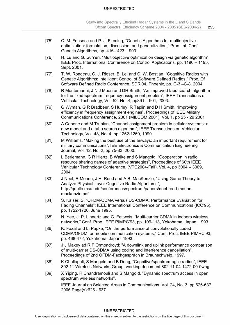
Invariably, the signal of interest will be corrupted by noise, and figure A.5a shows the effect of AWGN (receiver noise or clutter) at an SNR=10dB on the steered response for the 8 element ULA for a single far-field source at 25°. Shown in this figure are 10 snapshots of the steered response.


UNRESTRICTED


(a) (b)

Figure A-5 : Impact of a 10dB SNR on the steered response of the 8 element ULA to a single source at 25° (a) raw snapshots (b) averaged periodogram response after averaging 100 snapshots

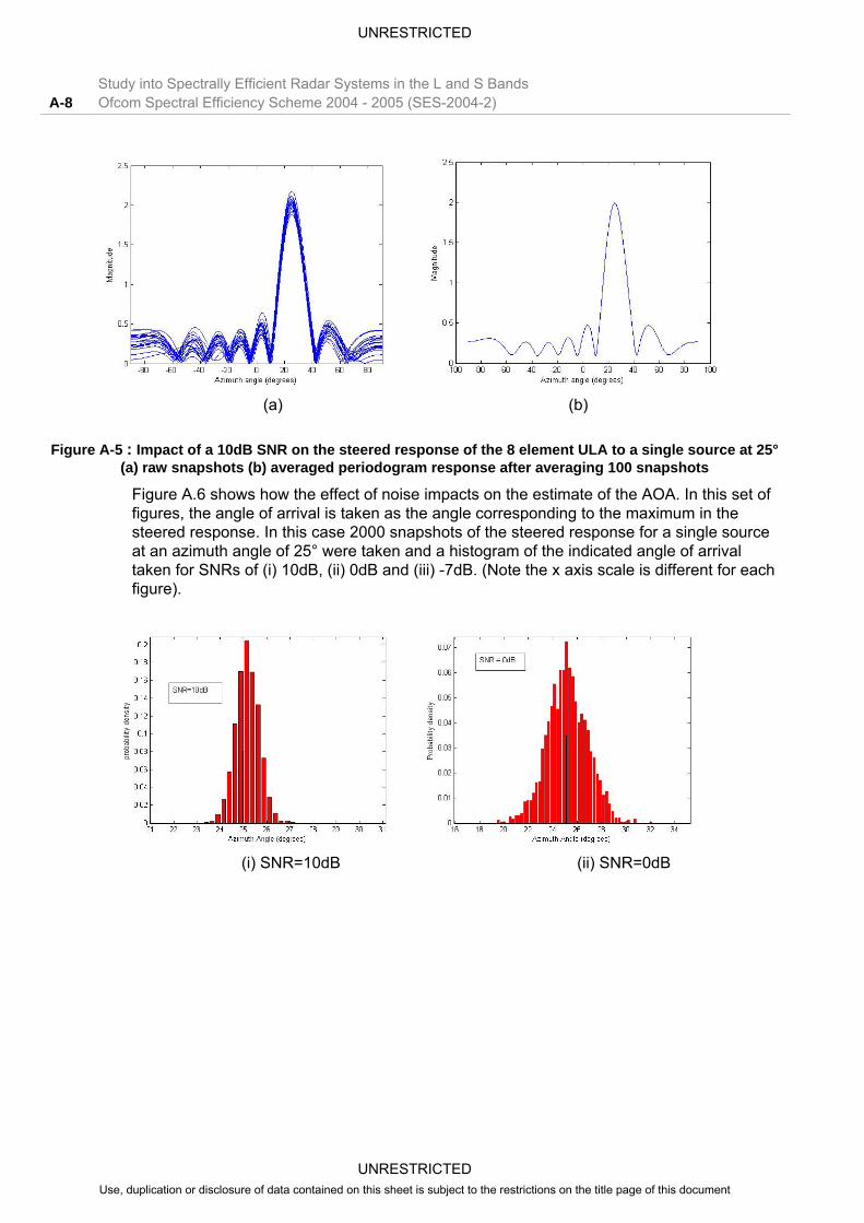
Figure A.6 shows how the effect of noise impacts on the estimate of the AOA. In this set of figures, the angle of arrival is taken as the angle corresponding to the maximum in the steered response. In this case 2000 snapshots of the steered response for a single source at an azimuth angle of 25° were taken and a histogram of the indicated angle of arrival taken for SNRs of (i) 10dB, (ii) 0dB and (iii) -7dB. (Note the x axis scale is different for each figure).

(i) SNR=10dB (ii) SNR=0dB


UNRESTRICTED


(iii) SNR = -7dB

Figure A-6 : Effect of SNR on the distribution of the measured angle of arrivals for the FFT method

One way of reducing the effect of the signal noise on the accuracy of the AOA spectrum is to use P snapshots of the array signal samples, ( ) ( )nn Pxx L,1 , and to use the averaged periodogram to obtain the average spatial power response ( )φC by performing P spatial power responses ( ( )φpC ) and to take the average of each spectral coefficient from the P values.

( ) ( )∑==

P

ppC

PC

1

1 φφ (A.16)

This approach is computationally intensive as it relies on taking P zero-padded FFTs of size N bins and then performing N averages, each containing P values. Nevertheless, it is effective, as figure A.5b shows for the case where P=100 snapshots were used in the averaging process. In this case, to the precision of a 1024 point FFT, even after 1000 tests, there was no error in estimating the correct AOA at an SNR=-7dB or better.

An alternative approach, which is generally less computationally intensive than the averaged periodogram, is to perform averaging first and then to take a single zero-padded FFT. In this case, the averaging takes the form of the spatial correlation of the signal samples across the antenna array. Spatial correlation represents how the average signal phase changes from one antenna element to the next. This information is provided by the spatial correlation function described in the next section

A.4 Spatial Correlation The samples of the signal at the individual elements represent a ‘snapshot’ of the variation of the phase across the array and each snapshot can be used to obtain the instantaneous AOA for those samples, as described above. However, since each signal sample is noisy the accuracy of the AOA estimate is degraded, since the noise samples transform into a noisy spatial power response. The array correlation matrix of the signal vector shows the individual correlations of the received signals between all the elements of the array

)(nx

[ ]HxxR Ex = (A.17)


UNRESTRICTED


where is the expectation operation. In this expression reference to the sample number n has been removed because the expectation is obtained from the long term average of a great many signal vector snapshots. The array correlation matrix has the form:

[ ]E

[ ] [ ][ ] [ ][ ] [ ] ⎥

⎥⎥⎥⎥⎥

⎦

⎤

⎢⎢⎢⎢⎢⎢

⎣

⎡

⎥⎦⎤

⎢⎣⎡

⎥⎦⎤

⎢⎣⎡

⎥⎦⎤

⎢⎣⎡

=

2*1

*

*2

22

*2

*1

*1

21

1

1

2

MM xExxExxE

xxExExxE

xxExxExE

M

M

M

L

MOMM

L

L

R (A.18)

In practice, the expectation of each element of R is approximated by average values obtained over an acceptably large number of samples, P, commensurate with the stationarity of the signal statistics

[ ] ( ) ( )∑≈=

P

njiji nxnx

PxxE

1

*1 (A.19)

In practice the two operations can be conveniently combined by storing the signal vector for P snapshots as a matrix, X:

( ) ( ) ( )( ) ( ) ( )

( ) ( ) (

( ) ( ) ( )⎥⎥⎥⎥⎥⎥⎥⎥

⎦

⎤

⎢⎢⎢⎢⎢⎢⎢⎢

⎣

⎡

+++

+++

+++

=

PnxPnxPnx

pnxpnxpnx

nxnxnxnxnxnx M

111

111

111

21111

L

MMMM

L

MMMM

L

L

X ) (A.20)

such that:

XXR HP1ˆ = (A.21)

This is a very straightforward operation. The hat signifies that the correlation matrix is an estimate rather than the true correlation matrix. However, it is important to recognise that the error in the estimate of R̂ , impacts on the accuracy of all the methods of spectrum estimation that rely on it.

Note that the correlation matrix is different from the correlation function since the latter obtains the overall correlation at a particular ‘lag’. So for example, the first term of the correlation function would comprise:

( ) ∑ ⎥⎦⎤

⎢⎣⎡=

=

M

iixE

MR

1

210ˆ (A.22)

the second term would comprise:


UNRESTRICTED


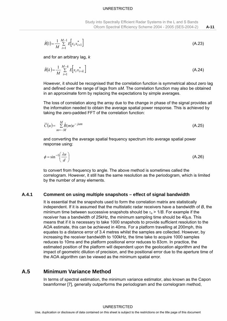
( ) [ ] (A.23) ∑=−

=+

1

1

*1

11ˆ M

iii xxE

MR

and for an arbitrary lag, k

( ) [∑=−

=+

kM

ikii xxE

MkR

1

*1ˆ ] (A.24)

However, it should be recognised that the correlation function is symmetrical about zero lag and defined over the range of lags from ±M. The correlation function may also be obtained in an approximate form by replacing the expectations by simple averages.

The loss of correlation along the array due to the change in phase of the signal provides all the information needed to obtain the average spatial power response. This is achieved by taking the zero-padded FFT of the correlation function:

( ) ∑=−=

−M

Mm

jumemRuC )(ˆ (A.25)

and converting the average spatial frequency spectrum into average spatial power response using:

⎟⎠⎞

⎜⎝⎛= −

duλφ 1sin (A.26)

to convert from frequency to angle. The above method is sometimes called the correlogram. However, it still has the same resolution as the periodogram, which is limited by the number of array elements.

A.4.1 Comment on using multiple snapshots – effect of signal bandwidth It is essential that the snapshots used to form the correlation matrix are statistically independent. If it is assumed that the multistatic radar receivers have a bandwidth of B, the minimum time between successive snapshots should be τs > 1/B. For example if the receiver has a bandwidth of 25kHz, the minimum sampling time should be 40µs. This means that if it is necessary to take 1000 snapshots to provide sufficient resolution to the AOA estimate, this can be achieved in 40ms. For a platform travelling at 200mph, this equates to a distance error of 3.4 metres whilst the samples are collected. However, by increasing the receiver bandwidth to 100kHz, the time take to acquire 1000 samples reduces to 10ms and the platform positional error reduces to 83cm. In practice, the estimated position of the platform will dependent upon the geolocation algorithm and the impact of geometric dilution of precision, and the positional error due to the aperture time of the AOA algorithm can be viewed as the minimum spatial error.

A.5 Minimum Variance Method In terms of spectral estimation, the minimum variance estimator, also known as the Capon beamformer [7], generally outperforms the periodogram and the correlogram method,


UNRESTRICTED


described in the previous section and it has the advantage that it uses the correlation matrix directly rather than the correlation sequence. It is often referred to as a high resolution spectral estimator and it also has the advantage that it is non-parametric, which means that it does not assume an underlying model, whose parameters need to be known a priori.

The minimum variance spectral estimate can be shown to be:

( )( ) ( )φφ

φvRv 1

ˆ−

=Hmv

MR (A.27)

where ( )φv is the steering vector at some azimuth angle φ. This means that the spectrum has to be obtained by forcing the look angle φ through all angles of interest. Figure

A.7 shows the equivalent steered response for the same 8 element array as for the previous examples for a single far-field source at an azimuth angle of 25° but using the minimum variance spectral estimator. As for the previous examples, the number of look angles is set at 1024, distributed over ±90°. It should be noted that the SNR of the signal at each element is 0dB prior to signal averaging. However, the estimated correlation matrix in this figure is produced by averaging over 500 signal vector snapshots.

( )φmvR̂

Figure A-7 : Equivalent steered response of an 8 element array to a single source at 25° using the minimum variance method at an SNR=0dB (500 snapshot averaging)

It is immediately clear why this is referred to as a high resolution method. Figure A.8a shows the same steered response estimator for three coherent signal sources located at -35°, +25° and +40° for the case where each signal is equal power and the SNR for each signal is 0dB. Although it appears from this figure that this estimator ought to able to resolve better than 15°, this is virtually the limit at this SNR. Shown in figure A.8b, is the situation where the three signals were not coherent (due to random data on each source. Again, 15° appears to be the limit of the resolution of this method for an 8 element array at an SNR=0dB per source, but with 500 snapshot averaging to form R̂ . However, if the number of elements is increased to 32, then the resolution is significantly improved, as shown in figure A.9 and it is able to resolve 4° source separation with ease, and 3° with more difficulty. In this figure, the sources are located at -35°, +25° and +29°. As before,


UNRESTRICTED


case (a) is for coherent sources and (b) is for non-coherent sources. Although the resolution is no higher for case (b) than case (a), the determination of the three AOAs seems to be much clearer for the non-coherent case.

(a) Coherent Sources (b) Non-coherent sources

Figure A-8 : Steered response of an 8 element array using the minimum variance method for signal sources at -35°, 25° and 40° at an SNR=0dB per signal source (500 snapshot averaging)

(a) Coherent sources (b) Non-coherent sources

Figure A-9 : Steered response of a 32 element array using the minimum variance method for signal sources at -35°, 25° and 29° at an SNR=0dB per signal source (500 snapshot averaging)

The major penalty of the minimum variance method is the need for significant averaging to produce the estimate of the correlation matrix R̂ . If this is not carried out, and the estimate of R̂ is poor, the estimate of the steered response is also extremely poor. As an example, figure A.10a shows the effect of using only 10 snapshots of the signal vector x even though the SNR is 10dB. The array had 8 elements and the three sources were located at -35°, 25° and 40°. Coherent sources were used to obtain this result. In this case, one wanted source is not detected and additional peaks which are extremely dependent on the noise, are observed. Figure A.10b shows the same case after 50 snapshots are used to form R̂ and figure A.10c after 100 snapshots are used.


UNRESTRICTED


(a) 10 snapshot averaging (b) 50 snapshot averaging (c) 100 snapshot averaging

Figure A-10 : Effect of amount of averaging to produce R̂ on the steered response for sources at -35°, 25° and 40° (for the case of coherent sources)

A.6 Super-resolution methods based on Eigen-decomposition Although Fourier-based methods are robust, the relatively low number of array elements that can be accommodated in practical arrays means that the broad main-lobe beamwidth of the steered response is a major limiting factor to the resolution of Fourier methods. When using array processing to obtain the AOA, we are attempting to identify the spatial frequency of the complex exponentials representing the phase shift of the wavefronts of the various signals as they propagate along the array. This is particularly true as long as the wavefront of each signal is flat when each wavefront corresponds to a single frequency complex exponential. Consequently, the method described in this section is based on a harmonic signal model and the method obtains the parameters (i.e. frequency) of the complex exponentials that form the basis of the method.

Unlike the Fourier methods where the signal is decomposed into N complex exponentials (or N/2 sinusoids/cosines) arranged on a fixed frequency interval on the basis of taking N sample values, here the signal is assumed to comprise of a limited number of complex exponentials whose frequencies must be evaluated. The advantage is that the frequency separation of these complex exponentials may be very close (much closer than the equivalent main lobe beamwidth of the Fourier methods). Consequently, these methods are often referred to as super-resolution methods. However, the success of these methods is very much dependent upon the accuracy of the underlying model. Consequently, if it is known that there are four signals at different AOAs, the model will find the parameters of four complex exponentials. If, in reality, there are only three signals but the model assumes four, four AOAs will be found(!), and it is not guaranteed that any of the frequencies found by the method will then be correct!

Eigen-methods of AOA determination (also known as subspace methods) also use the array correlation matrix as the starting point. However, in this class of methods, the array correlation matrix is decomposed into its eigenvalues and eigenvectors:

HQQΛR =ˆ (A.28)

where is an (M×M) diagonal matrix comprising the eigenvalues while Q is an (M×M) matrix whose columns, q1, …, qM are the corresponding eigenvectors.

Λ


UNRESTRICTED


[ ]MqqQ L1= (A.29)

It is assumed that each of the elements of the correlation matrix consist of a wanted term representing the degree of correlation between the elements and a noise term due to the limited averaging employed to obtain the correlation. It is assumed that the noise term is uncorrelated with the wanted signal. Eigen-decomposition allows the correlation matrix to be decomposed into a matrix representing the wanted terms and a matrix representing the noise terms:

HHHHnnsssnnnsss QQQΛQQΛQQΛQR 2σ+=+= (A.30)

where σ is the standard deviation of the noise.

These two sub matrices are called the wanted signal subspace and the noise subspace. It is important to recognise that the signal eigenvectors are orthogonal to the noise eigenvectors. Here, represents a (K×K) diagonal matrix of the K largest eigenvalues and represents a ((M-K)×(M-K)) diagonal matrix of the M-K smallest eigenvalues that are assumed to represent the noise in the spatial correlation matrix. is an (M×K) matrix of the K signal eigenvectors whose columns are re-ordered to correspond with the reordering of the eigenvalues when they were ranked. are the (M-K) noise eigenvectors corresponding to the M-K eigenvalues and, again, these are reordered to match the eigenvalue order during ranking.

sΛ

nΛ[ ]Ks qqQ L1=

[ ]MKn qqQ L1+=

K can take any value from 1 to M-1. For example, if K=1, it is assumed that there is only one wanted signal component whose AOA needs to be determined. The remaining (M-1) terms are all assumed to be noise terms. If K=3, it is assumed that there are three signals of interest all at different angles of arrival, and there are (M-3) noise terms. If 1M-K = , then it is assumed that we are interested in finding all the M-1 wanted signals whose AOAs can be found from an M element array. In this last case, there is only one noise term.

To explain the eigen-decomposition method further, assume that the (M×M) correlation matrix has been decomposed into an (M×M) diagonal matrix of eigenvalues and an (1×M) eigenvector. The individual eigenvalues, [ ]MM ,2,21,1 ,,, ΛΛΛ L , are then ranked into the K

largest values and the (M-K) smallest values. A (K×K) diagonal matrix of the ordered largest eigenvalues and an ((M-K)×(M-K)) diagonal matrix of the ordered smallest eigenvalues are created. Simultaneously, the K eigenvectors corresponding to the K largest ranked eigenvalues form the wanted set of eigenvectors and the (M-K) eigenvectors corresponding to the smallest eigenvalues form the set of noise eigenvectors. From this point, there are a number of different algorithms that may be deployed, and these will be described briefly in the following sections.

Note: Implicit in the use of eigen-decomposition methods is that the user knows, a priori, how many signals (and hence AOAs) are of interest. This is in contrast to Fourier methods where such a priori knowledge was not required (subject to the (M-1) resolvable limit). However, with eigen-decomposition methods it is not permissible to choose K to be a large ‘catch-all’ value, since the methods will always find K angles of arrival, even where only one actual signal was present because in this case, (K-1) noise values have been incorporated into the wanted signal term. This means that the (K-1) erroneous AOAs will be random. The


UNRESTRICTED


problem of correctly identifying the true number of wanted signals, K, is extremely complex and this still largely remains an unsolved problem.

A.6.1 Pisarenko’s method In Pisarenko’s method [8], it is assumed at the outset that there are (M-1) wanted eigenvectors and one noise eigenvector:

Mn qQ = (A.31)

corresponding to the smallest eigenvalue, λM. This eigenvector must be orthogonal to the (M-1) wanted eigenvectors and (without proof):

(A.32)

where v is the steering vector of the array at some look direction given by

( ) 1for 0)(1

1

)1(2 −≤∑ ==−

=

−− MmekquM

k

kujMM

πqvH

( )duλφ 1sin−= and ( )kqM is the kth element of the Mth eigenvector. It will be immediately recognised from

the RHS of (A.32) that ( ) Mu qvH represents a complex valued ‘spectrum’ whilst

( )2

Mu qvH is the corresponding power spectrum. Also note that at each of the M-1

wanted signal eigenvalues, the ‘spectrum’ falls to zero. Consequently, the Pisarenko pseudo-spectrum is defined as18:

( )( )

21

M

pisu

uSqvH

= (A.33)

The resulting pseudo-spectrum has the property that for each value of u corresponding to the AOA of one of the M-1 wanted signals, the pseudo spectrum has a very large peak. If there is truly no correlation between the signal subspace and the noise subspace at these M-1 spatial frequencies, the peak is of infinite height.

Note that the pseudo-spectrum simply provides the spatial frequency of the M-1 signals; there is no information provided in the maximum value of the peak and it is not possible to use this method to determine whether one signal has a larger field strength than the others (unlike Fourier methods).

Having to plot the full pseudo-spectrum in order to identify the M-1 frequencies of the complex exponentials is computationally wasteful and unnecessary. Equation (A.33) is the

18 Note that Spis(u) is evaluated at a specific spatial frequency u. The full pseudo spectrum is obtained by repeating the calculation ues of u, with a suitably small spacing to ensure that the peaks are accurately located.

(A.33) for all val


UNRESTRICTED


Fourier transform of the Mth eigenvector. However, it is also possible to take the z transform of this eigenvector:

(A.34)

which is simply an Mth order polynomial. The phases of the M-1 roots of this polynomial correspond to the spatial frequencies of the M-1 wanted sources and these can then be equated to the actual look angle by means of (A.7). (This presupposes that finding multiple roots is computationally less intensive than performing a very fine grid FFT).

( ) ( )∑==

−M

k

kM zkqzQ

1

The major disadvantage of this method is that if an eight element array is used, seven signal sources are assumed to exist and the method will locate seven AOAs. If only one signal source is known to exist, only signals from the first two antenna elements should be taken. This is intuitively correct, since in this case a simple phase interferometer has been formed which can find the AOA of a single source.

As an example of the use of Pisarenko’s method, Figure A.11 shows the pseudo spectrum for a single source at an AOA of 25°. Here, the SNR is 0dB, but the correlation matrix is formed from 500 sapshots. In order to obtain this plot, only two of the eight array elements are used

Figure A-11 : Pisarenko’s method used to obtain the AOA of a single source at an AOA=25°. The SNR of the received signal is 0dB but 500 snapshots are used to form R̂


UNRESTRICTED


Figure A-12 : Histogram of the AOA estimate for 2000 trials using Pisarenko’s method for SNR=0dB and the use of 500 signal snapshots to form the correlation matrix

Figure A.12 shows the spread in angle of arrival estimate at an SNR =0dB, when 500 snapshot averaging is used to form R̂ . In order to obtain this histogram, 2000 trials were carried out to form the histogram. It is clear from this figure that the resolution of this method is extremely high compared with a conventional Fourier based method. Since Pisarenko’s method is outperformed by a number of different variants, the case for the estimation of the AOA of multiple signals is provided in the following sections.

A.6.2 MUltiple SIgnal Classifier (MUSIC) The MUSIC algorithm is an extension of Pisarenko’s method which also exploits the orthogonality between the signal subspace and the noise subspace [9,10,11]. In this case, an arbitrary number of wanted signal eigenvectors, K, up to Pisarenko’s (M-1), can be chosen to represent the wanted signal subspace. However, what this really means is that the noise subspace contains (M-K) terms rather than the single term used in Pisarenko’s method. Consequently, MUSIC allows for averaging over the noise subspace and as a result it performs better in noise than Pisarenko’s method.

Consider the situation in which K signal sources are known to exist, where K<M. In the MUSIC algorithm there are M-K noise eigenvectors each of which are orthogonal to the K wanted signal eigenvectors. Thus, drawing on Pisarenko’s approach, from (A.33) each noise eigenvector must have K roots corresponding to the signals in the signal subspace.

( ) 1for 0)(1

1

)1(2 −≤∑ ==−

=

−− MmekquM

k

kujmm

πqvH (A.35)

where qm represents the mth noise eigenvector (where. K<m≤M).

All the M-K eigenvectors share the same K roots. However, because each noise eigenvector is of length M, there are an additional M-K roots that are due entirely to the noise. However, each of the noise eigenvectors will have these roots due to noise at random frequencies and a way of averaging out any spurious response in the pseudo-


UNRESTRICTED


spectrum due to the noise is to take the average the pseudo-spectra obtained for each of the noise eigenvectors.

( )( )∑

=

+=

M

Kmm

musicu

uS

1

21

qvH (A.36)

This is called the MUSIC pseudo-spectrum. As an example of its performance, figure A.13 shows the MUSIC pseudo-spectrum for the case of a single source at 25° obtained using an 8 element array. As for the previous cases, SNR=0dB, but 500 snapshots are used to form R̂ . Note that for this pseudo-spectrum, and those which follow, the y axis of the spectrum is shown as dB. In this case, the pseudo-spectrum uses 1024 point resolution. To obtain this plot, it was assumed a priori that the number of signal sources was K = 1.

Figure A-13 : AOA estimation of a single source at 25° using the MUSIC algorithm

Figure A.14 shows the spread in the AOA estimate at an SNR =0dB, when 500 snapshot averaging is used to form R̂ . In order to obtain this histogram, 2000 trials were carried out to form the histogram. It is clear from this figure that the resolution of this method, like Pisarenko’s methd, is extremely high compared with a conventional Fourier-based method. It is clear that the resolution of this method when estimating the AOA of a single source is less than 0.4°. under these difficult SNR conditions.


UNRESTRICTED


Figure A-14 : Histogram of the AOA estimate for 2000 trials using the MUSIC method for SNR=0dB and the use of 500 signal snapshots to form the correlation matrix

Figure A.15a shows the ability of the MUSIC algorithm to estimate the AOA of three uncorrelated signal sources at -35°, 25° and 30° using an 8 element antenna array. As before, the SNR for each data-modulated signal source is 0dB with 500 snapshots used to form the correlation matrix. In this case, the carrier frequency of all three source is the same, with fc =1.5GHz, but the data used for all three sources is random, and the initial phase of each signal at the reference antenna is also random. It was assumed a priori that K=3. Figure A.15b shows the pseudo-spectrum for SNR=30dB per source. With a 1024 point grid of azimuth angle over the range 2/π± and a 30dB SNR, it is possible to resolve two angles of arrival separated by approximately 1° with an 8 element array. However, with a 32 element array and 2048 point grid of the azimuth angle, it is possible to resolve two sources separated by 0.4° at 30dB SNR and 500 point averaging. As for Fourier-based methods, although the spread in the AOA estimate for a single source is extremely small in high levels of noise, implying a very high resolution, in fact, it is the ability to resolve close-in AOA’s which ultimately sets the resolution of these algorithms. It should also be noted that one of the problems when estimating multiple AOAs with any of the methods is that when two or more signals arrive at similar AOAs they tend to bias the measurements, often pulling the values in slightly from their true value.


UNRESTRICTED


(a) 0dB SNR per source (b) 30dB SNR per source

Figure A-15 : AOA estimation of three non-coherent sources at -35°, 25° and 30° using the MUSIC algorithm

The following figures show the effect of making an error in the number of signal sources. In figure A.16a, it is assumed that only one source exists, whereas in figure A.16b, six sources are assumed to exist. In both cases, the SNR per source is 30dB

(a) A priori assumption of 1 signal source (b) A priori assumption of 6 signal sources

Figure A-16 : Effect of making the wrong assumption regarding the number of signal sources. In this case, the actual number of sources was three at -35°, 25° and 30°.

It is clear from both figures how much reliance the MUSIC method places on accurate knowledge of the model. In case (b), the model was asked to find the AOA of six sources, which it has achieved!

A.6.2.1 Use of the MUSIC method for strongly correlated sources. Figure A.17 shows the impact of having perfectly correlated signals at arrival angles of -35°, 25° and 30°. In this case, the SNR per source is 0dB, and 500 snapshots are used in the averaging process and it is assumed that the number of sources in known. In case (a), eight antenna elements are used whereas in (b) 32 antenna elements are used. One possible scenario for this type of signal is the case of strong specular reflections.


UNRESTRICTED


(a) 8 element array (32) element array

Figure A-17 : Steered response of (a) 8 and (b) 32 element array using the MUSIC algorithm when the sources are coherent. Source are at -35°, 25° and 30°. SNR = 0dB per source

It is no longer possible to obtain high resolution for either the 8 or 32 element array, and the dynamic response of the pseudo spectrum is extremely poor compared with the situation where uncorrelated signals are used. There are many spurious peaks (even though the algorithm is set up for only three sources), and the steered response obtained is largely determined by the noise components and points in fairly crude terms in the general direction of the sources. It is clear from figure A.17a that the 8 element array is not able to resolve two strongly correlated sources separated by 5°. This is a major problem with the MUSIC algorithm, and a great deal of effort has gone into modifications to the algorithm to attempt to resolve this problem.

A.6.2.2 The Eigenvector method (ev method) The MUSIC pseudo spectrum given by (A.36) assumes that the M-K noise eigenvalues have the same value. When the number of snapshots of x(n) taken to form the correlation matrix is large, this is a reasonable assumption. However, when only a limited number of snapshots are available (as might be the case for moving targets where the radar dwell time is limited), this is less true and this distorts the pseudo-spectrum. The ev method is a minor modification of the MUSIC method that simply weights the averaging process of (A.36) by the inverse of the noise power of each noise eigenvector. Since each eigenvalue represents the noise power of that particular eigenvector, the pseudo-spectrum of the ev method is simply:

( )( )∑

=

+=

M

Kmm

m

evu

uS

1

211

qvHλ

(A.37)

where λm is the eigenvalue of the mth eigenvector.

However, implicit in all these subspace methods is that there is negligible variation in the amplitude of the signal over the antenna array. In situations where the signal is severely faded with a coherence length that is short relative to the dimension of the antenna array,


UNRESTRICTED


this may not be the situation and errors occur. A solution to this problem [12], when certain assumptions about the nature of the fading environment are known, can be found by modifying the MUSIC algorithm to provide a two dimensional search of both amplitude and phase distributions across the array. These modifications have not been incorporated in the models used here.

A.6.2.3 Root MUSIC Root MUSIC [13,14,15] is a variant of the MUSIC subspace method. It does not attempt to solve the problem of obtaining the AOA of multiple coherent signals, but reduces the computational workload of the algorithm that goes into producing a high resolution pseudo spectrum. It achieves this by representing the pseudo-spectrum, Pmusic(φ), as the frequency response of a digital filter. The root MUSIC algorithm does not provide the plot of the pseudo spectrum for all φ (which is computationally intensive) but the K coefficients of the corresponding to the all-pole digital filter. Since the method avoids plotting the pseudo spectrum it removes the problems of poor resolution due to choosing a too coarse grid for the φ values.

A.6.2.4 Spatially Smoothed MUSIC Spatially Smoothed MUSIC is one method that has been used in an attempt to resolve the problem of angular resolution for multiple coherent sources. In this method, the array of length L is divided into k overlapping sub-arrays, each of length P = (L – k + 1), as shown in figure A.18. A correlation matrix is obtained for each sub-array. A modified correlation matrix is then formed by averaging the correlation matrices of each sub-array.

k

k

ii

sa

∑= =1

RR (A.38)

This reduces the resolution of the MUSIC algorithm to that of the sub-array size, P, rather than the original array size, L. However, the reduction in the effect of coherent signals on AOA resolution is significant.

Sub-array 1

Sub-array 2

Sub-array 3

Sub-array 4


Documents

Study into Spectrally Efficient Radar Systems - Stakeholders - Ofcom