Studies in Quantitative Linguistics

3

Ioan-Iovitz Popescu Ján Mačutek

Gabriel Altmann

Aspects of

Word Frequencies

ISBN 978-3-9802659-6-6 RAM - Verlag

Aspects of Word Frequencies

by

Ioan-Iovitz Popescu Ján Mačutek

Gabriel Altmann

2009 RAM-Verlag

Studies in quantitative linguistics

Editors

Fengxiang Fan (fanfengxiang@yahoo.com) Emmerich Kelih (emmerich.kelih@uni-graz.at) Ján Mačutek (jmacutek@yahoo.com) 1. U. Strauss, F. Fan, G. Altmann, Problems in quantitative linguistics 1. 2008,

VIII +134 pp. 2. V. Altmann, G. Altmann, Anleitung zu quantitativen Textanalysen. Methoden

und Anwendungen. 2008, IV+193 pp. 3. I.-I. Popescu, J. Mačutek, G. Altmann, Aspects of word frequencies. 2009, IV

+ 198 pp. ISBN: 978-3-9802659-6-6 © Copyright 2009 by RAM-Verlag, D-58515 Lüdenscheid RAM-Verlag Stüttinghauser Ringstr. 44 D-58515 Lüdenscheid RAM-Verlag@t-online.de http://ram-verlag.de

Preface During the preparation, layouting and printing the book „Word frequency studies“ (2009)1 a great number of new ideas about texts arose which could not be inserted any more in the above book. They appeared in form of articles dispersed in different journals and omnibus volumes and touched a very variegated palette of problems. We try to collect them and show the connections between them if there are any. Besides, we shall try to develop some of the ideas a step further. Frequently we shall take recourse to the above mentioned book whose knowledge is, however, not presupposed. If necessary, the pertinent object will be explained. The booklet can be used as a collection of lectures in textology for a seminary and can be managed in one semester, even without a teacher. At the same time, the methods presented in both books can be used for text mining. Since the individual chapters are heterogeneous developments of different issues, there is sometimes no logical nexus between the subsequent chapters. This is caused also by the fact that textology is no closed discipline and develops very quickly in different directions. It extends especially to the study of modern forms of texts, namely SMS, SPAM, E-mail and Internet pages, all of which display some divergent properties brought about by the conditions of the medium and the purpose. We restrict ourselves to literary texts but the methods can be applied to these special texts mutatis mutandis. In many chapters we try to show the way from text to language typology, text being the surface where one can find the reflections of language structure. Needless to say, this is only the beginning of an enterprise which can be developed more extensively. Combining the properties and processes in the deep layers of language and on the surface represented by texts one will perhaps be able to construct some time a theory encompassing both. It will not have an algebraic structure, it will not concern grammatical rules and it will not be deterministic. It can turn out to become anything else but it will not be able to avoid probability, the basis of communication. We want to express our gratitude to all those who took part in the sampling of texts for the above mentioned book and whose results are used in this book, too, namely P. Grzybek, B.D. Jayaram, R. Köhler, V. Krupa, R. Pustet, L. Uhlířová, and M.N. Vidya. In the first place we want to thank Fengxiang Fan for his thorough reading of the book and correcting our Middle-European English. All remaining errors were made after his reading the book. I.-I.P., J.M., G.A.

1 Popescu, I.-I., Altmann, G., Grzybek, P., Jayaram, B.D., Köhler, R., Krupa, V., Mačutek, J., Pustet, R., Uhlířová, L., Vidya, M.N. (2009). Word frequency studies. Berlin/New York: Mouton de Gruyter.

Contents

Preface

1. On text theory 1

2. On sampling and homogeneity 8

3. A new view of Zipf´s law 13

4. The h-point 24

5. Arc length 49

5.1. Arc length and associated typological indicators 49

5.2. Arc development 64

5.3. Arc length as a function of text indicators 68

5.4. Analysis of language levels 70

5.5. Conclusions on language levels 90

6. Hapax legomena 99

7. Further typological considerations 111

8. Diversity of word frequency and typology 157

9. Nominal style 171

9.1. Static approach 171

9.2. Dynamic approach 174

9.3. Prospects 177

Appendix 179

References 186

Author index 192

Subject index 194

1. On text theory The concept “text theory“ sounds similar to the famous concept “theory of every-thing”. Though in physics ever more disciplines have been brought under the same roof, and the same tendency can be seen in mathematics (sets, categories, measure theory), in textology a diverging tendency can be observed. Not only because the concept of text itself diverges widely since the existence of the Internet – there are not only sentences but also figures, lists, tables, navigation buttons, templates, etc. – but even without Internet the text, whether spoken or written, is a system consisting of physical, biological, linguistic, stylistic, psych-ological, social, aesthetic, emotional, attitudinal, dialectal, idiolectal, valuational, metaphoric, reverential, speech act, etc. entities whose investigation resulted in the rise of many different disciplines, and their number is still increasing. From time to time one takes a result from one of the disciplines and uses it as a con-stant parameter in another, but a “grand unification” has not even been con-sidered as a research problem. Text is a kind of a multidimensional world whose easiest entrance is its outer form, namely the material sequence of linguistic entities. Both the entities and the relations between them are historically stabi-lized conventions even if some of them still have an iconic character. A written text has at least a fixed form but a spoken text is each time different. If a researcher restricts himself to one of the above aspects, say, lin-guistics, he is in turn confronted with an overwhelming number of levels, units, properties, interrelations, aspects, impacts of other disciplines and so on. Prob-lems should be solved, even partially, empirical hypotheses should be set up, in better cases a hypothesis should be derived from assumptions which play the role of preliminary axioms, statistical tests should be performed on the hypothesis and then the result interpreted. This is the normal way of any empirical science which passed the level of a proto-science. There are many disciplines in linguistics which content themselves with descriptions and classifications, avoiding any kind of test and hypotheses formation. Nevertheless, these disciplines are useful for practical purposes, e.g. the normalizing of the standard language, language learning, and their role must not be regarded lightly because they provide the basis for any deeper investigation. Though it is preliminarily not possible to establish a general text theory, it is perhaps possible to investigate individual aspects, study the behaviour of selected entities and establish at least partial theories (called sometimes “teori-tas”). To this end one needs concepts, conventions and hypotheses. The concepts concern things, properties, relations, structures, functions, processes, history and systems. Peculiar enough, the concept of text itself is not firmly established and the proposed definitions remind us of the dozens of def-initions of word and sentence. In the end, all of the definitions would boil down to the tautology “text is what we define as text”. Any other definition is either non-operational or refers to further undefined concepts. Text is not necessarily a

On text theory

2

sequential entity (cf. Internet), it does not consist necessarily of linguistic entities (e.g. figures, tables, formulas, navigation buttons); on the other hand, even the life of an individual, the history of mankind etc. can be considered as texts because they share the time axis with texts. Not to mention musical texts, which have a number of common properties with language texts but may consist of more than one simultaneous time-dependent sequences. Thus linguistic text is a special case of a superior system which has not even been captured conceptually as yet. Operationally, we consider it a continuous linguistic sequence having a beginning and an end and having a hierarchic organization of levels and units abiding by Menzerath´s law. In the present volume we shall consider only texts of this kind, i.e. texts in the classical sense, excluding lists, Internet pages etc. However, even this operationalization must be specified. First, we con-sider only written texts with an objective form and different from their inter-pretation or comprehension, which may form the external properties of texts and which have rather a subjective character (cf. Hřebíček 1997). Second, we con-sider a very restricted aspect, namely the word-form frequency and try to capture its properties and behaviour in order to characterize texts and languages and to propose law candidates. As to properties, it is popular to consider them as something dwelling in objects, their intrinsic quality, but closer examination shows that this view is not quite adequate. The famous sentence “grass is green” means that grass “has” the green colour, but a physicist can easily show that green is rather a property of light; a physiologist can show that it is rather a property of our perception organs and daltonists and entomologists would agree. Last but not least, a linguist could say that “green” is merely a property of language because there are languages in which there is no such word and there are languages whose “green” is simul-taneously our “green” and our “blue” (e.g. Japanese aoi), and there are languages in which there are different kinds of “green”. A methodologist adheres rather to the persuasion that things necessarily exist and have some qualities, but the “properties” we ascribe to them are our conceptual constructs. In advanced sci-ences these constructs are quantitative because in that form they are more precise. If we measure for example the length of an object, we do not ascribe values to the object but to our concept of length applied to the given object. Objects may exist in dimensions but they do not “have length”. Length is our concept. The pre-scientific Man uses qualitative concepts, which are sufficient for orientation and survival, but in science one uses quantitative concepts whose advantages are well known. Qualities and quantities do not exist in reality; they are properties of our concepts. They do not depend of the nature of objects but on the advancement of science, i.e. they are no “reflections” of reality. Starting from these assumptions we see that (1) language and its entities have potentially an infinite number of properties. Their increase proceeds automatically with the advancement of sci-ence in which one necessarily devises new concepts. The properties can be quan-

On text theory

3

tified or operationalized in different ways; there is no “true” operationalization. There are no “natural” properties in language. (2) All properties are measurable. Measurement units are conventions, and scales are numerical systems in which some operations are allowed. (3) No property can attain an infinite value but it can be missing in lan-guage. Thus quantitative indicators of properties should vary in an interval whose right boundary is finite. (4) There are no isolated properties, i.e. every property is linked with at least one other property. The net of these linkages gives rise to structure. At the same time, a set of linkages is controlled by self-regulation without which any communication would be destroyed. In other words, for any set of linkages there is an attractor caring for communicative equilibrium. (5) Every property changes, or better, the degree of every property changes. But if a property changes, all other properties linked with it must change, too, otherwise the self-regulation caring for effective communication would be destroyed. (6) All properties of language realized in texts are random variables following a “proper” distribution. The same holds for the frequencies of members of different classes which follow a regular rank-frequency distribution or form a regular rank-frequency sequence. (7) Since a “classical” text is a linear formation, each property forms some linear patterns which can be modelled. (8) Every property contributes or gives rise to a special quality of text which is eo ipso measurable. Thus the Galilean requirement holds for the textology, too (for more detail see Hřebíček, Altmann 1996; Altmann 2001, 2006.) Conventions, such as definitions, operations, rules, symbols, criteria are necessary components of science but they do not have any truth value. However, definitions are a frequent stumbling-block of analysis. For some concepts there are dozens of definitions whose authors tried to capture the (not existing) “essence” of a linguistic entity. Of course, definitions are necessary because we must know what we speak about, but for text analysis we need operational defi-nitions which allow us to identify the entities and to partition the text. Even the operational definitions of the same entity may be different but none of them is more true than the other ones. Operational definitions are based on criteria which are not present in data but are conceptually constructed by us. Consider for example the word-form. In every language there are several segmentation pos-sibilities. One must decide(sic!) whether hyphenated words represent one or two word-forms; numbers like 2128 can be considered one word-form or as many words as there are digits in the number (or even more); in Slavic languages there are zero-syllabic prepositions behaving phonetically like proclitics but mor-phologically as independent words; in Slovak, syllabic prepositions (often) take over the main accent of the word but linguists ignore this phonetic rule in their decisions about word-form, though the same prepositions are written together

On text theory

4

with verbs and nouns as prefixes, etc. Now, whatever our decision, operational definitions are either prolific or not prolific. They are prolific if the result of the analysis is in agreement with an a priori hypothesis. On the other hand, a hypothesis may hold true only if the text is analyzed in a given way. Thus a hypothesis may represent an external criterion deciding about the best way of analyzing texts or languages. Nevertheless, there are still other external criteria, such as economy of inventory, symmetry of the system, etc. This boils down to the fact that hypotheses and operational definitions must be formulated hand in hand but sometimes different analyses may corroborate the same hypothesis. In any case, that operational definition is more prolific which better corroborates some a priori hypothesis. Every statement we pronounce is a hypothesis, but in science we prefer statements of a special kind (cf. Bunge 1967). A textual hypothesis must be well-formed, it must contain some information concerning texts, it must be in principle objectively testable and it should fit the bulk of knowledge. The testing of a hypothesis is a long procedure. First it must be “translated” into textological language containing operationalized concepts helping to get data, then in a statistical hypothesis whose testing yields numbers, and these numbers must be interpreted in terms of acceptation or rejection. All textological hypotheses are probabilistic. The acceptation of a textological hypothesis does not mean a proof but merely a corroboration, because outside of mathematics no statement can be definitively proved. Textological hypotheses can be local, e.g. concerning the development of a feature of English texts, or global, concerning all texts in all languages. “Good” hypotheses are derivable from other hypotheses, laws, theories, axioms or even from reasonable textological/linguistic assumptions based on some general issues such as requirements of speaker/hearer, forces, self-regulation, etc. It is not reasonable to set up textological/linguistic hypoth-eses based on analogies with physics because this technique sometimes evokes the erroneous idea that linguistics can be reduced to physics. Textological entities do not behave like physical entities even if both underlie the same flow of time. Since all empirical sciences contain both inductive and deductive hypoth-eses, in textology one can strive for partial inductive-deductive theories. In order to achieve this aim, at least one of the hypotheses must be a law. According to M. Bunge (1967: 381) “A scientific hypothesis (a grounded and testable formula) is a law statement if and only if (i) it is general in some respect and to some extent; (ii) it has been empirically confirmed in some domain in a satisfactory way, and (iii) it belongs to a scientific system.” A textologist should not strive for laws and theories as they are known in physics or chemistry but adapt the above definition for his own purposes. The re-quirement of generality means that a hypothesis must hold for all languages but it is sufficient if special texts are concerned. Or one adds the ceteris paribus con-dition eliminating all other texts; or one incorporates parameters representing a given linguistic level or a particular text sort. Generality is a matter of degree. Satisfactory empirical confirmation cannot be achieved if only English is scruti-

On text theory

5

nized. The more languages and the more texts were used for the testing, the better can be the confirmation. Empirical confirmation is a matter of degree, too. Textological hypotheses can be confirmed only statistically. There is no dicho-tomy between “accepting” or “rejecting” a textological hypothesis but always a probability of error of accepting a “false” or rejecting a “true” hypothesis. It is a decision based on probability, but this probability (e.g. the significance level) is not a natural constant, it is a convention. The problem of exceptions is irrelevant and can be solved by enriching the hypothesis by taking into account additional variables or reserving place (parameters) for specific circumstances. The scien-tific system to which a hypothesis should belong need not be a fully axiomatized theory; it is sufficient to have a scientific framework from which hypotheses can be derived. For many textological problems this role may be played by synergetic linguistics. Needless to say, textological laws will never have the same status as physical laws – any comparison is useless. However, even in physics, many hypotheses arose inductively, but in 400 years of research performed by thousand of scientists it was easier to incorporate them in some scientific systems than in textology which presently begins to develop. It is nothing wrong in developing a discipline in an inductive way. All empirical sciences began in this way. But at times the necessity of systematizing the collected knowledge looms up and theories arise. And since theories must contain at least one law, a scientific system must be set up from which they can be deduced. In the course of development, ever more hypotheses will be system-atized and even if there are several systems forming membra disiecta at the beginning, after some time they will be unified. Wimmer et al. (2003) recommend the following procedure as one of the many possible ones:

1. Observing a “conspicuous phenomenon” in a text set up a low-level hypothesis, i.e., use empirical concepts such as “in this text”, “phoneme /a/”, “words with meaning X”, “in English”, etc. That means, devise concepts and register a phenomenon.

2. Generalize the statement omitting empirical concepts, broaden the range of the hypothesis (e.g. “for all texts…”, “for all languages…”), insert hypothetical conditions enabling us to consider different texts, etc. That means, broaden the hypothesis in order to encompass hitherto not ob-served or in principle not observable phenomena (Bunge 1967: 223ff.). Call this statement G (symbolizing a general statement).

3. Test this hypothesis on further data (texts, languages) with respect to boundary conditions represented by language, language level, text sort, speaker, etc. If G does not get corroborated, modify it. Every hypothesis must be corrigible, otherwise it is a dogma. If it gets corroborated, then

4. set up other hypotheses about the genesis, behaviour, course, form etc. of the phenomenon and join them with G. There are several alternatives: (a) One can derive some other hypotheses from G or (b) one can derive G from them; (c) G turns out to be merely a boundary condition represented

On text theory

6

by a constant in another hypothesis or (d) the other hypothesis turns out to be G´s boundary condition; (e) the central entity of G has further prop-erties whose relationship with the observed “conspicuous phenomenon” is the subject of further hypotheses. Etc. In this way gradually a network of relationships, a system of statements arises. At a higher level, some of the hypotheses can be selected as starting points (axioms) for the other ones.

In step 4 one approaches deduction and finds statements from which G may result. At this step the necessity of mathematics will be evident. Though in quan-titative linguistics one uses it from the beginning, i.e., already in the first step when one must measure properties or count frequencies, the construction of a theory requires a little more mathematics in order to deduce some lawlike hypotheses. Thus, it is better to start with quantified concepts, especially those concerning properties. As was said at the beginning, text represents a multidimensional world with many independent entrances. It is much richer than any natural science because it contains a potentially infinite number of non-material dimensions. Nevertheless, the approaches and views can be divided in some comprehensive classes. Each of the analyses can be performed (i) globally, taking the whole text simultaneously and computing e.g. frequencies of an entity, or (ii) sequentially, observing the stepwise appearance of entities and studying sequential regular-ities. One can study (a) one selected text, (b) several texts in the same language or (c) several texts in different languages. Approach (a) is punctual and yields information only about the given text or in psychiatry about the given patient. Approach (b) can yield information about the author, genre, language, “-lect” (dialect, idiolect, sociolect) and the history/development of an entity. Approach (c) yields information about the variation of a property, its empirical limits, and opens a door to language typology. The aims of the analysis may be (A) descriptive, classificatory (with at least approach (b)), comparative or historical. If performed with quantitative concepts, statistical methods are necessary. (B) Theoretical, studying the re-lationships between entities, setting up empirical hypotheses and testing them on individual texts. Here, individual texts are only testing instances. The relations between theoretical entities are derived deductively and give rise to lawlike state-ments. The best example is synergetic linguistics. The combination of all these aspects yields a scientific discipline whose boundaries are not determinable. At present, in spite of the fact that some lawlike hypotheses have already been proposed and well corroborated, we stay at the entrance of an enormous research domain. Unfortunately, only a few textologists are ready to use quantitative methods, the great majority is not favourably in-clined towards any kind of mathematics. The latter community is dominated by four kinds of error´s which can easily be classified as different idola of Francis Bacon (cf. Altmann 1999; Wimmer et al. 2003): (i) “Our objects cannot be

On text theory

7

mathematized/quantified”. As has been shown above, we perform operations only with our concepts, not with real objects. We ascribe degrees to our concepts of properties and associate them with objects. We do not mathematize reality but our ripe concepts of reality. (ii) “Even if it would be possible, we are interested in qualities, not in numbers”. This is confusing ontology with epistemology. In order to recognize the reality we are forced to form concepts using the weak electric impulses penetrating through our receptors into the brain, i.e. we con-struct the reality. Conditioned ontogenetically we first form qualitative concepts which are partially embodied in and conveyed by our language, later on we learn the quantitative concepts which allow us to express everything more precisely. Thus the ontogenetic order of cognitional successes seduces us to believe that reality is qualitative. It must be remarked that no quantitative textologist has ever been interested in numbers but always in properties, relations, structures, processes and systems concealed behind the numbers. (iii) “We are not interested in text laws but in the uniqueness, idiosyncrasy of texts.” But uniqueness or idiosyncrasy can be stated only as a contrast to something else or seen on a general common background formed by a theory which may be quite primitive at the beginning. The aims of science are not (only) descriptions but above all theories consisting of general, testable statements. Idiosyncrasies are cura posterior even if empirical research begins with them. In the framework of a theory they are deviations caused by initial, boundary or supplementary etc. conditions. (iv) “Our problems are that complex that no mathematics can capture them”. Both verbal and mathematical models are simplifications. Usually some aspects are analyzed in isolation, different relations are omitted and left constant (ceteris paribus). It is not clear, how the complexity of phenomena could be de-scribed more exactly by a natural language which is full of fuzziness, inexact-ness, ambiguity etc. The collecting of descriptive data made by means of natural language is a prerequisite for an analysis but not the analysis itself. For textologists it is not easy to give up even one of these idola as long as the teaching at universities moves within the comfortable world whose bound-aries are fixed and seem to be incontestable. Theory construction does not mean a destruction of this hermetic world; it only means the opening of several windows in the same way as it has been done in many other sciences.

2. On sampling and homogeneity

The preparation of a text for any kind of analysis is a very complex act. An “all-purpose” preparation is impossible because one will never know all possible purposes, and the preparation for a special purpose always contains ambiguities which would be solved differently by different linguists, and this would lead to lasting controversies. In many cases subjective and authoritative decisions are necessary. But let us assume that such a preparation took place. For grammatical pur-poses the sample should be as large as possible, i.e. the ideal data is a contem-porary corpus in which at least the identity of the given language must be war-ranted (e.g., which English is “the English”? What does “contemporary” mean? What does “text type” mean? etc.) The sample´s linguistic homogeneity should be given as defined. However, for many other scientific purposes texts conceal two kinds of inhomogeneity: (1) Long texts are automatically inhomogeneous because they cannot be written in one go. If the writer makes pauses (for sleeping, eating, coffee, etc.), some rhythms change in his brain and the continuation of the text may display some changed properties, e.g. change in sentence length and structure, words, sentiments, etc. In spite of this fact, some regularities remain untouched, or the change is so small that only very sophisticated statistical techniques could detect it. On the other hand, the statistical dictum “the larger the sample, the more reliable are the results” does not hold in textology (but perhaps in grammar), but the motto “the larger the sample, the more inhomogeneous is the text” does. The classical statistical tests usually fail when applied to corpora because the smallest difference in proportions can be made significant if a sufficiently large sample size is taken. That is to say, some classical tests are not reliable any more. Surely, some properties get stabilized with increasing text length, e.g. letter frequencies, other ones may display chaotic behaviour because of text mixing. Unfortunately, the study of text homogeneity or the steady state of properties in texts has been touched very sporadically up to now (cf. Hřebíček 2000). Some researchers believe that Zipf-Mandelbrot´s law holds for whole texts, others believe that it holds for parts, too. The emphasis is on “believe”. (2) In a certain sense, living systems can be classified in homogeneous and non-homogeneous ones. Non-homogeneous systems are those whose parts (com-ponents, elements, organs) are different, e.g. organisms, but at the microscopic level they may be homogeneous, consisting of cells. A text can be considered homogeneous if clauses, words or syllables are considered its elements. For homogeneous systems Menzerath´s law holds; for non-homogeneous systems its counterpart, the allometric law holds. Both are power functions but the ex-ponents have different signs. But if, at a certain linguistic level, we do not con-sider the entities as a uniform class, e.g. the class of “words” is partitioned in parts of speech, the text automatically gets non-homogeneous; its entities abide

On sampling and homogeneity

9

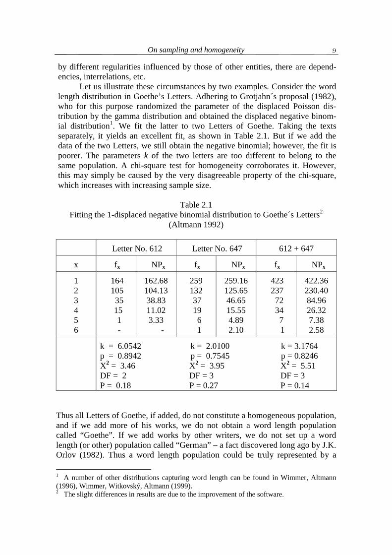
by different regularities influenced by those of other entities, there are depend-encies, interrelations, etc. Let us illustrate these circumstances by two examples. Consider the word length distribution in Goethe’s Letters. Adhering to Grotjahn´s proposal (1982), who for this purpose randomized the parameter of the displaced Poisson dis-tribution by the gamma distribution and obtained the displaced negative binom-ial distribution1. We fit the latter to two Letters of Goethe. Taking the texts separately, it yields an excellent fit, as shown in Table 2.1. But if we add the data of the two Letters, we still obtain the negative binomial; however, the fit is poorer. The parameters k of the two letters are too different to belong to the same population. A chi-square test for homogeneity corroborates it. However, this may simply be caused by the very disagreeable property of the chi-square, which increases with increasing sample size.

Table 2.1 Fitting the 1-displaced negative binomial distribution to Goethe´s Letters2

(Altmann 1992)

Letter No. 612

Letter No. 647

612 + 647

x

fx

NPx

fx

NPx

fx

NPx

1 2 3 4 5 6

164 105 35 15 1 -

162.68 104.13 38.83 11.02 3.33 -

259 132 37 19 6 1

259.16 125.65 46.65 15.55 4.89 2.10

423 237 72 34 7 1

422.36 230.40 84.96 26.32 7.38 2.58

k = 6.0542 k = 2.0100 k = 3.1764 p = 0.8942 p = 0.7545 p = 0.8246 X2 = 3.46 X2 = 3.95 X2 = 5.51 DF = 2 DF = 3 DF = 3 P = 0.18 P = 0.27 P = 0.14

Thus all Letters of Goethe, if added, do not constitute a homogeneous population, and if we add more of his works, we do not obtain a word length population called “Goethe”. If we add works by other writers, we do not set up a word length (or other) population called “German” – a fact discovered long ago by J.K. Orlov (1982). Thus a word length population could be truly represented by a 1 A number of other distributions capturing word length can be found in Wimmer, Altmann (1996), Wimmer, Witkovský, Altmann (1999). 2 The slight differences in results are due to the improvement of the software.

On sampling and homogeneity

10

weighted sum of probability mass functions. If one would consider also the part-of-speech character of words, one would obtain a sum of multidimensional prob-ability distributions. Needless to say, every science is simplification and approxi-mation, and we are not always aware or not forced to be aware of the basic non-homogeneity of our data.

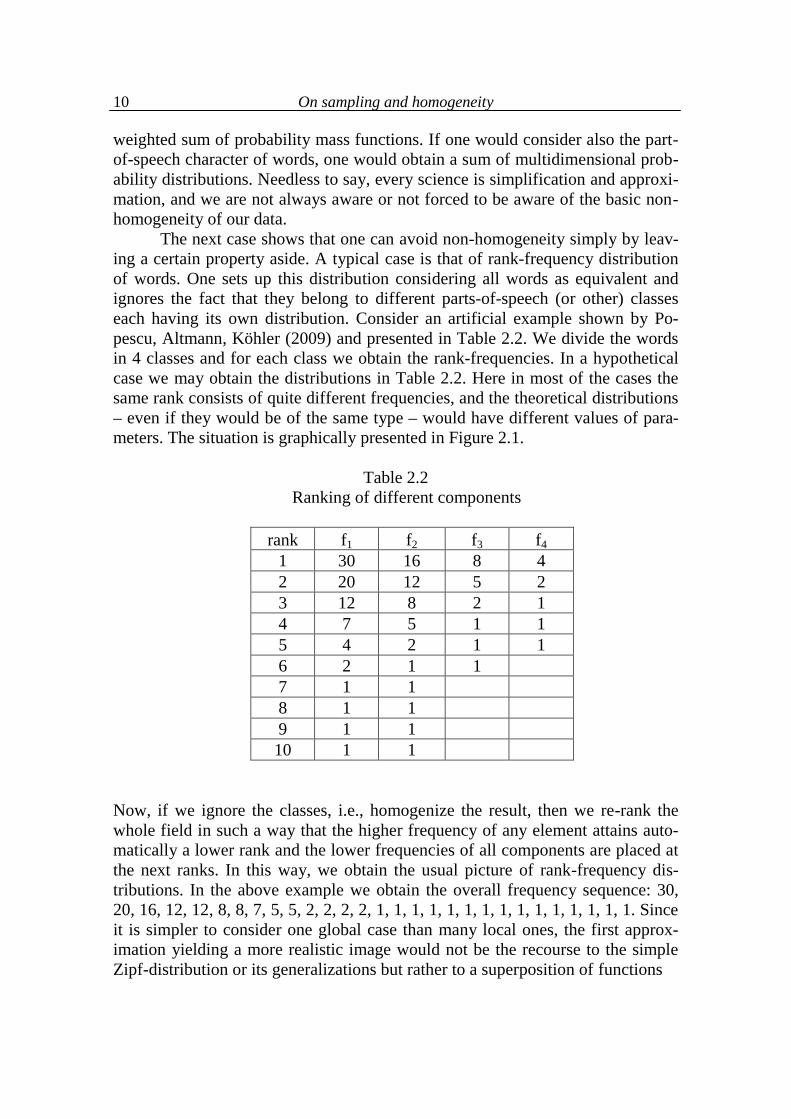
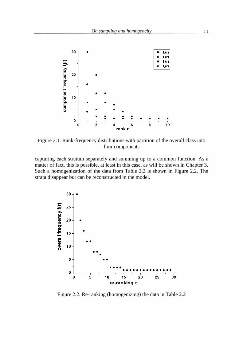
The next case shows that one can avoid non-homogeneity simply by leav-ing a certain property aside. A typical case is that of rank-frequency distribution of words. One sets up this distribution considering all words as equivalent and ignores the fact that they belong to different parts-of-speech (or other) classes each having its own distribution. Consider an artificial example shown by Po-pescu, Altmann, Köhler (2009) and presented in Table 2.2. We divide the words in 4 classes and for each class we obtain the rank-frequencies. In a hypothetical case we may obtain the distributions in Table 2.2. Here in most of the cases the same rank consists of quite different frequencies, and the theoretical distributions – even if they would be of the same type – would have different values of para-meters. The situation is graphically presented in Figure 2.1.

Table 2.2

Ranking of different components

rank f1 f2 f3 f4 1 30 16 8 4 2 20 12 5 2 3 12 8 2 1 4 7 5 1 1 5 4 2 1 1 6 2 1 1 7 1 1 8 1 1 9 1 1 10 1 1

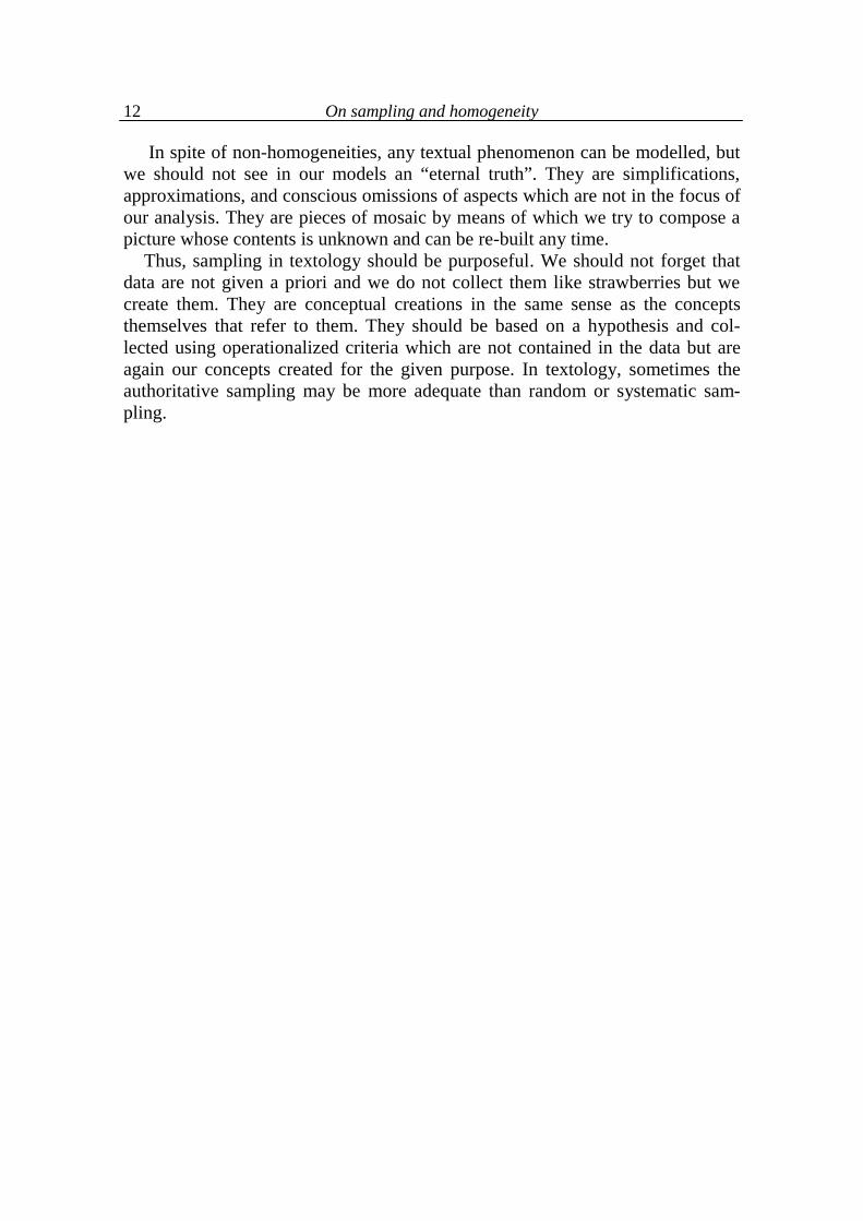
Now, if we ignore the classes, i.e., homogenize the result, then we re-rank the whole field in such a way that the higher frequency of any element attains auto-matically a lower rank and the lower frequencies of all components are placed at the next ranks. In this way, we obtain the usual picture of rank-frequency dis-tributions. In the above example we obtain the overall frequency sequence: 30, 20, 16, 12, 12, 8, 8, 7, 5, 5, 2, 2, 2, 2, 1, 1, 1, 1, 1, 1, 1, 1, 1, 1, 1, 1, 1, 1, 1. Since it is simpler to consider one global case than many local ones, the first approx-imation yielding a more realistic image would not be the recourse to the simple Zipf-distribution or its generalizations but rather to a superposition of functions

On sampling and homogeneity

11

Figure 2.1. Rank-frequency distributions with partition of the overall class into

four components capturing each stratum separately and summing up to a common function. As a matter of fact, this is possible, at least in this case, as will be shown in Chapter 3. Such a homogenization of the data from Table 2.2 is shown in Figure 2.2. The strata disappear but can be reconstructed in the model.

Figure 2.2. Re-ranking (homogenizing) the data in Table 2.2

On sampling and homogeneity

12

In spite of non-homogeneities, any textual phenomenon can be modelled, but we should not see in our models an “eternal truth”. They are simplifications, approximations, and conscious omissions of aspects which are not in the focus of our analysis. They are pieces of mosaic by means of which we try to compose a picture whose contents is unknown and can be re-built any time. Thus, sampling in textology should be purposeful. We should not forget that data are not given a priori and we do not collect them like strawberries but we create them. They are conceptual creations in the same sense as the concepts themselves that refer to them. They should be based on a hypothesis and col-lected using operationalized criteria which are not contained in the data but are again our concepts created for the given purpose. In textology, sometimes the authoritative sampling may be more adequate than random or systematic sam-pling.

3. A new view on Zipf´s law

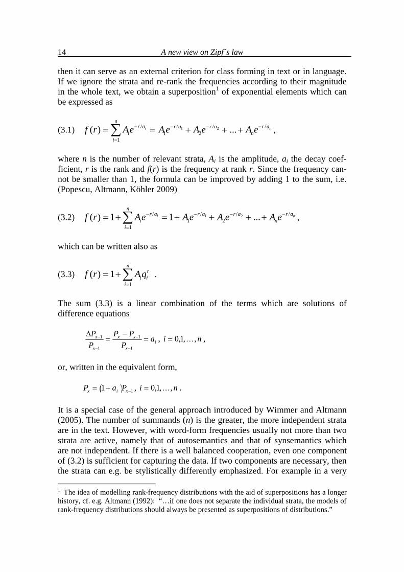
“Zipf´s law” is the general name by which the relation between the frequency fr and the rank r of any linguistic elements has been baptized. The number of formulas capturing this regularity is enormous (cf. http://www.nslij-genetics.org/ wli/zipf/ created by Wentian Li). Their exuberance was caused by two circum-stances: (1) The researchers tried to give it a better substantiation than Zipf and arrived automatically at different formulas. A part of the formulas are general-izations of the zeta distribution, another part are empirical modifications of Mandelbrot´s approach (which is itself a generalization of zeta) and a third part contains ad hoc trials based sometimes on analogies, proliferates in serendipity and is full of endeavours to obtain a better fit to data. Since the new mathemat-ical trials are made mostly by non-linguists, a failure in fitting a model to the given data is in turn corrected by a modification of the model. This technique enhances mathematical complexity. (2) However, in case of a failure, linguists concentrate on the first of the three steps of improvement: (a) check the data, (b) check the computation, (c) check the model. Since computations are performed today by means of a computer, textologists may concentrate only on data. But even textologists believe that data are given a priori. However, before one collects data, one must create them in the light of a hypothesis. A very remark-able example is, e.g., the modelling of the distribution of sentence length in texts having no punctuation e.g. Early High German official records. Here, “sentence length” is a concept which must be operationalized very exactly, otherwise one document = one sentence, then data are created from the text and, in the end, sentence length can be measured. In simple cases textologists operationalize a property and the measurement unit, but the non-homogeneity of the text − men-tioned in the previous chapter − is mostly not worth of attention. In a stage play there are as many parts as there are acts and as many strata as there are actors. If we mix up the shares of all actors in a unique data file, we sometimes obtain a not very regular function which significantly deviates from our previous models. And though the non-homogeneity is not so conspicuous in many texts, we have, nevertheless, several different intrinsic and extrinsic non-homogeneities which must be taken into account. They are due to (objective and subjective) conditions under which the text was created. In the case of word-form frequencies we have different parts of speech which can in turn be classified as autosemantics and synsemantics; there is the speech of the author and that of acting persons, the functions of words in the sentence, the restrictions of the genre, the technical domain within a genre, the style, etc. This all forms strata within which there is a leading element and a regularly decreasing share of the other elements. Here we conjecture further that within each stratum – if it is determined adequately – the decrease of frequencies of individual elements is very regular and has an exponential form or, considered in discrete steps, a form of a geometric sequence. If this conjecture is correct,

A new view on Zipf´s law

14

then it can serve as an external criterion for class forming in text or in language. If we ignore the strata and re-rank the frequencies according to their magnitude in the whole text, we obtain a superposition1 of exponential elements which can be expressed as

(3.1) 1 2/ // /1 2

1( ) ...i n

nr a r ar a r a

i ni

f r Ae A e A e A e

,

where n is the number of relevant strata, Ai is the amplitude, ai the decay coef-ficient, r is the rank and f(r) is the frequency at rank r. Since the frequency can-not be smaller than 1, the formula can be improved by adding 1 to the sum, i.e. (Popescu, Altmann, Köhler 2009)

(3.2) 1 2/ // /1 2

1( ) 1 1 ...i n

nr a r ar a r a

i ni

f r Ae Ae A e A e

,

which can be written also as

(3.3) 1

( ) 1n

ri i

if r Aq

.

The sum (3.3) is a linear combination of the terms which are solutions of difference equations

ix

xx

x

x aP

PPPP

1

1

1

1 , ni ,,1,0 ,

or, written in the equivalent form, 11 xix PaP , ni ,,1,0 . It is a special case of the general approach introduced by Wimmer and Altmann (2005). The number of summands (n) is the greater, the more independent strata are in the text. However, with word-form frequencies usually not more than two strata are active, namely that of autosemantics and that of synsemantics which are not independent. If there is a well balanced cooperation, even one component of (3.2) is sufficient for capturing the data. If two components are necessary, then the strata can e.g. be stylistically differently emphasized. For example in a very 1 The idea of modelling rank-frequency distributions with the aid of superpositions has a longer history, cf. e.g. Altmann (1992): “…if one does not separate the individual strata, the models of rank-frequency distributions should always be presented as superpositions of distributions.”

A new view on Zipf´s law

15

ornamental style the tail of the sequence may be considerably prolonged. In that case one can identify the following components: that with great Ai but small qi belonging to the quickly decreasing class, namely that of synsemantics, and that with small Ai but great qi being the slowly decreasing class of autosemantics. The necessity of a third or of more components gives a possibility of philological interpretations. Usually, one models the rank-frequency phenomenon using a discrete probability distribution. Zipf himself did not do it, he simply found a relation-ship, but was criticized for this reason (cf. e.g. Joos 1936), other researchers did it and were criticized, too, because rank is no random variable but a position in a sequence. This is probably the source of the myth of tautology of Zipf´s law. However, an ordered set is no myth and if the ordering can be expressed form-ally, there is neither an empirical nor a theoretical reason not to do it. Ranked frequencies simply represent a decreasing sequence of numbers, and the ranks are no measurable properties which could be ascribed to the words in the text by (operational) definition. If we do not expect more, there is no obstacle for seek-ing the form of this regularity. What more, the theoretical sequence (3.2) can even be replaced by a continuous function which would be a different approximation to the ordering regularity. As already mentioned, continuity and discreteness are properties of our concepts used especially in mathematical models, and not properties of reality. Needless to say, the model of the sequence can be normalized and in that case it yields a discrete probability distribution. The ranks play the role of an auxiliary random variable and no additional linguistic interpretation is necessary. The distributional approach has, however, some disadvantages. First, there are no homogeneous texts with infinite inventory, hence each theoretical distribution must be truncated at the right side. The majority of the models do not care for this circumstance. Second, the goodness-of-fit is estimated using the chi-square test whose weaknesses are well known. The major ones are: (i) the deviations in classes with great frequencies obtain a small weight but those with small fre-quencies great weights even if the small frequency can be caused by small sample size. That means, the goodness of fit can be decided on the basis of un-reliable classes. Pooling of frequency classes helps to moderate this flaw. (ii) The weighting of deviations is asymmetric. The same difference between theoretical and empirical frequency can obtain different weight: if e.g. O = 5 and E = 3, the difference is |O-E| = 2, and the component of the chi-square yields (5-3)2/3 = 1.33, but if O = 3 and E = 5, the component is (3-5)2/5 = 0.8. (iii) The usual chi-square test is a special case of the Cressie-Read statistics, in which the exponent need not be 2 but can be optimized. (iv) The chi-square is a sum of squared normal variables, i.e. based on normality of deviations. But in language there are no normal deviations; all of them are made in favour of the speaker/writer; they are always skewed. In language there are not even normal distributions. Such a state, i.e. normality, contradicts the nature and the development of language, as

A new view on Zipf´s law

16

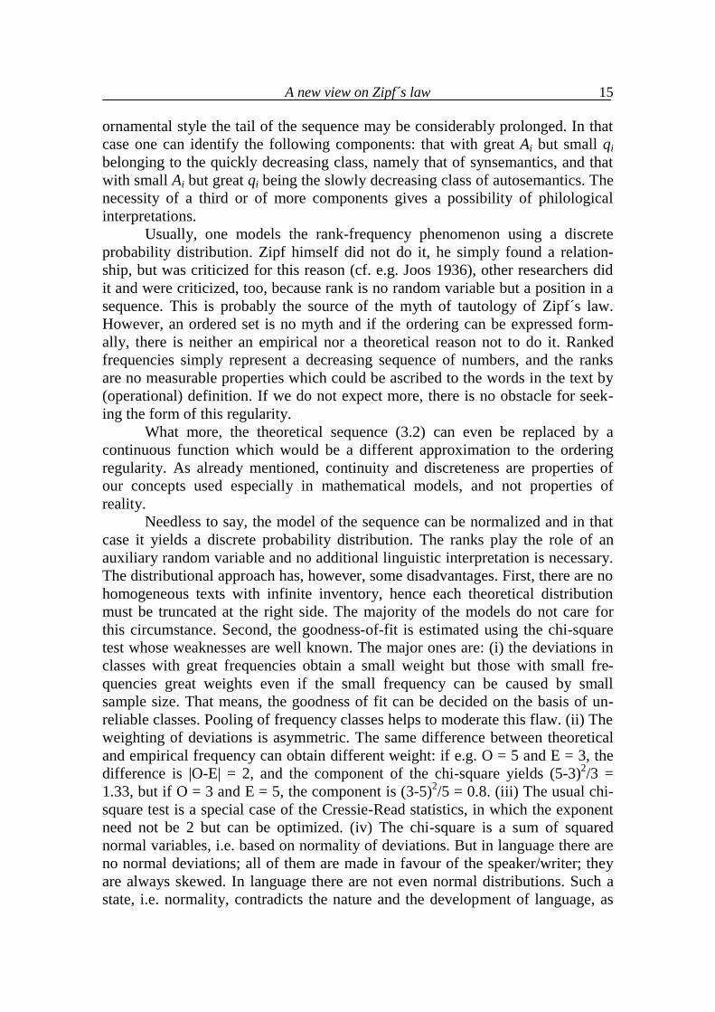
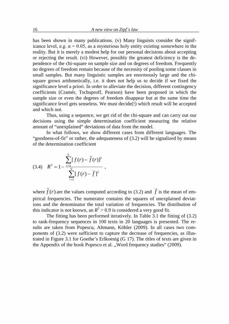
has been shown in many publications. (v) Many linguists consider the signif-icance level, e.g. α = 0.05, as a mysterious holy entity existing somewhere in the reality. But it is merely a modest help for our personal decisions about accepting or rejecting the result. (vi) However, possibly the greatest deficiency is the de-pendence of the chi-square on sample size and on degrees of freedom. Frequently no degrees of freedom remain because of the necessity of pooling some classes in small samples. But many linguistic samples are enormously large and the chi-square grows arithmetically, i.e. it does not help us to decide if we fixed the significance level a priori. In order to alleviate the decision, different contingency coefficients (Cramér, Tschuproff, Pearson) have been proposed in which the sample size or even the degrees of freedom disappear but at the same time the significance level gets senseless. We must decide(!) which result will be accepted and which not. Thus, using a sequence, we get rid of the chi-square and can carry out our decisions using the simple determination coefficient measuring the relative amount of “unexplained” deviations of data from the model. In what follows, we show different cases from different languages. The “goodness-of-fit” or rather, the adequateness of (3.2) will be signalized by means of the determination coefficient

(3.4)

2

2 1

2

1

ˆ[ ( ) ( )]1

[ ( ) ]

V

rV

r

f r f rR

f r f

,

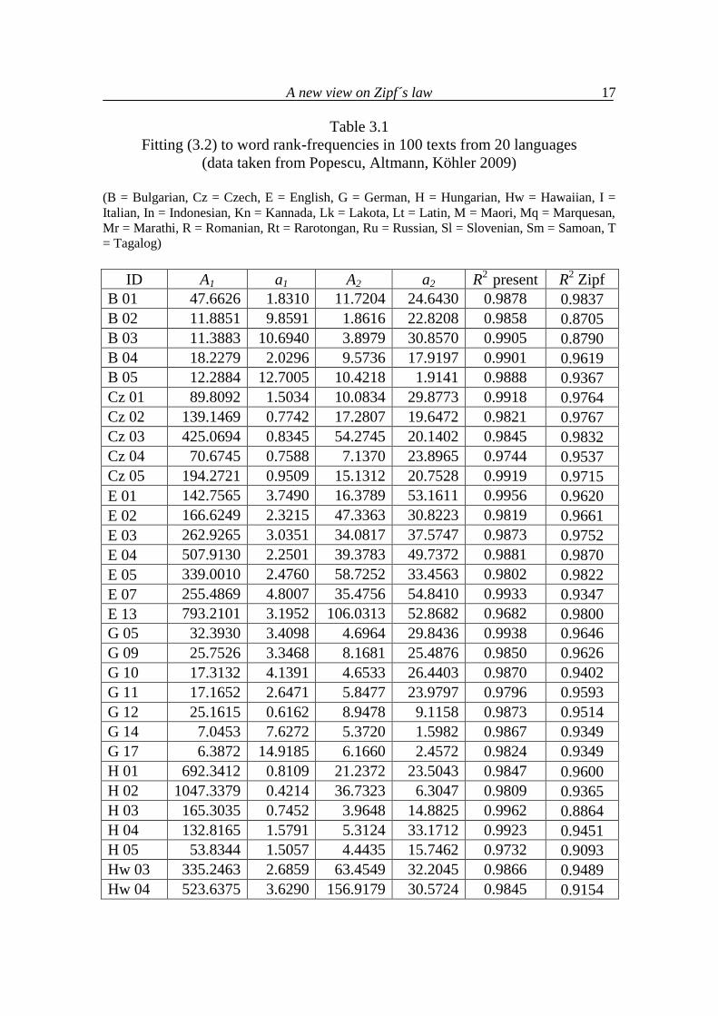
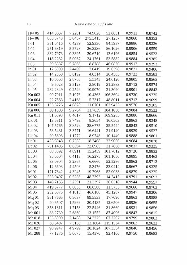
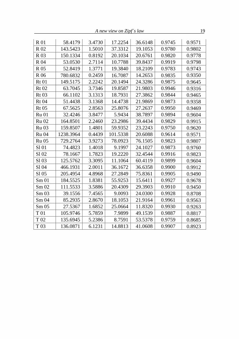
where ˆ ( )f r are the values computed according to (3.2) and f is the mean of em-pirical frequencies. The numerator contains the squares of unexplained deviat-ions and the denominator the total variation of frequencies. The distribution of this indicator is not known, an R2 > 0.9 is considered a very good fit. The fitting has been performed iteratively. In Table 3.1 the fitting of (3.2) to rank-frequency sequences in 100 texts in 20 languages is presented. The re-sults are taken from Popescu, Altmann, Köhler (2009). In all cases two com-ponents of (3.2) were sufficient to capture the decrease of frequencies, as illus-trated in Figure 3.1 for Goethe’s Erlkoenig (G 17). The titles of texts are given in the Appendix of the book Popescu et al. „Word frequency studies“ (2009).

A new view on Zipf´s law

17

Table 3.1 Fitting (3.2) to word rank-frequencies in 100 texts from 20 languages

(data taken from Popescu, Altmann, Köhler 2009)

(B = Bulgarian, Cz = Czech, E = English, G = German, H = Hungarian, Hw = Hawaiian, I = Italian, In = Indonesian, Kn = Kannada, Lk = Lakota, Lt = Latin, M = Maori, Mq = Marquesan, Mr = Marathi, R = Romanian, Rt = Rarotongan, Ru = Russian, Sl = Slovenian, Sm = Samoan, T = Tagalog)

ID A1 a1 A2 a2 R2 present R2 Zipf

B 01 47.6626 1.8310 11.7204 24.6430 0.9878 0.9837 B 02 11.8851 9.8591 1.8616 22.8208 0.9858 0.8705 B 03 11.3883 10.6940 3.8979 30.8570 0.9905 0.8790 B 04 18.2279 2.0296 9.5736 17.9197 0.9901 0.9619 B 05 12.2884 12.7005 10.4218 1.9141 0.9888 0.9367 Cz 01 89.8092 1.5034 10.0834 29.8773 0.9918 0.9764 Cz 02 139.1469 0.7742 17.2807 19.6472 0.9821 0.9767 Cz 03 425.0694 0.8345 54.2745 20.1402 0.9845 0.9832 Cz 04 70.6745 0.7588 7.1370 23.8965 0.9744 0.9537 Cz 05 194.2721 0.9509 15.1312 20.7528 0.9919 0.9715 E 01 142.7565 3.7490 16.3789 53.1611 0.9956 0.9620 E 02 166.6249 2.3215 47.3363 30.8223 0.9819 0.9661 E 03 262.9265 3.0351 34.0817 37.5747 0.9873 0.9752 E 04 507.9130 2.2501 39.3783 49.7372 0.9881 0.9870 E 05 339.0010 2.4760 58.7252 33.4563 0.9802 0.9822 E 07 255.4869 4.8007 35.4756 54.8410 0.9933 0.9347 E 13 793.2101 3.1952 106.0313 52.8682 0.9682 0.9800 G 05 32.3930 3.4098 4.6964 29.8436 0.9938 0.9646 G 09 25.7526 3.3468 8.1681 25.4876 0.9850 0.9626 G 10 17.3132 4.1391 4.6533 26.4403 0.9870 0.9402 G 11 17.1652 2.6471 5.8477 23.9797 0.9796 0.9593 G 12 25.1615 0.6162 8.9478 9.1158 0.9873 0.9514 G 14 7.0453 7.6272 5.3720 1.5982 0.9867 0.9349 G 17 6.3872 14.9185 6.1660 2.4572 0.9824 0.9349 H 01 692.3412 0.8109 21.2372 23.5043 0.9847 0.9600 H 02 1047.3379 0.4214 36.7323 6.3047 0.9809 0.9365 H 03 165.3035 0.7452 3.9648 14.8825 0.9962 0.8864 H 04 132.8165 1.5791 5.3124 33.1712 0.9923 0.9451 H 05 53.8344 1.5057 4.4435 15.7462 0.9732 0.9093 Hw 03 335.2463 2.6859 63.4549 32.2045 0.9866 0.9489 Hw 04 523.6375 3.6290 156.9179 30.5724 0.9845 0.9154

A new view on Zipf´s law

18

Hw 05 414.8637 7.2201 74.9028 52.8651 0.9911 0.8742 Hw 06 865.3743 3.0457 275.3415 27.1237 0.9868 0.9352 I 01 381.6416 6.4239 52.9336 84.5937 0.9886 0.9336 I 02 251.6319 5.5728 26.3236 86.1026 0.9906 0.9559 I 03 832.7973 0.3395 20.6710 13.6196 0.9854 0.9523 I 04 118.2232 5.0067 24.1761 53.5882 0.9884 0.9385 I 05 39.6387 5.7866 8.8788 46.0830 0.9912 0.9293 In 01 12.5099 2.4489 7.0419 19.6398 0.9821 0.9486 In 02 14.2350 3.6192 4.8314 26.4565 0.9722 0.9583 In 03 10.0663 2.8763 5.5343 24.6120 0.9805 0.9565 In 04 9.5023 2.5123 3.8019 31.2883 0.9712 0.9574 In 05 232.2849 0.2549 10.9070 21.3090 0.9901 0.8843 Kn 003 90.7911 2.1976 10.4363 106.3604 0.9730 0.9775 Kn 004 22.7563 2.4168 5.7317 48.8011 0.9713 0.9699 Kn 005 133.3226 4.0828 11.0701 162.9435 0.9576 0.9105 Kn 006 60.1808 9.2704 11.7639 184.1050 0.9884 0.9522 Kn 011 51.6393 8.4017 9.1712 169.9285 0.9886 0.9666 Lk 01 13.5811 3.7493 8.3654 16.0503 0.9863 0.9348 Lk 02 107.5765 3.8529 28.6775 25.5444 0.9843 0.9510 Lk 03 58.5481 3.3771 16.6441 21.9140 0.9929 0.9527 Lk 04 20.5803 1.1772 8.9748 10.1449 0.9888 0.9801 Lt 01 423.6948 0.7583 18.3468 32.9066 0.9684 0.9078 Lt 02 751.1495 0.6394 32.6985 31.7868 0.9837 0.9335 Lt 03 88.3092 4.8911 15.2459 101.7612 0.9720 0.9832 Lt 04 95.6604 6.4113 16.2275 101.1050 0.9895 0.9463 Lt 05 33.0904 3.2367 6.6660 52.5286 0.9862 0.9713 Lt 06 12.6603 4.4508 5.3476 33.0414 0.9667 0.9325 M 01 171.7642 4.3245 19.7968 52.0033 0.9879 0.9225 M 02 533.0407 0.5286 48.7393 14.2415 0.9791 0.9693 M 03 146.7155 3.2391 21.3397 36.0318 0.9944 0.9557 M 04 419.3777 0.6036 60.6588 11.5735 0.9666 0.9763 M 05 252.6075 4.1815 46.6180 45.1287 0.9947 0.9306 Mq 01 951.7665 0.5637 89.5533 17.7090 0.9863 0.9588 Mq 02 40.6507 1.5969 20.4135 12.6506 0.9926 0.9655 Mq 03 353.1811 1.7158 22.5446 31.8669 0.9931 0.9856 Mr 001 88.2739 2.6860 13.1552 87.4096 0.9842 0.9815 Mr 018 155.3090 2.1488 24.7275 67.2207 0.9799 0.9863 Mr 026 68.5407 7.3158 13.1804 115.1534 0.9863 0.9633 Mr 027 90.9947 4.9799 20.1624 107.3354 0.9846 0.9456 Mr 288 77.1276 5.0675 15.4370 92.4166 0.9750 0.9683

A new view on Zipf´s law

19

R 01 58.4179 3.4730 17.2254 36.6148 0.9745 0.9571 R 02 143.5423 1.5010 37.3312 19.1053 0.9780 0.9802 R 03 150.1334 0.8192 20.1034 20.6761 0.9820 0.9778 R 04 53.0530 2.7114 10.7788 39.8437 0.9919 0.9798 R 05 52.8419 1.3771 19.3840 18.2109 0.9783 0.9743 R 06 780.6832 0.2459 16.7087 14.2653 0.9835 0.9350 Rt 01 149.5175 2.2242 20.1494 24.3286 0.9875 0.9645 Rt 02 63.7045 3.7346 19.8587 21.9803 0.9946 0.9316 Rt 03 66.1102 3.1313 18.7931 27.3862 0.9844 0.9465 Rt 04 51.4438 3.1368 14.4738 21.9869 0.9873 0.9358 Rt 05 67.5625 2.8563 25.8076 27.2637 0.9950 0.9469 Ru 01 32.4246 3.8477 5.9434 38.7897 0.9894 0.9604 Ru 02 164.8501 2.2460 23.2986 39.4434 0.9829 0.9915 Ru 03 159.8507 1.4801 59.9352 23.2243 0.9750 0.9620 Ru 04 1238.3964 0.4439 101.5338 20.6088 0.9614 0.9571 Ru 05 729.2764 3.9273 78.0923 76.1505 0.9823 0.9807 Sl 01 74.4823 1.4018 9.1997 24.1027 0.9873 0.9760 Sl 02 78.1667 1.7823 19.2220 32.4544 0.9916 0.9823 Sl 03 125.5762 3.3095 11.1064 60.4119 0.9899 0.9604 Sl 04 466.1931 2.0011 36.1672 36.6358 0.9900 0.9912 Sl 05 205.4954 4.8968 27.2849 75.8361 0.9905 0.9490 Sm 01 184.5525 1.8381 55.9253 15.6411 0.9927 0.9678 Sm 02 111.5533 3.5886 20.4309 29.3903 0.9910 0.9450 Sm 03 39.1556 7.4565 9.0093 24.0300 0.9928 0.8708 Sm 04 85.2935 2.8670 18.1053 21.9164 0.9961 0.9563 Sm 05 27.5367 1.6852 25.0664 11.8320 0.9930 0.9263 T 01 105.9746 5.7859 7.9899 49.1539 0.9887 0.8817 T 02 135.6945 5.2386 8.7591 53.5378 0.9759 0.8685 T 03 136.0871 6.1231 14.8813 41.0608 0.9907 0.8923

A new view on Zipf´s law

20

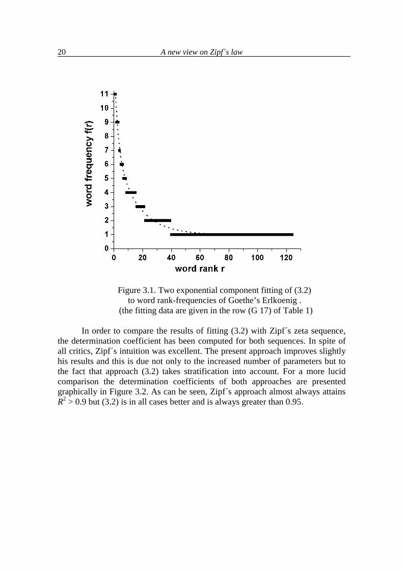
Figure 3.1. Two exponential component fitting of (3.2)

to word rank-frequencies of Goethe’s Erlkoenig . (the fitting data are given in the row (G 17) of Table 1)

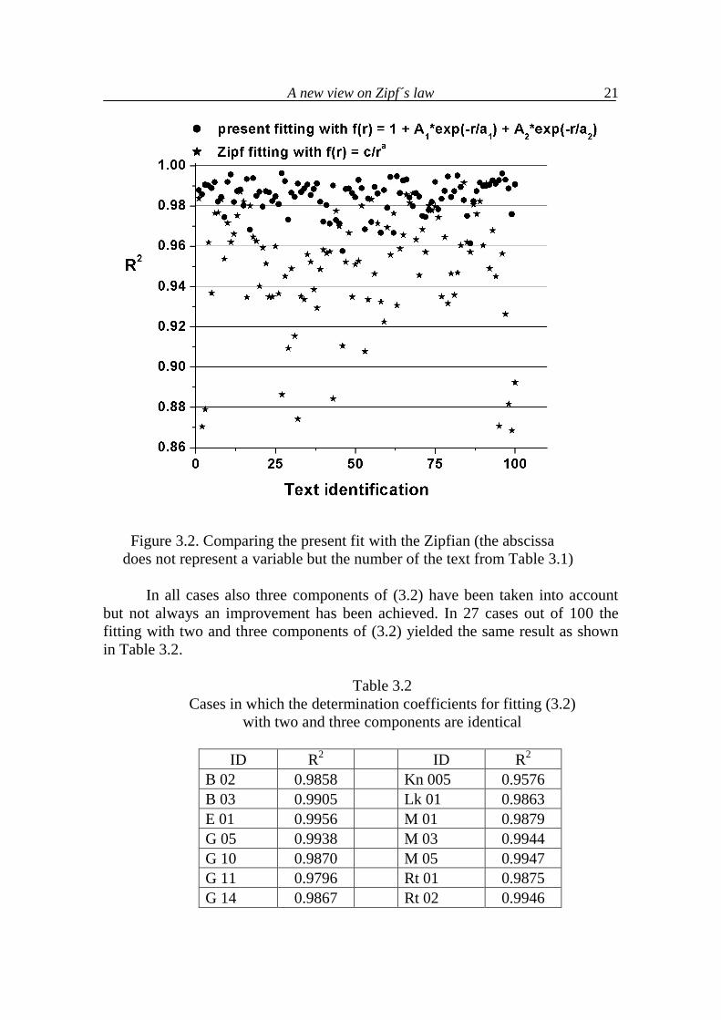
In order to compare the results of fitting (3.2) with Zipf´s zeta sequence, the determination coefficient has been computed for both sequences. In spite of all critics, Zipf´s intuition was excellent. The present approach improves slightly his results and this is due not only to the increased number of parameters but to the fact that approach (3.2) takes stratification into account. For a more lucid comparison the determination coefficients of both approaches are presented graphically in Figure 3.2. As can be seen, Zipf´s approach almost always attains R2 > 0.9 but (3.2) is in all cases better and is always greater than 0.95.

A new view on Zipf´s law

21

Figure 3.2. Comparing the present fit with the Zipfian (the abscissa does not represent a variable but the number of the text from Table 3.1)

In all cases also three components of (3.2) have been taken into account but not always an improvement has been achieved. In 27 cases out of 100 the fitting with two and three components of (3.2) yielded the same result as shown in Table 3.2.

Table 3.2

Cases in which the determination coefficients for fitting (3.2) with two and three components are identical

ID R2 ID R2

B 02 0.9858 Kn 005 0.9576 B 03 0.9905 Lk 01 0.9863 E 01 0.9956 M 01 0.9879 G 05 0.9938 M 03 0.9944 G 10 0.9870 M 05 0.9947 G 11 0.9796 Rt 01 0.9875 G 14 0.9867 Rt 02 0.9946

A new view on Zipf´s law

22

G 17 0.9824 Ru 01 0.9894 H 05 0.9732 Sl 03 0.9899 Hw 03 0.9866 Sm 03 0.9928 In 01 0.9821 Sm 04 0.9961 In 03 0.9805 T 01 0.9887 In 04 0.9712 T 02 0.9759 In 05 0.9901

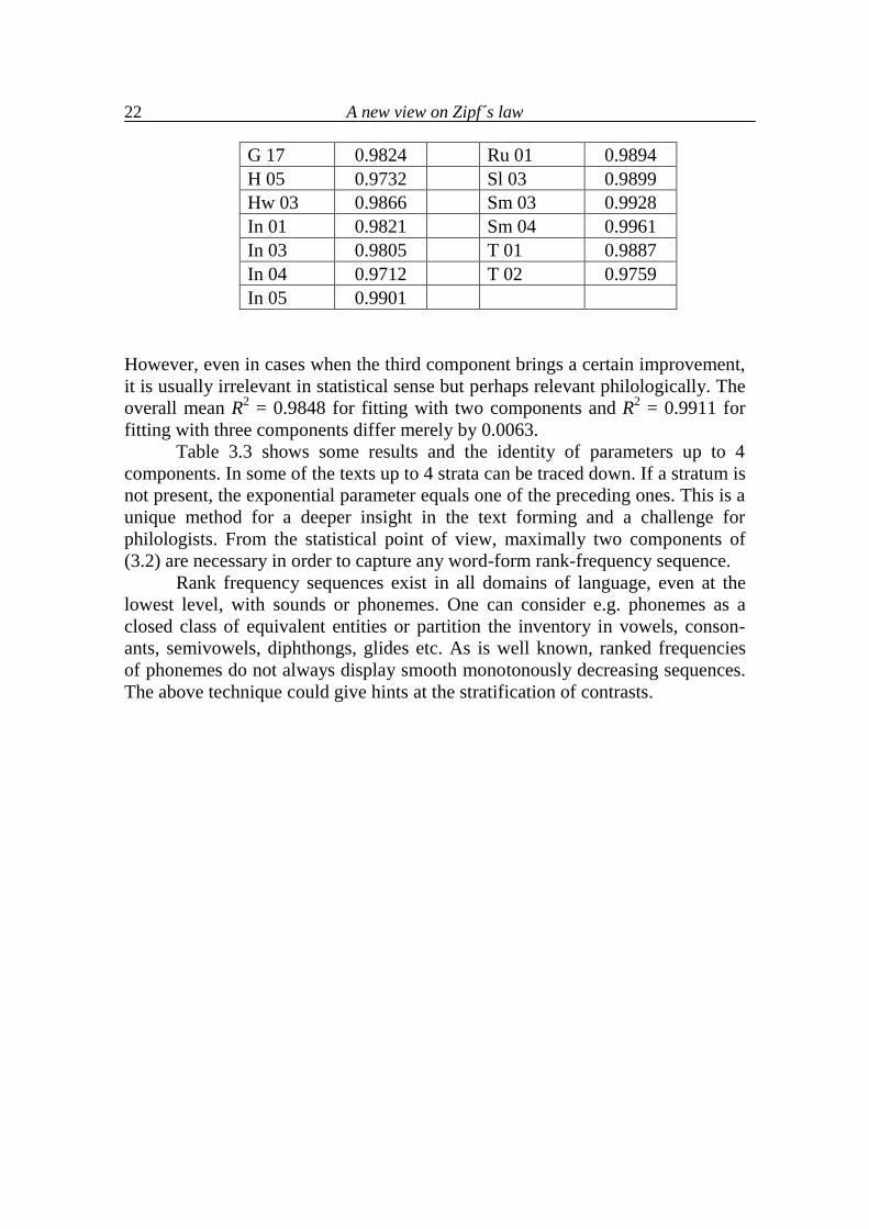
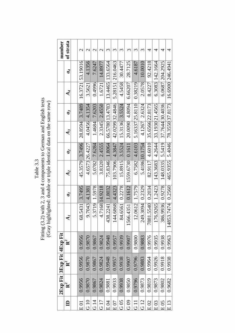
However, even in cases when the third component brings a certain improvement, it is usually irrelevant in statistical sense but perhaps relevant philologically. The overall mean R2 = 0.9848 for fitting with two components and R2 = 0.9911 for fitting with three components differ merely by 0.0063. Table 3.3 shows some results and the identity of parameters up to 4 components. In some of the texts up to 4 strata can be traced down. If a stratum is not present, the exponential parameter equals one of the preceding ones. This is a unique method for a deeper insight in the text forming and a challenge for philologists. From the statistical point of view, maximally two components of (3.2) are necessary in order to capture any word-form rank-frequency sequence. Rank frequency sequences exist in all domains of language, even at the lowest level, with sounds or phonemes. One can consider e.g. phonemes as a closed class of equivalent entities or partition the inventory in vowels, conson-ants, semivowels, diphthongs, glides etc. As is well known, ranked frequencies of phonemes do not always display smooth monotonously decreasing sequences. The above technique could give hints at the stratification of contrasts.

Tabl

e 3.

3 Fi

tting

(3.2

) with

2, 3

and

4 c

ompo

nent

s to

Ger

man

and

Eng

lish

text

s (G

ray

high

light

ed: d

oubl

e or

trip

le id

entic

al d

ata

on th

e sa

me

row

)

2Exp

Fit

3Exp

Fit

4Exp

Fit

ID

R2

R2

R2

A 1

a 1

A 2

a 2

A 3

a 3

A 4

a 4

num

ber

of

stra

ta

E 01

0.

9956

0.

9956

0.

9956

68

.543

1 3.

7495

45

.357

9 3.

7496

28

.859

4 3.

7489

16

.372

1 53

.190

16

2 G

10

0.98

70

0.98

70

0.98

70

9.70

43

4.13

81

4.65

73 2

6.42

27

4.04

56

4.13

54

3.56

21

4.13

56

2 G

14

0.98

67

0.98

67

0.98

67

5.37

19

1.59

78

5.07

82

7.62

84

1.46

84

7.62

03

0.49

96

7.62

47

2 G

17

0.98

24

0.98

24

0.98

24

4.71

68 1

4.92

18

3.83

20

2.45

55

2.33

45

2.45

50

1.67

21

14.8

977

2 E

04

0.98

81

0.99

48

0.99

48

438.

2241

1.

8032

75

.834

6 1.

8064

66

.578

0 13

.478

3 13

.446

5 13

3.65

64

3 E

07

0.99

33

0.99

57

0.99

57

144.

6868

4.

4323

10

3.79

06

4.38

47

42.0

299

32.4

846

5.28

151

216.

0463

3

G 0

5 0.

9938

0.

9938

0.

9939

84

.656

1 0.

2278

15

.891

5 3.

5524

15

.313

6 3.

5524

4.

5458

30

.447

7 3

G 0

9 0.

9850

0.

9907

0.

9907

156

6.43

51

0.16

12 1

559.

6730

0.

1611

20

.009

0 4.

8094

6.

6620

7 28

.712

5 3

G 1

1 0.

9796

0.

9796

0.

9800

12

.061

2 1.

7579

6.

7582

4.

6103

5.

1633

7 25

.811

0 0.

3821

9 4.

6187

3

G 1

2 0.

9873

0.

9883

0.

9883

24

9.30

94

0.23

29

5.41

86 1

0.17

54

4.12

67

2.63

24

2.05

78

10.0

010

3 E

02

0.98

19

0.99

64

0.99

76

7881

.554

0 0.

2034

82

.911

7 4.

6010

35

.656

6 22

.817

3 8.

4227

92

.421

8 4

E 03

0.

9873

0.

9926

0.

9935

17

6.92

65

1.24

23

143.

3683

4.

2644

33

.193

0 21

.456

5 6.

3083

142

.166

4 4

E 05

0.

9802

0.

9918

0.

9938

38

6.99

36

0.92

78

148.

0335

5.

5419

37

.764

4 30

.403

6 6.

0687

204

.292

5 4

E 13

0.

9682

0.

9938

0.

9963

14

853.

7474

0.

2560

46

5.93

55

5.40

46

78.3

550

37.8

173

16.6

900

246.

4941

4

4. The h-point

The h-point can be defined as that point at which the straight line between two (usually) neighbouring ranked frequencies intersects the y = x line. Solving two simultaneous equations we obtain the definition

(4.1)

, ( )( ) ( )

, ( )( ) ( )

j i

j i

r if there is an r f rf i r f j rh

if there is no r f rr r f i f j

.

In other words, the h-point is that point at which r = f(r). If there is no such point, one takes, if possible, two neighbouring f(i) and f(j) such that f(i) > ri and f(j) < rj. Mostly ri + 1 = rj. As an example consider the last column in Table 2.2 in Chapter 2 where we have r 1, 2, 3, 4, 5 f(r) 4, 2, 1, 1, 1 Here, evidently h = 2 because the frequency at rank 2 is 2. However, the overall sequence of frequencies in Chapter 2 is r 1, 2, 3, 4, 5, 6, 7 , 8,9,10, 11, 12, 13, 14,15, 16, 17,18,19,20, 21,22,23, 24,25, 26,27,28,29 f(r) 30,20,16,12,12,8,8,7,5, 5, 2, 2, 2, 2, 1, 1, 1, 1, 1, 1, 1, 1, 1, 1, 1, 1, 1, 1, 1. Here, there is no r = f(r), but r = 7, f(7) = 8 and r = 8, f(8) = 7 fulfil the above condition. Inserting these values in the second part of (4.1) we obtain

(7)8 (8)7 8(8) 7(7) 7.5

8 7 (7) (8) 8 7 8 7f fh

f f

,

here the average of two ranks, but it need not be always the case. Other comput-ing possibilities have been presented in the extensive literature. The h-point has been created in scientometrics by Hirsch (2005) and discussed there and in documentation mathematically (cf. e.g. Bornmann, Daniel 2005; Egghe 2007a,b, 2008; Egghe, Rao 2008; Egghe, Rousseau 2006; Rousseau 2007; Rousseau, Liu 2008); in linguistics it appeared for the first time in Popescu (2007). This remarkable point is an attractive fixed-point having different uses in textology (cf. http://en.wikipedia.org/wiki/ Fixed_point_%28mathematics%29). In other applications, e.g. parts of speech, where the inventory is too small, neither of the two conditions may be fulfilled. For example in the se-quence

The h-point

25

r 1, 2, 3, 4, 5, 6 f(r) 100, 80, 60,50,40,30

where all f(r) > r. The problem can be solved in different ways but we prefer the transformation

(4.2) f*(r) = f(r) – f(V) + 1, for all r,

where V is the greatest rank, warranting that f*(V) = 1 < V. For the above se-quence we obtain 100 - 30 + 1 = 71 etc. hence r 1, 2, 3, 4, 5, 6 f*(r) 71,51,31,21,11,1 where r = 5 and 6 fulfil the above condition and one obtains h = 5.55. The h-point seems to be an important indicator in rank-frequency phen-omena. As is well known, every text consists of autosemantics which bring up the theme and the concomitant information, and of synsemantics which care for correct relations between autosemantics and sentences, furnish references and modify the autosemantics. The number of synsemantics is always greater than that of autosemantics, and usually they occupy the first ranks. The h-point forms a fuzzy threshold between these two kinds of words. Of course, some syn-semantics seldom occur – depending on style – and occupy some higher ranks. On the other hand, some autosemantics may occur more frequently than f(h) and their occurrence in the pre-h domain signalizes their association to the theme of the text. In fiction one often finds proper names in the pre-h domain but in scientific and technical texts these words are always thematic words. The more autosemantics are in this domain and the more frequent they are, the greater the thematic concentration of the text. Popescu and Altmann (2007a) proposed the indicator of thematic concentration in form

(4.3) 1

( ) ( )2( 1) (1)

h

r

h r f rTCh h f

,

where r´ are the ranks of autosemantics occupying ranks smaller than h. Here the difference between the pertinent ranks is weighted by the given frequency, and the sum of the differences is divided by the possible maximum. Since TC is a very small number, one usually multiplies it by a constant, e.g. 1000 and obtains a thematic concentration unit tcu = 1000(TC). A survey of tcu-values can be

The h-point

26

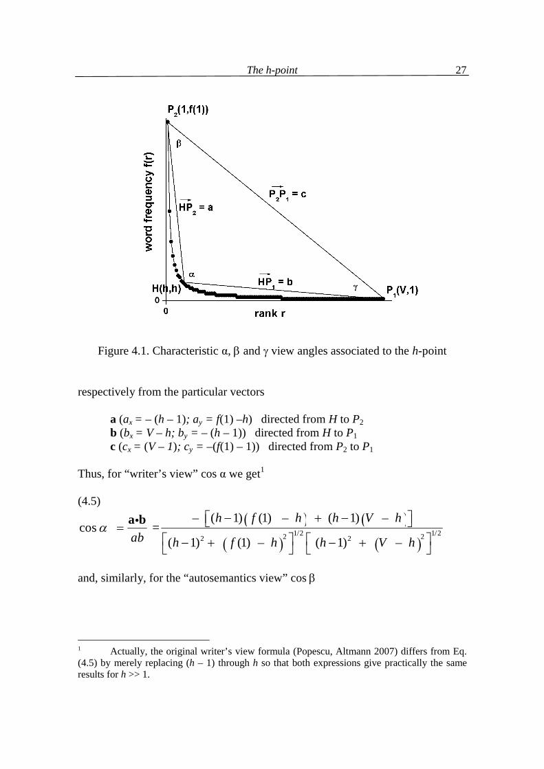
found in the book Popescu et al. (2009) and a recent extension of the TC concept in Tuzzi, Popescu, Altmann (2009). Some further useful indicators and functions associated to the h-point are the crowding of autosemantics, autosemantic pace filling, autosemantic compact-ness and writer´s view (cf. Popescu 2007; Popescu, Altmann 2006a,b, 2007; Popescu, Best, Altmann 2007; Popescu et al. 2008; Mačutek, Popescu, Altmann 2007) all of which can be used for stylistic analyses and can provide us with a deeper insight in the structure of texts. Here we shall consider the angles of the rank-frequency distribution and present bi- and triangular text and language classifications. Three relevant angular fields imply the h-point, as shown in Figure 1, namely the “writer’s view” angle α between the distribution end (P1) and top (P2) as seen from the h-point (H), baptized in this way because one can imagine the writer “sitting” at this point and controlling the equilibrium between auto-semantics and synsemantics (cf. Popescu, Altmann 2007); the view angle of the autosemantic arch span (P1H) as seen from the top (P2), and the view angle of the synsemantic arch span (P2H) as seen from the end (P1). One can imagine these angles as word-frequency self-regulation means. They are unconscious but they care for shaping the frequencies. Texts can attain some extreme points, but the variation is very restricted. Let us further derive the expressions of the natural cosines of these angles (“natural” means in radians) starting from the general expression of the scalar (dot) product of two vectors a (ax, ay) and b (bx, by), namely

(4.4) 1/2 1/22 2 2 2

cos

x x y y

x y x y

a b a bab a a b b

a b

and from the particular coordinates of the corners of the distribution characteristic triangle P1P2H given by

P1 (V, 1) P2 (1, f(1))

H (h, h)

The h-point

27

Figure 4.1. Characteristic α, and view angles associated to the h-point

respectively from the particular vectors a (ax = – (h – 1); ay = f(1) –h) directed from H to P2 b (bx = V – h; by = – (h – 1)) directed from H to P1 c (cx = (V – 1); cy = –(f(1) – 1)) directed from P2 to P1 Thus, for “writer’s view” cos α we get1 (4.5)

1/2 1/22 22 2

– ( 1) (1) – ( 1) – cos =  

( 1) (1) – ( 1) –

h f h h V hab h f h h V h

a b

and, similarly, for the “autosemantics view” cos

1 Actually, the original writer’s view formula (Popescu, Altmann 2007) differs from Eq. (4.5) by merely replacing (h – 1) through h so that both expressions give practically the same results for h >> 1.

The h-point

28

(4.6)

1/2 1/222 2 2

( 1)( 1) ( (1) 1) (1) – –cos ( 1) + (1) – ( 1) ( (1) 1)

h V f f hb

ac h f h V f

a c

and for the “synsemantics view” cos

(4.7)

1/21/2 22 2 2

( 1) – ( 1)( (1) 1)cos

( 1) ( (1) 1) ( 1) –

V V h h fbc V f h V h

b c

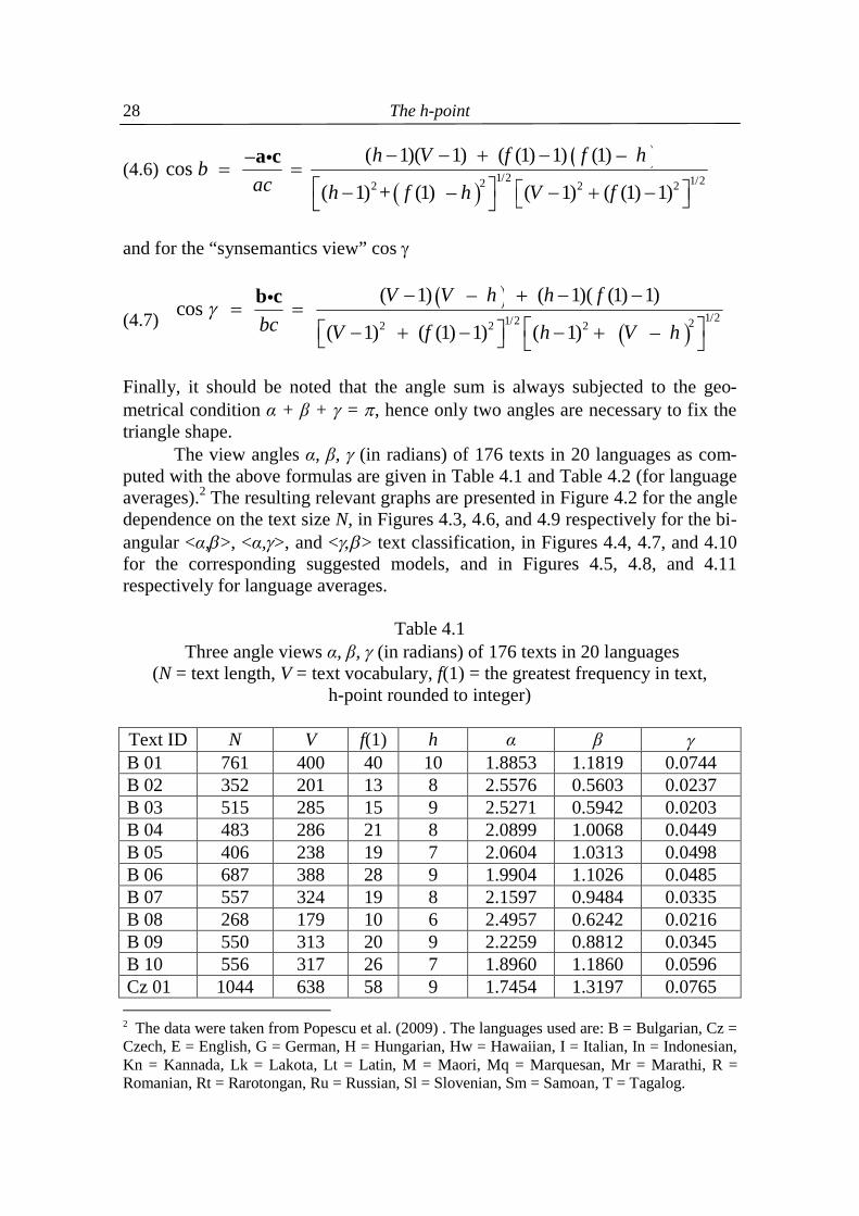
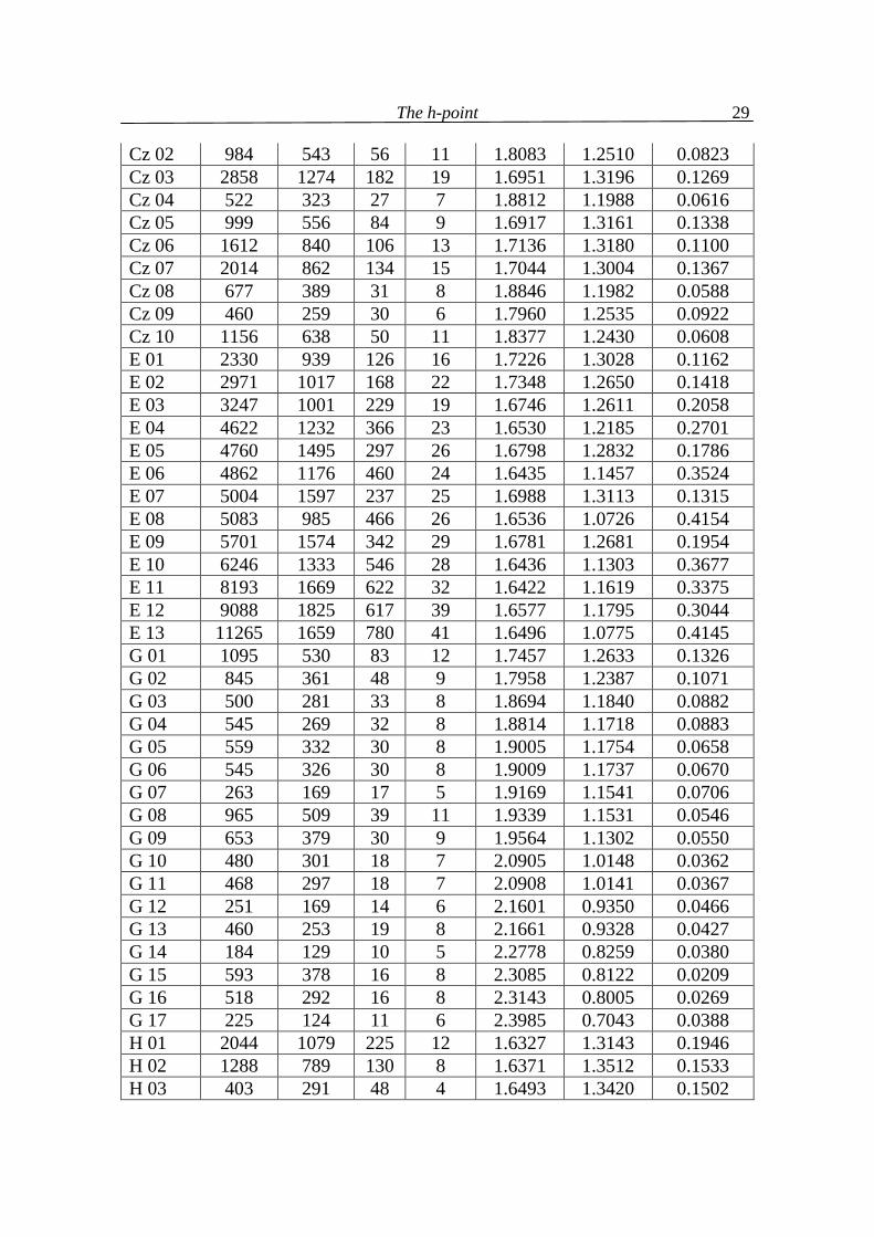
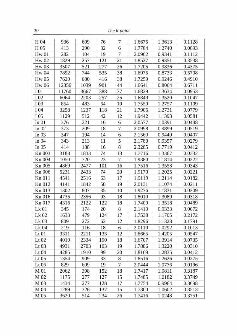
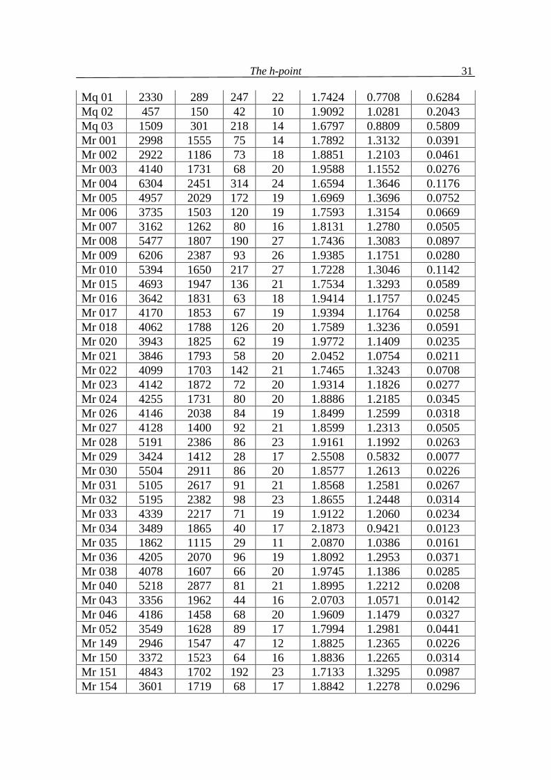
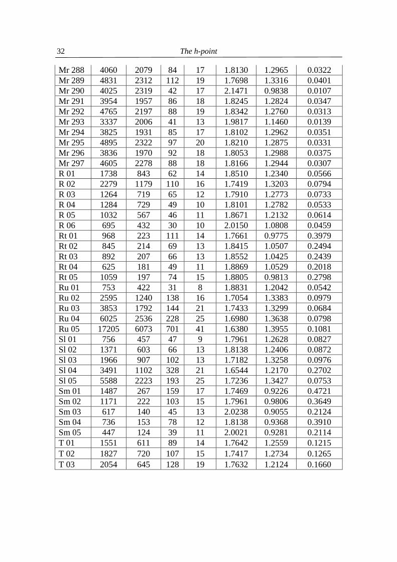
Finally, it should be noted that the angle sum is always subjected to the geo-metrical condition α + β + = , hence only two angles are necessary to fix the triangle shape. The view angles α, β, (in radians) of 176 texts in 20 languages as com-puted with the above formulas are given in Table 4.1 and Table 4.2 (for language averages).2 The resulting relevant graphs are presented in Figure 4.2 for the angle dependence on the text size N, in Figures 4.3, 4.6, and 4.9 respectively for the bi-angular <α,>, <α,>, and <> text classification, in Figures 4.4, 4.7, and 4.10 for the corresponding suggested models, and in Figures 4.5, 4.8, and 4.11 respectively for language averages.

Table 4.1 Three angle views α, β, (in radians) of 176 texts in 20 languages

(N = text length, V = text vocabulary, f(1) = the greatest frequency in text, h-point rounded to integer)

Text ID N V f(1) h α β B 01 761 400 40 10 1.8853 1.1819 0.0744 B 02 352 201 13 8 2.5576 0.5603 0.0237 B 03 515 285 15 9 2.5271 0.5942 0.0203 B 04 483 286 21 8 2.0899 1.0068 0.0449 B 05 406 238 19 7 2.0604 1.0313 0.0498 B 06 687 388 28 9 1.9904 1.1026 0.0485 B 07 557 324 19 8 2.1597 0.9484 0.0335 B 08 268 179 10 6 2.4957 0.6242 0.0216 B 09 550 313 20 9 2.2259 0.8812 0.0345 B 10 556 317 26 7 1.8960 1.1860 0.0596 Cz 01 1044 638 58 9 1.7454 1.3197 0.0765 2 The data were taken from Popescu et al. (2009) . The languages used are: B = Bulgarian, Cz = Czech, E = English, G = German, H = Hungarian, Hw = Hawaiian, I = Italian, In = Indonesian, Kn = Kannada, Lk = Lakota, Lt = Latin, M = Maori, Mq = Marquesan, Mr = Marathi, R = Romanian, Rt = Rarotongan, Ru = Russian, Sl = Slovenian, Sm = Samoan, T = Tagalog.

The h-point

29

Cz 02 984 543 56 11 1.8083 1.2510 0.0823 Cz 03 2858 1274 182 19 1.6951 1.3196 0.1269 Cz 04 522 323 27 7 1.8812 1.1988 0.0616 Cz 05 999 556 84 9 1.6917 1.3161 0.1338 Cz 06 1612 840 106 13 1.7136 1.3180 0.1100 Cz 07 2014 862 134 15 1.7044 1.3004 0.1367 Cz 08 677 389 31 8 1.8846 1.1982 0.0588 Cz 09 460 259 30 6 1.7960 1.2535 0.0922 Cz 10 1156 638 50 11 1.8377 1.2430 0.0608 E 01 2330 939 126 16 1.7226 1.3028 0.1162 E 02 2971 1017 168 22 1.7348 1.2650 0.1418 E 03 3247 1001 229 19 1.6746 1.2611 0.2058 E 04 4622 1232 366 23 1.6530 1.2185 0.2701 E 05 4760 1495 297 26 1.6798 1.2832 0.1786 E 06 4862 1176 460 24 1.6435 1.1457 0.3524 E 07 5004 1597 237 25 1.6988 1.3113 0.1315 E 08 5083 985 466 26 1.6536 1.0726 0.4154 E 09 5701 1574 342 29 1.6781 1.2681 0.1954 E 10 6246 1333 546 28 1.6436 1.1303 0.3677 E 11 8193 1669 622 32 1.6422 1.1619 0.3375 E 12 9088 1825 617 39 1.6577 1.1795 0.3044 E 13 11265 1659 780 41 1.6496 1.0775 0.4145 G 01 1095 530 83 12 1.7457 1.2633 0.1326 G 02 845 361 48 9 1.7958 1.2387 0.1071 G 03 500 281 33 8 1.8694 1.1840 0.0882 G 04 545 269 32 8 1.8814 1.1718 0.0883 G 05 559 332 30 8 1.9005 1.1754 0.0658 G 06 545 326 30 8 1.9009 1.1737 0.0670 G 07 263 169 17 5 1.9169 1.1541 0.0706 G 08 965 509 39 11 1.9339 1.1531 0.0546 G 09 653 379 30 9 1.9564 1.1302 0.0550 G 10 480 301 18 7 2.0905 1.0148 0.0362 G 11 468 297 18 7 2.0908 1.0141 0.0367 G 12 251 169 14 6 2.1601 0.9350 0.0466 G 13 460 253 19 8 2.1661 0.9328 0.0427 G 14 184 129 10 5 2.2778 0.8259 0.0380 G 15 593 378 16 8 2.3085 0.8122 0.0209 G 16 518 292 16 8 2.3143 0.8005 0.0269 G 17 225 124 11 6 2.3985 0.7043 0.0388 H 01 2044 1079 225 12 1.6327 1.3143 0.1946 H 02 1288 789 130 8 1.6371 1.3512 0.1533 H 03 403 291 48 4 1.6493 1.3420 0.1502

The h-point

30

H 04 936 609 76 7 1.6675 1.3613 0.1128 H 05 413 290 32 6 1.7784 1.2740 0.0893 Hw 01 282 104 19 7 2.0962 0.9341 0.1112 Hw 02 1829 257 121 21 1.8527 0.9351 0.3538 Hw 03 3507 521 277 26 1.7205 0.9836 0.4375 Hw 04 7892 744 535 38 1.6975 0.8733 0.5708 Hw 05 7620 680 416 38 1.7259 0.9246 0.4910 Hw 06 12356 1039 901 44 1.6641 0.8064 0.6711 I 01 11760 3667 388 37 1.6829 1.3634 0.0953 I 02 6064 2203 257 25 1.6849 1.3520 0.1047 I 03 854 483 64 10 1.7550 1.2757 0.1109 I 04 3258 1237 118 21 1.7906 1.2731 0.0779 I 05 1129 512 42 12 1.9442 1.1393 0.0581 In 01 376 221 16 6 2.0577 1.0391 0.0448 In 02 373 209 18 7 2.0998 0.9899 0.0519 In 03 347 194 14 6 2.1560 0.9449 0.0407 In 04 343 213 11 5 2.1780 0.9357 0.0279 In 05 414 188 16 8 2.3285 0.7719 0.0412 Kn 003 3188 1833 74 13 1.7716 1.3367 0.0332 Kn 004 1050 720 23 7 1.9380 1.1814 0.0222 Kn 005 4869 2477 101 16 1.7516 1.3558 0.0343 Kn 006 5231 2433 74 20 1.9170 1.2025 0.0221 Kn 011 4541 2516 63 17 1.9119 1.2114 0.0182 Kn 012 4141 1842 58 19 2.0131 1.1074 0.0211 Kn 013 1302 807 35 10 1.9276 1.1831 0.0309 Kn 016 4735 2356 93 18 1.8010 1.3089 0.0318 Kn 017 4316 2122 122 18 1.7409 1.3518 0.0489 Lk 01 345 174 20 8 2.1410 0.9333 0.0672 Lk 02 1633 479 124 17 1.7538 1.1705 0.2172 Lk 03 809 272 62 12 1.8296 1.1328 0.1791 Lk 04 219 116 18 6 2.0110 1.0292 0.1013 Lt 01 3311 2211 133 12 1.6665 1.4205 0.0547 Lt 02 4010 2334 190 18 1.6767 1.3914 0.0735 Lt 03 4931 2703 103 19 1.7886 1.3220 0.0310 Lt 04 4285 1910 99 20 1.8169 1.2835 0.0412 Lt 05 1354 909 33 8 1.8516 1.2626 0.0275 Lt 06 829 609 19 7 2.0444 1.0776 0.0196 M 01 2062 398 152 18 1.7417 1.0811 0.3187 M 02 1175 277 127 15 1.7485 1.0182 0.3749 M 03 1434 277 128 17 1.7754 0.9964 0.3698 M 04 1289 326 137 15 1.7300 1.0602 0.3513 M 05 3620 514 234 26 1.7416 1.0248 0.3751

The h-point

31

Mq 01 2330 289 247 22 1.7424 0.7708 0.6284 Mq 02 457 150 42 10 1.9092 1.0281 0.2043 Mq 03 1509 301 218 14 1.6797 0.8809 0.5809 Mr 001 2998 1555 75 14 1.7892 1.3132 0.0391 Mr 002 2922 1186 73 18 1.8851 1.2103 0.0461 Mr 003 4140 1731 68 20 1.9588 1.1552 0.0276 Mr 004 6304 2451 314 24 1.6594 1.3646 0.1176 Mr 005 4957 2029 172 19 1.6969 1.3696 0.0752 Mr 006 3735 1503 120 19 1.7593 1.3154 0.0669 Mr 007 3162 1262 80 16 1.8131 1.2780 0.0505 Mr 008 5477 1807 190 27 1.7436 1.3083 0.0897 Mr 009 6206 2387 93 26 1.9385 1.1751 0.0280 Mr 010 5394 1650 217 27 1.7228 1.3046 0.1142 Mr 015 4693 1947 136 21 1.7534 1.3293 0.0589 Mr 016 3642 1831 63 18 1.9414 1.1757 0.0245 Mr 017 4170 1853 67 19 1.9394 1.1764 0.0258 Mr 018 4062 1788 126 20 1.7589 1.3236 0.0591 Mr 020 3943 1825 62 19 1.9772 1.1409 0.0235 Mr 021 3846 1793 58 20 2.0452 1.0754 0.0211 Mr 022 4099 1703 142 21 1.7465 1.3243 0.0708 Mr 023 4142 1872 72 20 1.9314 1.1826 0.0277 Mr 024 4255 1731 80 20 1.8886 1.2185 0.0345 Mr 026 4146 2038 84 19 1.8499 1.2599 0.0318 Mr 027 4128 1400 92 21 1.8599 1.2313 0.0505 Mr 028 5191 2386 86 23 1.9161 1.1992 0.0263 Mr 029 3424 1412 28 17 2.5508 0.5832 0.0077 Mr 030 5504 2911 86 20 1.8577 1.2613 0.0226 Mr 031 5105 2617 91 21 1.8568 1.2581 0.0267 Mr 032 5195 2382 98 23 1.8655 1.2448 0.0314 Mr 033 4339 2217 71 19 1.9122 1.2060 0.0234 Mr 034 3489 1865 40 17 2.1873 0.9421 0.0123 Mr 035 1862 1115 29 11 2.0870 1.0386 0.0161 Mr 036 4205 2070 96 19 1.8092 1.2953 0.0371 Mr 038 4078 1607 66 20 1.9745 1.1386 0.0285 Mr 040 5218 2877 81 21 1.8995 1.2212 0.0208 Mr 043 3356 1962 44 16 2.0703 1.0571 0.0142 Mr 046 4186 1458 68 20 1.9609 1.1479 0.0327 Mr 052 3549 1628 89 17 1.7994 1.2981 0.0441 Mr 149 2946 1547 47 12 1.8825 1.2365 0.0226 Mr 150 3372 1523 64 16 1.8836 1.2265 0.0314 Mr 151 4843 1702 192 23 1.7133 1.3295 0.0987 Mr 154 3601 1719 68 17 1.8842 1.2278 0.0296

The h-point

32

Mr 288 4060 2079 84 17 1.8130 1.2965 0.0322 Mr 289 4831 2312 112 19 1.7698 1.3316 0.0401 Mr 290 4025 2319 42 17 2.1471 0.9838 0.0107 Mr 291 3954 1957 86 18 1.8245 1.2824 0.0347 Mr 292 4765 2197 88 19 1.8342 1.2760 0.0313 Mr 293 3337 2006 41 13 1.9817 1.1460 0.0139 Mr 294 3825 1931 85 17 1.8102 1.2962 0.0351 Mr 295 4895 2322 97 20 1.8210 1.2875 0.0331 Mr 296 3836 1970 92 18 1.8053 1.2988 0.0375 Mr 297 4605 2278 88 18 1.8166 1.2944 0.0307 R 01 1738 843 62 14 1.8510 1.2340 0.0566 R 02 2279 1179 110 16 1.7419 1.3203 0.0794 R 03 1264 719 65 12 1.7910 1.2773 0.0733 R 04 1284 729 49 10 1.8101 1.2782 0.0533 R 05 1032 567 46 11 1.8671 1.2132 0.0614 R 06 695 432 30 10 2.0150 1.0808 0.0459 Rt 01 968 223 111 14 1.7661 0.9775 0.3979 Rt 02 845 214 69 13 1.8415 1.0507 0.2494 Rt 03 892 207 66 13 1.8552 1.0425 0.2439 Rt 04 625 181 49 11 1.8869 1.0529 0.2018 Rt 05 1059 197 74 15 1.8805 0.9813 0.2798 Ru 01 753 422 31 8 1.8831 1.2042 0.0542 Ru 02 2595 1240 138 16 1.7054 1.3383 0.0979 Ru 03 3853 1792 144 21 1.7433 1.3299 0.0684 Ru 04 6025 2536 228 25 1.6980 1.3638 0.0798 Ru 05 17205 6073 701 41 1.6380 1.3955 0.1081 Sl 01 756 457 47 9 1.7961 1.2628 0.0827 Sl 02 1371 603 66 13 1.8138 1.2406 0.0872 Sl 03 1966 907 102 13 1.7182 1.3258 0.0976 Sl 04 3491 1102 328 21 1.6544 1.2170 0.2702 Sl 05 5588 2223 193 25 1.7236 1.3427 0.0753 Sm 01 1487 267 159 17 1.7469 0.9226 0.4721 Sm 02 1171 222 103 15 1.7961 0.9806 0.3649 Sm 03 617 140 45 13 2.0238 0.9055 0.2124 Sm 04 736 153 78 12 1.8138 0.9368 0.3910 Sm 05 447 124 39 11 2.0021 0.9281 0.2114 T 01 1551 611 89 14 1.7642 1.2559 0.1215 T 02 1827 720 107 15 1.7417 1.2734 0.1265 T 03 2054 645 128 19 1.7632 1.2124 0.1660

The h-point

33

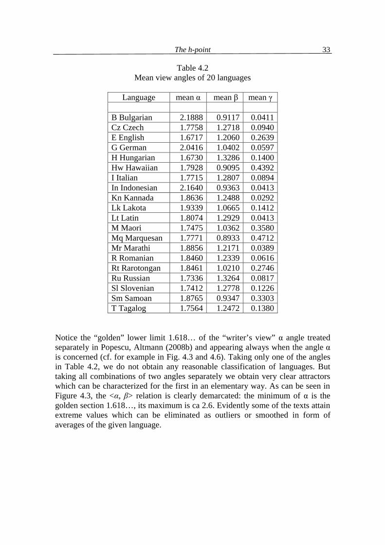
Table 4.2 Mean view angles of 20 languages

Language mean α mean β mean γ

B Bulgarian 2.1888 0.9117 0.0411 Cz Czech 1.7758 1.2718 0.0940 E English 1.6717 1.2060 0.2639 G German 2.0416 1.0402 0.0597 H Hungarian 1.6730 1.3286 0.1400 Hw Hawaiian 1.7928 0.9095 0.4392 I Italian 1.7715 1.2807 0.0894 In Indonesian 2.1640 0.9363 0.0413 Kn Kannada 1.8636 1.2488 0.0292 Lk Lakota 1.9339 1.0665 0.1412 Lt Latin 1.8074 1.2929 0.0413 M Maori 1.7475 1.0362 0.3580 Mq Marquesan 1.7771 0.8933 0.4712 Mr Marathi 1.8856 1.2171 0.0389 R Romanian 1.8460 1.2339 0.0616 Rt Rarotongan 1.8461 1.0210 0.2746 Ru Russian 1.7336 1.3264 0.0817 Sl Slovenian 1.7412 1.2778 0.1226 Sm Samoan 1.8765 0.9347 0.3303 T Tagalog 1.7564 1.2472 0.1380

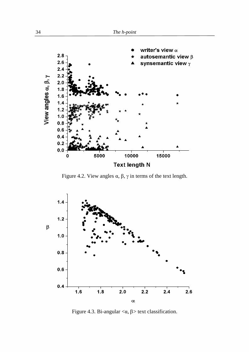
Notice the “golden” lower limit 1.618… of the “writer’s view” α angle treated separately in Popescu, Altmann (2008b) and appearing always when the angle α is concerned (cf. for example in Fig. 4.3 and 4.6). Taking only one of the angles in Table 4.2, we do not obtain any reasonable classification of languages. But taking all combinations of two angles separately we obtain very clear attractors which can be characterized for the first in an elementary way. As can be seen in Figure 4.3, the <α, β> relation is clearly demarcated: the minimum of α is the golden section 1.618…, its maximum is ca 2.6. Evidently some of the texts attain extreme values which can be eliminated as outliers or smoothed in form of averages of the given language.

The h-point

34

Figure 4.2. View angles α, β, in terms of the text length.

Figure 4.3. Bi-angular <α, > text classification.

The h-point

35

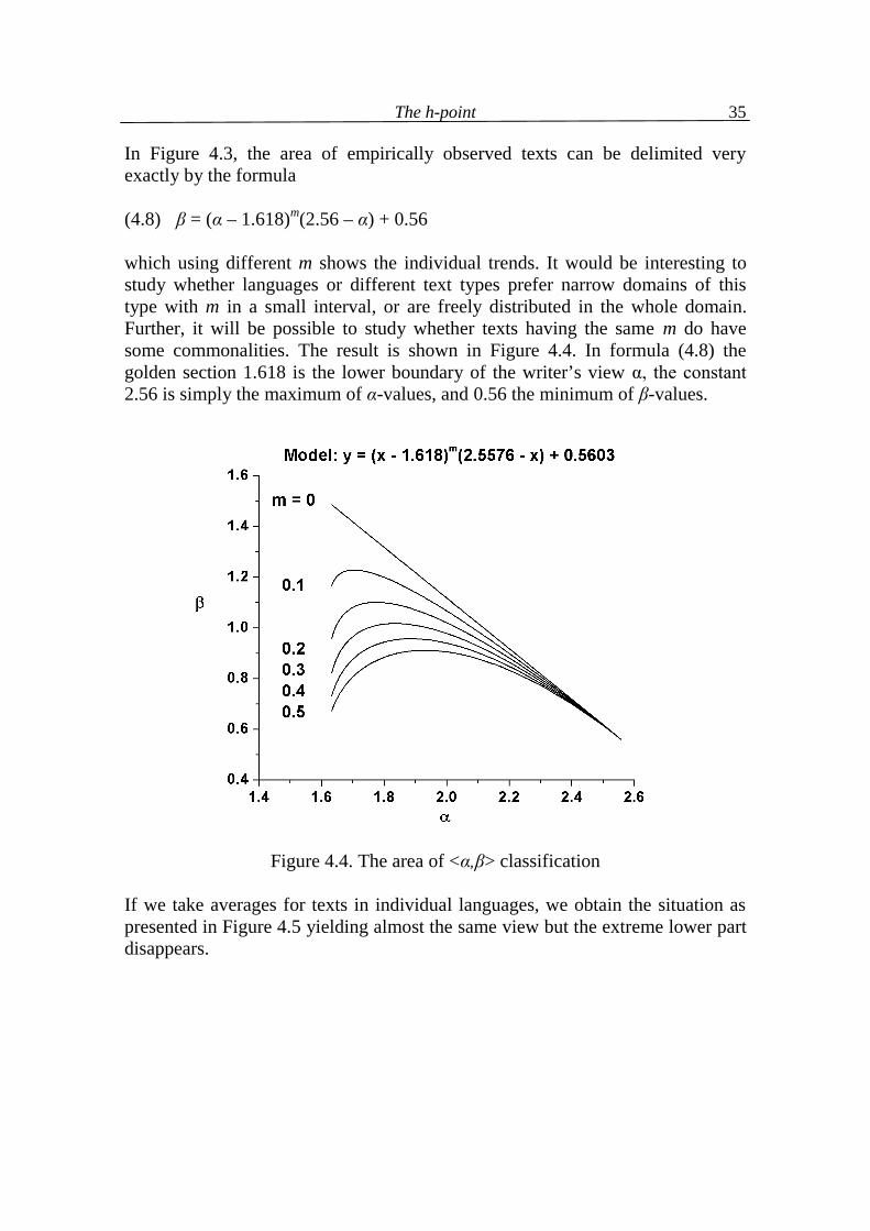
In Figure 4.3, the area of empirically observed texts can be delimited very exactly by the formula (4.8) β = (α – 1.618)m(2.56 – α) + 0.56 which using different m shows the individual trends. It would be interesting to study whether languages or different text types prefer narrow domains of this type with m in a small interval, or are freely distributed in the whole domain. Further, it will be possible to study whether texts having the same m do have some commonalities. The result is shown in Figure 4.4. In formula (4.8) the golden section 1.618 is the lower boundary of the writer’s view α, the constant 2.56 is simply the maximum of α-values, and 0.56 the minimum of β-values.

Figure 4.4. The area of <α,β> classification

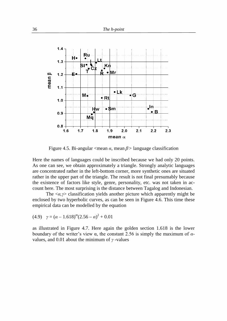
If we take averages for texts in individual languages, we obtain the situation as presented in Figure 4.5 yielding almost the same view but the extreme lower part disappears.

The h-point

36

Figure 4.5. Bi-angular <mean α, mean > language classification

Here the names of languages could be inscribed because we had only 20 points. As one can see, we obtain approximately a triangle. Strongly analytic languages are concentrated rather in the left-bottom corner, more synthetic ones are situated rather in the upper part of the triangle. The result is not final presumably because the existence of factors like style, genre, personality, etc. was not taken in ac-count here. The most surprising is the distance between Tagalog and Indonesian. The <α,γ> classification yields another picture which apparently might be enclosed by two hyperbolic curves, as can be seen in Figure 4.6. This time these empirical data can be modelled by the equation (4.9) γ = (α – 1.618)m(2.56 – α)2 + 0.01 as illustrated in Figure 4.7. Here again the golden section 1.618 is the lower boundary of the writer�s view α, the constant 2.56 is simply the maximum of α-values, and 0.01 about the minimum of γ -values

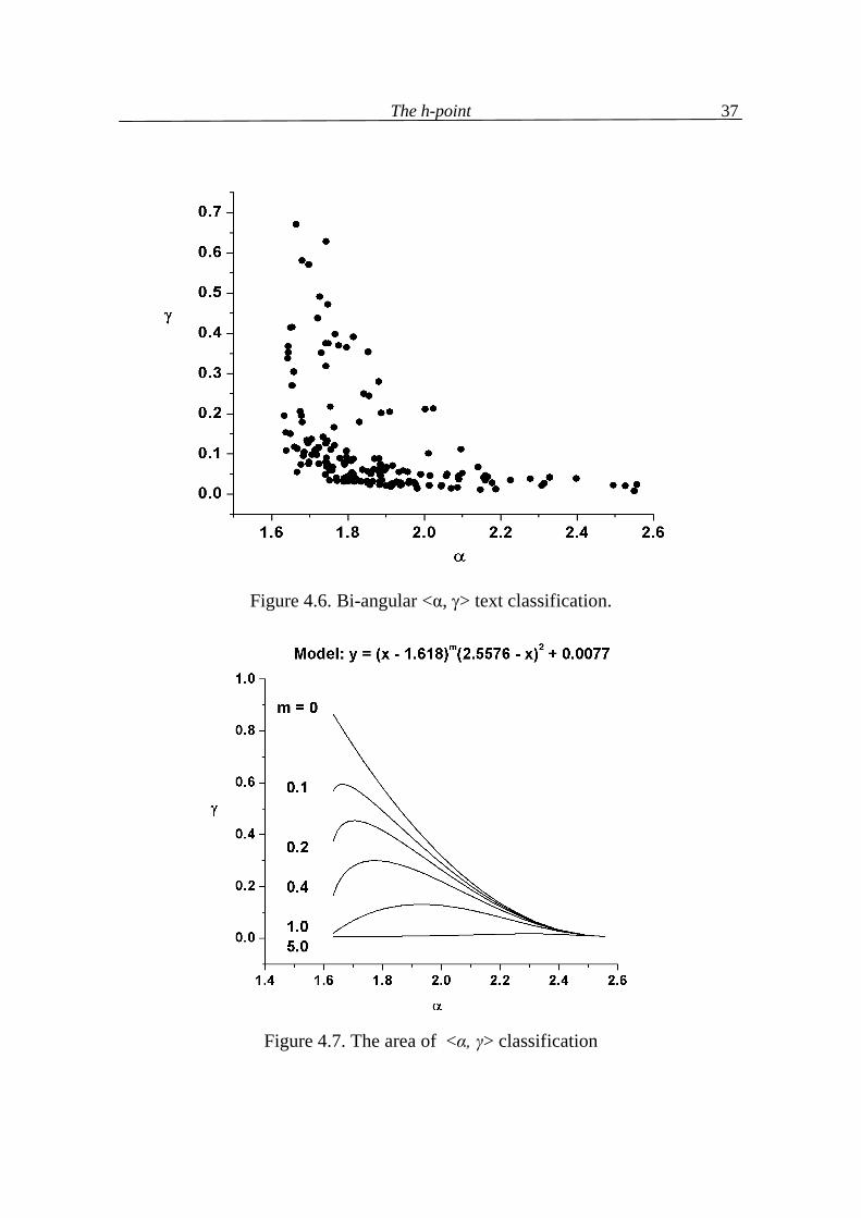
The h-point

37

Figure 4.6. Bi-angular <α, > text classification.

Figure 4.7. The area of <α, γ> classification

The h-point

38

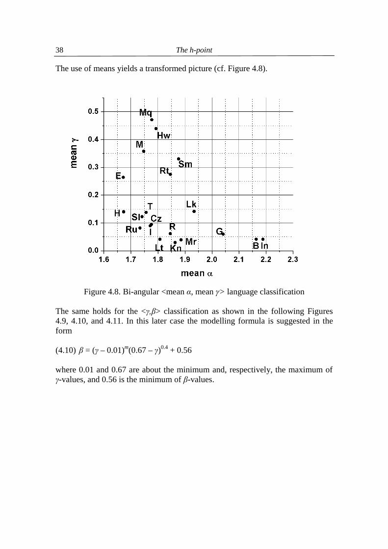
The use of means yields a transformed picture (cf. Figure 4.8).

Figure 4.8. Bi-angular <mean α, mean > language classification

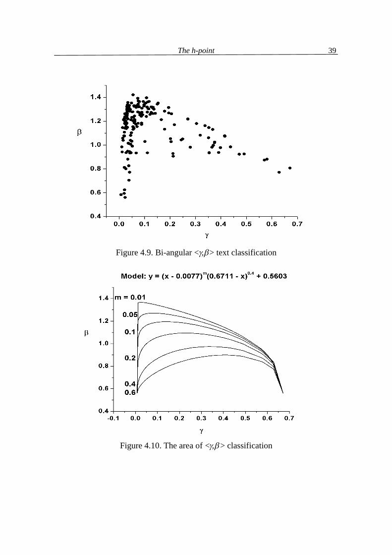
The same holds for the <γ,β> classification as shown in the following Figures 4.9, 4.10, and 4.11. In this later case the modelling formula is suggested in the form (4.10) β = (γ – 0.01)m(0.67 – γ)0.4 + 0.56 where 0.01 and 0.67 are about the minimum and, respectively, the maximum of γ-values, and 0.56 is the minimum of β-values.

The h-point

39

Figure 4.9. Bi-angular <> text classification

Figure 4.10. The area of <> classification

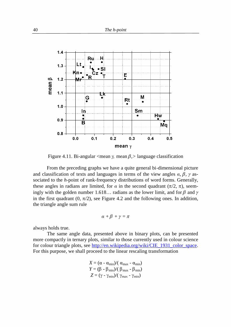
The h-point

40

Figure 4.11. Bi-angular <mean mean ,> language classification

From the preceding graphs we have a quite general bi-dimensional picture and classification of texts and languages in terms of the view angles α, , as-sociated to the h-point of rank-frequency distributions of word forms. Generally, these angles in radians are limited, for α in the second quadrant (/2, ), seem-ingly with the golden number 1.618… radians as the lower limit, and for and in the first quadrant (0, /2), see Figure 4.2 and the following ones. In addition, the triangle angle sum rule

α + + =

always holds true. The same angle data, presented above in binary plots, can be presented

more compactly in ternary plots, similar to those currently used in colour science for colour triangle plots, see http://en.wikipedia.org/wiki/CIE_1931_color_space. For this purpose, we shall proceed to the linear rescaling transformation

X = (α - αmin)/( αmax - αmin) Y = ( - min)/( max - min) Z = ( - min)/( max - min)

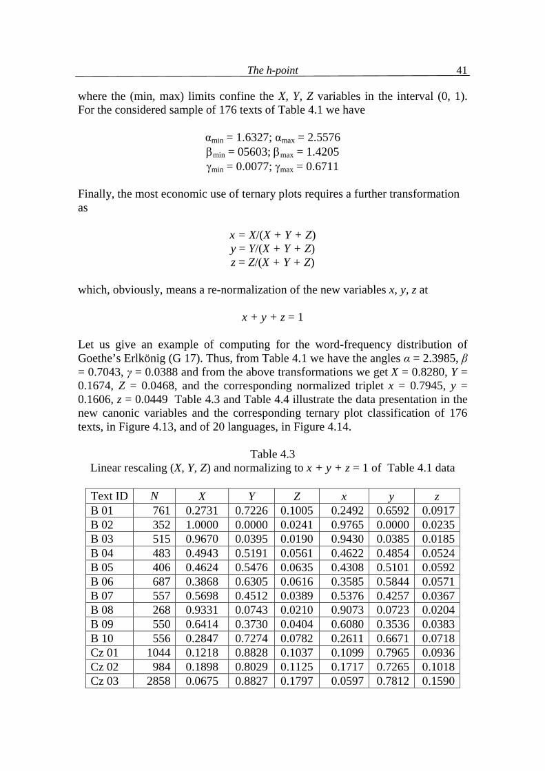
The h-point

41

where the (min, max) limits confine the X, Y, Z variables in the interval (0, 1). For the considered sample of 176 texts of Table 4.1 we have

αmin = 1.6327; αmax = 2.5576 min = 05603; max = 1.4205 min = 0.0077; max = 0.6711

Finally, the most economic use of ternary plots requires a further transformation as

x = X/(X + Y + Z) y = Y/(X + Y + Z) z = Z/(X + Y + Z)

which, obviously, means a re-normalization of the new variables x, y, z at

x + y + z = 1 Let us give an example of computing for the word-frequency distribution of Goethe’s Erlkönig (G 17). Thus, from Table 4.1 we have the angles α = 2.3985, β = 0.7043, γ = 0.0388 and from the above transformations we get X = 0.8280, Y = 0.1674, Z = 0.0468, and the corresponding normalized triplet x = 0.7945, y = 0.1606, z = 0.0449 Table 4.3 and Table 4.4 illustrate the data presentation in the new canonic variables and the corresponding ternary plot classification of 176 texts, in Figure 4.13, and of 20 languages, in Figure 4.14.

Table 4.3 Linear rescaling (X, Y, Z) and normalizing to x + y + z = 1 of Table 4.1 data

Text ID N X Y Z x y z B 01 761 0.2731 0.7226 0.1005 0.2492 0.6592 0.0917 B 02 352 1.0000 0.0000 0.0241 0.9765 0.0000 0.0235 B 03 515 0.9670 0.0395 0.0190 0.9430 0.0385 0.0185 B 04 483 0.4943 0.5191 0.0561 0.4622 0.4854 0.0524 B 05 406 0.4624 0.5476 0.0635 0.4308 0.5101 0.0592 B 06 687 0.3868 0.6305 0.0616 0.3585 0.5844 0.0571 B 07 557 0.5698 0.4512 0.0389 0.5376 0.4257 0.0367 B 08 268 0.9331 0.0743 0.0210 0.9073 0.0723 0.0204 B 09 550 0.6414 0.3730 0.0404 0.6080 0.3536 0.0383 B 10 556 0.2847 0.7274 0.0782 0.2611 0.6671 0.0718 Cz 01 1044 0.1218 0.8828 0.1037 0.1099 0.7965 0.0936 Cz 02 984 0.1898 0.8029 0.1125 0.1717 0.7265 0.1018 Cz 03 2858 0.0675 0.8827 0.1797 0.0597 0.7812 0.1590

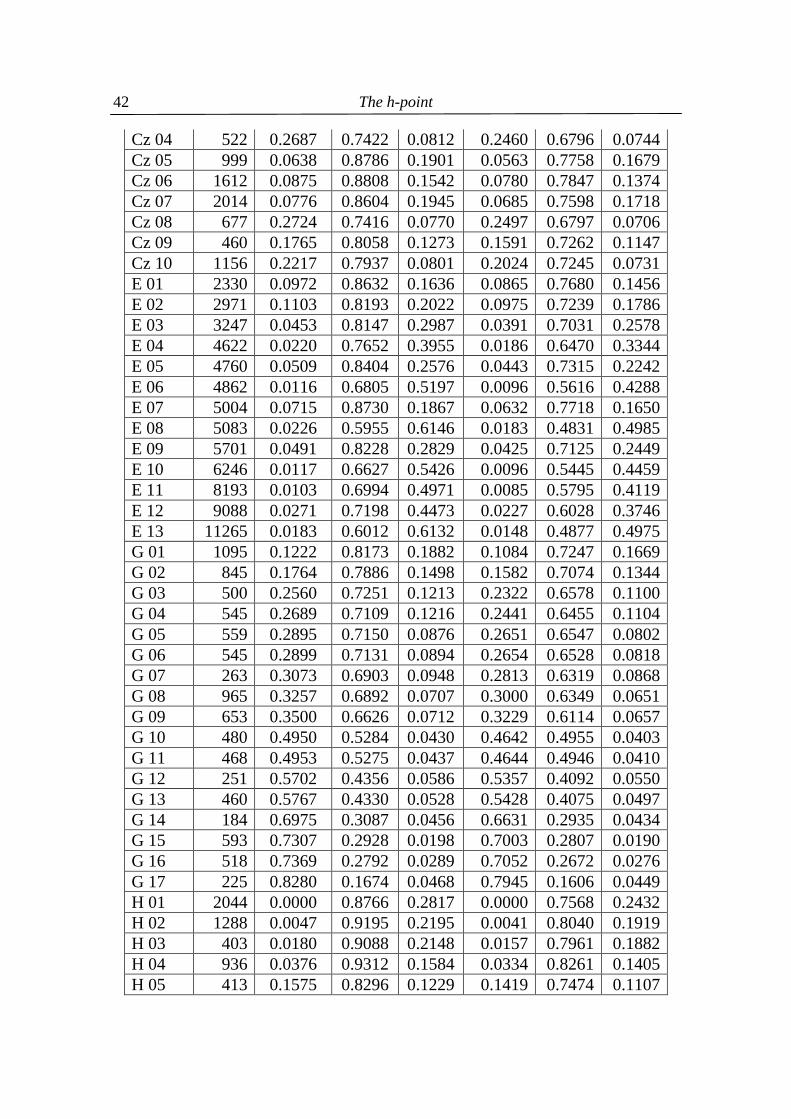
The h-point

42

Cz 04 522 0.2687 0.7422 0.0812 0.2460 0.6796 0.0744 Cz 05 999 0.0638 0.8786 0.1901 0.0563 0.7758 0.1679 Cz 06 1612 0.0875 0.8808 0.1542 0.0780 0.7847 0.1374 Cz 07 2014 0.0776 0.8604 0.1945 0.0685 0.7598 0.1718 Cz 08 677 0.2724 0.7416 0.0770 0.2497 0.6797 0.0706 Cz 09 460 0.1765 0.8058 0.1273 0.1591 0.7262 0.1147 Cz 10 1156 0.2217 0.7937 0.0801 0.2024 0.7245 0.0731 E 01 2330 0.0972 0.8632 0.1636 0.0865 0.7680 0.1456 E 02 2971 0.1103 0.8193 0.2022 0.0975 0.7239 0.1786 E 03 3247 0.0453 0.8147 0.2987 0.0391 0.7031 0.2578 E 04 4622 0.0220 0.7652 0.3955 0.0186 0.6470 0.3344 E 05 4760 0.0509 0.8404 0.2576 0.0443 0.7315 0.2242 E 06 4862 0.0116 0.6805 0.5197 0.0096 0.5616 0.4288 E 07 5004 0.0715 0.8730 0.1867 0.0632 0.7718 0.1650 E 08 5083 0.0226 0.5955 0.6146 0.0183 0.4831 0.4985 E 09 5701 0.0491 0.8228 0.2829 0.0425 0.7125 0.2449 E 10 6246 0.0117 0.6627 0.5426 0.0096 0.5445 0.4459 E 11 8193 0.0103 0.6994 0.4971 0.0085 0.5795 0.4119 E 12 9088 0.0271 0.7198 0.4473 0.0227 0.6028 0.3746 E 13 11265 0.0183 0.6012 0.6132 0.0148 0.4877 0.4975 G 01 1095 0.1222 0.8173 0.1882 0.1084 0.7247 0.1669 G 02 845 0.1764 0.7886 0.1498 0.1582 0.7074 0.1344 G 03 500 0.2560 0.7251 0.1213 0.2322 0.6578 0.1100 G 04 545 0.2689 0.7109 0.1216 0.2441 0.6455 0.1104 G 05 559 0.2895 0.7150 0.0876 0.2651 0.6547 0.0802 G 06 545 0.2899 0.7131 0.0894 0.2654 0.6528 0.0818 G 07 263 0.3073 0.6903 0.0948 0.2813 0.6319 0.0868 G 08 965 0.3257 0.6892 0.0707 0.3000 0.6349 0.0651 G 09 653 0.3500 0.6626 0.0712 0.3229 0.6114 0.0657 G 10 480 0.4950 0.5284 0.0430 0.4642 0.4955 0.0403 G 11 468 0.4953 0.5275 0.0437 0.4644 0.4946 0.0410 G 12 251 0.5702 0.4356 0.0586 0.5357 0.4092 0.0550 G 13 460 0.5767 0.4330 0.0528 0.5428 0.4075 0.0497 G 14 184 0.6975 0.3087 0.0456 0.6631 0.2935 0.0434 G 15 593 0.7307 0.2928 0.0198 0.7003 0.2807 0.0190 G 16 518 0.7369 0.2792 0.0289 0.7052 0.2672 0.0276 G 17 225 0.8280 0.1674 0.0468 0.7945 0.1606 0.0449 H 01 2044 0.0000 0.8766 0.2817 0.0000 0.7568 0.2432 H 02 1288 0.0047 0.9195 0.2195 0.0041 0.8040 0.1919 H 03 403 0.0180 0.9088 0.2148 0.0157 0.7961 0.1882 H 04 936 0.0376 0.9312 0.1584 0.0334 0.8261 0.1405 H 05 413 0.1575 0.8296 0.1229 0.1419 0.7474 0.1107

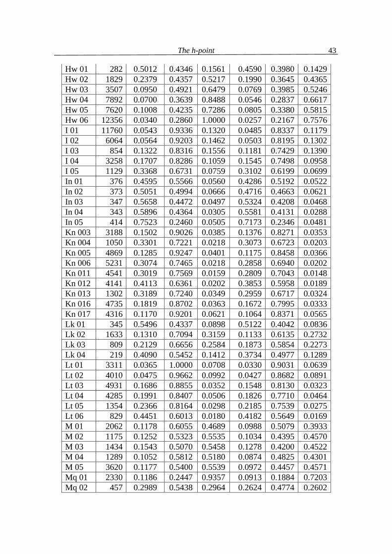
The h-point

43

Hw 01 282 0.5012 0.4346 0.1561 0.4590 0.3980 0.1429 Hw 02 1829 0.2379 0.4357 0.5217 0.1990 0.3645 0.4365 Hw 03 3507 0.0950 0.4921 0.6479 0.0769 0.3985 0.5246 Hw 04 7892 0.0700 0.3639 0.8488 0.0546 0.2837 0.6617 Hw 05 7620 0.1008 0.4235 0.7286 0.0805 0.3380 0.5815 Hw 06 12356 0.0340 0.2860 1.0000 0.0257 0.2167 0.7576 I 01 11760 0.0543 0.9336 0.1320 0.0485 0.8337 0.1179 I 02 6064 0.0564 0.9203 0.1462 0.0503 0.8195 0.1302 I 03 854 0.1322 0.8316 0.1556 0.1181 0.7429 0.1390 I 04 3258 0.1707 0.8286 0.1059 0.1545 0.7498 0.0958 I 05 1129 0.3368 0.6731 0.0759 0.3102 0.6199 0.0699 In 01 376 0.4595 0.5566 0.0560 0.4286 0.5192 0.0522 In 02 373 0.5051 0.4994 0.0666 0.4716 0.4663 0.0621 In 03 347 0.5658 0.4472 0.0497 0.5324 0.4208 0.0468 In 04 343 0.5896 0.4364 0.0305 0.5581 0.4131 0.0288 In 05 414 0.7523 0.2460 0.0505 0.7173 0.2346 0.0481 Kn 003 3188 0.1502 0.9026 0.0385 0.1376 0.8271 0.0353 Kn 004 1050 0.3301 0.7221 0.0218 0.3073 0.6723 0.0203 Kn 005 4869 0.1285 0.9247 0.0401 0.1175 0.8458 0.0366 Kn 006 5231 0.3074 0.7465 0.0218 0.2858 0.6940 0.0202 Kn 011 4541 0.3019 0.7569 0.0159 0.2809 0.7043 0.0148 Kn 012 4141 0.4113 0.6361 0.0202 0.3853 0.5958 0.0189 Kn 013 1302 0.3189 0.7240 0.0349 0.2959 0.6717 0.0324 Kn 016 4735 0.1819 0.8702 0.0363 0.1672 0.7995 0.0333 Kn 017 4316 0.1170 0.9201 0.0621 0.1064 0.8371 0.0565 Lk 01 345 0.5496 0.4337 0.0898 0.5122 0.4042 0.0836 Lk 02 1633 0.1310 0.7094 0.3159 0.1133 0.6135 0.2732 Lk 03 809 0.2129 0.6656 0.2584 0.1873 0.5854 0.2273 Lk 04 219 0.4090 0.5452 0.1412 0.3734 0.4977 0.1289 Lt 01 3311 0.0365 1.0000 0.0708 0.0330 0.9031 0.0639 Lt 02 4010 0.0475 0.9662 0.0992 0.0427 0.8682 0.0891 Lt 03 4931 0.1686 0.8855 0.0352 0.1548 0.8130 0.0323 Lt 04 4285 0.1991 0.8407 0.0506 0.1826 0.7710 0.0464 Lt 05 1354 0.2366 0.8164 0.0298 0.2185 0.7539 0.0275 Lt 06 829 0.4451 0.6013 0.0180 0.4182 0.5649 0.0169 M 01 2062 0.1178 0.6055 0.4689 0.0988 0.5079 0.3933 M 02 1175 0.1252 0.5323 0.5535 0.1034 0.4395 0.4570 M 03 1434 0.1543 0.5070 0.5458 0.1278 0.4200 0.4522 M 04 1289 0.1052 0.5812 0.5180 0.0874 0.4825 0.4301 M 05 3620 0.1177 0.5400 0.5539 0.0972 0.4457 0.4571 Mq 01 2330 0.1186 0.2447 0.9357 0.0913 0.1884 0.7203 Mq 02 457 0.2989 0.5438 0.2964 0.2624 0.4774 0.2602

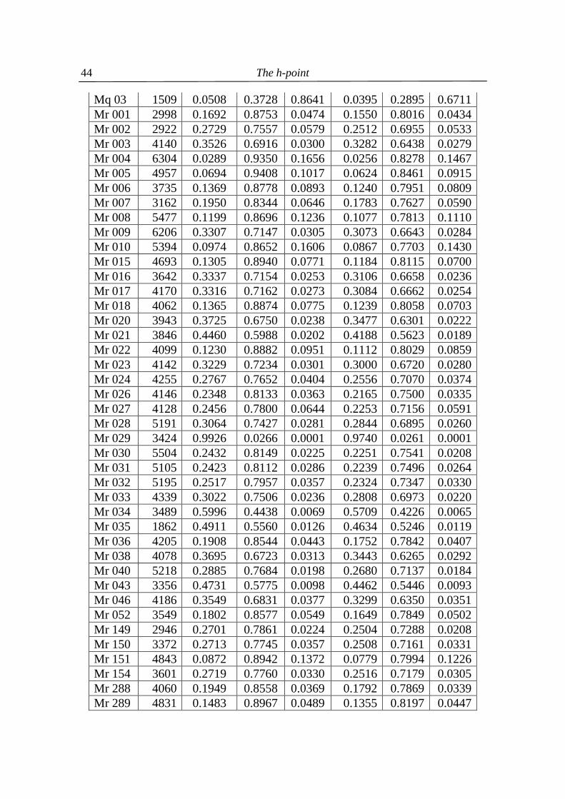
The h-point

44

Mq 03 1509 0.0508 0.3728 0.8641 0.0395 0.2895 0.6711 Mr 001 2998 0.1692 0.8753 0.0474 0.1550 0.8016 0.0434 Mr 002 2922 0.2729 0.7557 0.0579 0.2512 0.6955 0.0533 Mr 003 4140 0.3526 0.6916 0.0300 0.3282 0.6438 0.0279 Mr 004 6304 0.0289 0.9350 0.1656 0.0256 0.8278 0.1467 Mr 005 4957 0.0694 0.9408 0.1017 0.0624 0.8461 0.0915 Mr 006 3735 0.1369 0.8778 0.0893 0.1240 0.7951 0.0809 Mr 007 3162 0.1950 0.8344 0.0646 0.1783 0.7627 0.0590 Mr 008 5477 0.1199 0.8696 0.1236 0.1077 0.7813 0.1110 Mr 009 6206 0.3307 0.7147 0.0305 0.3073 0.6643 0.0284 Mr 010 5394 0.0974 0.8652 0.1606 0.0867 0.7703 0.1430 Mr 015 4693 0.1305 0.8940 0.0771 0.1184 0.8115 0.0700 Mr 016 3642 0.3337 0.7154 0.0253 0.3106 0.6658 0.0236 Mr 017 4170 0.3316 0.7162 0.0273 0.3084 0.6662 0.0254 Mr 018 4062 0.1365 0.8874 0.0775 0.1239 0.8058 0.0703 Mr 020 3943 0.3725 0.6750 0.0238 0.3477 0.6301 0.0222 Mr 021 3846 0.4460 0.5988 0.0202 0.4188 0.5623 0.0189 Mr 022 4099 0.1230 0.8882 0.0951 0.1112 0.8029 0.0859 Mr 023 4142 0.3229 0.7234 0.0301 0.3000 0.6720 0.0280 Mr 024 4255 0.2767 0.7652 0.0404 0.2556 0.7070 0.0374 Mr 026 4146 0.2348 0.8133 0.0363 0.2165 0.7500 0.0335 Mr 027 4128 0.2456 0.7800 0.0644 0.2253 0.7156 0.0591 Mr 028 5191 0.3064 0.7427 0.0281 0.2844 0.6895 0.0260 Mr 029 3424 0.9926 0.0266 0.0001 0.9740 0.0261 0.0001 Mr 030 5504 0.2432 0.8149 0.0225 0.2251 0.7541 0.0208 Mr 031 5105 0.2423 0.8112 0.0286 0.2239 0.7496 0.0264 Mr 032 5195 0.2517 0.7957 0.0357 0.2324 0.7347 0.0330 Mr 033 4339 0.3022 0.7506 0.0236 0.2808 0.6973 0.0220 Mr 034 3489 0.5996 0.4438 0.0069 0.5709 0.4226 0.0065 Mr 035 1862 0.4911 0.5560 0.0126 0.4634 0.5246 0.0119 Mr 036 4205 0.1908 0.8544 0.0443 0.1752 0.7842 0.0407 Mr 038 4078 0.3695 0.6723 0.0313 0.3443 0.6265 0.0292 Mr 040 5218 0.2885 0.7684 0.0198 0.2680 0.7137 0.0184 Mr 043 3356 0.4731 0.5775 0.0098 0.4462 0.5446 0.0093 Mr 046 4186 0.3549 0.6831 0.0377 0.3299 0.6350 0.0351 Mr 052 3549 0.1802 0.8577 0.0549 0.1649 0.7849 0.0502 Mr 149 2946 0.2701 0.7861 0.0224 0.2504 0.7288 0.0208 Mr 150 3372 0.2713 0.7745 0.0357 0.2508 0.7161 0.0331 Mr 151 4843 0.0872 0.8942 0.1372 0.0779 0.7994 0.1226 Mr 154 3601 0.2719 0.7760 0.0330 0.2516 0.7179 0.0305 Mr 288 4060 0.1949 0.8558 0.0369 0.1792 0.7869 0.0339 Mr 289 4831 0.1483 0.8967 0.0489 0.1355 0.8197 0.0447

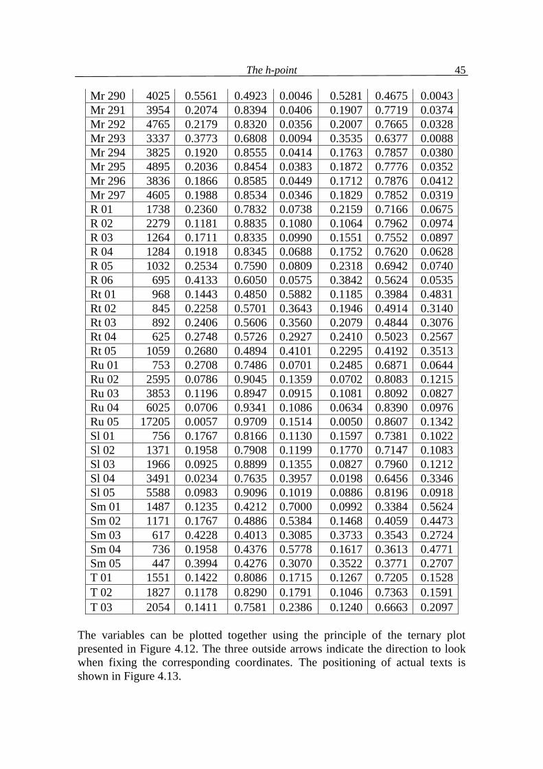
The h-point

45

Mr 290 4025 0.5561 0.4923 0.0046 0.5281 0.4675 0.0043 Mr 291 3954 0.2074 0.8394 0.0406 0.1907 0.7719 0.0374 Mr 292 4765 0.2179 0.8320 0.0356 0.2007 0.7665 0.0328 Mr 293 3337 0.3773 0.6808 0.0094 0.3535 0.6377 0.0088 Mr 294 3825 0.1920 0.8555 0.0414 0.1763 0.7857 0.0380 Mr 295 4895 0.2036 0.8454 0.0383 0.1872 0.7776 0.0352 Mr 296 3836 0.1866 0.8585 0.0449 0.1712 0.7876 0.0412 Mr 297 4605 0.1988 0.8534 0.0346 0.1829 0.7852 0.0319 R 01 1738 0.2360 0.7832 0.0738 0.2159 0.7166 0.0675 R 02 2279 0.1181 0.8835 0.1080 0.1064 0.7962 0.0974 R 03 1264 0.1711 0.8335 0.0990 0.1551 0.7552 0.0897 R 04 1284 0.1918 0.8345 0.0688 0.1752 0.7620 0.0628 R 05 1032 0.2534 0.7590 0.0809 0.2318 0.6942 0.0740 R 06 695 0.4133 0.6050 0.0575 0.3842 0.5624 0.0535 Rt 01 968 0.1443 0.4850 0.5882 0.1185 0.3984 0.4831 Rt 02 845 0.2258 0.5701 0.3643 0.1946 0.4914 0.3140 Rt 03 892 0.2406 0.5606 0.3560 0.2079 0.4844 0.3076 Rt 04 625 0.2748 0.5726 0.2927 0.2410 0.5023 0.2567 Rt 05 1059 0.2680 0.4894 0.4101 0.2295 0.4192 0.3513 Ru 01 753 0.2708 0.7486 0.0701 0.2485 0.6871 0.0644 Ru 02 2595 0.0786 0.9045 0.1359 0.0702 0.8083 0.1215 Ru 03 3853 0.1196 0.8947 0.0915 0.1081 0.8092 0.0827 Ru 04 6025 0.0706 0.9341 0.1086 0.0634 0.8390 0.0976 Ru 05 17205 0.0057 0.9709 0.1514 0.0050 0.8607 0.1342 Sl 01 756 0.1767 0.8166 0.1130 0.1597 0.7381 0.1022 Sl 02 1371 0.1958 0.7908 0.1199 0.1770 0.7147 0.1083 Sl 03 1966 0.0925 0.8899 0.1355 0.0827 0.7960 0.1212 Sl 04 3491 0.0234 0.7635 0.3957 0.0198 0.6456 0.3346 Sl 05 5588 0.0983 0.9096 0.1019 0.0886 0.8196 0.0918 Sm 01 1487 0.1235 0.4212 0.7000 0.0992 0.3384 0.5624 Sm 02 1171 0.1767 0.4886 0.5384 0.1468 0.4059 0.4473 Sm 03 617 0.4228 0.4013 0.3085 0.3733 0.3543 0.2724 Sm 04 736 0.1958 0.4376 0.5778 0.1617 0.3613 0.4771 Sm 05 447 0.3994 0.4276 0.3070 0.3522 0.3771 0.2707 T 01 1551 0.1422 0.8086 0.1715 0.1267 0.7205 0.1528 T 02 1827 0.1178 0.8290 0.1791 0.1046 0.7363 0.1591 T 03 2054 0.1411 0.7581 0.2386 0.1240 0.6663 0.2097

The variables can be plotted together using the principle of the ternary plot presented in Figure 4.12. The three outside arrows indicate the direction to look when fixing the corresponding coordinates. The positioning of actual texts is shown in Figure 4.13.

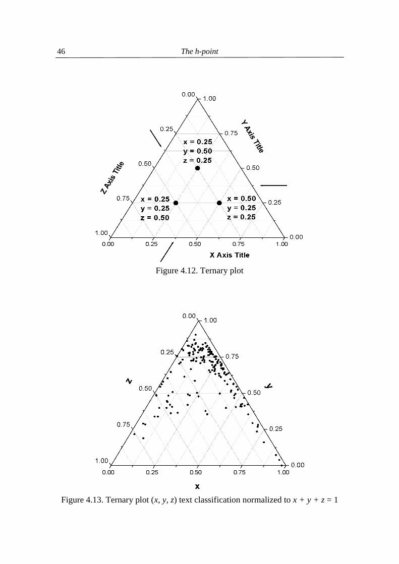
The h-point

46

Figure 4.12. Ternary plot

Figure 4.13. Ternary plot (x, y, z) text classification normalized to x + y + z = 1

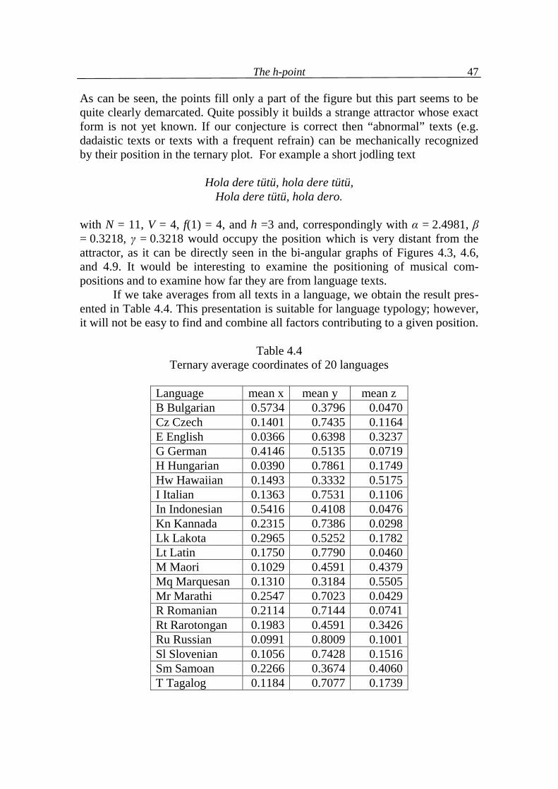
The h-point

47

As can be seen, the points fill only a part of the figure but this part seems to be quite clearly demarcated. Quite possibly it builds a strange attractor whose exact form is not yet known. If our conjecture is correct then “abnormal” texts (e.g. dadaistic texts or texts with a frequent refrain) can be mechanically recognized by their position in the ternary plot. For example a short jodling text

Hola dere tütü, hola dere tütü, Hola dere tütü, hola dero.

with N = 11, V = 4, f(1) = 4, and h =3 and, correspondingly with α = 2.4981, β = 0.3218, γ = 0.3218 would occupy the position which is very distant from the attractor, as it can be directly seen in the bi-angular graphs of Figures 4.3, 4.6, and 4.9. It would be interesting to examine the positioning of musical com-positions and to examine how far they are from language texts. If we take averages from all texts in a language, we obtain the result pres-ented in Table 4.4. This presentation is suitable for language typology; however, it will not be easy to find and combine all factors contributing to a given position.

Table 4.4 Ternary average coordinates of 20 languages

Language mean x mean y mean z B Bulgarian 0.5734 0.3796 0.0470 Cz Czech 0.1401 0.7435 0.1164 E English 0.0366 0.6398 0.3237 G German 0.4146 0.5135 0.0719 H Hungarian 0.0390 0.7861 0.1749 Hw Hawaiian 0.1493 0.3332 0.5175 I Italian 0.1363 0.7531 0.1106 In Indonesian 0.5416 0.4108 0.0476 Kn Kannada 0.2315 0.7386 0.0298 Lk Lakota 0.2965 0.5252 0.1782 Lt Latin 0.1750 0.7790 0.0460 M Maori 0.1029 0.4591 0.4379 Mq Marquesan 0.1310 0.3184 0.5505 Mr Marathi 0.2547 0.7023 0.0429 R Romanian 0.2114 0.7144 0.0741 Rt Rarotongan 0.1983 0.4591 0.3426 Ru Russian 0.0991 0.8009 0.1001 Sl Slovenian 0.1056 0.7428 0.1516 Sm Samoan 0.2266 0.3674 0.4060 T Tagalog 0.1184 0.7077 0.1739

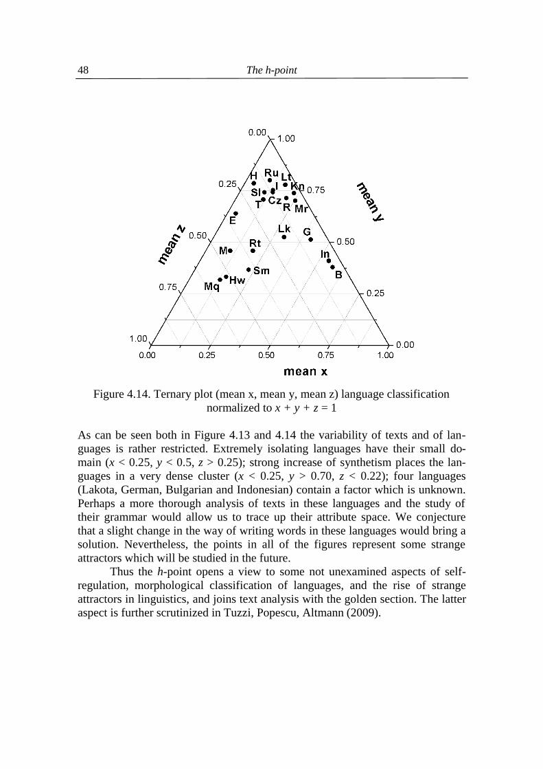
The h-point

48

Figure 4.14. Ternary plot (mean x, mean y, mean z) language classification

normalized to x + y + z = 1

As can be seen both in Figure 4.13 and 4.14 the variability of texts and of lan-guages is rather restricted. Extremely isolating languages have their small do-main (x < 0.25, y < 0.5, z > 0.25); strong increase of synthetism places the lan-guages in a very dense cluster (x < 0.25, y > 0.70, z < 0.22); four languages (Lakota, German, Bulgarian and Indonesian) contain a factor which is unknown. Perhaps a more thorough analysis of texts in these languages and the study of their grammar would allow us to trace up their attribute space. We conjecture that a slight change in the way of writing words in these languages would bring a solution. Nevertheless, the points in all of the figures represent some strange attractors which will be studied in the future. Thus the h-point opens a view to some not unexamined aspects of self-regulation, morphological classification of languages, and the rise of strange attractors in linguistics, and joins text analysis with the golden section. The latter aspect is further scrutinized in Tuzzi, Popescu, Altmann (2009).

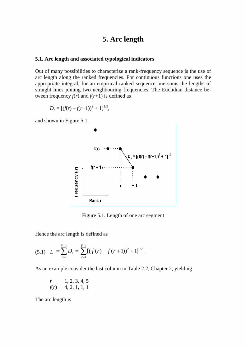
5. Arc length

5.1. Arc length and associated typological indicators Out of many possibilities to characterize a rank-frequency sequence is the use of arc length along the ranked frequencies. For continuous functions one uses the appropriate integral, for an empirical ranked sequence one sums the lengths of straight lines joining two neighbouring frequencies. The Euclidian distance be-tween frequency f(r) and f(r+1) is defined as Dr = [(f(r) – f(r+1))2 + 1]1/2, and shown in Figure 5.1.

Figure 5.1. Length of one arc segment Hence the arc length is defined as

(5.1) L 1 1

2 1/2

1 1[( ( ) ( 1)) 1]

V V

rr r

D f r f r

.

As an example consider the last column in Table 2.2, Chapter 2, yielding r 1, 2, 3, 4, 5 f(r) 4, 2, 1, 1, 1 The arc length is

Arc length

50

[(4 – 2)2 + 1]1/2 + [(2 – 1)2 + 1]1/2 + [(1 – 1)2 + 1]1/2 + [(1 – 1)2 + 1]1/2 = 5.650. However, arc length itself is not sufficient for characterization because it depends on text length N whose simplest representative is the greatest frequency f(1), and on the vocabulary (or inventory of forms) level the size V. In order to warrant comparability, the authors proposed four different indicators which may be used to characterize the rank-frequency sequence (Popescu, Mačutek, Altmann 2008). They are as follows

(5.2) 1max

LBL

,

where 2 1/2

max [( (1) 1) 1] 2L f V representing the case when f(1) > 1 and all other f(r) = 1. This is a simply rela- tivized arc length. Another normalization can be performed by defining

(5.3) min

2max min

L LBL L

,

where 2 2 1/2

min [( 1) ( (1) 1) ]L V f represents the length of the straight line joining the points P1 (V, 1) and P2 (1, f(1)), see Figure 4.1 of Chapter 4. For the above example we would obtain Lmax = [(4 – 1)2 + 1]1/2 + 5 – 2 = 6.162 Lmin = [(5 – 1)2 + (4 – 1)2]1/2 = 5.000. Hence B1 = 5.650/6.162 = 0.917 B2 = (5.650 – 5.000)/( 6.162 – 5.000) = 0.559. Both indicators lie in the interval <0, 1>. Using the individual components of Lmin (that is (V – 1) or (f(1) – 1)) one can set up two further indicators, namely

(5.4) 31VB

L

Arc length

51

and

(5.5) 4(1) 1fBL

.

Since L is always greater than V-1 and f(1)-1, these last indicators lie in the

interval <0,1>, too. For our example we have 3

5 10.708

5.650B

and

4

4 10.531

5.650B

.

In order to be able to test differences between particular indicators, we derive estimations of their variances. We use the well known delta method (cf. Oehlert 1992) based on a linear approximation of a non-linear function. V and f(1) are considered to be fixed. In the following, f1,…fV are random variables (i.e., functions, not numbers, which are denoted f(1),…,f(V)).

L is a function of frequencies, i.e., 11

2 21 1

1

, , 1V

V r rr

L L f f f f

.

Approximating the function by its first order Taylor polynomial (ff is a constant, hence its derivative is zero), we obtain

(5.6) 1 1, , , ,V VL f f L 2 22

V VV

L Lf ff f

,

where θ = (θ1,… θV) is the mean vector of 1, , Vf f (i.e., E(f1) =

1, , V VE f ). Denote

(5.7)

1 12 2

1 11 1r rr r

rr r rr r

Laf

, 1,,3,2 Vr ,

(5.8)

12

1 1VV

VV VV

Laf

.

Inserting the derivatives into (5.6) we obtain

1 12

, , , ,V

V V k k kk

L f f L a f

Arc length

52

and an approximation of the variance

(5.9) 2

2

V

r rr

Var L a Var f

+2 1

2 1,

V V

r s r sr s r

a a Cov f f

.

Variances and covariances from the last formula can be estimated from the prop-erties of the multinomial distribution. We have N words in V categories with the fixed number of words in the first category, resulting in the conditional prob-ability (5.10)

( )(2)

22 1

1

(1) !2 , , 1

(2)! ( )! 1 1

f Vf

VV

V

N f p pP f f f f V f f

f f V p p

which means that the conditional distribution is again multinomial having now

the parameters 2

1 1

(1), , ,1 1

Vp pN f

p p

, which means that for Vr ,,2 we

have

(5.11) 1

( ) (1)1

rr

pE f N fp

(note that r rE f ),

(5.12) 1 1

(1) 11 1

r rr

p pVar f N fp p

,

(5.13) 21

, (1)1

r sr s

p pCov f f N fp

.

As f(1) is a constant, it holds (1) (1)E f f . The values of N and f(1) are

known, the others can be estimated as ( )ˆ k

f kp

N , k = 1,…,V, thus making

possible to estimate also

(5.14)

1 1

1 12 2

2 21 1

1 1

ˆ ˆ ˆ ˆ(1) (1)ˆ ˆ1 1

ˆˆ ˆ ˆ ˆ(1) 1 (1) 1

ˆ ˆ1 1

r r r r

r

r r r r

p p p pN f N fp p

ap p p pN f N f

p p

,

for r = 2,…,V-1 and

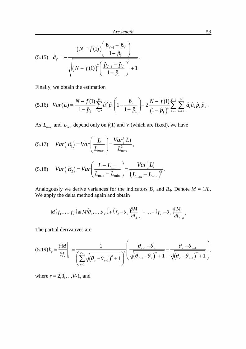
Arc length

53

(5.15)

1

12

2 1

1

ˆ ˆ(1)ˆ1

ˆˆ ˆ(1) 1

ˆ1

V V

V

V V

p pN fp

ap pN f

p

.

Finally, we obtain the estimation

(5.16)

12

22 2 11 1 1

ˆ(1) (1)ˆ ˆ ˆ ˆ ˆ ˆ( ) 1 2ˆ ˆ1 1 ˆ1

V V Vr

r r r s r sr r s r

N f p N fVar L a p a a p pp p p

.

As maxL and minL depend only on f(1) and V (which are fixed), we have

(5.17) 1 2

max max

Var LLVar B VarL L

,

(5.18)

min2 2

max min max min

Var LL LVar B VarL L L L

.

Analogously we derive variances for the indicators B3 and B4. Denote M = 1/L. We apply the delta method again and obtain

VV MffM ,,,, 11

V

VV fMf

fMf

2

22 .

The partial derivatives are

(5.19)

1 1

2 2 212

1 11

1

1

1 11

r r r rr V

r r r r rr r

r

Mb

f

,

where r = 2,3,…,V-1, and

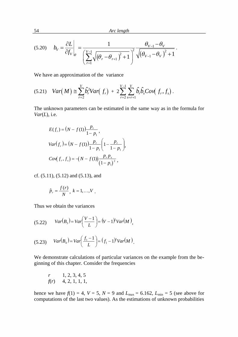
Arc length

54

(5.20)

1

2 21 2 11

1

1

11

VVV VV VV

r rr

Lbf

.

We have an approximation of the variance

(5.21) 2

2

ˆV

r rr

Var M b Var f

+ 2 1

2 1

ˆ ˆ ,V V

r s r sr s r

b b Cov f f

.

The unknown parameters can be estimated in the same way as in the formula for Var(L), i.e.

11

)1()(p

pfNfE rr

,

11 1

11

)1(p

pp

pfNfVar rrr ,

2

11)1(,

pppfNffCov sr

sr ,

cf. (5.11), (5.12) and (5.13), and

Nrfpr)(ˆ , Vk ,,1 .

Thus we obtain the variances

(5.22) MVarVL

VVarBVar 23 11

,

(5.23) MVarfL

fVarBVar 21

14 11

.

We demonstrate calculations of particular variances on the example from the be-ginning of this chapter. Consider the frequencies

r 1, 2, 3, 4, 5 f(r) 4, 2, 1, 1, 1, hence we have f(1) = 4, V = 5, N = 9 and Lmax = 6.162, Lmin = 5 (see above for computations of the last two values). As the estimations of unknown probabilities

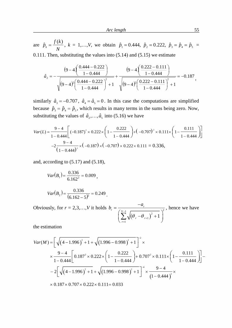
Arc length

55

are ( )ˆ k

f kp

N , k = 1,…,V, we obtain 1ˆ 0.444,p 2ˆ 0.222,p 3 4ˆ ˆp p 5p̂ =

0.111. Then, substituting the values into (5.14) and (5.15) we estimate

187.0

1444.01

111.0222.049

444.01111.0222.049

1444.01

222.0444.049

444.01222.0444.049

ˆ2

22

2

2

a ,

similarly 3ˆ 0.707a , 4 5ˆ ˆ 0a a . In this case the computations are simplified because 3 4 5ˆ ˆ ˆp p p , which results in many terms in the sums being zero. Now, substituting the values of 2 5ˆ ˆ, ,a a into (5.16) we have

229 4 0.222 0.111( ) ( 0.187) 0.222 1 0.707 0.111 1

1 0.444 1 0.444 1 0.444Var L

2

9 42 0.187 0.707 0.222 0.111

1 0.444

= 0.336,

and, according to (5.17) and (5.18),

009.0162.6336.0

21 BVar ,

249.0

5162.6336.0

22

BVar .

Obviously, for r = 2,3,…,V it holds

21

21

1

1

rr V

r rr

ab

, hence we have

the estimation

22 2

2 2

42 2

2

( ) 4 1.996 1 1.996 0.998 1

9 4 0.222 0.1110.187 0.222 1 0.707 0.111 1

1 0.444 1 0.444 1 0.4449 4

2 4 1.996 1 1.996 0.998 11 0.444

0.187 0.707 0.222 0.111 0.033

Var M

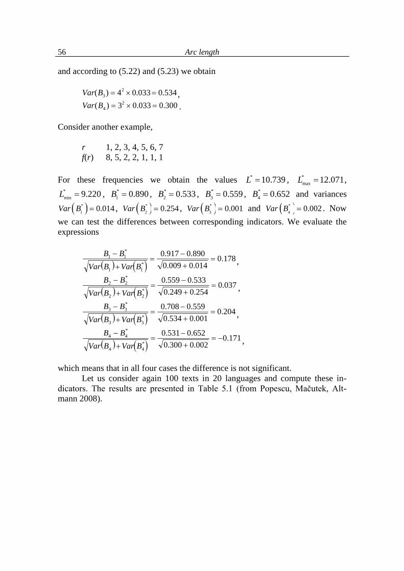
Arc length

56

and according to (5.22) and (5.23) we obtain 534.0033.04)( 2

3 BVar , 300.0033.03)( 2

4 BVar . Consider another example,

r 1, 2, 3, 4, 5, 6, 7 f(r) 8, 5, 2, 2, 1, 1, 1 For these frequencies we obtain the values * 10.739L , *

max 12.071L , *min 9.220L , *

1 0.890B , *2 0.533B , *

3 0.559B , *4 0.652B and variances

*1 0.014Var B , *

2 0.254Var B , *3 0.001Var B and *

4 0.002Var B . Now we can test the differences between corresponding indicators. We evaluate the expressions

178.0

014.0009.0890.0917.0

*11

*11

BVarBVarBB

,

037.0

254.0249.0533.0559.0

*22

*22

BVarBVarBB

,

204.0

001.0534.0559.0708.0

*33

*33

BVarBVarBB

,

171.0

002.0300.0652.0531.0

*44

*44

BVarBVarBB

,

which means that in all four cases the difference is not significant. Let us consider again 100 texts in 20 languages and compute these in-dicators. The results are presented in Table 5.1 (from Popescu, Mačutek, Alt-mann 2008).

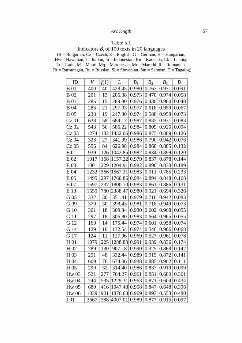
Arc length

57

Table 5.1 Indicators Bi of 100 texts in 20 languages

(B = Bulgarian, Cz = Czech, E = English, G = German, H = Hungarian, Hw = Hawaiian, I = Italian, In = Indonesian, Kn = Kannada, Lk = Lakota, Lt = Latin, M = Maori, Mq = Marquesan, Mr = Marathi, R = Romanian,

Rt = Rarotongan, Ru = Russian, Sl = Slovenian, Sm = Samoan, T = Tagalog)

ID V f(1) L B1 B2 B3 B4 B 01 400 40 428.45 0.980 0.763 0.931 0.091 B 02 201 13 205.38 0.973 0.470 0.974 0.058 B 03 285 15 289.80 0.976 0.430 0.980 0.048 B 04 286 21 297.03 0.977 0.618 0.959 0.067 B 05 238 19 247.30 0.974 0.588 0.958 0.073 Cz 01 638 58 684.17 0.987 0.835 0.931 0.083 Cz 02 543 56 586.22 0.984 0.809 0.925 0.094 Cz 03 1274 182 1432.06 0.986 0.875 0.889 0.126 Cz 04 323 27 341.99 0.986 0.790 0.942 0.076 Cz 05 556 84 626.98 0.984 0.868 0.885 0.132 E 01 939 126 1042.85 0.982 0.834 0.899 0.120 E 02 1017 168 1157.22 0.979 0.837 0.878 0.144 E 03 1001 229 1204.91 0.982 0.890 0.830 0.189 E 04 1232 366 1567.31 0.983 0.911 0.785 0.233 E 05 1495 297 1760.86 0.984 0.894 0.848 0.168 E 07 1597 237 1800.70 0.983 0.861 0.886 0.131 E 13 1659 780 2388.47 0.980 0.921 0.694 0.326 G 05 332 30 351.41 0.979 0.716 0.942 0.083 G 09 379 30 398.43 0.981 0.718 0.949 0.073 G 10 301 18 309.84 0.980 0.602 0.968 0.055 G 11 297 18 306.80 0.983 0.664 0.965 0.055 G 12 169 14 175.44 0.974 0.601 0.958 0.074 G 14 129 10 132.54 0.974 0.546 0.966 0.068 G 17 124 11 127.96 0.969 0.527 0.961 0.078 H 01 1079 225 1288.83 0.991 0.939 0.836 0.174 H 02 789 130 907.18 0.990 0.925 0.869 0.142 H 03 291 48 332.44 0.989 0.915 0.872 0.141 H 04 609 76 674.06 0.988 0.885 0.902 0.111 H 05 290 32 314.40 0.986 0.837 0.919 0.099 Hw 03 521 277 764.27 0.961 0.851 0.680 0.361 Hw 04 744 535 1229.31 0.963 0.871 0.604 0.434 Hw 05 680 416 1047.48 0.958 0.847 0.648 0.396 Hw 06 1039 901 1876.68 0.969 0.893 0.553 0.480 I 01 3667 388 4007.01 0.989 0.877 0.915 0.097

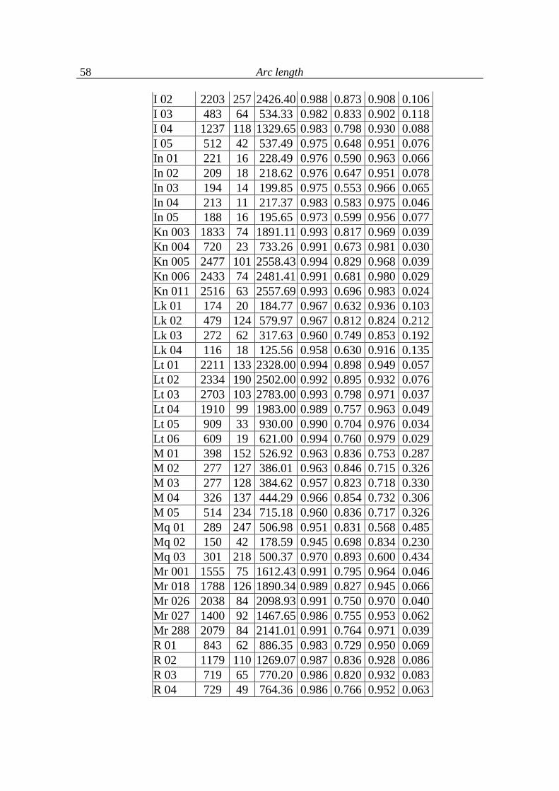
Arc length

58

I 02 2203 257 2426.40 0.988 0.873 0.908 0.106 I 03 483 64 534.33 0.982 0.833 0.902 0.118 I 04 1237 118 1329.65 0.983 0.798 0.930 0.088 I 05 512 42 537.49 0.975 0.648 0.951 0.076 In 01 221 16 228.49 0.976 0.590 0.963 0.066 In 02 209 18 218.62 0.976 0.647 0.951 0.078 In 03 194 14 199.85 0.975 0.553 0.966 0.065 In 04 213 11 217.37 0.983 0.583 0.975 0.046 In 05 188 16 195.65 0.973 0.599 0.956 0.077 Kn 003 1833 74 1891.11 0.993 0.817 0.969 0.039 Kn 004 720 23 733.26 0.991 0.673 0.981 0.030 Kn 005 2477 101 2558.43 0.994 0.829 0.968 0.039 Kn 006 2433 74 2481.41 0.991 0.681 0.980 0.029 Kn 011 2516 63 2557.69 0.993 0.696 0.983 0.024 Lk 01 174 20 184.77 0.967 0.632 0.936 0.103 Lk 02 479 124 579.97 0.967 0.812 0.824 0.212 Lk 03 272 62 317.63 0.960 0.749 0.853 0.192 Lk 04 116 18 125.56 0.958 0.630 0.916 0.135 Lt 01 2211 133 2328.00 0.994 0.898 0.949 0.057 Lt 02 2334 190 2502.00 0.992 0.895 0.932 0.076 Lt 03 2703 103 2783.00 0.993 0.798 0.971 0.037 Lt 04 1910 99 1983.00 0.989 0.757 0.963 0.049 Lt 05 909 33 930.00 0.990 0.704 0.976 0.034 Lt 06 609 19 621.00 0.994 0.760 0.979 0.029 M 01 398 152 526.92 0.963 0.836 0.753 0.287 M 02 277 127 386.01 0.963 0.846 0.715 0.326 M 03 277 128 384.62 0.957 0.823 0.718 0.330 M 04 326 137 444.29 0.966 0.854 0.732 0.306 M 05 514 234 715.18 0.960 0.836 0.717 0.326 Mq 01 289 247 506.98 0.951 0.831 0.568 0.485 Mq 02 150 42 178.59 0.945 0.698 0.834 0.230 Mq 03 301 218 500.37 0.970 0.893 0.600 0.434 Mr 001 1555 75 1612.43 0.991 0.795 0.964 0.046 Mr 018 1788 126 1890.34 0.989 0.827 0.945 0.066 Mr 026 2038 84 2098.93 0.991 0.750 0.970 0.040 Mr 027 1400 92 1467.65 0.986 0.755 0.953 0.062 Mr 288 2079 84 2141.01 0.991 0.764 0.971 0.039 R 01 843 62 886.35 0.983 0.729 0.950 0.069 R 02 1179 110 1269.07 0.987 0.836 0.928 0.086 R 03 719 65 770.20 0.986 0.820 0.932 0.083 R 04 729 49 764.36 0.986 0.766 0.952 0.063

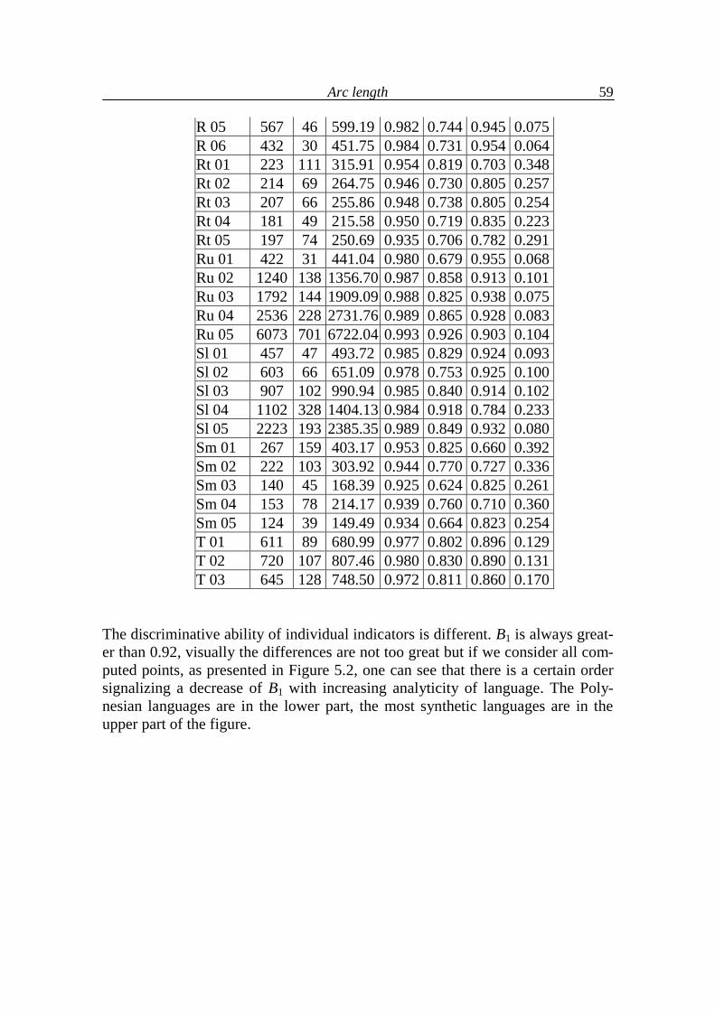
Arc length

59

R 05 567 46 599.19 0.982 0.744 0.945 0.075 R 06 432 30 451.75 0.984 0.731 0.954 0.064 Rt 01 223 111 315.91 0.954 0.819 0.703 0.348 Rt 02 214 69 264.75 0.946 0.730 0.805 0.257 Rt 03 207 66 255.86 0.948 0.738 0.805 0.254 Rt 04 181 49 215.58 0.950 0.719 0.835 0.223 Rt 05 197 74 250.69 0.935 0.706 0.782 0.291 Ru 01 422 31 441.04 0.980 0.679 0.955 0.068 Ru 02 1240 138 1356.70 0.987 0.858 0.913 0.101 Ru 03 1792 144 1909.09 0.988 0.825 0.938 0.075 Ru 04 2536 228 2731.76 0.989 0.865 0.928 0.083 Ru 05 6073 701 6722.04 0.993 0.926 0.903 0.104 Sl 01 457 47 493.72 0.985 0.829 0.924 0.093 Sl 02 603 66 651.09 0.978 0.753 0.925 0.100 Sl 03 907 102 990.94 0.985 0.840 0.914 0.102 Sl 04 1102 328 1404.13 0.984 0.918 0.784 0.233 Sl 05 2223 193 2385.35 0.989 0.849 0.932 0.080 Sm 01 267 159 403.17 0.953 0.825 0.660 0.392 Sm 02 222 103 303.92 0.944 0.770 0.727 0.336 Sm 03 140 45 168.39 0.925 0.624 0.825 0.261 Sm 04 153 78 214.17 0.939 0.760 0.710 0.360 Sm 05 124 39 149.49 0.934 0.664 0.823 0.254 T 01 611 89 680.99 0.977 0.802 0.896 0.129 T 02 720 107 807.46 0.980 0.830 0.890 0.131 T 03 645 128 748.50 0.972 0.811 0.860 0.170

The discriminative ability of individual indicators is different. B1 is always great-er than 0.92, visually the differences are not too great but if we consider all com-puted points, as presented in Figure 5.2, one can see that there is a certain order signalizing a decrease of B1 with increasing analyticity of language. The Poly-nesian languages are in the lower part, the most synthetic languages are in the upper part of the figure.

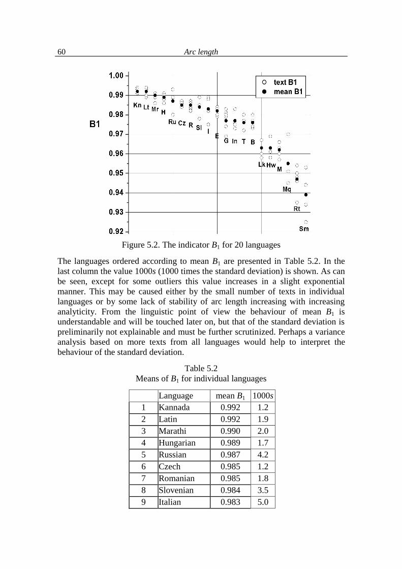
Arc length

60

Figure 5.2. The indicator B1 for 20 languages

The languages ordered according to mean B1 are presented in Table 5.2. In the last column the value 1000s (1000 times the standard deviation) is shown. As can be seen, except for some outliers this value increases in a slight exponential manner. This may be caused either by the small number of texts in individual languages or by some lack of stability of arc length increasing with increasing analyticity. From the linguistic point of view the behaviour of mean B1 is understandable and will be touched later on, but that of the standard deviation is preliminarily not explainable and must be further scrutinized. Perhaps a variance analysis based on more texts from all languages would help to interpret the behaviour of the standard deviation.

Table 5.2 Means of B1 for individual languages

Language mean B1 1000s 1 Kannada 0.992 1.2 2 Latin 0.992 1.9 3 Marathi 0.990 2.0 4 Hungarian 0.989 1.7 5 Russian 0.987 4.2 6 Czech 0.985 1.2 7 Romanian 0.985 1.8 8 Slovenian 0.984 3.5 9 Italian 0.983 5.0

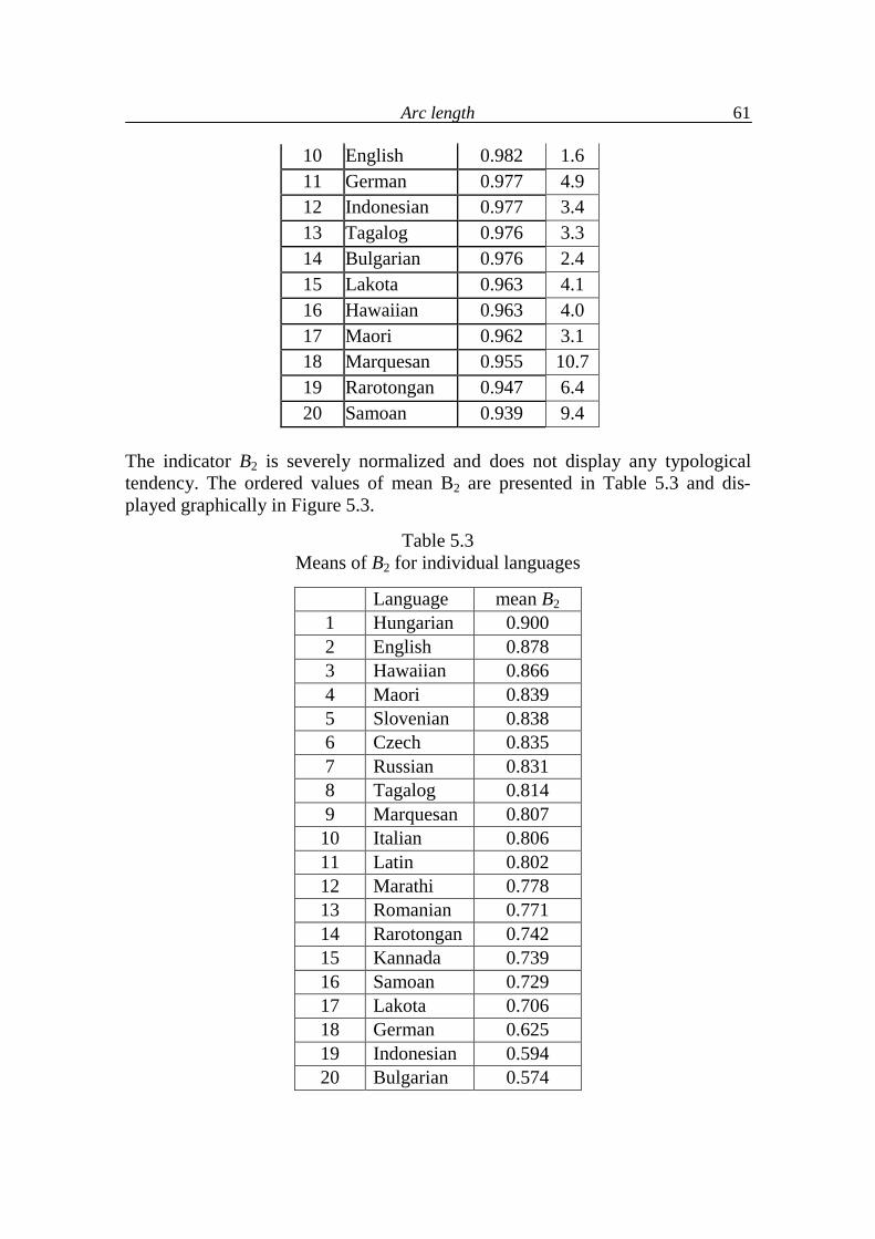
Arc length

61

10 English 0.982 1.6 11 German 0.977 4.9 12 Indonesian 0.977 3.4 13 Tagalog 0.976 3.3 14 Bulgarian 0.976 2.4 15 Lakota 0.963 4.1 16 Hawaiian 0.963 4.0 17 Maori 0.962 3.1 18 Marquesan 0.955 10.7 19 Rarotongan 0.947 6.4 20 Samoan 0.939 9.4

The indicator B2 is severely normalized and does not display any typological tendency. The ordered values of mean B2 are presented in Table 5.3 and dis-played graphically in Figure 5.3.

Table 5.3 Means of B2 for individual languages

Language mean B2

1 Hungarian 0.900 2 English 0.878 3 Hawaiian 0.866 4 Maori 0.839 5 Slovenian 0.838 6 Czech 0.835 7 Russian 0.831 8 Tagalog 0.814 9 Marquesan 0.807 10 Italian 0.806 11 Latin 0.802 12 Marathi 0.778 13 Romanian 0.771 14 Rarotongan 0.742 15 Kannada 0.739 16 Samoan 0.729 17 Lakota 0.706 18 German 0.625 19 Indonesian 0.594 20 Bulgarian 0.574

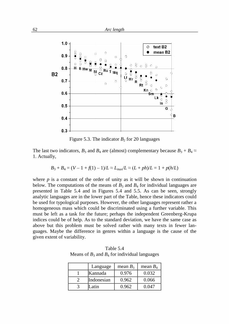
Arc length

62

Figure 5.3. The indicator B2 for 20 languages

The last two indicators, B3 and B4 are (almost) complementary because B3 + B4 ≈ 1. Actually,

B3 + B4 = (V – 1 + f(1) – 1)/L ≈ Lmax/L ≈ (L + ph)/L = 1 + p(h/L)

where p is a constant of the order of unity as it will be shown in continuation below. The computations of the means of B3 and B4 for individual languages are presented in Table 5.4 and in Figures 5.4 and 5.5. As can be seen, strongly analytic languages are in the lower part of the Table, hence these indicators could be used for typological purposes. However, the other languages represent rather a homogeneous mass which could be discriminated using a further variable. This must be left as a task for the future; perhaps the independent Greenberg-Krupa indices could be of help. As to the standard deviation, we have the same case as above but this problem must be solved rather with many texts in fewer lan-guages. Maybe the difference in genres within a language is the cause of the given extent of variability.

Table 5.4 Means of B3 and B4 for individual languages

Language mean B3 mean B4

1 Kannada 0.976 0.032 2 Indonesian 0.962 0.066 3 Latin 0.962 0.047

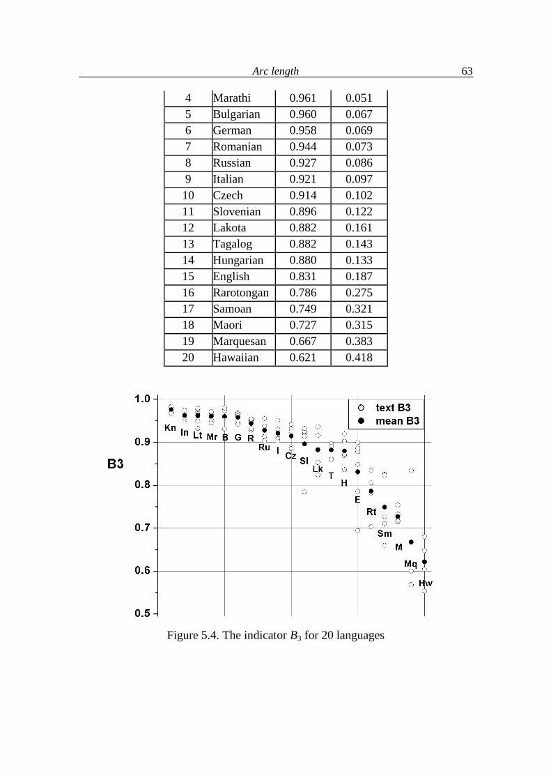
Arc length

63

4 Marathi 0.961 0.051 5 Bulgarian 0.960 0.067 6 German 0.958 0.069 7 Romanian 0.944 0.073 8 Russian 0.927 0.086 9 Italian 0.921 0.097

10 Czech 0.914 0.102 11 Slovenian 0.896 0.122 12 Lakota 0.882 0.161 13 Tagalog 0.882 0.143 14 Hungarian 0.880 0.133 15 English 0.831 0.187 16 Rarotongan 0.786 0.275 17 Samoan 0.749 0.321 18 Maori 0.727 0.315 19 Marquesan 0.667 0.383 20 Hawaiian 0.621 0.418

Figure 5.4. The indicator B3 for 20 languages

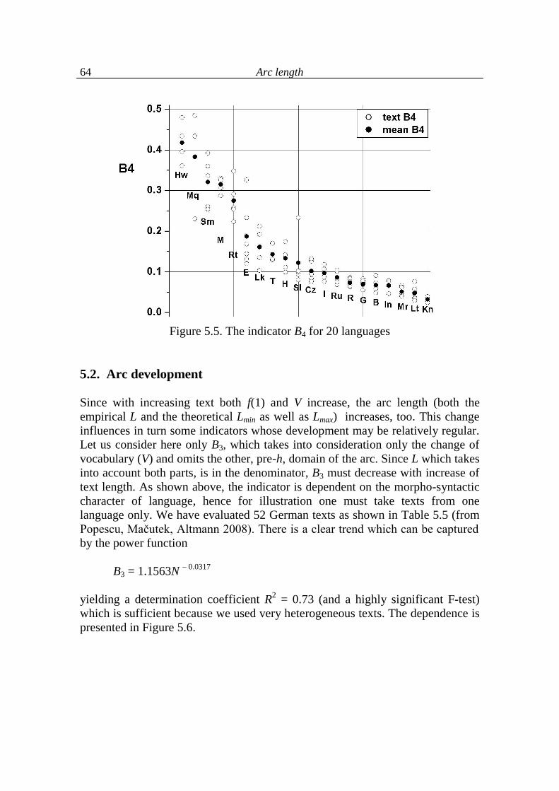
Arc length

64

Figure 5.5. The indicator B4 for 20 languages

5.2. Arc development Since with increasing text both f(1) and V increase, the arc length (both the empirical L and the theoretical Lmin as well as Lmax) increases, too. This change influences in turn some indicators whose development may be relatively regular. Let us consider here only B3, which takes into consideration only the change of vocabulary (V) and omits the other, pre-h, domain of the arc. Since L which takes into account both parts, is in the denominator, B3 must decrease with increase of text length. As shown above, the indicator is dependent on the morpho-syntactic character of language, hence for illustration one must take texts from one language only. We have evaluated 52 German texts as shown in Table 5.5 (from Popescu, Mačutek, Altmann 2008). There is a clear trend which can be captured by the power function B3 = 1.1563N – 0.0317

yielding a determination coefficient R2 = 0.73 (and a highly significant F-test) which is sufficient because we used very heterogeneous texts. The dependence is presented in Figure 5.6.

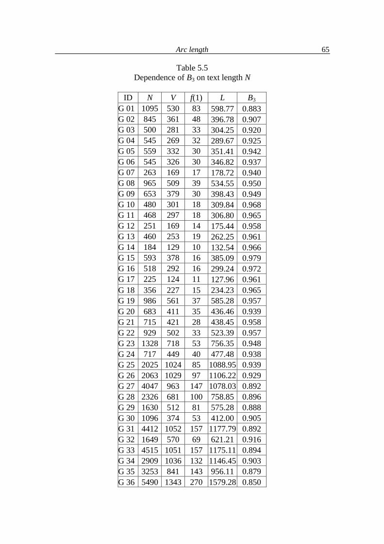
Arc length

65

Table 5.5 Dependence of B3 on text length N

ID N V f(1) L B3

G 01 1095 530 83 598.77 0.883 G 02 845 361 48 396.78 0.907 G 03 500 281 33 304.25 0.920 G 04 545 269 32 289.67 0.925 G 05 559 332 30 351.41 0.942 G 06 545 326 30 346.82 0.937 G 07 263 169 17 178.72 0.940 G 08 965 509 39 534.55 0.950 G 09 653 379 30 398.43 0.949 G 10 480 301 18 309.84 0.968 G 11 468 297 18 306.80 0.965 G 12 251 169 14 175.44 0.958 G 13 460 253 19 262.25 0.961 G 14 184 129 10 132.54 0.966 G 15 593 378 16 385.09 0.979 G 16 518 292 16 299.24 0.972 G 17 225 124 11 127.96 0.961 G 18 356 227 15 234.23 0.965 G 19 986 561 37 585.28 0.957 G 20 683 411 35 436.46 0.939 G 21 715 421 28 438.45 0.958 G 22 929 502 33 523.39 0.957 G 23 1328 718 53 756.35 0.948 G 24 717 449 40 477.48 0.938 G 25 2025 1024 85 1088.95 0.939 G 26 2063 1029 97 1106.22 0.929 G 27 4047 963 147 1078.03 0.892 G 28 2326 681 100 758.85 0.896 G 29 1630 512 81 575.28 0.888 G 30 1096 374 53 412.00 0.905 G 31 4412 1052 157 1177.79 0.892 G 32 1649 570 69 621.21 0.916 G 33 4515 1051 157 1175.11 0.894 G 34 2909 1036 132 1146.45 0.903 G 35 3253 841 143 956.11 0.879 G 36 5490 1343 270 1579.28 0.850

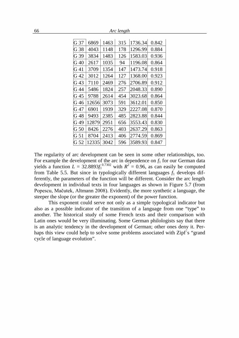
Arc length

66

G 37 6869 1463 315 1736.34 0.842 G 38 4043 1148 178 1296.99 0.884 G 39 3834 1483 126 1583.03 0.936 G 40 2617 1035 94 1196.08 0.864 G 41 3709 1354 147 1473.74 0.918 G 42 3012 1264 127 1368.00 0.923 G 43 7110 2469 276 2706.89 0.912 G 44 5486 1824 257 2048.33 0.890 G 45 9788 2614 454 3023.68 0.864 G 46 12656 3073 591 3612.01 0.850 G 47 6901 1939 329 2227.08 0.870 G 48 9493 2385 485 2823.88 0.844 G 49 12879 2951 656 3553.43 0.830 G 50 8426 2276 403 2637.29 0.863 G 51 8704 2413 406 2774.59 0.869 G 52 12335 3042 596 3589.93 0.847

The regularity of arc development can be seen in some other relationships, too. For example the development of the arc in dependence on f1 for our German data yields a function L = 32.8893f1

0.7302 with R2 = 0.96, as can easily be computed from Table 5.5. But since in typologically different languages f1 develops dif-ferently, the parameters of the function will be different. Consider the arc length development in individual texts in four languages as shown in Figure 5.7 (from Popescu, Mačutek, Altmann 2008). Evidently, the more synthetic a language, the steeper the slope (or the greater the exponent) of the power function. This exponent could serve not only as a simple typological indicator but also as a possible indicator of the transition of a language from one “type” to another. The historical study of some French texts and their comparison with Latin ones would be very illuminating. Some German philologists say that there is an analytic tendency in the development of German; other ones deny it. Per-haps this view could help to solve some problems associated with Zipf´s “grand cycle of language evolution”.

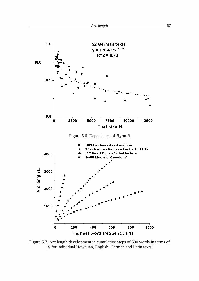
Arc length

67

Figure 5.6. Dependence of B3 on N

Figure 5.7. Arc length development in cumulative steps of 500 words in terms of

f1 for individual Hawaiian, English, German and Latin texts

Arc length

68

5.3. Arc length as a function of text indicators In all above dependences some empirical constants appeared whose linguistic interpretation was not possible. As a matter of fact, capturing a dependence in this way is a play with the ceteris paribus conditions. The constants indicate that there is still something else having a constant influence on the dependent variable through the independent variable. In this sense, for instance, Table 5.18 with word form indicators of 100 texts, selected from 20 languages, demonstrates empirically the following relationship (5.24) L = Lmax – p(h – 1) where p is a constant of the order of unity, telling us that the difference between the arc length L and its maximum possible value Lmax is always of the order of h. As needed, in the extreme case of h = 1 we have L = Lmax. The relationship (5.24) seems to be a basic textual property involving the h-point and has previously been verified in a slightly simplified form, as (5.25) L = V + f(1) – ch , where c is also a constant of the order of unity (Popescu, Mačutek, Altmann 2008). As a matter of fact, Eq. (5.24) is a relationship between the arc length L, both V and f1 (through Lmax) as well as the h-point, all of which developing regularly with increasing N.

In the following applications we shall generalize the relationship (5.24) in order to compute the coefficient

(5.26) max

1L Lp

h

for any rank-frequency distribution f = f(r), where (5.27) Lmax = (R – 1) + f(1) – f(R) is the ideal maximum arc length, rmax = R the maximum rank, f(1) the maximum frequency, and f(R) the minimum frequency. For the sake of comparison we shall generalize also the equation (5.25) in the form (5.28) L = R + f(1) – f(R) + 1 – ch from which we get the coefficient

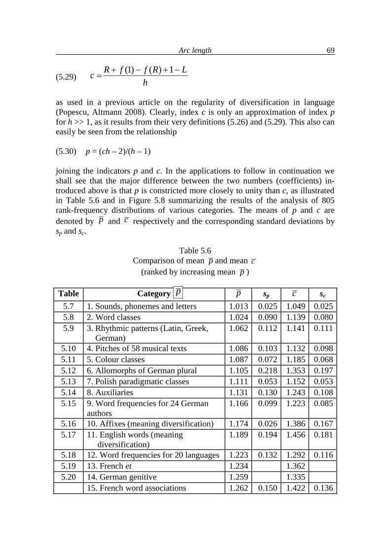
Arc length

69

(5.29) (1) ( ) 1R f f R Lc

h

as used in a previous article on the regularity of diversification in language (Popescu, Altmann 2008). Clearly, index c is only an approximation of index p for h >> 1, as it results from their very definitions (5.26) and (5.29). This also can easily be seen from the relationship (5.30) p = (ch – 2)/(h – 1) joining the indicators p and c. In the applications to follow in continuation we shall see that the major difference between the two numbers (coefficients) in-troduced above is that p is constricted more closely to unity than c, as illustrated in Table 5.6 and in Figure 5.8 summarizing the results of the analysis of 805 rank-frequency distributions of various categories. The means of p and c are denoted by p and c respectively and the corresponding standard deviations by sp and sc.

Table 5.6

Comparison of mean p and mean c (ranked by increasing mean p )

Table Category p sp c sc

5.7 1. Sounds, phonemes and letters 1.013 0.025 1.049 0.025 5.8 2. Word classes 1.024 0.090 1.139 0.080 5.9 3. Rhythmic patterns (Latin, Greek,

German) 1.062 0.112 1.141 0.111

5.10 4. Pitches of 58 musical texts 1.086 0.103 1.132 0.098 5.11 5. Colour classes 1.087 0.072 1.185 0.068 5.12 6. Allomorphs of German plural 1.105 0.218 1.353 0.197 5.13 7. Polish paradigmatic classes 1.111 0.053 1.152 0.053 5.14 8. Auxiliaries 1.131 0.130 1.243 0.108 5.15 9. Word frequencies for 24 German

authors 1.166 0.099 1.223 0.085

5.16 10. Affixes (meaning diversification) 1.174 0.026 1.386 0.167 5.17 11. English words (meaning

diversification) 1.189 0.194 1.456 0.181

5.18 12. Word frequencies for 20 languages 1.223 0.132 1.292 0.116 5.19 13. French et 1.234 1.362 5.20 14. German genitive 1.259 1.335

15. French word associations 1.262 0.150 1.422 0.136

p

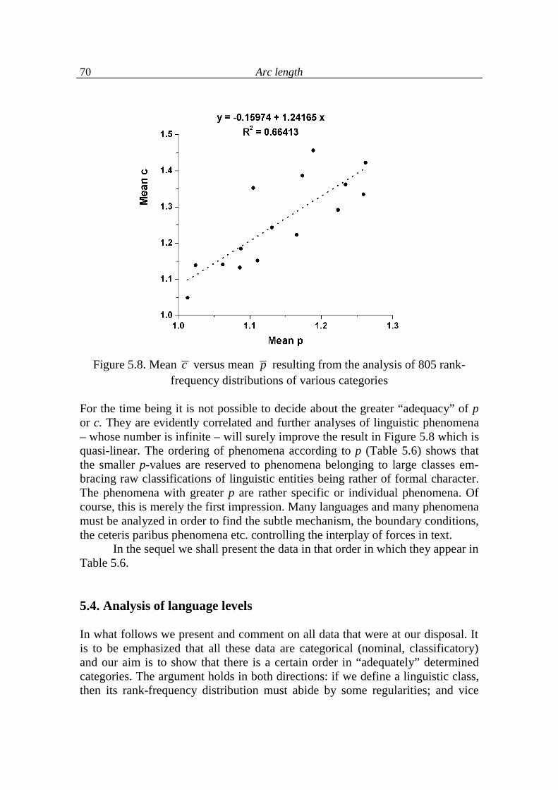
Arc length

70

Figure 5.8. Mean c versus mean p resulting from the analysis of 805 rank-

frequency distributions of various categories For the time being it is not possible to decide about the greater “adequacy” of p or c. They are evidently correlated and further analyses of linguistic phenomena – whose number is infinite – will surely improve the result in Figure 5.8 which is quasi-linear. The ordering of phenomena according to p (Table 5.6) shows that the smaller p-values are reserved to phenomena belonging to large classes em-bracing raw classifications of linguistic entities being rather of formal character. The phenomena with greater p are rather specific or individual phenomena. Of course, this is merely the first impression. Many languages and many phenomena must be analyzed in order to find the subtle mechanism, the boundary conditions, the ceteris paribus phenomena etc. controlling the interplay of forces in text. In the sequel we shall present the data in that order in which they appear in Table 5.6.

5.4. Analysis of language levels In what follows we present and comment on all data that were at our disposal. It is to be emphasized that all these data are categorical (nominal, classificatory) and our aim is to show that there is a certain order in “adequately” determined categories. The argument holds in both directions: if we define a linguistic class, then its rank-frequency distribution must abide by some regularities; and vice

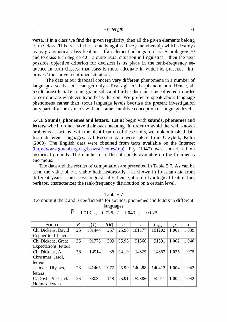
Arc length

71

versa, if in a class we find the given regularity, then all the given elements belong to the class. This is a kind of remedy against fuzzy membership which destroys many grammatical classifications. If an element belongs to class A in degree 70 and to class B in degree 40 – a quite usual situation in linguistics – then the next possible objective criterion for decision is its place in the rank-frequency se-quence in both classes: that class is more adequate in which its presence “im-proves” the above mentioned situation. The data at our disposal concern very different phenomena in a number of languages, so that one can get only a first sight of the phenomenon. Hence, all results must be taken cum grano salis and further data must be collected in order to corroborate whatever hypothesis thereon. We prefer to speak about language phenomena rather than about language levels because the present investigation only partially corresponds with our rather intuitive conception of language level. 5.4.1. Sounds, phonemes and letters. Let us begin with sounds, phonemes and letters which do not have their own meaning. In order to avoid the well known problems associated with the identification of these units, we took published data from different languages. All Russian data were taken from Grzybek, Kelih (2003). The English data were obtained from texts available on the Internet (http://www.gutenberg.org/browse/scores/top). Fry (1947) was considered on historical grounds. The number of different counts available on the Internet is enormous.

The data and the results of computation are presented in Table 5.7. As can be seen, the value of c is stable both historically – as shown in Russian data from different years – and cross-linguistically, hence, it is no typological feature but, perhaps, characterizes the rank-frequency distribution on a certain level.

Table 5.7

Computing the c and p coefficients for sounds, phonemes and letters in different languages

p = 1.013, sp = 0.025, c = 1.049, sc = 0.025

Source R f(1) f(R) h L Lmax p c Ch. Dickens, David Copperfield, letters

26 181444 267 25.98 181177 181202 1.001 1.039

Ch. Dickens, Great Expectations, letters

26 91775 209 25.95 91566 91591 1.002 1.040

Ch. Dickens, A Christmas Carol, letters

26 14914 86 24.19 14829 14853 1.035 1.075

J. Joyce, Ulysses, letters

26 141465 1077 25.90 140388 140413 1.004 1.042

C. Doyle, Sherlock Holmes, letters

26 53034 148 25.91 52886 52911 1.004 1.042

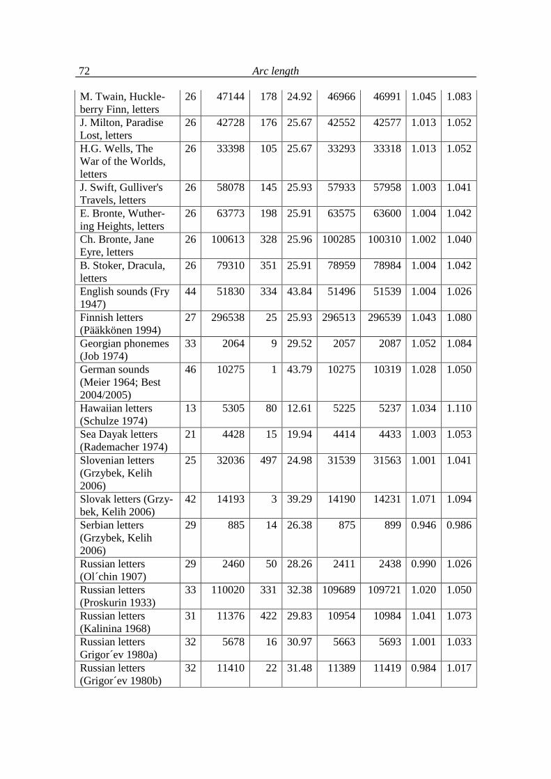
Arc length

72

M. Twain, Huckle-berry Finn, letters

26 47144 178 24.92 46966 46991 1.045 1.083

J. Milton, Paradise Lost, letters

26 42728 176 25.67 42552 42577 1.013 1.052

H.G. Wells, The War of the Worlds, letters

26 33398 105 25.67 33293 33318 1.013 1.052

J. Swift, Gulliver's Travels, letters

26 58078 145 25.93 57933 57958 1.003 1.041

E. Bronte, Wuther-ing Heights, letters

26 63773 198 25.91 63575 63600 1.004 1.042

Ch. Bronte, Jane Eyre, letters

26 100613 328 25.96 100285 100310 1.002 1.040

B. Stoker, Dracula, letters

26 79310 351 25.91 78959 78984 1.004 1.042

English sounds (Fry 1947)

44 51830 334 43.84 51496 51539 1.004 1.026

Finnish letters (Pääkkönen 1994)

27 296538 25 25.93 296513 296539 1.043 1.080

Georgian phonemes (Job 1974)

33 2064 9 29.52 2057 2087 1.052 1.084

German sounds (Meier 1964; Best 2004/2005)

46 10275 1 43.79 10275 10319 1.028 1.050

Hawaiian letters (Schulze 1974)

13 5305 80 12.61 5225 5237 1.034 1.110

Sea Dayak letters (Rademacher 1974)

21 4428 15 19.94 4414 4433 1.003 1.053

Slovenian letters (Grzybek, Kelih 2006)

25 32036 497 24.98 31539 31563 1.001 1.041

Slovak letters (Grzy- bek, Kelih 2006)

42 14193 3 39.29 14190 14231 1.071 1.094

Serbian letters (Grzybek, Kelih 2006)

29 885 14 26.38 875 899 0.946 0.986

Russian letters (Ol´chin 1907)

29 2460 50 28.26 2411 2438 0.990 1.026

Russian letters (Proskurin 1933)

33 110020 331 32.38 109689 109721 1.020 1.050

Russian letters (Kalinina 1968)

31 11376 422 29.83 10954 10984 1.041 1.073

Russian letters Grigor´ev 1980a)

32 5678 16 30.97 5663 5693 1.001 1.033

Russian letters (Grigor´ev 1980b)

32 11410 22 31.48 11389 11419 0.984 1.017

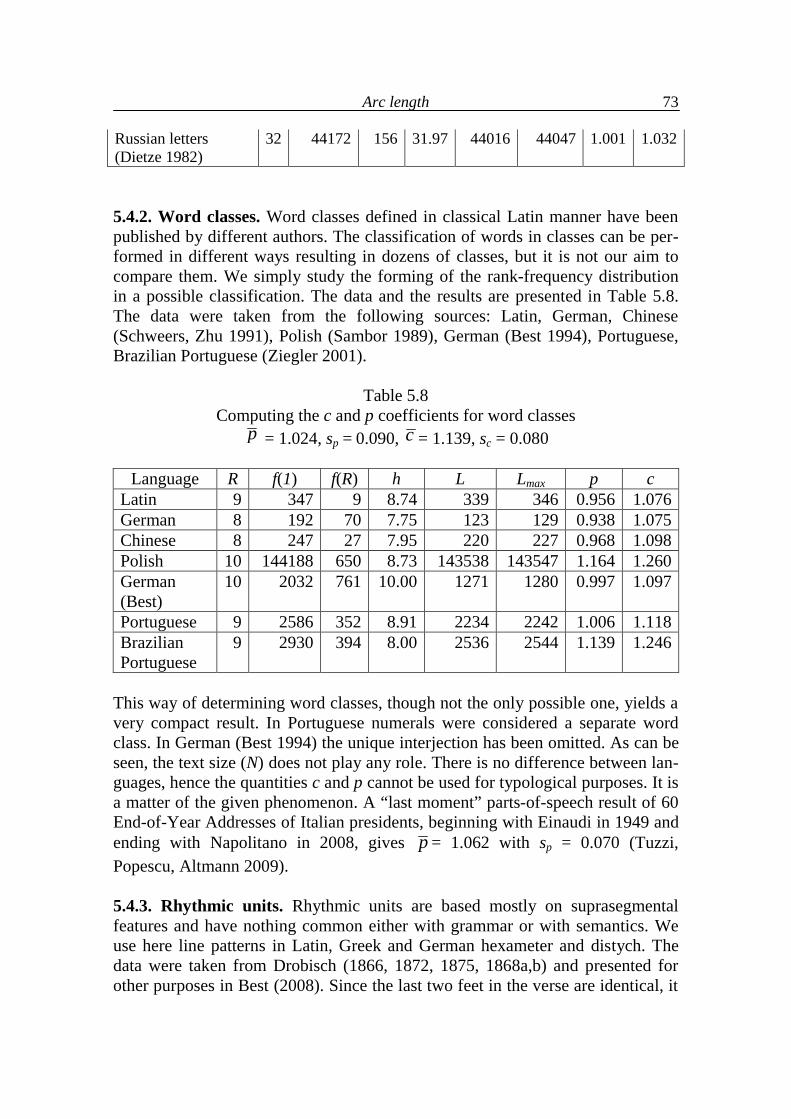
Arc length

73

Russian letters (Dietze 1982)

32 44172 156 31.97 44016 44047 1.001 1.032

5.4.2. Word classes. Word classes defined in classical Latin manner have been published by different authors. The classification of words in classes can be per-formed in different ways resulting in dozens of classes, but it is not our aim to compare them. We simply study the forming of the rank-frequency distribution in a possible classification. The data and the results are presented in Table 5.8. The data were taken from the following sources: Latin, German, Chinese (Schweers, Zhu 1991), Polish (Sambor 1989), German (Best 1994), Portuguese, Brazilian Portuguese (Ziegler 2001).

Table 5.8 Computing the c and p coefficients for word classes

p = 1.024, sp = 0.090, c = 1.139, sc = 0.080

Language R f(1) f(R) h L Lmax p c Latin 9 347 9 8.74 339 346 0.956 1.076 German 8 192 70 7.75 123 129 0.938 1.075 Chinese 8 247 27 7.95 220 227 0.968 1.098 Polish 10 144188 650 8.73 143538 143547 1.164 1.260 German (Best)

10 2032 761 10.00 1271 1280 0.997 1.097

Portuguese 9 2586 352 8.91 2234 2242 1.006 1.118 Brazilian Portuguese

9 2930 394 8.00 2536 2544 1.139 1.246

This way of determining word classes, though not the only possible one, yields a very compact result. In Portuguese numerals were considered a separate word class. In German (Best 1994) the unique interjection has been omitted. As can be seen, the text size (N) does not play any role. There is no difference between lan-guages, hence the quantities c and p cannot be used for typological purposes. It is a matter of the given phenomenon. A “last moment” parts-of-speech result of 60 End-of-Year Addresses of Italian presidents, beginning with Einaudi in 1949 and ending with Napolitano in 2008, gives p = 1.062 with sp = 0.070 (Tuzzi, Popescu, Altmann 2009). 5.4.3. Rhythmic units. Rhythmic units are based mostly on suprasegmental features and have nothing common either with grammar or with semantics. We use here line patterns in Latin, Greek and German hexameter and distych. The data were taken from Drobisch (1866, 1872, 1875, 1868a,b) and presented for other purposes in Best (2008). Since the last two feet in the verse are identical, it

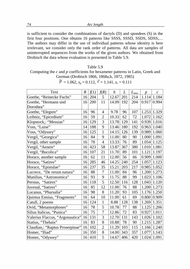
Arc length

74

is sufficient to consider the combinations of dactyls (D) and spondees (S) in the first four positions. One obtains 16 patterns like SSSS, SSSD, SSDS, SDSS,… The authors may differ in the use of individual patterns whose identity is here irrelevant, we consider only the rank order of patterns. All data are samples of uninterrupted sequences from the works of the given authors. We obtained from Drobisch the data whose evaluation is presented in Table 5.9.

Table 5.9 Computing the c and p coefficients for hexameter patterns in Latin, Greek and

German (Drobisch 1866, 1868a,b, 1872, 1985) p = 1.062, sp = 0.112, c = 1.141, sc = 0.111

Text R f(1) f(R) h L Lmax p c

Goethe, “Reinecke Fuchs” 16 204 5 12.67 201 214 1.114 1.184 Goethe, “Hermann und Dorothea”

16 200 11 14.09 192 204 0.917 0.994

Goethe, “Elegien” 16 96 4 9.78 96 107 1.253 1.329 Leibniz, “Epicedium” 16 59 2 10.33 62 72 1.072 1.162 Klopstock,: “Messias” 16 129 3 13.78 129 141 0.939 1.016 Voss, “Luise” 14 188 9 13.46 180 192 0.963 1.040 Voss, “Odyssey” 16 125 1 14.15 126 139 0.989 1.060 Vergil, “Georgica” 16 84 9 11.00 80 90 1.000 1.091 Vergil, other sample 16 78 4 13.33 76 89 1.054 1.125 Vergil, “Aeneis“ 16 423 58 13.87 367 380 1.010 1.081 Vergil, “Bucolica” 16 107 21 11.70 89 101 1.121 1.197 Horace, another sample 16 62 11 12.00 56 66 0.909 1.000 Horace, “Satires” 16 285 46 14.25 240 254 1.057 1.123 Horace, “Epistulae” 16 237 35 15.21 203 217 0.985 1.052 Lucrece, “De rerum natura” 16 88 7 11.00 84 96 1.200 1.273 Manilius, “Astronomica” 16 93 9 11.75 88 99 1.023 1.106 Persius, “Satires” 16 118 5 12.50 116 128 1.043 1.120 Juvenal, “Satires” 16 85 12 11.00 76 88 1.200 1.273 Lucanus, “Pharsalia” 16 98 8 11.20 93 105 1.176 1.250 Quintus Ennius, “Fragments” 16 64 10 11.00 61 69 0.800 0.909 Catull, 2 poems 16 124 1 8.88 128 138 1.269 1.351 Ovid, “Metamorphoses” 16 78 5 10.78 77 88 1.125 1.206 Silius Italicus, “Punica” 16 75 7 12.86 72 83 0.927 1.011 Valerius Flaccus, “Argonautica” 16 131 3 12.70 131 143 1.026 1.102 Statius, “Thebais” 16 83 8 10.88 78 90 1.215 1.287 Claudian,: “Raptus Proserpinae” 16 102 2 11.29 103 115 1.166 1.240 Homer, “Iliad” 16 350 8 14.00 343 357 1.077 1.143 Homer, “Odyssey” 16 410 5 14.67 406 420 1.024 1.091

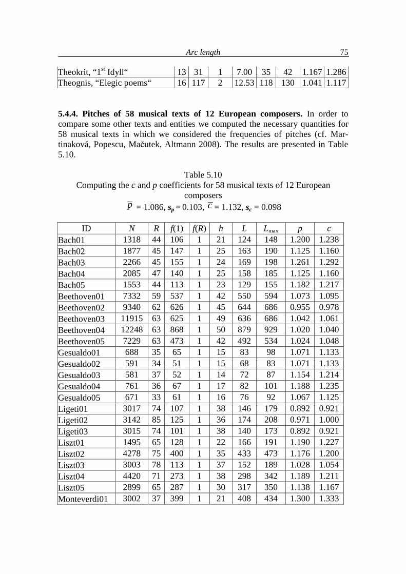
Arc length

75

Theokrit, “1st Idyll“ 13 31 1 7.00 35 42 1.167 1.286 Theognis, “Elegic poems“ 16 117 2 12.53 118 130 1.041 1.117

5.4.4. Pitches of 58 musical texts of 12 European composers. In order to compare some other texts and entities we computed the necessary quantities for 58 musical texts in which we considered the frequencies of pitches (cf. Mar-tinaková, Popescu, Mačutek, Altmann 2008). The results are presented in Table 5.10.

Table 5.10 Computing the c and p coefficients for 58 musical texts of 12 European

composers p = 1.086, sp = 0.103, c = 1.132, sc = 0.098

ID N R f(1) f(R) h L Lmax p c

Bach01 1318 44 106 1 21 124 148 1.200 1.238 Bach02 1877 45 147 1 25 163 190 1.125 1.160 Bach03 2266 45 155 1 24 169 198 1.261 1.292 Bach04 2085 47 140 1 25 158 185 1.125 1.160 Bach05 1553 44 113 1 23 129 155 1.182 1.217 Beethoven01 7332 59 537 1 42 550 594 1.073 1.095 Beethoven02 9340 62 626 1 45 644 686 0.955 0.978 Beethoven03 11915 63 625 1 49 636 686 1.042 1.061 Beethoven04 12248 63 868 1 50 879 929 1.020 1.040 Beethoven05 7229 63 473 1 42 492 534 1.024 1.048 Gesualdo01 688 35 65 1 15 83 98 1.071 1.133 Gesualdo02 591 34 51 1 15 68 83 1.071 1.133 Gesualdo03 581 37 52 1 14 72 87 1.154 1.214 Gesualdo04 761 36 67 1 17 82 101 1.188 1.235 Gesualdo05 671 33 61 1 16 76 92 1.067 1.125 Ligeti01 3017 74 107 1 38 146 179 0.892 0.921 Ligeti02 3142 85 125 1 36 174 208 0.971 1.000 Ligeti03 3015 74 101 1 38 140 173 0.892 0.921 Liszt01 1495 65 128 1 22 166 191 1.190 1.227 Liszt02 4278 75 400 1 35 433 473 1.176 1.200 Liszt03 3003 78 113 1 37 152 189 1.028 1.054 Liszt04 4420 71 273 1 38 298 342 1.189 1.211 Liszt05 2899 65 287 1 30 317 350 1.138 1.167 Monteverdi01 3002 37 399 1 21 408 434 1.300 1.333

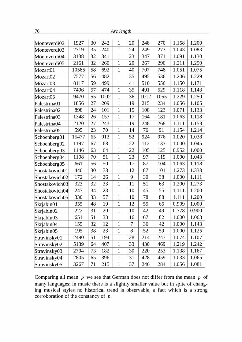
Arc length

76

Monteverdi02 1927 30 242 1 20 248 270 1.158 1.200 Monteverdi03 2719 35 240 1 24 249 273 1.043 1.083 Monteverdi04 3138 32 341 1 23 347 371 1.091 1.130 Monteverdi05 2161 32 260 1 20 267 290 1.211 1.250 Mozart01 10585 58 692 1 40 707 748 1.051 1.075 Mozart02 7577 56 482 1 35 495 536 1.206 1.229 Mozart03 8117 59 499 1 41 510 556 1.150 1.171 Mozart04 7496 57 474 1 35 491 529 1.118 1.143 Mozart05 9470 55 1002 1 36 1012 1055 1.229 1.250 Palestrina01 1856 27 209 1 19 215 234 1.056 1.105 Palestrina02 898 24 101 1 15 108 123 1.071 1.133 Palestrina03 1348 26 157 1 17 164 181 1.063 1.118 Palestrina04 2120 27 243 1 19 248 268 1.111 1.158 Palestrina05 595 23 70 1 14 76 91 1.154 1.214 Schoenberg01 15477 65 913 1 52 924 976 1.020 1.038 Schoenberg02 1197 67 68 1 22 112 133 1.000 1.045 Schoenberg03 1146 63 64 1 22 105 125 0.952 1.000 Schoenberg04 1108 70 51 1 23 97 119 1.000 1.043 Schoenberg05 661 56 50 1 17 87 104 1.063 1.118 Shostakovich01 440 30 73 1 12 87 101 1.273 1.333 Shostakovich02 172 14 26 1 9 30 38 1.000 1.111 Shostakovich03 323 32 33 1 11 51 63 1.200 1.273 Shostakovich04 247 34 23 1 10 45 55 1.111 1.200 Shostakovich05 330 33 57 1 10 78 88 1.111 1.200 Skrjabin01 355 48 19 1 12 55 65 0.909 1.000 Skrjabin02 222 31 20 1 10 42 49 0.778 0.900 Skrjabin03 651 51 33 1 16 67 82 1.000 1.063 Skrjabin04 155 32 12 1 7 36 42 1.000 1.143 Skrjabin05 195 38 23 1 8 52 59 1.000 1.125 Stravinsky01 2490 51 194 1 28 214 243 1.074 1.107 Stravinsky02 5139 64 407 1 33 430 469 1.219 1.242 Stravinsky03 2794 73 182 1 30 220 253 1.138 1.167 Stravinsky04 2805 65 396 1 31 428 459 1.033 1.065 Stravinsky05 3267 71 215 1 37 246 284 1.056 1.081 Comparing all mean p we see that German does not differ from the mean p of many languages; in music there is a slightly smaller value but in spite of chang-ing musical styles no historical trend is observable, a fact which is a strong corroboration of the constancy of p.

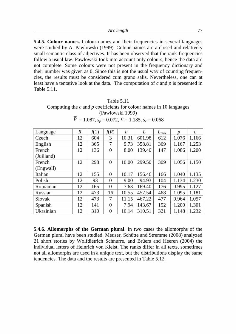
Arc length

77

5.4.5. Colour names. Colour names and their frequencies in several languages were studied by A. Pawlowski (1999). Colour names are a closed and relatively small semantic class of adjectives. It has been observed that the rank-frequencies follow a usual law. Pawlowski took into account only colours, hence the data are not complete. Some colours were not present in the frequency dictionary and their number was given as 0. Since this is not the usual way of counting frequen-cies, the results must be considered cum grano salis. Nevertheless, one can at least have a tentative look at the data. The computation of c and p is presented in Table 5.11.

Table 5.11

Computing the c and p coefficients for colour names in 10 languages (Pawlowski 1999)

p = 1.087, sp = 0.072, c = 1.185, sc = 0.068 Language R f(1) f(R) h L Lmax p c Czech 12 604 3 10.31 601.98 612 1.076 1.166 English 12 365 7 9.73 358.81 369 1.167 1.253 French (Juilland)

12 136 0 8.00 139.40 147 1.086 1.200

French (Engwall)

12 298 0 10.00 299.50 309 1.056 1.150

Italian 12 155 0 10.17 156.46 166 1.040 1.135 Polish 12 93 0 9.00 94.93 104 1.134 1.230 Romanian 12 165 0 7.63 169.40 176 0.995 1.127 Russian 12 473 16 10.55 457.54 468 1.095 1.181 Slovak 12 473 7 11.15 467.22 477 0.964 1.057 Spanish 12 141 0 7.94 143.67 152 1.200 1.301 Ukrainian 12 310 0 10.14 310.51 321 1.148 1.232

5.4.6. Allomorphs of the German plural. In two cases the allomorphs of the German plural have been studied. Meuser, Schütte and Stremme (2008) analyzed 21 short stories by Wolfdietrich Schnurre, and Brüers and Heeren (2004) the individual letters of Heinrich von Kleist. The ranks differ in all texts, sometimes not all allomorphs are used in a unique text, but the distributions display the same tendencies. The data and the results are presented in Table 5.12.

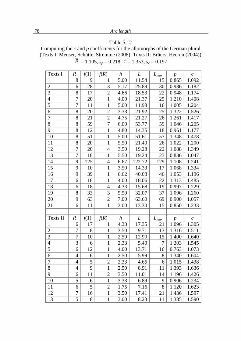
Arc length

78

Table 5.12 Computing the c and p coefficients for the allomorphs of the German plural (Texts I: Meuser, Schütte, Stremme (2008); Texts II: Brüers, Heeren (2004))

p = 1.105, sp = 0.218, c = 1.353, sc = 0.197

Texts I R f(1) f(R) h L Lmax p c 1 8 9 1 5.00 11.54 15 0.865 1.092 2 6 28 3 5.17 25.89 30 0.986 1.182 3 8 17 2 4.66 18.53 22 0.948 1.174 4 7 20 1 4.00 21.37 25 1.210 1.408 5 7 11 1 5.00 11.98 16 1.005 1.204 6 8 20 2 3.33 21.92 25 1.322 1.526 7 8 21 2 4.75 21.27 26 1.261 1.417 8 8 59 7 6.00 53.77 59 1.046 1.205 9 8 12 1 4.80 14.35 18 0.961 1.177 10 8 51 1 5.00 51.61 57 1.348 1.478 11 8 20 1 5.50 21.40 26 1.022 1.200 12 7 20 4 3.50 19.28 22 1.088 1.349 13 7 18 1 5.50 19.24 23 0.836 1.047 14 9 125 4 6.67 122.72 129 1.108 1.241 15 9 10 1 3.50 14.33 17 1.068 1.334 16 9 39 1 6.62 40.08 46 1.053 1.196 17 6 18 1 4.00 18.06 22 1.313 1.485 18 6 18 4 4.33 15.68 19 0.997 1.229 19 8 33 3 5.50 32.07 37 1.096 1.260 20 9 63 2 7.00 63.60 69 0.900 1.057 21 6 11 1 3.00 13.30 15 0.850 1.233 Texts II R f(1) f(R) h L Lmax p c 1 6 17 1 4.33 17.35 21 1.096 1.305 2 7 8 1 3.50 9.71 13 1.316 1.511 3 7 10 1 2.50 12.90 15 1.400 1.640 4 3 6 1 2.33 5.40 7 1.203 1.545 5 6 12 1 4.00 13.71 16 0.763 1.073 6 4 6 1 2.50 5.99 8 1.340 1.604 7 4 5 2 2.33 4.65 6 1.015 1.438 8 4 9 1 2.50 8.91 11 1.393 1.636 9 6 11 2 3.50 11.01 14 1.196 1.426 10 5 6 1 3.33 6.89 9 0.906 1.234 11 6 5 2 1.75 7.16 8 1.120 1.623 12 7 16 1 3.50 17.41 21 1.436 1.597 13 5 8 1 3.00 8.23 11 1.385 1.590

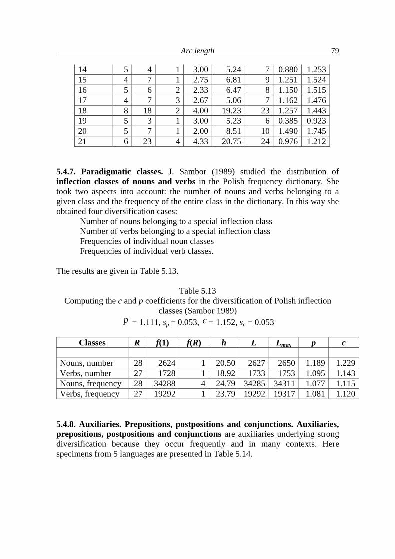
Arc length

79

14 5 4 1 3.00 5.24 7 0.880 1.253 15 4 7 1 2.75 6.81 9 1.251 1.524 16 5 6 2 2.33 6.47 8 1.150 1.515 17 4 7 3 2.67 5.06 7 1.162 1.476 18 8 18 2 4.00 19.23 23 1.257 1.443 19 5 3 1 3.00 5.23 6 0.385 0.923 20 5 7 1 2.00 8.51 10 1.490 1.745 21 6 23 4 4.33 20.75 24 0.976 1.212

5.4.7. Paradigmatic classes. J. Sambor (1989) studied the distribution of inflection classes of nouns and verbs in the Polish frequency dictionary. She took two aspects into account: the number of nouns and verbs belonging to a given class and the frequency of the entire class in the dictionary. In this way she obtained four diversification cases: Number of nouns belonging to a special inflection class Number of verbs belonging to a special inflection class Frequencies of individual noun classes Frequencies of individual verb classes. The results are given in Table 5.13.

Table 5.13 Computing the c and p coefficients for the diversification of Polish inflection

classes (Sambor 1989) p = 1.111, sp = 0.053, c = 1.152, sc = 0.053

Classes R f(1) f(R) h L Lmax p c

Nouns, number 28 2624 1 20.50 2627 2650 1.189 1.229 Verbs, number 27 1728 1 18.92 1733 1753 1.095 1.143 Nouns, frequency 28 34288 4 24.79 34285 34311 1.077 1.115 Verbs, frequency 27 19292 1 23.79 19292 19317 1.081 1.120

5.4.8. Auxiliaries. Prepositions, postpositions and conjunctions. Auxiliaries, prepositions, postpositions and conjunctions are auxiliaries underlying strong diversification because they occur frequently and in many contexts. Here specimens from 5 languages are presented in Table 5.14.

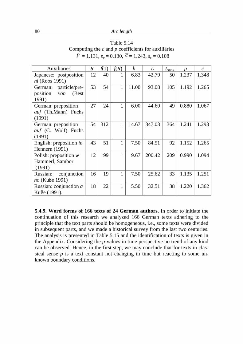
Arc length

80

Table 5.14 Computing the c and p coefficients for auxiliaries

p = 1.131, sp = 0.130, c = 1.243, sc = 0.108

Auxiliaries R f(1) f(R) h L Lmax p c Japanese: postposition ni (Roos 1991)

12 40 1 6.83 42.79 50 1.237 1.348

German: particle/pre-position von (Best 1991)

53 54 1 11.00 93.08 105 1.192 1.265

German: preposition auf (Th.Mann) Fuchs (1991)

27 24 1 6.00 44.60 49 0.880 1.067

German: preposition auf (C. Wolf) Fuchs (1991)

54 312 1 14.67 347.03 364 1.241 1.293

English: preposition in Hennern (1991)

43 51 1 7.50 84.51 92 1.152 1.265

Polish: preposition w Hammerl, Sambor (1991)

12 199 1 9.67 200.42 209 0.990 1.094

Russian: conjunction no (Kuße 1991)

16 19 1 7.50 25.62 33 1.135 1.251

Russian: conjunction a Kuße (1991).

18 22 1 5.50 32.51 38 1.220 1.362

5.4.9. Word forms of 166 texts of 24 German authors. In order to initiate the continuation of this research we analyzed 166 German texts adhering to the principle that the text parts should be homogeneous, i.e., some texts were divided in subsequent parts, and we made a historical survey from the last two centuries. The analysis is presented in Table 5.15 and the identification of texts is given in the Appendix. Considering the p-values in time perspective no trend of any kind can be observed. Hence, in the first step, we may conclude that for texts in clas-sical sense p is a text constant not changing in time but reacting to some un-known boundary conditions.

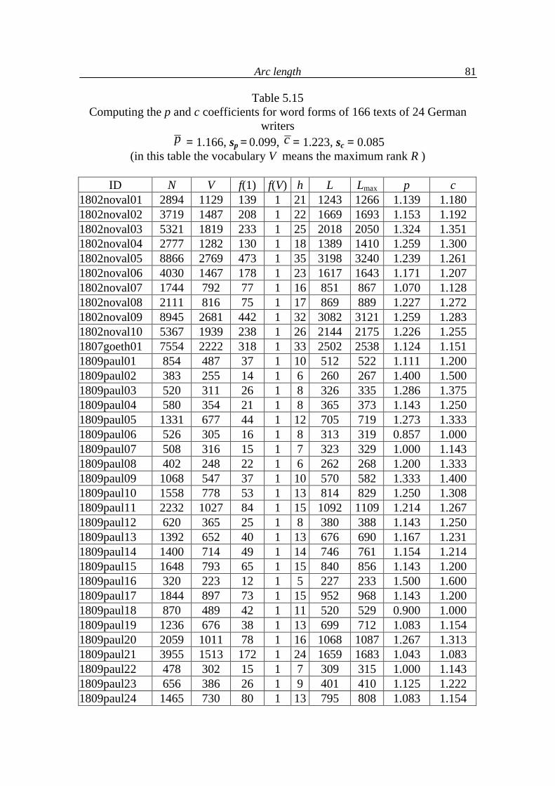
Arc length

81

Table 5.15 Computing the p and c coefficients for word forms of 166 texts of 24 German

writers p = 1.166, sp = 0.099, c = 1.223, sc = 0.085

(in this table the vocabulary V means the maximum rank R )

ID N V f(1) f(V) h L Lmax p c 1802noval01 2894 1129 139 1 21 1243 1266 1.139 1.180 1802noval02 3719 1487 208 1 22 1669 1693 1.153 1.192 1802noval03 5321 1819 233 1 25 2018 2050 1.324 1.351 1802noval04 2777 1282 130 1 18 1389 1410 1.259 1.300 1802noval05 8866 2769 473 1 35 3198 3240 1.239 1.261 1802noval06 4030 1467 178 1 23 1617 1643 1.171 1.207 1802noval07 1744 792 77 1 16 851 867 1.070 1.128 1802noval08 2111 816 75 1 17 869 889 1.227 1.272 1802noval09 8945 2681 442 1 32 3082 3121 1.259 1.283 1802noval10 5367 1939 238 1 26 2144 2175 1.226 1.255 1807goeth01 7554 2222 318 1 33 2502 2538 1.124 1.151 1809paul01 854 487 37 1 10 512 522 1.111 1.200 1809paul02 383 255 14 1 6 260 267 1.400 1.500 1809paul03 520 311 26 1 8 326 335 1.286 1.375 1809paul04 580 354 21 1 8 365 373 1.143 1.250 1809paul05 1331 677 44 1 12 705 719 1.273 1.333 1809paul06 526 305 16 1 8 313 319 0.857 1.000 1809paul07 508 316 15 1 7 323 329 1.000 1.143 1809paul08 402 248 22 1 6 262 268 1.200 1.333 1809paul09 1068 547 37 1 10 570 582 1.333 1.400 1809paul10 1558 778 53 1 13 814 829 1.250 1.308 1809paul11 2232 1027 84 1 15 1092 1109 1.214 1.267 1809paul12 620 365 25 1 8 380 388 1.143 1.250 1809paul13 1392 652 40 1 13 676 690 1.167 1.231 1809paul14 1400 714 49 1 14 746 761 1.154 1.214 1809paul15 1648 793 65 1 15 840 856 1.143 1.200 1809paul16 320 223 12 1 5 227 233 1.500 1.600 1809paul17 1844 897 73 1 15 952 968 1.143 1.200 1809paul18 870 489 42 1 11 520 529 0.900 1.000 1809paul19 1236 676 38 1 13 699 712 1.083 1.154 1809paul20 2059 1011 78 1 16 1068 1087 1.267 1.313 1809paul21 3955 1513 172 1 24 1659 1683 1.043 1.083 1809paul22 478 302 15 1 7 309 315 1.000 1.143 1809paul23 656 386 26 1 9 401 410 1.125 1.222 1809paul24 1465 730 80 1 13 795 808 1.083 1.154

Arc length

82

1809paul25 588 361 18 1 8 370 377 1.000 1.125 1809paul26 1896 887 61 1 15 930 946 1.143 1.200 1809paul27 749 410 26 1 9 426 434 1.000 1.111 1809paul28 241 172 8 1 5 174 178 1.000 1.200 1809paul29 1825 872 68 1 14 921 938 1.308 1.357 1809paul30 388 238 17 1 6 248 253 1.000 1.167 1809paul31 1630 753 72 1 14 810 823 1.000 1.071 1809paul32 163 119 6 1 4 120 123 1.000 1.250 1809paul33 596 355 23 1 8 369 376 1.000 1.125 1809paul35 1947 897 82 1 17 960 977 1.063 1.118 1809paul36 425 253 15 1 7 259 266 1.167 1.286 1809paul37 368 239 12 1 6 243 249 1.200 1.333 1809paul38 1218 636 40 1 12 660 674 1.273 1.333 1809paul39 388 248 13 1 7 253 259 1.000 1.143 1809paul40 1370 655 53 1 14 694 706 0.923 1.000 1809paul41 1032 546 43 1 11 575 587 1.200 1.273 1809paul42 1546 731 50 1 13 764 779 1.250 1.308 1809paul43 4148 1591 152 1 26 1714 1741 1.080 1.115 1809paul44 1881 896 66 1 15 943 960 1.214 1.267 1809paul45 2723 1102 155 1 18 1236 1255 1.118 1.167 1809paul46 3095 1276 99 1 21 1351 1373 1.100 1.143 1809paul47 516 319 19 1 8 330 336 0.857 1.000 1809paul48 1200 604 50 1 13 638 652 1.167 1.231 1809paul49 562 336 19 1 8 346 353 1.000 1.125 1809paul50 430 255 23 1 7 269 276 1.167 1.286 1809paul51 3222 1323 116 1 20 1413 1437 1.263 1.300 1809paul52 1731 815 71 1 15 870 884 1.000 1.067 1809paul53 1839 864 75 1 14 922 937 1.154 1.214 1809paul54 6644 2417 245 1 30 2625 2660 1.207 1.233 1809paul55 7854 2680 321 1 33 2961 2999 1.188 1.212 1809paul56 963 482 47 1 10 516 527 1.222 1.300 1813chami01 2210 884 82 1 18 944 964 1.176 1.222 1813chami02 1847 808 84 1 16 872 890 1.200 1.250 1813chami03 1428 630 70 1 14 684 698 1.077 1.143 1813chami04 3205 1209 123 1 20 1305 1330 1.316 1.350 1813chami05 2108 853 79 1 18 911 930 1.118 1.167 1813chami06 1948 801 75 1 17 853 874 1.313 1.353 1813chami07 1362 670 44 1 13 698 712 1.167 1.231 1813chami08 1870 788 80 1 16 848 866 1.200 1.250 1813chami09 1320 593 96 1 14 673 687 1.077 1.143 1813chami10 1012 536 52 1 11 575 586 1.100 1.182

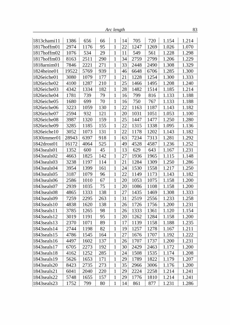
Arc length

83

1813chami11 1386 656 66 1 14 705 720 1.154 1.214 1817hoffm01 2974 1176 95 1 22 1247 1269 1.026 1.070 1817hoffm02 1076 534 29 1 11 549 561 1.228 1.298 1817hoffm03 8163 2511 290 1 34 2759 2799 1.206 1.229 1818arnim01 7846 2221 271 1 33 2448 2490 1.308 1.329 1824heine01 19522 5769 939 1 46 6648 6706 1.285 1.300 1826eiche01 3080 1079 177 1 21 1228 1254 1.300 1.333 1826eiche02 4100 1287 210 1 25 1466 1495 1.208 1.240 1826eiche03 4342 1334 182 1 28 1482 1514 1.185 1.214 1826eiche04 1781 739 79 1 16 799 816 1.133 1.188 1826eiche05 1680 699 70 1 16 750 767 1.133 1.188 1826eiche06 3223 1059 130 1 22 1163 1187 1.143 1.182 1826eiche07 2594 932 121 1 20 1031 1051 1.053 1.100 1826eiche08 3987 1320 159 1 25 1447 1477 1.250 1.280 1826eiche09 3285 1185 155 1 22 1315 1338 1.095 1.136 1826eiche10 3052 1073 131 1 22 1178 1202 1.143 1.182 1830immer01 28943 6397 918 1 63 7234 7313 1.281 1.292 1842drost01 16172 4064 525 1 49 4528 4587 1.236 1.252 1843seals01 1352 600 45 1 13 629 643 1.167 1.231 1843seals02 4663 1825 142 1 27 1936 1965 1.115 1.148 1843seals03 3238 1197 114 1 21 1284 1309 1.250 1.286 1843seals04 3954 1399 161 1 24 1530 1558 1.217 1.250 1843seals05 3187 1079 96 1 22 1149 1173 1.143 1.182 1843seals06 2586 1010 67 1 20 1053 1075 1.158 1.200 1843seals07 2939 1035 75 1 20 1086 1108 1.158 1.200 1843seals08 4865 1333 138 1 27 1435 1469 1.308 1.333 1843seals09 7259 2295 263 1 31 2519 2556 1.233 1.258 1843seals10 4838 1620 138 1 26 1726 1756 1.200 1.231 1843seals11 3785 1265 98 1 26 1333 1361 1.120 1.154 1843seals12 3019 1191 95 1 20 1262 1284 1.158 1.200 1843seals13 2370 1071 89 1 17 1139 1158 1.188 1.235 1843seals14 2744 1198 82 1 19 1257 1278 1.167 1.211 1843seals15 4786 1545 164 1 27 1676 1707 1.192 1.222 1843seals16 4497 1602 137 1 26 1707 1737 1.200 1.231 1843seals17 6705 2273 192 1 30 2429 2463 1.172 1.200 1843seals18 4162 1252 285 1 24 1508 1535 1.174 1.208 1843seals19 5626 1653 171 1 29 1789 1822 1.179 1.207 1843seals20 8423 2735 273 1 35 2966 3006 1.176 1.200 1843seals21 6041 2040 220 1 29 2224 2258 1.214 1.241 1843seals22 5748 1655 157 1 29 1776 1810 1.214 1.241 1843seals23 1752 799 80 1 14 861 877 1.231 1.286

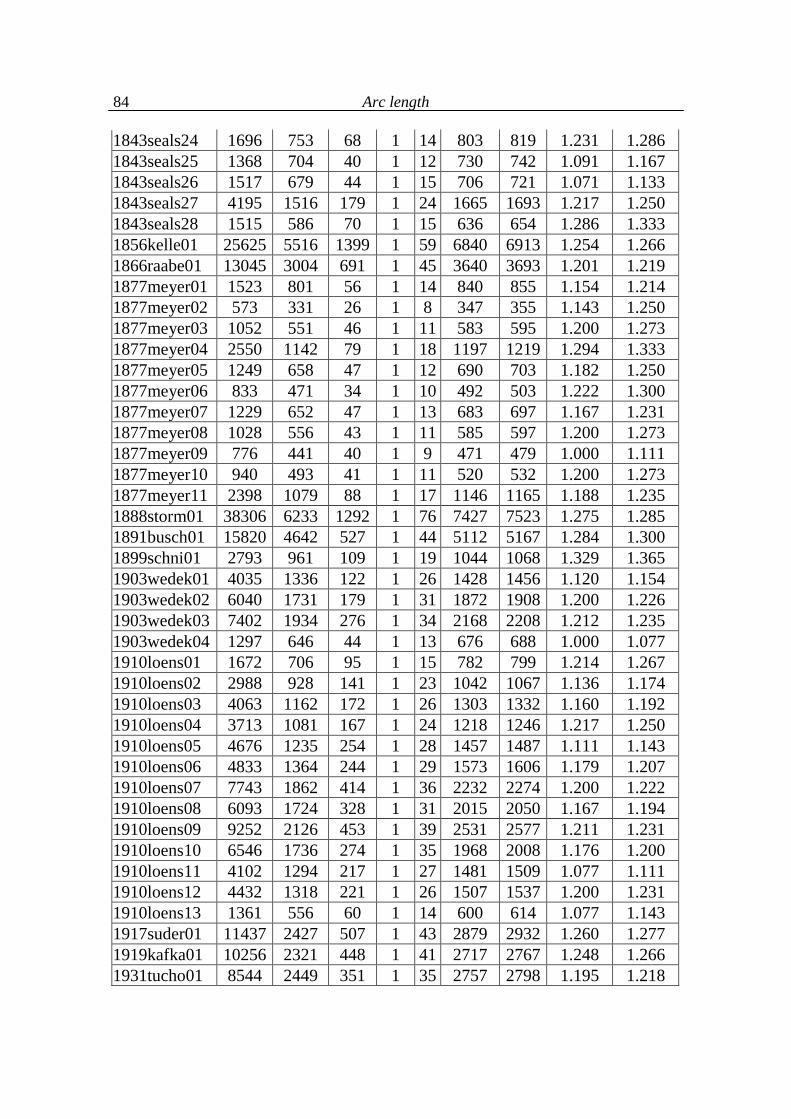
Arc length

84

1843seals24 1696 753 68 1 14 803 819 1.231 1.286 1843seals25 1368 704 40 1 12 730 742 1.091 1.167 1843seals26 1517 679 44 1 15 706 721 1.071 1.133 1843seals27 4195 1516 179 1 24 1665 1693 1.217 1.250 1843seals28 1515 586 70 1 15 636 654 1.286 1.333 1856kelle01 25625 5516 1399 1 59 6840 6913 1.254 1.266 1866raabe01 13045 3004 691 1 45 3640 3693 1.201 1.219 1877meyer01 1523 801 56 1 14 840 855 1.154 1.214 1877meyer02 573 331 26 1 8 347 355 1.143 1.250 1877meyer03 1052 551 46 1 11 583 595 1.200 1.273 1877meyer04 2550 1142 79 1 18 1197 1219 1.294 1.333 1877meyer05 1249 658 47 1 12 690 703 1.182 1.250 1877meyer06 833 471 34 1 10 492 503 1.222 1.300 1877meyer07 1229 652 47 1 13 683 697 1.167 1.231 1877meyer08 1028 556 43 1 11 585 597 1.200 1.273 1877meyer09 776 441 40 1 9 471 479 1.000 1.111 1877meyer10 940 493 41 1 11 520 532 1.200 1.273 1877meyer11 2398 1079 88 1 17 1146 1165 1.188 1.235 1888storm01 38306 6233 1292 1 76 7427 7523 1.275 1.285 1891busch01 15820 4642 527 1 44 5112 5167 1.284 1.300 1899schni01 2793 961 109 1 19 1044 1068 1.329 1.365 1903wedek01 4035 1336 122 1 26 1428 1456 1.120 1.154 1903wedek02 6040 1731 179 1 31 1872 1908 1.200 1.226 1903wedek03 7402 1934 276 1 34 2168 2208 1.212 1.235 1903wedek04 1297 646 44 1 13 676 688 1.000 1.077 1910loens01 1672 706 95 1 15 782 799 1.214 1.267 1910loens02 2988 928 141 1 23 1042 1067 1.136 1.174 1910loens03 4063 1162 172 1 26 1303 1332 1.160 1.192 1910loens04 3713 1081 167 1 24 1218 1246 1.217 1.250 1910loens05 4676 1235 254 1 28 1457 1487 1.111 1.143 1910loens06 4833 1364 244 1 29 1573 1606 1.179 1.207 1910loens07 7743 1862 414 1 36 2232 2274 1.200 1.222 1910loens08 6093 1724 328 1 31 2015 2050 1.167 1.194 1910loens09 9252 2126 453 1 39 2531 2577 1.211 1.231 1910loens10 6546 1736 274 1 35 1968 2008 1.176 1.200 1910loens11 4102 1294 217 1 27 1481 1509 1.077 1.111 1910loens12 4432 1318 221 1 26 1507 1537 1.200 1.231 1910loens13 1361 556 60 1 14 600 614 1.077 1.143 1917suder01 11437 2427 507 1 43 2879 2932 1.260 1.277 1919kafka01 10256 2321 448 1 41 2717 2767 1.248 1.266 1931tucho01 8544 2449 351 1 35 2757 2798 1.195 1.218

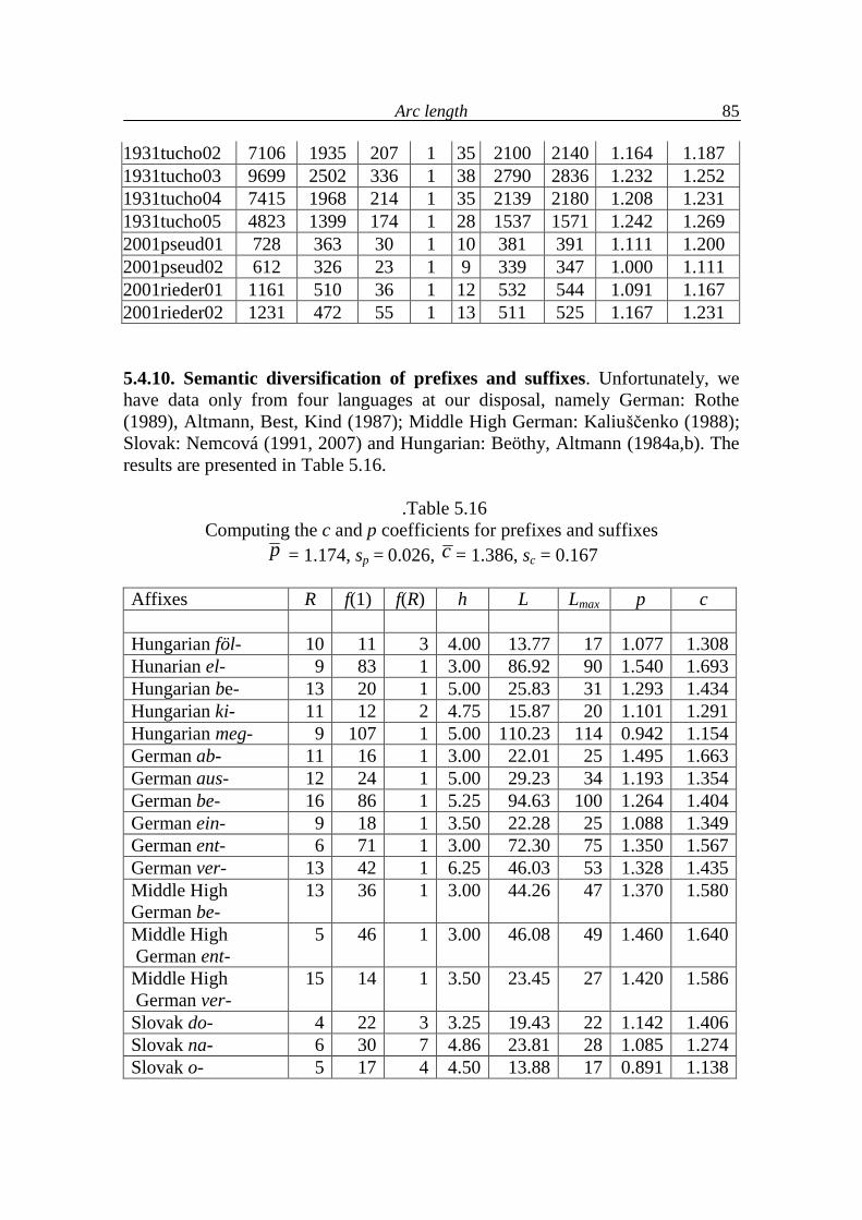
Arc length

85

1931tucho02 7106 1935 207 1 35 2100 2140 1.164 1.187 1931tucho03 9699 2502 336 1 38 2790 2836 1.232 1.252 1931tucho04 7415 1968 214 1 35 2139 2180 1.208 1.231 1931tucho05 4823 1399 174 1 28 1537 1571 1.242 1.269 2001pseud01 728 363 30 1 10 381 391 1.111 1.200 2001pseud02 612 326 23 1 9 339 347 1.000 1.111 2001rieder01 1161 510 36 1 12 532 544 1.091 1.167 2001rieder02 1231 472 55 1 13 511 525 1.167 1.231 5.4.10. Semantic diversification of prefixes and suffixes. Unfortunately, we have data only from four languages at our disposal, namely German: Rothe (1989), Altmann, Best, Kind (1987); Middle High German: Kaliu�čenko (1988); Slovak: Nemcová (1991, 2007) and Hungarian: Beöthy, Altmann (1984a,b). The results are presented in Table 5.16.

.Table 5.16

Computing the c and p coefficients for prefixes and suffixes p = 1.174, sp = 0.026, c = 1.386, sc = 0.167

Affixes R f(1) f(R) h L Lmax p c Hungarian föl- 10 11 3 4.00 13.77 17 1.077 1.308 Hunarian el- 9 83 1 3.00 86.92 90 1.540 1.693 Hungarian be- 13 20 1 5.00 25.83 31 1.293 1.434 Hungarian ki- 11 12 2 4.75 15.87 20 1.101 1.291 Hungarian meg- 9 107 1 5.00 110.23 114 0.942 1.154 German ab- 11 16 1 3.00 22.01 25 1.495 1.663 German aus- 12 24 1 5.00 29.23 34 1.193 1.354 German be- 16 86 1 5.25 94.63 100 1.264 1.404 German ein- 9 18 1 3.50 22.28 25 1.088 1.349 German ent- 6 71 1 3.00 72.30 75 1.350 1.567 German ver- 13 42 1 6.25 46.03 53 1.328 1.435 Middle High German be-

13 36 1 3.00 44.26 47 1.370 1.580

Middle High German ent-

5 46 1 3.00 46.08 49 1.460 1.640

Middle High German ver-

15 14 1 3.50 23.45 27 1.420 1.586

Slovak do- 4 22 3 3.25 19.43 22 1.142 1.406 Slovak na- 6 30 7 4.86 23.81 28 1.085 1.274 Slovak o- 5 17 4 4.50 13.88 17 0.891 1.138

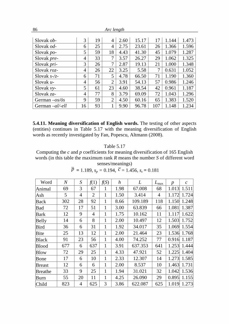
Arc length

86

Slovak ob- 3 19 4 2.60 15.17 17 1.144 1.473 Slovak od- 6 25 4 2.75 23.61 26 1.366 1.596 Slovak po- 5 59 18 4.43 41.30 45 1.079 1.287 Slovak pre- 4 33 7 3.57 26.27 29 1.062 1.325 Slovak pri- 3 26 7 2.87 19.13 21 1.000 1.348 Slovak roz- 4 26 22 3.25 5.58 7 0.631 1.052 Slovak s-/z- 6 71 5 4.78 66.50 71 1.190 1.360 Slovak u- 4 56 2 3.91 54.13 57 0.986 1.246 Slovak vy- 5 61 23 4.60 38.54 42 0.961 1.187 Slovak za- 4 77 8 3.79 69.09 72 1.043 1.296 German –os/ös 9 59 2 4.50 60.16 65 1.383 1.520 German –al/-ell 16 93 1 9.90 96.78 107 1.148 1.234

5.4.11. Meaning diversification of English words. The testing of other aspects (entities) continues in Table 5.17 with the meaning diversification of English words as recently investigated by Fan, Popescu, Altmann (2008).

Table 5.17

Computing the c and p coefficients for meaning diversification of 165 English words (in this table the maximum rank R means the number S of different word

senses/meanings) p = 1.189, sp = 0.194, c = 1.456, sc = 0.181

Word N S f(1) f(S) h L Lmax p c

Animal 69 3 67 1 1.98 67.008 68 1.013 1.511 Ash 5 4 2 1 1.50 3.414 4 1.172 1.724 Back 302 28 92 1 8.66 109.189 118 1.150 1.248 Bad 72 17 51 1 3.00 63.839 66 1.081 1.387 Bark 12 9 4 1 1.75 10.162 11 1.117 1.622 Belly 14 6 8 1 2.00 10.497 12 1.503 1.752 Bird 36 6 31 1 1.92 34.017 35 1.069 1.554 Bite 25 13 12 1 2.00 21.464 23 1.536 1.768 Black 91 23 56 1 4.00 74.252 77 0.916 1.187 Blood 677 6 637 1 3.91 637.353 641 1.253 1.444 Blow 72 29 25 1 4.33 47.921 52 1.225 1.404 Bone 17 6 10 1 2.33 12.307 14 1.273 1.585 Breast 12 6 6 1 2.00 8.537 10 1.463 1.731 Breathe 33 9 25 1 1.94 31.021 32 1.042 1.536 Burn 55 20 11 1 4.25 26.090 29 0.895 1.155 Child 823 4 625 3 3.86 622.087 625 1.019 1.273

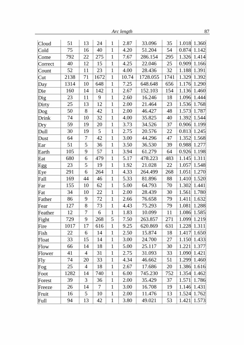
Arc length

87

Cloud 51 13 24 1 2.87 33.096 35 1.018 1.360 Cold 75 16 40 1 4.20 51.204 54 0.874 1.142 Come 792 22 275 1 7.67 286.154 295 1.326 1.414 Correct 40 12 15 1 4.25 22.046 25 0.909 1.166 Count 52 11 23 1 4.00 28.436 32 1.188 1.391 Cut 2138 71 1672 1 10.74 1728.055 1741 1.329 1.392 Day 1314 10 648 1 7.25 648.648 656 1.176 1.290 Die 160 14 142 1 2.67 152.103 154 1.136 1.460 Dig 23 11 9 1 2.60 16.246 18 1.096 1.444 Dirty 25 13 12 1 2.00 21.464 23 1.536 1.768 Dog 50 8 42 1 2.00 46.427 48 1.573 1.787 Drink 74 10 32 1 4.00 35.825 40 1.392 1.544 Dry 59 19 20 1 3.73 34.526 37 0.906 1.199 Dull 30 19 5 1 2.75 20.576 22 0.813 1.245 Dust 64 7 42 1 3.00 44.296 47 1.352 1.568 Ear 51 5 36 1 3.50 36.530 39 0.988 1.277 Earth 105 9 57 1 3.94 61.279 64 0.926 1.198 Eat 680 6 479 1 5.17 478.223 483 1.145 1.311 Egg 23 5 19 1 1.92 21.028 22 1.057 1.548 Eye 291 6 264 1 4.33 264.499 268 1.051 1.270 Fall 169 44 46 1 5.33 81.896 88 1.410 1.520 Far 155 10 62 1 5.00 64.793 70 1.302 1.441 Fat 34 10 22 1 2.00 28.439 30 1.561 1.780 Father 86 9 72 1 2.66 76.658 79 1.411 1.632 Fear 127 8 73 1 4.43 75.293 79 1.081 1.288 Feather 12 7 6 1 1.83 10.099 11 1.086 1.585 Fight 729 9 268 5 7.50 263.857 271 1.099 1.219 Fire 1017 17 616 1 9.25 620.869 631 1.228 1.311 Fish 22 6 14 1 2.50 15.874 18 1.417 1.650 Float 33 15 14 1 3.00 24.700 27 1.150 1.433 Flow 66 14 18 1 5.00 25.117 30 1.221 1.377 Flower 41 4 31 1 2.75 31.093 33 1.090 1.421 Fly 74 20 33 1 4.34 46.662 51 1.299 1.460 Fog 25 4 18 1 2.67 17.686 20 1.386 1.616 Foot 1282 14 740 1 6.00 745.230 752 1.354 1.462 Forest 39 3 36 1 2.00 35.429 37 1.571 1.786 Freeze 26 14 7 1 3.00 16.708 19 1.146 1.431 Fruit 16 5 10 1 2.00 11.476 13 1.524 1.762 Full 94 13 42 1 3.80 49.021 53 1.421 1.573

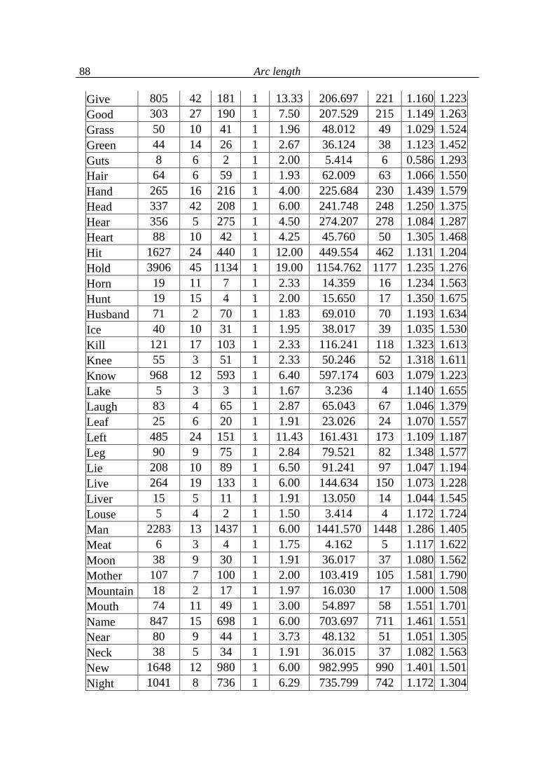
Arc length

88

Give 805 42 181 1 13.33 206.697 221 1.160 1.223 Good 303 27 190 1 7.50 207.529 215 1.149 1.263 Grass 50 10 41 1 1.96 48.012 49 1.029 1.524 Green 44 14 26 1 2.67 36.124 38 1.123 1.452 Guts 8 6 2 1 2.00 5.414 6 0.586 1.293 Hair 64 6 59 1 1.93 62.009 63 1.066 1.550 Hand 265 16 216 1 4.00 225.684 230 1.439 1.579 Head 337 42 208 1 6.00 241.748 248 1.250 1.375 Hear 356 5 275 1 4.50 274.207 278 1.084 1.287 Heart 88 10 42 1 4.25 45.760 50 1.305 1.468 Hit 1627 24 440 1 12.00 449.554 462 1.131 1.204 Hold 3906 45 1134 1 19.00 1154.762 1177 1.235 1.276 Horn 19 11 7 1 2.33 14.359 16 1.234 1.563 Hunt 19 15 4 1 2.00 15.650 17 1.350 1.675 Husband 71 2 70 1 1.83 69.010 70 1.193 1.634 Ice 40 10 31 1 1.95 38.017 39 1.035 1.530 Kill 121 17 103 1 2.33 116.241 118 1.323 1.613 Knee 55 3 51 1 2.33 50.246 52 1.318 1.611 Know 968 12 593 1 6.40 597.174 603 1.079 1.223 Lake 5 3 3 1 1.67 3.236 4 1.140 1.655 Laugh 83 4 65 1 2.87 65.043 67 1.046 1.379 Leaf 25 6 20 1 1.91 23.026 24 1.070 1.557 Left 485 24 151 1 11.43 161.431 173 1.109 1.187 Leg 90 9 75 1 2.84 79.521 82 1.348 1.577 Lie 208 10 89 1 6.50 91.241 97 1.047 1.194 Live 264 19 133 1 6.00 144.634 150 1.073 1.228 Liver 15 5 11 1 1.91 13.050 14 1.044 1.545 Louse 5 4 2 1 1.50 3.414 4 1.172 1.724 Man 2283 13 1437 1 6.00 1441.570 1448 1.286 1.405 Meat 6 3 4 1 1.75 4.162 5 1.117 1.622 Moon 38 9 30 1 1.91 36.017 37 1.080 1.562 Mother 107 7 100 1 2.00 103.419 105 1.581 1.790 Mountain 18 2 17 1 1.97 16.030 17 1.000 1.508 Mouth 74 11 49 1 3.00 54.897 58 1.551 1.701 Name 847 15 698 1 6.00 703.697 711 1.461 1.551 Near 80 9 44 1 3.73 48.132 51 1.051 1.305 Neck 38 5 34 1 1.91 36.015 37 1.082 1.563 New 1648 12 980 1 6.00 982.995 990 1.401 1.501 Night 1041 8 736 1 6.29 735.799 742 1.172 1.304

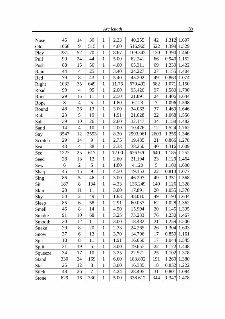
Arc length

89

Nose 45 14 30 1 2.33 40.255 42 1.312 1.607 Old 1066 9 515 1 4.60 516.965 522 1.399 1.529 Play 331 52 70 1 8.67 109.342 120 1.390 1.460 Pull 90 24 44 1 5.00 62.241 66 0.940 1.152 Push 88 15 56 1 4.00 65.311 69 1.230 1.422 Rain 44 4 25 1 3.40 24.227 27 1.155 1.404 Red 79 8 43 1 5.40 45.202 49 0.863 1.074 Right 1032 35 649 1 11.75 670.492 682 1.071 1.150 Road 99 4 95 1 2.00 95.420 97 1.580 1.790 Root 29 15 11 1 2.50 21.891 24 1.406 1.644 Rope 8 4 5 1 1.80 6.123 7 1.096 1.598 Round 48 26 13 1 3.00 34.062 37 1.469 1.646 Rub 23 5 19 1 1.91 21.028 22 1.068 1.556 Salt 39 10 26 1 2.60 32.147 34 1.158 1.482 Sand 14 4 10 1 2.00 10.476 12 1.524 1.762 Say 3547 12 2593 1 8.20 2593.961 2603 1.255 1.346 Scratch 29 14 9 1 2.75 19.485 21 0.866 1.278 Sea 43 4 38 1 2.33 38.250 40 1.316 1.609 See 1227 25 617 1 12.00 626.970 640 1.185 1.252 Seed 28 13 12 1 2.60 21.194 23 1.129 1.464 Sew 6 2 5 1 1.80 4.120 5 1.100 1.600 Sharp 45 15 9 1 4.50 19.153 22 0.813 1.077 Sing 86 5 46 1 3.00 46.297 49 1.351 1.568 Sit 187 8 134 1 4.33 136.249 140 1.126 1.328 Skin 28 11 11 1 3.00 17.891 20 1.055 1.370 Sky 50 2 49 1 1.83 48.010 49 1.193 1.634 Sleep 85 6 58 1 2.91 60.037 62 1.028 1.362 Smell 46 8 14 1 4.50 15.994 20 1.145 1.335 Smoke 91 10 68 1 3.25 73.233 76 1.230 1.467 Smooth 30 12 11 1 3.00 18.482 21 1.259 1.506 Snake 29 8 20 1 2.33 24.265 26 1.304 1.603 Snow 37 6 13 1 3.70 14.706 17 0.850 1.161 Spit 18 8 11 1 1.91 16.050 17 1.044 1.545 Split 31 19 5 1 3.00 19.657 22 1.172 1.448 Squeeze 34 17 10 1 3.25 22.521 25 1.102 1.378 Stand 330 24 169 1 6.60 183.892 191 1.269 1.380 Star 25 12 8 1 3.00 16.335 18 0.832 1.222 Stick 48 26 7 1 4.24 28.405 31 0.801 1.084 Stone 629 16 330 1 5.00 338.612 344 1.347 1.478

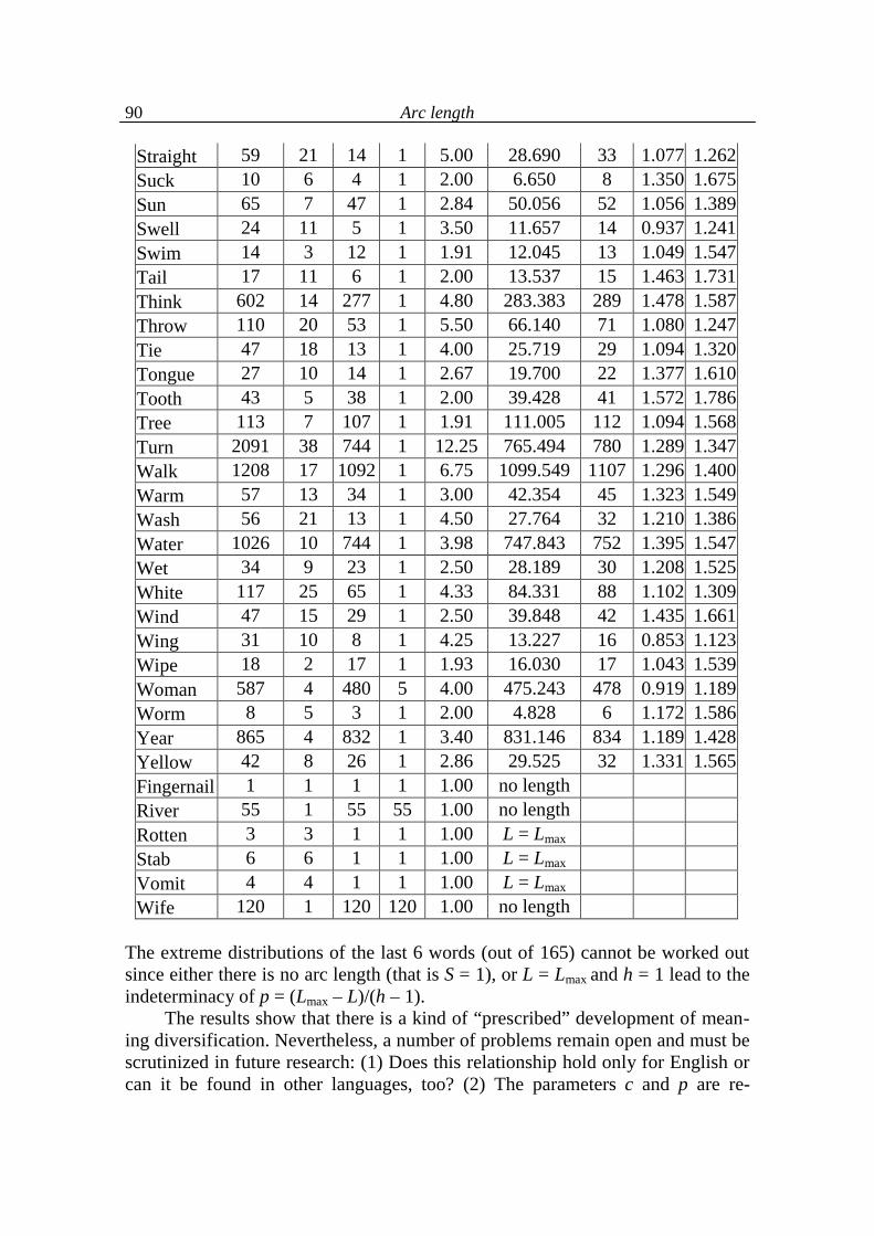
Arc length

90

Straight 59 21 14 1 5.00 28.690 33 1.077 1.262 Suck 10 6 4 1 2.00 6.650 8 1.350 1.675 Sun 65 7 47 1 2.84 50.056 52 1.056 1.389 Swell 24 11 5 1 3.50 11.657 14 0.937 1.241 Swim 14 3 12 1 1.91 12.045 13 1.049 1.547 Tail 17 11 6 1 2.00 13.537 15 1.463 1.731 Think 602 14 277 1 4.80 283.383 289 1.478 1.587 Throw 110 20 53 1 5.50 66.140 71 1.080 1.247 Tie 47 18 13 1 4.00 25.719 29 1.094 1.320 Tongue 27 10 14 1 2.67 19.700 22 1.377 1.610 Tooth 43 5 38 1 2.00 39.428 41 1.572 1.786 Tree 113 7 107 1 1.91 111.005 112 1.094 1.568 Turn 2091 38 744 1 12.25 765.494 780 1.289 1.347 Walk 1208 17 1092 1 6.75 1099.549 1107 1.296 1.400 Warm 57 13 34 1 3.00 42.354 45 1.323 1.549 Wash 56 21 13 1 4.50 27.764 32 1.210 1.386 Water 1026 10 744 1 3.98 747.843 752 1.395 1.547 Wet 34 9 23 1 2.50 28.189 30 1.208 1.525 White 117 25 65 1 4.33 84.331 88 1.102 1.309 Wind 47 15 29 1 2.50 39.848 42 1.435 1.661 Wing 31 10 8 1 4.25 13.227 16 0.853 1.123 Wipe 18 2 17 1 1.93 16.030 17 1.043 1.539 Woman 587 4 480 5 4.00 475.243 478 0.919 1.189 Worm 8 5 3 1 2.00 4.828 6 1.172 1.586 Year 865 4 832 1 3.40 831.146 834 1.189 1.428 Yellow 42 8 26 1 2.86 29.525 32 1.331 1.565 Fingernail 1 1 1 1 1.00 no length River 55 1 55 55 1.00 no length Rotten 3 3 1 1 1.00 L = Lmax Stab 6 6 1 1 1.00 L = Lmax Vomit 4 4 1 1 1.00 L = Lmax Wife 120 1 120 120 1.00 no length

The extreme distributions of the last 6 words (out of 165) cannot be worked out since either there is no arc length (that is S = 1), or L = Lmax and h = 1 lead to the indeterminacy of p = (Lmax – L)/(h – 1).

The results show that there is a kind of “prescribed” development of mean-ing diversification. Nevertheless, a number of problems remain open and must be scrutinized in future research: (1) Does this relationship hold only for English or can it be found in other languages, too? (2) The parameters c and p are re-

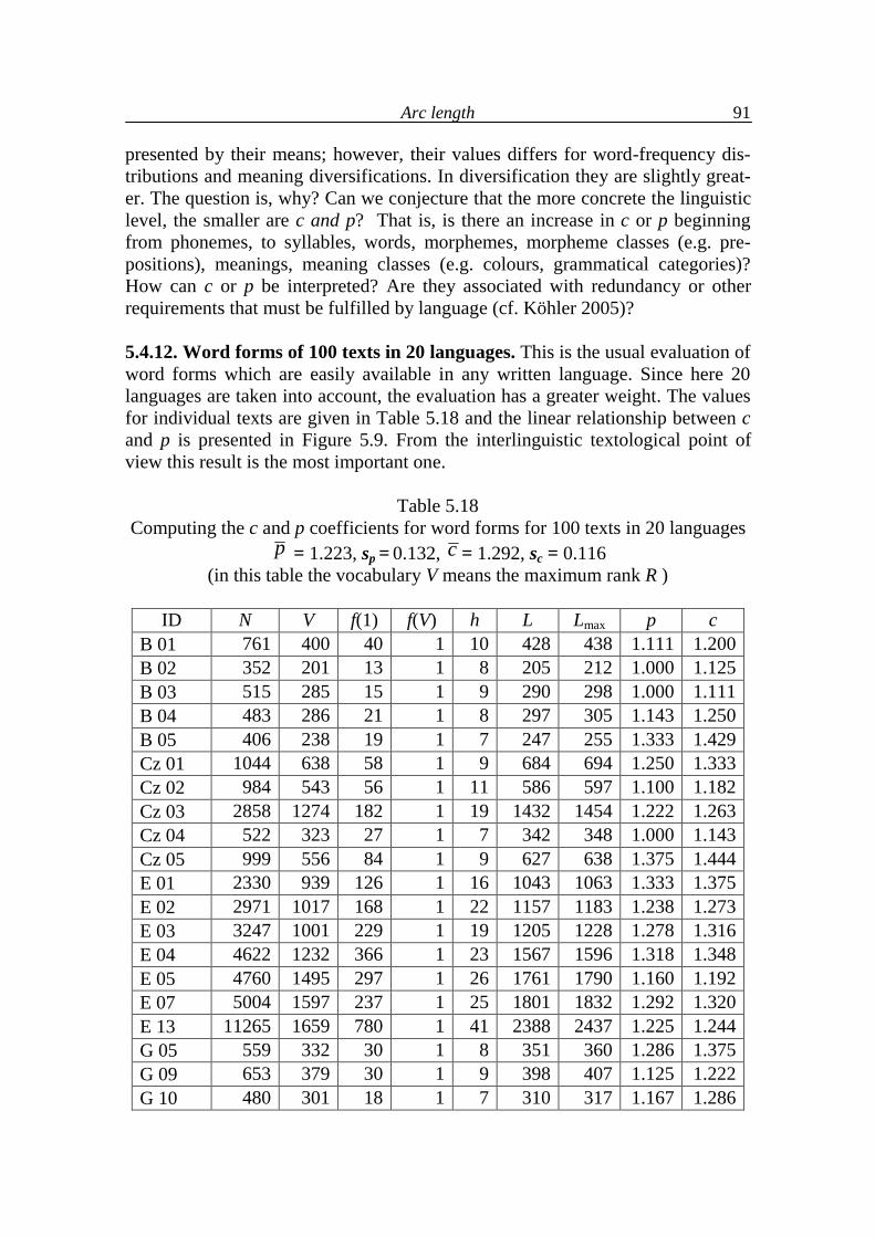
Arc length

91

presented by their means; however, their values differs for word-frequency dis-tributions and meaning diversifications. In diversification they are slightly great-er. The question is, why? Can we conjecture that the more concrete the linguistic level, the smaller are c and p? That is, is there an increase in c or p beginning from phonemes, to syllables, words, morphemes, morpheme classes (e.g. pre-positions), meanings, meaning classes (e.g. colours, grammatical categories)? How can c or p be interpreted? Are they associated with redundancy or other requirements that must be fulfilled by language (cf. Köhler 2005)? 5.4.12. Word forms of 100 texts in 20 languages. This is the usual evaluation of word forms which are easily available in any written language. Since here 20 languages are taken into account, the evaluation has a greater weight. The values for individual texts are given in Table 5.18 and the linear relationship between c and p is presented in Figure 5.9. From the interlinguistic textological point of view this result is the most important one.

Table 5.18 Computing the c and p coefficients for word forms for 100 texts in 20 languages

p = 1.223, sp = 0.132, c = 1.292, sc = 0.116 (in this table the vocabulary V means the maximum rank R )

ID N V f(1) f(V) h L Lmax p c

B 01 761 400 40 1 10 428 438 1.111 1.200 B 02 352 201 13 1 8 205 212 1.000 1.125 B 03 515 285 15 1 9 290 298 1.000 1.111 B 04 483 286 21 1 8 297 305 1.143 1.250 B 05 406 238 19 1 7 247 255 1.333 1.429 Cz 01 1044 638 58 1 9 684 694 1.250 1.333 Cz 02 984 543 56 1 11 586 597 1.100 1.182 Cz 03 2858 1274 182 1 19 1432 1454 1.222 1.263 Cz 04 522 323 27 1 7 342 348 1.000 1.143 Cz 05 999 556 84 1 9 627 638 1.375 1.444 E 01 2330 939 126 1 16 1043 1063 1.333 1.375 E 02 2971 1017 168 1 22 1157 1183 1.238 1.273 E 03 3247 1001 229 1 19 1205 1228 1.278 1.316 E 04 4622 1232 366 1 23 1567 1596 1.318 1.348 E 05 4760 1495 297 1 26 1761 1790 1.160 1.192 E 07 5004 1597 237 1 25 1801 1832 1.292 1.320 E 13 11265 1659 780 1 41 2388 2437 1.225 1.244 G 05 559 332 30 1 8 351 360 1.286 1.375 G 09 653 379 30 1 9 398 407 1.125 1.222 G 10 480 301 18 1 7 310 317 1.167 1.286

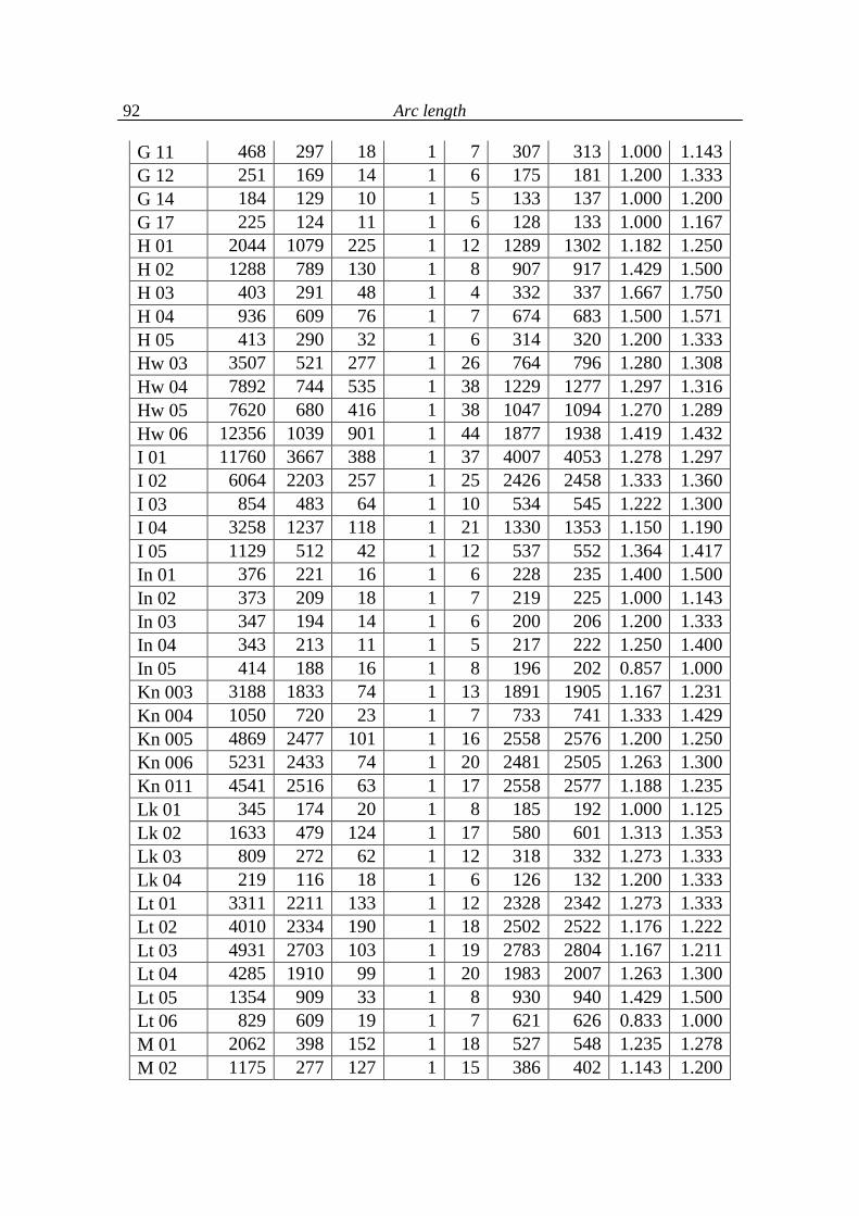
Arc length

92

G 11 468 297 18 1 7 307 313 1.000 1.143 G 12 251 169 14 1 6 175 181 1.200 1.333 G 14 184 129 10 1 5 133 137 1.000 1.200 G 17 225 124 11 1 6 128 133 1.000 1.167 H 01 2044 1079 225 1 12 1289 1302 1.182 1.250 H 02 1288 789 130 1 8 907 917 1.429 1.500 H 03 403 291 48 1 4 332 337 1.667 1.750 H 04 936 609 76 1 7 674 683 1.500 1.571 H 05 413 290 32 1 6 314 320 1.200 1.333 Hw 03 3507 521 277 1 26 764 796 1.280 1.308 Hw 04 7892 744 535 1 38 1229 1277 1.297 1.316 Hw 05 7620 680 416 1 38 1047 1094 1.270 1.289 Hw 06 12356 1039 901 1 44 1877 1938 1.419 1.432 I 01 11760 3667 388 1 37 4007 4053 1.278 1.297 I 02 6064 2203 257 1 25 2426 2458 1.333 1.360 I 03 854 483 64 1 10 534 545 1.222 1.300 I 04 3258 1237 118 1 21 1330 1353 1.150 1.190 I 05 1129 512 42 1 12 537 552 1.364 1.417 In 01 376 221 16 1 6 228 235 1.400 1.500 In 02 373 209 18 1 7 219 225 1.000 1.143 In 03 347 194 14 1 6 200 206 1.200 1.333 In 04 343 213 11 1 5 217 222 1.250 1.400 In 05 414 188 16 1 8 196 202 0.857 1.000 Kn 003 3188 1833 74 1 13 1891 1905 1.167 1.231 Kn 004 1050 720 23 1 7 733 741 1.333 1.429 Kn 005 4869 2477 101 1 16 2558 2576 1.200 1.250 Kn 006 5231 2433 74 1 20 2481 2505 1.263 1.300 Kn 011 4541 2516 63 1 17 2558 2577 1.188 1.235 Lk 01 345 174 20 1 8 185 192 1.000 1.125 Lk 02 1633 479 124 1 17 580 601 1.313 1.353 Lk 03 809 272 62 1 12 318 332 1.273 1.333 Lk 04 219 116 18 1 6 126 132 1.200 1.333 Lt 01 3311 2211 133 1 12 2328 2342 1.273 1.333 Lt 02 4010 2334 190 1 18 2502 2522 1.176 1.222 Lt 03 4931 2703 103 1 19 2783 2804 1.167 1.211 Lt 04 4285 1910 99 1 20 1983 2007 1.263 1.300 Lt 05 1354 909 33 1 8 930 940 1.429 1.500 Lt 06 829 609 19 1 7 621 626 0.833 1.000 M 01 2062 398 152 1 18 527 548 1.235 1.278 M 02 1175 277 127 1 15 386 402 1.143 1.200

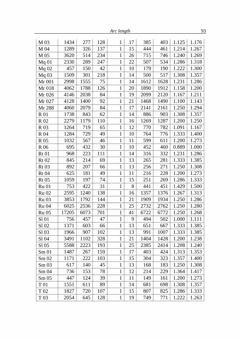
Arc length

93

M 03 1434 277 128 1 17 385 403 1.125 1.176 M 04 1289 326 137 1 15 444 461 1.214 1.267 M 05 3620 514 234 1 26 715 746 1.240 1.269 Mq 01 2330 289 247 1 22 507 534 1.286 1.318 Mq 02 457 150 42 1 10 179 190 1.222 1.300 Mq 03 1509 301 218 1 14 500 517 1.308 1.357 Mr 001 2998 1555 75 1 14 1612 1628 1.231 1.286 Mr 018 4062 1788 126 1 20 1890 1912 1.158 1.200 Mr 026 4146 2038 84 1 19 2099 2120 1.167 1.211 Mr 027 4128 1400 92 1 21 1468 1490 1.100 1.143 Mr 288 4060 2079 84 1 17 2141 2161 1.250 1.294 R 01 1738 843 62 1 14 886 903 1.308 1.357 R 02 2279 1179 110 1 16 1269 1287 1.200 1.250 R 03 1264 719 65 1 12 770 782 1.091 1.167 R 04 1284 729 49 1 10 764 776 1.333 1.400 R 05 1032 567 46 1 11 599 611 1.200 1.273 R 06 695 432 30 1 10 452 460 0.889 1.000 Rt 01 968 223 111 1 14 316 332 1.231 1.286 Rt 02 845 214 69 1 13 265 281 1.333 1.385 Rt 03 892 207 66 1 13 256 271 1.250 1.308 Rt 04 625 181 49 1 11 216 228 1.200 1.273 Rt 05 1059 197 74 1 15 251 269 1.286 1.333 Ru 01 753 422 31 1 8 441 451 1.429 1.500 Ru 02 2595 1240 138 1 16 1357 1376 1.267 1.313 Ru 03 3853 1792 144 1 21 1909 1934 1.250 1.286 Ru 04 6025 2536 228 1 25 2732 2762 1.250 1.280 Ru 05 17205 6073 701 1 41 6722 6772 1.250 1.268 Sl 01 756 457 47 1 9 494 502 1.000 1.111 Sl 02 1371 603 66 1 13 651 667 1.333 1.385 Sl 03 1966 907 102 1 13 991 1007 1.333 1.385 Sl 04 3491 1102 328 1 21 1404 1428 1.200 1.238 Sl 05 5588 2223 193 1 25 2385 2414 1.208 1.240 Sm 01 1487 267 159 1 17 403 424 1.313 1.353 Sm 02 1171 222 103 1 15 304 323 1.357 1.400 Sm 03 617 140 45 1 13 168 183 1.250 1.308 Sm 04 736 153 78 1 12 214 229 1.364 1.417 Sm 05 447 124 39 1 11 149 161 1.200 1.273 T 01 1551 611 89 1 14 681 698 1.308 1.357 T 02 1827 720 107 1 15 807 825 1.286 1.333 T 03 2054 645 128 1 19 749 771 1.222 1.263

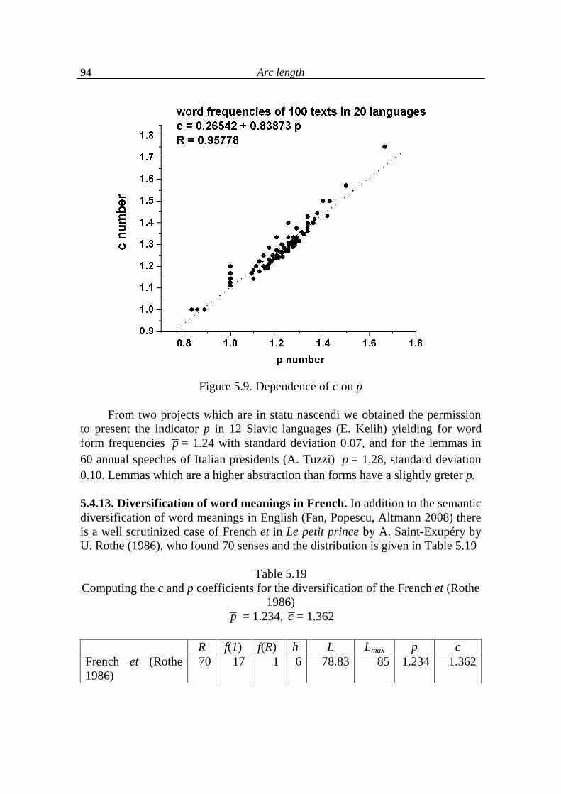
Arc length

94

Figure 5.9. Dependence of c on p

From two projects which are in statu nascendi we obtained the permission to present the indicator p in 12 Slavic languages (E. Kelih) yielding for word form frequencies p = 1.24 with standard deviation 0.07, and for the lemmas in 60 annual speeches of Italian presidents (A. Tuzzi) p = 1.28, standard deviation 0.10. Lemmas which are a higher abstraction than forms have a slightly greter p. 5.4.13. Diversification of word meanings in French. In addition to the semantic diversification of word meanings in English (Fan, Popescu, Altmann 2008) there is a well scrutinized case of French et in Le petit prince by A. Saint-Exupéry by U. Rothe (1986), who found 70 senses and the distribution is given in Table 5.19

Table 5.19 Computing the c and p coefficients for the diversification of the French et (Rothe

1986) p = 1.234, c = 1.362

R f(1) f(R) h L Lmax p c

French et (Rothe 1986)

70 17 1 6 78.83 85 1.234 1.362

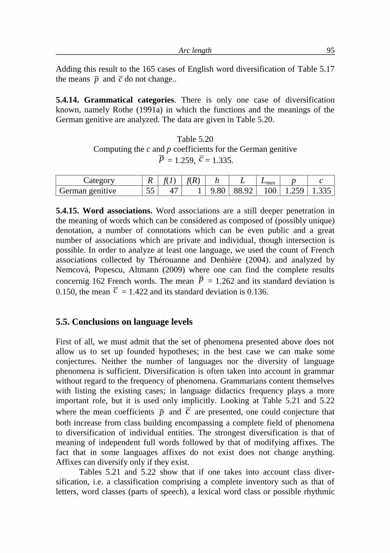
Arc length

95

Adding this result to the 165 cases of English word diversification of Table 5.17 the means p and c do not change.. 5.4.14. Grammatical categories. There is only one case of diversification known, namely Rothe (1991a) in which the functions and the meanings of the German genitive are analyzed. The data are given in Table 5.20.

Table 5.20 Computing the c and p coefficients for the German genitive

p = 1.259, c = 1.335.

Category R f(1) f(R) h L Lmax p c German genitive 55 47 1 9.80 88.92 100 1.259 1.335

5.4.15. Word associations. Word associations are a still deeper penetration in the meaning of words which can be considered as composed of (possibly unique) denotation, a number of connotations which can be even public and a great number of associations which are private and individual, though intersection is possible. In order to analyze at least one language, we used the count of French associations collected by Thérouanne and Denhière (2004). and analyzed by Nemcová, Popescu, Altmann (2009) where one can find the complete results concernig 162 French words. The mean p = 1.262 and its standard deviation is 0.150, the mean c = 1.422 and its standard deviation is 0.136. 5.5. Conclusions on language levels First of all, we must admit that the set of phenomena presented above does not allow us to set up founded hypotheses; in the best case we can make some conjectures. Neither the number of languages nor the diversity of language phenomena is sufficient. Diversification is often taken into account in grammar without regard to the frequency of phenomena. Grammarians content themselves with listing the existing cases; in language didactics frequency plays a more important role, but it is used only implicitly. Looking at Table 5.21 and 5.22 where the mean coefficients p and c are presented, one could conjecture that both increase from class building encompassing a complete field of phenomena to diversification of individual entities. The strongest diversification is that of meaning of independent full words followed by that of modifying affixes. The fact that in some languages affixes do not exist does not change anything. Affixes can diversify only if they exist.

Tables 5.21 and 5.22 show that if one takes into account class diver-sification, i.e. a classification comprising a complete inventory such as that of letters, word classes (parts of speech), a lexical word class or possible rhythmic

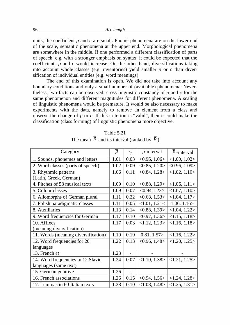
Arc length

96

units, the coefficient p and c are small. Phonic phenomena are on the lower end of the scale, semantic phenomena at the upper end. Morphological phenomena are somewhere in the middle. If one performed a different classification of parts of speech, e.g. with a stronger emphasis on syntax, it could be expected that the coefficients p and c would increase. On the other hand, diversifications taking into account whole classes (e.g. inventories) yield smaller p or c than diver-sification of individual entities (e.g. word meanings). The end of this examination is open. We did not take into account any boundary conditions and only a small number of (available) phenomena. Never-theless, two facts can be observed: cross-linguistic constancy of p and c for the same phenomenon and different magnitudes for different phenomena. A scaling of linguistic phenomena would be premature. It would be also necessary to make experiments with the data, namely to remove an element from a class and observe the change of p or c. If this criterion is “valid”, then it could make the classification (class forming) of linguistic phenomena more objective.

Table 5.21

The mean p and its interval (ranked by p )

Category p sp p-interval p -interval 1. Sounds, phonemes and letters 1.01 0.03 <0.96, 1.06> <1.00, 1.02> 2. Word classes (parts of speech) 1.02 0.09 <0.85, 1.20> <0.96, 1.09> 3. Rhythmic patterns (Latin, Greek, German)

1.06 0.11 <0.84, 1.28> <1.02, 1.10>

4. Pitches of 58 musical texts 1.09 0.10 <0.88, 1.29> <1.06, 1.11> 5. Colour classes 1.09 0.07 <0.94,1.23> <1.07, 1.10> 6. Allomorphs of German plural 1.11 0.22 <0.68, 1.53> <1.04, 1.17> 7. Polish paradigmatic classes 1.11 0.05 <1.01, 1.21< 1.06, 1.16> 8. Auxiliaries 1.13 0.14 <0.88, 1.39> <1.04, 1.22> 9. Word frequencies for German 1.17 0.10 <0.97, 1.36> <1.15, 1.18> 10. Affixes (meaning diversification)

1.17 0.03 <1.12, 1.23> <1.16, 1.18>

11. Words (meaning diversification) 1.19 0.19 0.81, 1.57> <1.16, 1.22> 12. Word frequencies for 20 languages

1.22 0.13 <0.96, 1.48> <1.20, 1.25>

13. French et 1.23 - - - 14. Word frequencies in 12 Slavic languages (same text)

1.24 0.07 <1.10, 1.38> <1.21, 1.25>

15. German genitive 1.26 - - - 16. French associations 1.26 0.15 <0.94, 1.56> <1.24, 1.28> 17. Lemmas in 60 Italian texts 1.28 0.10 <1.08, 1.48> <1.25, 1.31>

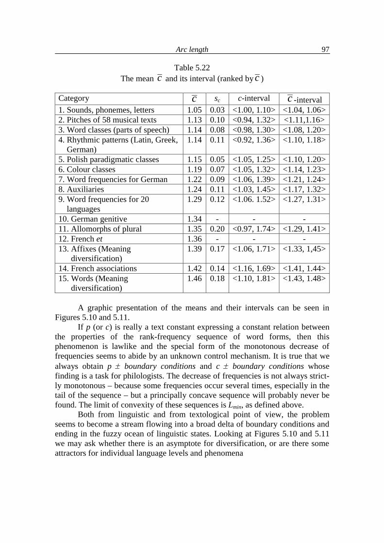
Arc length

97

Table 5.22 The mean c and its interval (ranked by c )

Category c sc c-interval c -interval 1. Sounds, phonemes, letters 1.05 0.03 <1.00, 1.10> <1.04, 1.06> 2. Pitches of 58 musical texts 1.13 0.10 <0.94, 1.32> <1.11,1.16> 3. Word classes (parts of speech) 1.14 0.08 <0.98, 1.30> <1.08, 1.20> 4. Rhythmic patterns (Latin, Greek, German)

1.14 0.11 <0.92, 1.36> <1.10, 1.18>

5. Polish paradigmatic classes 1.15 0.05 <1.05, 1.25> <1.10, 1.20> 6. Colour classes 1.19 0.07 <1.05, 1.32> <1.14, 1.23> 7. Word frequencies for German 1.22 0.09 <1.06, 1.39> <1.21, 1.24> 8. Auxiliaries 1.24 0.11 <1.03, 1.45> <1.17, 1.32> 9. Word frequencies for 20 languages

1.29 0.12 <1.06. 1.52> <1.27, 1.31>

10. German genitive 1.34 - - - 11. Allomorphs of plural 1.35 0.20 <0.97, 1.74> <1.29, 1.41> 12. French et 1.36 - - - 13. Affixes (Meaning diversification)

1.39 0.17 <1.06, 1.71> <1.33, 1,45>

14. French associations 1.42 0.14 <1.16, 1.69> <1.41, 1.44> 15. Words (Meaning diversification)

1.46 0.18 <1.10, 1.81> <1.43, 1.48>

A graphic presentation of the means and their intervals can be seen in Figures 5.10 and 5.11. If p (or c) is really a text constant expressing a constant relation between the properties of the rank-frequency sequence of word forms, then this phenomenon is lawlike and the special form of the monotonous decrease of frequencies seems to abide by an unknown control mechanism. It is true that we always obtain p boundary conditions and c boundary conditions whose finding is a task for philologists. The decrease of frequencies is not always strict-ly monotonous – because some frequencies occur several times, especially in the tail of the sequence – but a principally concave sequence will probably never be found. The limit of convexity of these sequences is Lmin, as defined above. Both from linguistic and from textological point of view, the problem seems to become a stream flowing into a broad delta of boundary conditions and ending in the fuzzy ocean of linguistic states. Looking at Figures 5.10 and 5.11 we may ask whether there is an asymptote for diversification, or are there some attractors for individual language levels and phenomena

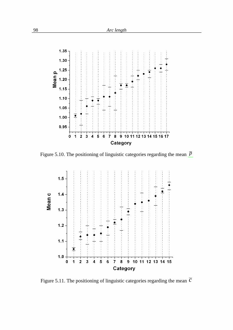
Arc length

98

Figure 5.10. The positioning of linguistic categories regarding the mean p

Figure 5.11. The positioning of linguistic categories regarding the mean c

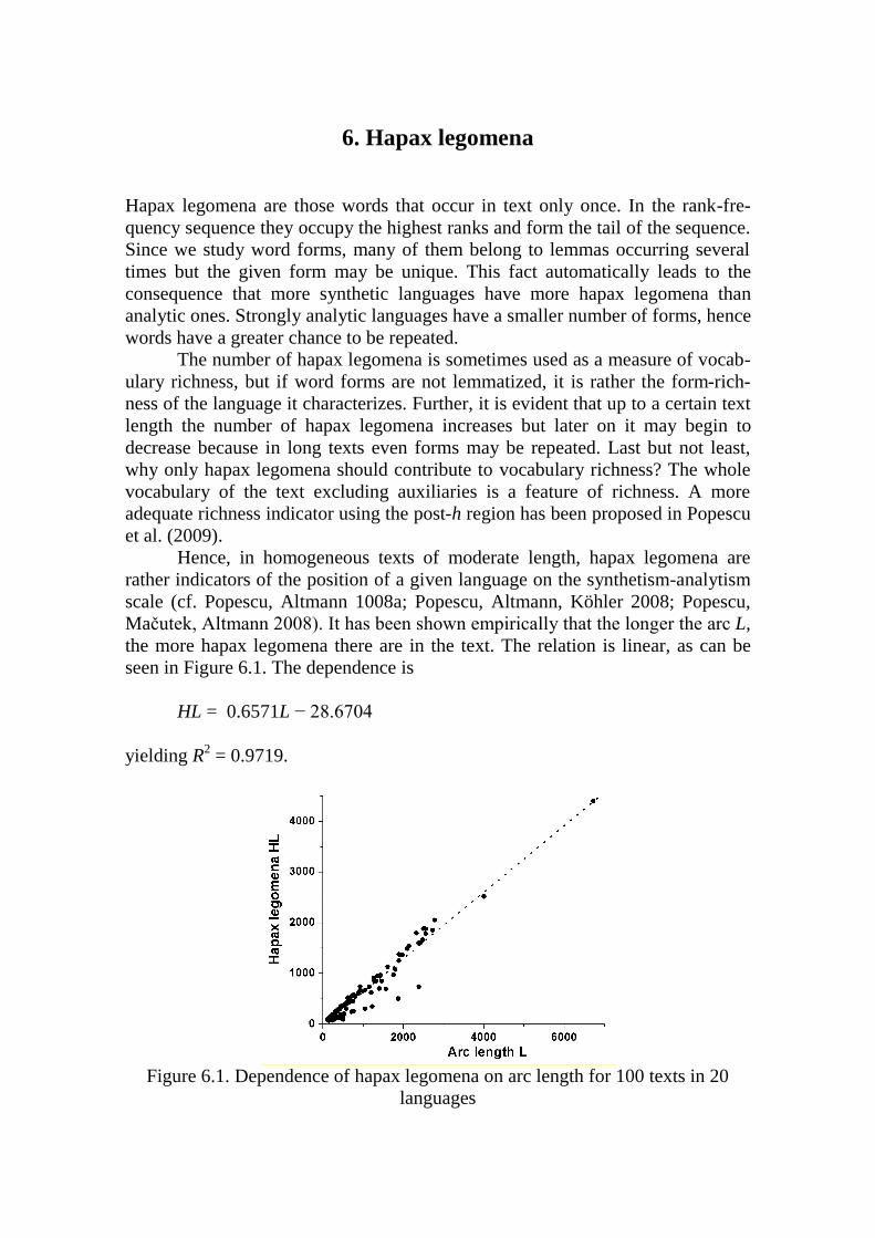
6. Hapax legomena

Hapax legomena are those words that occur in text only once. In the rank-fre-quency sequence they occupy the highest ranks and form the tail of the sequence. Since we study word forms, many of them belong to lemmas occurring several times but the given form may be unique. This fact automatically leads to the consequence that more synthetic languages have more hapax legomena than analytic ones. Strongly analytic languages have a smaller number of forms, hence words have a greater chance to be repeated. The number of hapax legomena is sometimes used as a measure of vocab-ulary richness, but if word forms are not lemmatized, it is rather the form-rich-ness of the language it characterizes. Further, it is evident that up to a certain text length the number of hapax legomena increases but later on it may begin to decrease because in long texts even forms may be repeated. Last but not least, why only hapax legomena should contribute to vocabulary richness? The whole vocabulary of the text excluding auxiliaries is a feature of richness. A more adequate richness indicator using the post-h region has been proposed in Popescu et al. (2009). Hence, in homogeneous texts of moderate length, hapax legomena are rather indicators of the position of a given language on the synthetism-analytism scale (cf. Popescu, Altmann 1008a; Popescu, Altmann, Köhler 2008; Popescu, Mačutek, Altmann 2008). It has been shown empirically that the longer the arc L, the more hapax legomena there are in the text. The relation is linear, as can be seen in Figure 6.1. The dependence is HL = 0.6571L − 28.6704 yielding R2 = 0.9719.

Figure 6.1. Dependence of hapax legomena on arc length for 100 texts in 20

languages

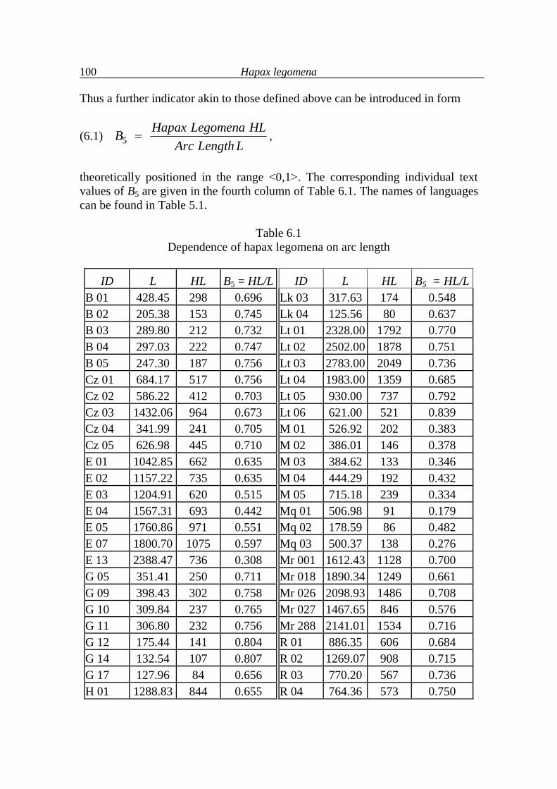
Hapax legomena

100

Thus a further indicator akin to those defined above can be introduced in form

(6.1) 5

Hapax Legomena HLB

Arc Length L ,

theoretically positioned in the range <0,1>. The corresponding individual text values of B5 are given in the fourth column of Table 6.1. The names of languages can be found in Table 5.1.

Table 6.1

Dependence of hapax legomena on arc length

ID L HL B5 = HL/L ID L HL B5 = HL/L B 01 428.45 298 0.696 Lk 03 317.63 174 0.548 B 02 205.38 153 0.745 Lk 04 125.56 80 0.637 B 03 289.80 212 0.732 Lt 01 2328.00 1792 0.770 B 04 297.03 222 0.747 Lt 02 2502.00 1878 0.751 B 05 247.30 187 0.756 Lt 03 2783.00 2049 0.736 Cz 01 684.17 517 0.756 Lt 04 1983.00 1359 0.685 Cz 02 586.22 412 0.703 Lt 05 930.00 737 0.792 Cz 03 1432.06 964 0.673 Lt 06 621.00 521 0.839 Cz 04 341.99 241 0.705 M 01 526.92 202 0.383 Cz 05 626.98 445 0.710 M 02 386.01 146 0.378 E 01 1042.85 662 0.635 M 03 384.62 133 0.346 E 02 1157.22 735 0.635 M 04 444.29 192 0.432 E 03 1204.91 620 0.515 M 05 715.18 239 0.334 E 04 1567.31 693 0.442 Mq 01 506.98 91 0.179 E 05 1760.86 971 0.551 Mq 02 178.59 86 0.482 E 07 1800.70 1075 0.597 Mq 03 500.37 138 0.276 E 13 2388.47 736 0.308 Mr 001 1612.43 1128 0.700 G 05 351.41 250 0.711 Mr 018 1890.34 1249 0.661 G 09 398.43 302 0.758 Mr 026 2098.93 1486 0.708 G 10 309.84 237 0.765 Mr 027 1467.65 846 0.576 G 11 306.80 232 0.756 Mr 288 2141.01 1534 0.716 G 12 175.44 141 0.804 R 01 886.35 606 0.684 G 14 132.54 107 0.807 R 02 1269.07 908 0.715 G 17 127.96 84 0.656 R 03 770.20 567 0.736 H 01 1288.83 844 0.655 R 04 764.36 573 0.750

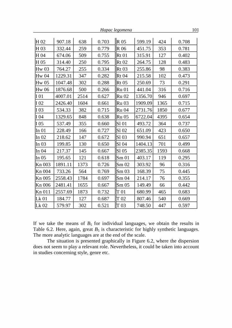
Hapac legomena

101

H 02 907.18 638 0.703 R 05 599.19 424 0.708 H 03 332.44 259 0.779 R 06 451.75 353 0.781 H 04 674.06 509 0.755 Rt 01 315.91 127 0.402 H 05 314.40 250 0.795 Rt 02 264.75 128 0.483 Hw 03 764.27 255 0.334 Rt 03 255.86 98 0.383 Hw 04 1229.31 347 0.282 Rt 04 215.58 102 0.473 Hw 05 1047.48 302 0.288 Rt 05 250.69 73 0.291 Hw 06 1876.68 500 0.266 Ru 01 441.04 316 0.716 I 01 4007.01 2514 0.627 Ru 02 1356.70 946 0.697 I 02 2426.40 1604 0.661 Ru 03 1909.09 1365 0.715 I 03 534.33 382 0.715 Ru 04 2731.76 1850 0.677 I 04 1329.65 848 0.638 Ru 05 6722.04 4395 0.654 I 05 537.49 355 0.660 Sl 01 493.72 364 0.737 In 01 228.49 166 0.727 Sl 02 651.09 423 0.650 In 02 218.62 147 0.672 Sl 03 990.94 651 0.657 In 03 199.85 130 0.650 Sl 04 1404.13 701 0.499 In 04 217.37 145 0.667 Sl 05 2385.35 1593 0.668 In 05 195.65 121 0.618 Sm 01 403.17 119 0.295 Kn 003 1891.11 1373 0.726 Sm 02 303.92 96 0.316 Kn 004 733.26 564 0.769 Sm 03 168.39 75 0.445 Kn 005 2558.43 1784 0.697 Sm 04 214.17 76 0.355 Kn 006 2481.41 1655 0.667 Sm 05 149.49 66 0.442 Kn 011 2557.69 1873 0.732 T 01 680.99 465 0.683 Lk 01 184.77 127 0.687 T 02 807.46 540 0.669 Lk 02 579.97 302 0.521 T 03 748.50 447 0.597

If we take the means of B5 for individual languages, we obtain the results in Table 6.2. Here, again, great B5 is characteristic for highly synthetic languages. The more analytic languages are at the end of the scale. The situation is presented graphically in Figure 6.2, where the dispersion does not seem to play a relevant role. Nevertheless, it could be taken into account in studies concerning style, genre etc.

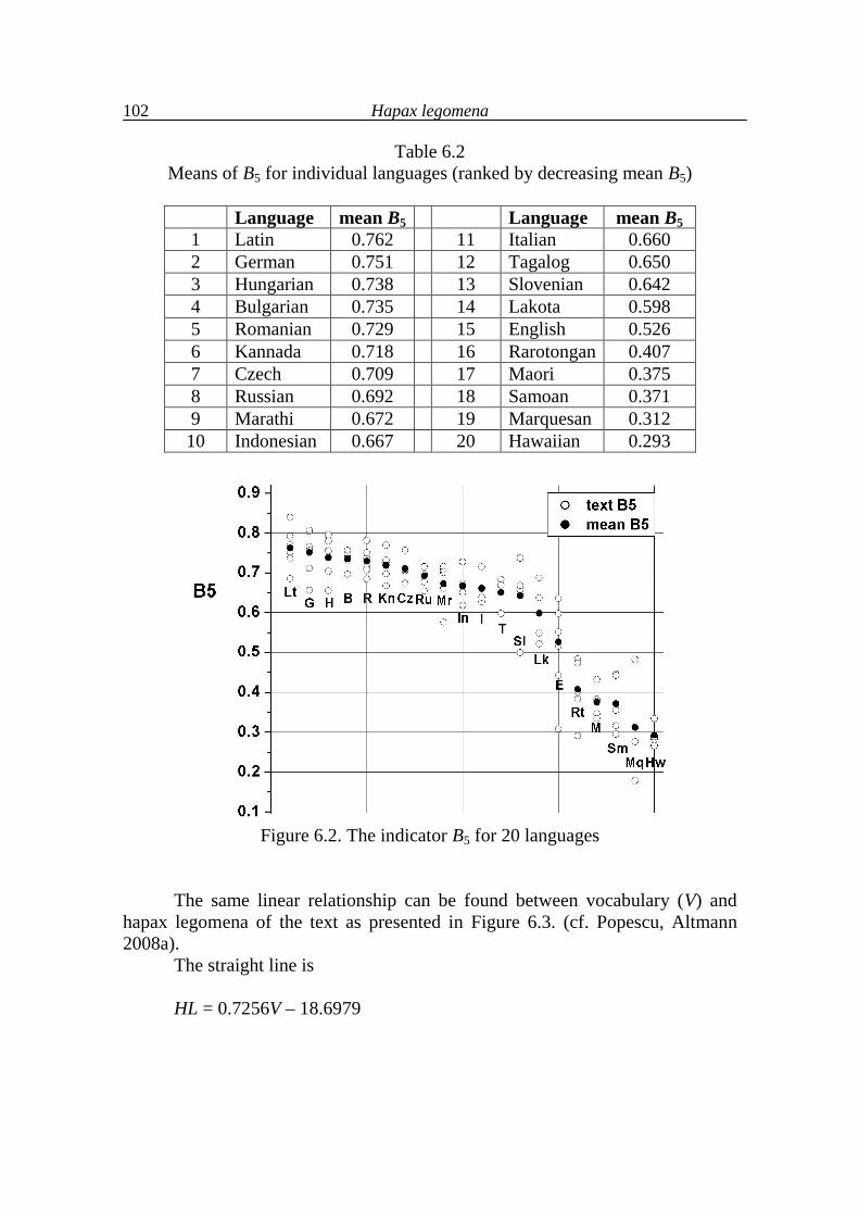
Hapax legomena

102

Table 6.2 Means of B5 for individual languages (ranked by decreasing mean B5)

Language mean B5 Language mean B5

1 Latin 0.762 11 Italian 0.660 2 German 0.751 12 Tagalog 0.650 3 Hungarian 0.738 13 Slovenian 0.642 4 Bulgarian 0.735 14 Lakota 0.598 5 Romanian 0.729 15 English 0.526 6 Kannada 0.718 16 Rarotongan 0.407 7 Czech 0.709 17 Maori 0.375 8 Russian 0.692 18 Samoan 0.371 9 Marathi 0.672 19 Marquesan 0.312

10 Indonesian 0.667 20 Hawaiian 0.293

Figure 6.2. The indicator B5 for 20 languages

The same linear relationship can be found between vocabulary (V) and hapax legomena of the text as presented in Figure 6.3. (cf. Popescu, Altmann 2008a). The straight line is HL = 0.7256V – 18.6979

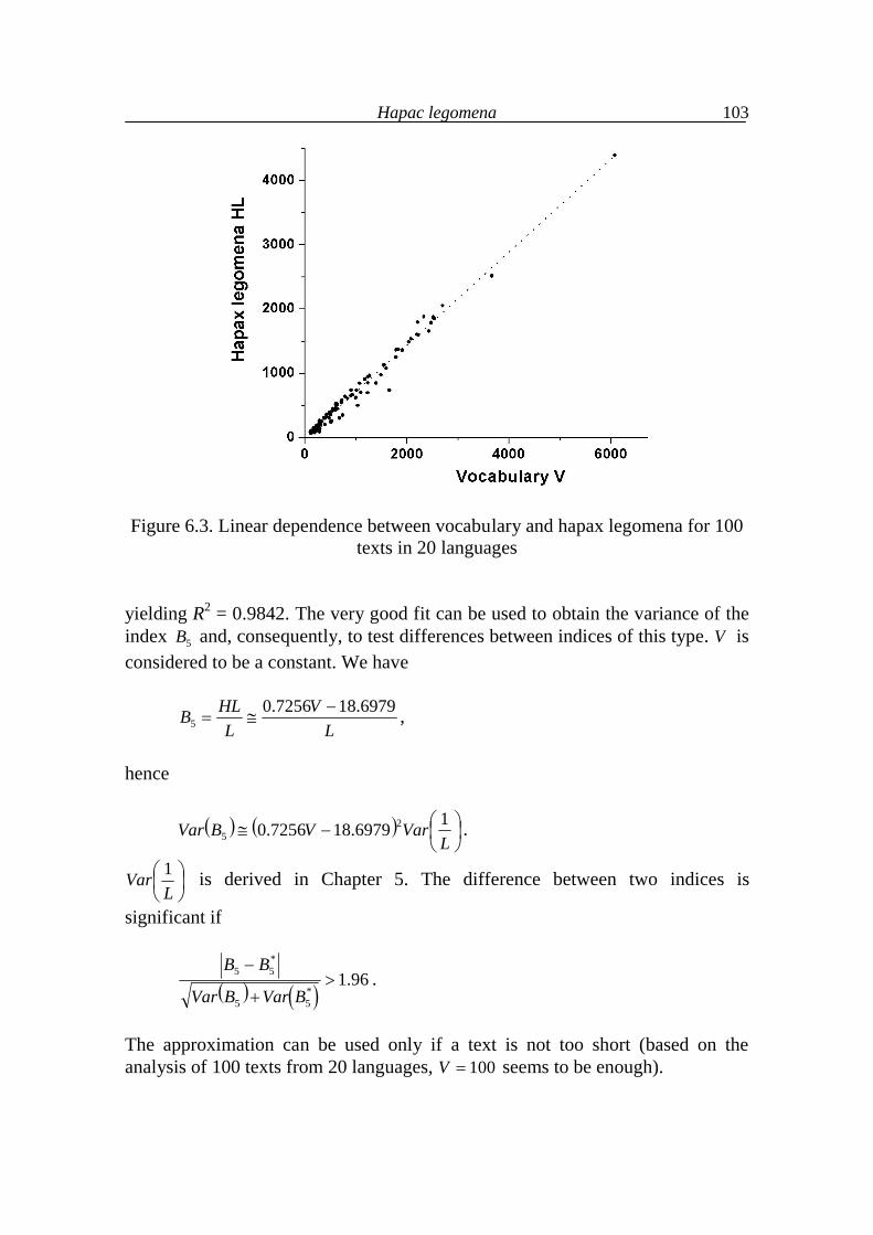
Hapac legomena

103

Figure 6.3. Linear dependence between vocabulary and hapax legomena for 100 texts in 20 languages

yielding R2 = 0.9842. The very good fit can be used to obtain the variance of the index 5B and, consequently, to test differences between indices of this type. V is considered to be a constant. We have

LV

LHLB 6979.187256.0

5

,

hence

LVarVBVar 16979.187256.0 2

5 .

LVar 1 is derived in Chapter 5. The difference between two indices is

significant if

96.1

*55

*55

BVarBVar

BB.

The approximation can be used only if a text is not too short (based on the analysis of 100 texts from 20 languages, 100V seems to be enough).

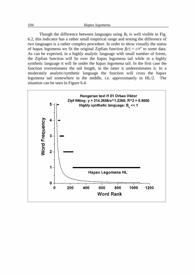
Hapax legomena

104

Though the difference between languages using B5 is well visible in Fig. 6.2, this indicator has a rather small empirical range and testing the difference of two languages is a rather complex procedure. In order to show visually the status of hapax legomena we fit the original Zipfian function f(r) = c/ra to some data. As can be expected, in a highly analytic language with small number of forms, the Zipfian function will lie over the hapax legomena tail while in a highly synthetic language it will lie under the hapax legomena tail. In the first case the function overestimates the tail length, in the latter it underestimates it. In a moderately analytic/synthetic language the function will cross the hapax legomena tail somewhere in the middle, i.e. approximately in HL/2. The situation can be seen in Figure 6.4.

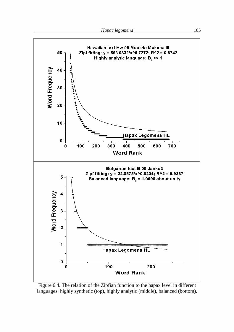
Hapac legomena

105

Figure 6.4. The relation of the Zipfian function to the hapax level in different languages: highly synthetic (top), highly analytic (middle), balanced (bottom).

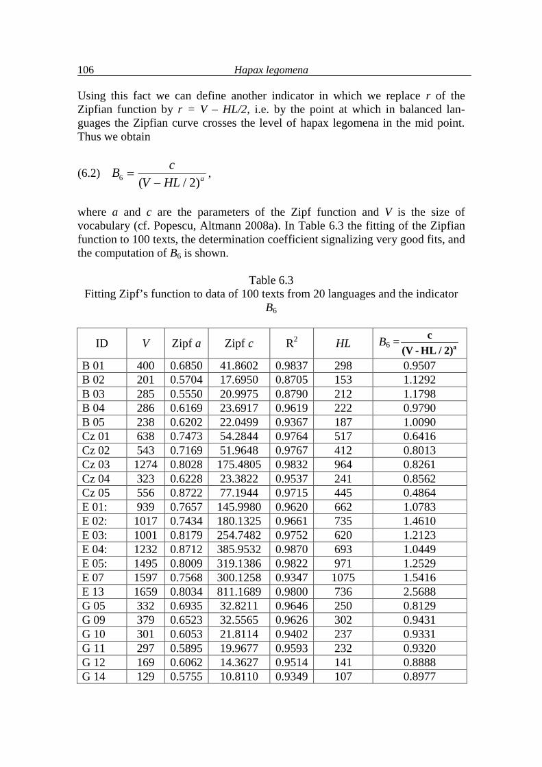
Hapax legomena

106

Using this fact we can define another indicator in which we replace r of the Zipfian function by r = V – HL/2, i.e. by the point at which in balanced lan-guages the Zipfian curve crosses the level of hapax legomena in the mid point. Thus we obtain

(6.2) 6 ( / 2)acB

V HL

,

where a and c are the parameters of the Zipf function and V is the size of vocabulary (cf. Popescu, Altmann 2008a). In Table 6.3 the fitting of the Zipfian function to 100 texts, the determination coefficient signalizing very good fits, and the computation of B6 is shown.

Table 6.3 Fitting Zipf’s function to data of 100 texts from 20 languages and the indicator

B6

ID V Zipf a Zipf c R2 HL B6 = a

c(V - HL / 2)

B 01 400 0.6850 41.8602 0.9837 298 0.9507 B 02 201 0.5704 17.6950 0.8705 153 1.1292 B 03 285 0.5550 20.9975 0.8790 212 1.1798 B 04 286 0.6169 23.6917 0.9619 222 0.9790 B 05 238 0.6202 22.0499 0.9367 187 1.0090 Cz 01 638 0.7473 54.2844 0.9764 517 0.6416 Cz 02 543 0.7169 51.9648 0.9767 412 0.8013 Cz 03 1274 0.8028 175.4805 0.9832 964 0.8261 Cz 04 323 0.6228 23.3822 0.9537 241 0.8562 Cz 05 556 0.8722 77.1944 0.9715 445 0.4864 E 01: 939 0.7657 145.9980 0.9620 662 1.0783 E 02: 1017 0.7434 180.1325 0.9661 735 1.4610 E 03: 1001 0.8179 254.7482 0.9752 620 1.2123 E 04: 1232 0.8712 385.9532 0.9870 693 1.0449 E 05: 1495 0.8009 319.1386 0.9822 971 1.2529 E 07 1597 0.7568 300.1258 0.9347 1075 1.5416 E 13 1659 0.8034 811.1689 0.9800 736 2.5688 G 05 332 0.6935 32.8211 0.9646 250 0.8129 G 09 379 0.6523 32.5565 0.9626 302 0.9431 G 10 301 0.6053 21.8114 0.9402 237 0.9331 G 11 297 0.5895 19.9677 0.9593 232 0.9320 G 12 169 0.6062 14.3627 0.9514 141 0.8888 G 14 129 0.5755 10.8110 0.9349 107 0.8977

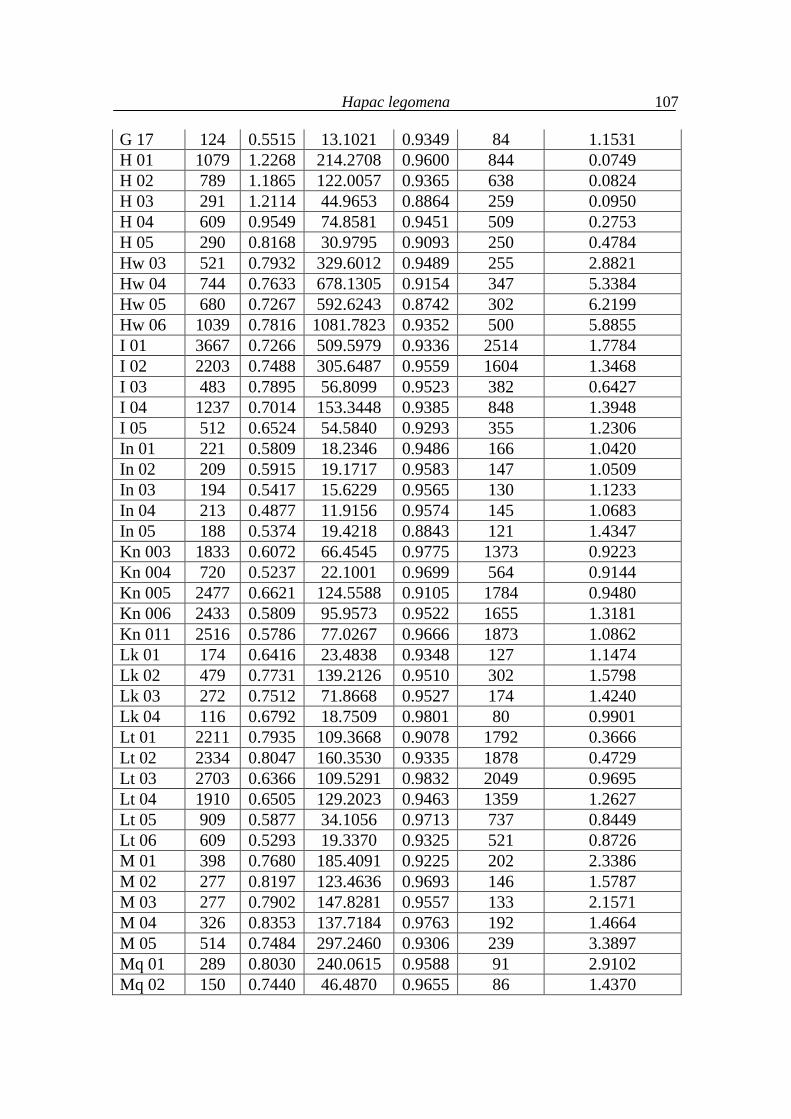
Hapac legomena

107

G 17 124 0.5515 13.1021 0.9349 84 1.1531 H 01 1079 1.2268 214.2708 0.9600 844 0.0749 H 02 789 1.1865 122.0057 0.9365 638 0.0824 H 03 291 1.2114 44.9653 0.8864 259 0.0950 H 04 609 0.9549 74.8581 0.9451 509 0.2753 H 05 290 0.8168 30.9795 0.9093 250 0.4784 Hw 03 521 0.7932 329.6012 0.9489 255 2.8821 Hw 04 744 0.7633 678.1305 0.9154 347 5.3384 Hw 05 680 0.7267 592.6243 0.8742 302 6.2199 Hw 06 1039 0.7816 1081.7823 0.9352 500 5.8855 I 01 3667 0.7266 509.5979 0.9336 2514 1.7784 I 02 2203 0.7488 305.6487 0.9559 1604 1.3468 I 03 483 0.7895 56.8099 0.9523 382 0.6427 I 04 1237 0.7014 153.3448 0.9385 848 1.3948 I 05 512 0.6524 54.5840 0.9293 355 1.2306 In 01 221 0.5809 18.2346 0.9486 166 1.0420 In 02 209 0.5915 19.1717 0.9583 147 1.0509 In 03 194 0.5417 15.6229 0.9565 130 1.1233 In 04 213 0.4877 11.9156 0.9574 145 1.0683 In 05 188 0.5374 19.4218 0.8843 121 1.4347 Kn 003 1833 0.6072 66.4545 0.9775 1373 0.9223 Kn 004 720 0.5237 22.1001 0.9699 564 0.9144 Kn 005 2477 0.6621 124.5588 0.9105 1784 0.9480 Kn 006 2433 0.5809 95.9573 0.9522 1655 1.3181 Kn 011 2516 0.5786 77.0267 0.9666 1873 1.0862 Lk 01 174 0.6416 23.4838 0.9348 127 1.1474 Lk 02 479 0.7731 139.2126 0.9510 302 1.5798 Lk 03 272 0.7512 71.8668 0.9527 174 1.4240 Lk 04 116 0.6792 18.7509 0.9801 80 0.9901 Lt 01 2211 0.7935 109.3668 0.9078 1792 0.3666 Lt 02 2334 0.8047 160.3530 0.9335 1878 0.4729 Lt 03 2703 0.6366 109.5291 0.9832 2049 0.9695 Lt 04 1910 0.6505 129.2023 0.9463 1359 1.2627 Lt 05 909 0.5877 34.1056 0.9713 737 0.8449 Lt 06 609 0.5293 19.3370 0.9325 521 0.8726 M 01 398 0.7680 185.4091 0.9225 202 2.3386 M 02 277 0.8197 123.4636 0.9693 146 1.5787 M 03 277 0.7902 147.8281 0.9557 133 2.1571 M 04 326 0.8353 137.7184 0.9763 192 1.4664 M 05 514 0.7484 297.2460 0.9306 239 3.3897 Mq 01 289 0.8030 240.0615 0.9588 91 2.9102 Mq 02 150 0.7440 46.4870 0.9655 86 1.4370

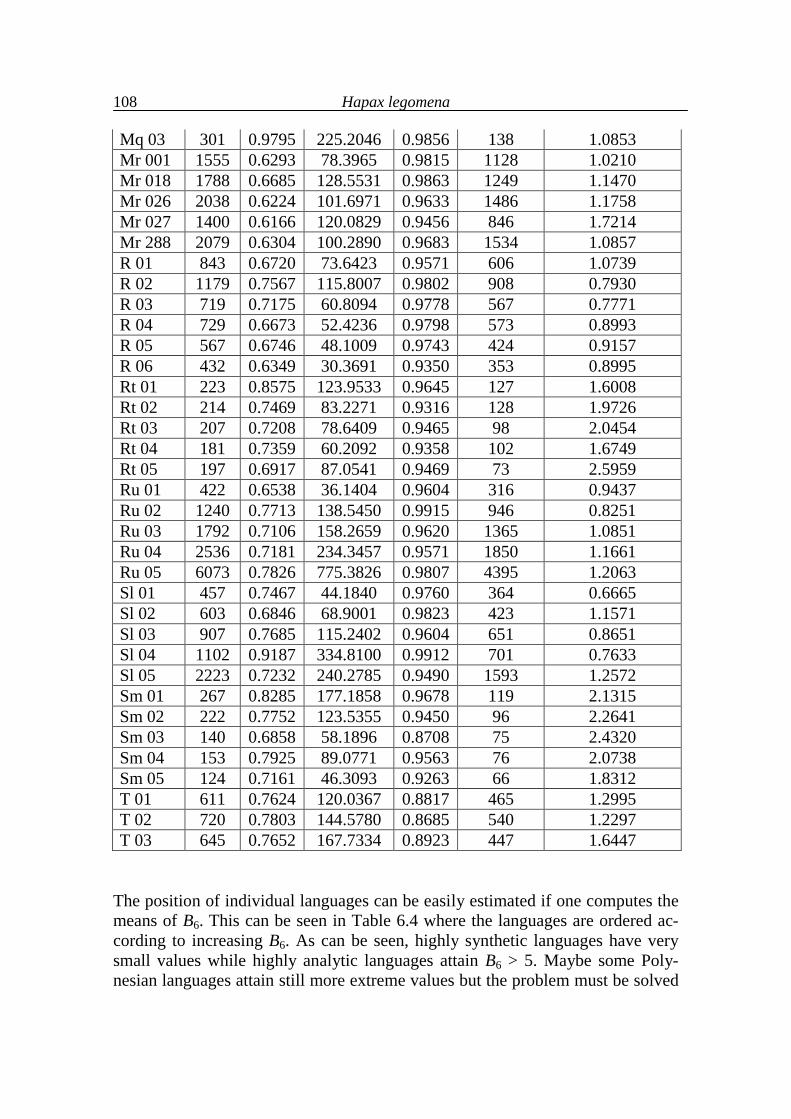
Hapax legomena

108

Mq 03 301 0.9795 225.2046 0.9856 138 1.0853 Mr 001 1555 0.6293 78.3965 0.9815 1128 1.0210 Mr 018 1788 0.6685 128.5531 0.9863 1249 1.1470 Mr 026 2038 0.6224 101.6971 0.9633 1486 1.1758 Mr 027 1400 0.6166 120.0829 0.9456 846 1.7214 Mr 288 2079 0.6304 100.2890 0.9683 1534 1.0857 R 01 843 0.6720 73.6423 0.9571 606 1.0739 R 02 1179 0.7567 115.8007 0.9802 908 0.7930 R 03 719 0.7175 60.8094 0.9778 567 0.7771 R 04 729 0.6673 52.4236 0.9798 573 0.8993 R 05 567 0.6746 48.1009 0.9743 424 0.9157 R 06 432 0.6349 30.3691 0.9350 353 0.8995 Rt 01 223 0.8575 123.9533 0.9645 127 1.6008 Rt 02 214 0.7469 83.2271 0.9316 128 1.9726 Rt 03 207 0.7208 78.6409 0.9465 98 2.0454 Rt 04 181 0.7359 60.2092 0.9358 102 1.6749 Rt 05 197 0.6917 87.0541 0.9469 73 2.5959 Ru 01 422 0.6538 36.1404 0.9604 316 0.9437 Ru 02 1240 0.7713 138.5450 0.9915 946 0.8251 Ru 03 1792 0.7106 158.2659 0.9620 1365 1.0851 Ru 04 2536 0.7181 234.3457 0.9571 1850 1.1661 Ru 05 6073 0.7826 775.3826 0.9807 4395 1.2063 Sl 01 457 0.7467 44.1840 0.9760 364 0.6665 Sl 02 603 0.6846 68.9001 0.9823 423 1.1571 Sl 03 907 0.7685 115.2402 0.9604 651 0.8651 Sl 04 1102 0.9187 334.8100 0.9912 701 0.7633 Sl 05 2223 0.7232 240.2785 0.9490 1593 1.2572 Sm 01 267 0.8285 177.1858 0.9678 119 2.1315 Sm 02 222 0.7752 123.5355 0.9450 96 2.2641 Sm 03 140 0.6858 58.1896 0.8708 75 2.4320 Sm 04 153 0.7925 89.0771 0.9563 76 2.0738 Sm 05 124 0.7161 46.3093 0.9263 66 1.8312 T 01 611 0.7624 120.0367 0.8817 465 1.2995 T 02 720 0.7803 144.5780 0.8685 540 1.2297 T 03 645 0.7652 167.7334 0.8923 447 1.6447

The position of individual languages can be easily estimated if one computes the means of B6. This can be seen in Table 6.4 where the languages are ordered ac-cording to increasing B6. As can be seen, highly synthetic languages have very small values while highly analytic languages attain B6 > 5. Maybe some Poly-nesian languages attain still more extreme values but the problem must be solved

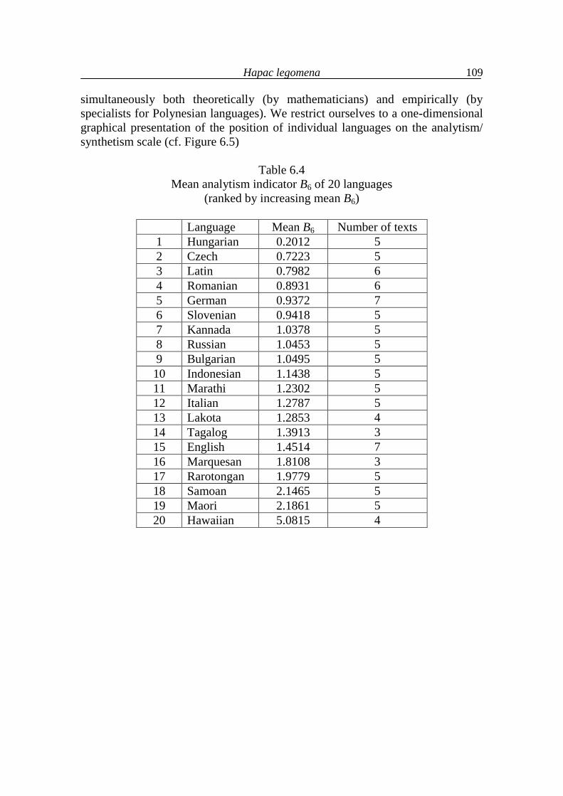
Hapac legomena

109

simultaneously both theoretically (by mathematicians) and empirically (by specialists for Polynesian languages). We restrict ourselves to a one-dimensional graphical presentation of the position of individual languages on the analytism/ synthetism scale (cf. Figure 6.5)

Table 6.4 Mean analytism indicator B6 of 20 languages

(ranked by increasing mean B6)

Language Mean B6 Number of texts 1 Hungarian 0.2012 5 2 Czech 0.7223 5 3 Latin 0.7982 6 4 Romanian 0.8931 6 5 German 0.9372 7 6 Slovenian 0.9418 5 7 Kannada 1.0378 5 8 Russian 1.0453 5 9 Bulgarian 1.0495 5

10 Indonesian 1.1438 5 11 Marathi 1.2302 5 12 Italian 1.2787 5 13 Lakota 1.2853 4 14 Tagalog 1.3913 3 15 English 1.4514 7 16 Marquesan 1.8108 3 17 Rarotongan 1.9779 5 18 Samoan 2.1465 5 19 Maori 2.1861 5 20 Hawaiian 5.0815 4

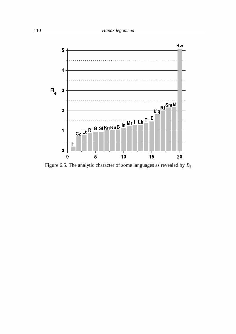
Hapax legomena

110

Figure 6.5. The analytic character of some languages as revealed by B6

7. Further typological considerations

Though for fitting purposes we abandoned Zipf´s (zeta) function and replaced it by a sum of exponentials, the function demonstrated its utility in typological con-siderations. But the typology of languages is an analogy to text typology in in-dividual languages, e.g. associated with style, genre etc., hence all results of typological studies of a language can be transferred into the study of texts in a given language. This task can be left to specialized philologists; here it is dealt with in a general way. As has been shown in Chapter 6, for highly analytic languages Zipf´s function lies over the hapax legomena; the contrary holds for highly synthetic languages. In the first case it means that the empirical average defined as

(7.1) 1

1 ( )V

Er

M rf rN

,

where N is text length, V is the vocabulary, r the rank and f(r) the frequency at rank r, must be much smaller than the average MZ computed using the Zipfian f(r) = c/ra inserted in (7.1). The parameters c and a must be computed iteratively. On the contrary, in highly synthetic languages the empirical mean will be greater than the Zipfian. In order to express the difference, we define the indicator (cf. Popescu, Altmann 2008b)

(7.2) 7E Z

E

M MBM

,

which can be interpreted as follows: if B7 > 0, then the language tends to synthetism if B7 < 0, then the language tends to analytism if B7 ≈ 0, then the language is balanced and contains both kinds of phenomena. As an example let us consider the frequency count of word forms in the Hawaiian text Hw 05 Moolelo Mokuna III (also presented in Figure 6.4). The empirical text size and mean yield N = 7620 and ME = 68.7388. Now, using the Zipfian iterative fitting f(r) = c/ra, we obtain the function f(r) = 592.6243r−0.7267. Its text size (the integral of f(r) from 1 to V) and mean yield NZ = 11056.8403 and MZ = 170.3493. Inserting these two means in (7.2) we obtain

B7 (Hw 05) = 68.7388 – 170.3493

68.7388 = -1.4782,

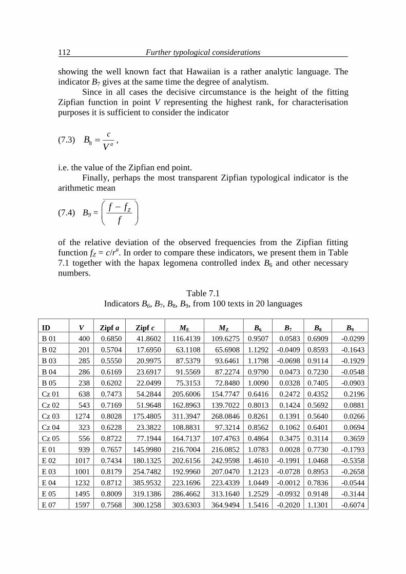
Further typological considerations

112

showing the well known fact that Hawaiian is a rather analytic language. The indicator B7 gives at the same time the degree of analytism. Since in all cases the decisive circumstance is the height of the fitting Zipfian function in point V representing the highest rank, for characterisation purposes it is sufficient to consider the indicator

(7.3) 8 a

cBV

,

i.e. the value of the Zipfian end point. Finally, perhaps the most transparent Zipfian typological indicator is the arithmetic mean

(7.4) B9 =

____________

Zf ff

of the relative deviation of the observed frequencies from the Zipfian fitting function fZ = c/ra. In order to compare these indicators, we present them in Table 7.1 together with the hapax legomena controlled index B6 and other necessary numbers.

Table 7.1 Indicators B6, B7, B8, B9, from 100 texts in 20 languages

ID V Zipf a Zipf c ME MZ B6 B7 B8 B9 B 01 400 0.6850 41.8602 116.4139 109.6275 0.9507 0.0583 0.6909 -0.0299 B 02 201 0.5704 17.6950 63.1108 65.6908 1.1292 -0.0409 0.8593 -0.1643 B 03 285 0.5550 20.9975 87.5379 93.6461 1.1798 -0.0698 0.9114 -0.1929 B 04 286 0.6169 23.6917 91.5569 87.2274 0.9790 0.0473 0.7230 -0.0548 B 05 238 0.6202 22.0499 75.3153 72.8480 1.0090 0.0328 0.7405 -0.0903 Cz 01 638 0.7473 54.2844 205.6006 154.7747 0.6416 0.2472 0.4352 0.2196 Cz 02 543 0.7169 51.9648 162.8963 139.7022 0.8013 0.1424 0.5692 0.0881 Cz 03 1274 0.8028 175.4805 311.3947 268.0846 0.8261 0.1391 0.5640 0.0266 Cz 04 323 0.6228 23.3822 108.8831 97.3214 0.8562 0.1062 0.6401 0.0694 Cz 05 556 0.8722 77.1944 164.7137 107.4763 0.4864 0.3475 0.3114 0.3659 E 01 939 0.7657 145.9980 216.7004 216.0852 1.0783 0.0028 0.7730 -0.1793 E 02 1017 0.7434 180.1325 202.6156 242.9598 1.4610 -0.1991 1.0468 -0.5358 E 03 1001 0.8179 254.7482 192.9960 207.0470 1.2123 -0.0728 0.8953 -0.2658 E 04 1232 0.8712 385.9532 223.1696 223.4339 1.0449 -0.0012 0.7836 -0.0544 E 05 1495 0.8009 319.1386 286.4662 313.1640 1.2529 -0.0932 0.9148 -0.3144 E 07 1597 0.7568 300.1258 303.6303 364.9494 1.5416 -0.2020 1.1301 -0.6074

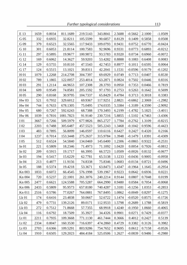
Further typological considerations

113

E 13 1659 0.8034 811.1689 219.5143 343.8041 2.5688 -0.5662 2.1000 -1.0509 G 05 332 0.6935 32.8211 105.5599 90.6857 0.8129 0.1409 0.5858 0.0508 G 09 379 0.6523 32.5565 117.9433 109.0793 0.9431 0.0752 0.6770 -0.0424 G 10 301 0.6053 21.8114 100.7583 92.9696 0.9331 0.0773 0.6893 -0.0212 G 11 297 0.5895 19.9677 100.9872 93.5783 0.9320 0.0734 0.6960 -0.0072 G 12 169 0.6062 14.3627 59.9203 53.4282 0.8888 0.1083 0.6408 0.0083 G 14 129 0.5755 10.8110 47.5543 42.7453 0.8977 0.1011 0.6595 0.0064 G 17 124 0.5515 13.1021 39.8311 42.2041 1.1531 -0.0596 0.9179 -0.1202 H 01 1079 1.2268 214.2708 304.7397 69.6929 0.0749 0.7713 0.0407 0.8530 H 02 789 1.1865 122.0057 253.4014 63.2871 0.0824 0.7502 0.0446 0.8316 H 03 291 1.2114 44.9653 107.2308 28.3793 0.0950 0.7353 0.0466 0.7819 H 04 609 0.9549 74.8581 205.1592 97.1793 0.2753 0.5263 0.1642 0.5699 H 05 290 0.8168 30.9795 104.7337 65.8429 0.4784 0.3713 0.3018 0.3383 Hw 03 521 0.7932 329.6012 69.9367 117.9251 2.8821 -0.6862 2.3069 -1.2982 Hw 04 744 0.7633 678.1305 75.0495 174.0335 5.3384 -1.3189 4.3590 -2.9092 Hw 05 680 0.7267 592.6243 68.7388 170.3493 6.2199 -1.4782 5.1825 -3.4011 Hw 06 1039 0.7816 1081.7823 91.9140 230.7216 5.8855 -1.5102 4.7463 -3.4306 I 01 3667 0.7266 509.5979 677.9826 865.2727 1.7784 -0.2762 1.3109 -0.8215 I 02 2203 0.7488 305.6487 457.5523 505.2243 1.3468 -0.1042 0.9596 -0.4423 I 03 483 0.7895 56.8099 146.0597 110.6116 0.6427 0.2427 0.4320 0.2166 I 04 1237 0.7014 153.3448 275.2637 315.9784 1.3948 -0.1479 1.0391 -0.4309 I 05 512 0.6524 54.5840 134.0469 145.6400 1.2306 -0.0865 0.9322 -0.2531 In 01 221 0.5809 18.2346 71.4973 71.1092 1.0420 0.0054 0.7926 -0.0812 In 02 209 0.5915 19.1717 66.3995 66.5723 1.0509 -0.0026 0.8132 -0.0677 In 03 194 0.5417 15.6229 62.7781 65.5138 1.1233 -0.0436 0.9005 -0.0958 In 04 213 0.4877 11.9156 74.8338 75.8346 1.0683 -0.0134 0.8721 -0.0496 In 05 188 0.5374 19.4218 53.3671 63.8473 1.4347 -0.1964 1.1645 -0.2954 Kn 003 1833 0.6072 66.4545 576.1998 539.1967 0.9223 0.0642 0.6936 0.0221 Kn 004 720 0.5237 22.1001 261.3076 240.2214 0.9144 0.0807 0.7048 0.0199 Kn 005 2477 0.6621 124.5588 705.5287 664.2990 0.9480 0.0584 0.7054 -0.0068 Kn 006 2433 0.5809 95.9573 657.8180 740.4287 1.3181 -0.1256 1.0353 -0.2853 Kn 011 2516 0.5786 77.0267 764.0881 767.8495 1.0862 -0.0049 0.8297 -0.1275 Lk 01 174 0.6416 23.4838 50.0667 52.6722 1.1474 -0.0520 0.8575 -0.1726 Lk 02 479 0.7731 139.2126 89.0171 112.9533 1.5798 -0.2689 1.1788 -0.5819 Lk 03 272 0.7512 71.8668 57.7355 68.9918 1.4240 -0.1950 1.0660 -0.4065 Lk 04 116 0.6792 18.7509 35.3927 34.4326 0.9901 0.0271 0.7429 -0.0377 Lt 01 2211 0.7935 109.3668 771.1130 461.7444 0.3666 0.4012 0.2427 0.5139 Lt 02 2334 0.8047 160.3530 716.6397 474.2860 0.4729 0.3382 0.3126 0.3982 Lt 03 2703 0.6366 109.5291 803.9286 754.7652 0.9695 0.0612 0.7158 -0.0526 Lt 04 1910 0.6505 129.2023 484.4184 525.0506 1.2627 -0.0839 0.9486 -0.2980

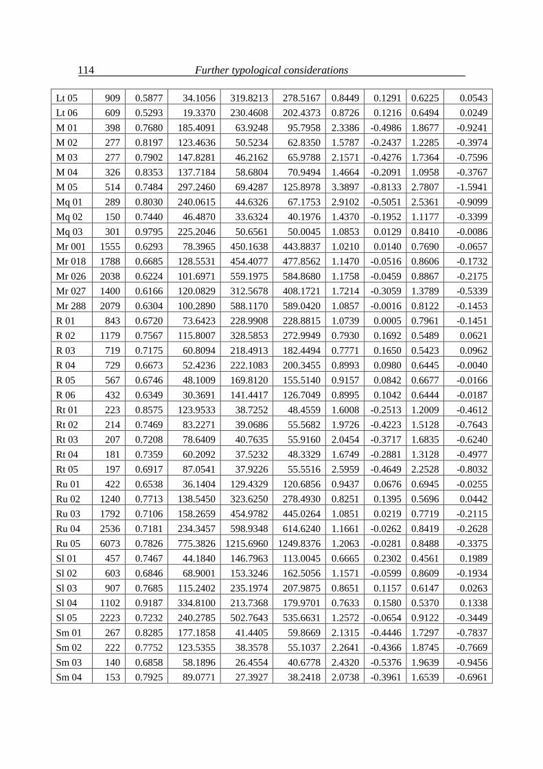
Further typological considerations

114

Lt 05 909 0.5877 34.1056 319.8213 278.5167 0.8449 0.1291 0.6225 0.0543 Lt 06 609 0.5293 19.3370 230.4608 202.4373 0.8726 0.1216 0.6494 0.0249 M 01 398 0.7680 185.4091 63.9248 95.7958 2.3386 -0.4986 1.8677 -0.9241 M 02 277 0.8197 123.4636 50.5234 62.8350 1.5787 -0.2437 1.2285 -0.3974 M 03 277 0.7902 147.8281 46.2162 65.9788 2.1571 -0.4276 1.7364 -0.7596 M 04 326 0.8353 137.7184 58.6804 70.9494 1.4664 -0.2091 1.0958 -0.3767 M 05 514 0.7484 297.2460 69.4287 125.8978 3.3897 -0.8133 2.7807 -1.5941 Mq 01 289 0.8030 240.0615 44.6326 67.1753 2.9102 -0.5051 2.5361 -0.9099 Mq 02 150 0.7440 46.4870 33.6324 40.1976 1.4370 -0.1952 1.1177 -0.3399 Mq 03 301 0.9795 225.2046 50.6561 50.0045 1.0853 0.0129 0.8410 -0.0086 Mr 001 1555 0.6293 78.3965 450.1638 443.8837 1.0210 0.0140 0.7690 -0.0657 Mr 018 1788 0.6685 128.5531 454.4077 477.8562 1.1470 -0.0516 0.8606 -0.1732 Mr 026 2038 0.6224 101.6971 559.1975 584.8680 1.1758 -0.0459 0.8867 -0.2175 Mr 027 1400 0.6166 120.0829 312.5678 408.1721 1.7214 -0.3059 1.3789 -0.5339 Mr 288 2079 0.6304 100.2890 588.1170 589.0420 1.0857 -0.0016 0.8122 -0.1453 R 01 843 0.6720 73.6423 228.9908 228.8815 1.0739 0.0005 0.7961 -0.1451 R 02 1179 0.7567 115.8007 328.5853 272.9949 0.7930 0.1692 0.5489 0.0621 R 03 719 0.7175 60.8094 218.4913 182.4494 0.7771 0.1650 0.5423 0.0962 R 04 729 0.6673 52.4236 222.1083 200.3455 0.8993 0.0980 0.6445 -0.0040 R 05 567 0.6746 48.1009 169.8120 155.5140 0.9157 0.0842 0.6677 -0.0166 R 06 432 0.6349 30.3691 141.4417 126.7049 0.8995 0.1042 0.6444 -0.0187 Rt 01 223 0.8575 123.9533 38.7252 48.4559 1.6008 -0.2513 1.2009 -0.4612 Rt 02 214 0.7469 83.2271 39.0686 55.5682 1.9726 -0.4223 1.5128 -0.7643 Rt 03 207 0.7208 78.6409 40.7635 55.9160 2.0454 -0.3717 1.6835 -0.6240 Rt 04 181 0.7359 60.2092 37.5232 48.3329 1.6749 -0.2881 1.3128 -0.4977 Rt 05 197 0.6917 87.0541 37.9226 55.5516 2.5959 -0.4649 2.2528 -0.8032 Ru 01 422 0.6538 36.1404 129.4329 120.6856 0.9437 0.0676 0.6945 -0.0255 Ru 02 1240 0.7713 138.5450 323.6250 278.4930 0.8251 0.1395 0.5696 0.0442 Ru 03 1792 0.7106 158.2659 454.9782 445.0264 1.0851 0.0219 0.7719 -0.2115 Ru 04 2536 0.7181 234.3457 598.9348 614.6240 1.1661 -0.0262 0.8419 -0.2628 Ru 05 6073 0.7826 775.3826 1215.6960 1249.8376 1.2063 -0.0281 0.8488 -0.3375 Sl 01 457 0.7467 44.1840 146.7963 113.0045 0.6665 0.2302 0.4561 0.1989 Sl 02 603 0.6846 68.9001 153.3246 162.5056 1.1571 -0.0599 0.8609 -0.1934 Sl 03 907 0.7685 115.2402 235.1974 207.9875 0.8651 0.1157 0.6147 0.0263 Sl 04 1102 0.9187 334.8100 213.7368 179.9701 0.7633 0.1580 0.5370 0.1338 Sl 05 2223 0.7232 240.2785 502.7643 535.6631 1.2572 -0.0654 0.9122 -0.3449 Sm 01 267 0.8285 177.1858 41.4405 59.8669 2.1315 -0.4446 1.7297 -0.7837 Sm 02 222 0.7752 123.5355 38.3578 55.1037 2.2641 -0.4366 1.8745 -0.7669 Sm 03 140 0.6858 58.1896 26.4554 40.6778 2.4320 -0.5376 1.9639 -0.9456 Sm 04 153 0.7925 89.0771 27.3927 38.2418 2.0738 -0.3961 1.6539 -0.6961

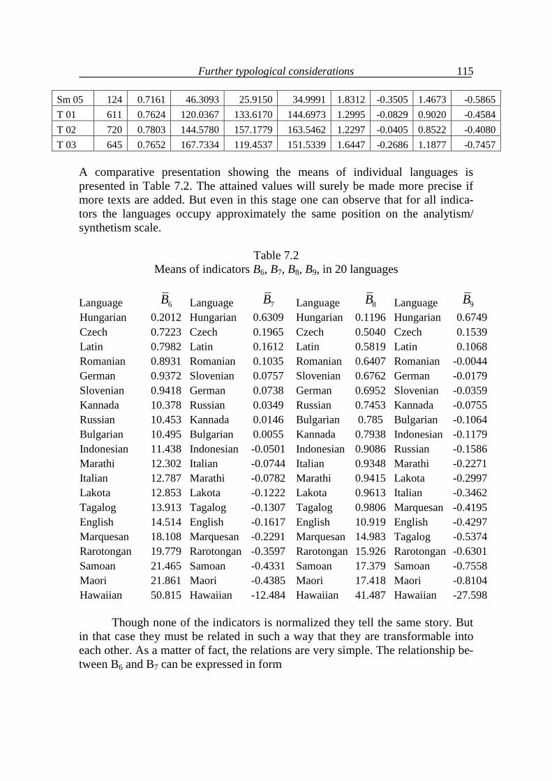
Further typological considerations

115

Sm 05 124 0.7161 46.3093 25.9150 34.9991 1.8312 -0.3505 1.4673 -0.5865 T 01 611 0.7624 120.0367 133.6170 144.6973 1.2995 -0.0829 0.9020 -0.4584 T 02 720 0.7803 144.5780 157.1779 163.5462 1.2297 -0.0405 0.8522 -0.4080 T 03 645 0.7652 167.7334 119.4537 151.5339 1.6447 -0.2686 1.1877 -0.7457

A comparative presentation showing the means of individual languages is presented in Table 7.2. The attained values will surely be made more precise if more texts are added. But even in this stage one can observe that for all indica-tors the languages occupy approximately the same position on the analytism/ synthetism scale.

Table 7.2 Means of indicators B6, B7, B8, B9, in 20 languages

Language 6B Language 7B Language 8B Language 9B Hungarian 0.2012 Hungarian 0.6309 Hungarian 0.1196 Hungarian 0.6749 Czech 0.7223 Czech 0.1965 Czech 0.5040 Czech 0.1539 Latin 0.7982 Latin 0.1612 Latin 0.5819 Latin 0.1068 Romanian 0.8931 Romanian 0.1035 Romanian 0.6407 Romanian -0.0044 German 0.9372 Slovenian 0.0757 Slovenian 0.6762 German -0.0179 Slovenian 0.9418 German 0.0738 German 0.6952 Slovenian -0.0359 Kannada 10.378 Russian 0.0349 Russian 0.7453 Kannada -0.0755 Russian 10.453 Kannada 0.0146 Bulgarian 0.785 Bulgarian -0.1064 Bulgarian 10.495 Bulgarian 0.0055 Kannada 0.7938 Indonesian -0.1179 Indonesian 11.438 Indonesian -0.0501 Indonesian 0.9086 Russian -0.1586 Marathi 12.302 Italian -0.0744 Italian 0.9348 Marathi -0.2271 Italian 12.787 Marathi -0.0782 Marathi 0.9415 Lakota -0.2997 Lakota 12.853 Lakota -0.1222 Lakota 0.9613 Italian -0.3462 Tagalog 13.913 Tagalog -0.1307 Tagalog 0.9806 Marquesan -0.4195 English 14.514 English -0.1617 English 10.919 English -0.4297 Marquesan 18.108 Marquesan -0.2291 Marquesan 14.983 Tagalog -0.5374 Rarotongan 19.779 Rarotongan -0.3597 Rarotongan 15.926 Rarotongan -0.6301 Samoan 21.465 Samoan -0.4331 Samoan 17.379 Samoan -0.7558 Maori 21.861 Maori -0.4385 Maori 17.418 Maori -0.8104 Hawaiian 50.815 Hawaiian -12.484 Hawaiian 41.487 Hawaiian -27.598

Though none of the indicators is normalized they tell the same story. But in that case they must be related in such a way that they are transformable into each other. As a matter of fact, the relations are very simple. The relationship be-tween B6 and B7 can be expressed in form

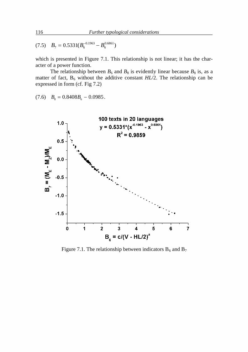
Further typological considerations

116

(7.5) 0.1963 0.68617 6 60.5331( )B B B

which is presented in Figure 7.1. This relationship is not linear; it has the char-acter of a power function. The relationship between B6 and B8 is evidently linear because B8 is, as a matter of fact, B6 without the additive constant HL/2. The relationship can be expressed in form (cf. Fig 7.2) (7.6) 8 60.8408 0.0985B B .

Figure 7.1. The relationship between indicators B6 and B7

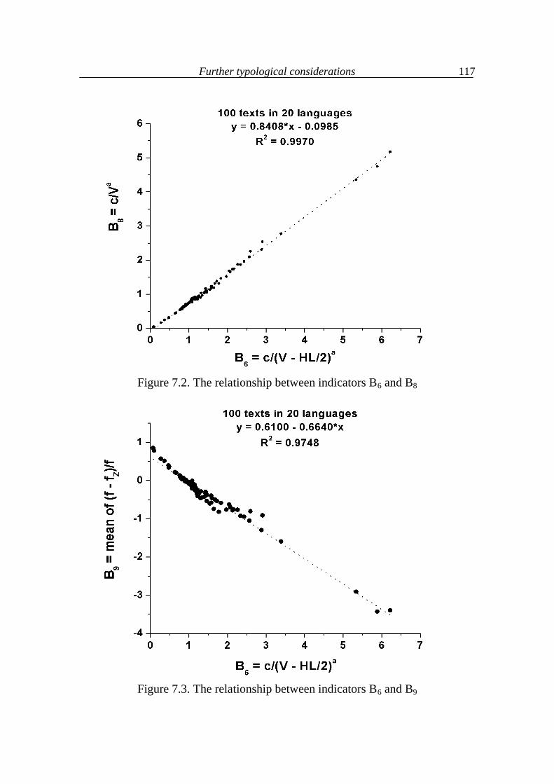
Further typological considerations

117

Figure 7.2. The relationship between indicators B6 and B8

Figure 7.3. The relationship between indicators B6 and B9

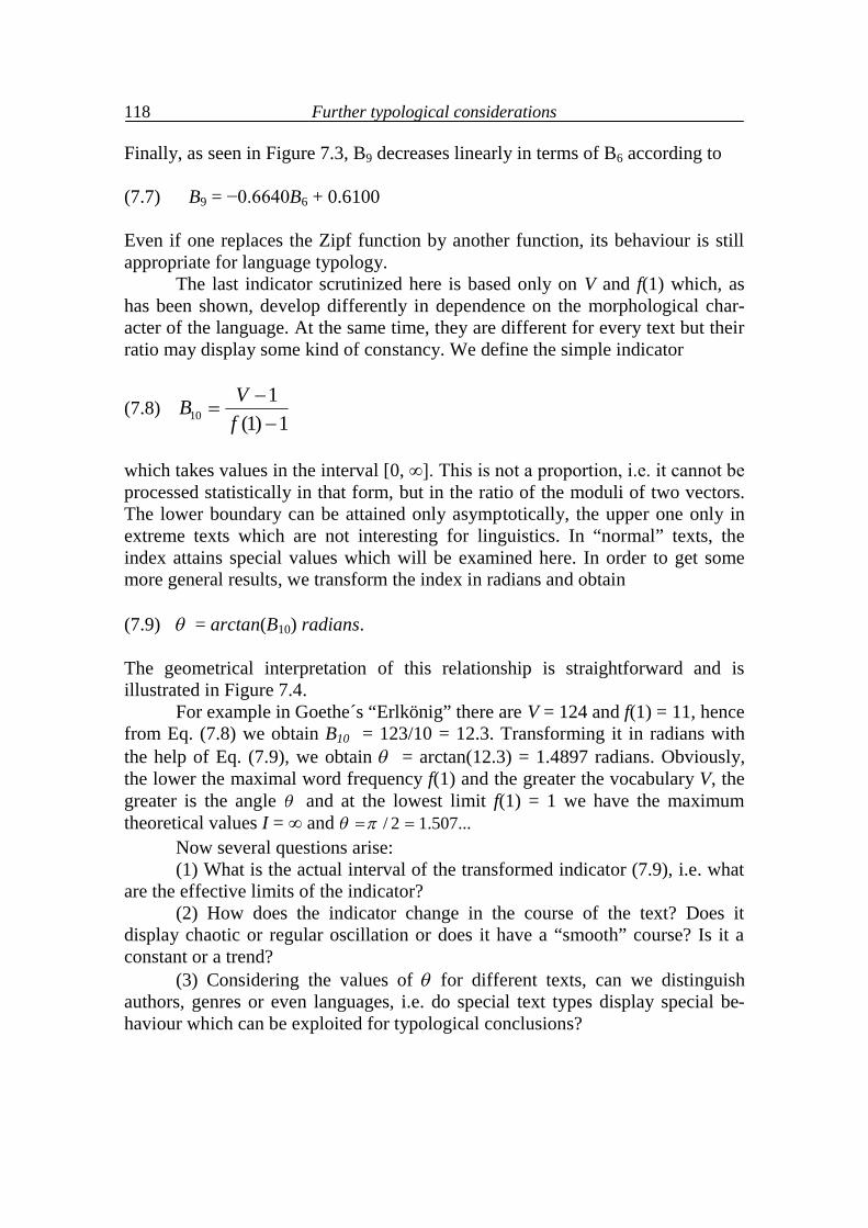
Further typological considerations

118

Finally, as seen in Figure 7.3, B9 decreases linearly in terms of B6 according to (7.7) B9 = −0.6640B6 + 0.6100 Even if one replaces the Zipf function by another function, its behaviour is still appropriate for language typology. The last indicator scrutinized here is based only on V and f(1) which, as has been shown, develop differently in dependence on the morphological char-acter of the language. At the same time, they are different for every text but their ratio may display some kind of constancy. We define the simple indicator

(7.8) 101

(1) 1VBf

which takes values in the interval [0, ∞]. This is not a proportion, i.e. it cannot be processed statistically in that form, but in the ratio of the moduli of two vectors. The lower boundary can be attained only asymptotically, the upper one only in extreme texts which are not interesting for linguistics. In “normal” texts, the index attains special values which will be examined here. In order to get some more general results, we transform the index in radians and obtain (7.9) = arctan(B10) radians. The geometrical interpretation of this relationship is straightforward and is illustrated in Figure 7.4. For example in Goethe´s “Erlkönig” there are V = 124 and f(1) = 11, hence from Eq. (7.8) we obtain B10 = 123/10 = 12.3. Transforming it in radians with the help of Eq. (7.9), we obtain = arctan(12.3) = 1.4897 radians. Obviously, the lower the maximal word frequency f(1) and the greater the vocabulary V, the greater is the angle and at the lowest limit f(1) = 1 we have the maximum theoretical values I = ∞ and / 2 1.507... Now several questions arise: (1) What is the actual interval of the transformed indicator (7.9), i.e. what are the effective limits of the indicator? (2) How does the indicator change in the course of the text? Does it display chaotic or regular oscillation or does it have a “smooth” course? Is it a constant or a trend? (3) Considering the values of for different texts, can we distinguish authors, genres or even languages, i.e. do special text types display special be-haviour which can be exploited for typological conclusions?

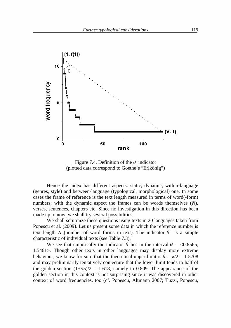
Further typological considerations

119

Figure 7.4. Definition of the indicator

(plotted data correspond to Goethe´s “Erlkönig”) Hence the index has different aspects: static, dynamic, within-language (genres, style) and between-language (typological, morphological) one. In some cases the frame of reference is the text length measured in terms of word(-form) numbers; with the dynamic aspect the frames can be words themselves (N), verses, sentences, chapters etc. Since no investigation in this direction has been made up to now, we shall try several possibilities. We shall scrutinize these questions using texts in 20 languages taken from Popescu et al. (2009). Let us present some data in which the reference number is text length N (number of word forms in text). The indicator is a simple characteristic of individual texts (see Table 7.3). We see that empirically the indicator lies in the interval <0.8565, 1.5461>. Though other texts in other languages may display more extreme behaviour, we know for sure that the theoretical upper limit is = π/2 = 1.5708 and may preliminarily tentatively conjecture that the lower limit tends to half of the golden section (1+5)/2 = 1.618, namely to 0.809. The appearance of the golden section in this context is not surprising since it was discovered in other context of word frequencies, too (cf. Popescu, Altmann 2007; Tuzzi, Popescu,

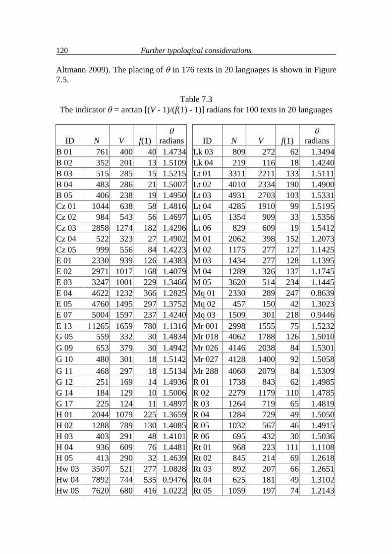
Further typological considerations

120

Altmann 2009). The placing of in 176 texts in 20 languages is shown in Figure 7.5.

Table 7.3 The indicator = arctan [(V - 1)/(f(1) - 1)] radians for 100 texts in 20 languages

ID N V f(1)

radians ID N V f(1)

radians B 01 761 400 40 1.4734 Lk 03 809 272 62 1.3494 B 02 352 201 13 1.5109 Lk 04 219 116 18 1.4240 B 03 515 285 15 1.5215 Lt 01 3311 2211 133 1.5111 B 04 483 286 21 1.5007 Lt 02 4010 2334 190 1.4900 B 05 406 238 19 1.4950 Lt 03 4931 2703 103 1.5331 Cz 01 1044 638 58 1.4816 Lt 04 4285 1910 99 1.5195 Cz 02 984 543 56 1.4697 Lt 05 1354 909 33 1.5356 Cz 03 2858 1274 182 1.4296 Lt 06 829 609 19 1.5412 Cz 04 522 323 27 1.4902 M 01 2062 398 152 1.2073 Cz 05 999 556 84 1.4223 M 02 1175 277 127 1.1425 E 01 2330 939 126 1.4383 M 03 1434 277 128 1.1395 E 02 2971 1017 168 1.4079 M 04 1289 326 137 1.1745 E 03 3247 1001 229 1.3466 M 05 3620 514 234 1.1445 E 04 4622 1232 366 1.2825 Mq 01 2330 289 247 0.8639 E 05 4760 1495 297 1.3752 Mq 02 457 150 42 1.3023 E 07 5004 1597 237 1.4240 Mq 03 1509 301 218 0.9446 E 13 11265 1659 780 1.1316 Mr 001 2998 1555 75 1.5232 G 05 559 332 30 1.4834 Mr 018 4062 1788 126 1.5010 G 09 653 379 30 1.4942 Mr 026 4146 2038 84 1.5301 G 10 480 301 18 1.5142 Mr 027 4128 1400 92 1.5058 G 11 468 297 18 1.5134 Mr 288 4060 2079 84 1.5309 G 12 251 169 14 1.4936 R 01 1738 843 62 1.4985 G 14 184 129 10 1.5006 R 02 2279 1179 110 1.4785 G 17 225 124 11 1.4897 R 03 1264 719 65 1.4819 H 01 2044 1079 225 1.3659 R 04 1284 729 49 1.5050 H 02 1288 789 130 1.4085 R 05 1032 567 46 1.4915 H 03 403 291 48 1.4101 R 06 695 432 30 1.5036 H 04 936 609 76 1.4481 Rt 01 968 223 111 1.1108 H 05 413 290 32 1.4639 Rt 02 845 214 69 1.2618 Hw 03 3507 521 277 1.0828 Rt 03 892 207 66 1.2651 Hw 04 7892 744 535 0.9476 Rt 04 625 181 49 1.3102 Hw 05 7620 680 416 1.0222 Rt 05 1059 197 74 1.2143

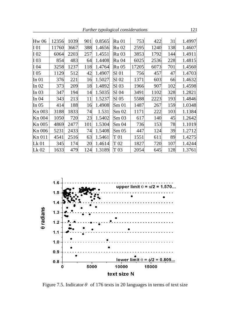
Further typological considerations

121

Hw 06 12356 1039 901 0.8565 Ru 01 753 422 31 1.4997 I 01 11760 3667 388 1.4656 Ru 02 2595 1240 138 1.4607 I 02 6064 2203 257 1.4551 Ru 03 3853 1792 144 1.4911 I 03 854 483 64 1.4408 Ru 04 6025 2536 228 1.4815 I 04 3258 1237 118 1.4764 Ru 05 17205 6073 701 1.4560 I 05 1129 512 42 1.4907 Sl 01 756 457 47 1.4703 In 01 376 221 16 1.5027 Sl 02 1371 603 66 1.4632 In 02 373 209 18 1.4892 Sl 03 1966 907 102 1.4598 In 03 347 194 14 1.5035 Sl 04 3491 1102 328 1.2821 In 04 343 213 11 1.5237 Sl 05 5588 2223 193 1.4846 In 05 414 188 16 1.4908 Sm 01 1487 267 159 1.0348 Kn 003 3188 1833 74 1.531 Sm 02 1171 222 103 1.1384 Kn 004 1050 720 23 1.5402 Sm 03 617 140 45 1.2642 Kn 005 4869 2477 101 1.5304 Sm 04 736 153 78 1.1019 Kn 006 5231 2433 74 1.5408 Sm 05 447 124 39 1.2712 Kn 011 4541 2516 63 1.5461 T 01 1551 611 89 1.4275 Lk 01 345 174 20 1.4614 T 02 1827 720 107 1.4244 Lk 02 1633 479 124 1.3189 T 03 2054 645 128 1.3761

Figure 7.5. Indicator of 176 texts in 20 languages in terms of text size

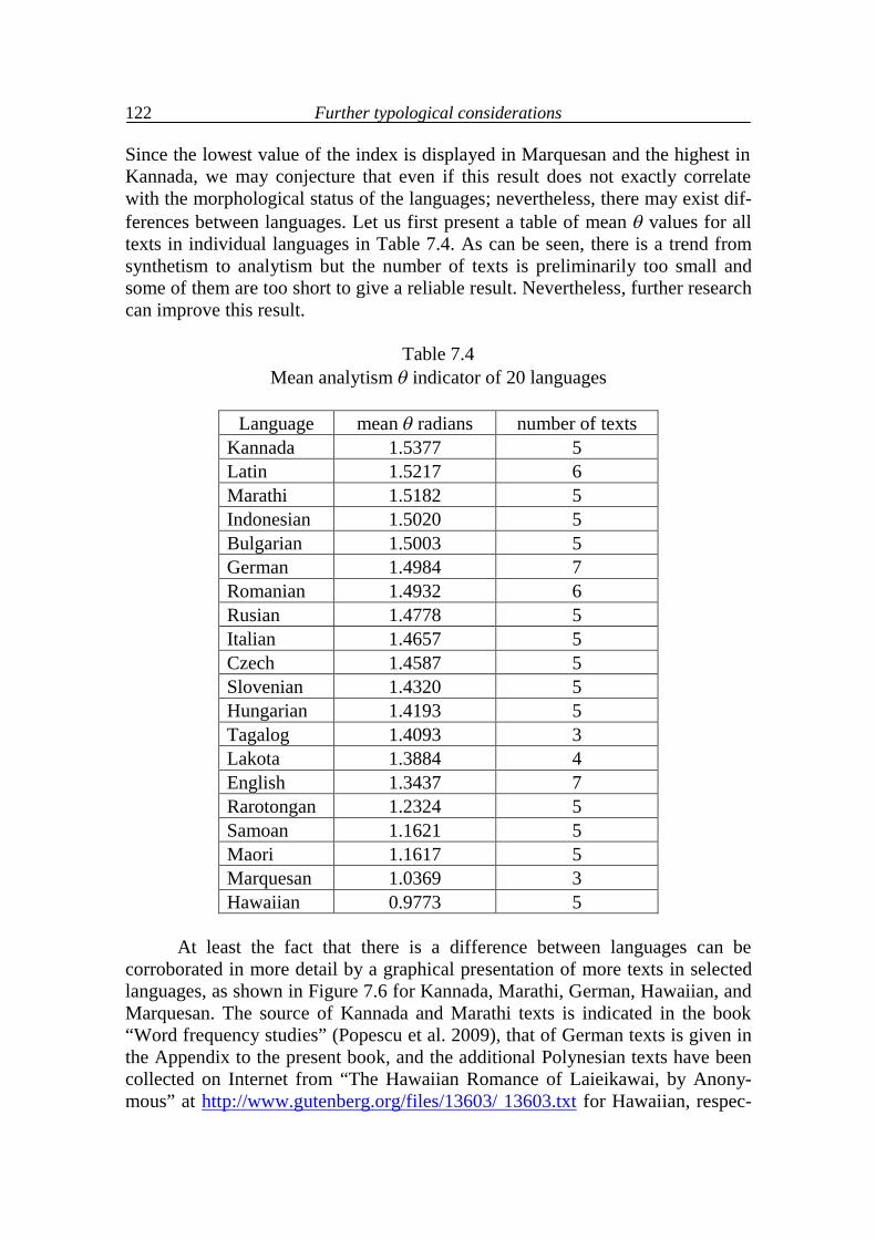
Further typological considerations

122

Since the lowest value of the index is displayed in Marquesan and the highest in Kannada, we may conjecture that even if this result does not exactly correlate with the morphological status of the languages; nevertheless, there may exist dif-ferences between languages. Let us first present a table of mean values for all texts in individual languages in Table 7.4. As can be seen, there is a trend from synthetism to analytism but the number of texts is preliminarily too small and some of them are too short to give a reliable result. Nevertheless, further research can improve this result.

Table 7.4

Mean analytism indicator of 20 languages

Language mean radians number of texts Kannada 1.5377 5 Latin 1.5217 6 Marathi 1.5182 5 Indonesian 1.5020 5 Bulgarian 1.5003 5 German 1.4984 7 Romanian 1.4932 6 Rusian 1.4778 5 Italian 1.4657 5 Czech 1.4587 5 Slovenian 1.4320 5 Hungarian 1.4193 5 Tagalog 1.4093 3 Lakota 1.3884 4 English 1.3437 7 Rarotongan 1.2324 5 Samoan 1.1621 5 Maori 1.1617 5 Marquesan 1.0369 3 Hawaiian 0.9773 5

At least the fact that there is a difference between languages can be

corroborated in more detail by a graphical presentation of more texts in selected languages, as shown in Figure 7.6 for Kannada, Marathi, German, Hawaiian, and Marquesan. The source of Kannada and Marathi texts is indicated in the book “Word frequency studies” (Popescu et al. 2009), that of German texts is given in the Appendix to the present book, and the additional Polynesian texts have been collected on Internet from “The Hawaiian Romance of Laieikawai, by Anony-mous” at http://www.gutenberg.org/files/13603/ 13603.txt for Hawaiian, respec-

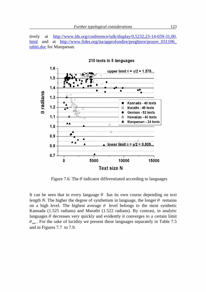
Further typological considerations

123

tively at http://www.lds.org/conference/talk/display/0,5232,23-14-659-31,00. html and at http://www.fides.org/ita/approfondire/preghiere/prayer_031106_ tahiti.doc for Marquesan.

Figure 7.6. The indicator differentiated according to languages

It can be seen that in every language has its own course depending on text length N. The higher the degree of synthetism in language, the longer remains on a high level. The highest average level belongs to the most synthetic Kannada (1.525 radians) and Marathi (1.522 radians). By contrast, in analytic languages decreases very quickly and evidently it converges to a certain limit

min . For the sake of lucidity we present these languages separately in Table 7.5 and in Figures 7.7 to 7.9.

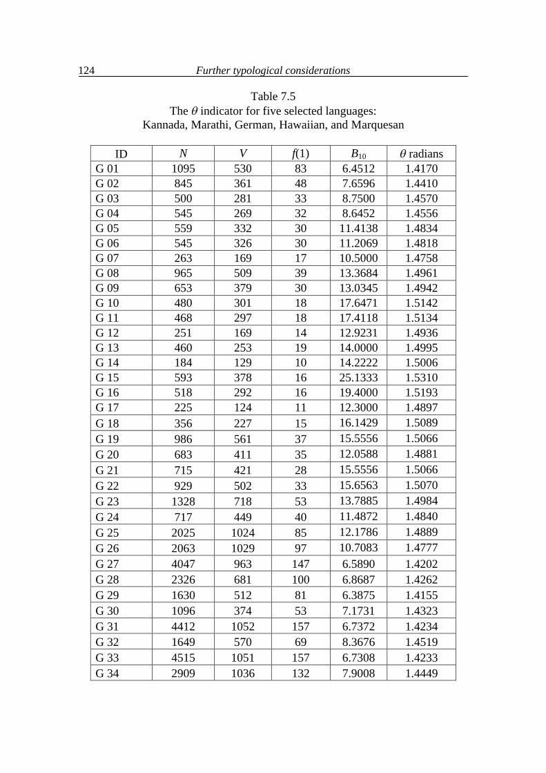
Further typological considerations

124

Table 7.5 The indicator for five selected languages:

Kannada, Marathi, German, Hawaiian, and Marquesan

ID N V f(1) B10 radians G 01 1095 530 83 6.4512 1.4170 G 02 845 361 48 7.6596 1.4410 G 03 500 281 33 8.7500 1.4570 G 04 545 269 32 8.6452 1.4556 G 05 559 332 30 11.4138 1.4834 G 06 545 326 30 11.2069 1.4818 G 07 263 169 17 10.5000 1.4758 G 08 965 509 39 13.3684 1.4961 G 09 653 379 30 13.0345 1.4942 G 10 480 301 18 17.6471 1.5142 G 11 468 297 18 17.4118 1.5134 G 12 251 169 14 12.9231 1.4936 G 13 460 253 19 14.0000 1.4995 G 14 184 129 10 14.2222 1.5006 G 15 593 378 16 25.1333 1.5310 G 16 518 292 16 19.4000 1.5193 G 17 225 124 11 12.3000 1.4897 G 18 356 227 15 16.1429 1.5089 G 19 986 561 37 15.5556 1.5066 G 20 683 411 35 12.0588 1.4881 G 21 715 421 28 15.5556 1.5066 G 22 929 502 33 15.6563 1.5070 G 23 1328 718 53 13.7885 1.4984 G 24 717 449 40 11.4872 1.4840 G 25 2025 1024 85 12.1786 1.4889 G 26 2063 1029 97 10.7083 1.4777 G 27 4047 963 147 6.5890 1.4202 G 28 2326 681 100 6.8687 1.4262 G 29 1630 512 81 6.3875 1.4155 G 30 1096 374 53 7.1731 1.4323 G 31 4412 1052 157 6.7372 1.4234 G 32 1649 570 69 8.3676 1.4519 G 33 4515 1051 157 6.7308 1.4233 G 34 2909 1036 132 7.9008 1.4449

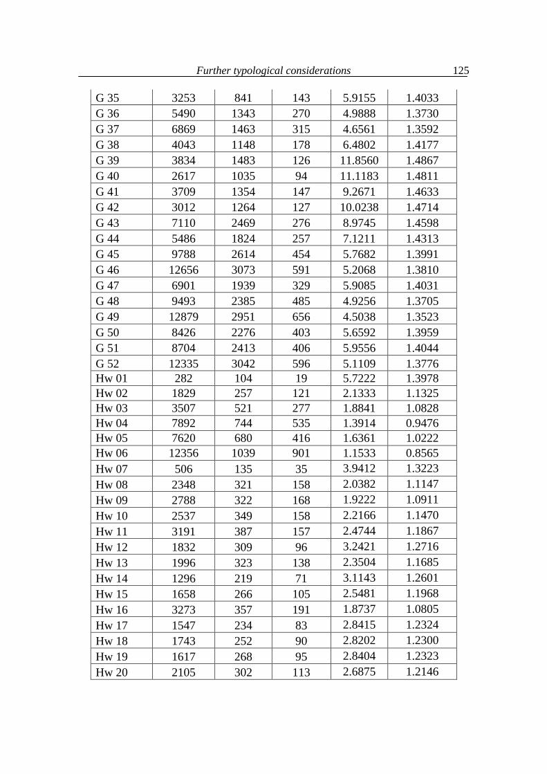
Further typological considerations

125

G 35 3253 841 143 5.9155 1.4033 G 36 5490 1343 270 4.9888 1.3730 G 37 6869 1463 315 4.6561 1.3592 G 38 4043 1148 178 6.4802 1.4177 G 39 3834 1483 126 11.8560 1.4867 G 40 2617 1035 94 11.1183 1.4811 G 41 3709 1354 147 9.2671 1.4633 G 42 3012 1264 127 10.0238 1.4714 G 43 7110 2469 276 8.9745 1.4598 G 44 5486 1824 257 7.1211 1.4313 G 45 9788 2614 454 5.7682 1.3991 G 46 12656 3073 591 5.2068 1.3810 G 47 6901 1939 329 5.9085 1.4031 G 48 9493 2385 485 4.9256 1.3705 G 49 12879 2951 656 4.5038 1.3523 G 50 8426 2276 403 5.6592 1.3959 G 51 8704 2413 406 5.9556 1.4044 G 52 12335 3042 596 5.1109 1.3776 Hw 01 282 104 19 5.7222 1.3978 Hw 02 1829 257 121 2.1333 1.1325 Hw 03 3507 521 277 1.8841 1.0828 Hw 04 7892 744 535 1.3914 0.9476 Hw 05 7620 680 416 1.6361 1.0222 Hw 06 12356 1039 901 1.1533 0.8565 Hw 07 506 135 35 3.9412 1.3223 Hw 08 2348 321 158 2.0382 1.1147 Hw 09 2788 322 168 1.9222 1.0911 Hw 10 2537 349 158 2.2166 1.1470 Hw 11 3191 387 157 2.4744 1.1867 Hw 12 1832 309 96 3.2421 1.2716 Hw 13 1996 323 138 2.3504 1.1685 Hw 14 1296 219 71 3.1143 1.2601 Hw 15 1658 266 105 2.5481 1.1968 Hw 16 3273 357 191 1.8737 1.0805 Hw 17 1547 234 83 2.8415 1.2324 Hw 18 1743 252 90 2.8202 1.2300 Hw 19 1617 268 95 2.8404 1.2323 Hw 20 2105 302 113 2.6875 1.2146

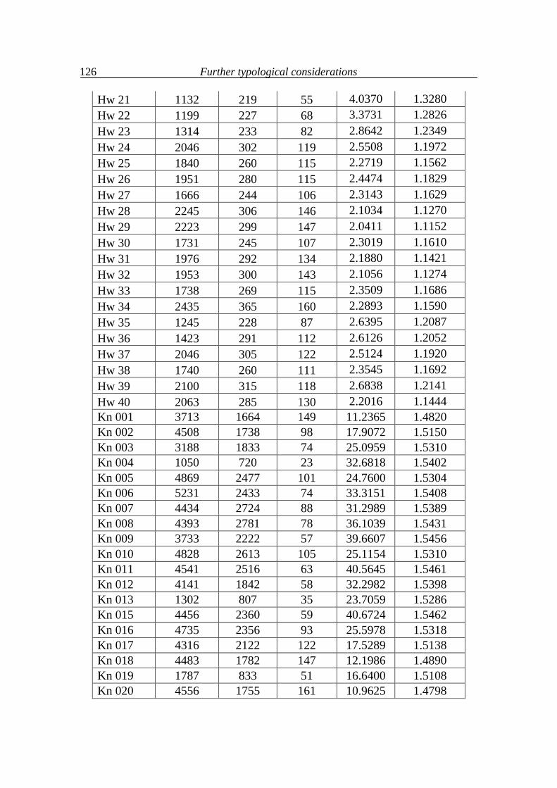
Further typological considerations

126

Hw 21 1132 219 55 4.0370 1.3280 Hw 22 1199 227 68 3.3731 1.2826 Hw 23 1314 233 82 2.8642 1.2349 Hw 24 2046 302 119 2.5508 1.1972 Hw 25 1840 260 115 2.2719 1.1562 Hw 26 1951 280 115 2.4474 1.1829 Hw 27 1666 244 106 2.3143 1.1629 Hw 28 2245 306 146 2.1034 1.1270 Hw 29 2223 299 147 2.0411 1.1152 Hw 30 1731 245 107 2.3019 1.1610 Hw 31 1976 292 134 2.1880 1.1421 Hw 32 1953 300 143 2.1056 1.1274 Hw 33 1738 269 115 2.3509 1.1686 Hw 34 2435 365 160 2.2893 1.1590 Hw 35 1245 228 87 2.6395 1.2087 Hw 36 1423 291 112 2.6126 1.2052 Hw 37 2046 305 122 2.5124 1.1920 Hw 38 1740 260 111 2.3545 1.1692 Hw 39 2100 315 118 2.6838 1.2141 Hw 40 2063 285 130 2.2016 1.1444 Kn 001 3713 1664 149 11.2365 1.4820 Kn 002 4508 1738 98 17.9072 1.5150 Kn 003 3188 1833 74 25.0959 1.5310 Kn 004 1050 720 23 32.6818 1.5402 Kn 005 4869 2477 101 24.7600 1.5304 Kn 006 5231 2433 74 33.3151 1.5408 Kn 007 4434 2724 88 31.2989 1.5389 Kn 008 4393 2781 78 36.1039 1.5431 Kn 009 3733 2222 57 39.6607 1.5456 Kn 010 4828 2613 105 25.1154 1.5310 Kn 011 4541 2516 63 40.5645 1.5461 Kn 012 4141 1842 58 32.2982 1.5398 Kn 013 1302 807 35 23.7059 1.5286 Kn 015 4456 2360 59 40.6724 1.5462 Kn 016 4735 2356 93 25.5978 1.5318 Kn 017 4316 2122 122 17.5289 1.5138 Kn 018 4483 1782 147 12.1986 1.4890 Kn 019 1787 833 51 16.6400 1.5108 Kn 020 4556 1755 161 10.9625 1.4798

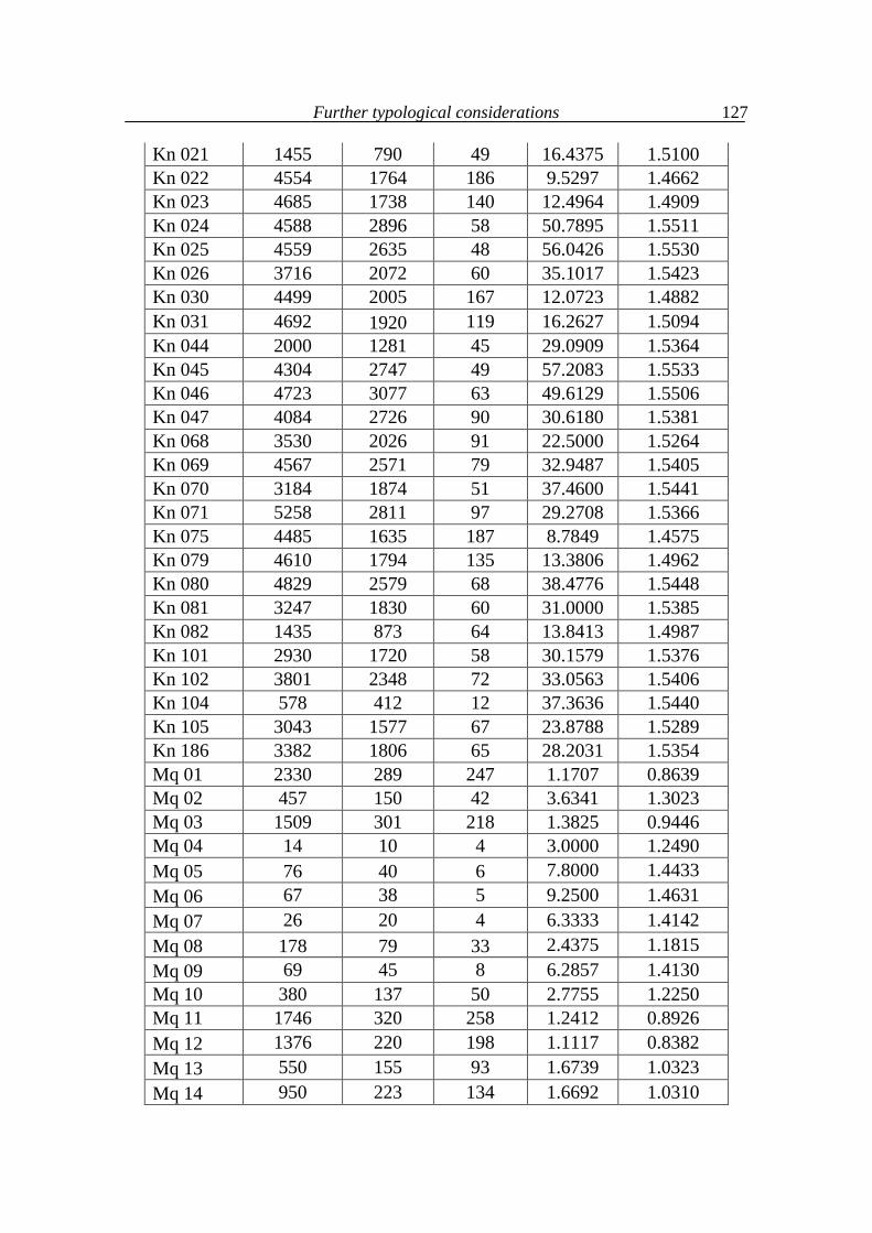
Further typological considerations

127

Kn 021 1455 790 49 16.4375 1.5100 Kn 022 4554 1764 186 9.5297 1.4662 Kn 023 4685 1738 140 12.4964 1.4909 Kn 024 4588 2896 58 50.7895 1.5511 Kn 025 4559 2635 48 56.0426 1.5530 Kn 026 3716 2072 60 35.1017 1.5423 Kn 030 4499 2005 167 12.0723 1.4882 Kn 031 4692 1920 119 16.2627 1.5094 Kn 044 2000 1281 45 29.0909 1.5364 Kn 045 4304 2747 49 57.2083 1.5533 Kn 046 4723 3077 63 49.6129 1.5506 Kn 047 4084 2726 90 30.6180 1.5381 Kn 068 3530 2026 91 22.5000 1.5264 Kn 069 4567 2571 79 32.9487 1.5405 Kn 070 3184 1874 51 37.4600 1.5441 Kn 071 5258 2811 97 29.2708 1.5366 Kn 075 4485 1635 187 8.7849 1.4575 Kn 079 4610 1794 135 13.3806 1.4962 Kn 080 4829 2579 68 38.4776 1.5448 Kn 081 3247 1830 60 31.0000 1.5385 Kn 082 1435 873 64 13.8413 1.4987 Kn 101 2930 1720 58 30.1579 1.5376 Kn 102 3801 2348 72 33.0563 1.5406 Kn 104 578 412 12 37.3636 1.5440 Kn 105 3043 1577 67 23.8788 1.5289 Kn 186 3382 1806 65 28.2031 1.5354 Mq 01 2330 289 247 1.1707 0.8639 Mq 02 457 150 42 3.6341 1.3023 Mq 03 1509 301 218 1.3825 0.9446 Mq 04 14 10 4 3.0000 1.2490 Mq 05 76 40 6 7.8000 1.4433 Mq 06 67 38 5 9.2500 1.4631 Mq 07 26 20 4 6.3333 1.4142 Mq 08 178 79 33 2.4375 1.1815 Mq 09 69 45 8 6.2857 1.4130 Mq 10 380 137 50 2.7755 1.2250 Mq 11 1746 320 258 1.2412 0.8926 Mq 12 1376 220 198 1.1117 0.8382 Mq 13 550 155 93 1.6739 1.0323 Mq 14 950 223 134 1.6692 1.0310

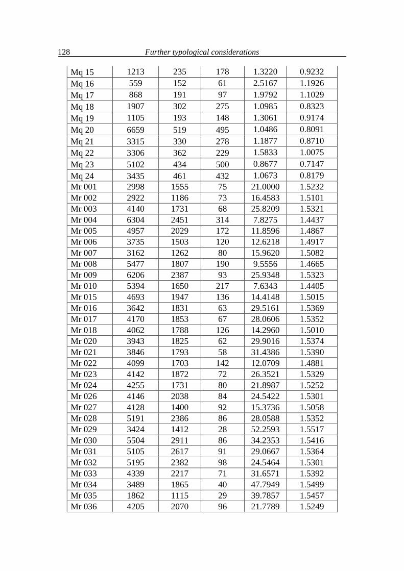
Further typological considerations

128

Mq 15 1213 235 178 1.3220 0.9232 Mq 16 559 152 61 2.5167 1.1926 Mq 17 868 191 97 1.9792 1.1029 Mq 18 1907 302 275 1.0985 0.8323 Mq 19 1105 193 148 1.3061 0.9174 Mq 20 6659 519 495 1.0486 0.8091 Mq 21 3315 330 278 1.1877 0.8710 Mq 22 3306 362 229 1.5833 1.0075 Mq 23 5102 434 500 0.8677 0.7147 Mq 24 3435 461 432 1.0673 0.8179 Mr 001 2998 1555 75 21.0000 1.5232 Mr 002 2922 1186 73 16.4583 1.5101 Mr 003 4140 1731 68 25.8209 1.5321 Mr 004 6304 2451 314 7.8275 1.4437 Mr 005 4957 2029 172 11.8596 1.4867 Mr 006 3735 1503 120 12.6218 1.4917 Mr 007 3162 1262 80 15.9620 1.5082 Mr 008 5477 1807 190 9.5556 1.4665 Mr 009 6206 2387 93 25.9348 1.5323 Mr 010 5394 1650 217 7.6343 1.4405 Mr 015 4693 1947 136 14.4148 1.5015 Mr 016 3642 1831 63 29.5161 1.5369 Mr 017 4170 1853 67 28.0606 1.5352 Mr 018 4062 1788 126 14.2960 1.5010 Mr 020 3943 1825 62 29.9016 1.5374 Mr 021 3846 1793 58 31.4386 1.5390 Mr 022 4099 1703 142 12.0709 1.4881 Mr 023 4142 1872 72 26.3521 1.5329 Mr 024 4255 1731 80 21.8987 1.5252 Mr 026 4146 2038 84 24.5422 1.5301 Mr 027 4128 1400 92 15.3736 1.5058 Mr 028 5191 2386 86 28.0588 1.5352 Mr 029 3424 1412 28 52.2593 1.5517 Mr 030 5504 2911 86 34.2353 1.5416 Mr 031 5105 2617 91 29.0667 1.5364 Mr 032 5195 2382 98 24.5464 1.5301 Mr 033 4339 2217 71 31.6571 1.5392 Mr 034 3489 1865 40 47.7949 1.5499 Mr 035 1862 1115 29 39.7857 1.5457 Mr 036 4205 2070 96 21.7789 1.5249

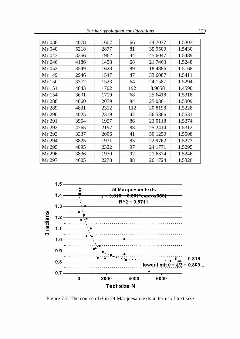
Further typological considerations

129

Mr 038 4078 1607 66 24.7077 1.5303 Mr 040 5218 2877 81 35.9500 1.5430 Mr 043 3356 1962 44 45.6047 1.5489 Mr 046 4186 1458 68 21.7463 1.5248 Mr 052 3549 1628 89 18.4886 1.5168 Mr 149 2946 1547 47 33.6087 1.5411 Mr 150 3372 1523 64 24.1587 1.5294 Mr 151 4843 1702 192 8.9058 1.4590 Mr 154 3601 1719 68 25.6418 1.5318 Mr 288 4060 2079 84 25.0361 1.5309 Mr 289 4831 2312 112 20.8198 1.5228 Mr 290 4025 2319 42 56.5366 1.5531 Mr 291 3954 1957 86 23.0118 1.5274 Mr 292 4765 2197 88 25.2414 1.5312 Mr 293 3337 2006 41 50.1250 1.5508 Mr 294 3825 1931 85 22.9762 1.5273 Mr 295 4895 2322 97 24.1771 1.5295 Mr 296 3836 1970 92 21.6374 1.5246 Mr 297 4605 2278 88 26.1724 1.5326

Figure 7.7. The course of in 24 Marquesan texts in terms of text size

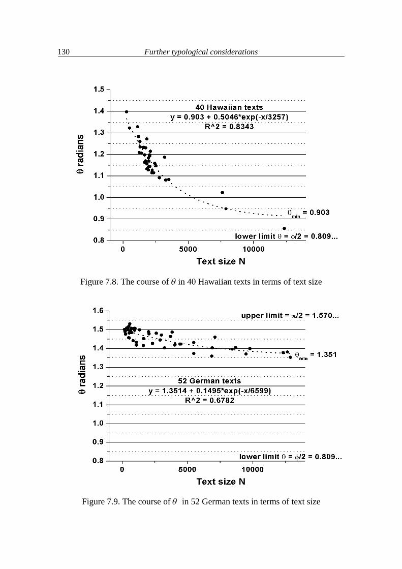
Further typological considerations

130

Figure 7.8. The course of in 40 Hawaiian texts in terms of text size

Figure 7.9. The course of in 52 German texts in terms of text size

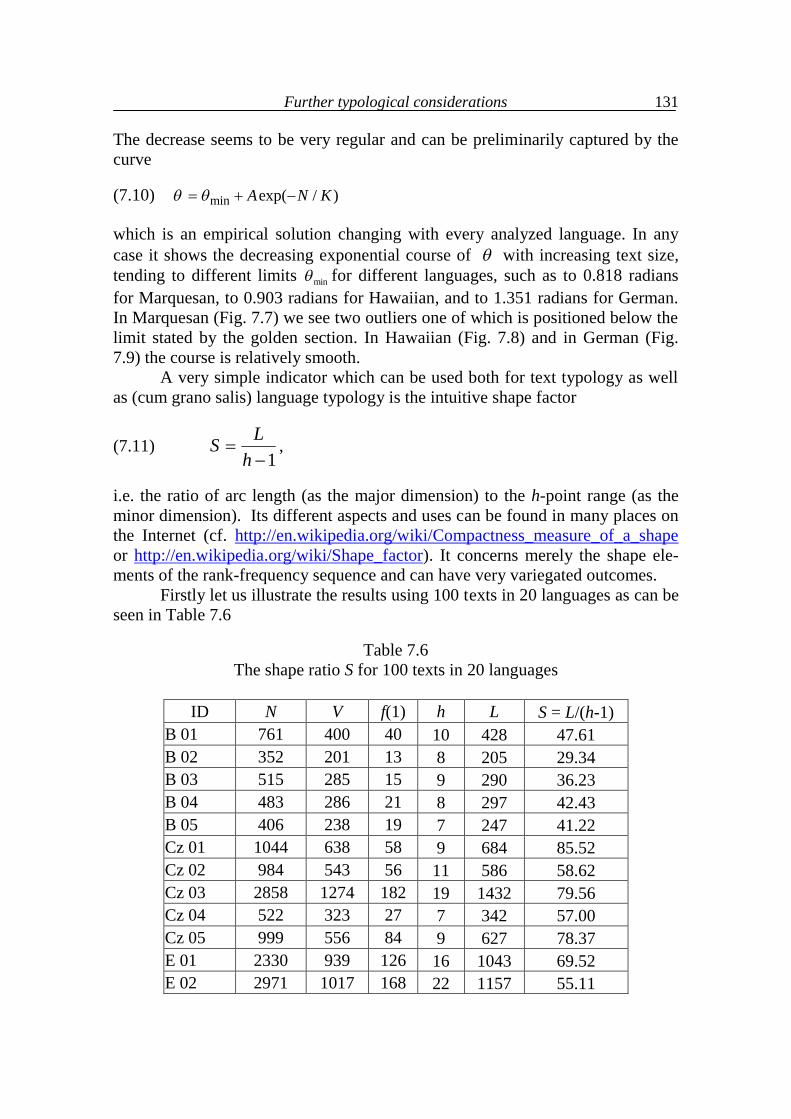
Further typological considerations

131

The decrease seems to be very regular and can be preliminarily captured by the curve (7.10) min exp( / )A N K which is an empirical solution changing with every analyzed language. In any case it shows the decreasing exponential course of with increasing text size, tending to different limits min for different languages, such as to 0.818 radians for Marquesan, to 0.903 radians for Hawaiian, and to 1.351 radians for German. In Marquesan (Fig. 7.7) we see two outliers one of which is positioned below the limit stated by the golden section. In Hawaiian (Fig. 7.8) and in German (Fig. 7.9) the course is relatively smooth. A very simple indicator which can be used both for text typology as well as (cum grano salis) language typology is the intuitive shape factor

(7.11) 1

LSh

,

i.e. the ratio of arc length (as the major dimension) to the h-point range (as the minor dimension). Its different aspects and uses can be found in many places on the Internet (cf. http://en.wikipedia.org/wiki/Compactness_measure_of_a_shape or http://en.wikipedia.org/wiki/Shape_factor). It concerns merely the shape ele-ments of the rank-frequency sequence and can have very variegated outcomes. Firstly let us illustrate the results using 100 texts in 20 languages as can be seen in Table 7.6

Table 7.6 The shape ratio S for 100 texts in 20 languages

ID N V f(1) h L S = L/(h-1)

B 01 761 400 40 10 428 47.61 B 02 352 201 13 8 205 29.34 B 03 515 285 15 9 290 36.23 B 04 483 286 21 8 297 42.43 B 05 406 238 19 7 247 41.22 Cz 01 1044 638 58 9 684 85.52 Cz 02 984 543 56 11 586 58.62 Cz 03 2858 1274 182 19 1432 79.56 Cz 04 522 323 27 7 342 57.00 Cz 05 999 556 84 9 627 78.37 E 01 2330 939 126 16 1043 69.52 E 02 2971 1017 168 22 1157 55.11

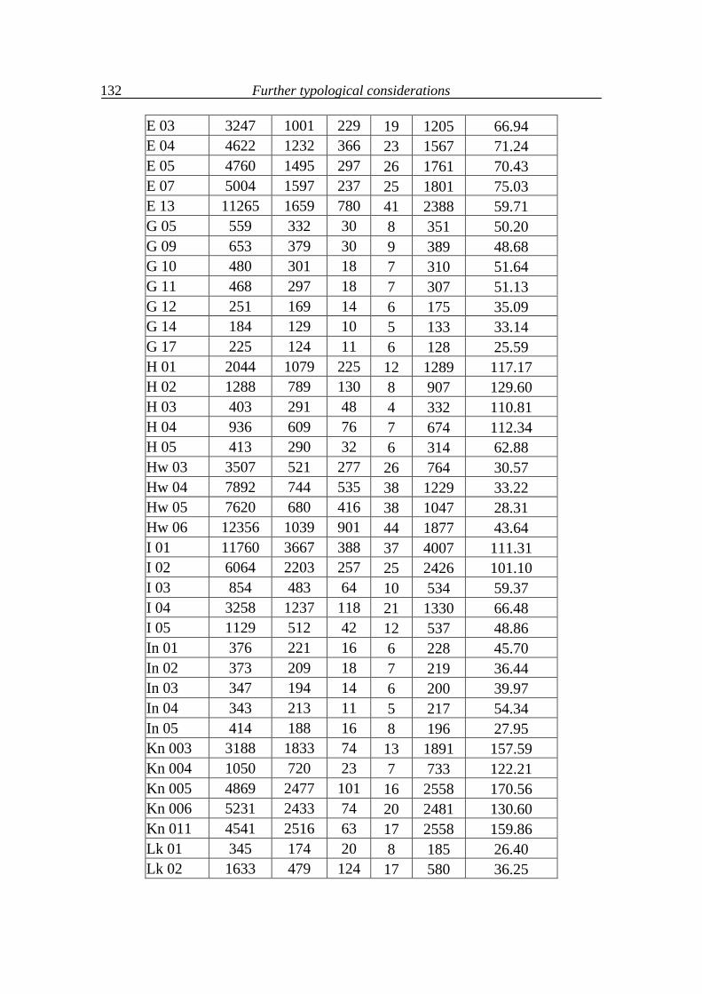
Further typological considerations

132

E 03 3247 1001 229 19 1205 66.94 E 04 4622 1232 366 23 1567 71.24 E 05 4760 1495 297 26 1761 70.43 E 07 5004 1597 237 25 1801 75.03 E 13 11265 1659 780 41 2388 59.71 G 05 559 332 30 8 351 50.20 G 09 653 379 30 9 389 48.68 G 10 480 301 18 7 310 51.64 G 11 468 297 18 7 307 51.13 G 12 251 169 14 6 175 35.09 G 14 184 129 10 5 133 33.14 G 17 225 124 11 6 128 25.59 H 01 2044 1079 225 12 1289 117.17 H 02 1288 789 130 8 907 129.60 H 03 403 291 48 4 332 110.81 H 04 936 609 76 7 674 112.34 H 05 413 290 32 6 314 62.88 Hw 03 3507 521 277 26 764 30.57 Hw 04 7892 744 535 38 1229 33.22 Hw 05 7620 680 416 38 1047 28.31 Hw 06 12356 1039 901 44 1877 43.64 I 01 11760 3667 388 37 4007 111.31 I 02 6064 2203 257 25 2426 101.10 I 03 854 483 64 10 534 59.37 I 04 3258 1237 118 21 1330 66.48 I 05 1129 512 42 12 537 48.86 In 01 376 221 16 6 228 45.70 In 02 373 209 18 7 219 36.44 In 03 347 194 14 6 200 39.97 In 04 343 213 11 5 217 54.34 In 05 414 188 16 8 196 27.95 Kn 003 3188 1833 74 13 1891 157.59 Kn 004 1050 720 23 7 733 122.21 Kn 005 4869 2477 101 16 2558 170.56 Kn 006 5231 2433 74 20 2481 130.60 Kn 011 4541 2516 63 17 2558 159.86 Lk 01 345 174 20 8 185 26.40 Lk 02 1633 479 124 17 580 36.25

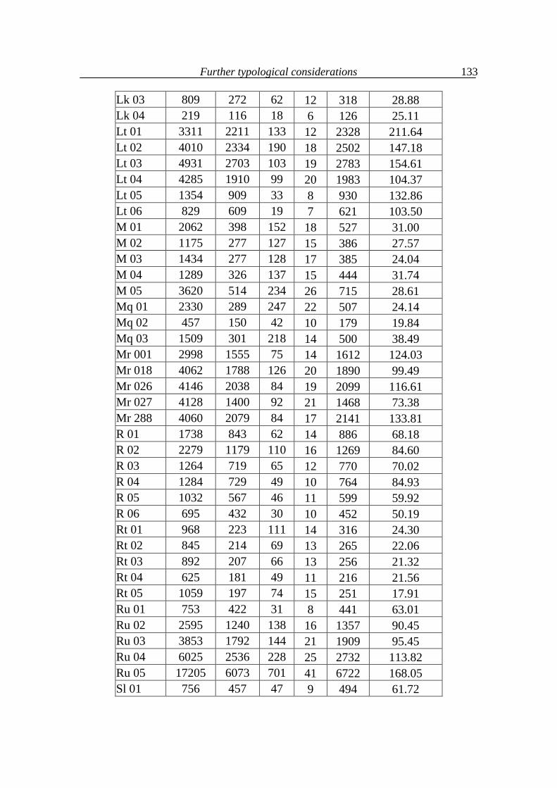
Further typological considerations

133

Lk 03 809 272 62 12 318 28.88 Lk 04 219 116 18 6 126 25.11 Lt 01 3311 2211 133 12 2328 211.64 Lt 02 4010 2334 190 18 2502 147.18 Lt 03 4931 2703 103 19 2783 154.61 Lt 04 4285 1910 99 20 1983 104.37 Lt 05 1354 909 33 8 930 132.86 Lt 06 829 609 19 7 621 103.50 M 01 2062 398 152 18 527 31.00 M 02 1175 277 127 15 386 27.57 M 03 1434 277 128 17 385 24.04 M 04 1289 326 137 15 444 31.74 M 05 3620 514 234 26 715 28.61 Mq 01 2330 289 247 22 507 24.14 Mq 02 457 150 42 10 179 19.84 Mq 03 1509 301 218 14 500 38.49 Mr 001 2998 1555 75 14 1612 124.03 Mr 018 4062 1788 126 20 1890 99.49 Mr 026 4146 2038 84 19 2099 116.61 Mr 027 4128 1400 92 21 1468 73.38 Mr 288 4060 2079 84 17 2141 133.81 R 01 1738 843 62 14 886 68.18 R 02 2279 1179 110 16 1269 84.60 R 03 1264 719 65 12 770 70.02 R 04 1284 729 49 10 764 84.93 R 05 1032 567 46 11 599 59.92 R 06 695 432 30 10 452 50.19 Rt 01 968 223 111 14 316 24.30 Rt 02 845 214 69 13 265 22.06 Rt 03 892 207 66 13 256 21.32 Rt 04 625 181 49 11 216 21.56 Rt 05 1059 197 74 15 251 17.91 Ru 01 753 422 31 8 441 63.01 Ru 02 2595 1240 138 16 1357 90.45 Ru 03 3853 1792 144 21 1909 95.45 Ru 04 6025 2536 228 25 2732 113.82 Ru 05 17205 6073 701 41 6722 168.05 Sl 01 756 457 47 9 494 61.72

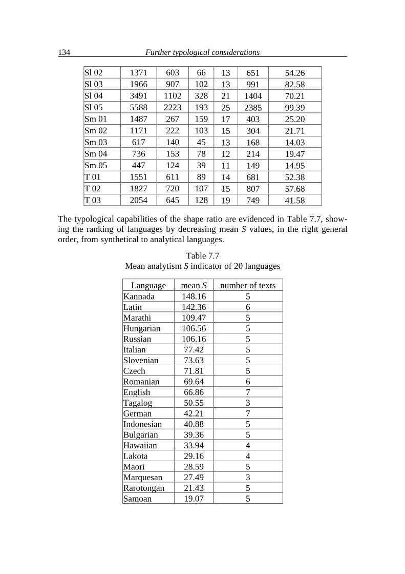
Further typological considerations

134

Sl 02 1371 603 66 13 651 54.26 Sl 03 1966 907 102 13 991 82.58 Sl 04 3491 1102 328 21 1404 70.21 Sl 05 5588 2223 193 25 2385 99.39 Sm 01 1487 267 159 17 403 25.20 Sm 02 1171 222 103 15 304 21.71 Sm 03 617 140 45 13 168 14.03 Sm 04 736 153 78 12 214 19.47 Sm 05 447 124 39 11 149 14.95 T 01 1551 611 89 14 681 52.38 T 02 1827 720 107 15 807 57.68 T 03 2054 645 128 19 749 41.58

The typological capabilities of the shape ratio are evidenced in Table 7.7, show-ing the ranking of languages by decreasing mean S values, in the right general order, from synthetical to analytical languages.

Table 7.7 Mean analytism S indicator of 20 languages

Language mean S number of texts

Kannada 148.16 5 Latin 142.36 6 Marathi 109.47 5 Hungarian 106.56 5 Russian 106.16 5 Italian 77.42 5 Slovenian 73.63 5 Czech 71.81 5 Romanian 69.64 6 English 66.86 7 Tagalog 50.55 3 German 42.21 7 Indonesian 40.88 5 Bulgarian 39.36 5 Hawaiian 33.94 4 Lakota 29.16 4 Maori 28.59 5 Marquesan 27.49 3 Rarotongan 21.43 5 Samoan 19.07 5

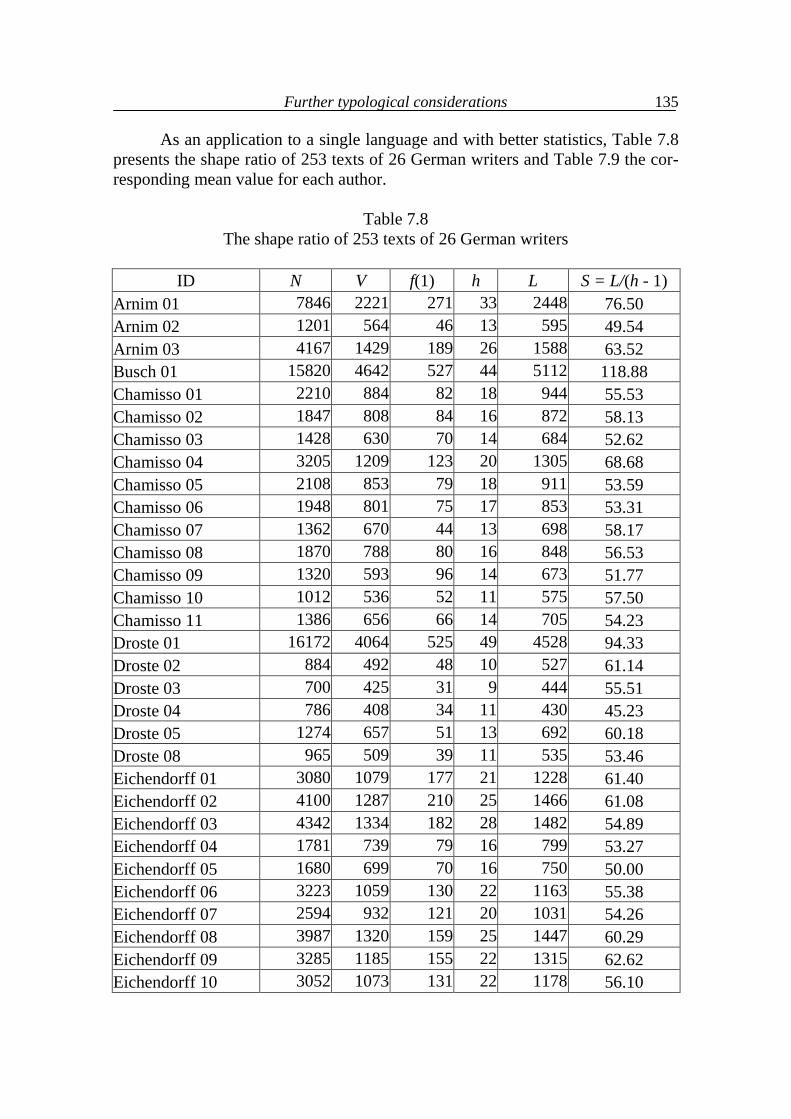
Further typological considerations

135

As an application to a single language and with better statistics, Table 7.8 presents the shape ratio of 253 texts of 26 German writers and Table 7.9 the cor-responding mean value for each author.

Table 7.8 The shape ratio of 253 texts of 26 German writers

ID N V f(1) h L S = L/(h - 1)

Arnim 01 7846 2221 271 33 2448 76.50 Arnim 02 1201 564 46 13 595 49.54 Arnim 03 4167 1429 189 26 1588 63.52 Busch 01 15820 4642 527 44 5112 118.88 Chamisso 01 2210 884 82 18 944 55.53 Chamisso 02 1847 808 84 16 872 58.13 Chamisso 03 1428 630 70 14 684 52.62 Chamisso 04 3205 1209 123 20 1305 68.68 Chamisso 05 2108 853 79 18 911 53.59 Chamisso 06 1948 801 75 17 853 53.31 Chamisso 07 1362 670 44 13 698 58.17 Chamisso 08 1870 788 80 16 848 56.53 Chamisso 09 1320 593 96 14 673 51.77 Chamisso 10 1012 536 52 11 575 57.50 Chamisso 11 1386 656 66 14 705 54.23 Droste 01 16172 4064 525 49 4528 94.33 Droste 02 884 492 48 10 527 61.14 Droste 03 700 425 31 9 444 55.51 Droste 04 786 408 34 11 430 45.23 Droste 05 1274 657 51 13 692 60.18 Droste 08 965 509 39 11 535 53.46 Eichendorff 01 3080 1079 177 21 1228 61.40 Eichendorff 02 4100 1287 210 25 1466 61.08 Eichendorff 03 4342 1334 182 28 1482 54.89 Eichendorff 04 1781 739 79 16 799 53.27 Eichendorff 05 1680 699 70 16 750 50.00 Eichendorff 06 3223 1059 130 22 1163 55.38 Eichendorff 07 2594 932 121 20 1031 54.26 Eichendorff 08 3987 1320 159 25 1447 60.29 Eichendorff 09 3285 1185 155 22 1315 62.62 Eichendorff 10 3052 1073 131 22 1178 56.10

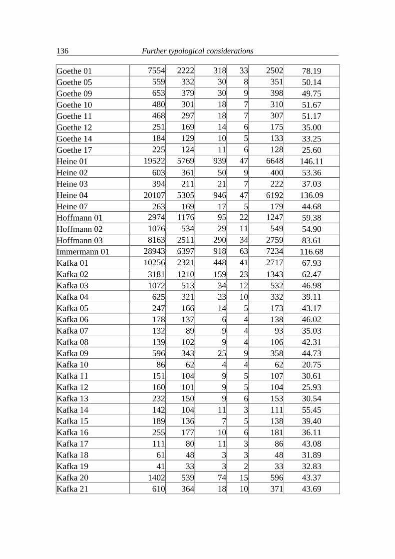
Further typological considerations

136

Goethe 01 7554 2222 318 33 2502 78.19 Goethe 05 559 332 30 8 351 50.14 Goethe 09 653 379 30 9 398 49.75 Goethe 10 480 301 18 7 310 51.67 Goethe 11 468 297 18 7 307 51.17 Goethe 12 251 169 14 6 175 35.00 Goethe 14 184 129 10 5 133 33.25 Goethe 17 225 124 11 6 128 25.60 Heine 01 19522 5769 939 47 6648 146.11 Heine 02 603 361 50 9 400 53.36 Heine 03 394 211 21 7 222 37.03 Heine 04 20107 5305 946 47 6192 136.09 Heine 07 263 169 17 5 179 44.68 Hoffmann 01 2974 1176 95 22 1247 59.38 Hoffmann 02 1076 534 29 11 549 54.90 Hoffmann 03 8163 2511 290 34 2759 83.61 Immermann 01 28943 6397 918 63 7234 116.68 Kafka 01 10256 2321 448 41 2717 67.93 Kafka 02 3181 1210 159 23 1343 62.47 Kafka 03 1072 513 34 12 532 46.98 Kafka 04 625 321 23 10 332 39.11 Kafka 05 247 166 14 5 173 43.17 Kafka 06 178 137 6 4 138 46.02 Kafka 07 132 89 9 4 93 35.03 Kafka 08 139 102 9 4 106 42.31 Kafka 09 596 343 25 9 358 44.73 Kafka 10 86 62 4 4 62 20.75 Kafka 11 151 104 9 5 107 30.61 Kafka 12 160 101 9 5 104 25.93 Kafka 13 232 150 9 6 153 30.54 Kafka 14 142 104 11 3 111 55.45 Kafka 15 189 136 7 5 138 39.40 Kafka 16 255 177 10 6 181 36.11 Kafka 17 111 80 11 3 86 43.08 Kafka 18 61 48 3 3 48 31.89 Kafka 19 41 33 3 2 33 32.83 Kafka 20 1402 539 74 15 596 43.37 Kafka 21 610 364 18 10 371 43.69

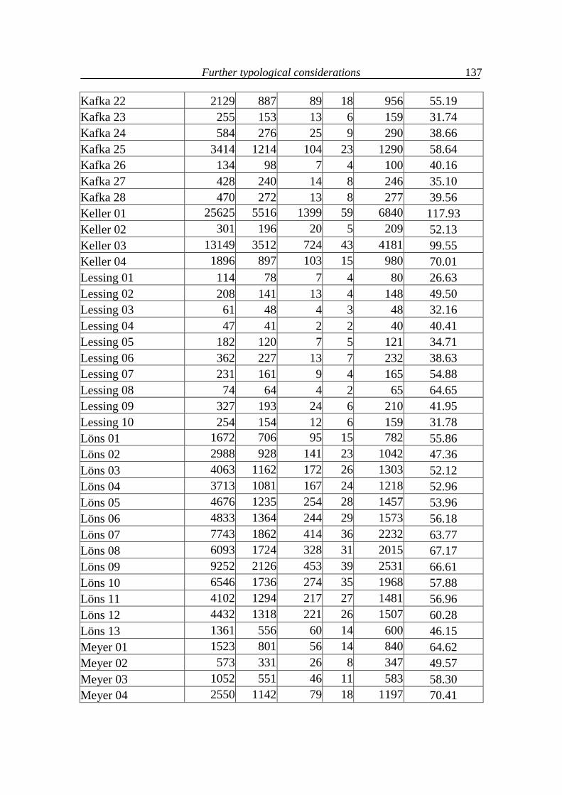
Further typological considerations

137

Kafka 22 2129 887 89 18 956 55.19 Kafka 23 255 153 13 6 159 31.74 Kafka 24 584 276 25 9 290 38.66 Kafka 25 3414 1214 104 23 1290 58.64 Kafka 26 134 98 7 4 100 40.16 Kafka 27 428 240 14 8 246 35.10 Kafka 28 470 272 13 8 277 39.56 Keller 01 25625 5516 1399 59 6840 117.93 Keller 02 301 196 20 5 209 52.13 Keller 03 13149 3512 724 43 4181 99.55 Keller 04 1896 897 103 15 980 70.01 Lessing 01 114 78 7 4 80 26.63 Lessing 02 208 141 13 4 148 49.50 Lessing 03 61 48 4 3 48 32.16 Lessing 04 47 41 2 2 40 40.41 Lessing 05 182 120 7 5 121 34.71 Lessing 06 362 227 13 7 232 38.63 Lessing 07 231 161 9 4 165 54.88 Lessing 08 74 64 4 2 65 64.65 Lessing 09 327 193 24 6 210 41.95 Lessing 10 254 154 12 6 159 31.78 Löns 01 1672 706 95 15 782 55.86 Löns 02 2988 928 141 23 1042 47.36 Löns 03 4063 1162 172 26 1303 52.12 Löns 04 3713 1081 167 24 1218 52.96 Löns 05 4676 1235 254 28 1457 53.96 Löns 06 4833 1364 244 29 1573 56.18 Löns 07 7743 1862 414 36 2232 63.77 Löns 08 6093 1724 328 31 2015 67.17 Löns 09 9252 2126 453 39 2531 66.61 Löns 10 6546 1736 274 35 1968 57.88 Löns 11 4102 1294 217 27 1481 56.96 Löns 12 4432 1318 221 26 1507 60.28 Löns 13 1361 556 60 14 600 46.15 Meyer 01 1523 801 56 14 840 64.62 Meyer 02 573 331 26 8 347 49.57 Meyer 03 1052 551 46 11 583 58.30 Meyer 04 2550 1142 79 18 1197 70.41

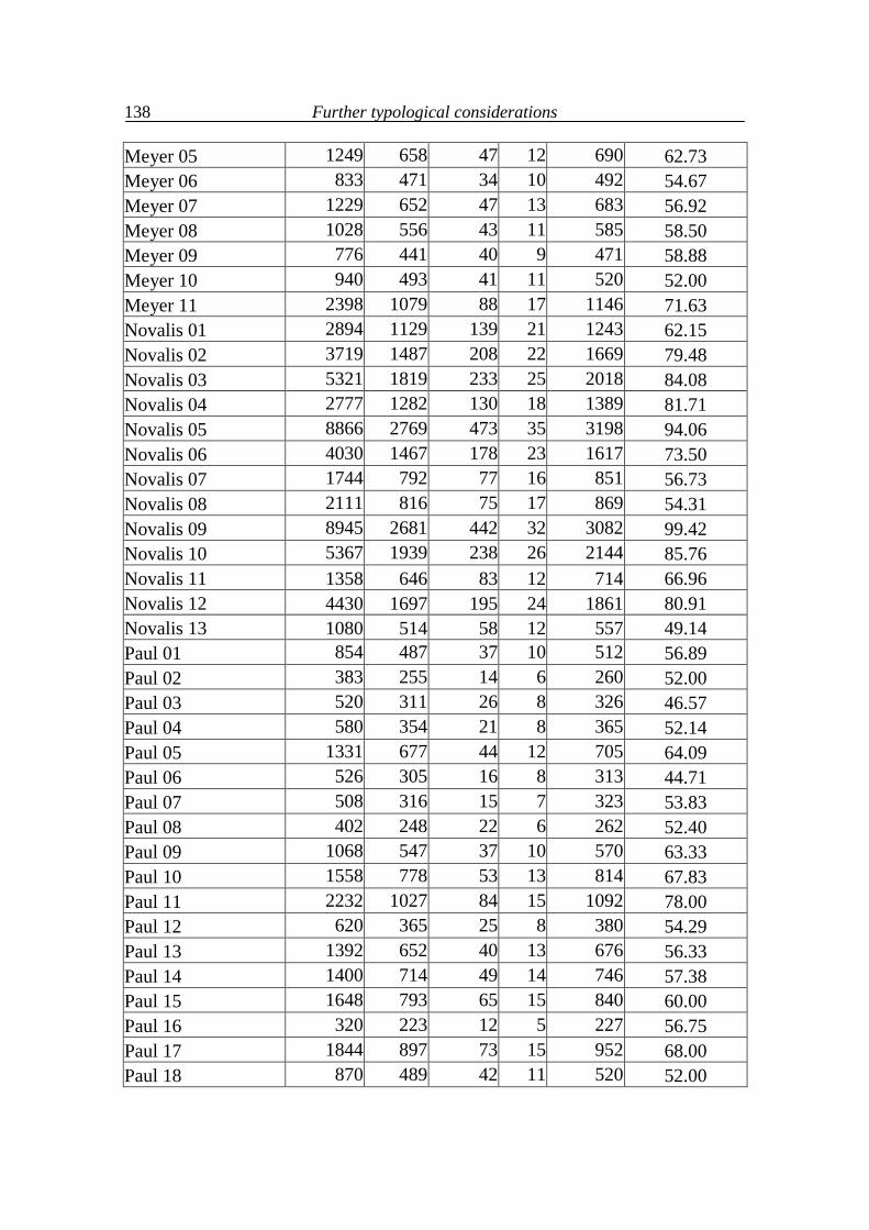
Further typological considerations

138

Meyer 05 1249 658 47 12 690 62.73 Meyer 06 833 471 34 10 492 54.67 Meyer 07 1229 652 47 13 683 56.92 Meyer 08 1028 556 43 11 585 58.50 Meyer 09 776 441 40 9 471 58.88 Meyer 10 940 493 41 11 520 52.00 Meyer 11 2398 1079 88 17 1146 71.63 Novalis 01 2894 1129 139 21 1243 62.15 Novalis 02 3719 1487 208 22 1669 79.48 Novalis 03 5321 1819 233 25 2018 84.08 Novalis 04 2777 1282 130 18 1389 81.71 Novalis 05 8866 2769 473 35 3198 94.06 Novalis 06 4030 1467 178 23 1617 73.50 Novalis 07 1744 792 77 16 851 56.73 Novalis 08 2111 816 75 17 869 54.31 Novalis 09 8945 2681 442 32 3082 99.42 Novalis 10 5367 1939 238 26 2144 85.76 Novalis 11 1358 646 83 12 714 66.96 Novalis 12 4430 1697 195 24 1861 80.91 Novalis 13 1080 514 58 12 557 49.14 Paul 01 854 487 37 10 512 56.89 Paul 02 383 255 14 6 260 52.00 Paul 03 520 311 26 8 326 46.57 Paul 04 580 354 21 8 365 52.14 Paul 05 1331 677 44 12 705 64.09 Paul 06 526 305 16 8 313 44.71 Paul 07 508 316 15 7 323 53.83 Paul 08 402 248 22 6 262 52.40 Paul 09 1068 547 37 10 570 63.33 Paul 10 1558 778 53 13 814 67.83 Paul 11 2232 1027 84 15 1092 78.00 Paul 12 620 365 25 8 380 54.29 Paul 13 1392 652 40 13 676 56.33 Paul 14 1400 714 49 14 746 57.38 Paul 15 1648 793 65 15 840 60.00 Paul 16 320 223 12 5 227 56.75 Paul 17 1844 897 73 15 952 68.00 Paul 18 870 489 42 11 520 52.00

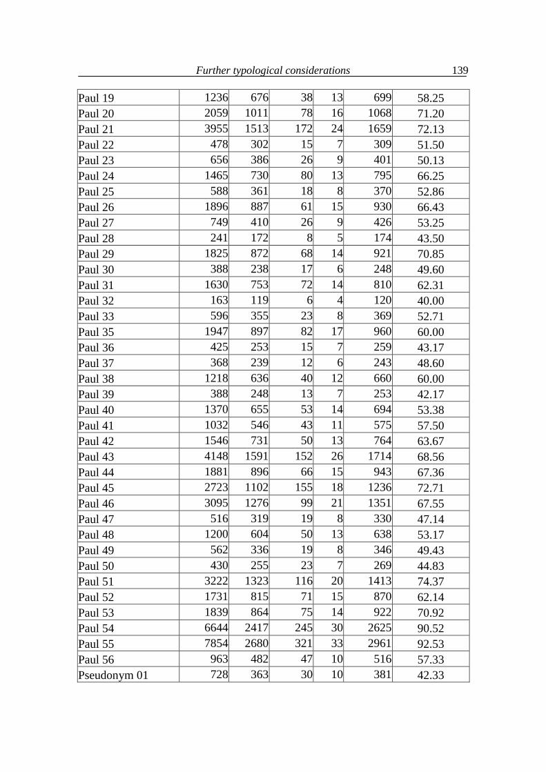
Further typological considerations

139

Paul 19 1236 676 38 13 699 58.25 Paul 20 2059 1011 78 16 1068 71.20 Paul 21 3955 1513 172 24 1659 72.13 Paul 22 478 302 15 7 309 51.50 Paul 23 656 386 26 9 401 50.13 Paul 24 1465 730 80 13 795 66.25 Paul 25 588 361 18 8 370 52.86 Paul 26 1896 887 61 15 930 66.43 Paul 27 749 410 26 9 426 53.25 Paul 28 241 172 8 5 174 43.50 Paul 29 1825 872 68 14 921 70.85 Paul 30 388 238 17 6 248 49.60 Paul 31 1630 753 72 14 810 62.31 Paul 32 163 119 6 4 120 40.00 Paul 33 596 355 23 8 369 52.71 Paul 35 1947 897 82 17 960 60.00 Paul 36 425 253 15 7 259 43.17 Paul 37 368 239 12 6 243 48.60 Paul 38 1218 636 40 12 660 60.00 Paul 39 388 248 13 7 253 42.17 Paul 40 1370 655 53 14 694 53.38 Paul 41 1032 546 43 11 575 57.50 Paul 42 1546 731 50 13 764 63.67 Paul 43 4148 1591 152 26 1714 68.56 Paul 44 1881 896 66 15 943 67.36 Paul 45 2723 1102 155 18 1236 72.71 Paul 46 3095 1276 99 21 1351 67.55 Paul 47 516 319 19 8 330 47.14 Paul 48 1200 604 50 13 638 53.17 Paul 49 562 336 19 8 346 49.43 Paul 50 430 255 23 7 269 44.83 Paul 51 3222 1323 116 20 1413 74.37 Paul 52 1731 815 71 15 870 62.14 Paul 53 1839 864 75 14 922 70.92 Paul 54 6644 2417 245 30 2625 90.52 Paul 55 7854 2680 321 33 2961 92.53 Paul 56 963 482 47 10 516 57.33 Pseudonym 01 728 363 30 10 381 42.33

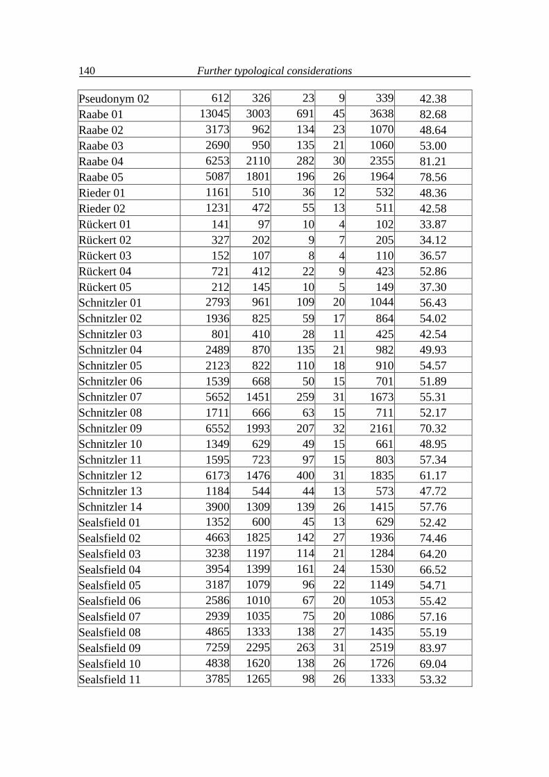
Further typological considerations

140

Pseudonym 02 612 326 23 9 339 42.38 Raabe 01 13045 3003 691 45 3638 82.68 Raabe 02 3173 962 134 23 1070 48.64 Raabe 03 2690 950 135 21 1060 53.00 Raabe 04 6253 2110 282 30 2355 81.21 Raabe 05 5087 1801 196 26 1964 78.56 Rieder 01 1161 510 36 12 532 48.36 Rieder 02 1231 472 55 13 511 42.58 Rückert 01 141 97 10 4 102 33.87 Rückert 02 327 202 9 7 205 34.12 Rückert 03 152 107 8 4 110 36.57 Rückert 04 721 412 22 9 423 52.86 Rückert 05 212 145 10 5 149 37.30 Schnitzler 01 2793 961 109 20 1044 56.43 Schnitzler 02 1936 825 59 17 864 54.02 Schnitzler 03 801 410 28 11 425 42.54 Schnitzler 04 2489 870 135 21 982 49.93 Schnitzler 05 2123 822 110 18 910 54.57 Schnitzler 06 1539 668 50 15 701 51.89 Schnitzler 07 5652 1451 259 31 1673 55.31 Schnitzler 08 1711 666 63 15 711 52.17 Schnitzler 09 6552 1993 207 32 2161 70.32 Schnitzler 10 1349 629 49 15 661 48.95 Schnitzler 11 1595 723 97 15 803 57.34 Schnitzler 12 6173 1476 400 31 1835 61.17 Schnitzler 13 1184 544 44 13 573 47.72 Schnitzler 14 3900 1309 139 26 1415 57.76 Sealsfield 01 1352 600 45 13 629 52.42 Sealsfield 02 4663 1825 142 27 1936 74.46 Sealsfield 03 3238 1197 114 21 1284 64.20 Sealsfield 04 3954 1399 161 24 1530 66.52 Sealsfield 05 3187 1079 96 22 1149 54.71 Sealsfield 06 2586 1010 67 20 1053 55.42 Sealsfield 07 2939 1035 75 20 1086 57.16 Sealsfield 08 4865 1333 138 27 1435 55.19 Sealsfield 09 7259 2295 263 31 2519 83.97 Sealsfield 10 4838 1620 138 26 1726 69.04 Sealsfield 11 3785 1265 98 26 1333 53.32

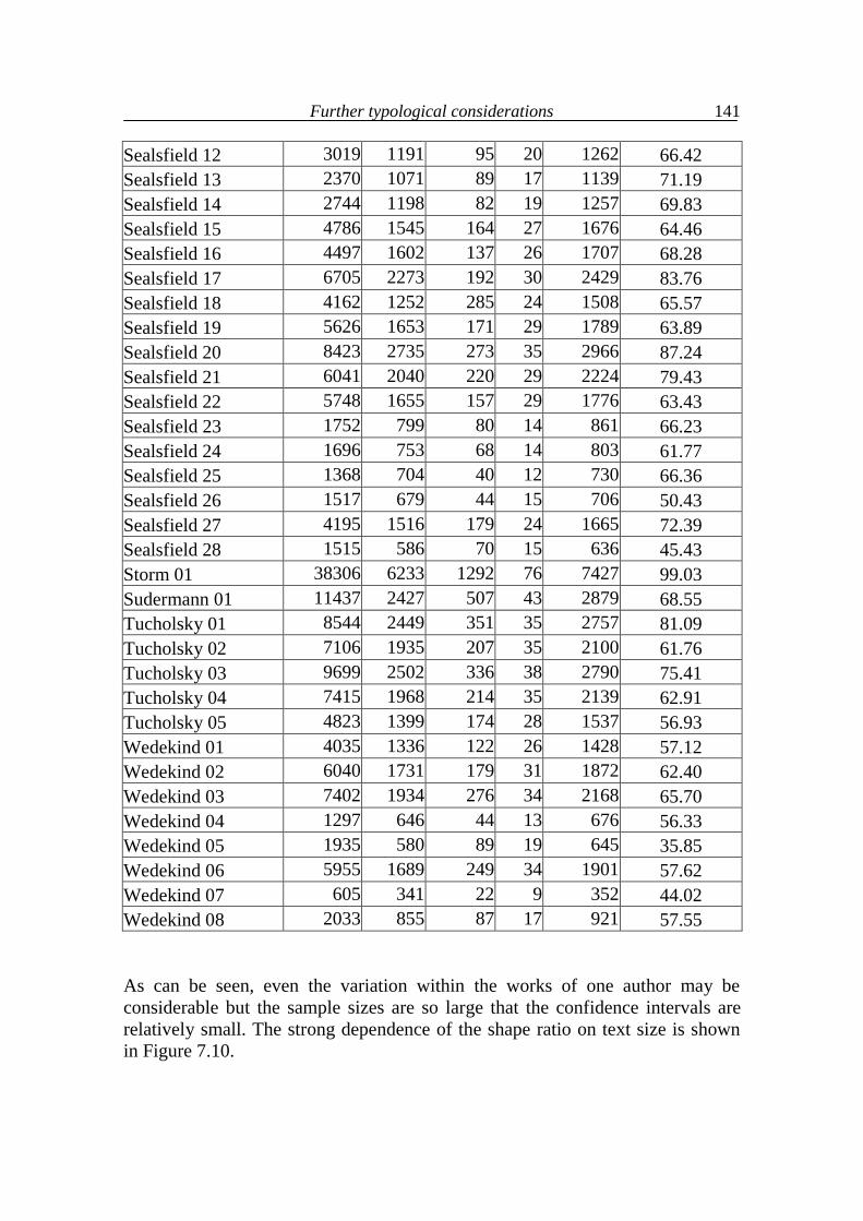
Further typological considerations

141

Sealsfield 12 3019 1191 95 20 1262 66.42 Sealsfield 13 2370 1071 89 17 1139 71.19 Sealsfield 14 2744 1198 82 19 1257 69.83 Sealsfield 15 4786 1545 164 27 1676 64.46 Sealsfield 16 4497 1602 137 26 1707 68.28 Sealsfield 17 6705 2273 192 30 2429 83.76 Sealsfield 18 4162 1252 285 24 1508 65.57 Sealsfield 19 5626 1653 171 29 1789 63.89 Sealsfield 20 8423 2735 273 35 2966 87.24 Sealsfield 21 6041 2040 220 29 2224 79.43 Sealsfield 22 5748 1655 157 29 1776 63.43 Sealsfield 23 1752 799 80 14 861 66.23 Sealsfield 24 1696 753 68 14 803 61.77 Sealsfield 25 1368 704 40 12 730 66.36 Sealsfield 26 1517 679 44 15 706 50.43 Sealsfield 27 4195 1516 179 24 1665 72.39 Sealsfield 28 1515 586 70 15 636 45.43 Storm 01 38306 6233 1292 76 7427 99.03 Sudermann 01 11437 2427 507 43 2879 68.55 Tucholsky 01 8544 2449 351 35 2757 81.09 Tucholsky 02 7106 1935 207 35 2100 61.76 Tucholsky 03 9699 2502 336 38 2790 75.41 Tucholsky 04 7415 1968 214 35 2139 62.91 Tucholsky 05 4823 1399 174 28 1537 56.93 Wedekind 01 4035 1336 122 26 1428 57.12 Wedekind 02 6040 1731 179 31 1872 62.40 Wedekind 03 7402 1934 276 34 2168 65.70 Wedekind 04 1297 646 44 13 676 56.33 Wedekind 05 1935 580 89 19 645 35.85 Wedekind 06 5955 1689 249 34 1901 57.62 Wedekind 07 605 341 22 9 352 44.02 Wedekind 08 2033 855 87 17 921 57.55

As can be seen, even the variation within the works of one author may be considerable but the sample sizes are so large that the confidence intervals are relatively small. The strong dependence of the shape ratio on text size is shown in Figure 7.10.

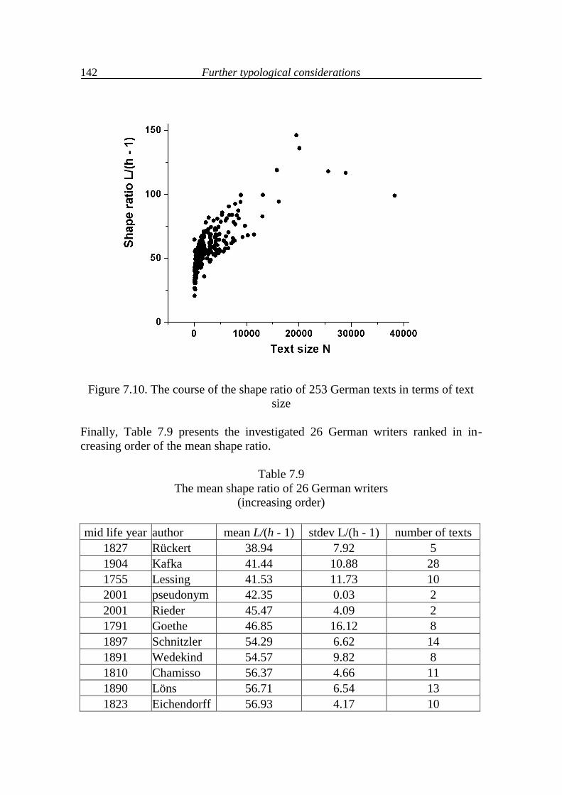
Further typological considerations

142

Figure 7.10. The course of the shape ratio of 253 German texts in terms of text size

Finally, Table 7.9 presents the investigated 26 German writers ranked in in-creasing order of the mean shape ratio.

Table 7.9 The mean shape ratio of 26 German writers

(increasing order)

mid life year author mean L/(h - 1) stdev L/(h - 1) number of texts 1827 Rückert 38.94 7.92 5 1904 Kafka 41.44 10.88 28 1755 Lessing 41.53 11.73 10 2001 pseudonym 42.35 0.03 2 2001 Rieder 45.47 4.09 2 1791 Goethe 46.85 16.12 8 1897 Schnitzler 54.29 6.62 14 1891 Wedekind 54.57 9.82 8 1810 Chamisso 56.37 4.66 11 1890 Löns 56.71 6.54 13 1823 Eichendorff 56.93 4.17 10

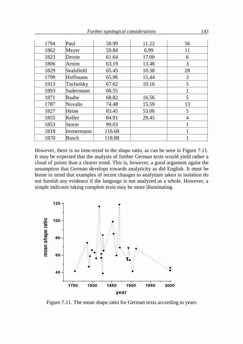
Further typological considerations

143

1794 Paul 58.99 11.22 56 1862 Meyer 59.84 6.99 11 1823 Droste 61.64 17.00 6 1806 Arnim 63.19 13.48 3 1829 Sealsfield 65.45 10.38 28 1799 Hoffmann 65.96 15.44 3 1913 Tucholsky 67.62 10.16 5 1893 Sudermann 68.55 1 1871 Raabe 68.82 16.56 5 1787 Novalis 74.48 15.59 13 1827 Heine 83.45 53.06 5 1855 Keller 84.91 29.45 4 1853 Storm 99.03 1 1818 Immermann 116.68 1 1870 Busch 118.88 1

However, there is no time-trend in the shape ratio, as can be seen in Figure 7.11. It may be expected that the analysis of further German texts would yield rather a cloud of points than a clearer trend. This is, however, a good argument agaist the assumption that German develops towards analyticity as did English. It must be borne in mind that examples of recent changes to analytism taken in isolation do not furnish any evidence if the language is not analyzed as a whole. However, a simple indicator taking complete texts may be more illuminating.

Figure 7.11. The mean shape ratio for German texts according to years

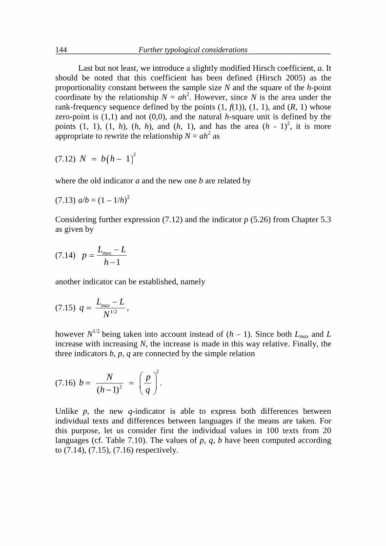
Further typological considerations

144

Last but not least, we introduce a slightly modified Hirsch coefficient, a. It should be noted that this coefficient has been defined (Hirsch 2005) as the proportionality constant between the sample size N and the square of the h-point coordinate by the relationship N = ah2. However, since N is the area under the rank-frequency sequence defined by the points (1, f(1)), (1, 1), and (R, 1) whose zero-point is (1,1) and not (0,0), and the natural h-square unit is defined by the points (1, 1), (1, h), (h, h), and (h, 1), and has the area (h - 1)2, it is more appropriate to rewrite the relationship N = ah2 as (7.12) 2 – 1N b h where the old indicator a and the new one b are related by (7.13) a/b = (1 – 1/h)2 Considering further expression (7.12) and the indicator p (5.26) from Chapter 5.3 as given by

(7.14) max

1L Lp

h

another indicator can be established, namely

(7.15) 1/2maxL LqN

,

however N1/2 being taken into account instead of (h – 1). Since both Lmax and L increase with increasing N, the increase is made in this way relative. Finally, the three indicators b, p, q are connected by the simple relation

(7.16) 2

2 ( 1)

N pbh q

.

Unlike p, the new q-indicator is able to express both differences between individual texts and differences between languages if the means are taken. For this purpose, let us consider first the individual values in 100 texts from 20 languages (cf. Table 7.10). The values of p, q, b have been computed according to (7.14), (7.15), (7.16) respectively.

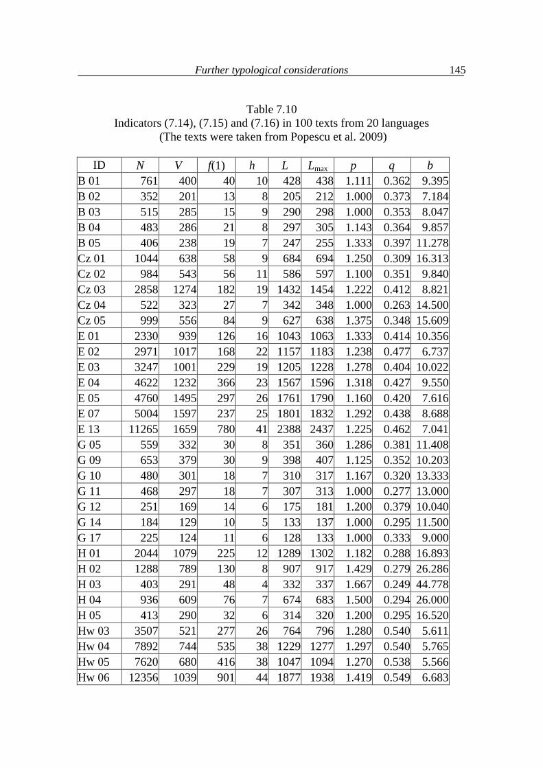
Further typological considerations

145

Table 7.10

Indicators (7.14), (7.15) and (7.16) in 100 texts from 20 languages (The texts were taken from Popescu et al. 2009)

ID N V f(1) h L Lmax p q b

B 01 761 400 40 10 428 438 1.111 0.362 9.395 B 02 352 201 13 8 205 212 1.000 0.373 7.184 B 03 515 285 15 9 290 298 1.000 0.353 8.047 B 04 483 286 21 8 297 305 1.143 0.364 9.857 B 05 406 238 19 7 247 255 1.333 0.397 11.278 Cz 01 1044 638 58 9 684 694 1.250 0.309 16.313 Cz 02 984 543 56 11 586 597 1.100 0.351 9.840 Cz 03 2858 1274 182 19 1432 1454 1.222 0.412 8.821 Cz 04 522 323 27 7 342 348 1.000 0.263 14.500 Cz 05 999 556 84 9 627 638 1.375 0.348 15.609 E 01 2330 939 126 16 1043 1063 1.333 0.414 10.356 E 02 2971 1017 168 22 1157 1183 1.238 0.477 6.737 E 03 3247 1001 229 19 1205 1228 1.278 0.404 10.022 E 04 4622 1232 366 23 1567 1596 1.318 0.427 9.550 E 05 4760 1495 297 26 1761 1790 1.160 0.420 7.616 E 07 5004 1597 237 25 1801 1832 1.292 0.438 8.688 E 13 11265 1659 780 41 2388 2437 1.225 0.462 7.041 G 05 559 332 30 8 351 360 1.286 0.381 11.408 G 09 653 379 30 9 398 407 1.125 0.352 10.203 G 10 480 301 18 7 310 317 1.167 0.320 13.333 G 11 468 297 18 7 307 313 1.000 0.277 13.000 G 12 251 169 14 6 175 181 1.200 0.379 10.040 G 14 184 129 10 5 133 137 1.000 0.295 11.500 G 17 225 124 11 6 128 133 1.000 0.333 9.000 H 01 2044 1079 225 12 1289 1302 1.182 0.288 16.893 H 02 1288 789 130 8 907 917 1.429 0.279 26.286 H 03 403 291 48 4 332 337 1.667 0.249 44.778 H 04 936 609 76 7 674 683 1.500 0.294 26.000 H 05 413 290 32 6 314 320 1.200 0.295 16.520 Hw 03 3507 521 277 26 764 796 1.280 0.540 5.611 Hw 04 7892 744 535 38 1229 1277 1.297 0.540 5.765 Hw 05 7620 680 416 38 1047 1094 1.270 0.538 5.566 Hw 06 12356 1039 901 44 1877 1938 1.419 0.549 6.683

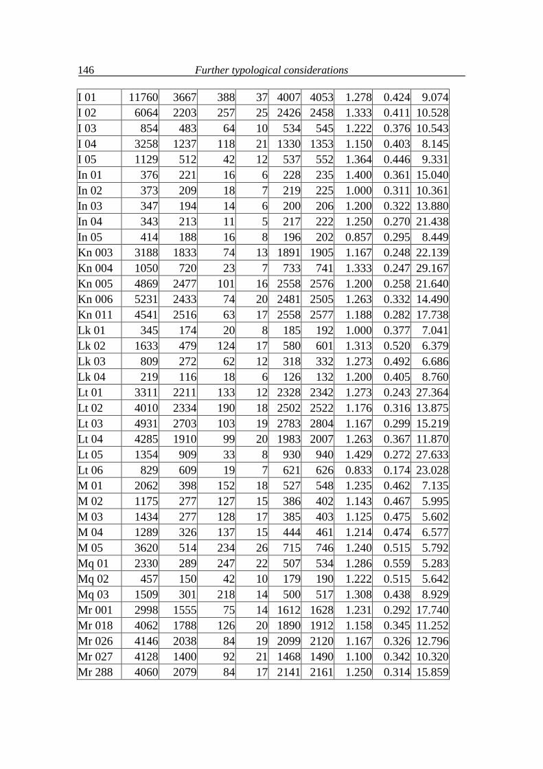
Further typological considerations

146

I 01 11760 3667 388 37 4007 4053 1.278 0.424 9.074 I 02 6064 2203 257 25 2426 2458 1.333 0.411 10.528 I 03 854 483 64 10 534 545 1.222 0.376 10.543 I 04 3258 1237 118 21 1330 1353 1.150 0.403 8.145 I 05 1129 512 42 12 537 552 1.364 0.446 9.331 In 01 376 221 16 6 228 235 1.400 0.361 15.040 In 02 373 209 18 7 219 225 1.000 0.311 10.361 In 03 347 194 14 6 200 206 1.200 0.322 13.880 In 04 343 213 11 5 217 222 1.250 0.270 21.438 In 05 414 188 16 8 196 202 0.857 0.295 8.449 Kn 003 3188 1833 74 13 1891 1905 1.167 0.248 22.139 Kn 004 1050 720 23 7 733 741 1.333 0.247 29.167 Kn 005 4869 2477 101 16 2558 2576 1.200 0.258 21.640 Kn 006 5231 2433 74 20 2481 2505 1.263 0.332 14.490 Kn 011 4541 2516 63 17 2558 2577 1.188 0.282 17.738 Lk 01 345 174 20 8 185 192 1.000 0.377 7.041 Lk 02 1633 479 124 17 580 601 1.313 0.520 6.379 Lk 03 809 272 62 12 318 332 1.273 0.492 6.686 Lk 04 219 116 18 6 126 132 1.200 0.405 8.760 Lt 01 3311 2211 133 12 2328 2342 1.273 0.243 27.364 Lt 02 4010 2334 190 18 2502 2522 1.176 0.316 13.875 Lt 03 4931 2703 103 19 2783 2804 1.167 0.299 15.219 Lt 04 4285 1910 99 20 1983 2007 1.263 0.367 11.870 Lt 05 1354 909 33 8 930 940 1.429 0.272 27.633 Lt 06 829 609 19 7 621 626 0.833 0.174 23.028 M 01 2062 398 152 18 527 548 1.235 0.462 7.135 M 02 1175 277 127 15 386 402 1.143 0.467 5.995 M 03 1434 277 128 17 385 403 1.125 0.475 5.602 M 04 1289 326 137 15 444 461 1.214 0.474 6.577 M 05 3620 514 234 26 715 746 1.240 0.515 5.792 Mq 01 2330 289 247 22 507 534 1.286 0.559 5.283 Mq 02 457 150 42 10 179 190 1.222 0.515 5.642 Mq 03 1509 301 218 14 500 517 1.308 0.438 8.929 Mr 001 2998 1555 75 14 1612 1628 1.231 0.292 17.740 Mr 018 4062 1788 126 20 1890 1912 1.158 0.345 11.252 Mr 026 4146 2038 84 19 2099 2120 1.167 0.326 12.796 Mr 027 4128 1400 92 21 1468 1490 1.100 0.342 10.320 Mr 288 4060 2079 84 17 2141 2161 1.250 0.314 15.859

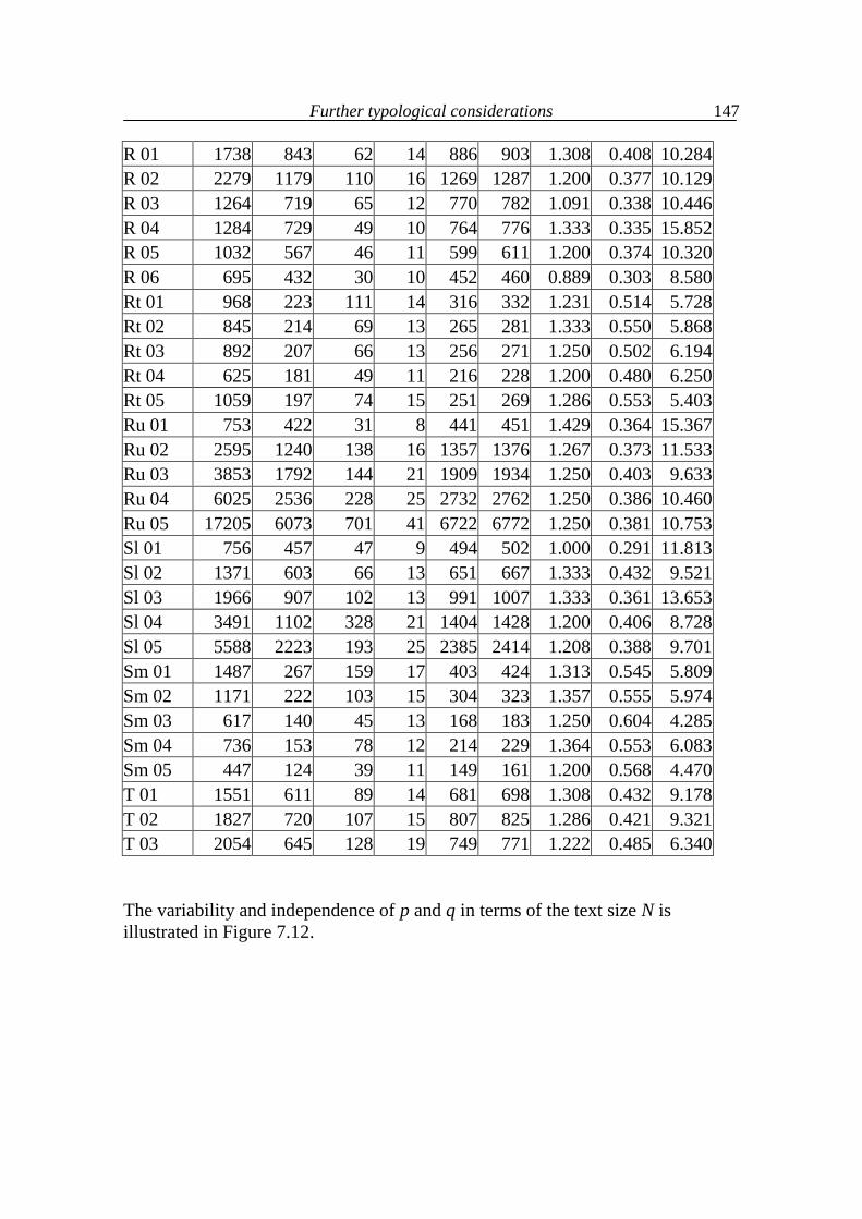
Further typological considerations

147

R 01 1738 843 62 14 886 903 1.308 0.408 10.284 R 02 2279 1179 110 16 1269 1287 1.200 0.377 10.129 R 03 1264 719 65 12 770 782 1.091 0.338 10.446 R 04 1284 729 49 10 764 776 1.333 0.335 15.852 R 05 1032 567 46 11 599 611 1.200 0.374 10.320 R 06 695 432 30 10 452 460 0.889 0.303 8.580 Rt 01 968 223 111 14 316 332 1.231 0.514 5.728 Rt 02 845 214 69 13 265 281 1.333 0.550 5.868 Rt 03 892 207 66 13 256 271 1.250 0.502 6.194 Rt 04 625 181 49 11 216 228 1.200 0.480 6.250 Rt 05 1059 197 74 15 251 269 1.286 0.553 5.403 Ru 01 753 422 31 8 441 451 1.429 0.364 15.367 Ru 02 2595 1240 138 16 1357 1376 1.267 0.373 11.533 Ru 03 3853 1792 144 21 1909 1934 1.250 0.403 9.633 Ru 04 6025 2536 228 25 2732 2762 1.250 0.386 10.460 Ru 05 17205 6073 701 41 6722 6772 1.250 0.381 10.753 Sl 01 756 457 47 9 494 502 1.000 0.291 11.813 Sl 02 1371 603 66 13 651 667 1.333 0.432 9.521 Sl 03 1966 907 102 13 991 1007 1.333 0.361 13.653 Sl 04 3491 1102 328 21 1404 1428 1.200 0.406 8.728 Sl 05 5588 2223 193 25 2385 2414 1.208 0.388 9.701 Sm 01 1487 267 159 17 403 424 1.313 0.545 5.809 Sm 02 1171 222 103 15 304 323 1.357 0.555 5.974 Sm 03 617 140 45 13 168 183 1.250 0.604 4.285 Sm 04 736 153 78 12 214 229 1.364 0.553 6.083 Sm 05 447 124 39 11 149 161 1.200 0.568 4.470 T 01 1551 611 89 14 681 698 1.308 0.432 9.178 T 02 1827 720 107 15 807 825 1.286 0.421 9.321 T 03 2054 645 128 19 749 771 1.222 0.485 6.340 The variability and independence of p and q in terms of the text size N is illustrated in Figure 7.12.

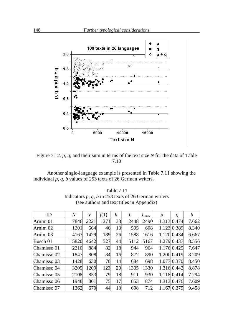
Further typological considerations

148

Figure 7.12. p, q, and their sum in terms of the text size N for the data of Table 7.10

Another single-language example is presented in Table 7.11 showing the

individual p, q, b values of 253 texts of 26 German writers.

Table 7.11 Indicators p, q, b in 253 texts of 26 German writers

(see authors and text titles in Appendix)

ID N V f(1) h L Lmax p q b Arnim 01 7846 2221 271 33 2448 2490 1.313 0.474 7.662 Arnim 02 1201 564 46 13 595 608 1.123 0.389 8.340 Arnim 03 4167 1429 189 26 1588 1616 1.120 0.434 6.667 Busch 01 15820 4642 527 44 5112 5167 1.279 0.437 8.556 Chamisso 01 2210 884 82 18 944 964 1.176 0.425 7.647 Chamisso 02 1847 808 84 16 872 890 1.200 0.419 8.209 Chamisso 03 1428 630 70 14 684 698 1.077 0.370 8.450 Chamisso 04 3205 1209 123 20 1305 1330 1.316 0.442 8.878 Chamisso 05 2108 853 79 18 911 930 1.118 0.414 7.294 Chamisso 06 1948 801 75 17 853 874 1.313 0.476 7.609 Chamisso 07 1362 670 44 13 698 712 1.167 0.379 9.458

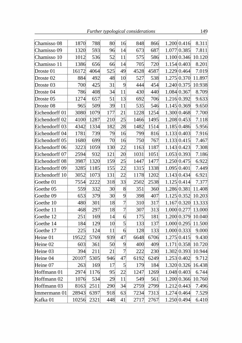
Further typological considerations

149

Chamisso 08 1870 788 80 16 848 866 1.200 0.416 8.311 Chamisso 09 1320 593 96 14 673 687 1.077 0.385 7.811 Chamisso 10 1012 536 52 11 575 586 1.100 0.346 10.120 Chamisso 11 1386 656 66 14 705 720 1.154 0.403 8.201 Droste 01 16172 4064 525 49 4528 4587 1.229 0.464 7.019 Droste 02 884 492 48 10 527 538 1.275 0.370 11.897 Droste 03 700 425 31 9 444 454 1.240 0.375 10.938 Droste 04 786 408 34 11 430 440 1.084 0.367 8.709 Droste 05 1274 657 51 13 692 706 1.216 0.392 9.633 Droste 08 965 509 39 11 535 546 1.145 0.369 9.650 Eichendorff 01 3080 1079 177 21 1228 1254 1.300 0.468 7.700 Eichendorff 02 4100 1287 210 25 1466 1495 1.208 0.453 7.118 Eichendorff 03 4342 1334 182 28 1482 1514 1.185 0.486 5.956 Eichendorff 04 1781 739 79 16 799 816 1.133 0.403 7.916 Eichendorff 05 1680 699 70 16 750 767 1.133 0.415 7.467 Eichendorff 06 3223 1059 130 22 1163 1187 1.143 0.423 7.308 Eichendorff 07 2594 932 121 20 1031 1051 1.053 0.393 7.186 Eichendorff 08 3987 1320 159 25 1447 1477 1.250 0.475 6.922 Eichendorff 09 3285 1185 155 22 1315 1338 1.095 0.401 7.449 Eichendorff 10 3052 1073 131 22 1178 1202 1.143 0.434 6.921 Goethe 01 7554 2222 318 33 2502 2538 1.125 0.414 7.377 Goethe 05 559 332 30 8 351 360 1.286 0.381 11.408 Goethe 09 653 379 30 9 398 407 1.125 0.352 10.203 Goethe 10 480 301 18 7 310 317 1.167 0.320 13.333 Goethe 11 468 297 18 7 307 313 1.000 0.277 13.000 Goethe 12 251 169 14 6 175 181 1.200 0.379 10.040 Goethe 14 184 129 10 5 133 137 1.000 0.295 11.500 Goethe 17 225 124 11 6 128 133 1.000 0.333 9.000 Heine 01 19522 5769 939 47 6648 6706 1.275 0.415 9.430 Heine 02 603 361 50 9 400 409 1.171 0.358 10.720 Heine 03 394 211 21 7 222 230 1.302 0.393 10.944 Heine 04 20107 5305 946 47 6192 6249 1.253 0.402 9.712 Heine 07 263 169 17 5 179 184 1.320 0.326 16.438 Hoffmann 01 2974 1176 95 22 1247 1269 1.048 0.403 6.744 Hoffmann 02 1076 534 29 11 549 561 1.200 0.366 10.760 Hoffmann 03 8163 2511 290 34 2759 2799 1.212 0.443 7.496 Immermann 01 28943 6397 918 63 7234 7313 1.274 0.464 7.529 Kafka 01 10256 2321 448 41 2717 2767 1.250 0.494 6.410

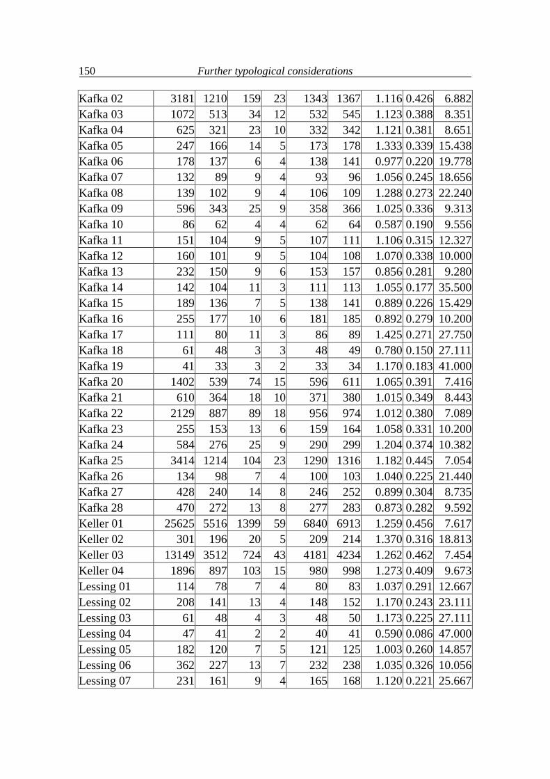
Further typological considerations

150

Kafka 02 3181 1210 159 23 1343 1367 1.116 0.426 6.882 Kafka 03 1072 513 34 12 532 545 1.123 0.388 8.351 Kafka 04 625 321 23 10 332 342 1.121 0.381 8.651 Kafka 05 247 166 14 5 173 178 1.333 0.339 15.438 Kafka 06 178 137 6 4 138 141 0.977 0.220 19.778 Kafka 07 132 89 9 4 93 96 1.056 0.245 18.656 Kafka 08 139 102 9 4 106 109 1.288 0.273 22.240 Kafka 09 596 343 25 9 358 366 1.025 0.336 9.313 Kafka 10 86 62 4 4 62 64 0.587 0.190 9.556 Kafka 11 151 104 9 5 107 111 1.106 0.315 12.327 Kafka 12 160 101 9 5 104 108 1.070 0.338 10.000 Kafka 13 232 150 9 6 153 157 0.856 0.281 9.280 Kafka 14 142 104 11 3 111 113 1.055 0.177 35.500 Kafka 15 189 136 7 5 138 141 0.889 0.226 15.429 Kafka 16 255 177 10 6 181 185 0.892 0.279 10.200 Kafka 17 111 80 11 3 86 89 1.425 0.271 27.750 Kafka 18 61 48 3 3 48 49 0.780 0.150 27.111 Kafka 19 41 33 3 2 33 34 1.170 0.183 41.000 Kafka 20 1402 539 74 15 596 611 1.065 0.391 7.416 Kafka 21 610 364 18 10 371 380 1.015 0.349 8.443 Kafka 22 2129 887 89 18 956 974 1.012 0.380 7.089 Kafka 23 255 153 13 6 159 164 1.058 0.331 10.200 Kafka 24 584 276 25 9 290 299 1.204 0.374 10.382 Kafka 25 3414 1214 104 23 1290 1316 1.182 0.445 7.054 Kafka 26 134 98 7 4 100 103 1.040 0.225 21.440 Kafka 27 428 240 14 8 246 252 0.899 0.304 8.735 Kafka 28 470 272 13 8 277 283 0.873 0.282 9.592 Keller 01 25625 5516 1399 59 6840 6913 1.259 0.456 7.617 Keller 02 301 196 20 5 209 214 1.370 0.316 18.813 Keller 03 13149 3512 724 43 4181 4234 1.262 0.462 7.454 Keller 04 1896 897 103 15 980 998 1.273 0.409 9.673 Lessing 01 114 78 7 4 80 83 1.037 0.291 12.667 Lessing 02 208 141 13 4 148 152 1.170 0.243 23.111 Lessing 03 61 48 4 3 48 50 1.173 0.225 27.111 Lessing 04 47 41 2 2 40 41 0.590 0.086 47.000 Lessing 05 182 120 7 5 121 125 1.003 0.260 14.857 Lessing 06 362 227 13 7 232 238 1.035 0.326 10.056 Lessing 07 231 161 9 4 165 168 1.120 0.221 25.667

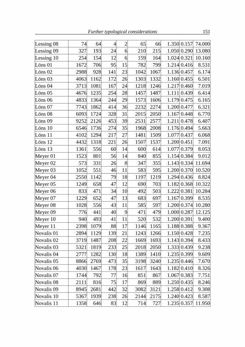
Further typological considerations

151

Lessing 08 74 64 4 2 65 66 1.350 0.157 74.000 Lessing 09 327 193 24 6 210 215 1.050 0.290 13.080 Lessing 10 254 154 12 6 159 164 1.024 0.321 10.160 Löns 01 1672 706 95 15 782 799 1.214 0.416 8.531 Löns 02 2988 928 141 23 1042 1067 1.136 0.457 6.174 Löns 03 4063 1162 172 26 1303 1332 1.160 0.455 6.501 Löns 04 3713 1081 167 24 1218 1246 1.217 0.460 7.019 Löns 05 4676 1235 254 28 1457 1487 1.111 0.439 6.414 Löns 06 4833 1364 244 29 1573 1606 1.179 0.475 6.165 Löns 07 7743 1862 414 36 2232 2274 1.200 0.477 6.321 Löns 08 6093 1724 328 31 2015 2050 1.167 0.448 6.770 Löns 09 9252 2126 453 39 2531 2577 1.211 0.478 6.407 Löns 10 6546 1736 274 35 1968 2008 1.176 0.494 5.663 Löns 11 4102 1294 217 27 1481 1509 1.077 0.437 6.068 Löns 12 4432 1318 221 26 1507 1537 1.200 0.451 7.091 Löns 13 1361 556 60 14 600 614 1.077 0.379 8.053 Meyer 01 1523 801 56 14 840 855 1.154 0.384 9.012 Meyer 02 573 331 26 8 347 355 1.143 0.334 11.694 Meyer 03 1052 551 46 11 583 595 1.200 0.370 10.520 Meyer 04 2550 1142 79 18 1197 1219 1.294 0.436 8.824 Meyer 05 1249 658 47 12 690 703 1.182 0.368 10.322 Meyer 06 833 471 34 10 492 503 1.222 0.381 10.284 Meyer 07 1229 652 47 13 683 697 1.167 0.399 8.535 Meyer 08 1028 556 43 11 585 597 1.200 0.374 10.280 Meyer 09 776 441 40 9 471 479 1.000 0.287 12.125 Meyer 10 940 493 41 11 520 532 1.200 0.391 9.400 Meyer 11 2398 1079 88 17 1146 1165 1.188 0.388 9.367 Novalis 01 2894 1129 139 21 1243 1266 1.150 0.428 7.235 Novalis 02 3719 1487 208 22 1669 1693 1.143 0.394 8.433 Novalis 03 5321 1819 233 25 2018 2050 1.333 0.439 9.238 Novalis 04 2777 1282 130 18 1389 1410 1.235 0.399 9.609 Novalis 05 8866 2769 473 35 3198 3240 1.235 0.446 7.670 Novalis 06 4030 1467 178 23 1617 1643 1.182 0.410 8.326 Novalis 07 1744 792 77 16 851 867 1.067 0.383 7.751 Novalis 08 2111 816 75 17 869 889 1.250 0.435 8.246 Novalis 09 8945 2681 442 32 3082 3121 1.258 0.412 9.308 Novalis 10 5367 1939 238 26 2144 2175 1.240 0.423 8.587 Novalis 11 1358 646 83 12 714 727 1.235 0.357 11.950

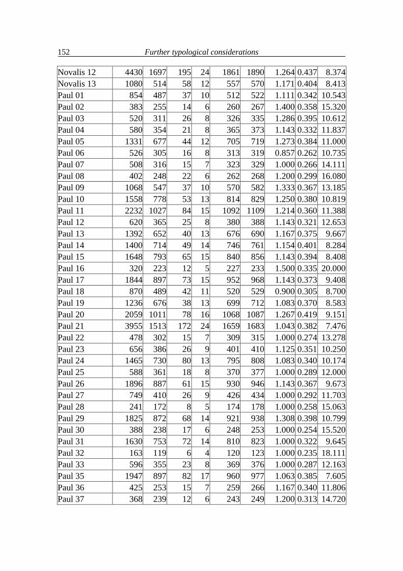
Further typological considerations

152

Novalis 12 4430 1697 195 24 1861 1890 1.264 0.437 8.374 Novalis 13 1080 514 58 12 557 570 1.171 0.404 8.413 Paul 01 854 487 37 10 512 522 1.111 0.342 10.543 Paul 02 383 255 14 6 260 267 1.400 0.358 15.320 Paul 03 520 311 26 8 326 335 1.286 0.395 10.612 Paul 04 580 354 21 8 365 373 1.143 0.332 11.837 Paul 05 1331 677 44 12 705 719 1.273 0.384 11.000 Paul 06 526 305 16 8 313 319 0.857 0.262 10.735 Paul 07 508 316 15 7 323 329 1.000 0.266 14.111 Paul 08 402 248 22 6 262 268 1.200 0.299 16.080 Paul 09 1068 547 37 10 570 582 1.333 0.367 13.185 Paul 10 1558 778 53 13 814 829 1.250 0.380 10.819 Paul 11 2232 1027 84 15 1092 1109 1.214 0.360 11.388 Paul 12 620 365 25 8 380 388 1.143 0.321 12.653 Paul 13 1392 652 40 13 676 690 1.167 0.375 9.667 Paul 14 1400 714 49 14 746 761 1.154 0.401 8.284 Paul 15 1648 793 65 15 840 856 1.143 0.394 8.408 Paul 16 320 223 12 5 227 233 1.500 0.335 20.000 Paul 17 1844 897 73 15 952 968 1.143 0.373 9.408 Paul 18 870 489 42 11 520 529 0.900 0.305 8.700 Paul 19 1236 676 38 13 699 712 1.083 0.370 8.583 Paul 20 2059 1011 78 16 1068 1087 1.267 0.419 9.151 Paul 21 3955 1513 172 24 1659 1683 1.043 0.382 7.476 Paul 22 478 302 15 7 309 315 1.000 0.274 13.278 Paul 23 656 386 26 9 401 410 1.125 0.351 10.250 Paul 24 1465 730 80 13 795 808 1.083 0.340 10.174 Paul 25 588 361 18 8 370 377 1.000 0.289 12.000 Paul 26 1896 887 61 15 930 946 1.143 0.367 9.673 Paul 27 749 410 26 9 426 434 1.000 0.292 11.703 Paul 28 241 172 8 5 174 178 1.000 0.258 15.063 Paul 29 1825 872 68 14 921 938 1.308 0.398 10.799 Paul 30 388 238 17 6 248 253 1.000 0.254 15.520 Paul 31 1630 753 72 14 810 823 1.000 0.322 9.645 Paul 32 163 119 6 4 120 123 1.000 0.235 18.111 Paul 33 596 355 23 8 369 376 1.000 0.287 12.163 Paul 35 1947 897 82 17 960 977 1.063 0.385 7.605 Paul 36 425 253 15 7 259 266 1.167 0.340 11.806 Paul 37 368 239 12 6 243 249 1.200 0.313 14.720

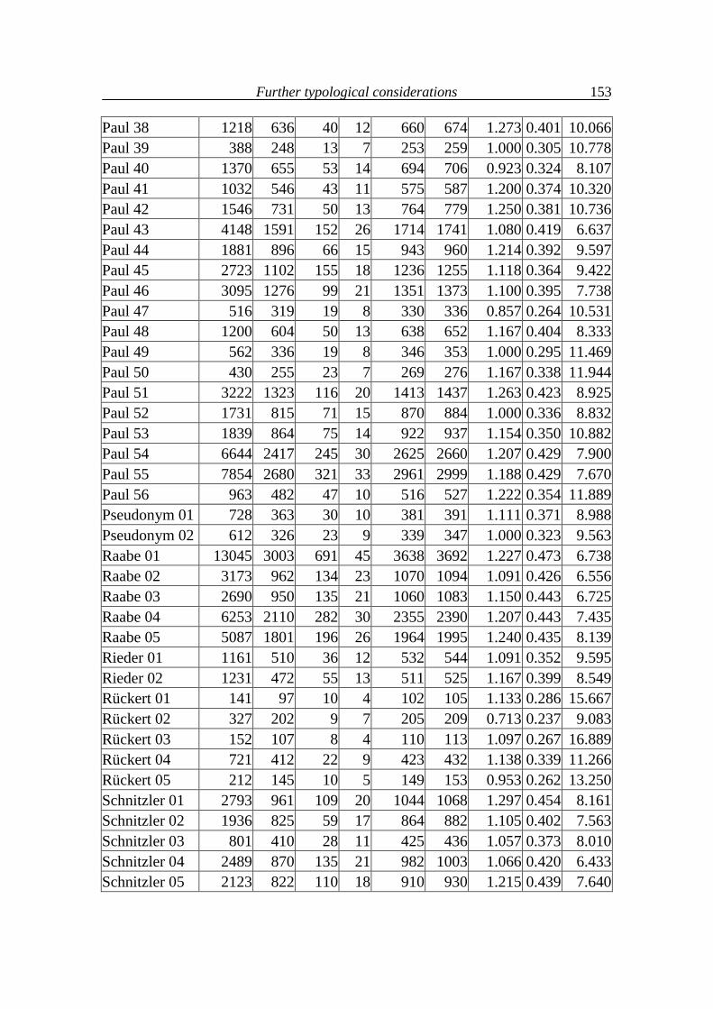
Further typological considerations

153

Paul 38 1218 636 40 12 660 674 1.273 0.401 10.066 Paul 39 388 248 13 7 253 259 1.000 0.305 10.778 Paul 40 1370 655 53 14 694 706 0.923 0.324 8.107 Paul 41 1032 546 43 11 575 587 1.200 0.374 10.320 Paul 42 1546 731 50 13 764 779 1.250 0.381 10.736 Paul 43 4148 1591 152 26 1714 1741 1.080 0.419 6.637 Paul 44 1881 896 66 15 943 960 1.214 0.392 9.597 Paul 45 2723 1102 155 18 1236 1255 1.118 0.364 9.422 Paul 46 3095 1276 99 21 1351 1373 1.100 0.395 7.738 Paul 47 516 319 19 8 330 336 0.857 0.264 10.531 Paul 48 1200 604 50 13 638 652 1.167 0.404 8.333 Paul 49 562 336 19 8 346 353 1.000 0.295 11.469 Paul 50 430 255 23 7 269 276 1.167 0.338 11.944 Paul 51 3222 1323 116 20 1413 1437 1.263 0.423 8.925 Paul 52 1731 815 71 15 870 884 1.000 0.336 8.832 Paul 53 1839 864 75 14 922 937 1.154 0.350 10.882 Paul 54 6644 2417 245 30 2625 2660 1.207 0.429 7.900 Paul 55 7854 2680 321 33 2961 2999 1.188 0.429 7.670 Paul 56 963 482 47 10 516 527 1.222 0.354 11.889 Pseudonym 01 728 363 30 10 381 391 1.111 0.371 8.988 Pseudonym 02 612 326 23 9 339 347 1.000 0.323 9.563 Raabe 01 13045 3003 691 45 3638 3692 1.227 0.473 6.738 Raabe 02 3173 962 134 23 1070 1094 1.091 0.426 6.556 Raabe 03 2690 950 135 21 1060 1083 1.150 0.443 6.725 Raabe 04 6253 2110 282 30 2355 2390 1.207 0.443 7.435 Raabe 05 5087 1801 196 26 1964 1995 1.240 0.435 8.139 Rieder 01 1161 510 36 12 532 544 1.091 0.352 9.595 Rieder 02 1231 472 55 13 511 525 1.167 0.399 8.549 Rückert 01 141 97 10 4 102 105 1.133 0.286 15.667 Rückert 02 327 202 9 7 205 209 0.713 0.237 9.083 Rückert 03 152 107 8 4 110 113 1.097 0.267 16.889 Rückert 04 721 412 22 9 423 432 1.138 0.339 11.266 Rückert 05 212 145 10 5 149 153 0.953 0.262 13.250 Schnitzler 01 2793 961 109 20 1044 1068 1.297 0.454 8.161 Schnitzler 02 1936 825 59 17 864 882 1.105 0.402 7.563 Schnitzler 03 801 410 28 11 425 436 1.057 0.373 8.010 Schnitzler 04 2489 870 135 21 982 1003 1.066 0.420 6.433 Schnitzler 05 2123 822 110 18 910 930 1.215 0.439 7.640

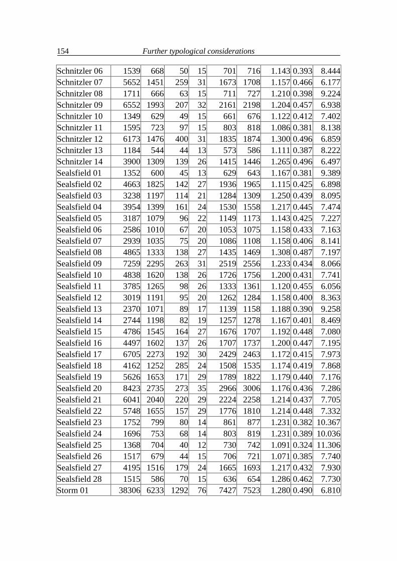
Further typological considerations

154

Schnitzler 06 1539 668 50 15 701 716 1.143 0.393 8.444 Schnitzler 07 5652 1451 259 31 1673 1708 1.157 0.466 6.177 Schnitzler 08 1711 666 63 15 711 727 1.210 0.398 9.224 Schnitzler 09 6552 1993 207 32 2161 2198 1.204 0.457 6.938 Schnitzler 10 1349 629 49 15 661 676 1.122 0.412 7.402 Schnitzler 11 1595 723 97 15 803 818 1.086 0.381 8.138 Schnitzler 12 6173 1476 400 31 1835 1874 1.300 0.496 6.859 Schnitzler 13 1184 544 44 13 573 586 1.111 0.387 8.222 Schnitzler 14 3900 1309 139 26 1415 1446 1.265 0.496 6.497 Sealsfield 01 1352 600 45 13 629 643 1.167 0.381 9.389 Sealsfield 02 4663 1825 142 27 1936 1965 1.115 0.425 6.898 Sealsfield 03 3238 1197 114 21 1284 1309 1.250 0.439 8.095 Sealsfield 04 3954 1399 161 24 1530 1558 1.217 0.445 7.474 Sealsfield 05 3187 1079 96 22 1149 1173 1.143 0.425 7.227 Sealsfield 06 2586 1010 67 20 1053 1075 1.158 0.433 7.163 Sealsfield 07 2939 1035 75 20 1086 1108 1.158 0.406 8.141 Sealsfield 08 4865 1333 138 27 1435 1469 1.308 0.487 7.197 Sealsfield 09 7259 2295 263 31 2519 2556 1.233 0.434 8.066 Sealsfield 10 4838 1620 138 26 1726 1756 1.200 0.431 7.741 Sealsfield 11 3785 1265 98 26 1333 1361 1.120 0.455 6.056 Sealsfield 12 3019 1191 95 20 1262 1284 1.158 0.400 8.363 Sealsfield 13 2370 1071 89 17 1139 1158 1.188 0.390 9.258 Sealsfield 14 2744 1198 82 19 1257 1278 1.167 0.401 8.469 Sealsfield 15 4786 1545 164 27 1676 1707 1.192 0.448 7.080 Sealsfield 16 4497 1602 137 26 1707 1737 1.200 0.447 7.195 Sealsfield 17 6705 2273 192 30 2429 2463 1.172 0.415 7.973 Sealsfield 18 4162 1252 285 24 1508 1535 1.174 0.419 7.868 Sealsfield 19 5626 1653 171 29 1789 1822 1.179 0.440 7.176 Sealsfield 20 8423 2735 273 35 2966 3006 1.176 0.436 7.286 Sealsfield 21 6041 2040 220 29 2224 2258 1.214 0.437 7.705 Sealsfield 22 5748 1655 157 29 1776 1810 1.214 0.448 7.332 Sealsfield 23 1752 799 80 14 861 877 1.231 0.382 10.367 Sealsfield 24 1696 753 68 14 803 819 1.231 0.389 10.036 Sealsfield 25 1368 704 40 12 730 742 1.091 0.324 11.306 Sealsfield 26 1517 679 44 15 706 721 1.071 0.385 7.740 Sealsfield 27 4195 1516 179 24 1665 1693 1.217 0.432 7.930 Sealsfield 28 1515 586 70 15 636 654 1.286 0.462 7.730 Storm 01 38306 6233 1292 76 7427 7523 1.280 0.490 6.810

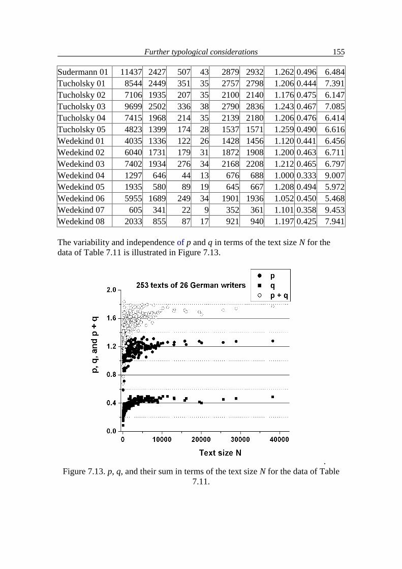
Further typological considerations

155

Sudermann 01 11437 2427 507 43 2879 2932 1.262 0.496 6.484 Tucholsky 01 8544 2449 351 35 2757 2798 1.206 0.444 7.391 Tucholsky 02 7106 1935 207 35 2100 2140 1.176 0.475 6.147 Tucholsky 03 9699 2502 336 38 2790 2836 1.243 0.467 7.085 Tucholsky 04 7415 1968 214 35 2139 2180 1.206 0.476 6.414 Tucholsky 05 4823 1399 174 28 1537 1571 1.259 0.490 6.616 Wedekind 01 4035 1336 122 26 1428 1456 1.120 0.441 6.456 Wedekind 02 6040 1731 179 31 1872 1908 1.200 0.463 6.711 Wedekind 03 7402 1934 276 34 2168 2208 1.212 0.465 6.797 Wedekind 04 1297 646 44 13 676 688 1.000 0.333 9.007 Wedekind 05 1935 580 89 19 645 667 1.208 0.494 5.972 Wedekind 06 5955 1689 249 34 1901 1936 1.052 0.450 5.468 Wedekind 07 605 341 22 9 352 361 1.101 0.358 9.453 Wedekind 08 2033 855 87 17 921 940 1.197 0.425 7.941

The variability and independence of p and q in terms of the text size N for the data of Table 7.11 is illustrated in Figure 7.13.

. Figure 7.13. p, q, and their sum in terms of the text size N for the data of Table

7.11.

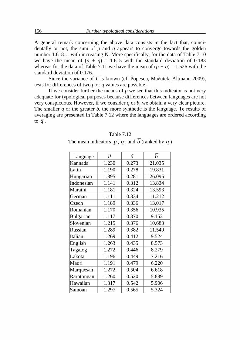
Further typological considerations

156

A general remark concerning the above data consists in the fact that, coinci-dentally or not, the sum of p and q appears to converge towards the golden number 1.618… with increasing N. More specifically, for the data of Table 7.10 we have the mean of (p + q) = 1.615 with the standard deviation of 0.183 whereas for the data of Table 7.11 we have the mean of (p + q) = 1.526 with the standard deviation of 0.176. Since the variance of L is known (cf. Popescu, Mačutek, Altmann 2009), tests for differences of two p or q values are possible. If we consider further the means of p we see that this indicator is not very adequate for typological purposes because differences between languages are not very conspicuous. However, if we consider q or b, we obtain a very clear picture. The smaller q or the greater b, the more synthetic is the language. Te results of averaging are presented in Table 7.12 where the languages are ordered according to q .

Table 7.12 The mean indicators p , q , and b (ranked by q )

Language p q b

Kannada 1.230 0.273 21.035 Latin 1.190 0.278 19.831 Hungarian 1.395 0.281 26.095 Indonesian 1.141 0.312 13.834 Marathi 1.181 0.324 13.593 German 1.111 0.334 11.212 Czech 1.189 0.336 13.017 Romanian 1.170 0.356 10.935 Bulgarian 1.117 0.370 9.152 Slovenian 1.215 0.376 10.683 Russian 1.289 0.382 11.549 Italian 1.269 0.412 9.524 English 1.263 0.435 8.573 Tagalog 1.272 0.446 8.279 Lakota 1.196 0.449 7.216 Maori 1.191 0.479 6.220 Marquesan 1.272 0.504 6.618 Rarotongan 1.260 0.520 5.889 Hawaiian 1.317 0.542 5.906 Samoan 1.297 0.565 5.324

8. Word frequency diversity and typology

In the previous chapters we saw that word form frequencies are characteristic of languages, at least in the sense that they signalize the position of language on the analytism/synthetism scale. Consequently, whatever operations we perform with word frequencies, they would reflect this property in some way. In this chapter we shall use two well known indicators, namely the entropy (H) of word frequencies and the repeat rate (RR). We shall use the Shannon entropy but the study of other kinds of entropies whose number continuously in-creases (cf. Esteban, Morales 1995) would be interesting, too. Entropy is used in linguistics for different purposes; here it is used to characterize the dispersion (non uniformity) of frequencies. The Shannon entropy is defined as

(8.1) 21

logV

r rr

H p p

,

where pr is the relative frequency of word forms, i.e. pr = fr/N for r = 1,…,V. Replacing the relative frequencies by absolute ones we obtain

(8.2) 2 21

1log logV

r rr

H N f fN

.

The variance of (8.1) is given as

(8.3) 2 22 2

1

1( ) log

V

rr

Var H p p HN

,

hence asymptotic tests are possible. Entropy lies in the interval <0, log2V> and can be normalized to <0,1> using

(8.4) 2

relHH

log V .

The values of entropy and relative entropy in individual texts are presented in Table 8.1.

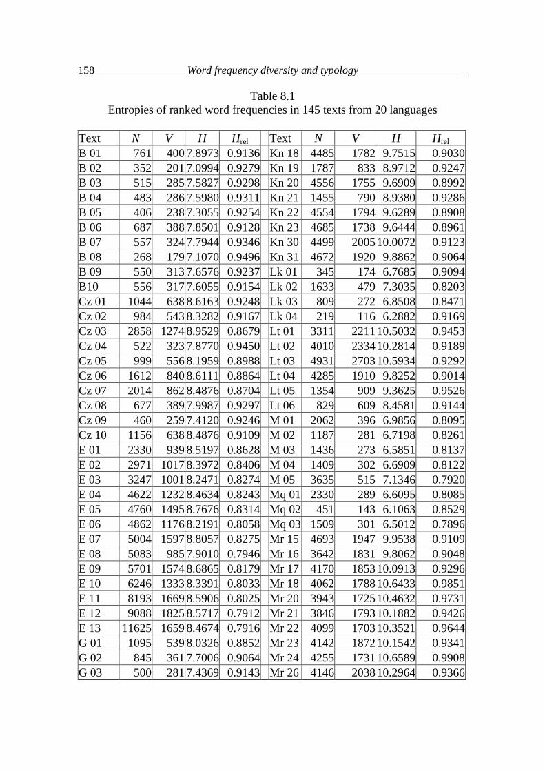
Word frequency diversity and typology

158

Table 8.1 Entropies of ranked word frequencies in 145 texts from 20 languages

Text N V H Hrel Text N V H Hrel B 01 761 400 7.8973 0.9136 Kn 18 4485 1782 9.7515 0.9030 B 02 352 201 7.0994 0.9279 Kn 19 1787 833 8.9712 0.9247 B 03 515 285 7.5827 0.9298 Kn 20 4556 1755 9.6909 0.8992 B 04 483 286 7.5980 0.9311 Kn 21 1455 790 8.9380 0.9286 B 05 406 238 7.3055 0.9254 Kn 22 4554 1794 9.6289 0.8908 B 06 687 388 7.8501 0.9128 Kn 23 4685 1738 9.6444 0.8961 B 07 557 324 7.7944 0.9346 Kn 30 4499 2005 10.0072 0.9123 B 08 268 179 7.1070 0.9496 Kn 31 4672 1920 9.8862 0.9064 B 09 550 313 7.6576 0.9237 Lk 01 345 174 6.7685 0.9094 B10 556 317 7.6055 0.9154 Lk 02 1633 479 7.3035 0.8203 Cz 01 1044 638 8.6163 0.9248 Lk 03 809 272 6.8508 0.8471 Cz 02 984 543 8.3282 0.9167 Lk 04 219 116 6.2882 0.9169 Cz 03 2858 1274 8.9529 0.8679 Lt 01 3311 2211 10.5032 0.9453 Cz 04 522 323 7.8770 0.9450 Lt 02 4010 2334 10.2814 0.9189 Cz 05 999 556 8.1959 0.8988 Lt 03 4931 2703 10.5934 0.9292 Cz 06 1612 840 8.6111 0.8864 Lt 04 4285 1910 9.8252 0.9014 Cz 07 2014 862 8.4876 0.8704 Lt 05 1354 909 9.3625 0.9526 Cz 08 677 389 7.9987 0.9297 Lt 06 829 609 8.4581 0.9144 Cz 09 460 259 7.4120 0.9246 M 01 2062 396 6.9856 0.8095 Cz 10 1156 638 8.4876 0.9109 M 02 1187 281 6.7198 0.8261 E 01 2330 939 8.5197 0.8628 M 03 1436 273 6.5851 0.8137 E 02 2971 1017 8.3972 0.8406 M 04 1409 302 6.6909 0.8122 E 03 3247 1001 8.2471 0.8274 M 05 3635 515 7.1346 0.7920 E 04 4622 1232 8.4634 0.8243 Mq 01 2330 289 6.6095 0.8085 E 05 4760 1495 8.7676 0.8314 Mq 02 451 143 6.1063 0.8529 E 06 4862 1176 8.2191 0.8058 Mq 03 1509 301 6.5012 0.7896 E 07 5004 1597 8.8057 0.8275 Mr 15 4693 1947 9.9538 0.9109 E 08 5083 985 7.9010 0.7946 Mr 16 3642 1831 9.8062 0.9048 E 09 5701 1574 8.6865 0.8179 Mr 17 4170 1853 10.0913 0.9296 E 10 6246 1333 8.3391 0.8033 Mr 18 4062 1788 10.6433 0.9851 E 11 8193 1669 8.5906 0.8025 Mr 20 3943 1725 10.4632 0.9731 E 12 9088 1825 8.5717 0.7912 Mr 21 3846 1793 10.1882 0.9426 E 13 11625 1659 8.4674 0.7916 Mr 22 4099 1703 10.3521 0.9644 G 01 1095 539 8.0326 0.8852 Mr 23 4142 1872 10.1542 0.9341 G 02 845 361 7.7006 0.9064 Mr 24 4255 1731 10.6589 0.9908 G 03 500 281 7.4369 0.9143 Mr 26 4146 2038 10.2964 0.9366

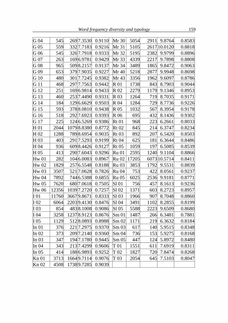
Word frequency diversity and typology

159

G 04 545 269 7.3530 0.9110 Mr 30 5054 2911 9.8764 0.8583 G 05 559 332 7.7183 0.9216 Mr 31 5105 2617 10.0120 0.8818 G 06 545 326 7.7918 0.9333 Mr 32 5195 2382 9.9799 0.8896 G 07 263 169 6.9781 0.9429 Mr 33 4339 2217 9.7898 0.8808 G 08 965 509 8.2157 0.9137 Mr 34 3489 1865 9.8472 0.9063 G 09 653 379 7.9035 0.9227 Mr 40 5218 2877 9.9948 0.8698 G 10 480 301 7.7245 0.9382 Mr 43 3356 1962 9.6097 0.8786 G 11 468 297 7.7563 0.9442 R 01 1738 843 8.7903 0.9044 G 12 251 169 6.9814 0.9433 R 02 2279 1179 9.1346 0.8953 G 13 460 253 7.4490 0.9331 R 03 1264 719 8.7035 0.9171 G 14 184 129 6.6629 0.9503 R 04 1284 729 8.7736 0.9226 G 15 593 378 8.0810 0.9438 R 05 1032 567 8.3954 0.9178 G 16 518 292 7.6923 0.9393 R 06 695 432 8.1436 0.9302 G 17 225 124 6.5269 0.9386 Rt 01 968 223 6.2661 0.8033 H 01 2044 1079 8.8380 0.8772 Rt 02 845 214 6.3747 0.8234 H 02 1288 789 8.6954 0.9035 Rt 03 892 207 6.5420 0.8503 H 03 403 291 7.5293 0.9199 Rt 04 625 181 6.3644 0.8486 H 04 936 609 8.4426 0.9127 Rt 05 1059 197 6.5085 0.8539 H 05 413 290 7.6043 0.9296 Ru 01 2595 1240 9.1104 0.8866 Hw 01 282 104 6.0083 0.8967 Ru 02 17205 6073 10.5714 0.8411 Hw 02 1829 257 6.5548 0.8188 Ru 03 3853 1792 9.5531 0.8839 Hw 03 3507 521 7.0628 0.7826 Ru 04 753 422 8.0561 0.9237 Hw 04 7892 744 6.5388 0.6855 Ru 05 6025 2536 9.9181 0.8771 Hw 05 7620 680 7.0618 0.7505 Sl 01 756 457 8.1613 0.9236 Hw 06 12356 1039 7.2720 0.7257 Sl 02 1371 603 8.2723 0.8957 I 01 11760 3667 9.8671 0.8333 Sl 03 1966 907 8.7048 0.8860 I 02 6064 2203 9.4130 0.8476 Sl 04 3491 1102 8.2855 0.8199 I 03 854 483 8.1008 0.9086 Sl 05 5588 2223 9.6509 0.8680 I 04 3258 1237 8.9123 0.8676 Sm 01 1487 266 6.3481 0.7881 I 05 1129 512 8.0893 0.8988 Sm 02 1171 219 6.3632 0.8184 In 01 376 221 7.2975 0.9370 Sm 03 617 140 5.9515 0.8348 In 02 373 209 7.2140 0.9360 Sm 04 736 153 5.9275 0.8168 In 03 347 194 7.1780 0.9445 Sm 05 447 124 5.8972 0.8480 In 04 343 213 7.4299 0.9606 T 01 1551 611 7.6919 0.8311 In 05 414 188 6.9893 0.9252 T 02 1827 720 7.8474 0.8268 Kn 01 3713 1664 9.7114 0.9076 T 03 2054 645 7.5103 0.8047 Kn 02 4508 1738 9.7285 0.9039

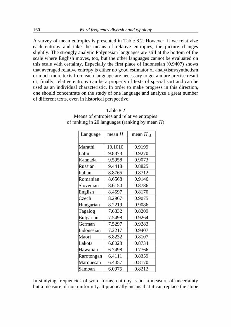
Word frequency diversity and typology

160

A survey of mean entropies is presented in Table 8.2. However, if we relativize each entropy and take the means of relative entropies, the picture changes slightly. The strongly analytic Polynesian languages are still at the bottom of the scale where English moves, too, but the other languages cannot be evaluated on this scale with certainty. Especially the first place of Indonesian (0.9407) shows that averaged relative entropy is either no good estimator of analytism/synthetism or much more texts from each language are necessary to get a more precise result or, finally, relative entropy can be a property of texts of special sort and can be used as an individual characteristic. In order to make progress in this direction, one should concentrate on the study of one language and analyze a great number of different texts, even in historical perspective.

Table 8.2 Means of entropies and relative entropies

of ranking in 20 languages (ranking by mean H)

Language mean H mean Hrel

Marathi 10.1010 0.9199 Latin 9.8373 0.9270 Kannada 9.5958 0.9073 Russian 9.4418 0.8825 Italian 8.8765 0.8712 Romanian 8.6568 0.9146 Slovenian 8.6150 0.8786 English 8.4597 0.8170 Czech 8.2967 0.9075 Hungarian 8.2219 0.9086 Tagalog 7.6832 0.8209 Bulgarian 7.5498 0.9264 German 7.5297 0.9283 Indonesian 7.2217 0.9407 Maori 6.8232 0.8107 Lakota 6.8028 0.8734 Hawaiian 6.7498 0.7766 Rarotongan 6.4111 0.8359 Marquesan 6.4057 0.8170 Samoan 6.0975 0.8212

In studying frequencies of word forms, entropy is not a measure of uncertainty but a measure of non uniformity. It practically means that it can replace the slope

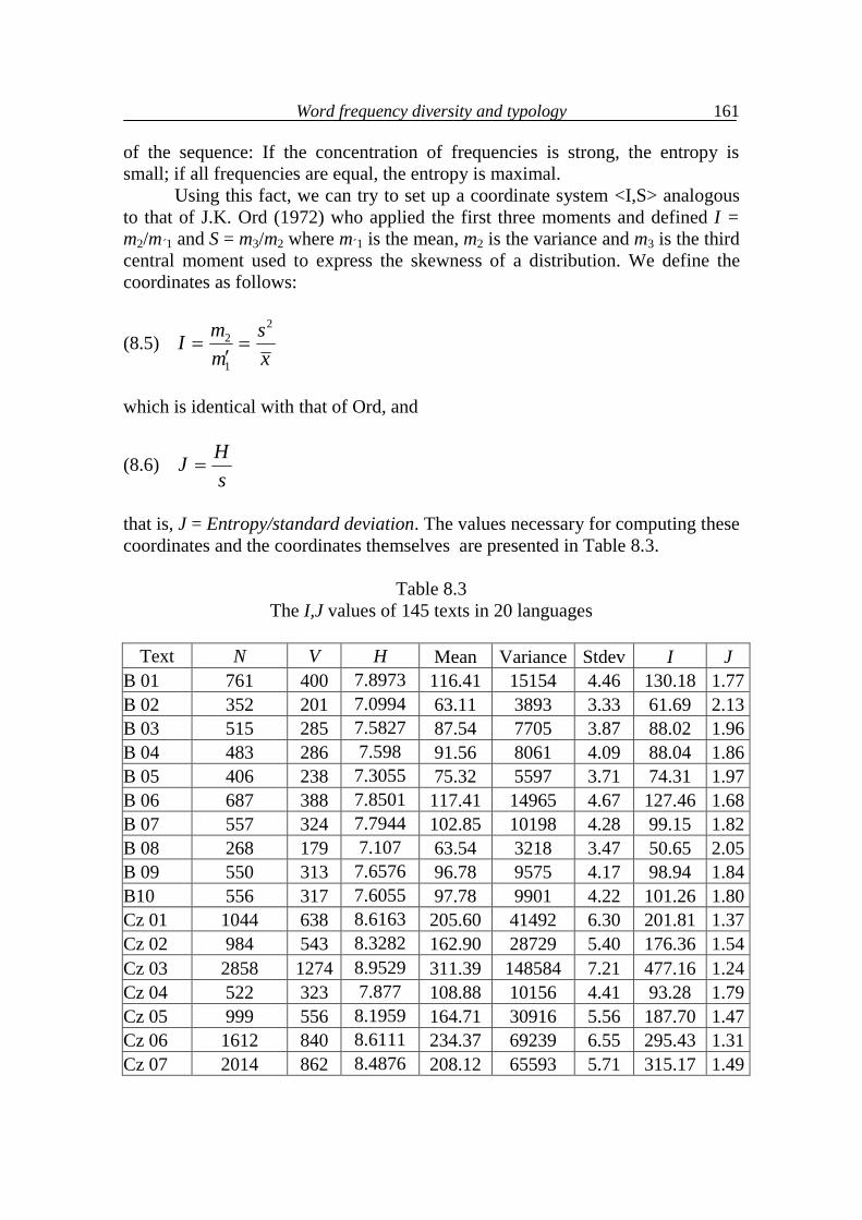
Word frequency diversity and typology

161

of the sequence: If the concentration of frequencies is strong, the entropy is small; if all frequencies are equal, the entropy is maximal. Using this fact, we can try to set up a coordinate system <I,S> analogous to that of J.K. Ord (1972) who applied the first three moments and defined I = m2/m´1 and S = m3/m2 where m´1 is the mean, m2 is the variance and m3 is the third central moment used to express the skewness of a distribution. We define the coordinates as follows:

(8.5) 2

2

1

m sIm x

which is identical with that of Ord, and

(8.6) HJs

that is, J = Entropy/standard deviation. The values necessary for computing these coordinates and the coordinates themselves are presented in Table 8.3.

Table 8.3 The I,J values of 145 texts in 20 languages

Text N V H Mean Variance Stdev I J

B 01 761 400 7.8973 116.41 15154 4.46 130.18 1.77 B 02 352 201 7.0994 63.11 3893 3.33 61.69 2.13 B 03 515 285 7.5827 87.54 7705 3.87 88.02 1.96 B 04 483 286 7.598 91.56 8061 4.09 88.04 1.86 B 05 406 238 7.3055 75.32 5597 3.71 74.31 1.97 B 06 687 388 7.8501 117.41 14965 4.67 127.46 1.68 B 07 557 324 7.7944 102.85 10198 4.28 99.15 1.82 B 08 268 179 7.107 63.54 3218 3.47 50.65 2.05 B 09 550 313 7.6576 96.78 9575 4.17 98.94 1.84 B10 556 317 7.6055 97.78 9901 4.22 101.26 1.80 Cz 01 1044 638 8.6163 205.60 41492 6.30 201.81 1.37 Cz 02 984 543 8.3282 162.90 28729 5.40 176.36 1.54 Cz 03 2858 1274 8.9529 311.39 148584 7.21 477.16 1.24 Cz 04 522 323 7.877 108.88 10156 4.41 93.28 1.79 Cz 05 999 556 8.1959 164.71 30916 5.56 187.70 1.47 Cz 06 1612 840 8.6111 234.37 69239 6.55 295.43 1.31 Cz 07 2014 862 8.4876 208.12 65593 5.71 315.17 1.49

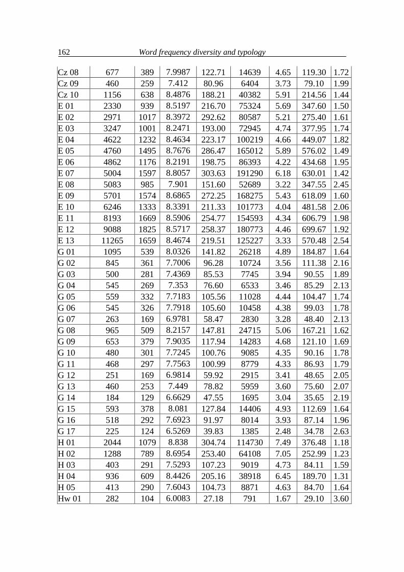
Word frequency diversity and typology

162

Cz 08 677 389 7.9987 122.71 14639 4.65 119.30 1.72 Cz 09 460 259 7.412 80.96 6404 3.73 79.10 1.99 Cz 10 1156 638 8.4876 188.21 40382 5.91 214.56 1.44 E 01 2330 939 8.5197 216.70 75324 5.69 347.60 1.50 E 02 2971 1017 8.3972 292.62 80587 5.21 275.40 1.61 E 03 3247 1001 8.2471 193.00 72945 4.74 377.95 1.74 E 04 4622 1232 8.4634 223.17 100219 4.66 449.07 1.82 E 05 4760 1495 8.7676 286.47 165012 5.89 576.02 1.49 E 06 4862 1176 8.2191 198.75 86393 4.22 434.68 1.95 E 07 5004 1597 8.8057 303.63 191290 6.18 630.01 1.42 E 08 5083 985 7.901 151.60 52689 3.22 347.55 2.45 E 09 5701 1574 8.6865 272.25 168275 5.43 618.09 1.60 E 10 6246 1333 8.3391 211.33 101773 4.04 481.58 2.06 E 11 8193 1669 8.5906 254.77 154593 4.34 606.79 1.98 E 12 9088 1825 8.5717 258.37 180773 4.46 699.67 1.92 E 13 11265 1659 8.4674 219.51 125227 3.33 570.48 2.54 G 01 1095 539 8.0326 141.82 26218 4.89 184.87 1.64 G 02 845 361 7.7006 96.28 10724 3.56 111.38 2.16 G 03 500 281 7.4369 85.53 7745 3.94 90.55 1.89 G 04 545 269 7.353 76.60 6533 3.46 85.29 2.13 G 05 559 332 7.7183 105.56 11028 4.44 104.47 1.74 G 06 545 326 7.7918 105.60 10458 4.38 99.03 1.78 G 07 263 169 6.9781 58.47 2830 3.28 48.40 2.13 G 08 965 509 8.2157 147.81 24715 5.06 167.21 1.62 G 09 653 379 7.9035 117.94 14283 4.68 121.10 1.69 G 10 480 301 7.7245 100.76 9085 4.35 90.16 1.78 G 11 468 297 7.7563 100.99 8779 4.33 86.93 1.79 G 12 251 169 6.9814 59.92 2915 3.41 48.65 2.05 G 13 460 253 7.449 78.82 5959 3.60 75.60 2.07 G 14 184 129 6.6629 47.55 1695 3.04 35.65 2.19 G 15 593 378 8.081 127.84 14406 4.93 112.69 1.64 G 16 518 292 7.6923 91.97 8014 3.93 87.14 1.96 G 17 225 124 6.5269 39.83 1385 2.48 34.78 2.63 H 01 2044 1079 8.838 304.74 114730 7.49 376.48 1.18 H 02 1288 789 8.6954 253.40 64108 7.05 252.99 1.23 H 03 403 291 7.5293 107.23 9019 4.73 84.11 1.59 H 04 936 609 8.4426 205.16 38918 6.45 189.70 1.31 H 05 413 290 7.6043 104.73 8871 4.63 84.70 1.64 Hw 01 282 104 6.0083 27.18 791 1.67 29.10 3.60

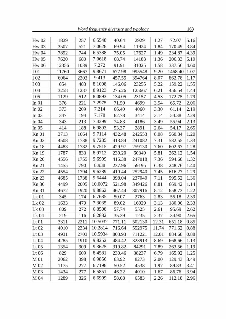
Word frequency diversity and typology

163

Hw 02 1829 257 6.5548 40.64 2929 1.27 72.07 5.16 Hw 03 3507 521 7.0628 69.94 11924 1.84 170.49 3.84 Hw 04 7892 744 6.5388 75.05 17627 1.49 234.87 4.39 Hw 05 7620 680 7.0618 68.74 14183 1.36 206.33 5.19 Hw 06 12356 1039 7.272 91.91 31025 1.58 337.56 4.60 I 01 11760 3667 9.8671 677.98 995548 9.20 1468.40 1.07 I 02 6064 2203 9.413 457.55 394764 8.07 862.78 1.17 I 03 854 483 8.1008 146.06 23255 5.22 159.22 1.55 I 04 3258 1237 8.9123 275.26 125667 6.21 456.54 1.44 I 05 1129 512 8.0893 134.05 23157 4.53 172.75 1.79 In 01 376 221 7.2975 71.50 4699 3.54 65.72 2.06 In 02 373 209 7.214 66.40 4060 3.30 61.14 2.19 In 03 347 194 7.178 62.78 3414 3.14 54.38 2.29 In 04 343 213 7.4299 74.83 4186 3.49 55.94 2.13 In 05 414 188 6.9893 53.37 2891 2.64 54.17 2.65 Kn 01 3713 1664 9.7114 432.48 242553 8.08 560.84 1.20 Kn 02 4508 1738 9.7285 413.84 241082 7.31 582.55 1.33 Kn 18 4483 1782 9.7515 429.97 259130 7.60 602.67 1.28 Kn 19 1787 833 8.9712 230.20 60340 5.81 262.12 1.54 Kn 20 4556 1755 9.6909 415.38 247018 7.36 594.68 1.32 Kn 21 1455 790 8.938 237.96 59195 6.38 248.76 1.40 Kn 22 4554 1794 9.6289 410.44 252940 7.45 616.27 1.29 Kn 23 4685 1738 9.6444 398.04 237040 7.11 595.52 1.36 Kn 30 4499 2005 10.0072 521.98 349426 8.81 669.42 1.14 Kn 31 4672 1920 9.8862 467.44 307916 8.12 658.73 1.22 Lk 01 345 174 6.7685 50.07 2763 2.83 55.18 2.39 Lk 02 1633 479 7.3035 89.02 16029 3.13 180.06 2.33 Lk 03 809 272 6.8508 57.74 5525 2.61 95.69 2.62 Lk 04 219 116 6.2882 35.39 1235 2.37 34.90 2.65 Lt 01 3311 2211 10.5032 771.11 502130 12.31 651.18 0.85 Lt 02 4010 2334 10.2814 716.64 552975 11.74 771.62 0.88 Lt 03 4931 2703 10.5934 803.93 711221 12.01 884.68 0.88 Lt 04 4285 1910 9.8252 484.42 323913 8.69 668.66 1.13 Lt 05 1354 909 9.3625 319.82 84291 7.89 263.56 1.19 Lt 06 829 609 8.4581 230.46 38237 6.79 165.92 1.25 M 01 2062 398 6.9856 63.92 8273 2.00 129.43 3.49 M 02 1175 277 6.7198 50.52 4538 1.97 89.83 3.41 M 03 1434 277 6.5851 46.22 4010 1.67 86.76 3.94 M 04 1289 326 6.6909 58.68 6583 2.26 112.18 2.96

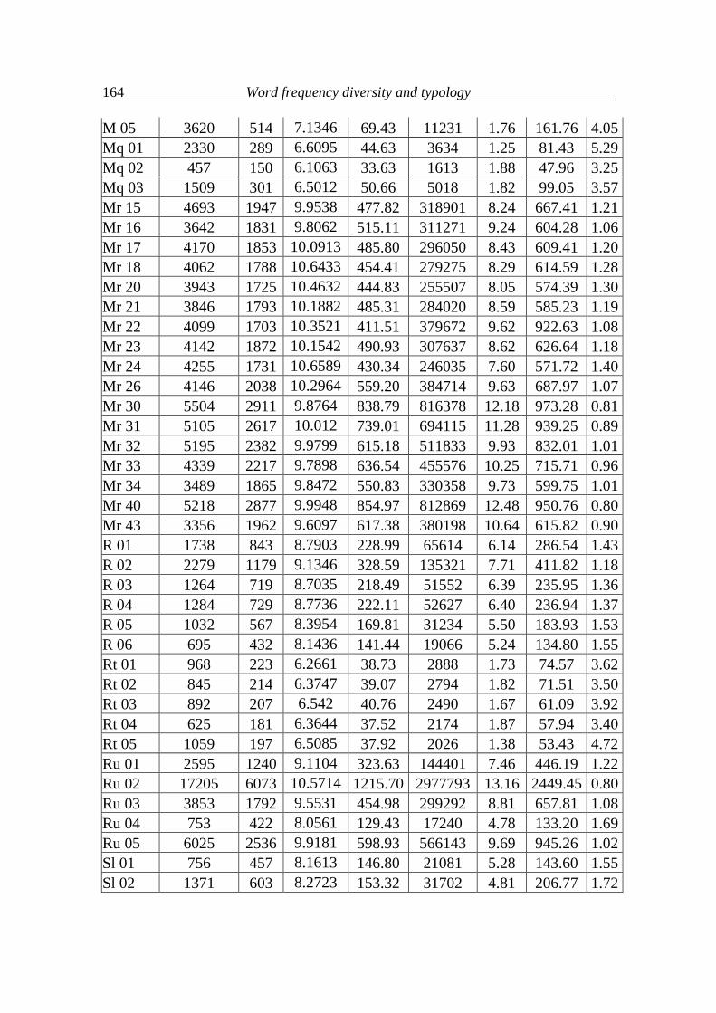
Word frequency diversity and typology

164

M 05 3620 514 7.1346 69.43 11231 1.76 161.76 4.05 Mq 01 2330 289 6.6095 44.63 3634 1.25 81.43 5.29 Mq 02 457 150 6.1063 33.63 1613 1.88 47.96 3.25 Mq 03 1509 301 6.5012 50.66 5018 1.82 99.05 3.57 Mr 15 4693 1947 9.9538 477.82 318901 8.24 667.41 1.21 Mr 16 3642 1831 9.8062 515.11 311271 9.24 604.28 1.06 Mr 17 4170 1853 10.0913 485.80 296050 8.43 609.41 1.20 Mr 18 4062 1788 10.6433 454.41 279275 8.29 614.59 1.28 Mr 20 3943 1725 10.4632 444.83 255507 8.05 574.39 1.30 Mr 21 3846 1793 10.1882 485.31 284020 8.59 585.23 1.19 Mr 22 4099 1703 10.3521 411.51 379672 9.62 922.63 1.08 Mr 23 4142 1872 10.1542 490.93 307637 8.62 626.64 1.18 Mr 24 4255 1731 10.6589 430.34 246035 7.60 571.72 1.40 Mr 26 4146 2038 10.2964 559.20 384714 9.63 687.97 1.07 Mr 30 5504 2911 9.8764 838.79 816378 12.18 973.28 0.81 Mr 31 5105 2617 10.012 739.01 694115 11.28 939.25 0.89 Mr 32 5195 2382 9.9799 615.18 511833 9.93 832.01 1.01 Mr 33 4339 2217 9.7898 636.54 455576 10.25 715.71 0.96 Mr 34 3489 1865 9.8472 550.83 330358 9.73 599.75 1.01 Mr 40 5218 2877 9.9948 854.97 812869 12.48 950.76 0.80 Mr 43 3356 1962 9.6097 617.38 380198 10.64 615.82 0.90 R 01 1738 843 8.7903 228.99 65614 6.14 286.54 1.43 R 02 2279 1179 9.1346 328.59 135321 7.71 411.82 1.18 R 03 1264 719 8.7035 218.49 51552 6.39 235.95 1.36 R 04 1284 729 8.7736 222.11 52627 6.40 236.94 1.37 R 05 1032 567 8.3954 169.81 31234 5.50 183.93 1.53 R 06 695 432 8.1436 141.44 19066 5.24 134.80 1.55 Rt 01 968 223 6.2661 38.73 2888 1.73 74.57 3.62 Rt 02 845 214 6.3747 39.07 2794 1.82 71.51 3.50 Rt 03 892 207 6.542 40.76 2490 1.67 61.09 3.92 Rt 04 625 181 6.3644 37.52 2174 1.87 57.94 3.40 Rt 05 1059 197 6.5085 37.92 2026 1.38 53.43 4.72 Ru 01 2595 1240 9.1104 323.63 144401 7.46 446.19 1.22 Ru 02 17205 6073 10.5714 1215.70 2977793 13.16 2449.45 0.80 Ru 03 3853 1792 9.5531 454.98 299292 8.81 657.81 1.08 Ru 04 753 422 8.0561 129.43 17240 4.78 133.20 1.69 Ru 05 6025 2536 9.9181 598.93 566143 9.69 945.26 1.02 Sl 01 756 457 8.1613 146.80 21081 5.28 143.60 1.55 Sl 02 1371 603 8.2723 153.32 31702 4.81 206.77 1.72

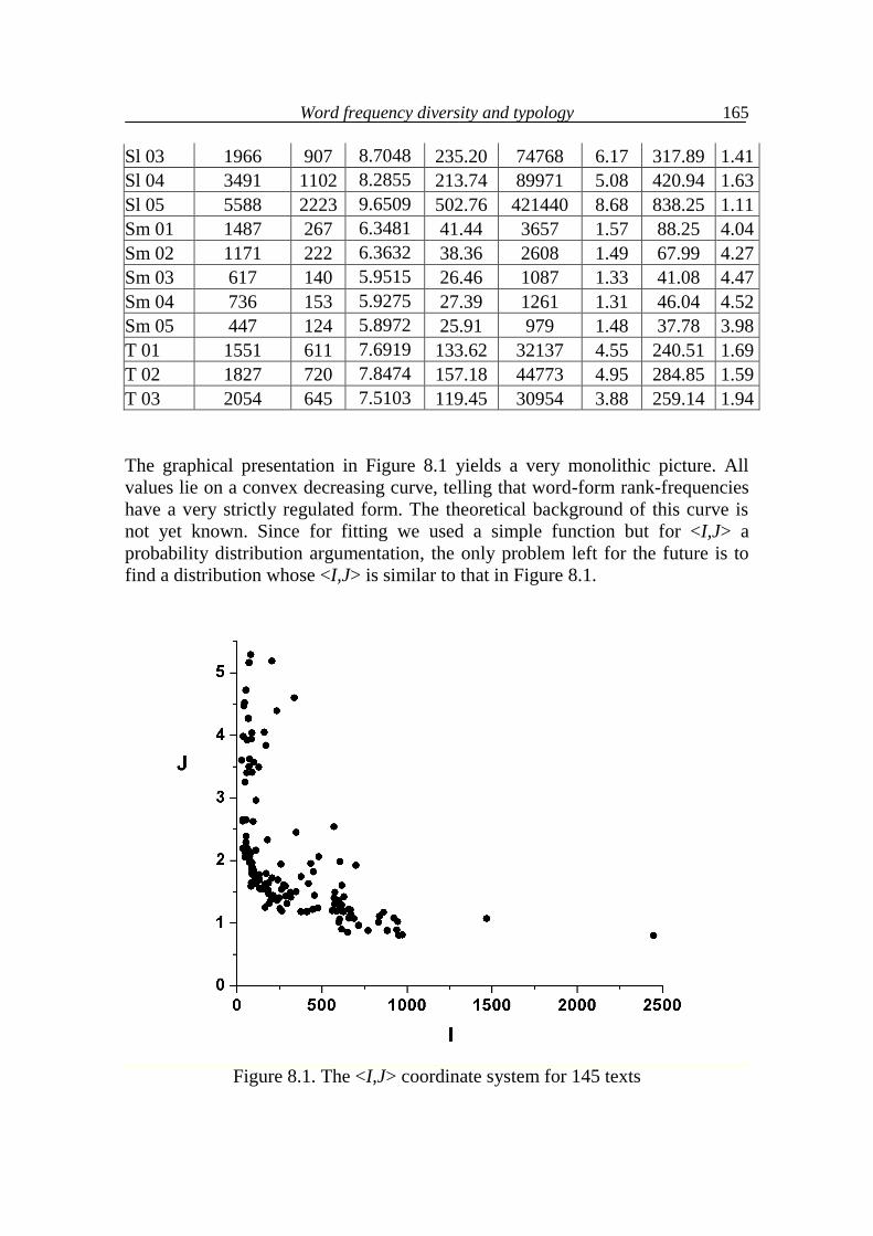
Word frequency diversity and typology

165

Sl 03 1966 907 8.7048 235.20 74768 6.17 317.89 1.41 Sl 04 3491 1102 8.2855 213.74 89971 5.08 420.94 1.63 Sl 05 5588 2223 9.6509 502.76 421440 8.68 838.25 1.11 Sm 01 1487 267 6.3481 41.44 3657 1.57 88.25 4.04 Sm 02 1171 222 6.3632 38.36 2608 1.49 67.99 4.27 Sm 03 617 140 5.9515 26.46 1087 1.33 41.08 4.47 Sm 04 736 153 5.9275 27.39 1261 1.31 46.04 4.52 Sm 05 447 124 5.8972 25.91 979 1.48 37.78 3.98 T 01 1551 611 7.6919 133.62 32137 4.55 240.51 1.69 T 02 1827 720 7.8474 157.18 44773 4.95 284.85 1.59 T 03 2054 645 7.5103 119.45 30954 3.88 259.14 1.94 The graphical presentation in Figure 8.1 yields a very monolithic picture. All values lie on a convex decreasing curve, telling that word-form rank-frequencies have a very strictly regulated form. The theoretical background of this curve is not yet known. Since for fitting we used a simple function but for <I,J> a probability distribution argumentation, the only problem left for the future is to find a distribution whose <I,J> is similar to that in Figure 8.1.

Figure 8.1. The <I,J> coordinate system for 145 texts

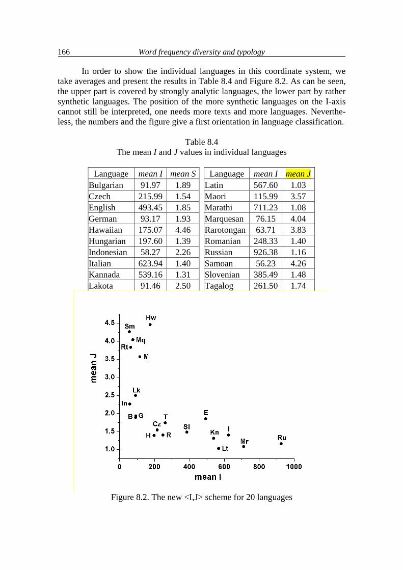
Word frequency diversity and typology

166

In order to show the individual languages in this coordinate system, we take averages and present the results in Table 8.4 and Figure 8.2. As can be seen, the upper part is covered by strongly analytic languages, the lower part by rather synthetic languages. The position of the more synthetic languages on the I-axis cannot still be interpreted, one needs more texts and more languages. Neverthe-less, the numbers and the figure give a first orientation in language classification.

Table 8.4 The mean I and J values in individual languages

Language mean I mean S Language mean I mean J

Bulgarian 91.97 1.89 Latin 567.60 1.03 Czech 215.99 1.54 Maori 115.99 3.57 English 493.45 1.85 Marathi 711.23 1.08 German 93.17 1.93 Marquesan 76.15 4.04 Hawaiian 175.07 4.46 Rarotongan 63.71 3.83 Hungarian 197.60 1.39 Romanian 248.33 1.40 Indonesian 58.27 2.26 Russian 926.38 1.16 Italian 623.94 1.40 Samoan 56.23 4.26 Kannada 539.16 1.31 Slovenian 385.49 1.48 Lakota 91.46 2.50 Tagalog 261.50 1.74

Figure 8.2. The new <I,J> scheme for 20 languages

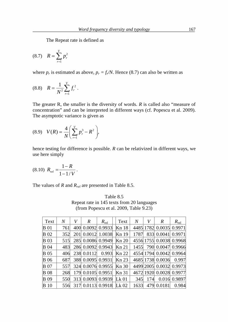
Word frequency diversity and typology

167

The Repeat rate is defined as

(8.7) 2

1

V

rr

R p

where pr is estimated as above, pr = fr/N. Hence (8.7) can also be written as

(8.8) 22

1

1 V

rr

R fN

.

The greater R, the smaller is the diversity of words. R is called also “measure of concentration” and can be interpreted in different ways (cf. Popescu et al. 2009). The asymptotic variance is given as

(8.9) 3 2

1

4( )V

rr

V R p RN

,

hence testing for difference is possible. R can be relativized in different ways, we use here simply

(8.10) 1

1 1 /relRRV

.

The values of R and Rrel are presented in Table 8.5.

Table 8.5 Repeat rate in 145 texts from 20 languages

(from Popescu et al. 2009, Table 9.23)

Text N V R Rrel Text N V R Rrel B 01 761 400 0.0092 0.9933 Kn 18 4485 1782 0.0035 0.9971 B 02 352 201 0.0012 1.0038 Kn 19 1787 833 0.0041 0.9971 B 03 515 285 0.0086 0.9949 Kn 20 4556 1755 0.0038 0.9968 B 04 483 286 0.0092 0.9943 Kn 21 1455 790 0.0047 0.9966 B 05 406 238 0.0112 0.993 Kn 22 4554 1794 0.0042 0.9964 B 06 687 388 0.0095 0.9931 Kn 23 4685 1738 0.0036 0.997 B 07 557 324 0.0076 0.9955 Kn 30 4499 2005 0.0032 0.9973 B 08 268 179 0.0105 0.9951 Kn 31 4672 1920 0.0028 0.9977 B 09 550 313 0.0093 0.9939 Lk 01 345 174 0.016 0.9897 B 10 556 317 0.0113 0.9918 Lk 02 1633 479 0.0181 0.984

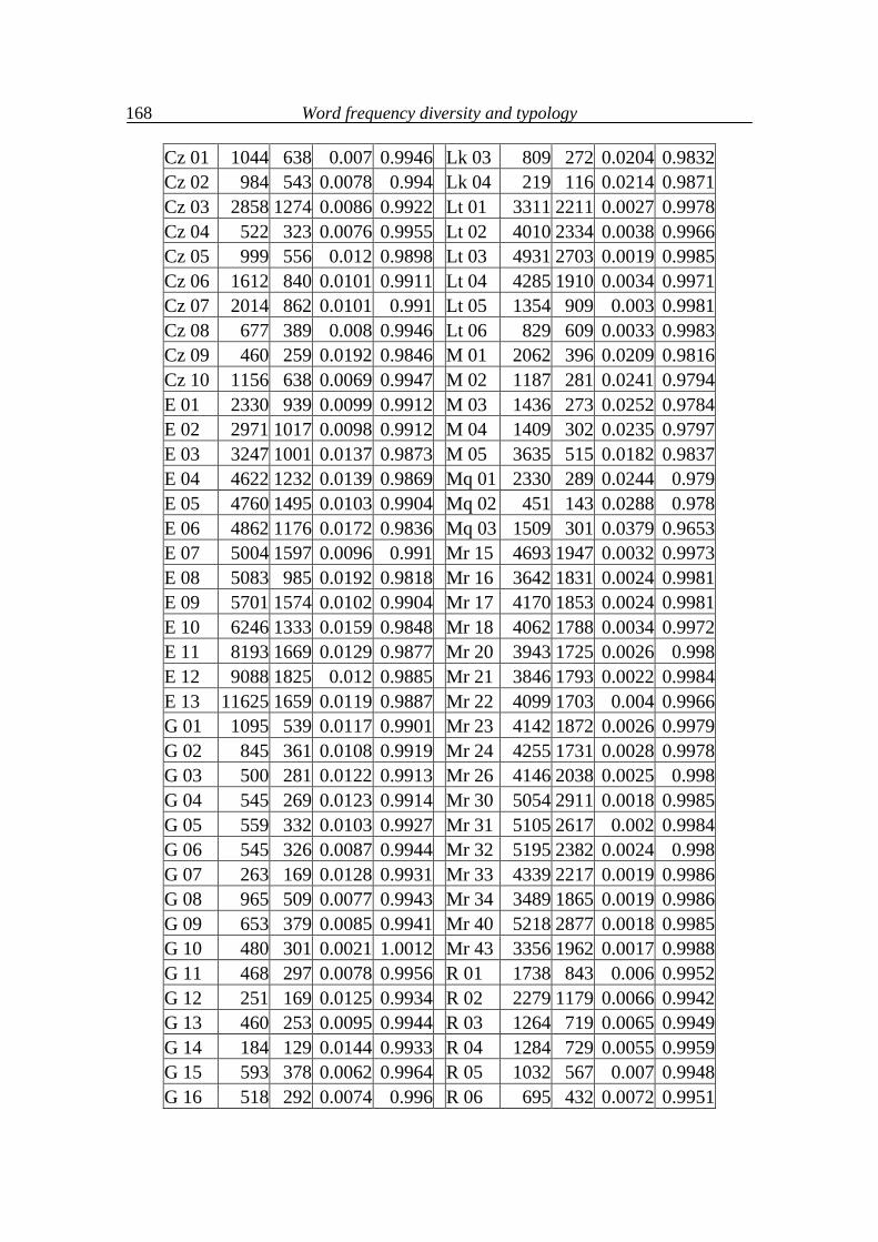
Word frequency diversity and typology

168

Cz 01 1044 638 0.007 0.9946 Lk 03 809 272 0.0204 0.9832 Cz 02 984 543 0.0078 0.994 Lk 04 219 116 0.0214 0.9871 Cz 03 2858 1274 0.0086 0.9922 Lt 01 3311 2211 0.0027 0.9978 Cz 04 522 323 0.0076 0.9955 Lt 02 4010 2334 0.0038 0.9966 Cz 05 999 556 0.012 0.9898 Lt 03 4931 2703 0.0019 0.9985 Cz 06 1612 840 0.0101 0.9911 Lt 04 4285 1910 0.0034 0.9971 Cz 07 2014 862 0.0101 0.991 Lt 05 1354 909 0.003 0.9981 Cz 08 677 389 0.008 0.9946 Lt 06 829 609 0.0033 0.9983 Cz 09 460 259 0.0192 0.9846 M 01 2062 396 0.0209 0.9816 Cz 10 1156 638 0.0069 0.9947 M 02 1187 281 0.0241 0.9794 E 01 2330 939 0.0099 0.9912 M 03 1436 273 0.0252 0.9784 E 02 2971 1017 0.0098 0.9912 M 04 1409 302 0.0235 0.9797 E 03 3247 1001 0.0137 0.9873 M 05 3635 515 0.0182 0.9837 E 04 4622 1232 0.0139 0.9869 Mq 01 2330 289 0.0244 0.979 E 05 4760 1495 0.0103 0.9904 Mq 02 451 143 0.0288 0.978 E 06 4862 1176 0.0172 0.9836 Mq 03 1509 301 0.0379 0.9653 E 07 5004 1597 0.0096 0.991 Mr 15 4693 1947 0.0032 0.9973 E 08 5083 985 0.0192 0.9818 Mr 16 3642 1831 0.0024 0.9981 E 09 5701 1574 0.0102 0.9904 Mr 17 4170 1853 0.0024 0.9981 E 10 6246 1333 0.0159 0.9848 Mr 18 4062 1788 0.0034 0.9972 E 11 8193 1669 0.0129 0.9877 Mr 20 3943 1725 0.0026 0.998 E 12 9088 1825 0.012 0.9885 Mr 21 3846 1793 0.0022 0.9984 E 13 11625 1659 0.0119 0.9887 Mr 22 4099 1703 0.004 0.9966 G 01 1095 539 0.0117 0.9901 Mr 23 4142 1872 0.0026 0.9979 G 02 845 361 0.0108 0.9919 Mr 24 4255 1731 0.0028 0.9978 G 03 500 281 0.0122 0.9913 Mr 26 4146 2038 0.0025 0.998 G 04 545 269 0.0123 0.9914 Mr 30 5054 2911 0.0018 0.9985 G 05 559 332 0.0103 0.9927 Mr 31 5105 2617 0.002 0.9984 G 06 545 326 0.0087 0.9944 Mr 32 5195 2382 0.0024 0.998 G 07 263 169 0.0128 0.9931 Mr 33 4339 2217 0.0019 0.9986 G 08 965 509 0.0077 0.9943 Mr 34 3489 1865 0.0019 0.9986 G 09 653 379 0.0085 0.9941 Mr 40 5218 2877 0.0018 0.9985 G 10 480 301 0.0021 1.0012 Mr 43 3356 1962 0.0017 0.9988 G 11 468 297 0.0078 0.9956 R 01 1738 843 0.006 0.9952 G 12 251 169 0.0125 0.9934 R 02 2279 1179 0.0066 0.9942 G 13 460 253 0.0095 0.9944 R 03 1264 719 0.0065 0.9949 G 14 184 129 0.0144 0.9933 R 04 1284 729 0.0055 0.9959 G 15 593 378 0.0062 0.9964 R 05 1032 567 0.007 0.9948 G 16 518 292 0.0074 0.996 R 06 695 432 0.0072 0.9951

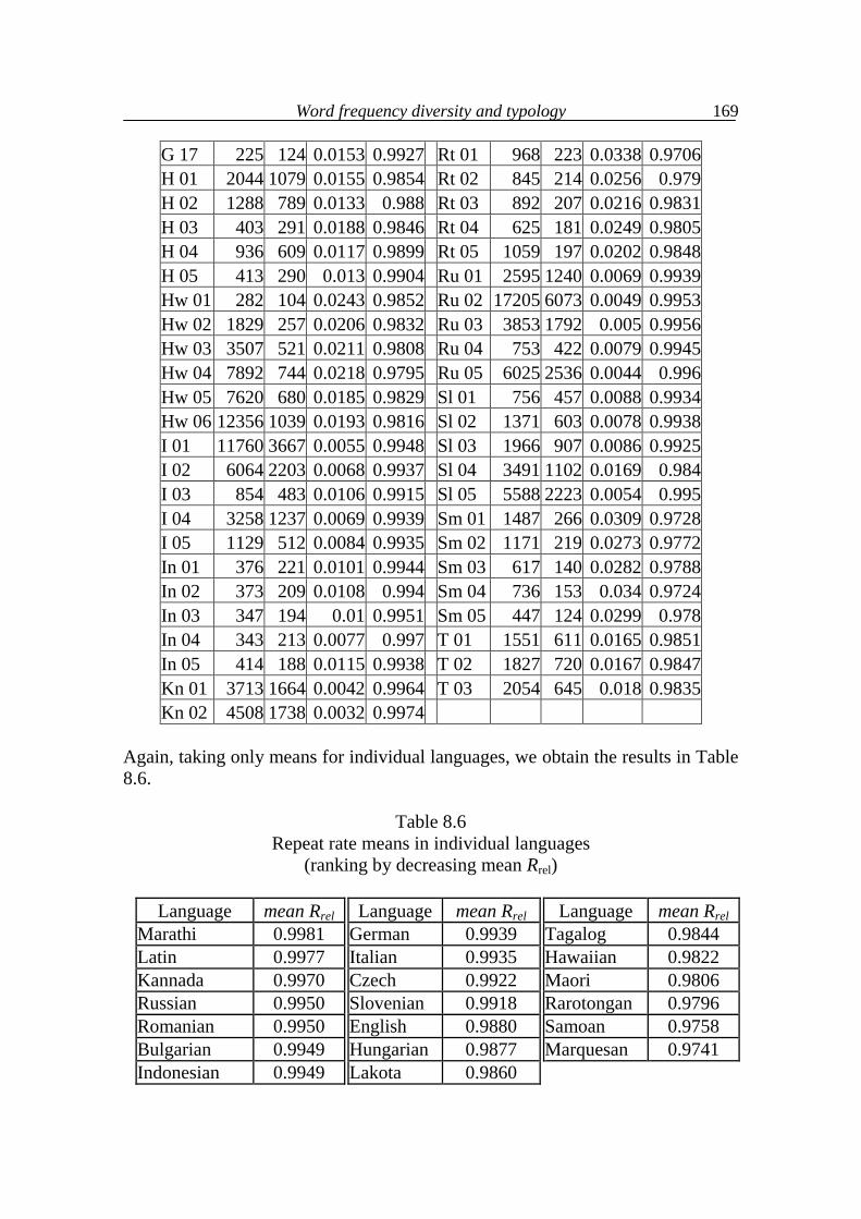
Word frequency diversity and typology

169

G 17 225 124 0.0153 0.9927 Rt 01 968 223 0.0338 0.9706 H 01 2044 1079 0.0155 0.9854 Rt 02 845 214 0.0256 0.979 H 02 1288 789 0.0133 0.988 Rt 03 892 207 0.0216 0.9831 H 03 403 291 0.0188 0.9846 Rt 04 625 181 0.0249 0.9805 H 04 936 609 0.0117 0.9899 Rt 05 1059 197 0.0202 0.9848 H 05 413 290 0.013 0.9904 Ru 01 2595 1240 0.0069 0.9939 Hw 01 282 104 0.0243 0.9852 Ru 02 17205 6073 0.0049 0.9953 Hw 02 1829 257 0.0206 0.9832 Ru 03 3853 1792 0.005 0.9956 Hw 03 3507 521 0.0211 0.9808 Ru 04 753 422 0.0079 0.9945 Hw 04 7892 744 0.0218 0.9795 Ru 05 6025 2536 0.0044 0.996 Hw 05 7620 680 0.0185 0.9829 Sl 01 756 457 0.0088 0.9934 Hw 06 12356 1039 0.0193 0.9816 Sl 02 1371 603 0.0078 0.9938 I 01 11760 3667 0.0055 0.9948 Sl 03 1966 907 0.0086 0.9925 I 02 6064 2203 0.0068 0.9937 Sl 04 3491 1102 0.0169 0.984 I 03 854 483 0.0106 0.9915 Sl 05 5588 2223 0.0054 0.995 I 04 3258 1237 0.0069 0.9939 Sm 01 1487 266 0.0309 0.9728 I 05 1129 512 0.0084 0.9935 Sm 02 1171 219 0.0273 0.9772 In 01 376 221 0.0101 0.9944 Sm 03 617 140 0.0282 0.9788 In 02 373 209 0.0108 0.994 Sm 04 736 153 0.034 0.9724 In 03 347 194 0.01 0.9951 Sm 05 447 124 0.0299 0.978 In 04 343 213 0.0077 0.997 T 01 1551 611 0.0165 0.9851 In 05 414 188 0.0115 0.9938 T 02 1827 720 0.0167 0.9847 Kn 01 3713 1664 0.0042 0.9964 T 03 2054 645 0.018 0.9835 Kn 02 4508 1738 0.0032 0.9974

Again, taking only means for individual languages, we obtain the results in Table 8.6.

Table 8.6 Repeat rate means in individual languages

(ranking by decreasing mean Rrel)

Language mean Rrel Language mean Rrel Language mean Rrel Marathi 0.9981 German 0.9939 Tagalog 0.9844 Latin 0.9977 Italian 0.9935 Hawaiian 0.9822 Kannada 0.9970 Czech 0.9922 Maori 0.9806 Russian 0.9950 Slovenian 0.9918 Rarotongan 0.9796 Romanian 0.9950 English 0.9880 Samoan 0.9758 Bulgarian 0.9949 Hungarian 0.9877 Marquesan 0.9741 Indonesian 0.9949 Lakota 0.9860

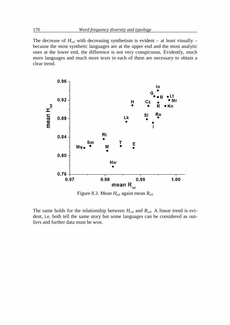
Word frequency diversity and typology

170

The decrease of Hrel with decreasing synthetism is evident – at least visually – because the most synthetic languages are at the upper end and the most analytic ones at the lower end, the difference is not very conspicuous. Evidently, much more languages and much more texts in each of them are necessary to obtain a clear trend.

Figure 8.3. Mean Hrel agaist mean Rrel

The same holds for the relationship between Hrel and Rrel. A linear trend is evi-dent, i.e. both tell the same story but some languages can be considered as out-liers and further data must be won.

9. Nominal style

The concept of “nominal style“ designates a view from a special standpoint not necessarily adequate for every language. It is an attempt to characterize a text ac-cording to the weight of nouns in it. Different other “styles” are e.g. ornamental style taking into account the weight of adjectives, or active style taking into account that of verbs designating activity, etc. Usually, a special class of words is opposed to another class and their proportions are compared. Style is a kind of property and as such it is a matter of degree. However, the concept of “nominal style” (or any other style) can be oper-ationalized in many ways. It need not be simply the proportion of nouns in a text because in that case the given proportion should be compared with that in the population, but there are no populations in language (cf. Orlov, Boroda, Nada-rejšvili 1982). It may be the comparison of the number of nouns and verbs in a text, as is usually made in German where nominal expressions are very fre-quently used in official language (e.g. verbannen vs. in Verbannung schicken; beweisen vs. unter Beweis stellen). It does not mean that a verb is replaced by a noun but that a noun is added. In this way the proportion of nouns in the text increases. If a language clearly distinguishes between nouns and verb, it is al-ways possible to choose one of the above ways: taking the relative frequency of nouns in the given text or comparing their absolute frequency with that of some other word class. And since style is a choice among possibilities, properties of this type are characteristic of text, style, author, genre, etc. but not of language. A similar definition concerning active vs. descriptive style has been devised as early as in 1925 by A. Busemann. The above situation can be captured either statically, counting the given words and weighting or comparing them, or dynamically, counting the position (time) of appearance of given words in text. 9.1. Static approach One usually characterizes the situation using an indicator with the following properties: (a) It is simple, (b) it can be interpreted philologically, (c) it has a defined range, (d) it allows easy testing, i.e., its distribution or only some sampling properties are known. Let us begin with a very simple indicator

(9.1) 1 SIS V

,

Nominal style

172

where S is the number of nouns and V that of verbs in a text. It is a simple pro-portion between <0,1>, S is distributed binomially, the variance is Var(I1) = I1(1 - I1)/(S + V) and its interpretation is as follows: if I1 ≈ 0.5, then there is an equilibrium, i.e. to each noun there is a verb; if I1 > 0.5 significantly, then the text begins to be nominal, i.e. either many Vs are replaced by V+S, or verbal phrases contain additional nouns etc.; if I1 < 0.5 significantly, then the “verbality” grows, the nouns obtain more active predicates, the text gets more “active”. If the same indicator is defined using verbs and adjectives, one obtains a measure of descriptivity/activity (cf. Busemann 1925; Altmann 1978). Of course, the definition and the operationalization of the indicator depend on the aim of the analysis and on including or excluding copula, auxiliary verbs or modal verbs, too, etc. Consider, e.g., the first strophe of Goethe´s “Erlkönig” in which there are 5 V (including all verbs) and 6 S. The above indicator yields I1 = 6/(6+5) = 0.5455, i.e. there is an approximate nominal-verbal equilibrium and the result can be used for characterization. However, automatically the question arises how many nouns must accompany 5 verbs in order to consider the style significantly nominal. The problem can be solved very simply because the situation is binomial. Let S + V = n and E(I1) = p = 0.5 under the H0 hypothesis of equi-librium. Our hypothesis H1: p > 0.5, i.e. we ask what is the probability of finding S or more nouns. To this end one computes

(9.2) ( ) 0.5n

n

x S

nP X S

x

.

the cumulative probability of the binomial distribution b(n,p). In our case with S = 6, V = 5, n = 11 we obtain P(X ≥ 6) = 0.5 which is a sign of equilibrium. If we set S = 7, V = 5, n = 12, we obtain P = 0.3872, etc. With S = 13, V = 5, n = 18 we obtain P = 0.048, a number which is smaller than 0.05, the usual significance level. Thus the above text is rather in equilibrium than being nominal. Though I1 can be used always for characterization, the test for significance can be performed also without computing the cumulative prob-ability of the binomial distribution which gets tiresome if n is great. Another sim-ple possibility is using the chi-square criterion yielding an approximate result. Let the expected number of S and V be n/2 under the H0 hypothesis, i.e., in equilibrium there is the same number of S and of V. Then the chi-square criterion for divergence is (ignoring all other classes of words)

Nominal style

173

(9.3)

2 2

2( ) ( )

2 2

2 2

n nS VX n n

.

Reordering the formula and replacing n = S+V we obtain

(9.4) 2

2 ( )S VXS V

,

representing the chi-square with 1 degree of freedom. A more complex deriva-tion using the likelihood ratio can be found in Altmann (1978, 1988: 23-29). Consider again the above example using S = 13, V = 5, then X2 = (13-5)2/(13+5) = 3.5556. The probability of this chi-square is 0.0593, slightly above the 0.05 level (which is at 3.64) being a good approximation to the binomial probability. The chi-square test is two-sided. Since the root of chi-square with 1 degree of freedom is a normal variable, the root of (9.4) can be written in the form

(9.5) 2 1Su nn

representing a normal variable. Inserting the values S = 13, n = 18, we obtain u = [2(13)/18-1]√18 = 1.8856 which is exactly the root of X2. The associated probability of u for a two-sided test is 0.0594, i.e. identical with that of the chi-square, slightly greater than the binomial probability which is exact. For the complete “Erlkönig” with S = 53, V = 41 we obtain P = 0.1282, X2 = 1.53, u = 1.24, i.e. a nominal-verbal equilibrium. Now, if we only measure the extent of nominality, (9.1) is sufficient. But if we speak about significant nominality or verbality we can make our decisions in the following way:

(a) If S > V and P(X ≥ S) ≤ 0.05 or X2 ≥ 3.64 or u ≥ 1.96, we consider the style as nominal;

(b) if S < V and P(X ≤ S) ≤ 0.05 or X2 ≥ 3.64 or u ≤ -1.96, we consider the style as verbal;

(c) in all the other cases we speak about nominal-verbal equilibrium. Needless to say, the chi-square has its weak points when the S and V are either too small or too large. If one is interested in text classification, one can set up

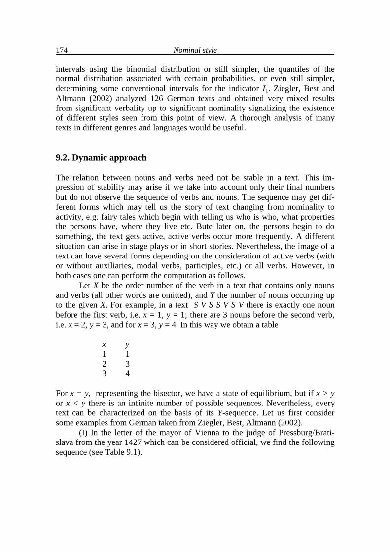
Nominal style

174

intervals using the binomial distribution or still simpler, the quantiles of the normal distribution associated with certain probabilities, or even still simpler, determining some conventional intervals for the indicator I1. Ziegler, Best and Altmann (2002) analyzed 126 German texts and obtained very mixed results from significant verbality up to significant nominality signalizing the existence of different styles seen from this point of view. A thorough analysis of many texts in different genres and languages would be useful. 9.2. Dynamic approach The relation between nouns and verbs need not be stable in a text. This im-pression of stability may arise if we take into account only their final numbers but do not observe the sequence of verbs and nouns. The sequence may get dif-ferent forms which may tell us the story of text changing from nominality to activity, e.g. fairy tales which begin with telling us who is who, what properties the persons have, where they live etc. Bute later on, the persons begin to do something, the text gets active, active verbs occur more frequently. A different situation can arise in stage plays or in short stories. Nevertheless, the image of a text can have several forms depending on the consideration of active verbs (with or without auxiliaries, modal verbs, participles, etc.) or all verbs. However, in both cases one can perform the computation as follows. Let X be the order number of the verb in a text that contains only nouns and verbs (all other words are omitted), and Y the number of nouns occurring up to the given X. For example, in a text S V S S V S V there is exactly one noun before the first verb, i.e. x = 1, y = 1; there are 3 nouns before the second verb, i.e. x = 2, y = 3, and for x = 3, y = 4. In this way we obtain a table x y 1 1 2 3 3 4 For x = y, representing the bisector, we have a state of equilibrium, but if x > y or x < y there is an infinite number of possible sequences. Nevertheless, every text can be characterized on the basis of its Y-sequence. Let us first consider some examples from German taken from Ziegler, Best, Altmann (2002). (I) In the letter of the mayor of Vienna to the judge of Pressburg/Brati-slava from the year 1427 which can be considered official, we find the following sequence (see Table 9.1).

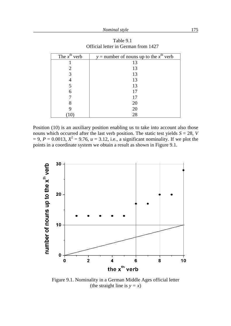
Nominal style

175

Table 9.1 Official letter in German from 1427

Position (10) is an auxiliary position enabling us to take into account also those nouns which occurred after the last verb position. The static test yields S = 28, V = 9, P = 0.0013, X2 = 9.76, u = 3.12, i.e., a significant nominality. If we plot the points in a coordinate system we obtain a result as shown in Figure 9.1.

Figure 9.1. Nominality in a German Middle Ages official letter

(the straight line is y = x)

The xth verb y = number of nouns up to the xth verb 1 2 3 4 5 6 7 8 9

(10)

13 13 13 13 13 17 17 20 20 28

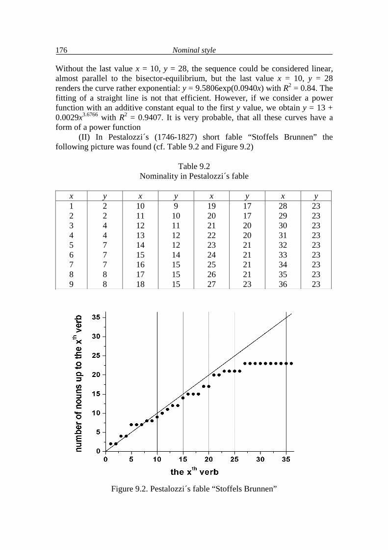
Nominal style

176

Without the last value x = 10, y = 28, the sequence could be considered linear, almost parallel to the bisector-equilibrium, but the last value x = 10, y = 28 renders the curve rather exponential: y = 9.5806exp(0.0940x) with R2 = 0.84. The fitting of a straight line is not that efficient. However, if we consider a power function with an additive constant equal to the first y value, we obtain y = 13 + 0.0029x3.6766 with R2 = 0.9407. It is very probable, that all these curves have a form of a power function (II) In Pestalozzi´s (1746-1827) short fable “Stoffels Brunnen” the following picture was found (cf. Table 9.2 and Figure 9.2)

Table 9.2 Nominality in Pestalozzi´s fable

x y x y x y x y 1 2 3 4 5 6 7 8 9

2 2 4 4 7 7 7 8 8

10 11 12 13 14 15 16 17 18

9 10 11 12 12 14 15 15 15

19 20 21 22 23 24 25 26 27

17 17 20 20 21 21 21 21 23

28 29 30 31 32 33 34 35 36

23 23 23 23 23 23 23 23 23

Figure 9.2. Pestalozzi´s fable “Stoffels Brunnen”

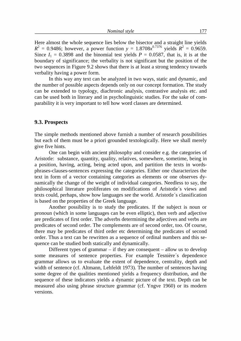
Nominal style

177

Here almost the whole sequence lies below the bisector and a straight line yields R2 = 0.9486; however, a power function y = 1.8708x0.7376 yields R2 = 0.9659. Since I1 = 0.3898 and the binomial test yields P = 0.0587, that is, it is at the boundary of significance; the verbality is not significant but the position of the two sequences in Figure 9.2 shows that there is at least a strong tendency towards verbality having a power form. In this way any text can be analyzed in two ways, static and dynamic, and the number of possible aspects depends only on our concept formation. The study can be extended to typology, diachronic analysis, contrastive analysis etc. and can be used both in literary and in psycholinguistic studies. For the sake of com-parability it is very important to tell how word classes are determined. 9.3. Prospects The simple methods mentioned above furnish a number of research possibilities but each of them must be a priori grounded textologically. Here we shall merely give five hints. One can begin with ancient philosophy and consider e.g. the categories of Aristotle: substance, quantity, quality, relatives, somewhere, sometime, being in a position, having, acting, being acted upon, and partition the texts in words-phrases-clauses-sentences expressing the categories. Either one characterizes the text in form of a vector containing categories as elements or one observes dy-namically the change of the weight of individual categories. Needless to say, the philosophical literature proliferates on modifications of Aristotle´s views and texts could, perhaps, show how languages see the world. Aristotle´s classification is based on the properties of the Greek language. Another possibility is to study the predicates. If the subject is noun or pronoun (which in some languages can be even elliptic), then verb and adjective are predicates of first order. The adverbs determining the adjectives and verbs are predicates of second order. The complements are of second order, too. Of course, there may be predicates of third order etc determining the predicates of second order. Thus a text can be rewritten as a sequence of ordinal numbers and this se-quence can be studied both statically and dynamically. Different types of grammar – if they are consequent – allow us to develop some measures of sentence properties. For example Tesnière´s dependence grammar allows us to evaluate the extent of dependence, centrality, depth and width of sentence (cf. Altmann, Lehfeldt 1973). The number of sentences having some degree of the qualities mentioned yields a frequency distribution, and the sequence of these indicators yields a dynamic picture of the text. Depth can be measured also using phrase structure grammar (cf. Yngve 1960) or its modern versions.

Nominal style

178

A stage play is a sequence of speech acts which can be either classified or quantified from a special point of view. It is to be expected that a comedy will have a different sequence of speech acts than a drama. Classical dramas have a very specific profile but comedies do not. Hence, the frequencies of speech acts and their sequences again yield a kind of text structure which can be captured quantitatively. In psycholinguistics and language teaching, a number of different measures of text difficulty, dogmatism etc. have been developed. They have been used to characterize texts, persons etc. but usually testing or modeling the dynamics were omitted. All this and many other vistas are possible and each of them would fill a book.

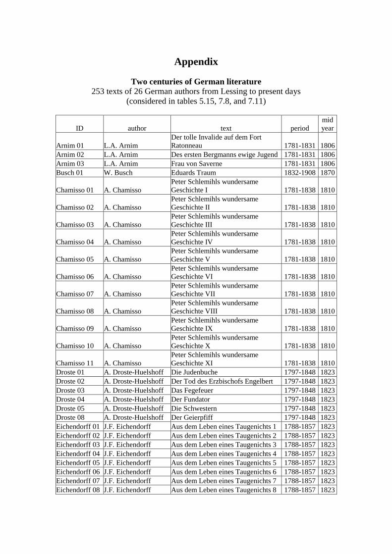
Appendix

Two centuries of German literature 253 texts of 26 German authors from Lessing to present days

(considered in tables 5.15, 7.8, and 7.11)

ID author text period mid year

Arnim 01 L.A. Arnim Der tolle Invalide auf dem Fort Ratonneau 1781-1831 1806

Arnim 02 L.A. Arnim Des ersten Bergmanns ewige Jugend 1781-1831 1806 Arnim 03 L.A. Arnim Frau von Saverne 1781-1831 1806 Busch 01 W. Busch Eduards Traum 1832-1908 1870

Chamisso 01 A. Chamisso Peter Schlemihls wundersame Geschichte I 1781-1838 1810

Chamisso 02 A. Chamisso Peter Schlemihls wundersame Geschichte II 1781-1838 1810

Chamisso 03 A. Chamisso Peter Schlemihls wundersame Geschichte III 1781-1838 1810

Chamisso 04 A. Chamisso Peter Schlemihls wundersame Geschichte IV 1781-1838 1810

Chamisso 05 A. Chamisso Peter Schlemihls wundersame Geschichte V 1781-1838 1810

Chamisso 06 A. Chamisso Peter Schlemihls wundersame Geschichte VI 1781-1838 1810

Chamisso 07 A. Chamisso Peter Schlemihls wundersame Geschichte VII 1781-1838 1810

Chamisso 08 A. Chamisso Peter Schlemihls wundersame Geschichte VIII 1781-1838 1810

Chamisso 09 A. Chamisso Peter Schlemihls wundersame Geschichte IX 1781-1838 1810

Chamisso 10 A. Chamisso Peter Schlemihls wundersame Geschichte X 1781-1838 1810

Chamisso 11 A. Chamisso Peter Schlemihls wundersame Geschichte XI 1781-1838 1810

Droste 01 A. Droste-Huelshoff Die Judenbuche 1797-1848 1823 Droste 02 A. Droste-Huelshoff Der Tod des Erzbischofs Engelbert 1797-1848 1823 Droste 03 A. Droste-Huelshoff Das Fegefeuer 1797-1848 1823 Droste 04 A. Droste-Huelshoff Der Fundator 1797-1848 1823 Droste 05 A. Droste-Huelshoff Die Schwestern 1797-1848 1823 Droste 08 A. Droste-Huelshoff Der Geierpfiff 1797-1848 1823 Eichendorff 01 J.F. Eichendorff Aus dem Leben eines Taugenichts 1 1788-1857 1823 Eichendorff 02 J.F. Eichendorff Aus dem Leben eines Taugenichts 2 1788-1857 1823 Eichendorff 03 J.F. Eichendorff Aus dem Leben eines Taugenichts 3 1788-1857 1823 Eichendorff 04 J.F. Eichendorff Aus dem Leben eines Taugenichts 4 1788-1857 1823 Eichendorff 05 J.F. Eichendorff Aus dem Leben eines Taugenichts 5 1788-1857 1823 Eichendorff 06 J.F. Eichendorff Aus dem Leben eines Taugenichts 6 1788-1857 1823 Eichendorff 07 J.F. Eichendorff Aus dem Leben eines Taugenichts 7 1788-1857 1823 Eichendorff 08 J.F. Eichendorff Aus dem Leben eines Taugenichts 8 1788-1857 1823

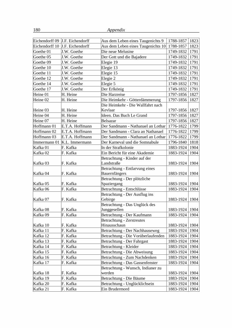
Appendix

180

Eichendorff 09 J.F. Eichendorff Aus dem Leben eines Taugenichts 9 1788-1857 1823 Eichendorff 10 J.F. Eichendorff Aus dem Leben eines Taugenichts 10 1788-1857 1823 Goethe 01 J.W. Goethe Die neue Melusine 1749-1832 1791 Goethe 05 J.W. Goethe Der Gott und die Bajadere 1749-1832 1791 Goethe 09 J.W. Goethe Elegie 19 1749-1832 1791 Goethe 10 J.W. Goethe Elegie 13 1749-1832 1791 Goethe 11 J.W. Goethe Elegie 15 1749-1832 1791 Goethe 12 J.W. Goethe Elegie 2 1749-1832 1791 Goethe 14 J.W. Goethe Elegie 5 1749-1832 1791 Goethe 17 J.W. Goethe Der Erlkönig 1749-1832 1791 Heine 01 H. Heine Die Harzreise 1797-1856 1827 Heine 02 H. Heine Die Heimkehr - Götterdämmerung 1797-1856 1827

Heine 03 H. Heine Die Heimkehr - Die Wallfahrt nach Kevlaar 1797-1856 1827

Heine 04 H. Heine Ideen. Das Buch Le Grand 1797-1856 1827 Heine 07 H. Heine Belsazar 1797-1856 1827 Hoffmann 01 E.T.A. Hoffmann Der Sandmann - Nathanael an Lothar 1776-1822 1799 Hoffmann 02 E.T.A. Hoffmann Der Sandmann - Clara an Nathanael 1776-1822 1799 Hoffmann 03 E.T.A. Hoffmann Der Sandmann - Nathanael an Lothar 1776-1822 1799 Immermann 01 K.L. Immermann Der Karneval und die Somnabule 1796-1840 1818 Kafka 01 F. Kafka In der Strafkolonie 1883-1924 1904 Kafka 02 F. Kafka Ein Bericht für eine Akademie 1883-1924 1904

Kafka 03 F. Kafka Betrachtung - Kinder auf der Landstraße 1883-1924 1904

Kafka 04 F. Kafka Betrachtung - Entlarvung eines Bauernfängers 1883-1924 1904

Kafka 05 F. Kafka Betrachtung - Der plötzliche Spaziergang 1883-1924 1904

Kafka 06 F. Kafka Betrachtung - Entschlüsse 1883-1924 1904

Kafka 07 F. Kafka Betrachtung - Der Ausflug ins Gebirge 1883-1924 1904

Kafka 08 F. Kafka Betrachtung - Das Unglück des Junggesellen 1883-1924 1904

Kafka 09 F. Kafka Betrachtung - Der Kaufmann 1883-1924 1904

Kafka 10 F. Kafka Betrachtung - Zerstreutes Hinausschaun 1883-1924 1904

Kafka 11 F. Kafka Betrachtung - Der Nachhauseweg 1883-1924 1904 Kafka 12 F. Kafka Betrachtung - Die Vorüberlaufenden 1883-1924 1904 Kafka 13 F. Kafka Betrachtung - Der Fahrgast 1883-1924 1904 Kafka 14 F. Kafka Betrachtung - Kleider 1883-1924 1904 Kafka 15 F. Kafka Betrachtung - Die Abweisung 1883-1924 1904 Kafka 16 F. Kafka Betrachtung - Zum Nachdenken 1883-1924 1904 Kafka 17 F. Kafka Betrachtung - Das Gassenfenster 1883-1924 1904

Kafka 18 F. Kafka Betrachtung - Wunsch, Indianer zu werden 1883-1924 1904

Kafka 19 F. Kafka Betrachtung - Die Bäume 1883-1924 1904 Kafka 20 F. Kafka Betrachtung - Unglücklichsein 1883-1924 1904 Kafka 21 F. Kafka Ein Brudermord 1883-1924 1904

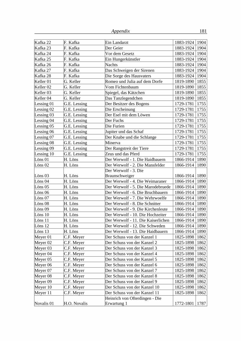
Appendix

181

Kafka 22 F. Kafka Ein Landarzt 1883-1924 1904 Kafka 23 F. Kafka Der Geier 1883-1924 1904 Kafka 24 F. Kafka Vor dem Gesetz 1883-1924 1904 Kafka 25 F. Kafka Ein Hungerkünstler 1883-1924 1904 Kafka 26 F. Kafka Nachts 1883-1924 1904 Kafka 27 F. Kafka Das Schweigen der Sirenen 1883-1924 1904 Kafka 28 F. Kafka Die Sorge des Hausvaters 1883-1924 1904 Keller 01 G. Keller Romeo und Julia auf dem Dorfe 1819-1890 1855 Keller 02 G. Keller Vom Fichtenbaum 1819-1890 1855 Keller 03 G. Keller Spiegel, das Kätzchen 1819-1890 1855 Keller 04 G. Keller Das Tanzlegendchen 1819-1890 1855 Lessing 01 G.E. Lessing Der Besitzer des Bogens 1729-1781 1755 Lessing 02 G.E. Lessing Die Erscheinung 1729-1781 1755 Lessing 03 G.E. Lessing Der Esel mit dem Löwen 1729-1781 1755 Lessing 04 G.E. Lessing Der Fuchs 1729-1781 1755 Lessing 05 G.E. Lessing Die Furien 1729-1781 1755 Lessing 06 G.E. Lessing Jupiter und das Schaf 1729-1781 1755 Lessing 07 G.E. Lessing Der Knabe und die Schlange 1729-1781 1755 Lessing 08 G.E. Lessing Minerva 1729-1781 1755 Lessing 09 G.E. Lessing Der Rangstreit der Tiere 1729-1781 1755 Lessing 10 G.E. Lessing Zeus und das Pferd 1729-1781 1755 Löns 01 H. Löns Der Werwolf - 1. Die Haidbauern 1866-1914 1890 Löns 02 H. Löns Der Werwolf - 2. Die Mansfelder 1866-1914 1890

Löns 03 H. Löns Der Werwolf - 3. Die Braunschweiger 1866-1914 1890

Löns 04 H. Löns Der Werwolf - 4. Die Weimaraner 1866-1914 1890 Löns 05 H. Löns Der Werwolf - 5. Die Marodebruede 1866-1914 1890 Löns 06 H. Löns Der Werwolf - 6. Die Bruchbauern 1866-1914 1890 Löns 07 H. Löns Der Werwolf - 7. Die Wehrwoelfe 1866-1914 1890 Löns 08 H. Löns Der Werwolf - 8. Die Schnitter 1866-1914 1890 Löns 09 H. Löns Der Werwolf - 9. Die Kirchenleute 1866-1914 1890 Löns 10 H. Löns Der Werwolf - 10. Die Hochzeiter 1866-1914 1890 Löns 11 H. Löns Der Werwolf - 11. Die Kaiserlichen 1866-1914 1890 Löns 12 H. Löns Der Werwolf - 12. Die Schweden 1866-1914 1890 Löns 13 H. Löns Der Werwolf - 13. Die Haidbauern 1866-1914 1890 Meyer 01 C.F. Meyer Der Schuss von der Kanzel 1 1825-1898 1862 Meyer 02 C.F. Meyer Der Schuss von der Kanzel 2 1825-1898 1862 Meyer 03 C.F. Meyer Der Schuss von der Kanzel 3 1825-1898 1862 Meyer 04 C.F. Meyer Der Schuss von der Kanzel 4 1825-1898 1862 Meyer 05 C.F. Meyer Der Schuss von der Kanzel 5 1825-1898 1862 Meyer 06 C.F. Meyer Der Schuss von der Kanzel 6 1825-1898 1862 Meyer 07 C.F. Meyer Der Schuss von der Kanzel 7 1825-1898 1862 Meyer 08 C.F. Meyer Der Schuss von der Kanzel 8 1825-1898 1862 Meyer 09 C.F. Meyer Der Schuss von der Kanzel 9 1825-1898 1862 Meyer 10 C.F. Meyer Der Schuss von der Kanzel 10 1825-1898 1862 Meyer 11 C.F. Meyer Der Schuss von der Kanzel 11 1825-1898 1862

Novalis 01 H.O. Novalis Heinrich von Ofterdingen - Die Erwartung 1 1772-1801 1787

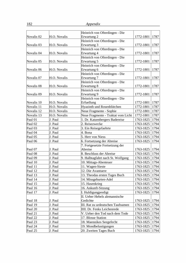
Appendix

182

Novalis 02 H.O. Novalis Heinrich von Ofterdingen - Die Erwartung 2 1772-1801 1787

Novalis 03 H.O. Novalis Heinrich von Ofterdingen - Die Erwartung 3 1772-1801 1787

Novalis 04 H.O. Novalis Heinrich von Ofterdingen - Die Erwartung 4 1772-1801 1787

Novalis 05 H.O. Novalis Heinrich von Ofterdingen - Die Erwartung 5 1772-1801 1787

Novalis 06 H.O. Novalis Heinrich von Ofterdingen - Die Erwartung 6 1772-1801 1787

Novalis 07 H.O. Novalis Heinrich von Ofterdingen - Die Erwartung 7 1772-1801 1787

Novalis 08 H.O. Novalis Heinrich von Ofterdingen - Die Erwartung 8 1772-1801 1787

Novalis 09 H.O. Novalis Heinrich von Ofterdingen - Die Erwartung 9 1772-1801 1787

Novalis 10 H.O. Novalis Heinrich von Ofterdingen - Die Erfuellung 1772-1801 1787

Novalis 11 H.O. Novalis Hyazinth und Rosenblütchen 1772-1801 1787 Novalis 12 H.O. Novalis Neue Fragmente - Sophie 1772-1801 1787 Novalis 13 H.O. Novalis Neue Fragmente - Traktat vom Licht 1772-1801 1787 Paul 01 J. Paul 1. Dr. Katzenbergers Badereise 1763-1825 1794 Paul 02 J. Paul 2. Reisezwecke 1763-1825 1794 Paul 03 J. Paul 3. Ein Reisegefaehrte 1763-1825 1794 Paul 04 J. Paul 4. Bona 1763-1825 1794 Paul 05 J. Paul 5. Herr von Niess 1763-1825 1794 Paul 06 J. Paul 6. Fortsetzung der Abreise 1763-1825 1794

Paul 07 J. Paul 7. Fortgesetzte Fortsetzung der Abreise 1763-1825 1794

Paul 08 J. Paul 8. Beschluss der Abreise 1763-1825 1794 Paul 09 J. Paul 9. Halbtagfahrt nach St. Wolfgang 1763-1825 1794 Paul 10 J. Paul 10. Mittags-Abenteuer 1763-1825 1794 Paul 11 J. Paul 11. Wagen-Sieste 1763-1825 1794 Paul 12 J. Paul 12. Die Avantuere 1763-1825 1794 Paul 13 J. Paul 13. Theodas ersten Tages Buch 1763-1825 1794 Paul 14 J. Paul 14. Missgeburten-Adel 1763-1825 1794 Paul 15 J. Paul 15. Hasenkrieg 1763-1825 1794 Paul 16 J. Paul 16. Ankunft-Sitzung 1763-1825 1794 Paul 17 J. Paul I. Huldigungpredigt 1763-1825 1794

Paul 18 J. Paul II. Ueber Hebels alemannische Gedichte 1763-1825 1794

Paul 19 J. Paul III. Rat zu urdeutschen Taufnamen 1763-1825 1794 Paul 20 J. Paul IIII. Dr. Fenks Leichenrede 1763-1825 1794 Paul 21 J. Paul V. Ueber den Tod nach dem Tode 1763-1825 1794 Paul 22 J. Paul 17. Blosse Station 1763-1825 1794 Paul 23 J. Paul 18. Maennikes Seegefecht 1763-1825 1794 Paul 24 J. Paul 19. Mondbelustigungen 1763-1825 1794 Paul 25 J. Paul 20. Zweiten Tages Buch 1763-1825 1794

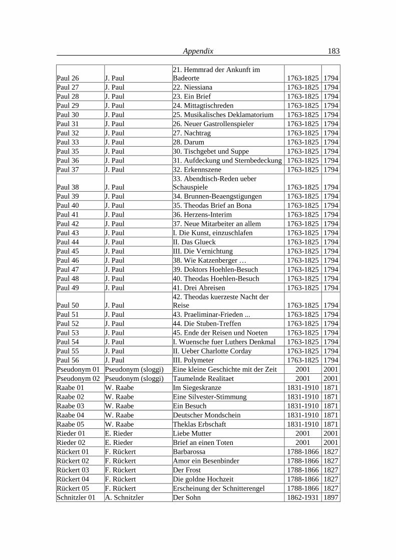
Appendix

183

Paul 26 J. Paul 21. Hemmrad der Ankunft im Badeorte 1763-1825 1794

Paul 27 J. Paul 22. Niessiana 1763-1825 1794 Paul 28 J. Paul 23. Ein Brief 1763-1825 1794 Paul 29 J. Paul 24. Mittagtischreden 1763-1825 1794 Paul 30 J. Paul 25. Musikalisches Deklamatorium 1763-1825 1794 Paul 31 J. Paul 26. Neuer Gastrollenspieler 1763-1825 1794 Paul 32 J. Paul 27. Nachtrag 1763-1825 1794 Paul 33 J. Paul 28. Darum 1763-1825 1794 Paul 35 J. Paul 30. Tischgebet und Suppe 1763-1825 1794 Paul 36 J. Paul 31. Aufdeckung und Sternbedeckung 1763-1825 1794 Paul 37 J. Paul 32. Erkennszene 1763-1825 1794

Paul 38 J. Paul 33. Abendtisch-Reden ueber Schauspiele 1763-1825 1794

Paul 39 J. Paul 34. Brunnen-Beaengstigungen 1763-1825 1794 Paul 40 J. Paul 35. Theodas Brief an Bona 1763-1825 1794 Paul 41 J. Paul 36. Herzens-Interim 1763-1825 1794 Paul 42 J. Paul 37. Neue Mitarbeiter an allem 1763-1825 1794 Paul 43 J. Paul I. Die Kunst, einzuschlafen 1763-1825 1794 Paul 44 J. Paul II. Das Glueck 1763-1825 1794 Paul 45 J. Paul III. Die Vernichtung 1763-1825 1794 Paul 46 J. Paul 38. Wie Katzenberger … 1763-1825 1794 Paul 47 J. Paul 39. Doktors Hoehlen-Besuch 1763-1825 1794 Paul 48 J. Paul 40. Theodas Hoehlen-Besuch 1763-1825 1794 Paul 49 J. Paul 41. Drei Abreisen 1763-1825 1794

Paul 50 J. Paul 42. Theodas kuerzeste Nacht der Reise 1763-1825 1794

Paul 51 J. Paul 43. Praeliminar-Frieden ... 1763-1825 1794 Paul 52 J. Paul 44. Die Stuben-Treffen 1763-1825 1794 Paul 53 J. Paul 45. Ende der Reisen und Noeten 1763-1825 1794 Paul 54 J. Paul I. Wuensche fuer Luthers Denkmal 1763-1825 1794 Paul 55 J. Paul II. Ueber Charlotte Corday 1763-1825 1794 Paul 56 J. Paul III. Polymeter 1763-1825 1794 Pseudonym 01 Pseudonym (sloggi) Eine kleine Geschichte mit der Zeit 2001 2001 Pseudonym 02 Pseudonym (sloggi) Taumelnde Realitaet 2001 2001 Raabe 01 W. Raabe Im Siegeskranze 1831-1910 1871 Raabe 02 W. Raabe Eine Silvester-Stimmung 1831-1910 1871 Raabe 03 W. Raabe Ein Besuch 1831-1910 1871 Raabe 04 W. Raabe Deutscher Mondschein 1831-1910 1871 Raabe 05 W. Raabe Theklas Erbschaft 1831-1910 1871 Rieder 01 E. Rieder Liebe Mutter 2001 2001 Rieder 02 E. Rieder Brief an einen Toten 2001 2001 Rückert 01 F. Rückert Barbarossa 1788-1866 1827 Rückert 02 F. Rückert Amor ein Besenbinder 1788-1866 1827 Rückert 03 F. Rückert Der Frost 1788-1866 1827 Rückert 04 F. Rückert Die goldne Hochzeit 1788-1866 1827 Rückert 05 F. Rückert Erscheinung der Schnitterengel 1788-1866 1827 Schnitzler 01 A. Schnitzler Der Sohn 1862-1931 1897

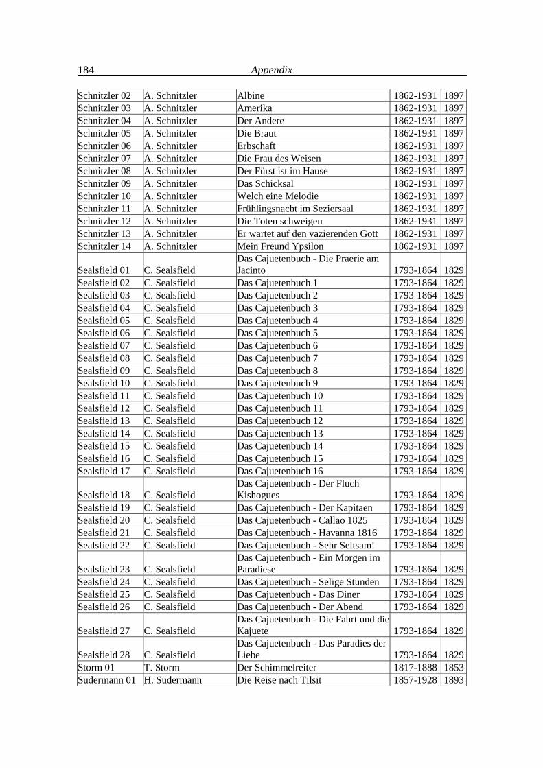
Appendix

184

Schnitzler 02 A. Schnitzler Albine 1862-1931 1897 Schnitzler 03 A. Schnitzler Amerika 1862-1931 1897 Schnitzler 04 A. Schnitzler Der Andere 1862-1931 1897 Schnitzler 05 A. Schnitzler Die Braut 1862-1931 1897 Schnitzler 06 A. Schnitzler Erbschaft 1862-1931 1897 Schnitzler 07 A. Schnitzler Die Frau des Weisen 1862-1931 1897 Schnitzler 08 A. Schnitzler Der Fürst ist im Hause 1862-1931 1897 Schnitzler 09 A. Schnitzler Das Schicksal 1862-1931 1897 Schnitzler 10 A. Schnitzler Welch eine Melodie 1862-1931 1897 Schnitzler 11 A. Schnitzler Frühlingsnacht im Seziersaal 1862-1931 1897 Schnitzler 12 A. Schnitzler Die Toten schweigen 1862-1931 1897 Schnitzler 13 A. Schnitzler Er wartet auf den vazierenden Gott 1862-1931 1897 Schnitzler 14 A. Schnitzler Mein Freund Ypsilon 1862-1931 1897

Sealsfield 01 C. Sealsfield Das Cajuetenbuch - Die Praerie am Jacinto 1793-1864 1829

Sealsfield 02 C. Sealsfield Das Cajuetenbuch 1 1793-1864 1829 Sealsfield 03 C. Sealsfield Das Cajuetenbuch 2 1793-1864 1829 Sealsfield 04 C. Sealsfield Das Cajuetenbuch 3 1793-1864 1829 Sealsfield 05 C. Sealsfield Das Cajuetenbuch 4 1793-1864 1829 Sealsfield 06 C. Sealsfield Das Cajuetenbuch 5 1793-1864 1829 Sealsfield 07 C. Sealsfield Das Cajuetenbuch 6 1793-1864 1829 Sealsfield 08 C. Sealsfield Das Cajuetenbuch 7 1793-1864 1829 Sealsfield 09 C. Sealsfield Das Cajuetenbuch 8 1793-1864 1829 Sealsfield 10 C. Sealsfield Das Cajuetenbuch 9 1793-1864 1829 Sealsfield 11 C. Sealsfield Das Cajuetenbuch 10 1793-1864 1829 Sealsfield 12 C. Sealsfield Das Cajuetenbuch 11 1793-1864 1829 Sealsfield 13 C. Sealsfield Das Cajuetenbuch 12 1793-1864 1829 Sealsfield 14 C. Sealsfield Das Cajuetenbuch 13 1793-1864 1829 Sealsfield 15 C. Sealsfield Das Cajuetenbuch 14 1793-1864 1829 Sealsfield 16 C. Sealsfield Das Cajuetenbuch 15 1793-1864 1829 Sealsfield 17 C. Sealsfield Das Cajuetenbuch 16 1793-1864 1829

Sealsfield 18 C. Sealsfield Das Cajuetenbuch - Der Fluch Kishogues 1793-1864 1829

Sealsfield 19 C. Sealsfield Das Cajuetenbuch - Der Kapitaen 1793-1864 1829 Sealsfield 20 C. Sealsfield Das Cajuetenbuch - Callao 1825 1793-1864 1829 Sealsfield 21 C. Sealsfield Das Cajuetenbuch - Havanna 1816 1793-1864 1829 Sealsfield 22 C. Sealsfield Das Cajuetenbuch - Sehr Seltsam! 1793-1864 1829

Sealsfield 23 C. Sealsfield Das Cajuetenbuch - Ein Morgen im Paradiese 1793-1864 1829

Sealsfield 24 C. Sealsfield Das Cajuetenbuch - Selige Stunden 1793-1864 1829 Sealsfield 25 C. Sealsfield Das Cajuetenbuch - Das Diner 1793-1864 1829 Sealsfield 26 C. Sealsfield Das Cajuetenbuch - Der Abend 1793-1864 1829

Sealsfield 27 C. Sealsfield Das Cajuetenbuch - Die Fahrt und die Kajuete 1793-1864 1829

Sealsfield 28 C. Sealsfield Das Cajuetenbuch - Das Paradies der Liebe 1793-1864 1829

Storm 01 T. Storm Der Schimmelreiter 1817-1888 1853 Sudermann 01 H. Sudermann Die Reise nach Tilsit 1857-1928 1893

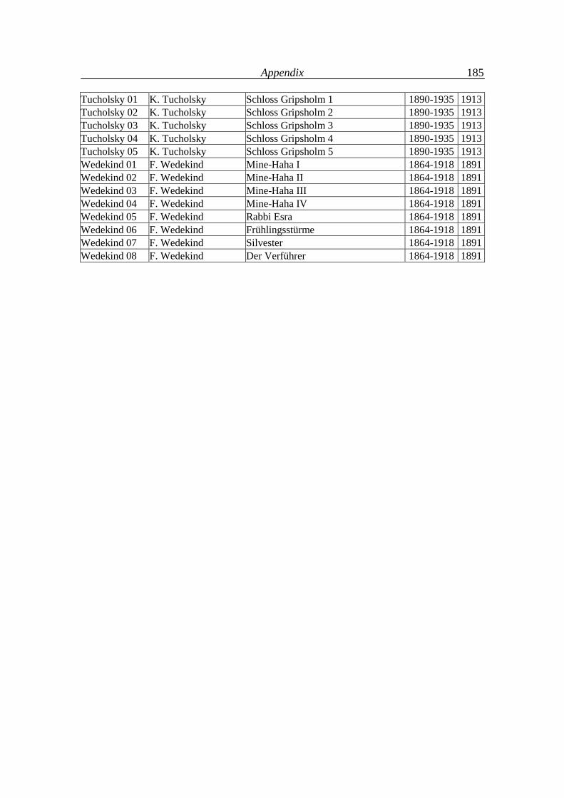
Appendix

185

Tucholsky 01 K. Tucholsky Schloss Gripsholm 1 1890-1935 1913 Tucholsky 02 K. Tucholsky Schloss Gripsholm 2 1890-1935 1913 Tucholsky 03 K. Tucholsky Schloss Gripsholm 3 1890-1935 1913 Tucholsky 04 K. Tucholsky Schloss Gripsholm 4 1890-1935 1913 Tucholsky 05 K. Tucholsky Schloss Gripsholm 5 1890-1935 1913 Wedekind 01 F. Wedekind Mine-Haha I 1864-1918 1891 Wedekind 02 F. Wedekind Mine-Haha II 1864-1918 1891 Wedekind 03 F. Wedekind Mine-Haha III 1864-1918 1891 Wedekind 04 F. Wedekind Mine-Haha IV 1864-1918 1891 Wedekind 05 F. Wedekind Rabbi Esra 1864-1918 1891 Wedekind 06 F. Wedekind Frühlingsstürme 1864-1918 1891 Wedekind 07 F. Wedekind Silvester 1864-1918 1891 Wedekind 08 F. Wedekind Der Verführer 1864-1918 1891

References Altmann, G. (1978). Zur Anwendung der Quotiente in der Textanalyse. Glot-

tometrika 1, 91-106. Altmann, G. (1988). Wiederholungen in Texten. Bochum: Brockmeyer. Altmann, G. (1992). Das Problem der Datenhomogenität. Glottometrika 13,

287-298. Altmann, G. (1999). Von der Fachsprache zum Modell. In: Wiegand, H.E. (ed.),

Sprache und Sprachen in den Wissenschaften- Geschichte und Gegenwart: 294-312. Berlin/New York: de Gruyter.

Altmann, G. (2001). Thery building in text science. In Uhlířová, L. et al. (eds.), Text as a linguistic paradigm: levels, constituents, constructs: 10-20. Trier: Wissenschaftlicher Verlag.

Altmann, G. (2005). Diversification processes. In: Köhler, R., Altmann, G., Piotrowski, R.G. (eds.), Quantitative Linguistics. An International Hand-book: 648-659. Berlin/New York: de Gruyter.

Altmann, G. (2006). Fundamentals of quantitative linguistics. In: Genzor, J., Bucková, M. (eds.), Favete linguis: 15-27. Bratislava: Slovak Academic Press.

Altmann,G., Best, K.-H., Kind, B. (1987). Eine Verallgemeinerung des Ge-setzes der semantischen Diversifikation. Glottometrika 8, 130-139.

Altmann, G., Lehfeldt, W. (1973).Allgemeine Sprachtypologie. München: Fink Beöthy, E., Altmann, G. (1984a). Semantic diversification of Hungarian verbal

prefixes. III. “föl-“, “el-“, “be-“. Glottometrika 7, 45-56. Beöthy, E., Altmann, G. (1984b). The diversification of meaning of Hungarian

verbal prefixes. II. ki-. Finnisch-Ugrische Mitteilungen 8, 29-37. Best, K.-H. (1991). Von: Zur Diversifikation einer Partikel des Deutschen. In:

Rothe (1991): 94-104. Best, K.-H. (1994). Word class frequencies in contemporary German short prose

texts. Journal of Quantitative Linguistics 1(2), 144-147. Best, K.-H. (2004/2005). Laut- und Phonemhäufigkeit im Deutschen. Göttinger

Beiträge zur Sprachwissenschaft 10/11, 21-32. Best, Karl-Heinz (2009). Zur Diversifikation deutscher Hexameter. Naukovyj

Visnyk Černivec’koho Universytetu: Hermans’ka filolohija. Vypusk 431, 172-180.

Best, K.-H. (2008). Zur Diversifikation lateinischer und griechischer Hexameter. Glottometrics 17, 45-53.

Bornmann, L., Daniel, H.-D. (2005). Does the h-index for ranking of scientists really work? Scientometrics, 65, 391-392.

Brüers, N., Heeren, A. (2004). Pluralallomorphe in Briefen Heinrich von Kleists. Glottometrics 7, 85-90.

Bunge, M. (1967). Scientific research I. Berlin-Heidelberg-New York: Springer.

References

187

Busemann, A. (1925). Die Sprache der Jugend als Ausdruck der Entwicklungs-rhythmik. Jena: Fischer.

Dietze, J. (1982). Grapheme und Graphemkombinationen der russischen Fach-sprache. Glottometrika 4, 80-94.

Drobisch, M.V. (1866). Ein statistischer Versuch über die Formen des latei-nischen Hexameters. Berichte über die Verhandlungen der Königlich Säch-sischen Gesellschaft der Wissenschaften zu Leipzig. Philologisch-histori-sche Classe 18, 73-139.

Drobisch, M.V. (1968a). Weitere Untersuchungen über die Formen des Hexa-meters der Vergil, Horaz und Homer. Berichte über die Verhandlungen der Königlich Sächsischen Gesellschaft der Wissenschaften zu Leipzig. Philo-logisch-historische Classe 20, 16-53.

Drobisch, M.V. (1968b). Über die Formen des deutschen Hexameters bei Klop-stock, Voss und Goethe. Berichte über die Verhandlungen der Königlich Sächsischen Gesellschaft der Wissenschaften zu Leipzig. Philologisch-historische Classe 20, 138-160.

Drobisch, M.W. (1872). Statistische Untersuchungen des Distichon (von Hrn. Dr. Hultgren). Berichte über die Verhandlungen der Königlich-Sächsischen Gesellschaft der Wissenschaften zu Leipzig, Philologisch-Historische Clas-se, 24, 1-33.

Drobisch, M.W. (1875). Ueber die Gesetzmässigkeit in Goethe’s und Schiller’s Distichen. Königlich-Sächsische Gesellschaft der Wissenschaften zu Leip-zig, Philologisch-Historische Classe, Berichte über die Verhandlungen 27, 8-34-146.

Egghe L. (2007a). Dynamic h-index: the Hirsch index in function of time. Journal of the American Society for Information Science and Technology, 58(3), 452-454.

Egghe L. (2007b). Item-time-dependent Lotkaian informetrics and applications to the calculation of the time-dependent h-index and g-index. Mathematical and Computer Modelling 45(7/8), 864-872.

Egghe L. (2008). The influence of transformations on the h-index and the g-index. Journal of the American Society for Information Science and Technology 59(8), 1304-1312.

Egghe L., Rao I.K.R. (2008). Study of different h-indices for groups of authors. Journal of the American Society for Information Science and Technology, 59(8),1276-1281.

Egghe, L., Rousseau, R. (2006). An informetric model for the Hirsch-index. Scientometrics 69(1), 121-129.

Esteban, M.D., Morales, D. (1995). A summary of entropy statistics. Kyber-netica 31(4), 337-346.

Fan, F., Popescu, I.-I., Altmann, G. (2008). Arc length and meaning diver-sification in English. Glottometrics 17, 82-89.

References

188

Fry, D.B. (1947). The frequency of occurrence of speech sounds in Southern English. Archives néerlandaises de phonétique expérimentale 20, 103-106.

Fuchs, R. (1991). Semantische Diversifikation der deutschen Präposition auf. In Rotthe (1991): 105-115.

Grigor´ev, V.I. (1980a). O dinamike raspredelenija bukv v tekste. In: Aktual´nye voprosy strukturnoj i prikladnoj lingvistiki. Sbornik statej: 40-48. Moskva.

Grigor´ev, V.I. (1980b). Frequency distribution of letters and their ranks in a running text. In: Symposium Computational Linguistics and Related Topics. Summaries: 43-47. Tallinn.

Grotjahn, R. (1982). Ein statistisches Modell für die Verteilung der Wortlänge. Zeitschrift für Sprachwissenschaft 1, 44-75.

Grzybek, P., Kelih, E. (2006). Towards a general model of grapheme frequen-cies for Slavic languages. In: Garabík, R. (Ed.), Computer Treatment of Slavic and East European Languages: 73-87.. Bratislava: Veda.

Grzybek, P., Kelih, E. (2003). Graphemhäufigkeiten (am Beispiel des Rus-sischen. Teil I. Methodologische Vor-Bemerkungen und Anmerkungen zur Geschichte der Erforschung von Graphemhäufigkeiten im Russischen. An-zeiger für Slavische Philologie 31, 131-162.

Hammerl, R., Sambor, J. (1991). Untersuchungen zur Verteilung der Bedeu-tungen der polyfunktionalen polnischen Präposition w im Text. In: Rothe (1991): 127-137

Hennern, A. (1991). Zur semantischen Diversifikation von „in“ im Englischen. In: Rothe (1991): 116-126.

Hirsch, J.E. (2005). An index to quantify an individual´s scientific research out-put. http://arxiv.org/PS_cache/physics/pdf/0508/0508025.pdf

Hřebíček, L. (1997). Lectures on text theory. Prague: Oriental Institute. Hřebíček, L. (2000). Variation in sequences. Prague: Oriental Institute. Hřebíček, L., Altmann, G. (1993). Prospects of text linguistics. In: Hřebíček,

L., Altmann, G. (eds.), Quantitative text analysis: 1-28. Trier: Wissen-schaftlicher Verlag.

Job, M. (1974). Untersuchungen zur Frequenz der Phoneme im Georgischen. Unveröffentlichte Seminararbeit, Ruhr-Universität Bochum.

Joos, M. (1936). Review of G.K. Zipf, The Psycho-Biology of Language. Language 12, 196-210.

Kalinina, E.A. (1968). Izučenie leksiko-statističeskich zakonomernostej na osnove vjerojatnostnoj modeli. In: Statistika reči 64-107. Lenngrad.

Kaliu�čenko, V.D. (1988). Deutsche denominale Verben. Tübingen: Narr. Kuße, H. (1991). A und no in N.M. Karamzins Pis´ma Russkogo Putešestven-

nika. In: Rothe (1991): 173-182. Liu, Y., Rousseau, R. (2008). Definitions of time series in citation analysis with

special attention to the h-index . Journal of Informetrics, 2(3), 202-210. Mačutek, J., Popescu, I.-I., Altmann, G. (2007). Confidence intervals and tests

for the h-point and related text characteristics. Glottometzrics 15, 42-52.

References

189

Meier, H. (1964). Deutsche Sprachstatistik. Hildesheim: Olms. Meuser, K., Schütte, J.M., Stremme, S. (2008). Pluralallomorphe in den Kurz-

geschichten von Wolfdietrich Schnurre. Glottometrics 17, 2008, 20-25. Nemcová, E. (1991). Semantic diversification of Slovak verbal prefixes. In: Ro-

the (1991): 67-74. Nemcová, E. (2007). Zur Diversifikation des Bedeutungsfeldes slowakischer

verbaler Präfixe. In: Grzybek, P., Köhler, R. (eds.), Exact methods in the study of language and text: 499-508. Berlin/New York: Mouton de Gruyter.

Nemcová, E., Popescu, I.-I., Altmann, G. (2009). Word associations in French. (submitted).

Oehlert, G.W. (1992). A note on the delta method. The American Statistician 46, 27-29

Ol´chin, P. (1907). Pervaja opora pri postroenii racional´noj stenografii. Steno-graf 4-5, 114-118.

Ord, J.K. (1972). Families of frequency distributions. London: Griffin, Orlov, J.K., Boroda, M.G., Nadarejšvili, I.Š. (1982). Sprache, Text, Kunst.

Quantitative Analysen. Bochum: Brockmeyer. Pääkkönen, M. (1994). Graphemes and context: statistical data on the graph-

ology of standard Finnish. Glottometrika 14, 1-53. Pawlowski, A. (1999). The quantitative approach in cultural anthropology: Ap-

plication of linguistic corpora in the analysis of basic colour terms. Journal of Quantitative Linguistics 6(3), 222-234.

Popescu, I.-I. (2007). Text ranking by the weight of highly frequent words. In: Grzybek, P., Köhler, R. (eds.), Exact methods in the study of language and text: 555-565. Berlin/New York: Mouton de Gruyter.

Popescu, I.-I., Altmann, G. (2006a). Some geometric properties of word fre-quency distributions. Göttinger Beiträge zur Sprachwissenschaft 13, 87-98.

Popescu, I.-I., Altmann, G., (2006b). Some aspects of word frequencies. Glotto-metrics 13, 2006, 23-46.

Popescu, I.-I., Altmann, G. (2007). Writer´s view of text generation. Glotto-metrics 15, 42-52.

Popescu, I.-I., Altmann, G. (2007a). On the diversity of word frequencies and language typology. Göttinger Beiträge zur Sprachwissenschaft 14, 81-91.

Popescu, I.-I., Altmann, G. (2008). Autosemantic compactness of text. In: Alt-mann, G., Zadorozhna, I., Matskulyak V. (eds.), Problems in General, Ger-manic and Slavic Linguistics. Papers for 70th anniversary of Professor V. Levickij: 427-480. Chernivtsi: Books – XXI.

Popescu, I.-I., Altmann, G. (2008a). Hapax legomena and language typology. Journal of Quantitative Linguistics 15(4), 370-378. .

Popescu, I.-I., Altmann, G. (2008b). Zipf´s mean and language typology. Glottometrics 16, 31-38.

Popescu, I.-I., Altmann, G., Köhler, R. (2009). Zipf´s law – another view. Quality and Quantity Online 9.5.2009.

References

190

Popescu, I.-I., Best, K.-H., Altmann, G. (2007) On the dynamics of word classes in text. Glottometrics 14, 58-71.

Popescu, I.-I., Mačutek, J., Altmann, G. (2008). Word frequency and arc length. Glottometrics 17, 18-44.

Popescu, I.-I., Altmann, G., Grzybek, Jayaram, B.D., Köhler, R., Krupa, V., P., Mačutek, J., Pustet, R., Uhlířová, L., Vidya, M.N., (2009). Word frequency studies. Berlin/ New York: Mouton de Gruyter.

Proskurin, N. (1933). Podsčety častoty liter i komplektovka �rifta. In: Revolju-cija i pis´mennost´. Sbornik I: 72-82. Moskva-Leningrad.

Rademacher, A. (1974). Untersuchungen zu den Buchstabenhäufigkeiten des See-Dajakischen. Unveröffentlichte Seminararbeit, Ruhr-Universistät Bo-chum

Roos, U. (1991). Diversifikation der japanischen Postposition „-ni“. In: Rothe (1991): 75-82.

Rothe, U. (1986). Die Semantik des textuellen et. Frankfurt: Lang. Rothe, U. (1990). Semantische Beziehungen zwischen Präfixen deutscher

denominaler Verben und den motivierenden Nomina. Glottometrika 11, 111-121.

Rothe, U. (ed.) (1991). Diversification processes in language: grammar. Hagen: Rottmann.

Rothe, U. (1991a). Diversification of the case in German: genitive. In Rothe (1991): 140-156.

Rothe, U. (1991b). Diversification processes in grammar: an introduction. In: Rothe (1991): 3-32.

Rousseau, R. (2007). The influence of missing publications on the h-index. Journal of Informetrics 1(1), 2-7.

Sambor, J. (1989). Polnische Version des Projekts “Sprachliche Synergetik. Teil I. Quantitative Lexikologie. Glottometrika 10, 171-197.

Schulze, E. (1974). Untersuchungen zu den Buchstabenhäufigkeiten des Hawaii-schen. Unveröffentlichte Seminararbeit, Ruhr-Universistät Bochum

Schweers, A., Zhu, J. (1991). Wortartenklassifizierung im Lateinischen, Deut-schen und Chinesischen. In: Rothe (1991): 157-165.

Thérouanne, P. Denhière, G. (2004). Normes d'association libre et fréquences relatives des acceptions pour 162 mots homonymes. L'Année Psy-chologique 104, 537-595.

Tuzzi, A., Popescu, I.-I., Altmann, G. (2009). Associative analyis of Italian presidential addresses (submitted)

Wimmer, G., Altmann, G. (19996). The theory of word length: some results and generalizations. Glottometrika 15, 112-133.

Wimmer, G., Altmann, G., Hřebíček, L., Ondrejovič, S., Wimmerová, S. (2003). Úvod do analýzy textov. Bratislava: Veda.

References

191

Wimmer, G., Witkovský, V., Altmann, G. (1999). Modification of probability distributions applied to word length research. Journal of Quantitative Lin-guistics 6, 257-268.

Yngve, V. H. (1961). The depth hypothesis. In: Jakobson, R. (ed.), Structure of language and its mathematical aspects: 130-138. Providence, R.I.

Ziegler, A. (1998). Word class frequencies in Brazilian-Portuguese press texts. Journal of Quantitative Linguistics 5(3), 269-280.

Ziegler, A. (2001). Word class frequencies in Portuguese press texts. In: Uhlí-řová, L. et al. (eds.), Text as a linguistic paradigm: levels, constituents, con-structs. Festschrift in honour of Luděk Hřebíček: 294-312. Trier: Wissen-schaftlicher Verlag

Ziegler, A., Best, K.-H., Altmann, G. (2002). Nominalstil. ETC – Empirical Text and Culture Research 2, 72-85.

Author index Altmann, G. 3,6,9,10,14,16,17,25- 27,33,48,50,56,64,66.68,69, 73,75, 85,86,94,95,99,102, 106,111,119,120,172-174,177 Aristotle 177 Bacon, F. 6 Beöthy, E. 85 Best, K.-H. 26,73,80,85,174 Bornman,L. 24 Boroda, M.G. 171 Brüers, N. 77,78 Bunge, M. 4 Busemann, A. 171,172 Cramér, H. 16 Cressie, N. 15 Daniel, H.-D. 24 Denhière, G. 95 Dietze, J. 73 Drobisch, M.V. 73,74 Egghe, L. 24 Esteban, M.D. 157 Fan, F. 86,94 Fry, D.B. 71 Fuchs, R. 80 Grigor´ev, V.I. 72 Grotjahn, R. 9 Grzybek, P. 71 Hammerl, R. 80 Heeren, A. 77,78 Hennern, A. 80 Hirsch, J.E. 24,144 Hřebíček, L. 2,3,8 Job, M. 72 Joos, M. 15 Kalinina, E.E. 72 Kaliu�čenko, V.D. 85 Kelih, E. 71,94 Kind, B. 85 Köhler, R. 10,14,16,17,91,99 Kuße, H. 80 Lehfeldt, W. 177

Li, W. 13 Liu, Y. 24 Mačutek, J. 26,50,56,64,66,68,75,99, 156 Mandelbrot, B. 13 Martináková, Z. 75 Meier, H. 72 Meuser, K.77,78 Morales, D. 157 Nadarejšvili, I.Š. 171 Nemcová, E. 85,95 Oehlert, G.W. 51 Ol´chin, P. 72 Ord, J.K. 161 Orlov, J.K. 9,171 Pääkkönen, M. 72 Pawlowski, A. 77 Pearson, K. 16 Popescu, I.-I. 10,14,16,17,24-27,33, 48,50,56,64,66,68,69,73,75, 86,94, 95,99,102,106,111,119, 122,156,167 Proskurin, N. 72 Rademacher, A. 72 Rao, I.K. 24 Read, T.R.C. 15 Roos, U. 80 Rothe, U. 85,94,95 Rousseau, R. 24 Sambor, J. 73,79,80 Schnurre, W. 77 Schulze, E. 72 Schütte, J.M. 77,78 Schweers, A. 73 Stremme, S. 77,78 Tesnière, L. 177 Thérouanne, P. 95 Tschuproff, A.A. 16 Tuzzi, A. 26,48,73,94,119 Wimmer, G. 5,6,9,14 Witkovský, V. 9

Author index

193

Yingve, V. 177 Zhu, J. 73

Ziegler, A. 73,1, A.74 Zipf, G.K. 13,15,20,66

Subject index affix 69 analogy 13 analysis, - classificatory 6 - comparative 6 - descriptive 6 - global 6 - historical 6 - sequential 6 - theoretical 6 arc development 64-67 arc length 49-98,100,132 attractor 33,47,48 autosemantic13-15,25,26 auxiliary 69,79,80,96,97,99 axiom 1,4 category, Aristotelian 177 category, grammatical 95 change 3 chi-square 15,16 class, - colour 69,77 - paradigmatic 69,78,79,96 classification 1,26,28,33-40,49, 166,173 - biangular 26,34,36-40 - grammatical 71 - triangular 26 coefficient, - of contingency 16 - of determination 16,20 compactness, autosemantic 26 concentration, thematic 25,26 concept 1,4-6,12,15 - qualitative 2,7 - quantitative 2,6,7 confirmation 4 continuity 15 convention 1,3 Cressie-Read statistics 15 criterion 3,4,12

- external 4 crowding 26 dactyl 74 data 13 deduction 6 definition 1,3 - operational 3,4 description 1,7 deviation 15,16 - normal 15 - unexplained 16 discreteness 15 distance, Euclidian 49 distribution 3 - binomial 172,173,174 - discrete 15 - gamma 9 - multinomial 52 - negative binomial 9 - normal 15,174 - Poisson 9 - rank-frequency 3,10,11,14,70, 83 - sentence length 13 - word length 9 - Zipf (zeta) 10,13 divergence 172 diversification, semantic 85,86,94, 96,97 diversity, word frequency 157-170 dogmatism 178 economy 4 entropy 157-170 - relative 157 - variance of 157 equilibrium 26,172,174,176 - nominal-verbal 173 feature, suprasegmental 73 fixed-point 24 frequency, word-form 13 function 1

Subject index

195

- exponential 13,14,20,111,131 - power 66 - Zipfian 104-106,111,112 generality 4 golden section 48,119,156 hapax legomena 99-111 hexameter 73 hierarchy 2 Hirsch coefficient a 144 homogeneity 8-13,15 h-point 24-48,132 hypothesis 1,4,6,12,13 - active 4 - global 4 - inductive 4 - lawlike 5 - local 4 - low-level 4 - probabilistic 4 - statistical 4 - textual 4 idola 6,7 indicator - b 144-156 - B1 50,53,56,59,60 - B2 50,53,56,61,62 - B3 50,54,56,62-65 - B4 51,54,56,62,64 - B5 100-105 - B6 106-110,112,115-118 - B7 111,112,115,116 - B8 112,115,116,117 - B9 112,115,117,118 - B10 118 - c 69,71-98 - I1 171,172 - p 68-98,144-156 - q 144-156 - θ 118-131 - typological 49,66 inventory 15,22 language,

- analytic 36,99,101,104,111,112, 123,134,160, 166,170 - Brazilian Portuguese 73 - Bulgarian 17,20,28,33,41,47,48, 57, 61, 63,91,100,102,105,106, 109,112,115,120,122,131,134, 145,156,157,160,161,166,167, 169 - Chinese 73 - Czech 17,28,29,33,41,47,57, 60,61,63,77,91,100,102,106, 109,112,115,120,122,131, 134,145,156, 157,160-162, 166,168,169 - Early High German 13 - English 4,8,17,23,29,33,42,47, 57,61,63,71,72,77,80,86-91, 94,100,102,106,109,112,113, 115,120,122,131,132,134,143, 145,156,157,160,162,166,168, 169 - Finnish 72 - French 66,77,94-97 - Georgian 72 - German 9,17,21-23,29,33,42, 47,48,57,61,63-67,69,73,76, 77,80, 81,85, 86,91,92,95,100, 102,106,107,109,115,120,122, 124,125,130-132,134-143, 145,148-156, 158-160,162, 166,168,169,174 - Greek 69,73,96,97,177 - Hawaiian 17,18,22,30,33,47, 57,61,63,72,92,101,102,105, 107,109,111-113,115,120- 122,124-126, 130-132,134, 145,156,159,160,162,163,166, 169 - Hungarian 17,22,29,30,33, 42, 43,47,57,60,61, 63,85,92,100 -102,104,107,109,113,115, 120,122,132,134,145,156, 159,160,162, 166,169

Subject index

196

- Indonesian 18,22,30,33,36, 43, 47,48,58,61,62,92,101,102, 107,109,113,115,121,122, 132,134,145,156,159,160, 163,166,169 - isolating 48 - Italian 18,30,33,43,47,57,58, 60,61,63,77,92,94,96,97,101, 102,107,109,113,115,121, 122,132,134,145,156,159,160, 163,166,169 - Japanese 80 - Kannada 18,21,30,33,43,47, 58,60, 61,62,92,101,102,107, 109,113,115,121-124,126, 127,132,134, 145,156,158- 160,163,166,167,169 - Lakota 18,21,30,33,43,47,48, 58,61,63, 92,100,102,107, 109,113,115,120,121,122, 132-134,145, 156,158,160, 163,166-169 - Latin 18,30,33,43,47,58,60, 61,63, 66,69,73,96,100,102, 107,109,113,114,115,120, 122,133,134, 145,156,158, 160,163,166,168,169 - Maori 18,21,30,33,43,47,58, 61,63,92,100,102,107,109, 114,115,120,122,133,134, 145,156,158,160,163,164, 166,168,169 - Marathi 18,31,33,44,45,47,60, 61,63,93,100,102,108,109, 114,115,120,122,123,124, 128,129,133,134,145,156, 158-160,164,166,168,169 - Marquesan 18,31-33,43,44,47, 58,61, 63,93,100,102,107- 109,114,115,120,122,123, 124,127,128,131,133,134, 145,156,158, 160,164,166, 168,169

- Middle High German 85 - Polish 69,73,77,79,80 - Polynesian 59,108,122,160 - Portuguese 73 - Rarotongan 19,21,32,33,45,47, 59,61,63,93,101,102, 108,109, 114,115,120,122,133,134,147, 156,159,160,164,166,169 - Romanian 19,32,33,45,47,58, 60,61,63,77,93,100-102,108, 109,114,115,120,122,133, 134,147,156-160,164,166, 168,169 - Russian 19,22,32,33,45,47,59- 61,63,71,72,77,80,93,101, 102,108,109,114,115,121,122, 133,134,147,156,159,160,164, 166,169 - Samoan 19,22,32,33,45,47,59, 61,63,93,101,102,108,109, 114,115,121,122,134,147,156, 159,160,165,166,169 - Sea Dayak 72 - Serbian 72 - Slavic 3,94,96,97 - Slovak 3,72,77,85,86 - Slovenian 19,22,32,33,45,47, 59,60, 63,72,93,101,102,108, 109,114,115,121,122133,134, 147,159,160,164-166,169 - Spanish, 77 - synthetic 36,66,99,101,104, 111,134,156,160,166,170 - Tagalog 19,22,32,33,36,45,47, 59,61,63,93,101,102,108,109, 115,121,122,134,147,156,159, 160,165,166,169 - typology 47,111-156 - Ukrainian 77 - level 70- law 2,4 - allometric 8 - Menzerath´s 2,8

Subject index

197

- textological 7 - Zipf´s 13-23, - Zipf-Mandelbrot´s 8 letter 69,71,72,96,97 linguistics, synergetic 6 measurement 13 method, quantitative 6 nominality 173-176 operation 3 operationalization 2,3 pace filling, autosemantic 26 parts-of-speech 8,10,13 pattern, rhythmic 69,96,97 phoneme 69,71,96,97 pitch 69,75,96 plot, ternary 46-48 predicate 177 probability 5 - conditional 52 process 1,7 property 1-3,5-8,13,15,68,171 - "natural" 3 - external 2 - isolated 3 proto-science 1 reference 25 regularity 15 relation 1,6,7 repeat rate 157-170 requirement 4 richness, form 99 - vocabulary 99 rule 3 sample size 16 sampling 8-12 - authoritative 12 - random 12 - systematic 12 scheme - <I,J> 161 - Ord´s 161 self-regulation 3,4,26,48 sentence

- centrality 177 - dependence 177 - depth 177 - width 177 sequence 2,15,16,174 - decreasing 15 - geometric 13 - rank-frequency 3,16,22,49,71, 99,131 - Zipf´s zeta 20 shape factor 131-143 simplification 7 sound 69,71,72,96,97 speech act 1,178 spondee 74 stratification 12,22 stratum 11,14 structure 1,3,7 style, - active 171 - descriptive 171 - nominal 171-178 - ornamental 171 superposition 10,14 symbol 3 symmetry 4 synsemantic 13-15,25,26 system 1,4,6,7 Taylor polynomial 51 test - binomial 177 - goodness-of-fit 15,16 - statistical 1,8 text - classification 40 - interpreted 2 - musical 1 - written 2 theory 1-7 - axiomatized 5 - inductive-deductive 4 - partial 1 thing 1

Subject index

198

typology - language 6,157-70 - text 6 uncertainty 160 uniformity 160 unit, rhythmic 73 variation 16 verbality 173,174,177 view - autosemantic 27,34 - synsemantic 28,34 - wirter´s 26,27,33 word association 69,95 word class 69,73,96 word-form 2,3,22,80,81,91-94, 99,165