Embed Size (px)
Citation preview
STT 315
This lecture is based on Chapter 4.6-4.11.
Acknowledgement: Author is thankful to Dr. Ashok Sinha, Dr. Jennifer Kaplan and Dr. Parthanil Roy for allowing him to use/edit some of their slides.
2
Normal Distribution
3
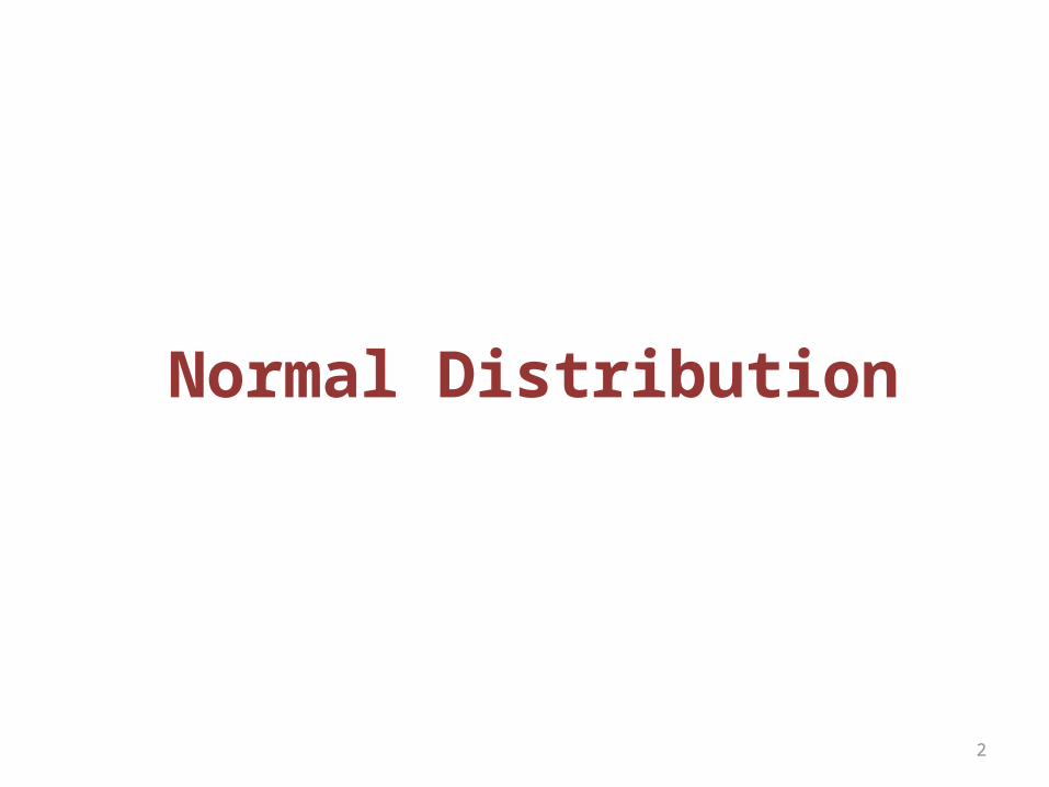
Normal random variableA normal random variable X
– is a continuous random variable– has a probability distribution which is bell-shaped,
i.e.,• unimodal,• symmetric.
• In many data-sets, the histogram is bell-shaped. These data-sets can be modeled using normal distribution.
4
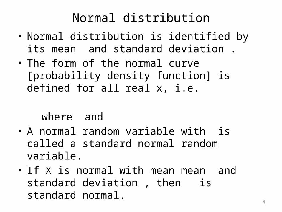
Normal distribution• Normal distribution is identified by its mean and
standard deviation .• The form of the normal curve [probability density
function] is defined for all real x, i.e.
where and • A normal random variable with is called a standard
normal random variable.• If X is normal with mean mean and standard
deviation , then is standard normal.
5
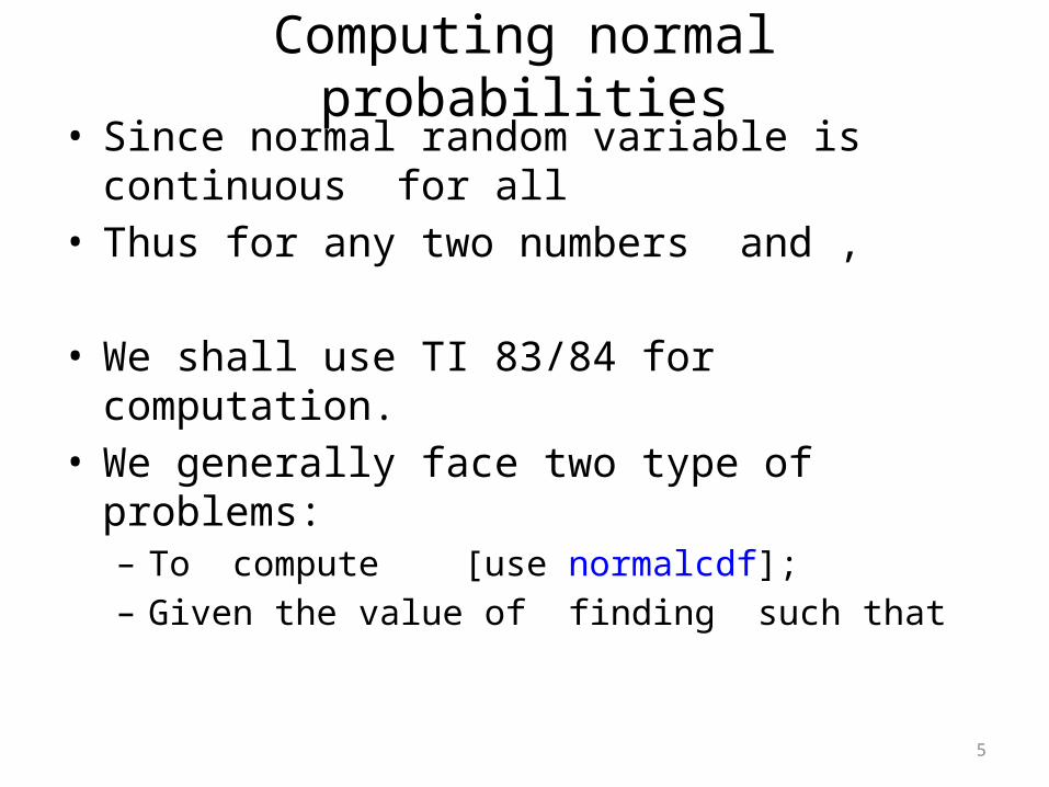
Computing normal probabilities• Since normal random variable is continuous for all • Thus for any two numbers and ,
• We shall use TI 83/84 for computation.• We generally face two type of problems:
– To compute [use normalcdf];– Given the value of finding such that
6
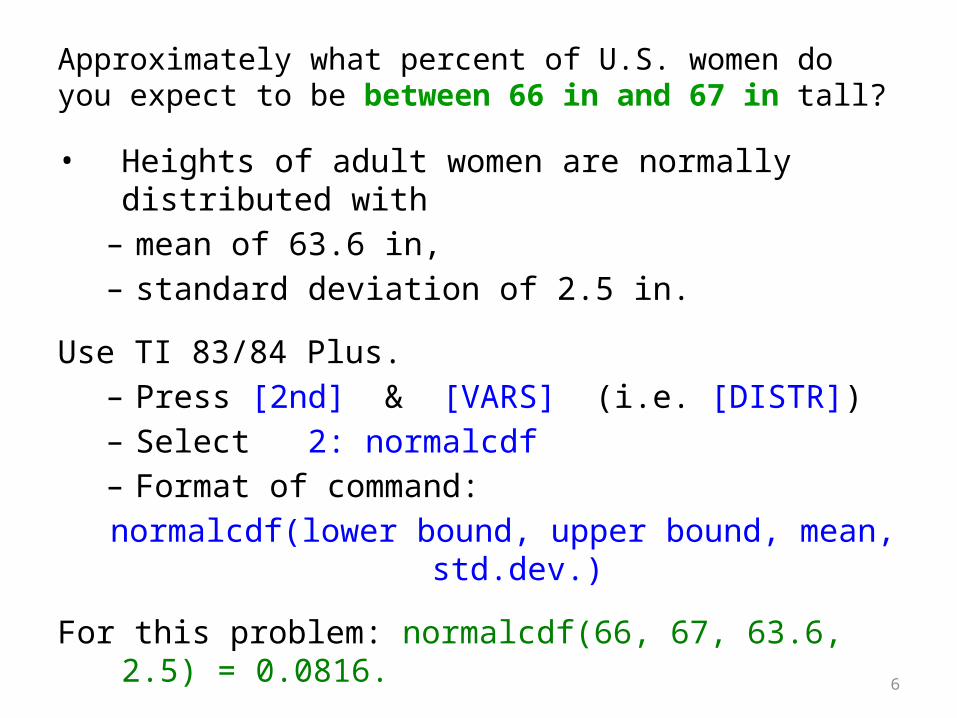
Approximately what percent of U.S. women do you expect to be between 66 in and 67 in tall?
• Heights of adult women are normally distributed with– mean of 63.6 in,– standard deviation of 2.5 in.
Use TI 83/84 Plus. – Press [2nd] & [VARS] (i.e. [DISTR])– Select 2: normalcdf– Format of command:
normalcdf(lower bound, upper bound, mean, std.dev.)
For this problem: normalcdf(66, 67, 63.6, 2.5) = 0.0816.
i.e. about 8.2% of adult U.S. women have heights between 66 in and 67 in.
7
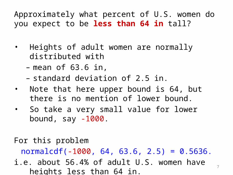
Approximately what percent of U.S. women do you expect to be less than 64 in tall?
• Heights of adult women are normally distributed with– mean of 63.6 in,– standard deviation of 2.5 in.
• Note that here upper bound is 64, but there is no mention of lower bound.
• So take a very small value for lower bound, say -1000.
For this problemnormalcdf(-1000, 64, 63.6, 2.5) = 0.5636.
i.e. about 56.4% of adult U.S. women have heights less than 64 in.

8
Approximately what percent of U.S. women do you expect to be more than 58 in tall?
• Heights of adult women are normally distributed with– mean of 63.6 in,– standard deviation of 2.5 in.
• Note that here lower bound is 58, but there is no mention of upper bound.
• So take a very high value for upper bound, say 1000.
For this problemnormalcdf(58, 1000, 63.6, 2.5) = 0.987.
i.e. 98.7% of adult U.S. women have heights more than 58 in.
9
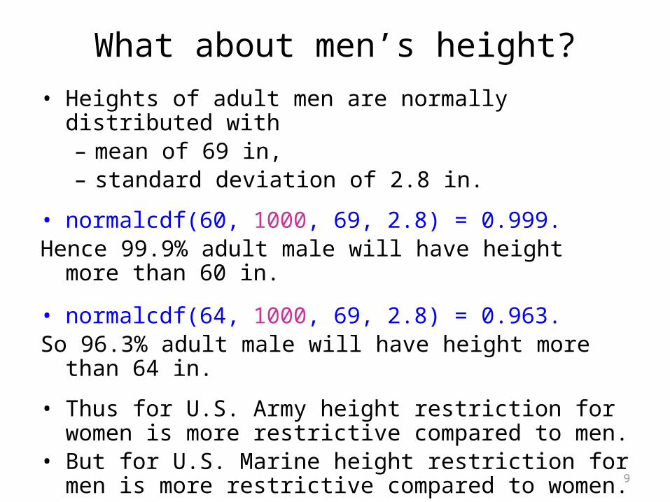
What about men’s height?• Heights of adult men are normally distributed with
– mean of 69 in,– standard deviation of 2.8 in.
• normalcdf(60, 1000, 69, 2.8) = 0.999.Hence 99.9% adult male will have height more than 60 in.
• normalcdf(64, 1000, 69, 2.8) = 0.963.So 96.3% adult male will have height more than 64 in.
• Thus for U.S. Army height restriction for women is more restrictive compared to men.
• But for U.S. Marine height restriction for men is more restrictive compared to women.
10
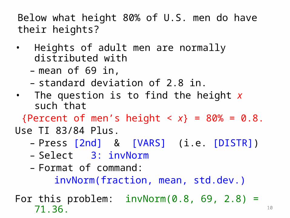
Below what height 80% of U.S. men do have their heights?
• Heights of adult men are normally distributed with– mean of 69 in,– standard deviation of 2.8 in.
• The question is to find the height x such that {Percent of men’s height < x} = 80% = 0.8.
Use TI 83/84 Plus. – Press [2nd] & [VARS] (i.e. [DISTR])– Select 3: invNorm– Format of command:
invNorm(fraction, mean, std.dev.)
For this problem: invNorm(0.8, 69, 2.8) = 71.36.
i.e. 80% of U.S. men have heights less than 71.36 in.
11
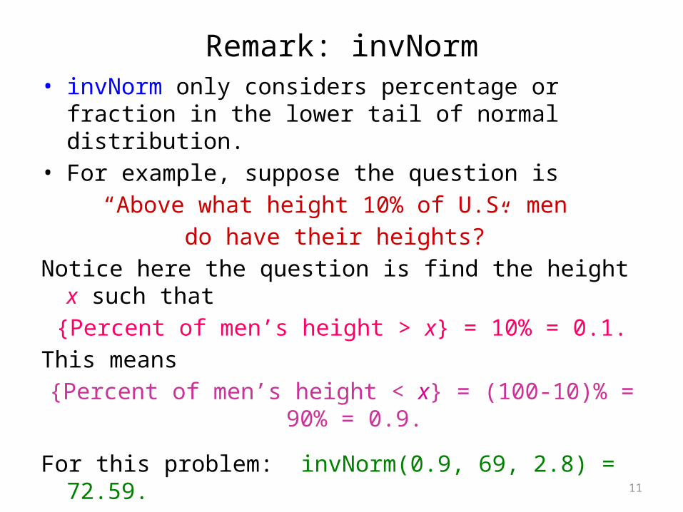
Remark: invNorm• invNorm only considers percentage or fraction in the lower
tail of normal distribution.• For example, suppose the question is
“Above what height 10% of U.S. men do have their heights?”
Notice here the question is find the height x such that{Percent of men’s height > x} = 10% = 0.1.
This means{Percent of men’s height < x} = (100-10)% = 90% = 0.9.
For this problem: invNorm(0.9, 69, 2.8) = 72.59.
i.e. 90% of U.S. men have heights less than 72.59 in,i.e. 10% of U.S. men have heights more than 72.59 in.

12
Normal approximation of binomial distribution
Suppose Hence
If n is very large, then the probability distribution of X can be approximated by normal distribution with
However, X being binomially distributed is a discrete random variable, whereas normal distribution is continuous. So we need a continuity correction.
If n is very large, then we compute as follows:
13
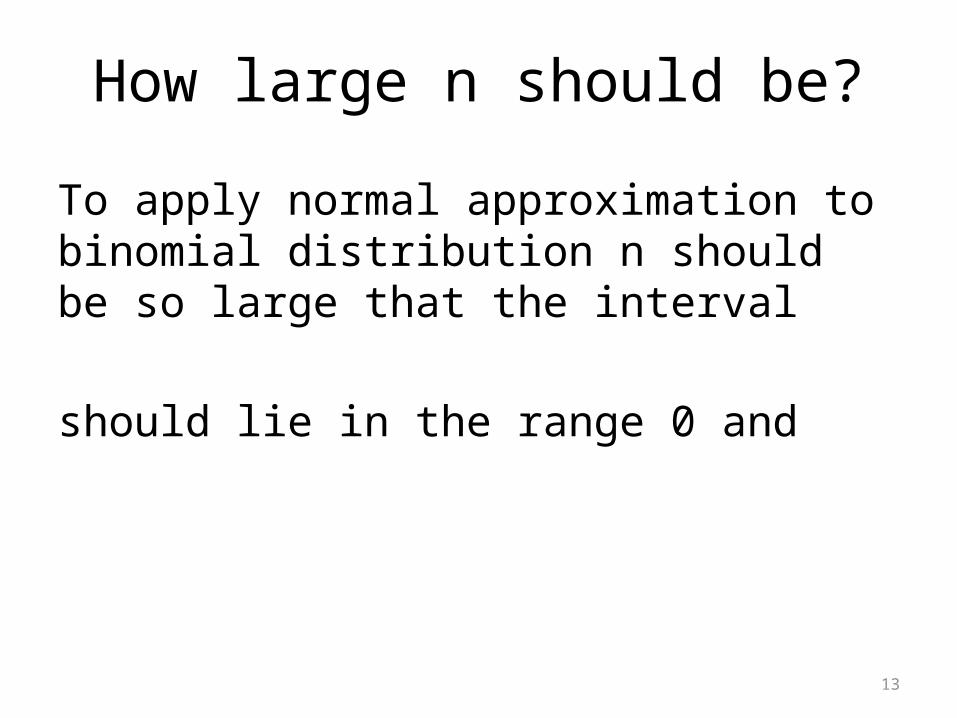
How large n should be?
To apply normal approximation to binomial distribution n should be so large that the interval
should lie in the range 0 and
14
ExampleLet X be binomially distributed with Here .Thus which lies in the range 0 and . Hence n is large enough.
15
ExampleSuppose X is normally distributed with mean and standard deviation . What is the probability that the value of X will be within 1.5 standard deviation from the mean? i.e. Solution: Remember that is standard normal.The z-score of is andthe z-score of is So, normalcdf(-1.5,1.5,0,1)=0.8664.
16
Sum of independent random variables
17
Combining Random Variables• Let X and Y be two random variables. Then
• If further X and Y are independent, then
• Notice that for variance both have a “plus” sign on the right hand side.
• For expectation, “independence” assumption is not necessary, but for the above variance formula it is required.
• Variance for “dependent” case will not be treated in this course.
18
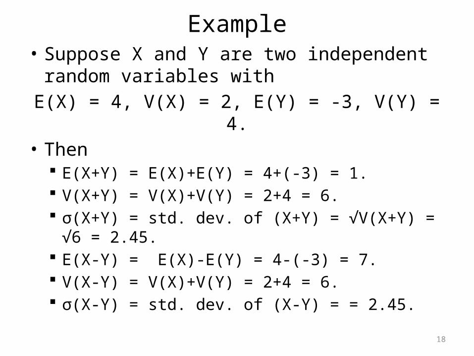
Example• Suppose X and Y are two independent random
variables withE(X) = 4, V(X) = 2, E(Y) = -3, V(Y) = 4.
• Then E(X+Y) = E(X)+E(Y) = 4+(-3) = 1. V(X+Y) = V(X)+V(Y) = 2+4 = 6. σ(X+Y) = std. dev. of (X+Y) = √V(X+Y) = √6 = 2.45. E(X-Y) = E(X)-E(Y) = 4-(-3) = 7. V(X-Y) = V(X)+V(Y) = 2+4 = 6. σ(X-Y) = std. dev. of (X-Y) = = 2.45.
19
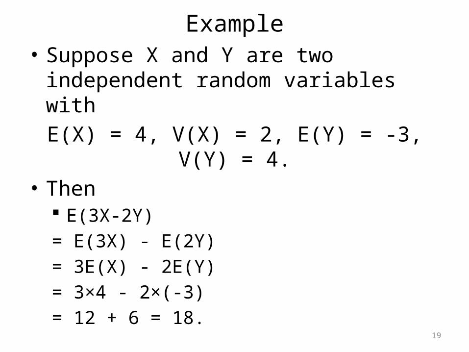
Example• Suppose X and Y are two independent random
variables withE(X) = 4, V(X) = 2, E(Y) = -3, V(Y) = 4.
• Then E(3X-2Y) = E(3X) - E(2Y) = 3E(X) - 2E(Y) = 3×4 - 2×(-3) = 12 + 6 = 18.
20
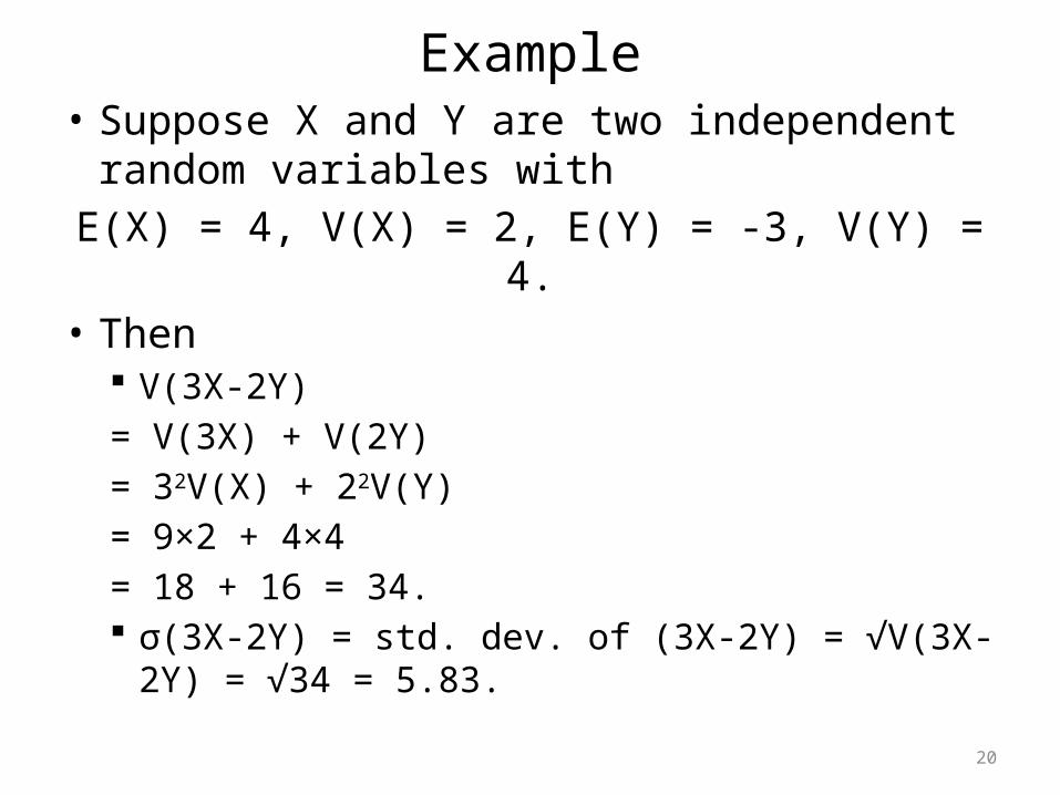
Example• Suppose X and Y are two independent random
variables withE(X) = 4, V(X) = 2, E(Y) = -3, V(Y) = 4.
• Then V(3X-2Y) = V(3X) + V(2Y) = 32V(X) + 22V(Y) = 9×2 + 4×4 = 18 + 16 = 34. σ(3X-2Y) = std. dev. of (3X-2Y) = √V(3X-2Y) = √34 =
5.83.
21
Example
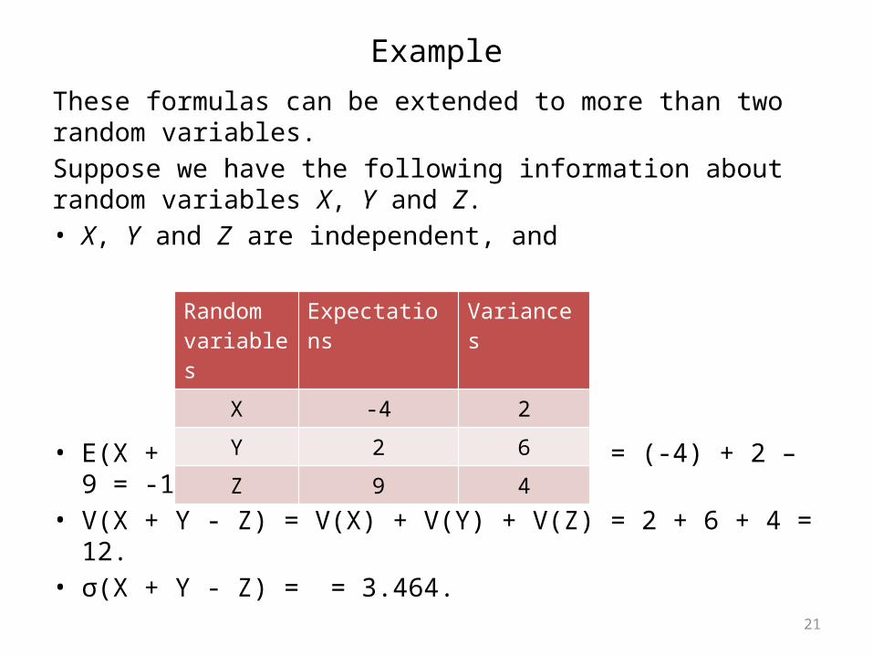
These formulas can be extended to more than two random variables. Suppose we have the following information about random variables X, Y and Z.• X, Y and Z are independent, and
• E(X + Y - Z) = E(X) + E(Y) – E(Z) = (-4) + 2 – 9 = -11.• V(X + Y - Z) = V(X) + V(Y) + V(Z) = 2 + 6 + 4 = 12.• σ(X + Y - Z) = = 3.464.
Random variables
Expectations Variances
X -4 2
Y 2 6
Z 9 4
22
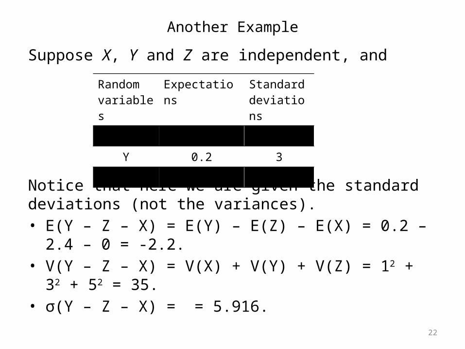
Another Example
Suppose X, Y and Z are independent, and
Notice that here we are given the standard deviations (not the variances).• E(Y – Z – X) = E(Y) – E(Z) – E(X) = 0.2 – 2.4 – 0 = -2.2.• V(Y – Z – X) = V(X) + V(Y) + V(Z) = 12 + 32 + 52 = 35.• σ(Y – Z – X) = = 5.916.
Random variables
Expectations Standard deviations
X 0 1
Y 0.2 3
Z 2.4 5
23
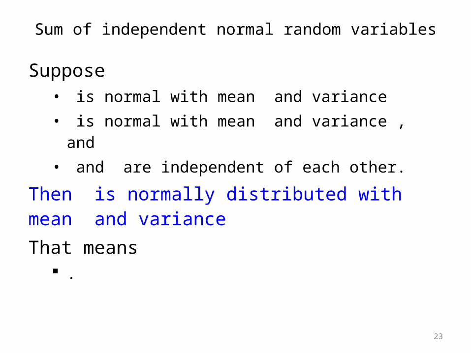
Sum of independent normal random variables
Suppose• is normal with mean and variance • is normal with mean and variance , and• and are independent of each other.
Then is normally distributed with mean and variance That means
.
24
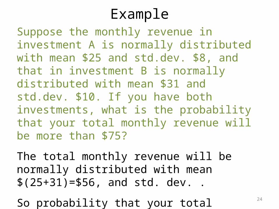
ExampleSuppose the monthly revenue in investment A is normally distributed with mean $25 and std.dev. $8, and that in investment B is normally distributed with mean $31 and std.dev. $10. If you have both investments, what is the probability that your total monthly revenue will be more than $75?
The total monthly revenue will be normally distributed with mean $(25+31)=$56, and std. dev. .
So probability that your total monthly revenue will be more than $75 is = normalcdf(75,1000,56,12.806) = 0.069.
25
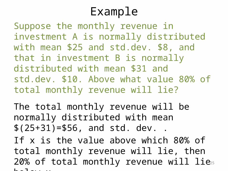
ExampleSuppose the monthly revenue in investment A is normally distributed with mean $25 and std.dev. $8, and that in investment B is normally distributed with mean $31 and std.dev. $10. Above what value 80% of total monthly revenue will lie?
The total monthly revenue will be normally distributed with mean $(25+31)=$56, and std. dev. .If x is the value above which 80% of total monthly revenue will lie, then 20% of total monthly revenue will lie below x.Thus x = invNorm(0.2,56,12.806) = $45.83.
26
Uniform distribution
27
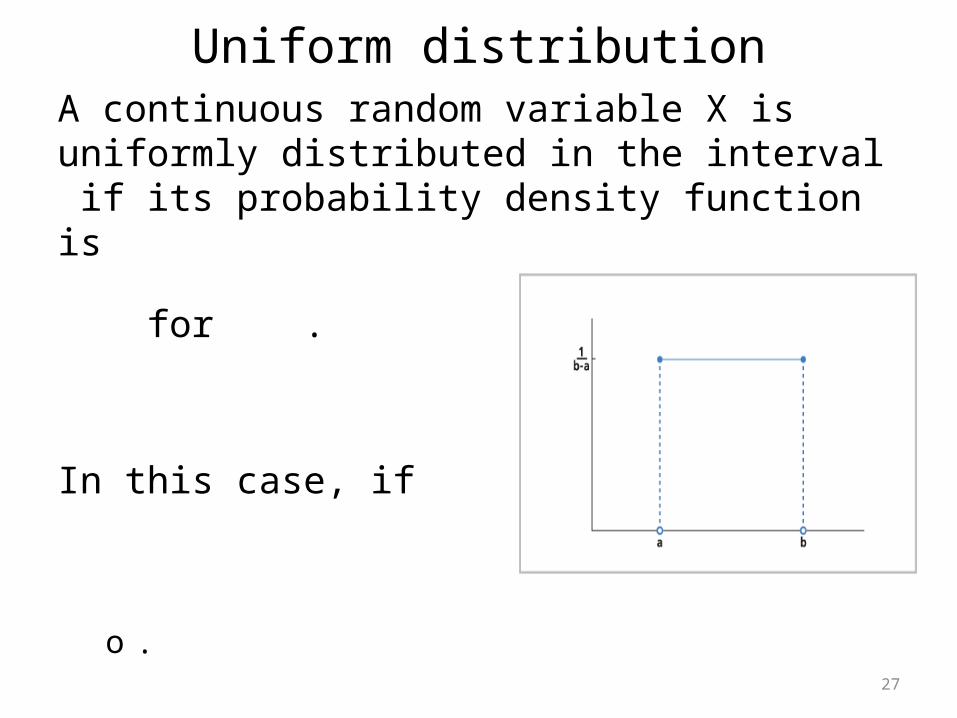
Uniform distributionA continuous random variable X is uniformly distributed in the interval if its probability density function is
for .
In this case, if
o .
28
ExampleIf price of gas (X) in East Lansing has uniform distribution in the interval $[3.45, 3.95] per gallon. • Probability that gas price will be between $3.50 and $3.60
• Probability that gas price will be less than $3.70
• Probability that gas price will be more than $3.90
• Probability that gas price will be $3.82 , because X is a continuous random variable.
29
ExampleIf price of gas (X) in East Lansing has uniform distribution in the interval $[3.45, 3.95] per gallon.
• The expected gas price in East Lansing is
• The standard deviation of gas price in East Lansing is
30
Exponential distribution
31
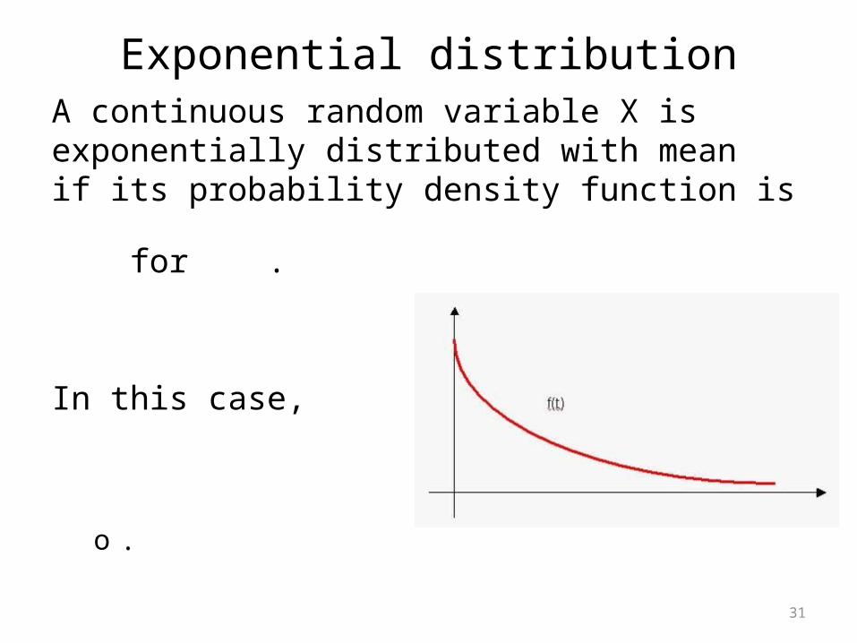
Exponential distributionA continuous random variable X is exponentially distributed with mean if its probability density function is
for .
In this case,
o .
32
ExampleIf the waiting time (X) for Bus #1 is exponentially distributed with mean 10 min.
Chance that we will get a Bus #1 within next 5 min Chance that we have to wait more than 20 min for
bus #1 The expected waiting time is 10 min. The standard deviation of waiting time is 10 min. The variance of waiting time is min2.
33
Sampling distributions
34
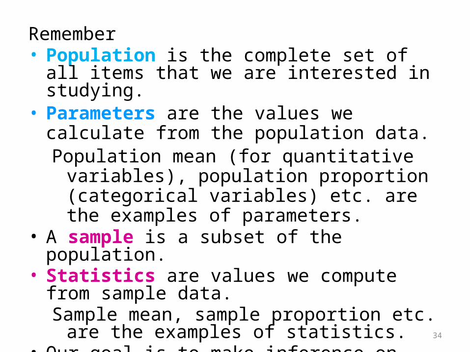
Remember• Population is the complete set of all items that we
are interested in studying.• Parameters are the values we calculate from the
population data.Population mean (for quantitative variables),
population proportion (categorical variables) etc. are the examples of parameters.
• A sample is a subset of the population.• Statistics are values we compute from sample data.
Sample mean, sample proportion etc. are the examples of statistics.
• Our goal is to make inference on parameters based on relevant statistics.
35
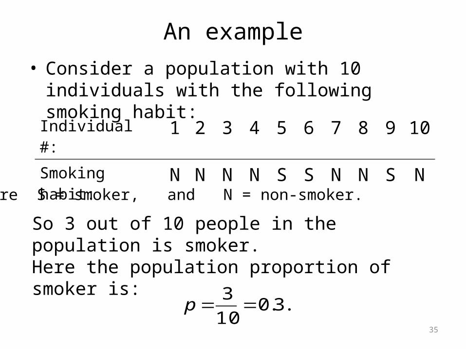
An example• Consider a population with 10 individuals with the
following smoking habit:
Individual #: 1 2 3 4 5 6 7 8 9 10
Smoking habit: N N N N S S N N S N
So 3 out of 10 people in the population is smoker.Here the population proportion of smoker is:
.3.010
3p
where S = smoker, and N = non-smoker.
36
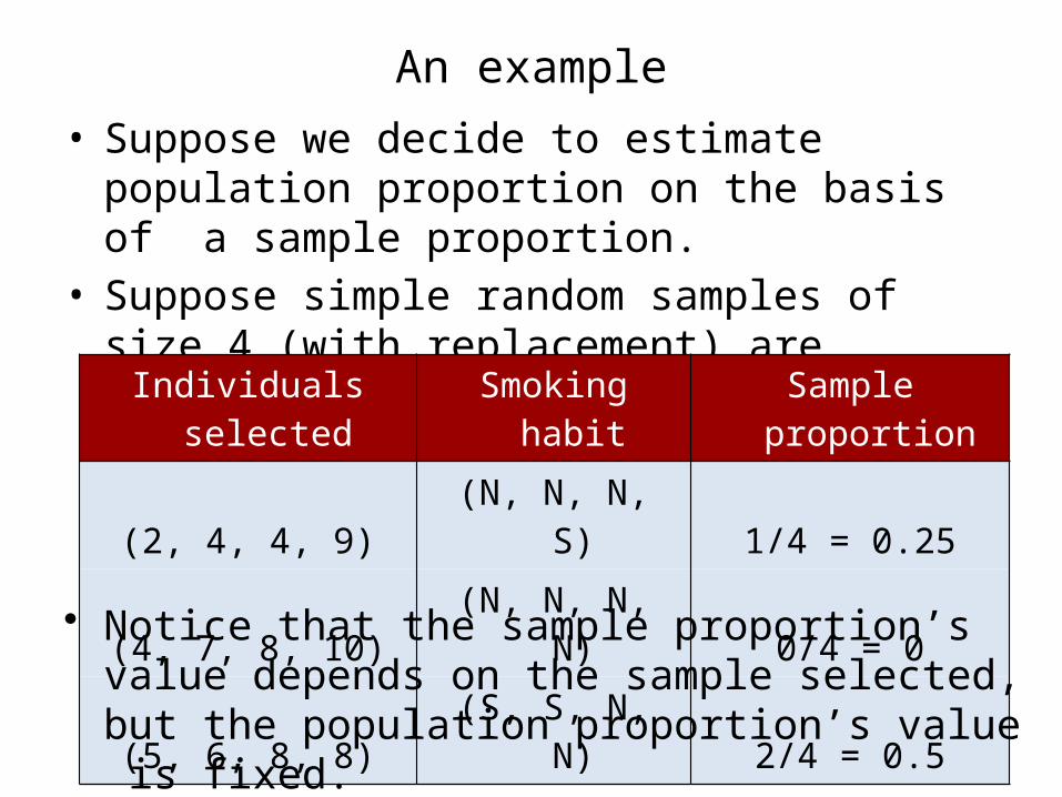
An example• Suppose we decide to estimate population
proportion on the basis of a sample proportion.• Suppose simple random samples of size 4 (with
replacement) are considered.
Individuals selected Smoking habit Sample proportion
(2, 4, 4, 9) (N, N, N, S) 1/4 = 0.25
(4, 7, 8, 10) (N, N, N, N) 0/4 = 0
(5, 6, 8, 8) (S, S, N, N) 2/4 = 0.5
• Notice that the sample proportion’s value depends on the sample selected, but the population proportion’s value is fixed.
37
Few questions• Can we justify the use of sample proportion as an
estimator of population proportion?• What can we expect about the value of sample
proportion when population proportion (p) is 0.3? Does this behavior depend on the value of p?
• What is the “margin of error”, if we estimate p with sample proportion? (To be answered in a later lecture.)
• As sample proportion is a variable, what is its distribution?
38
Few questions• Does it matter how the sample is selected?• Does the sample size matter?• Is this a problem of population proportion only?
Or do we face it for other parameters also?This is a problem for all parameters, which are fixed
in value for a particular population.The value of any statistic changes with the sample
selected.
39
Sampling Distribution• As any statistic’s value changes with the
selected sample, so statistic is a itself a random variable.
• The probability distribution of a sample statistic is called the sampling distribution of the statistic.
• In this course we shall study sampling distributions of sample proportion and sample mean.
40
Sampling method and sample size• Samples must be independent.
Simple random sampling “with replacement” ensures independence.
Holds (approximately) also for “without replacement” sampling as long as the sample size is smaller than 10% of the population size.
• Sample size must be “large enough”. What is “large enough” depends on the statistic we are
considering, i.e. different rules of “large enough” for sample proportion
and sample mean. It is the “sample size” what is important, NOT what fraction
of population is sampled.
41
Sampling distribution ofsample proportion
42
Sampling distribution of sample proportion
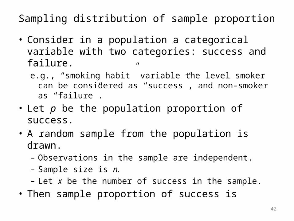
• Consider in a population a categorical variable with two categories: success and failure.e.g., “smoking habit” variable the level smoker can be
considered as “success”, and non-smoker as “failure”.
• Let p be the population proportion of success.• A random sample from the population is drawn.
– Observations in the sample are independent.– Sample size is n.– Let x be the number of success in the sample.
• Then sample proportion of success is
43
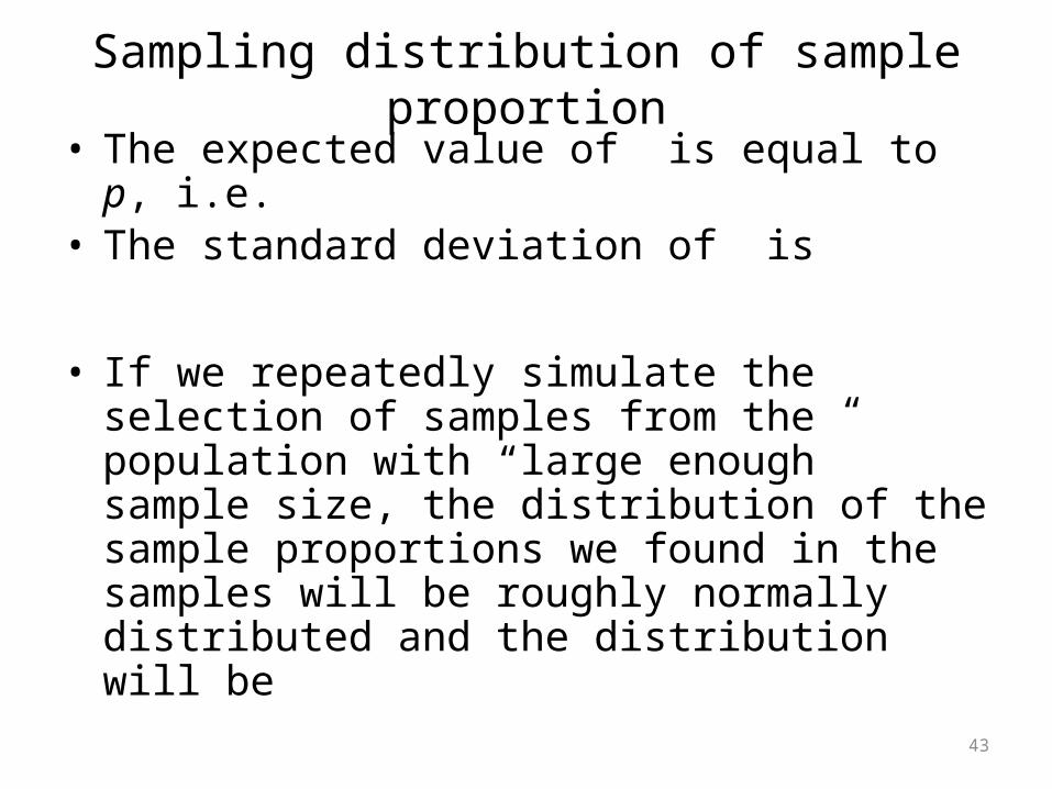
Sampling distribution of sample proportion• The expected value of is equal to p, i.e. • The standard deviation of is
• If we repeatedly simulate the selection of samples from the population with “large enough” sample size, the distribution of the sample proportions we found in the samples will be roughly normally distributed and the distribution will be
44
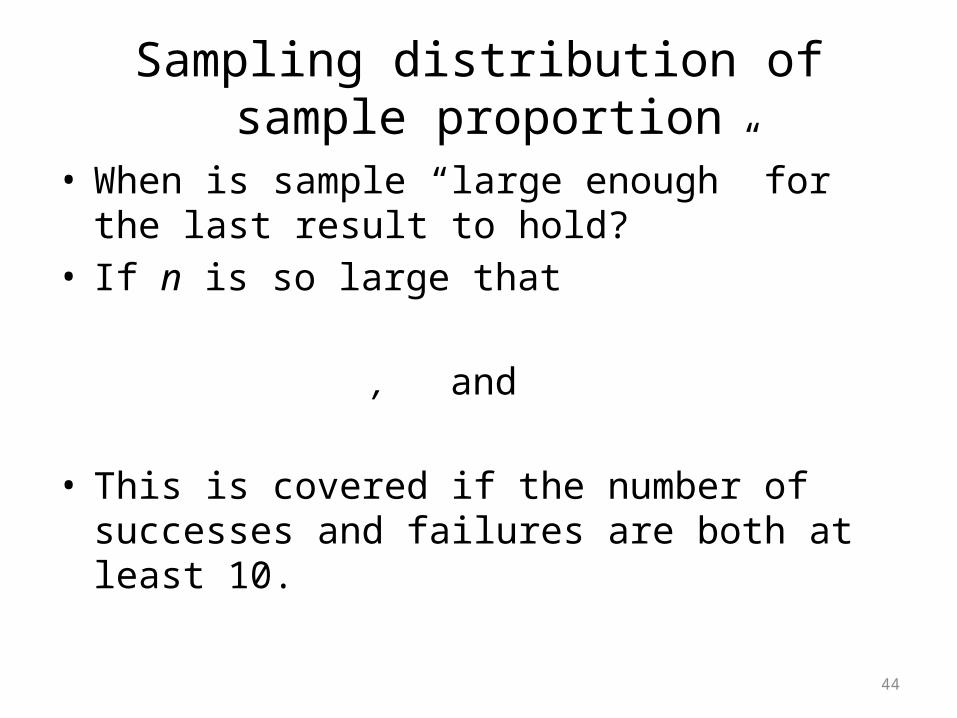
• When is sample “large enough” for the last result to hold?
• If n is so large that
, and
• This is covered if the number of successes and failures are both at least 10.
Sampling distribution of sample proportion

45
Example One
Is the independence condition met?Most likely NO, because the cars moving at the same
time may influence each others behavior.
Of all the cars on the highway, about 80% exceed the speed limit. If we clock the next 50 cars that pass, what might we expect to find?
Suppose we randomly select 50 cars that pass. Is the independence condition met?Yes.
46
Example One
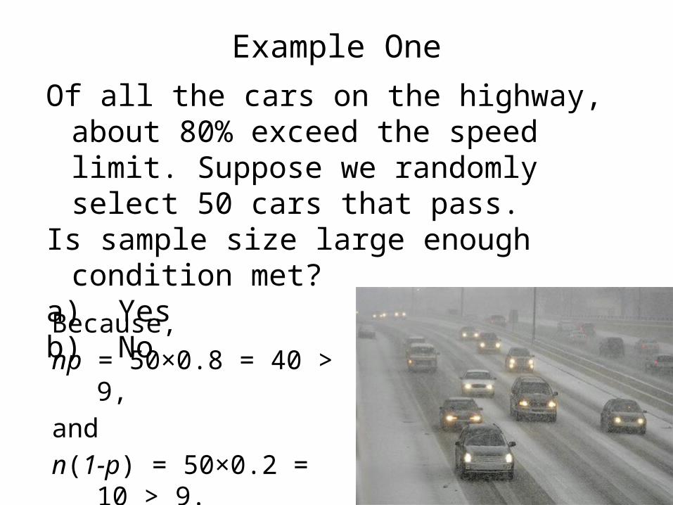
Because,np = 50×0.8 = 40 > 9,andn(1-p) = 50×0.2 = 10 > 9.
Of all the cars on the highway, about 80% exceed the speed limit. Suppose we randomly select 50 cars that pass.
Is sample size large enough condition met?a) Yesb) No
47
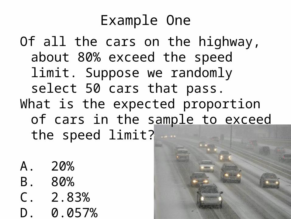
Example OneOf all the cars on the highway, about 80% exceed
the speed limit. Suppose we randomly select 50 cars that pass.
What is the expected proportion of cars in the sample to exceed the speed limit?
A. 20%B. 80%C. 2.83%D. 0.057%
48
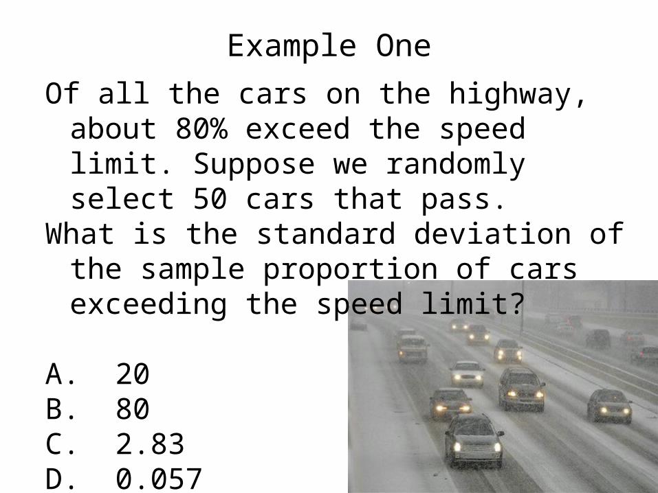
Example OneOf all the cars on the highway, about 80% exceed
the speed limit. Suppose we randomly select 50 cars that pass.
What is the standard deviation of the sample proportion of cars exceeding the speed limit?
A. 20B. 80C. 2.83D. 0.057
49
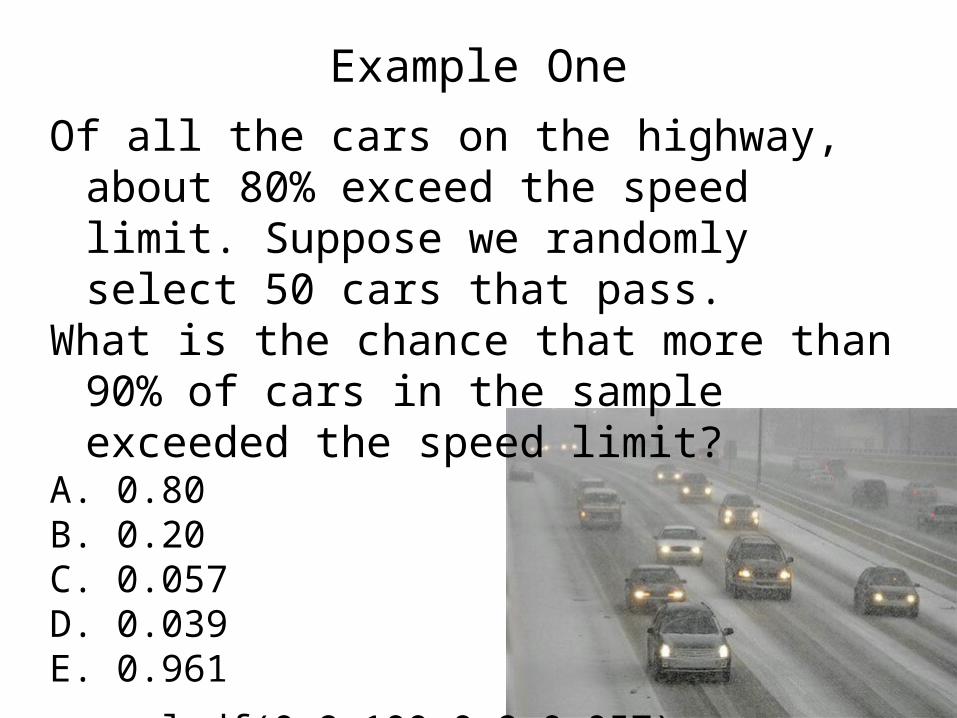
Example OneOf all the cars on the highway, about 80% exceed
the speed limit. Suppose we randomly select 50 cars that pass.
What is the chance that more than 90% of cars in the sample exceeded the speed limit?
A. 0.80B. 0.20C. 0.057D. 0.039E. 0.961
normalcdf(0.9,100,0.8,0.057)= 0.039.
50
Sampling distribution ofsample mean
51
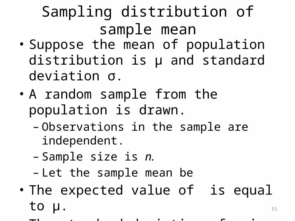
Sampling distribution of sample mean
• Suppose the mean of population distribution is µ and standard deviation σ.
• A random sample from the population is drawn.– Observations in the sample are independent.– Sample size is n.– Let the sample mean be
• The expected value of is equal to µ.• The standard deviation of is
52
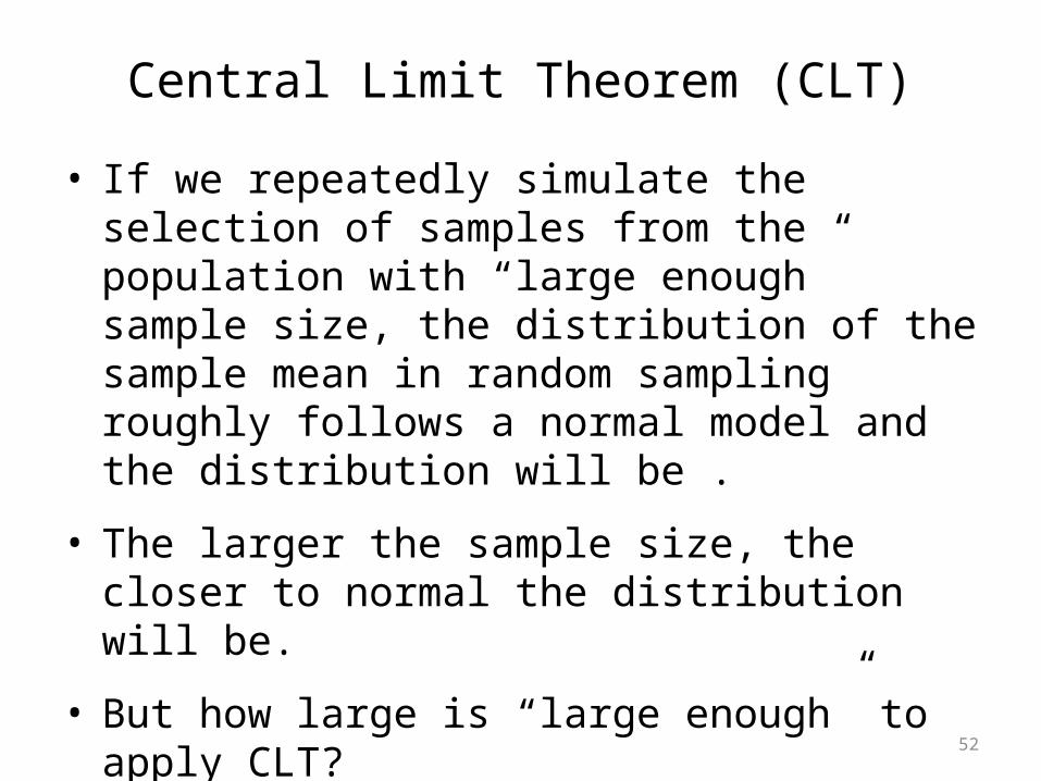
Central Limit Theorem (CLT)
• If we repeatedly simulate the selection of samples from the population with “large enough” sample size, the distribution of the sample mean in random sampling roughly follows a normal model and the distribution will be .
• The larger the sample size, the closer to normal the distribution will be.
• But how large is “large enough” to apply CLT?We can use CLT if
53
Example Two
What is the expected value of sample mean?A. 34 lbB. 7.2 lbC. 7.8 lbD. 2.1 lb
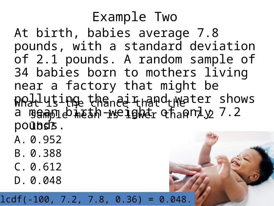
At birth, babies average 7.8 pounds, with a standard deviation of 2.1 pounds. A random sample of 34 babies born to mothers living near a factory that might be polluting the air and water shows a mean birth-weight of only 7.2 pounds.
54
Example Two
What is the standard deviation of sample mean?A. 1.23 lbB. 7.2 lbC. 0.36 lbD. 2.1 lb
At birth, babies average 7.8 pounds, with a standard deviation of 2.1 pounds. A random sample of 34 babies born to mothers living near a factory that might be polluting the air and water shows a mean birth-weight of only 7.2 pounds.
55
Example Two
What is the chance that the sample mean is lower than 7.2 lbs?
A. 0.952B. 0.388C. 0.612D. 0.048
At birth, babies average 7.8 pounds, with a standard deviation of 2.1 pounds. A random sample of 34 babies born to mothers living near a factory that might be polluting the air and water shows a mean birth-weight of only 7.2 pounds.
normalcdf(-100, 7.2, 7.8, 0.36) = 0.048.
56
ExampleIf price of gas (X) in East Lansing has uniform distribution in the interval $[3.45, 3.95] per gallon.Remember that Suppose we collect gas prices from 35 gas stations of East Lansing.• The expected sample average of gas prices is • The standard deviation of sample average of gas prices is • Since , we have • The chance that the sample average will be less than $3.65 is
57
ExampleIf the waiting time (X) for Bus #1 is exponentially distributed with mean 10 min. What is the chance that a sample average of 40 persons’ waiting time will be within 2 min of the mean time (10 min).• The expected sample average of waiting time is min.• The standard deviation of sample average of waiting
time is min.• Since , we have


![Mai 2016 [4.11 MB]](https://img.pdfslide.us/doc/110x75/5891b7ba1a28abc1698b6faf/mai-2016-411-mb.jpg)