Embed Size (px)
Citation preview

Strategic Investment Decisions for Product Development Projects -
An Option-Game Approach
by
Chung Lin Ku
A dissertation submitted to the Graduate Faculty of
Auburn University
in partial fulfillment of the
requirements for the Degree of
Doctor of Philosophy
Auburn, Alabama
May 9, 2015
Keywords: option-game, new product development, gate-criteria,
Bayesian analysis, Cournot competition, product differentiation
Copyright 2015 by Chung Lin Ku
Approved by
Chan Park, Chair, Daniel F. and Josephine Breeden Professor of Industrial Engineering
Jorge Valenzuela, Professor of Industrial Engineering
Ming Liao, Professor of Mathematics and Statistics

ii
Abstract
Gate-criteria have been identified as critical drivers of the success of a new
product development (NPD) process. However, a major weakness of NPD projects is
that gate-criteria are often inadequate for making go/kill decisions. The most commonly
used financial gate-criterion, the net present value (NPV) method, is insufficient when a
project involves uncertainty. Alternatively, the real-option valuation method is also
inadequate when a strategic decision involves the actions of competitors. In this research,
I first develop an option-game valuation framework that explicitly incorporates product
diffusion when dealing with an American investment option in a finite project life. The
results of both simultaneous and sequential investment decisions are considered in each
scenario of a duopolistic game. I introduce this approach as a gate-criterion to evaluate a
new product development project in a fast-paced industry while considering potential
managerial flexibility and market competition. As an option-game approach provides the
possibility of a go/wait decision, the decision to delay represents an additional resource of
value. Secondly, I further develop the option-game valuation framework with Bayesian
analysis by explicitly involving technical risk and the 3-player-game in an NPD project.
Volatilities from the initially uncertain market can be diminished as decision makers get
to know more about customer requirements and preferences, while uncertainties about
technical requirements are reduced through updated information about product
performance. In addition, the option-game mechanism includes (inverse) measures of

iii
product differentiation to describe whether two goods are homogeneous, substituted, or
independent, and to what degree. Moreover, the distribution of product correction is used
to describe the level of the additional correction costs in a project. I introduce this
approach as a gate-criterion to evaluate a new project at the gate and sub-gates of the
development stages in the NPD process. The results present important implications:
when demand is high, the project initiates “go” action if at least one competitor has a
high unit variable cost in competing with a highly comparable product or simply if the
target market is highly uncertain. When demand is low, the project may take “go” action
only if the firm has a cost advantage. By using these models, industry players can make
strategic decisions in a project assessment at the decision points of the development
stages.

iv
Acknowledgments
First and foremost, I would like to express my deepest appreciation to my
committee chair, Professor Chan Park, for his valuable guidance and advice. He showed
great patience and offered me a broad space and freedom in doing research. He inspired
me greatly to work in this research. I felt motivated and encouraged every time I
attended his meetings. Without his knowledge and assistance, this study would not have
materialized. I would also like to thank my committee members, Professor Jorge
Valenzuela and Professor Ming Liao, for providing me valuable information for guiding
this research. Special thanks to Ms. Sarah Johnson and Mr. Johnny Summerfield as both
my editors and proofreaders. Finally, yet importantly, I would like to express my
heartfelt thanks to my beloved parents and family for their understanding, blessings, and
endless love, and to all my friends/classmates/colleagues for their help and wishes for the
successful completion of this research. Especially, I wish to express my love and
gratitude to my beloved grandparents, who are always in my heart, for their constant
support and endless love. Most importantly, I am sincerely indebted to my beloved
husband, Mike Wang, for his understanding, endless patience, and encouragement when
it was most required. Without the support of the people mentioned above, this
dissertation would not have been possible.

v
Table of Contents
Abstract ………………………………………………………………………………... ii
Acknowledgments ……………………………………………………………………… iv
List of Tables …………………………………………………………………………… ix
List of Figures……………………………………………………………………………. x
Chapter 1 Introduction ……...…………………………………………………………… 1
1.1 Motivation and Research Issues …………………………………………… 1
1.2 Problem Statement ……………………………………….………………… 5
1.3 Research Objective ………………………………………………………… 9
Chapter 2 Literature Review…………………………………………………………..... 12
2.1 New Product Development ………………………………………………… 12
2.2 Real-Option Analysis …………………………………….………………… 16
2.2.1 Common real-option ……………………………….………………… 17
2.2.2 Basic option valuation …………………………….………………… 18
2.2.3 The real-option approach in NPD projects …………...……………… 20
2.3 The Option-Game Approach …………….……………….………………… 21
2.3.1 An illustration of the option-game approach ...…….………………… 22
2.3.2 Applications ………….…………………………….………………… 24
2.4 Decision Models with Information Updating …………....………………… 25
2.4.1 Information generation and updating ………..…….………………… 26

vi
2.4.2 Basic ideas of Bayesian analysis ………….……….………………… 27
2.4.3 The real-option approach with information updating ...……………… 27
2.5 Summary of the Literature ……………………………....………………… 29
Chapter 3 Assessing Investment Flexibility in a New Product Development Project:
An Option-Game Approach with Product Diffusion ….…………………..... 31
3.1 Background ………………………………………………………………… 32
3.1.1 Issues in the new product development ……………....……………… 32
3.1.2 The go/kill gate-criteria in the NPD process ……………....………… 34
3.1.3 The scope of this chapter ……………....…………………………….. 35
3.2 Model Development ……………....………………………………………... 38
3.2.1 Demand evolution and the probabilities of upward in demand with
product diffusion ……....…………………………………………….. 41
3.2.2 Payoff matrix of option-game at time t = 0 ………………………….. 43
3.2.3 Strategic decisions and the planned capacity …………….…….……. 53
3.2.4 Benchmark: the NPV approach ………………...……………………. 54
3.3 Case Study ………………...……………………………………………….. 55
3.3.1 Demand structure patterns with product diffusion …………………... 57
3.3.2 Strategic decisions and the optimal planned capacity ……………….. 59
3.3.3 Sensitivity analyses ………………………………………………….. 61
3.3.4 Interpretation of the results …………………………………………... 61
3.4 Validation and Discussion ……………………………………………….. 62
3.4.1 Validation ……………………………………………………………. 62
3.4.2 Limitations and possible extensions …………………………………. 68
3.5 Summary and Conclusion ………………………………………………….. 69

vii
Chapter 4 Assessing Managerial Flexibility in a New Product Development Project:
An Option-Game Approach in a Duopoly with Bayesian Analysis ………… 71
4.1 Background ………………………………………………………………… 72
4.1.1 New product development (NPD) …………………………………… 72
4.1.2 Problem statement …………………………………………………… 73
4.1.3 The scope of this chapter …………………………………………….. 75
4.2 Model Development ………………………………………………………... 78
4.2.1 Demand evolution and the probabilities of upward in demand ……… 81
4.2.2 Demand variance update: Bayesian analysis ………………………… 87
4.2.3 Discrete option-game valuation ……………………………………… 90
4.3 Case Study …………………………………………………………………. 93
4.3.1 Strategic decisions at the starting point (the gate of
go-to-development)……………………………………………………96
4.3.2 Strategic decisions at the sub-gates with Bayesian analysis ………… 96
4.3.3 Interpretation of the results …………………………………………. 100
4.4 Validation and Discussion …………………………………………….… 102
4.4.1 Validation …………………………………………………………. 102
4.4.2 Discussion ………………………………………………………….. 110
4.5 Summary and Conclusion ………………………………………………… 120
Chapter 5 Assessing Managerial Flexibility in a New Product Development Project:
An Option-Game Approach in an Oligopoly with Bayesian Analysis ……. 123
5.1 Background ……………………………………………………………….. 124
5.1.1 Problem statement ………………………………………………….. 124
5.1.2 The scope of this chapter …………………………………………… 125
5.2 Model Development ………………………………………………………. 127

viii
5.2.1 Demand evolution and the probabilities of upward in demand …….. 129
5.2.2 Demand mean and variance update: Bayesian analysis ……………. 136
5.2.3 Discrete option-game valuation …………………………………….. 141
5.3 Case Study ………………………………………………………………... 145
5.3.1 Strategic decisions at the starting point (the gate of
go-to-development) ……………...…………………………………. 148
5.3.2 Strategic decisions at the sub-gates with Bayesian analysis ……….. 149
5.3.3 Interpretation of the results …………………………………………. 156
5.4 Model Properties ………………………………………………………….. 158
5.4.1 Strategic decisions at the first sub-gate of development …………… 159
5.4.2 Limitations and possible extensions ………………………………... 164
5.5 Summary and Conclusion ………………………………………………… 165
Chapter 6 Summary and Conclusions ……………………………………………… 168
References ……………………………………………………………………………. 172
Appendix A Strategic Outcomes and Derivation of Equations……………...……… 184
Appendix B Case Study ………..…………………………………………………… 200
Appendix C Validation ……………………………………………………………… 219

ix
List of Tables
Table 2.1 Common real-option ………………………………………………………… 19
Table 3.1 Payoff matrix at time t = 0 …………………………………………………... 60
Table 3.2 The optimal planned capacity ……………………………………………….. 60
Table 4.1 The current payoffs at starting point of Firm i by benchmark A and my
approach ……...……………………………………………………………… 96
Table 4.2 Parameters of the prior distribution of customer requirements and
preferences ………………………………………………………………….. 97
Table 4.3 Parameters of posterior distribution of customer requirements and
preferences ………………………………………………………………….. 97
Table 4.4 The SNPVs (at the first sub-gate) by benchmark B and my model after
Bayesian analysis ………………………………………………………… 100
Table 5.1 Current payoffs (gate of go-to-development) of Firm i by benchmark A
and my model …………………………………………….……………..… 149
Table 5.2 Estimated moments of prior distribution of customer requirements and
preferences ……………………………………………………….………… 150
Table 5.3 Parameters of prior distribution of product performance ………………….. 151
Table 5.4 Parameters of posterior distribution of product performance ……………… 152
Table 5.5 The SNPVs (first sub-gate of development) of Firm i by benchmark B
and my approach after Bayesian analysis ………………………………… 154
Table 5.6 Strategic decisions at the status of “11” of Firm i when σ = 0.25, 0.45,
and 0.75 …………………………………………………………………… 160
Table 5.7 Strategic decisions at the status of “10” of Firm i when σ = 0.25, 0.45,
and 0.75 ………………………………………………………………...…. 161

x
List of Figures
Figure 1.1 Product management: primary role influencers …………………………….. 4
Figure 1.2 Problem definitions ………………………….………………………………. 6
Figure 1.3 Schematic diagram of research ……………………………………………. 10
Figure 2.1 Financial options versus real-option methods ……………………………… 18
Figure 2.2 Binomial tree representing evolution of market uncertainty and
associated probabilities …………….………………………..……………. 23
Figure 2.3 Structure of an option-game involving both market (demand) and
strategic (rival) uncertainty ……………….……………………………….. 24
Figure 2.4 Summary of the literature ………………………….……………………….. 30
Figure 3.1 The strategic buckets approach in the NPD process ……………………….. 36
Figure 3.2 The structure of model development ……………………………………….. 39
Figure 3.3 Multiplicative binomial process followed by the intercept of demand at time t ………………………….………………………………………….. 44
Figure 3.4 Payoff matrix for strategic decision at time t = 0 …………………………... 45
Figure 3.5 Payoff matrix for strategic investment decision at time t = 2 ……………… 50
Figure 3.6 Payoff matrix for strategic investment decision at time t = 1 ……………… 51
Figure 3.7 Profit maximization for each strategic investment decision at time t = 0 ….. 54
Figure 3.8 The binomial lattice with product diffusion of N = 4 product life cycle …… 58
Figure 3.9 Demand distribution at T = 2 (The first demand structure pattern:
if either firm invests now) ………………………….……………………... 59
Figure 3.10 Investment decisions and payoffs at maturity in an asymmetric Cournot
duopoly ………………………….………………………………………… 63

xi
Figure 3.11 Sensitivity analysis of option premium by changing the expected
standard deviation of demand σ ………………………….………………. 65
Figure 3.12 Sensitivity analysis of option premium by changing the expected yearly
growth rate g ………………………….…………………………..…….... 66
Figure 3.13 Sensitivity analysis of option premium by changing the ratio of firms’
unit costs βvc ………………………….……………………………………. 66
Figure 3.14 Sensitivity analysis of option premium by changing the annual reduced
rate of the fixed investment cost λ ……………………………………….. 67
Figure 4.1 Decision-making during the stages of product development ………………. 76
Figure 4.2 Product development process and the corresponding cash flows ………….. 79
Figure 4.3 The concept of model structure …………………………………………….. 80
Figure 4.4 Demand binomial lattice and the decision gate and sub-gates ……………... 82
Figure 4.5 Multiplicative binomial process followed by the intercept of demand at time t ………………………….………………………………………….. 84
Figure 4.6 Cash flows in this numerical example ……………………………………… 95
Figure 4.7 Prior and posterior distributions of customer of requirements and
preferences x ………………………….…………………………………… 98
Figure 4.8 Prior and posterior distributions of demand at product launch point Q1
(at year 1) ………………………….………………………………………... 99
Figure 4.9 Sensitivity analysis of SNPV of OG (option-game), NPV (benchmark A),
and OP (option premium) of Firm i by changing the expected standard
deviation in demand σ ………………………….………………………... 103
Figure 4.10 Sensitivity analysis of SNPV of OG (option-game), NPV (benchmark A),
and OP (option premium) of Firm i by changing a parameter of the
(inverse) product differentiation τ ……………….……………………….. 104
Figure 4.11 Sensitivity analysis of SNPV of OG (the option-game approach), NPV
(benchmark A), and OP (option premium) of Firm i by changing the ratio
of unit costs βvc ………………………….………………..……………. 105
Figure 4.12 Sensitivity analysis of SNPVs of Firm i by changing the expected
standard deviation in demand σ ………………………….……………… 107

xii
Figure 4.13 Sensitivity analysis of SNPVs of Firm i by changing the parameter of
the (inverse) product differentiation τ …………………………………... 108
Figure 4.14 Sensitivity analysis of SNPVs of Firm i by changing the ratio of
unit costs βvc ………………………….…………………………….……. 109
Figure 4.15 Strategic decisions of Firm i with low expected standard deviation
in demand σ ………………………….…………………………………… 111
Figure 4.16 Strategic decisions of Firm i with medium expected standard deviation
in demand σ ………………………….…………………………………… 112
Figure 4.17 Strategic decisions of Firm i with high expected standard deviation
in demand σ ………………………….…………………………………… 112
Figure 4.18 Maximum value of information (VImax
) at status “11” of Firm i by
changing the expected standard deviation in demand σ’ ………………… 115
Figure 4.19 Sensitivity analysis of the profits in the market by changing the ratio
of unit costs βvc (τ = 0.9) ……………………….………………………… 116
Figure 4.20 Downward-sloping reaction functions in an asymmetric Cournot
quantity competition ………………………….………………………….. 118
Figure 4.21 Sensitivity analysis of reaction functions by changing the (inverse)
product differentiation τ ………………………….………………………. 119
Figure 5.1 Product development process and the corresponding cash flows
(from Fig. 4.2) ………………………….…………………………………. 129
Figure 5.2 Demand binomial lattice and decision gate and sub-gates (from Fig. 4.4) .. 130
Figure 5.3 Multiplicative binomial process followed by the intercept of demand at time t ( 4t ) (from Fig. 4.5) ……………………………………………
1 3 2
Figure 5.4 Cash flows in this numerical example (from Fig. 4.6) ……………………. 147
Figure 5.5 The strategic decisions of Firm i in the distribution of product correction
at time 0 ………………………….………………………………………... 149
Figure 5.6 Prior and posterior of customer requirements and preferences x …………. 151
Figure 5.7 Prior and posterior of product performance s ……………………………... 152

xiii
Figure 5.8 Prior and posterior of demand at product launch phase Q1 (at time 1) ……. 153
Figure 5.9 The strategic decisions of Firm i in the distribution of product correction
at the status of “11” ………………………….……………………………. 155
Figure 5.10 The strategic decisions of Firm i in the distribution of product correction
at the status of “10” ………………………….…………………………… 156
Figure 5.11 The SNPVs from Table 5.6 when σ is low (σ = 0.25) …………………… 162
Figure 5.12 Strategic decisions at the status of “11” of Firm i when σ is low ………. 163
Figure 5.13 Strategic decisions at the status of “11” of Firm i when σ is medium …… 163
Figure 5.14 Strategic decisions at the status of “11” of Firm i when σ is high ……….. 163
Figure 5.15 Strategic decisions at the status of “10” of Firm i when σ = 0.25, 0.45,
or 0.75 ………………………….………………………………………… 164

1
Chapter 1 Introduction
1.1 Motivation and Research Issues
The project selection and portfolio choices that managers make are one of the most
critical decisions in any business. Academic and industry participants rank new product
project selection as one of the key issues in the new product development (NPD) process
of high-tech companies (Scott, 2000).
However, the majority of businesses surveyed in Cooper and Edgett’s study (2012)
indicated that they lacked a fact-based and objective approach to decision-making at their
gates of the NPD process. For example, before Microsoft agreed to acquire the handset
and services business of Nokia in 2013, Nokia's global market share had been in a
meltdown since 2009 (Steinbock, 2013). Analysts pointed out that Nokia's failure mainly
resulted from its lack of response in growth and flexibility in the US and emerging
markets (Steinbock, 2013). In addition, in 2012, three of Japan’s consumer electronics
giants (Sony, Sharp, and Panasonic) showed significant losses "from huge investments in
the wrong technologies to a reluctance to exit loss-making businesses" (Tabuchi, 2012).
Moreover, Cooper (2008) further mentioned that there are “too many projects in the
pipeline” in the NPD process. Accordingly, my research has been motivated by the need
for more effective criteria for product selection decisions.
Companies have recognized that the choice of products in their portfolios is a
central factor influencing their chance of success (Miguel, 2008; Cooper et al., 1997).

2
Therefore, portfolio management for new product and R&D spending has gained
tremendous attention over the decades (Miguel, 2008; Cooper et al., 1997, 2001; Scott,
2000). Portfolio management is defined as a process in which projects for new product
development, including both potential new projects and existing projects, are continually
evaluated, selected and prioritized (Cooper et al., 1997). As NPD is widely regarded as a
vital source of competitive advantage (Bessant & Francis, 1997), the product
development process from idea to launch consists of multiple phases, such as the project
screening, monitoring, and progression frameworks of Cooper’s stage-gate approach, in
which a stage-gate process is a conceptual and operational blueprint for managing an
NPD process (Cooper, 2008).
Since it is important that the selected projects are consistent with a business’s
strategy (Cooper et al., 1997), both academic and industry experts rank strategic planning
for technology products as the top issue for NPD project success (Scott, 2000). In order
to firmly link project selection and R&D spending to a business’s strategy, one strategic
technique is the strategic buckets method (Cooper et al., 1997). In this method, projects
are classified into “buckets” and then project candidates within each bucket are rank-
ordered by scoring models or financial criteria. The active projects within each bucket
are prioritized based on limited allocated resources, then moved to the next stage for
further investigation. The individual projects proceed to the subsequent development
process on an ongoing basis through the stage-gate process. In this process, each stage of
development is preceded by a “gate.” At each gate, go/kill decisions are made to manage
the risks of new products and to serve as quality-control checkpoints to continue moving

3
the right projects forward (Cooper & Edgett, 2012; Cooper, 2008; Carbonell-Foulquié et
al., 2004).
Effective portfolio decisions for NPD projects are a major challenge if the
organization is to stay in business. To help companies make effective decisions about
project selection, practitioners and researchers have proposed many mathematical
approaches such as mathematical programming models, net present value (NPV), scoring
models, and multi-attribute approaches. Due to the mathematical complexity of these
models, only a few are actually being used (Meade & Presley, 2002). Of the various
portfolio management methods, the ones most commonly used in R&D project selection
are the financial criteria methods such as NPV and internal rate of return (IRR) (Meade &
Presley, 2002). According to IRI’s collected questionnaires (Cooper et al., 2001), a total
of 40.4 percent of businesses rely on financial criteria as their dominant portfolio method,
yet those businesses end up with the worst and poorest performing portfolios. The main
reason for the poor performance of financial criteria methods is that prioritization
decisions are made in the early stages of a project when the financial data are least
accurate (Cooper et al., 2001).
In order to gain detailed insight into NPD projects, a method for strategic decision-
making primarily needs to measure and define the performance of the NPD. As most
firms’ ultimate objective is financial success (Griffin & Page, 1996), the standard
financial analysis methods for NPD projects are either the return on investment (ROI)
method or the net present value (NPV) method (Ulrich & Eppinger, 2004; Speirs, 2008).
The former, which evaluates the efficiency of the investment, is calculated as the return
of an investment divided by the cost of the investment. The latter, which measures the

4
present value of the project, is converted from the expected net cash flow from each
period estimated from various variables, as shown in Fig. 1.1. The primary role
influencers for this method are R&D, production, customers, marketing research, sales,
and advertising.
Managers make strategic decisions according to the innovativeness of the product,
market targeting, the number of competitors, and the marketability of the product
(Hultink et al., 1997). Across a firm’s total set of product development projects, success
needs to be measured and achieved for each of the independent multidimensional product
development outcomes, including consumer-based success, financial success, and
technical or process-based success (Griffin & Page, 1996; Craig & Hart, 1992; Griffin &
Page, 1993; Hart, 1993). Accordingly, the primary role factors and influencers in product
management (Fig. 1.1) need to be considered in an interrelated manner.
Fig. 1.1 Product management: primary role influencers (Gorchels, 2000)

5
However, in the increasing demand for better products launched more frequently
and aimed at ever-narrowed customer segments (Holman et al., 2003), the standard NPV
method for strategic decision-making in NPD projects fails not only to capture
managerial flexibility (Harper, 2011), but also to consider new information about the
markets and the actions of competitors. To resolve the above issues, this study proposes
a promising quantitative integrated framework for decision-making.
1.2 Problem Statement
Go/kill criteria are the heart of project selection decisions because they determine
whether a development project is allowed to continue through the development process
(Carbonell et al., 2004). A wrong decision can lead to wasted resources and losses of
strategic and market position (Meade & Presley, 2002). Despite the significance of
go/kill criteria, the question of how to use them effectively is an area that has not yet been
addressed sufficiently. In particular, financial criteria are rarely used to evaluate new
products at the beginning of the NPD process (e.g., the idea screening and concept test
stages) because the projected financial data at the early stages of a project are limited and
inaccurate (Hart et al., 2003; Carbonell et al., 2004). Accordingly, the go/kill criteria for
the NPD process are critical features. However, in Cooper’s study (1995), the
management of many of the participating companies admitted that they had no criteria for
making the go/kill decision in their new product process. The formal gate-criteria that
are used most often are scoring methods and conventional financial measures such as
NPV, IRR, or ROI (Miguel, 2008; Carbonell et al., 2004; Cooper et al., 2001). Yet those
conventional financial methods give inadequate measurements when projects are
accompanied by risk and uncertainty (Meade & Presley, 2002; Scott, 2000; Sommer &

6
Loch, 2004). As a result, there is no comprehensive, cohesive, and rational alternative to
traditional financial techniques for businesses that are faced specifically with products
that have a rapidly changing, shorter life cycle or with new product projects that are
competitive and risky.
The standard financial analysis measures (e.g., NPV) for NPD projects fail to
account for all the opportunities and situations in a fast-changing environment.
Specifically, these methods suffer from three main problems that are summarized in Fig.
1.2 and stated as follows.
Fig. 1.2 Problem definitions
The NPV method cannot capture managerial flexibility in strategic decision-
making at the gates in the NPD process.
In the current marketplace, products are launched more frequently than in the past
and are aimed at ever-narrower customer segments (Holman et al., 2003). Therefore, it is
important for businesses to have the managerial flexibility (Holman et al., 2003) and the

7
speed (McDaniel & Kolari, 1987; Miles et al., 1978) to change their products and
markets in response to changing environmental conditions.
The NPV method does not consider new information about the targeted
market and the actions of competitors.
The standard NPV method for strategic decisions in NPD projects fails not only to
capture managerial flexibility, but also to consider new information related to markets
and competitors. In the traditional real-option framework, the new information is
subjectively included in the analysis; however, methods for incorporating the arrival of
new information into an option’s value are still underdeveloped (Artmann, 2009;
Sundaresan, 2000; Martzoukos & Trigeorgis, 2001; Herath & Park, 2001; Miller & Park,
2005). While voice-of-the-customer input has been identified as one of the drivers of
success in the NPD process (Cooper & Edgett, 2012; Calantone et al., 1995), the major
project selection criteria should involve developing an understanding of customer
requirements (Scott, 2000; Bessant & Francis, 1997; Griffin & Hauser, 1996).
In addition, because “similar product developments exist in greater or lesser degree
in almost all product areas” (Smith, 1995), the competitor's involvement in a dynamic
setting could influence one firm’s output choice in the target market. Hence, in the
competitive marketplace, the real-option valuation methods fall short in resolving the
dilemma when the moves of a rival are involved (Ferreira et al., 2009). Moreover, as the
project success needs to be measured and achieved in multiple dimensions (Griffin &
Page, 1996), the primary role influencers in product management need to be considered
in an interrelated manner. Hence, other concepts and methods that have been developed
for solving these problems, such as the game theory approach, might be applicable to new

8
product development and allow decision makers to integrate new or updated information
into product development projects.
NPD projects are rarely killed at gates after the idea screening (Jenner, 2007).
Without a practical valuation approach, firms in fast-paced industries are known for
rushing investments to pre-empt market shares (Smit & Trigeorgis, 2007). Fearing that
competitors’ growth will outpace their own, managers are too eager to invest excess cash
in new capacities (Ferreira et al., 2009; Faughnder, 2012; Carson, 2007). And while both
researchers and practitioners agree on the significance of gate-criteria (Carbonell-
Foulquié et al., 2004; Agan, 2010), gates are rated as one of the weakest areas in product
development (Cooper, 2008; Cooper, Edgett, & Kleinschmidt, 2002, 2005). Only 33
percent of firms have rigorous gates throughout the NPD process (Cooper, Edgett, &
Kleinschmidt, 2002, 2005). In too many companies, gates either do not exist or are not
effective, allowing numerous bad projects to proceed (Cooper, 2008; Jenner, 2007;
Cooper & Edgett, 2012). Therefore, a practical and quantitative framework is urgently
needed, especially in fast-paced industries.
The decision problem involves questions from two perspectives: questions about
project investment and managerial decisions and questions about collecting and
integrating new information. These questions include the following: What is the value of
flexibility in a product development project in response to the changing environmental
conditions of a competitor's moves and updated market information? How does Bayesian
analysis affect the project value and the strategic decisions? Should the current project
proceed to the next stage? How does this information impact a company’s investment
and managerial decisions?

9
1.3 Research Objective
The proposed problem in this research focuses on decision-making under market
uncertainty and intense competition in an NPD project. I intend to value managerial
flexibility, especially on the gate-criteria of individual project assessment and particularly
for the gates of development phase in the NPD process. Specifically, the objectives of
this research are:
To quantify an integrated framework and to provide a measure of and criteria
for product development performance considering the multiple dimensions of
product development.
To determine the investment and managerial decisions at the gate by valuing
flexibility in an NPD project in response to changing environmental
conditions of a competitor's moves and updated market information, while
maximizing the expected economic returns.
To assess updated information in a product development project and explore
how it impacts a company’s investment decisions and its competitive
advantages.
As illustrated in Fig. 1.3, three main issues have been proposed. Regarding primary
role influencers on strategic decisions in NPD projects, I will consider market demand
and moves of competitors. Annual market demand in a potential segmented market is
variable and may change during the initial NPD process. However, the uncertainty of
market demand can be reduced by acquiring additional information via deriving a general
Bayesian updating formulation during the development process to update initial forecasts

10
(Artmann, 2009). In addition, the actions of competitors could damage the value of the
product development projects before they enter the market. Therefore, the payoff matrix
of option-game is derived for the moves of a competitor in a comparable NPD project
and incorporated with a general Bayesian updating formulation of market demand
information.
In this approach, I present – to the best of my knowledge – the first decision model
for gate-criteria that integrates an option-game framework with statistical decision theory
in the form of Bayesian analysis in an NPD project.
Fig. 1.3 Schematic diagram of research
With the described model and analysis, this research contributes to developing the
decision models of the gate-criteria in the NPD process by deriving an option-game

11
framework with a method for updating information. It also provides a practical and
quantitative measure of product development performance from multidimensional
perspectives that will help product development teams make investment and managerial
decisions in NPD projects. Hence, this research further enhances the basis for decisions
for NPD projects in response to changing environmental conditions, managerial
flexibility, the competitor's moves, and updated market information.
The remainder of the dissertation is structured as follows: In chapter 2, I review the
relevant literature. Chapter 3 develops an option-game valuation framework that
explicitly incorporates a product life cycle (product diffusion) when dealing with an
American investment option in a finite project life. In addition, the results of both
potential simultaneous and sequential investment decisions are considered in each
scenario of a duopolistic game. I introduce this approach as a gate-criterion to evaluate a
new project in the NPD process with potential managerial flexibility and a competitor in
fast-paced industries. In chapter 4, I develop a discrete option-game valuation framework
that explicitly incorporates statistical decision theory in the form of Bayesian analysis. In
addition, I include an inverse measure of product differentiation in the option-game
mechanism to describe whether two goods are homogeneous, substituted, or independent,
and to what degree. I introduce this approach as the gate-criteria to evaluate a new
project at the gate and sub-gates of development stages in the NPD process. In chapter 5,
I extend the option-game valuation framework with Bayesian analysis that is developed
in chapter 4 by explicitly involving technical risk and 3-player-games in an NPD project.
Finally, chapter 6 summarizes the main findings and provides possible extensions of the
developed models for future research.

12
Chapter 2 Literature Review
For decades, practitioners and academics have studied the factors related to product
development success (Craig & Hart, 1992; Griffin, 1997; Griffin & Page, 1993, 1996;
Hart, 1993; Hart et al., 2003; McDaniel & Kolari, 1987). However, different strategies
produce different levels of dependence upon new product development (Griffin, 1997;
Griffin & Page, 1993, 1996; Hart, 1993). These differences mean that one set of
measures of overall success is unlikely to be suitable across firms with different strategies
(Griffin & Page, 1996). Instead of determining the factors of product development
success, in this research, I focus on assessing flexibility of an individual project in an
NPD process under changing environmental conditions.
This research framework is based on previously developed concepts which are not
comprehensively linked. To build this link between flexibility and its related system
attributes, the following literature review is split into four categories: new product
development, real-option analysis, the option-game approach, and decision models with
information updating.
2.1 New Product Development
New product development is widely regarded as a vital source of competitive
advantage (Bessant & Francis, 1997). A product development process from idea to
launch consists of multiple phases, such as the project screening, monitoring, and
progression frameworks of Cooper’s stage-gate approach, which is a conceptual and

13
operational blueprint for managing the NPD process (Cooper, 2008). Nowadays, instead
of a standardized mechanistic implementation process, there are many different versions
to fit different business needs (Cooper, 2008). In an idea-to-launch product process, each
stage has defined procedures and requires the gathering of relevant information.
Following each stage is a “gate” where go/kill decisions are made to manage the risks of
new products and to serve as a quality-control checkpoint to continue moving the right
projects forward (Cooper & Edgett, 2012; Cooper, 2008; Carbonell-Foulquié et al.,
2004).
In order to gain competitive advantages, companies must continuously introduce
successful and innovative products into the market (Holman, Kaas & Keeling, 2003;
Kaplan, 1954). However, the average success rate for NPD projects is not significantly
high (Griffin, 1997). Companies have recognized that the choice of products in their
portfolios is a central factor influencing their chance of success (Miguel, 2008; Cooper et
al., 1997). Therefore, portfolio management for new product and R&D spending has
gained tremendous attention over the decades (Miguel, 2008; Cooper et al., 1997, 2001;
Scott, 2000). Portfolio management is defined as a process in which projects for product
development, both new or potential projects and existing projects, are continually
evaluated, selected and prioritized (Cooper et al., 1997). Nevertheless, a benchmarking
study (Cooper et al., 1995) has identified portfolio management as the weakest area in
managing new product development.
Effective portfolio decision for NPD projects is thus a major challenge if the
organization is to stay in business. To help organizations make decisions about project
selection, practitioners and researchers have proposed many mathematical approaches

14
such as mathematical programming models, net present value (NPV), scoring models,
and multi-attribute approaches. However, due to the mathematical complexity of these
models, only a few are actually being used (Meade & Presley, 2002). Of various
portfolio management methods, the most commonly used in R&D project selection are
financial criteria (such as NPV and IRR) (Meade & Presley, 2002). Accordng to IRI’s
collected questionnaires (Cooper et al., 2001), a total of 40.4 percent of businesses rely
on financial criteria as their dominant portfolio method, but those businesses end up with
the worst and poorest performing portfolios. The main reason for the failure of financial
criteria is that prioritization decisions are made in the early stage of a project, when the
financial data are the least accurate (Cooper et al., 2001). In other words, the
conventional financial criteria do not succeed at predicting the future financial success of
a technology (Scott, 2000). As the initial NPD projects are risky and multidimensional in
nature, decisions about these projects should consider strategic and multidimensional
measures (Meade & Presley, 2002).
Moreover, both academic and industry experts have identified strategic planning for
technology products as a significant issue for NPD project success (Scott, 2000), since it
is important that the selected projects are consistent with a business’s strategy (Cooper et
al., 1997). A total of 26.6 percent of businesses use strategic approaches as the dominant
portfolio method, making them the second most popular portfolio approach (Cooper et
al., 2001). In order to firmly link project selection and R&D spending to a business’s
strategy, many companies use the strategic buckets method (Cooper et al., 1997). The
strategic bucket approach allocates spending to different buckets or envelopes based on
the business’s strategy and strategic priorities across various dimensions (e.g., type of

15
market, type of development, product line, and so on). After projects are classified into
buckets, project candidates within each bucket are rank-ordered by scoring models or
financial criteria. The active projects within each bucket are prioritized and allocated
limited resources, then moved to the next stage for further investigation. The individual
projects proceed to the subsequent development process on an ongoing basis through the
stage-gate process with the gate-criteria of go/kill decisions.
Go/kill criteria are the heart of project selection decisions, determining whether a
development project is allowed to continue through the development process (Carbonell
et al., 2004). A wrong decision can lead to wasted resources and losses of strategic and
market position (Meade & Presley, 2002). Despite the significance of go/kill criteria,
however, methods for using them successfully have not yet been addressed sufficiently.
In particular, financial criteria are rarely used to evaluate new products at the beginning
of the NPD process (e.g., the idea screening and concept test stages), because the
projected financial data in the early stages are limited and inaccurate (Hart et al., 2003;
Carbonell et al., 2004). Accordingly, go/kill criteria for the NPD process are critical
features. However, in Cooper et al.’s study (1995), the managers of many participating
companies admitted that they had no criteria for making the go/kill decision in their new
product processes. The formal gate-criteria that are used most often are scoring and
conventional financial measures such as the NPV, IRR, or ROI (Miguel, 2008; Carbonell
et al., 2004; Cooper et al., 2001). Yet those conventional financial methods give
inadequate measurements when projects are accompanied by risk and uncertainty (Meade
& Presley, 2002; Scott, 2000; Sommer & Loch, 2004).

16
Literature study has determined that the financial criteria for gate decisions after the
screening and investigation stages will positively impact new product success (Carbonell
et al., 2004; Hart et al., 2003). As different criteria can be used for projects from
different buckets, it is not necessary to develop a universal criterion that fits all projects
(Cooper et al., 1997). Nevertheless, the traditional valuation approach techniques, which
assume at the outset that all future outcomes are fixed, are used widely in business
(Krychowski & Quélin, 2010). The traditional valuation approach relies on a discounted
cash flow series, assuming that the investment is an all-or-nothing strategy in which the
net present worth or net present value (NPV) is considered as a project’s expected future
cash flow into the time value of money at time 0 with a risk-adjusted discount rate
(today’s dollars). The main problem with this approach is that it underestimates the
flexibility value of a project and assumes that all outcomes are static and all decisions
made are irrevocable (Mun, 2006). As a result, there is no comprehensive, cohesive, and
rational alternative to traditional financial techniques for businesses that are faced
specifically with rapidly changing, shorter product life cycles or competitive and risky
new product projects.
2.2 Real-Option Analysis
A real-option approach, building upon traditional discounted cash flow analysis,
gives decision makers a set of options without committing them to one particular
decision. The real-option approach considers flexibility in decision-making, and the
flexibility can be viewed as options or investment opportunities available to the company
(Antikarov et al., 2001). Therefore, the real-option approach allows managers to build
options into products and projects in the real world (Mun, 2006; Harper, 2011) and

17
increases the overall understanding of the investment decision, especially in areas of
uncertainty (Michailidis, 2006).
Cooper (2008) explains that the stage-gate process of an NPD project is very
similar to that of buying a series of options on an investment: as each stage of the
development process costs more than the preceding one, the initial amount of cost is
analogous to the purchase of an option, and the decision of whether or not to continue
investing in the project is made at the gate (maturity), while new information is gathered
during the stage. Indeed, the flexibility of the real-option approach corresponds to the
structure of the NPD process, allowing developers to build options into products and
projects (Mun, 2006). In the following sections, I provide a short introduction to the real-
option method and its applications in NPD projects.
2.2.1 Common real-option
Real-option theory originates from methodologies developed in the field of
financial analysis (Black & Scholes, 1973), but there are key differences between
financial options and real-option (Mun, 2006) as listed in Fig. 2.1. In addition,
management can benefit from different types of real-option, which are primarily
classified by sources of managerial flexibility, as shown in Table 2.1 (Smit & Trigeorgis,
2004; Chevalier-Roignant & Trigeorgis, 2011). In dynamic decision-making, the
manager’s actions depend on all information available at time 0 as well as all new
information revealed between times 0 and T (Guthrie, 2009). As a result, in a product
developer’s cost modeling, the value of future decisions can be explicitly incorporated
into calculations of expected returns from a project (Harper, 2011; Guthrie, 2009). In

18
other words, incorporating flexible options into the project plan can increase the financial
performance of the project over its entire life cycle (Harper, 2011).
Fig. 2.1 Financial options versus real-option methods (Mun, 2006)
2.2.2 Basic option valuation
Many numerical analysis techniques to value options take advantage of risk-neutral
valuation. In general, numerical techniques for option valuation can be classified into
two types (Smit & Trigeorgis, 2004):
Approximating the underlying stochastic processes: The first category includes
the Monte Carlo simulation used by Boyle (1977) and various lattice approaches,
such as Cox, Ross, and Rubinstein’s (1979) standard binomial lattice method and
Trigeorgis’s (1991) log-transformed binomial approach. These methods are

19
generally more intuitive, and the latter methods are particularly well suited to
valuing complex projects with multiple embedded real-option methods, a series of
investment outlays, dividend-like effects, and option interactions.
Approximating the resulting partial differential equations: Examples of the second
category include numerical integration and the implicit or explicit finite-
difference schemes used by Brennen (1979), Brennen and Schwartz (1978), and
Majd and Pindyck (1987).
Table 2.1 Common real-option (Chevalier-Roignant & Trigeorgis, 2011)
The two best-known option-pricing models are those of Black and Scholes (1973)
and Cox, Ross, and Rubinstein (1979). Originally, these models were designed to price
financial options, but they have been extended to valuing real-option models. The Black-

20
Scholes (BS) model involves advanced mathematics and notions of financial theory in
continuous time. The continuous-time models assume instantaneous decision-making
and are appealing because they help better identify the theoretical value drivers and
examine the underlying trade-offs. On the other hand, the discrete-time multiplicative
binomial model of Cox-Ross-Rubinstein (CRR) offers a more intuitive introduction to
option pricing. Discrete-time models are generally better suited to handling practical or
complex valuation problems (e.g., portfolios of real-option) and are easier to implement
(Chevalier-Roignant & Trigeorgis, 2011).
2.2.3 The real-option approach in NPD projects
The real-option approach has gained attention in the area of product development
projects (i.e., R&D project evaluation) since it can value managerial flexibility with
respect to contingent multi-stages in high-tech projects and the market uncertainty
inherent in the projects (Benninga & Tolkowsky, 2002; Loch & Bode‐Greuel, 2001;
Oriani & Sobrero, 2008; Huchzermeier & Loch, 2001; Santiago & Vakili, 2005).
Loch and Bode‐Greuel (2001) demonstrated a quantitative evaluation of compound
growth options in a large international pharmaceutical company using a decision tree to
provide transparency about project value and strategic options. Lint and Pennings (2001)
developed a real-option framework with market and technology uncertainty in a
development project. They also demonstrated how any particular project in the R&D
phase may be assigned within a 2 by 2 matrix of uncertainty versus R&D option value to
allow managers to decide whether to speed up or delay the development process. Oriani
and Sobrero (2008) provided new theoretical insights into the real-option logic and gave
empirical evidence of the effect of market and technological uncertainty on the market

21
valuation of a firm's R&D capital. Huchzermeier and Loch (2001) incorporated the
operational sources of uncertainty into real-option value of managerial flexibility and
introduced an improvement option to take corrective actions during the NPD process for
the purpose of better product performance. Santiago and Vakili (2005) used the practical
relevance of the improvement option to extend Huchzermeier and Loch’s (2001) work to
value a high-technology development project in the presence of technical uncertainties.
However, because “similar product developments exist in greater or lesser degree in
almost all product areas” (Smith, 1995), a competitor's involvement in a dynamic setting
could influence one firm’s output choice in the target market. Real-option theory mainly
considers single decision-maker problems which assume that firms are operating in a
monopoly or perfect competition markets (Huisman et al., 2004). These traditional
valuation methods fall short of resolving the dilemma when moves of competitors are
involved in the competitive marketplace (Ferreira et al., 2009). An additional problem
with these methods is the limited knowledge of how to evaluate projects and make
critical go/kill decisions throughout the entire development process (Schmidt &
Calantone, 1998; Carbonell-Foulquié, 2004).
2.3 The Option-Game Approach
The term “option-game” was developed by Smit and Trigeorgis (2006). Their
theory combines real-option (which relies on the evolution of prices and demand) and
game theory (which captures competitors’ moves) to quantify the value of flexibility and
commitment. As mentioned above, the traditional real-option valuations are inadequate
when moves of competitors are involved (Ferreira et al., 2009). Nevertheless, the real-
option approach has the potential to make a significant difference in the area of

22
competition and strategy. Many researchers have dealt with the concepts of competitive
and strategic options (Trigeorgis & Kasanen, 1991). Competitive investment strategy is
based on the strategic or expanded NPV criterion that incorporates not only the direct
cash-flow value and the flexibility or option value but also the strategic commitment
value from competitive interaction. The first two studies dealing with real-option context
in a duopoly were Smet’s (1991) and Dixit and Pindyck’s (1994). Their research has led
to a number of studies combining real-option and game theory (Smit & Trigeorgis, 2006)
in situations where several firms have the option to invest in the same project (Smet,
1991; Smit & Ankum, 1993; Smit & Trigeorgis, 1995; Chevalier-Roignant & Trigeorgis,
2011). In the following section, I provide a brief introduction to option-game and its
applications.
2.3.1 An illustration of the option-game approach
Chevalier-Roignant and Trigeorgis (2011) provided a simple illustration of the logic
behind option-game which is shown below. An option-game approach viewed in discrete
time is an overlay of a binomial tree onto a payoff matrix. A binomial tree (Fig. 2.2) is
used to model the stochastic evolution of project value (V), while two-by-two matrices
are used to capture the competitive iterations among players. In the binomial tree, each
scenario at the end of the node corresponds to the cumulative risk-neutral probability
after two steps, where qr is the risk-neutral probability of an upward per period.
Consider a duopoly consisting of Firms i and j sharing a European option to invest
in an emerging market within two years. Both firms can invest, wait and invest later (at
maturity in time 2), or let the option expire. If neither invests now, at the end node in
time 2, the firm’s strategic choices (represented in two-by-two payoff matrices) are either

23
to invest or not to invest (abandon). At maturity, both Firms i and j can invest, both can
abandon, or only one can invest (potentially involving a coordination problem). The
basic structure of this option-game in discrete-time is depicted in Fig. 2.3. Once the
binomial tree charts the evolution of potential demand scenarios until maturity (time 2) in
each end node, a two-by-two payoff matrix depicts the resulting competitive interaction.
The resulting equilibrium outcome (*) and corresponding player payoffs can be
anticipated for each of the three payoff matrices. Once the equilibrium (*) strategic
option values are obtained in each end state (C*++
, C*+-
, C*--), working the tree backward
enables the firm to assess the value that each strategy creates under rivalry. This analysis
reveals the benefits to each player of pursuing a given strategy and enables management
to determine how these benefits might change if certain key variables, such as growth or
volatility, change.
Fig. 2.2 Binomial tree representing evolution of market uncertainty and associated
probabilities (Chevalier-Roignant & Trigeorgis, 2011)

24
Fig. 2.3 Structure of an option-game approach involving both market (demand) and
strategic (rival) uncertainty (Chevalier-Roignant & Trigeorgis, 2011)
2.3.2 Applications
The real-option approach with a game theoretic concept has gained attention in the
area of strategic investment (Huisman, 2001; Egami, 2010; Beveridge & Joshi, 2011;
Huisman et al., 2004; Smit & Trigeorgis, 2007; Smit & Trigeorgis, 2009; Martzoukos &
Zacharias, 2012), since it can quantify the value of flexibility and commitment, allowing
decision makers to make rational choices (Ferreira et al., 2009).
Smit and Trigeorgis (2009) applied the option-game methodology to the case of
evaluating airport infrastructure expansion investments. They proposed important
advantages of a binomial-tree option-game, such as the transparency and tractability of
value movement dynamics; the modularity to embed strategic interactions, restrictions,

25
and other features in a realistic setting; and the intuitiveness and accessibility of the
methodological logic. Ferreira et al. (2009) illustrated that the option-game is suited for
competing in capital-intensive industries, using a simplified example of a mining
company considering whether or not to add new capacity in the face of demand and
competitive uncertainties, and analyzed four scenarios arising from their decisions to
invest now or wait. Martzoukos & Zacharias (2012) demonstrated to decision makers a
method for deciding on the best action strategy and the amount of effort in a competition
situation, a decision which is heavily dependent on the effectiveness of R&D
investments, their cost, and the degree of coordination that is optimal for the two firms.
However, with the increasing importance of customer orientation (Sun, 2006) in the
current fast-changing marketplace, if managers do not have updated information on
market requirements and foresight of market demand, this lack of information will
significantly affect strategic decisions as well as the sales of new products (Kahn, 2002;
Artmann, 2009).
2.4 Decision Models with Information Updating
Because voice-of-the-customer input has been identified as one of the drivers of
success in the NPD process (Cooper & Edgett, 2012; Calantone et al., 1995), the major
project selection criteria should involve developing an understanding of customer
requirements (Scott, 2000; Bessant & Francis, 1997; Griffin & Hauser, 1996). Due to
shorter product life cycles in fast-paced industries, it is not necessary to wait for perfect
information at the pre-defined gate for decision-making. Stages can be overlapped in a
stage-gate process by using spiral development, allowing product development to
continuously incorporate valuable customer feedback into the product design during the

26
NPD process until the final product is closer to customers’ ideal (Cooper, 2008). The
data obtained from customer feedback allows decision makers to estimate the potential
market share of each concept and to select an optimal product investment. Without
updated information on market requirements and foresight of market demand, the sales of
new products will be significantly affected (Kahn, 2002; Artmann, 2009). However, a
common problem is that companies collect data on customer interest before the start of
development activities and generally do not update the data (von Hippel, 1992; Artmann,
2009). Hence, problems arise if the customers’ needs change (Bhattacharya et al., 1998).
Researchers have developed numerous models for decision-making that allow managerial
flexibility for responding to new information in certain environments, permitting
management to refine its information over time and adjust its initial decisions (Artmann,
2009; Loch & Terwiesch, 2005).
2.4.1 Information generation and updating
Gathering high-quality data involves direct contact with customers and experience
with the use environment of the product. The most common means of generating market
information are the traditional market research methods (Lynn et al., 1999; Zahay et al.,
2004). Three methods are commonly used: interviews, focus groups, and observing the
product in use (Ulrich & Eppinger, 2004).
Depending on the issue being studied, the level of uncertainty about demand and
the methods for reducing uncertainty can be modeled in different approaches. There are
three major updating methods applied to decision models: time series analysis, Markov-
modulated forecast updates, and Bayesian analysis (Sethi et al., 2005).

27
2.4.2 Basic ideas of Bayesian analysis
Bayesian analysis is a statistical decision theory developed by Thomas Bayes
(1764). It is a popular method in the field of statistical decision theory, which is
concerned with the problem of making decisions based on statistical knowledge about
uncertain quantities. The decision maker’s challenge is to estimate an objective
probability model with critical parameters. Using statistical sample data from
experiments or market research about the unknown parameters, the Bayesian method
combines the sample data with initial information about the problem, allowing the
decision maker to obtain the posterior distribution of parameters. Hence, the objective
probability model can be updated. Because they are easily interpreted and suitable for
practical applications, the Bayesian methods have been used by researchers in various
disciplines and different applications over the last decade.
2.4.3 The real-option approach with information updating
In the traditional real-option framework, new information is subjectively included
in the analysis; however, methods incorporating the arrival of new information into an
option’s value are still underdeveloped (Sundaresan, 2000; De Weck et al., 2007;
Halpern, 2003; Martzoukos & Trigeorgis, 2001). Several researchers have observed the
traditional real-option framework and attempted to combine Bayesian analysis with real-
option (Herath & Park, 2001; Huchzermeier & Loch, 2001; Santiago & Vakili, 2005;
Miller & Park, 2005; Armstrong et al., 2005; Grenadier & Malenko, 2010) and Bayesian
learning with the binomial lattice model (Guidolin & Timmermann, 2003; Guidolin &
Timmermann, 2007).

28
Herath and Park (2001) were the first to introduce Bayesian analysis combined with
real-option. They developed a simple valuation framework based on the concept of the
expected value of perfect information (EVPI) of real-option and sampling information.
In their approach, they studied investment decisions where management has the option to
defer a project until more information becomes available. Miller and Park (2005)
indicated that reducing uncertainty in real-option theory has traditionally been regarded
as a passive process. In contrast, they quantified information acquisition by merging
statistical Bayesian perspective with the real-option framework to improve decision-
making and modeled a contingent multi-stage investment scenario in which the initial
estimates of the expected future cash flows are updated during the management phase of
the project. They identified a key threshold which defines when the firm’s prior decision
should be reversed based on observed sample results.
Armstrong et al. (2005) presented a primary practical application of a framework
that combines Bayesian analysis with a real-option approach. They studied the option
value of acquiring additional information in a project for enhancing oil field production.
They assumed that the two sources of uncertainty, the underlying oil prices and the
characteristics of the reservoir, were bivariate normal distribution by using a Monte Carlo
simulation. Grenadier and Malenko (2010) augmented the standard Brownian
uncertainty driving traditional real-option models with additional Bayesian uncertainty
over distinguishing between the temporary and permanent nature of past cash flow
shocks. Artmann (2009) derived the Bayesian updating formulation for an update of the
market requirement distribution that allows for managerial flexibility in a situation where
product performance is uncertain.

29
2.5 Summary of the Literature
A common problem with NPD processes is that projects are rarely killed at gates
after the stage of idea screening (Jenner, 2007). Additionally, Anderson (2008) pointed
out that the most significant challenge in managing current product development is the
overall integration of strategy, process, the measurement of performance, and continuous
improvement. As shown by the above review of the relevant literatures about flexibility
in NPD projects, the option-game approach, and decision models with information
updating, managers need a comprehensive quantitative model to improve decision-
making about the gate-criteria of NPD projects (Fig. 2.4). Cooper (2008) explained that
the stage-gate process of an NPD project is very similar to that of buying a series of
options on an investment. On the other hand, Huchzermeier and Loch (2001) proposed
an insightful framework of managerial flexibility in an NPD project, in which the
product’s developer considers an improvement option to take corrective actions during
the NPD process. In contrast to traditional real-option methods which regard uncertainty
reduction as a passive process (Miller & Park, 2005), Artmann (2009) extended the work
of Huchzermeier and Loch (2001) by deriving the Bayesian updating formulation for the
market requirement distribution and integrating this mechanism into a real-option
framework. Moreover, Chevalier-Roignant and Trigeorgis (2011) studied and illustrated
the option-game framework, which allows decision makers to make rational choices
between alternative investment strategies (Ferreira et al., 2009), combining real-option
models (which rely on the evolution of prices and demand) and game theory (which
captures competitors’ moves).

30
The above four areas make the option-game framework well suited for NPD
projects as well as for a base case demonstrating the decision models of the gate-criteria
with information updating under competitive environments. The current option-game
models are not considered Bayesian learning analysis. Therefore, I introduce an option-
game valuation framework with Bayesian analysis as a gate-criterion of a new project in
the NPD process. By gathering new information about potential markets, project payoff,
and the rivals’ actions, a decision maker can use this integrated approach to make the
proper strategic decisions in the NPD process.
Fig. 2.4 Summary of the literature

31
Chapter 3 Assessing Investment Flexibility in a New Product
Development Project: An Option-Game Approach
with Product Diffusion
Abstract
Project selection of new products is a vital issue in the new product development
(NPD) process of high-tech companies. A major problem with project selection is the
inadequacy of using gate-criteria to make the go/kill decisions. The most common
financial gate-criterion, the net present value (NPV), is insufficient when a project has a
high degree of uncertainty, resulting in killing potential projects unnecessarily. In this
chapter, I develop an option-game valuation framework that explicitly incorporates
product diffusion when dealing with an American investment option in a finite project
life. In addition, the results of both potential simultaneous and sequential investment
decisions are considered in each scenario of the duopolistic game. I introduce this
approach as the gate-criterion to evaluate a new project in the NPD process with potential
managerial flexibility and a competitor in fast-paced industries. As an option-game
approach provides a go/wait decision, it shows that the decision to delay represents an
additional resource of value. The results provide important implications for strategic
project selection when investigating an NPD project during the product development
process. By using this approach, industry players can make strategic decisions in a

32
project assessment and plan the optimal annual production capacity at the outset of the
product development stage.
Keywords: option-game, product diffusion, gate-criteria, new product
development, Cournot duopoly competition, sequential investment
3.1 Background
According to Scott (2000), academic and industry participants rank new product
selection as one of the most critical issues in the NPD process of high-tech companies.
Indeed, the project selection and portfolio choices that managers make will guide
businesses’ new product efforts either toward or away from their organizational goals.
3.1.1 Issues in the new product development
In order to gain competitive advantages, companies must continually introduce
successful and innovative products into the market (Holman, Kaas, & Keeling, 2003;
Kaplan, 1954). However, the average success rate for NPD projects is not significantly
high (Griffin, 1997). Companies have recognized that the choice of products in their
portfolios is a central factor influencing their chance of success (Miguel, 2008; Cooper et
al., 1997). Therefore, portfolio management for new product and R&D spending has
gained tremendous attention over the decades (Miguel, 2008; Cooper et al., 1997, 2001;
Scott, 2000). Portfolio management is defined as a process in which projects for product
development, both new or potential projects and existing projects, are continually
evaluated, selected and prioritized (Cooper et al., 1997). Nevertheless, a benchmarking
study (Cooper et al., 1995) has identified portfolio management as the weakest area in
managing new product development.

33
Effective portfolio decision for NPD projects is thus a major challenge if the
organization is to stay in business. To help organizations make decisions about project
selection, practitioners and researchers have proposed many mathematical approaches
such as mathematical programming models, net present value (NPV), scoring models,
and multi-attribute approaches. However, due to the mathematical complexity of these
models, only a few are actually being used (Meade & Presley, 2002). Of various
portfolio management methods, the most commonly used in R&D project selection are
financial criteria (such as NPV and IRR) (Meade & Presley, 2002). According to IRI’s
collected questionnaires (Cooper et al., 2001), a total of 40.4 percent of businesses rely
on financial criteria as the dominant portfolio method, but those businesses end up with
the worst and poorest performing portfolios. The main reason for the failure of financial
criteria is that prioritization decisions are made in the early stages of a project when the
financial data are the least accurate (Cooper et al., 2001). In other words, the
conventional financial criteria do not succeed at predicting the future financial success of
a technology (Scott, 2000). As R&D projects are risky and multidimensional in nature,
decisions about these projects should consider strategic and multidimensional measures
(Meade & Presley, 2002).
Moreover, both academic and industry experts have identified strategic planning for
technology products as a significant issue for NPD project success (Scott, 2000), since it
is important that the selected projects are consistent with a business’s strategy (Cooper et
al., 1997). A total of 26.6 percent of businesses use strategic approaches as the dominant
portfolio method, making them the second most popular portfolio approach (Cooper et
al., 2001). In order to firmly link project selection and R&D spending to a business’s

34
strategy, many companies use the strategic buckets method (Cooper et al., 1997). The
strategic buckets approach allocates spending to different buckets or envelopes based on
business strategy and strategic priorities across various dimensions (e.g., type of market,
type of development, product line, and so on). After projects are classified into buckets,
project candidates within each bucket are rank-ordered by scoring models or financial
criteria. The active projects within each bucket are prioritized based on limited allocated
resources, and then moved to the next stage for further investigation. The individual
projects proceed to the subsequent development process on an ongoing basis through the
stage-gate process with the gate-criteria of go/kill decisions.
3.1.2 The go/kill gate-criteria in the NPD process
Go/kill criteria are the heart of project selection decisions, determining whether a
development project is allowed to continue through the development process (Carbonell
et al., 2004). A wrong decision can lead to wasted resources and losses of strategic and
market position (Meade & Presley, 2002). Despite the significance of go/kill criteria,
methods for using them successfully are an area that is not yet addressed sufficiently. In
particular, financial criteria are rarely used to evaluate new products at the beginning of
the NPD process (e.g., the idea screening and concept test stages), because the projected
financial data in the early stages is inadequate and inaccurate (Hart et al., 2003; Carbonell
et al., 2004). Accordingly, go/kill criteria for the NPD process are critical features.
However, in Cooper et al.’s study (1995), the managers of many participating companies
admitted that they had no criteria for making the go/kill decisions in their new product
processes. The formal gate-criteria that are used most often are scoring measures and
conventional financial measures such as NPV, IRR, or ROI (Miguel, 2008; Carbonell et

35
al., 2004; Cooper et al., 2001). Yet those conventional financial methods give inadequate
measurements when projects are accompanied by risk and uncertainty (Meade & Presley,
2002; Scott, 2000; Sommer & Loch, 2004). As a result, there is no comprehensive,
cohesive, and rational alternative to traditional financial techniques for businesses that are
faced specifically with rapidly changing, shorter product life cycles or competitive and
risky new product projects.
3.1.3 The scope of this chapter
Literature study has determined that the financial criteria for gate decisions after the
screening stage will have a positive impact on new product success (Carbonell et al.,
2004; Hart et al., 2003). This chapter focuses on the gate-criteria of individual project
assessment, specifically for the gate of development stage in the NPD process (the bold
gate in Fig. 3.1), which is the first gate after the process of screening and project
investigation. As different criteria can be used for projects from different buckets, it is
not necessary to develop a universal criterion that fits all the projects (Cooper et al.,
1997). Hence, I am interested in designing a criterion specifically for the buckets of new
product projects in the dimensions of high risk, shorter product life cycle, and a rapidly
changing and competitive marketplace—the circumstances in which the conventional
financial criteria are the most unsuitable (Meade & Presley, 2002; Scott, 2000; Sommer
& Loch, 2004). Consequently, I introduce a discrete option-game framework with the
concept of product diffusion as the gate-criterion of the development stage. Product
developers can assess an NPD project with potential managerial flexibility and a
competitor within a finite project life. The term “option-game” has recently been
introduced by Smit and Trigeorgis (2006). The option-game concept combines real-

36
option (which relies on the evolution of prices and demand) and game theory (which
captures competitors’ moves). A real-option approach with game theoretic concept has
gained increasing interest in the area of strategic investment (Huisman, 2001; Huisman et
al., 2004; Smit & Trigeorgis, 2007, 2009), since this approach allows decision makers to
make rational choices by quantifying flexibility and commitment (Ferreira, Kar, &
Trigeorgis, 2009).
Fig. 3.1 The strategic buckets approach in the NPD process
My model structure builds upon an extended and modified version of the model
developed by Ferreira, Kar, and Trigeorgis (2009). While their method considers adding
a capacity option with a constant expected growth rate for demand or price in a numerical
example (Ferreira, Kar, & Trigeorgis, 2009), I integrate product adoption rates with the
product life cycle (Rogers, 1995; Bollen, 1999) into an option-game framework for
evaluating an NPD project. I further develop a formal mathematical option-game

37
framework in a discrete-time analysis when dealing with an American investment option
in a finite project life. In contrast to the discrete option-game models using a European
option by Chevalier-Roignant and Trigeorgis (2011), I consider the results of both
potential simultaneous and sequential investment decisions in each scenario of the
duopolistic game, and project service life is set as finite years. Therefore, I propose the
gate-criterion of individual project assessment for the gate of development stage in the
NPD process. Moreover, this technique can also be used to compute optimal selection of
the planned production capacity. In summary, the strategic buckets approach in the early
stages of the NPD process (Fig. 3.1) links business strategy and project portfolios
(Cooper et al., 1997). With an option-game framework in the gate-criterion of the project
development stage, this approach allows further inspection and examination of the
individual projects in the development process.
As this research builds on proposed concepts in areas that have not yet been fully
developed, the relevant literature concepts have been reviewed and discussed above. The
remaining chapter is organized as follows. In section 3.2, I define the model description
and develop this work by using an extended version of the proposed model structure for
my valuation model. The concept of product diffusion is integrated into a valuation
model that allows determining the value of a project in a finite project life cycle. In
section 3.3, I illustrate the differences of demand structures by comparing the results of
assuming a constant annual growth rate with the results of integrating product diffusion
into the demand binomial lattice. I also provide a case study to demonstrate the model
and compare the results with a benchmark, using NPV, the common and widely used
conventional financial method in gate-criteria, as the benchmark. In section 3.4, I further

38
validate this valuation model against the benchmark and discuss the results. Section 3.5
includes a summary of the results and concluding remarks.
3.2 Model Development
As I focus on individual project assessment at the gate-criterion of the development
stage, I will assume that the projects have already been roughly screened and initially
selected through the strategic buckets approach in the early stages of the NPD process as
shown in Fig. 3.1. I am specifically interested in evaluating the buckets of projects with
the following characteristics and dimensions: (1) managerial flexibility is expected for
the risky and market-uncertain project; (2) there is a potential competitor for the same
new project; (3) the new project is in a short product life cycle.
Consider two firms (Firms i and j) in a duopoly sharing an option to invest in an
NPD project. Suppose that the firms are dealing with a delay investment option because
of the highly uncertain market. For now, this project is proceeding at the gate of
development stage in the NPD process. The gate decision of the development stage
depends mainly on the expected performance and expected project value from the future
periods (Fig. 3.1). In other words, the gate of development stage determines whether the
firm will invest in the project at the stage of development. For the purpose of simplicity
in calculation of the time horizon, the beginning development stage is set as time t = 0,
which is the same as the gate of development stage, as shown in Fig. 3.2.

39
Fig. 3.2 The structure of model development
In addition, to simplify the NPD process, the later gates and stages of testing and
production are not demonstrated. Hence, once the fixed investment cost is invested at the
outset of the development stage, the cash flows will begin in the following period.
Suppose that these two firms are active in the market now and behave rationally by
selecting the profit-maximizing outputs. The main sources of uncertainty here are the
market demand and the decisions of the rival.
According to the business strategy in the categorized buckets of projects, suppose
that the firms’ roles and sequences are not determined a priori. Hence, different
combinations of actions may give further insights and help determine the values of
potential decisions. In addition, suppose that one of the firms has a cost advantage (unit
variable costs i jc c ). Due to the considerations of the product life cycle, reduced fixed
investment cost over time, and asymmetric unit variable costs, the firms are also not

40
sufficiently distinct. There is a trade-off between commitment and flexibility. When
there is a first-mover advantage for the product life cycle after the new product is
introduced to the market, both firms will want to invest as the leader to grasp this
advantage. However, the fixed investment cost is reduced each year, where I0 is the
current fixed investment cost and is the annual reduced rate over time. Besides, an
NPD project normally faces large demand uncertainty. Hence, there is also an incentive
to delay until the market becomes larger and the fixed investment cost is lower (making
the investment at time t before maturity T).
The duopolists have a finite planning horizon and can choose to invest before
maturity T. For the purpose of clearly demonstrating insights into different possible
scenarios, suppose that the option will expire in two years (T = 2), both firms make their
decisions on an annual basis (Δt = 1), and the project will operate for a finite service life
of N years. Both firms face the same interest rate r and risk free rate rf. The main issues
for the option holder are to make the strategic decision and to compute the optimal
planned capacity at the gate of development stage in the NPD process (Fig. 3.2). To do
so, the evolution of demand over the next two years is illustrated by a basic binomial
lattice combined with the concept of product life cycle in section 3.2.1. Based on the
demand evolution and the probabilities of upward and downward of each period in
demand, I further determine the payoff values for the scenarios in a payoff matrix of time
t = 0 in section 3.2.2. Each scenario at time t = 0 is considered with different
combinations of potential decisions. The maximization of payoffs in each combination
of decisions and the optimal payoff in each scenario are obtained by the Nash equilibrium
with the best response analysis. Hence, the strategic decisions at time t = 0 and the

41
optimal planned capacity are determined in section 3.2.3. Finally, I will compare this
approach with a basic benchmark in section 3.3 and further discuss the results in section
3.4.
3.2.1 Demand evolution and the probabilities of upward in demand with product
diffusion
A binomial lattice framework is used to represent the market demand uncertainty
(Q) within T = 2 years. Based on experts’ experience and a survey collection, the current
demand is given as Q0, its expected yearly growth rate is g, and its expected standard
deviation is σ. Suppose that the decisions are made annually (i.e., Δt = 1); hence, the
parameters of a binomial lattice (Luenberger, 1998) can be simplified as shown in
equation (3.1).
, 1/
Risk-neutral probability of an upward:
(1 ) , where : risk-free rate
The probability of an upward:
1 1 1 1 ( ) ( )
2 2 2 2
t
f
r f
u e e d u
r dq r
u d
g gP t
(3.1)
In order to reflect the changes of demand depending on when the new product is
introduced to the market, the binomial lattice is combined with the concept of a product
life cycle, where cumulative product diffusion (Rogers, 1995) can be used to estimate the
relation of the market size in each period within a product life cycle. Hence, the demand
structure at and after maturity will employ the concept of cumulative product diffusion,
depending on when the product is introduced to the new market. The value of a
cumulative normal distribution function of elapsed time can be applied to update the
probability of a downward of the demand binomial lattice in each period (Bollen, 1999),

42
indicating the probability of the expected non-growth in demand. In other words, during
the earlier periods of a product life cycle, demand is expected to have a higher future
market growth than during the later periods, i.e., the expected non-growth demand is
lower in the earlier periods. Therefore, the updated probability of a downward in each
period of the demand binomial lattice can be obtained by the average of the original
probability of a downward at each period 1-P and a cumulative normal distribution
function of elapsed time t as Φ(xt), expressed in equation (3.2).
(1 ) ( )1
2
tt
P xP
(3.2)
where 1- : the original probability of a downward in each period
( ) : a cumulative normal distribution of elapsed time t
P
x t
Calculating equation (3.2) gives the updated probability of an upward at each
period Pt in a demand binomial lattice. Assuming that the expected standard deviation σ
in demand is the same over time, its expected yearly growth rate gt at time t can be
determined by putting Pt into equation (3.1) as expressed in equation (3.3).
2 ( 0.5)t tg P (3.3)
where : the updated probability of an upward at time tP t
With the calculation of equations (3.1) to (3.3), the market structure can be framed.
Before the option is expired, three possible structures of market patterns will be formed
within two years. Suppose that the firms may invest at time t ( 2t ) and the annual
profit grows at an expected growth rate gt at time t with a risk-adjusted discount rate r
( tr g ). Hence, the total growth at maturity time 2 due to the three possible structures of
market patterns is expressed in equation (3.4).

43
3 3 4 30 2 2
3 3 4 3 11 2 1
3 3 4 3 22 2
1 (1 )(1 ) (1 )...(1 )...
1 (1 ) (1 )
1 (1 )(1 ) (1 )...(1 )...
1 (1 ) (1 )
1 (1 )(1 ) (1 )...(1 )...
1 (1 ) (1 )
N
N
N
N
N
N
g g g g gG
r r r
g g g g gG
r r r
g g g g gG
r r r
(3.4)
0
1
2
where : the project service life;
: either firm invests now 0 ;
: no firms invest now, but either firm invests at time 1;
: no firms invest now or at time 1, but either firm invests at time 2
N
G t
G
G
3.2.2 Payoff matrix of option-game at time t = 0
To determine market-clearing price and firm profits, a commonly used assumption
in industry structure models is the linear (inverse) demand function (Chevalier-Roignant
& Trigeorgis, 2011). Suppose that in the discrete-time model of Smit and Trigeorgis
(2004) and Chevalier-Roignant and Trigeorgis (2011), the demand intercept in the linear
market demand function follows a multiplicative binomial process as shown in equation
(3.5).
bQ ( )i jb q q (3.5)
, : constant parameters,b , 0;b
: the total quantity will be supplied in the market;Q
follows a multiplicative binomial process
The intercept of demand function is followed by a stochastic binomial as shown
in Fig. 3.3 for two periods: at each up move, is multiplied by u, while at each down
move, it is multiplied by d from equation (3.1). When goes to time 1, it is noted as ,
which indicates it could be either or . Similarly, when goes to time 2, it is noted
as , which indicates it could be , , or .
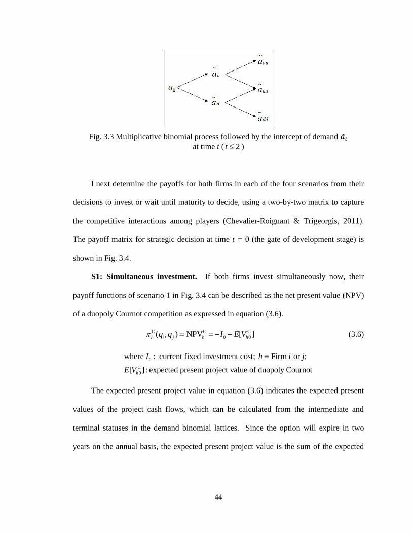
44
Fig. 3.3 Multiplicative binomial process followed by the intercept of demand at time t ( 2t )
I next determine the payoffs for both firms in each of the four scenarios from their
decisions to invest or wait until maturity to decide, using a two-by-two matrix to capture
the competitive interactions among players (Chevalier-Roignant & Trigeorgis, 2011).
The payoff matrix for strategic decision at time t = 0 (the gate of development stage) is
shown in Fig. 3.4.
S1: Simultaneous investment. If both firms invest simultaneously now, their
payoff functions of scenario 1 in Fig. 3.4 can be described as the net present value (NPV)
of a duopoly Cournot competition as expressed in equation (3.6).
C C C
0 0( , ) NPV [ ]h i j h hq q I E V (3.6)
0
C
0
where : current fixed investment cost; Firm or ;
[ ] : expected present project value of duopoly Cournoth
I h i j
E V
The expected present project value in equation (3.6) indicates the expected present
values of the project cash flows, which can be calculated from the intermediate and
terminal statuses in the demand binomial lattices. Since the option will expire in two
years on the annual basis, the expected present project value is the sum of the expected

45
present cash flows from the intermediate statuses of time 1 [E C
1]h and the expected
project value at the expiration (time 2) [ C
2 ]h as shown in equation (3.7).
C 1
0[ ] (1 ) [hE V r E C 2
1 0] (1 ) (1 ) [h r G E C
2 ]h
(3.7)
[E C
1 1]h P C
1(1 )hu P C ;hd
[E C
2 1 2]h PP C
1 2 2 1[ (1 ) (1 )]huu P P P P C
1 2(1 )(1 )hud P P C ;hdd
: probability of an upward at time ( 1,2)tP t t
Firm j
Invest Wait
Fir
m i
Inves
t
(S1) Simultaneous
investment C
C
( , )
( , )
i i j
j i j
q q
q q
(S2) Sequential
investment L
F
( , )
( , )
i i j
j i j
q q
q q
Wait
(S3) Sequential
investment F
L
( , )
( , )
i i j
j i j
q q
q q
(S4) No investment
(Both wait) W
W
( , )
( , )
i i j
j i j
q q
q q
Fig. 3.4 Payoff matrix for strategic decision at time t = 0
(C: Cournot competition, L: leader, F: follower, W: wait)
The right two terms of equation (3.7) can be further defined by finding the
differences between the market-clearing price and the firm’s unit variable cost and then
multiplying the number of the annual planned capacity, as expressed in equation (3.8). In
equation (3.8), C
1h is the stochastic value of the cash flow at time 1 for Firm h. On the
other hand, C
2h includes the stochastic cash flows at time 2 and for the remaining project
life with the total annual growth rate G0 at maturity.

46
C
1 (h 1 )h hc q
C
2 (h 2 0) (1 )h hc q G
(3.8)
where : unit variable cost of Firm ( Firm or ) ;hc h h i j
: annual capacity of Firm ;hq h
1, 2: stochastic market clearing price at time 1, 2
Hence, both the expected value of cash flow at time 1 and the expected project
value at time 2 for Firm h can be computed from their values at each status in Fig. 3.3
with their corresponding probabilities from equation (3.2), given by equation (3.9).
[E C
1 1] [ (h hq P 1) (1 )(u hc P )]d hc
[E C
2 0 1 2] (1 ){ (h hq G PP 1 2 2 1) [ (1 ) (1 )](uu hc P P P P 1 2) (1 )(1 )(ud hc P P )}dd hc
(3.9)
By combining equations (3.6) to (3.9) with the linear (inverse) demand function, the
payoff functions of scenario 3.1 in Fig. 3.4 can be rewritten as in equation (3.10).
C 1
0( , ) (1 ) [h i jq q I r E C 2
1 0] (1 ) (1 ) [h r G E C
2 ]h
1
0 1(1 ) [ (hI r q P u ) (d ' )]d h h hbq bq c
2
0 1 2(1 ) (1 ){hr q G PP 1 2 2 1[ (1 ) (1 )]uu P P P P 1 2(1 )(1 )ud P P ' }dd h h hbq bq c
(3.10)
'where : capacity of Firm 's competitorhq h
S2: Sequential investment (Firm i invests and Firm j waits). In the second
scenario of Fig. 3.4, Firm i invests now and Firm j waits: this scenario makes Firm i the
leader when Firm j invests at time 1 or 2, or makes Firm i a monopolist if Firm j
eventually abandons the project at time 2. Hence, each of the three possible cases will be

47
discussed individually below. Accordingly, the payoff functions of scenario 2 will select
the maximization of these three possible cases.
Case 1: When Firm i invests now, Firm j invests at time 2. In this case, the
payoff function of Firm i will comprise the expected monopolistic profits for the
first two periods [E ( M
1i M
2i ) and the expected duopolistic profits for the
remaining project service life ( C
2i ) as expressed in equation (3.11).
L
0( , ) [i i jq q I E M 1
1 ](1 ) [i r E M 2
2 ](1 ) [i r E C 2
2 0](1 )i r G (3.11)
where L: leader;M: monopoly; [E M
1 1]i P M
1(1 )iu P M ;id
[E M
2 1 2]i PP M
1 2 2 1[ (1 ) (1 )]iuu P P P P M
1 2(1 )(1 )iud P P M ;idd
[E C
2 1 2]i PP C
1 2 2 1[ (1 ) (1 )]iuu P P P P C
1 2(1 )(1 )iud P P C
idd
On the other hand, the current payoff function of Firm j describes the fixed
investment cost of time 2 and the current values of gains from the duopolistic profits after
time 2 (depending on the product diffusion rate in demand) as shown in equation (3.12).
The term C
2j in equation (3.12) is the expected profit of Firm j at time 2 with the
corresponding probabilities.
F 2 2
(2) 2 0( , ) (1 ) (1 ) [j i jq q I r r G E C
2 ]j
(3.12)
where [E C
2 1 2]j PP C
1 2 2 1[ (1 ) (1 )]juu P P P P C
1 2(1 )(1 )jud P P C ;jdd
F
(2) : current profit function of Firm when it is a follower at time 2;j j
2
2 2 0: the fixed investment cost at time 2, (1 )I I I
Case 2: When Firm i invests now, Firm j abandons at time 2. In this case, Firm
i will simply gain the monopolistic profits during its product service life and Firm
j’s payoff value is 0 as shown in equation (3.13). Term M
2i in equation (3.13)

48
is the expected monopolistic project value of Firm i at time 2 with the
corresponding probabilities.
M 1
0( , ) (1 ) [i i jq q I r E M 2
1 0] (1 ) (1 ) [i r G E M
2 ]i
( , ) 0j i jq q
(3.13)
[E M
2 1 2]i PP M
1 2 2 1[ (1 ) (1 )]iuu P P P P M
1 2(1 )(1 )iud P P M
idd
Case 3: When Firm i invests now, Firm j invests at time 1. In this case, the
payoff function of Firm i will comprise the expected monopolistic profit in the
first period and the expected duopolistic profits for the remaining project service
life as shown in equation (3.14).
L
0( , ) [i i jq q I E M 1
1 ](1 ) [i r E C 2
2 0](1 ) (1 )i r G (3.14)
On the other hand, the current payoff function of Firm j describes the fixed
investment cost of time 1 and the gains from the expected duopolistic profits after time 1
(depending on the product diffusion rate in demand), as shown in equation (3.15).
F 1
(1) 1( , ) (1 ) [j i jq q I r E C 2
2 0](1 ) (1 )j r G (3.15)
1 1 0
F
(1)
where : the fixed investment cost of time 1, (1 ) ;
: current profit function of Firm when it is a follower at time 1j
I I I
j
Of all the above three cases in scenario 2, Firm i has a fixed setting to invest at time
0, but Firm j instead has three possible moves. Since Firm i has only one move, the
payoff functions of scenario 2 will thus mainly depend on Firm j’s decision. The
maximization of these three possible moves from Firm j’s decision can be expressed by
equation (3.16), which combines equations (3.12), (3.13) and (3.15).

49
L F*
F* F F
(1) (2)
Firm : ( ( , ))
Firm : ( , ) max[ ( , ), ( , ),0]
i j i j
j i j j i j j i j
i q q
j q q q q q q
(3.16)
S3: Sequential investment (Firm j invests and Firm i waits). In the third
scenario of Fig. 3.4, Firm j invests now and Firm i waits. This scenario allows Firm j to
be a leader if Firm i invests at time 1 or 2, or to be a monopolist if Firm i eventually
abandons the project at time 2. Scenario 3 is the same concept as scenario 2 but with the
firms having opposite roles. Hence, Firm j has only one move, so the payoff functions of
scenarios 3 will mainly depend on Firm i’s decision. Similarly, the payoff functions of
scenario 3 can be written to maximize the three possible moves from Firm i’s decision as
expressed in equation (3.17).
F* F F
(1) (2)
L F*
Firm : ( , ) max[ ( , ), ( , ),0]
Firm : ( ( , ))
i i j i i j i i j
j i i j
i q q q q q q
j q q
(3.17)
S4: No investment (both wait). If both firms wait now, their payoff functions can
be viewed as the present value of a shared American call option with three possible
investment actions within two periods: invest at time 1, invest at time 2, or abandon at
time 2. With the evolution of the demand binomial tree, I can value each strategy
between the firm and its rival by working the tree backward (Chevalier-Roignant &
Trigeorgis, 2011). At maturity, there is a two-by-two payoff matrix in each of the
terminal statuses as shown in Fig. 3.5. When firms decide to invest or abandon the
project at time 2, there are three combined strategies: simultaneous investment, monopoly
investment, and no investment. Simultaneous investment means that if both invest at
time 2, a Cournot duopoly game is formed and their stochastic payoff functions can be
expressed as shown in equation (3.18). Monopoly investment means that only one of

50
them invests at time 2, so that the investing firm gains the stochastic monopolistic
investment and its rival’s value is zero as shown in equation (3.19). No investment gives
both firms zero value since they abandon the project simultaneously at time 2.
Firm j
Invest Abandon
Fir
m i
Inves
t (1) Simultaneous
investment
2 ( , )i i jq q
2 ( , )j i jq q
(2) Monopoly
investment
2 ( , )i i jq q
Ab
an
don
(3) Monopoly
investment
2 ( , )j i jq q
(4) No investment
(Abandon)
Fig. 3.5 Payoff matrix for strategic investment decision at time t = 2
2 2( , )h i jq q I C
2 2h G (3.18)
C 2
2 (h hbq 2 ' ) h h hbq c q
2 2( , )h i jq q I M
2 2h G (3.19)
M 2
2 (h hbq 2 )h hc q
Thus, the resulting equilibrium outcomes in the end statuses can be obtained from
the payoff matrices of time 2 by applying the Nash equilibrium with the best response
analysis, where the competitive outcomes at time 2 in each status are noted as
* *
2 ( , ),i i jq q * *
2 ( , )j i jq q

51
Next, working in the previous period (time 1) of the binomial tree, there is a payoff
matrix in each of the intermediate statuses as shown in Fig. 3.6. When the firms decide
to invest or wait at time 1, there are three combined strategies: simultaneous investment,
sequential investment, and no investment. Simultaneous investment means that if both
invest at time 1, a Cournot duopoly game is formed and their stochastic payoff functions
can be expressed in equation (3.20).
1
1 1 1( , ) (1 ) (1 ) [h i jq q I r G E C
2 ]h (3.20)
[E C
2 2] (h P C
2 2) (1 )(h P C
2');h
C 2
2 (h hbq 2 ' ) ;h h hbq c q
'2: the up move at time 2;2 : the down move at time 2
Firm j
Invest Wait
Fir
m i
Inves
t
(1) Simultaneous
investment
1( , )i i jq q
1( , )j i jq q
(2) Sequential
investment
1( , )i i jq q
1( , )j i jq q
Wait
(3) Sequential
investment
1( , )i i jq q
1( , )j i jq q
(4) No investment
(Both wait)
1( , )i i jq q
1( , )j i jq q
Fig. 3.6 Payoff matrix for strategic investment decision at time t = 1
Sequential investment means that if one of the firms invests at time 1, the other
waits, comprising two possible cases: actual sequential investment and monopoly
investment, as shown in Fig. 3.6. If it is an actual sequential investment, one invests at

52
time 1 and the other invests at time 2. If it is a monopoly investment, one of them invests
at time 1 and gains the monopoly. Its rival abandons the project at time 2 with zero
value. The payoff functions will be the maximum for sequential investment. Equation
(3.21) describes the payoff functions of sequential investment by maximizing the above
two cases for scenarios 2 and 3 in Fig. 3.6, respectively. No investment means that if
both firms wait at time 1, their payoff functions can be computed as the option value
from the optimal matrix outcome of time 2 with the risk neutral probability qr, as
expressed in equation (3.22).
Scenario 2: ( 1,i 1) max[(j L
1,i F
(2) ), (j M
1 ,0)]i
Scenario 3: ( 1,i 1) max[(j F
(2) ,i L
1), (0,j M
1)]j
(3.21)
L
1,i L
1: payoff when Firm , is a leader at time 1;j i j
F
(2) ,i F
(2): payoff when Firm , is a follower at time 2j i j
[ 1( , ),i i jq q 1( , )]j i jq q [rq
*
2 (1 )i rq *
2'i
1 fr,
rq *
2 (1 )j rq *
2'j
1 fr] (3.22)
*
2h * *
2( , ) : equilibrium results at time 2 for Firm or h i jq q i j
Therefore, the resulting equilibrium outcome in each intermediate status can be
obtained from the payoff matrices of time 1 by applying the Nash equilibrium with the
best response analysis, where the competitive outcomes are noted as
* *
1( , ),i i jq q * *
1( , )j i jq q Finally, the payoff functions of scenario 4 at time t = 0 in Fig.
3.4 are the competitive outcomes at intermediate statuses obtained from the payoff
matrices of time 1 by applying the Nash equilibrium with the best response analysis, as
shown in equation (3.23).

53
W W[ ( , ), ( , )]i i j j i jq q q q [rq
* (1 )iu rq *
id
1 fr,
rq * (1 )ju rq
*
jd
1 fr] (3.23)
*
1h * *
1( , ) : equilibrium results at time 1 of Firm (timeh i jq q h or )u d
3.2.3 Strategic decisions and the planned capacity
The profit functions of both firms in each of the four scenarios at time t = 0 are
derived and defined in section 3.2.2 above. One firm’s output choice (qh) is not the only
factor that influences the product market price; the rival’s choice (qh’) also influences it.
In order to find the equilibrium results of the payoff matrix at time t = 0, the Nash
equilibrium outputs (qi, qj) are applied, where each firm’s capacity choice is the best
response to the other’s optimal capacity decision (Chevalier-Roignant & Trigeorgis,
2011). Therefore, one firm’s optimal capacity can be determined by taking the first-order
condition for the firm’s profit maximization and the rival’s capacity choice as given. The
details of Nash equilibrium outputs for the four scenarios are derived separately in
Appendix A and summarized in the payoff matrix shown in Fig. 3.7. Finally, the
resulting equilibrium for the gate decision of the development stage can be obtained from
the payoff matrix at time t = 0 (Fig. 3.7) by applying the Nash equilibrium with the best
response analysis, where the competitive outcomes are noted as * * * *[ ( , ), ( , )]i i j j i jX q q X q q
with the optimal capacity * *( , )i jq q .

54
Firm j
Invest Wait
Fir
m i
Inves
t
(S1) Simultaneous
investment C * *
C * *
( , )
( , )
i i j
j i j
q q
q q
(S2) Sequential
investment L F **
F **
( ( , ))
( , )
i j i j
j i j
q q
q q
Wait
(S3) Sequential
investment F **
L F **
( , )
( ( , ))
i i j
j i i j
q q
q q
(S4) No investment
(Both wait) W * *
W * *
( , )
( , )
i i j
j i j
q q
q q
Fig. 3.7 Profit maximization for each strategic investment decision at time t = 0
3.2.4 Benchmark: the NPV approach
Suppose the two firms are competing in the target marketplace and Firm i’s and j’s
unit variable costs ci and cj are constant ( , 0,i j i jc c c c ). In the settings of the
benchmark, the demand will have the constant expected growth rate g. In addition, the
profit of Firm i is based on its market share of the overall product quantity in the target
market. To earn the maximum overall profit, the industry chooses to produce the output
that equals their average marginal cost to marginal revenue (Chevalier-Roignant &
Trigeorgis, 2011). Therefore, the equilibrium quantity produced in the industry is shown
in equation (3.24) and Appendix A.
0
2
a cQ
b
(3.24)
where : average marginal cost ( ) / 2i jc c c
The capacity of Firm i is computed by its estimated market share ω of the total
supply quantities in the industry and represents the degree of dominance that Firm i has
within the particular market. To simplify the definition, the market share is estimated by

55
the unit variable costs from both firms (ci, cj). As I assume that there is only one
competitor, the rival’s unit variable cost directly influences Firm i’s market share as
expressed in equation (3.25). Finally, the resulting equilibrium profit of Firm i by the
NPV approach can be expressed in equation (3.26) and is provided in Appendix A.
j
i j
c
c c
(3.25)
0 0
0 0
( )( 2 )NPV
4i
i
G a c a c cI
b
(3.26)
1
1where ( )
1
mN
m
gG
r
3.3 Case Study
In this section, a numerical example is demonstrated with the analysis and
comparison of a project with single output. The market demand follows a binomial
lattice with the product life cycle as defined in section 3.2.1. The illustrations of a
binomial lattice integrated with product diffusion and the relevant market structure
patterns are presented in section 3.3.1. Accordingly, the scenarios of payoff matrices in
the option-game framework are calculated and shown in Section 3.3.2. I further compare
my approach to a benchmark and observe the results of the strategic decision and the
quantity of the planned capacity. I chose NPV as the benchmark because it is the most
common and widely used conventional financial method in gate-criteria. In addition,
further sensitivity analyses of the project payoffs and the option values are studied based
on the assumptions of the parameters in section 3.3.3.

56
Suppose Firm i is assessing an individual project at gate-decision of the
development stage in the NPD process, where all the individual projects have been
screened and investigated through the strategic buckets approach in the early stages (as
described in section 3.2). Some portions of the buckets are the projects with the specific
dimensions of high risk, uncertain market, short life cycle, a potential competitor, and a
rapidly changing environment. Firm i will need to evaluate these categories of projects in
the gate decision before proceeding to the product development stage. The questions for
Firm i are how to evaluate this project at this gate-decision, whether this project should
proceed to the next stage, and if so, what the optimal quantity of planned capacity will be.
Firm i and its rival (Firm j) are in a duopoly and share a delay option to invest in an
NPD project where the option will expire in two years (T = 2). Both firms make their
decisions on an annual basis (Δt = 1), and the project will operate for a finite service life
of N = 4 years with the same interest rate r = 12% and risk free rate rf = 5%. The current
demand is given as Q0 = 750, with an expected yearly growth rate of g = 8% and an
expected standard deviation of σ = 50%. Both firms have the same current fixed
investment cost (I0 = $34,500), which would be reduced 15% each year (i.e., I1 =
$29,325; I2 = $24,926.25). Firm i has a cost advantage where Firm i’s unit variable cost
(ci = $10) is less than Firm j’s (cj = $15). The current (inverse) demand function is given
as 0 50 0.05p Q . Suppose that the firms’ roles and sequences are not determined a
priori because of the business strategy in the categorized buckets of projects. Moreover,
due to the considerations of the product life cycle, reduced fixed investment cost over
time, and asymmetric unit variable costs, the firms are also not sufficiently distinct.

57
Hence, mixed strategies may give further insights and help determine the values of
potential decisions.
3.3.1 Demand structure patterns with product diffusion
With the above given information (g = 8%, σ = 50%, rf = 5%, T = 2, Δt = 1), I can
calculate the parameters of the binomial lattice into equation (3.1) and obtain the
following: u = 1.6487, d = 0.6065, qr = 0.4255, 1-qr = 0.5745, P = 0.58, and 1-P = 0.42.
The concept of product life cycle is integrated into the binomial lattice depending on
when the new product is introduced to the market. There are three integrated demand
structures considered when the project diffusion is incorporated with the binomial lattice:
(1) if either firm invests now, (2) if the project is first invested at time 1, and (3) if the
project is first invested at time 2.
In the first demand structure, the upward probabilities in the first period and second
period can be computed from equation (3.2) as 0.71 and 0.54, respectively. The
remaining two-year product life after maturity will have the growth rates of -0.13 and -
0.21 for years 3 and 4, respectively, from equation (3.3). Fig. 3.8 shows the demand
binomial lattice with product diffusion of N = 4 years product life cycle and the
cumulative probabilities of demand at time 2 in the first demand structure, where the
cumulative demand indicates demand at and after time 2 at each end status for the
observation of the total future demand distribution.
To compare the demand distribution of a binomial lattice with product diffusion to
that of a standard one, I assume the standard binomial lattice follows a constant growth
rate (g = 8%) in a finite project life. Fig. 3.9 shows that the demand values at each end
status of the standard method are slightly overestimated without considering product

58
diffusion. In addition, when product diffusion is considered, if the product is introduced
to market next period, the probability of the upward status at maturity is increased.
Moreover, the expected demand at time 2 is computed as 3,141.06 units, which is about
10.65 percent lower than that of the standard method. The main reason for the difference
is that the standard binomial lattice is assumed to have a constant annual growth rate. In
contrast, when using the product diffusion concept, the annual growth rate will be re-
calculated based on the different market structure patterns.
Fig. 3.8 The binomial lattice with product diffusion of N = 4 product life cycle
(The first demand structure pattern: if either firm invests now)
The binomial lattices with product diffusion and the demand probability
distributions at time 2 for the second and third demand structure patterns are shown in

59
Appendix B1. Overall, the demand distribution will be affected by when the new product
is introduced to the market (for all three demand structures). In other words, if either of
the firms invests in the project in the early periods, the demand distribution at maturity
will not be optimistic. Furthermore, in all three demand structures, the expected demands
at maturity of my approach are 10.65%, 3.06%, and 8.35% lower than those of standard
ones (in the order of the demand structure), due to the consideration of product diffusion.
In summary, the demand distribution at T = 2 and the annual growth rate after maturity
can be overestimated without integrating the concept of product diffusion into a demand
binomial lattice.
Fig. 3.9 Demand distribution at T = 2
(The first demand structure pattern: if either firm invests now)
3.3.2 Strategic decisions and the optimal planned capacity
Appendix B2 shows the calculations in each scenario and the payoff matrices in the
intermediate and terminal statuses. The results are summarized in Table 3.1. Applying
the Nash equilibrium concept, the payoff matrix at time t = 0 can be obtained from
combining the four scenarios of Appendix B2. In Table 3.1, both firms will gain negative
payoffs if they invest simultaneously. The optimal strategic decision will be for both
0.3834
0.4832
0.1334
0.3364
0.4872
0.1764
0
0.1
0.2
0.3
0.4
0.5
0.6
0 1000 2000 3000 4000 5000 6000 7000
Pro
bab
ilit
y
Demand at and after maturity (units)
Demand distribution at T=2 (1st demand pattern)
Product
diffusion
Standard
binomial

60
firms to wait. The second best outcome will be for either firm to take the action opposite
of the rival’s to gain the monopoly profit. Hence, based on these competitive outcomes,
the firms should not both invest at the same time now, but carefully observe the rival’s
move. The optimal planned capacities in each scenario are shown in Table 3.2.
Table 3.1 Payoff matrix at time t = 0
πi, πj Firm j
Invest Wait
Firm i Invest -$4,583.59 -$16,028.75 $17,220.72 $0.00
Wait $0.00 $9,136.94 $17,178.73 $9,147.47
Table 3.2 The optimal planned capacity
qi, qj Firm j
Invest Wait
Firm i Invest 467 367 614 0
Wait 0 564 873 773
In order to compare the results to a benchmark, I use the NPV approach, the
common and widely used conventional financial method in gate-criteria. Appendix B3
shows the details of the calculation of NPV. The result of NPV is -$17,022.6 with an
average annual planned capacity of 225 units. Hence, by this gate-criterion, the negative
value of NPV makes the current project a kill/no go decision. Based on the NPV
criterion, the project should be abandoned, but the option-game approach assesses the
value of a project’s flexibility and suggests putting the project on a waiting list (Fig. 3.1)
to see if any new information appears.

61
3.3.3 Sensitivity analyses
As a numerical example has been demonstrated, in this section, further sensitivity
analyses of the project payoffs and the option values are studied based on the
assumptions of the parameters (the expected growth rate g, the expected standard
deviation σ, the unit variable costs ci, cj, and the project service life N). All other
parameters are the defaults from section 3.3.2. The results of the sensitivity analyses in
each of the four parameters are shown in Appendix B4. Overall, the results show that the
payoffs and option values of Firm i in each scenario become larger when increasing the
value of the parameter. In scenario 2 (Firm i invests and Firm j waits at time t = 0), with
the growing standard deviation, or project service life, Firm i may gain a lower payoff
from the next period of competitive outcome at time 1, since Firm j may change its
investment decisions due to the increasing option value. Therefore, even though Firm i
has the cost advantage (i.e., unit variable cost), their project profits and/or option values
could be influenced and partitioned by Firm j’s investment decision when the project
variability or product service life is high.
3.3.4 Interpretation of the results
This case study shows that the integration of product diffusion into a binomial
lattice of demand influences the demand distribution at T = 2, the probability of an
upward in demand, and the annual growth rate when compared to a standard one (with a
constant growth rate in a finite project life). The results and implications are consistent
with Bollen’s study (1999). For the gate-criterion, this approach suggests that the firms
should not invest simultaneously now, but carefully observe the rival’s move as long as
there is still value in the decision to wait. While the conventional NPV criterion gives a

62
kill/no go decision for this project, this approach allows for a “wait-and-see” action.
Therefore, instead of abandoning a project based on a kill/no go decision, this approach
determines that the project is worth re-investigating in the next round of periods. On the
other hand, the optimal planned capacities in each of the four scenarios can be obtained
by the Nash equilibrium, which can provide a more strategic preliminary planned
capacity for the scale of the new product development than that of the NPV approach
with an average annual planned capacity. The sensitivity analyses show that in scenario
2, option values and project payoffs of Firm i can be partitioned by its rival when either
the parameter of project variability or product service life is high. As a numerical
example cannot generalize the results, the next section provides further validation and
discussion.
3.4 Validation and Discussion
The option value approach incorporates potential flexibility, which the NPV
approach does not consider. In this section, I use my approach to verify the value of
managerial flexibility in a project. I also discuss the research limitations and possibilities
for future research.
3.4.1 Validation
The academic literature has confirmed the value of flexibility, which the NPV
approach lacks. Hence, I mainly focus on the value of flexibility provided by the option-
game technique. It has been proved that the optimal exercise policy for the owner of an
American call option is to hold the option until maturity (Hull, 2008). Accordingly, since
the delay option in this model can be viewed as an American investment option, I will
validate this model as a European option at maturity for the sake of simplicity.

63
Moreover, Chevalier-Roignant and Trigeorgis (2011) have illustrated the investment
decisions of a European option at maturity in an asymmetric Cournot duopoly. They
conclude that both firms invest simultaneously as an asymmetric Cournot when demand
is high; a low-cost firm invests as monopoly but a high-cost firm does not when demand
is in the intermediate; no one invests when demand is low. From their findings, I can
employ these sets of investment decisions in each status of maturity as a priori for the
two-year binomial tree as shown in Fig. 3.10.
Fig. 3.10 Investment decisions and payoffs at maturity in an asymmetric Cournot
duopoly (Chevalier-Roignant & Trigeorgis, 2011)
Consequently, with these payoff functions in each status at maturity (Fig. 3.10), I
can compute their option value, which is also called strategic net present value (SNPV),
at time t = 0. When NPV is subtracted from the value of SNPV, the option premium is
obtained. In this way, I can demonstrate the value of managerial flexibility via the
option-game approach. More specifically, option premium is used as an indicator in the

64
option-game approach to measure the exclusive strategic value of flexibility, which the
NPV method lacks.
Before calculating the option value, Firm i’s resulting equilibrium profit needs to be
determined. The details of calculation of resulting equilibrium profits are provided in
Appendix C. The project service life is assumed to be N = 4 years. Hence, the
equilibrium profits of asymmetric Cournot and monopoly for Firm i are shown in
equations (3.27) and (3.28), respectively. With equations (3.27) and (3.28) and the risk-
neutral probability, the present value (t = 0) of the strategic investment option for Firm i
can be computed as expressed in equation (3.29). Finally, option premium (OP) is
obtained with equation (3.29), subtracting the value of NPV, as expressed in equation
(3.30).
2( , )iuu i jq q I
( 2
22 )uu i jc c G
9b (3.27)
2( , )iud i jq q I
( 2
2)ud ic G
4b (3.28)
00SNPVi
2 2iuu rq (1 )iud r rq q
2(1 )fr
(3.29)
00 00 00OP SNPV NPVi i i
2 2iuu rq (1 )iud r rq q
2(1 )fr
0 0
0
( )( 2 )
4
iG a c a c c
Ib
(3.30)
As the value of option premium can be influenced by multiple parameters, further
sensitivity analyses can provide the trends with specific parameters (the expected
standard deviation of demand σ, the expected yearly growth rate g, the ratio of firms’ unit

65
costs βvc, and the annual reduced rate of the fixed investment cost λ). All other
parameters are set as the defaults from the previous section. The results show that the
expected standard deviation of demand (σ) is the most critical parameter in the option
premium. As shown in Fig. 3.11, option premium grows dramatically with the increasing
value of σ.
Fig. 3.11 Sensitivity analysis of option premium by changing
the expected standard deviation of demand σ
On the other hand, increasing either the expected yearly growth rate (g) or the ratio
of the firms’ unit costs (βvc) increases option premium only slightly, as shown in Figs.
3.12 and 3.13, respectively. It is noted that when Firm j’s unit variable cost is much
greater than Firm i’s, the ratio of βvc is larger. Hence, Firm i can take more cost
advantage.
0
10000
20000
30000
40000
50000
60000
70000
80000
90000
100000
0.1 0.2 0.3 0.4 0.5 0.6 0.7 0.8 0.9
Op
tio
n p
rem
ium
($
)
Change of σ

66
Fig. 3.12 Sensitivity analysis of option premium by changing the expected yearly
growth rate g
Fig. 3.13 Sensitivity analysis of option premium by changing the ratio of firms’
unit costs βvc
The last parameter, λ, is defined as the annual reduced rate of the fixed investment
cost. It has an upward trend on option premium when the fixed investment cost drops
0
10000
20000
30000
40000
50000
60000
70000
80000
90000
100000
0.05 0.06 0.07 0.08 0.09 0.1 0.11 0.12 0.13
Op
tio
n p
rem
ium
($
)
Change of g
0
10000
20000
30000
40000
50000
60000
70000
80000
90000
100000
1.1 1.2 1.3 1.4 1.5 1.6 1.7 1.8 1.9
Op
tio
n p
rem
ium
($
)
Change of βvc

67
greatly over time. Therefore, a rising reduced rate of λ will also positively impact option
premium as shown in Fig. 3.14.
Fig. 3.14 Sensitivity analysis of option premium by changing
the annual reduced rate of the fixed investment cost λ
In summary, option premium is used as an indicator in the option-game approach to
measure the exclusive strategic value of flexibility, which the NPV method lacks. The
results of sensitivity analyses imply that option premium is positively influenced by the
dimensions and characteristics in the buckets of projects in the area of interest.
Particularly, the high risk and uncertain projects in the market have higher value of
flexibility in this approach, while the NPV method does not consider the uncertainty.
Moreover, the above results of the demonstrated option premium are based on the
assumption of a European option. An American option is generally more valuable than a
European option, since it can be exercised at any time before maturity. Therefore, the
0
10000
20000
30000
40000
50000
60000
70000
80000
90000
100000
0.1 0.15 0.2 0.25 0.3 0.35 0.4 0.45 0.5
Op
tio
n p
rem
ium
($
)
Change of λ

68
American investment option in this approach can provide an equivalent or even better
option premium.
3.4.2 Limitations and possible extensions
As I focus on individual project assessment at gate-criterion of the development
stage in the NPD process (Fig. 3.2), this gate criterion will determine whether the project
goes to the active development level in the next stage of development. When the market
condition of the project is highly uncertain, the option-game approach can assess the
value of flexibility, which is inadequately assessed in the NPV method. While the NPV
criterion offers a go/kill decision, the option-game approach instead provides a go/wait
decision. The decision to wait is especially significant for risky projects. Both passive
and active strategies can be used in a delay option (Mun, 2006). In the passive wait-and-
see strategy, the project will go to the waiting list. Meanwhile, the firms wait and gather
new information, and the project will be re-investigated in the next round of periods.
Alternatively, they may also use an active market research strategy. Instead of waiting
until the next period, firms may budget more for marketing in order to collect
information. The maximum value to spend on marketing information is the value of
option premium.
The gate-criteria for projects are multidimensional in the NPD process. Especially
in the early and middle stages, the financial data are inadequate and inaccurate. Multiple
qualitative and quantitative factors are not considered thoroughly in this option-game
framework, such as gathering new information, technical success rate, product quality,
periodic linking to business strategy, etc. Hence, most companies use other supportive
methods in conjunction with financial models in their management (Cooper et al., 2001),

69
such as scoring models and QFD (quality function deployment). Most importantly,
unlike the conventional financial methods, the option-game approach provides a project
evaluation of managerial flexibility. Combined with other standard approaches, the gate-
criteria for project assessment can become more comprehensive.
3.5 Summary and Conclusion
In this chapter, I develop an option-game framework for the gate-criterion of a
project in the NPD process for which the market demand is uncertain and the new
product is in a short life cycle. The decision to delay adds flexibility, allowing firms to
use a passive wait-and-see strategy or an active market research strategy while delaying.
The standard conventional financial method in gate-criteria, NPV, is inadequate when
projects face uncertainty. Hence, while the NPV criterion offers a go/kill decision, the
option-game approach instead provides a go/wait decision.
The results of sensitivity analyses of option premium imply that option premium is
positively influenced by the dimensions and characteristics of the project buckets on
which I focused. Predominantly, high risk and uncertain projects have a higher value of
flexibility.
To consider a short product life cycle, I integrate product adoption rates (Rogers,
1995; Bollen, 1999) into the option-game framework for evaluating an NPD project. I
further develop the formal mathematical option-game framework in the discrete-time
analysis when dealing with an American investment option in a finite project life. In this
model, I consider the results of both simultaneous and sequential investment decisions in
each scenario of the duopolistic game. Moreover, I can also use this technique to
compute the optimal selection of the planned production capacity. The optimal planned

70
capacities in each of the four scenarios can be obtained by the Nash equilibrium, which
can provide a more strategic preliminary planned capacity for the scale of the new
product development.
The strategic buckets approach in the early stages of the NPD process links the
business strategy and the portfolios (Cooper et al., 1997). The option-game framework in
the gate-criterion of the development stage allows further inspection and examination of
the individual projects in the development process. Most importantly, in contrast to the
commonly used financial methods, the option-game approach provides a project
evaluation of managerial flexibility. Many companies use other supportive methods in
conjunction with financial models in their management (Cooper et al., 2001), such as
scoring models and QFD. Combined with other standard approaches, the gate-criteria for
project assessment become more comprehensive.

71
Chapter 4 Assessing Managerial Flexibility in a New Product
Development Project: An Option-Game Approach
in a Duopoly with Bayesian Analysis
Abstract
Effective gates are central to the success of an idea-to-launch product development
process. The most common financial gate-criterion, the net present value (NPV) method,
is insufficient when the success of a project is uncertain. Alternatively, the real-option
valuation is inadequate when a strategic decision is affected by the moves of the
competition. In this chapter, I develop the idea for a discrete option-game valuation
framework that explicitly incorporates statistical decision theory in the form of Bayesian
analysis. The high volatility in an initially uncertain market is diminished via consumer
information updates and by understanding the requirements and preferences of the
customers. In addition, an inverse measure of product differentiation is included in the
option-game mechanism to describe whether two goods are homogeneous, substituted, or
independent, and to what degree. I introduce this approach as a gate-criterion to evaluate
a new project at the gates of the development stages in a new product development
(NPD) process. In a highly uncertain target market, evidence of high demand warrants a
“go” action, especially when a firm has the cost advantage in competing with its rival's
highly comparable product. This research has important implications for stage-gate

72
management when investigating an NPD project in the duopoly game during the product
development process. By this approach, industry players can make the proper strategic
decisions in a project assessment at the gates of the development stages.
Keywords: option-game, asymmetric duopoly, Cournot competition, product
differentiation, gate-criteria, new product development, Bayesian analysis
4.1 Background
Effective gates are central to the success of an idea-to-launch product development
process. Yet the majority of the businesses in Cooper and Edgett’s study (2012)
indicated that they lacked a fact-based and objective approach to decision-making at the
gates of the new product development (NPD) process.
4.1.1 New product development (NPD)
NPD is widely regarded as a vital source of competitive advantage (Bessant &
Francis, 1997). An NPD process from idea to launch consists of multiple stages, such as
the project screening, monitoring, and progression frameworks of Cooper’s stage-gate
approach. A stage-gate process is a conceptual and operational blueprint for managing
the NPD process (Cooper, 2008). Nowadays, instead of a standardized mechanistic
implementation process, there are many different versions to fit different business needs
(Cooper, 2008). In an idea-to-launch product process, each stage has defined procedures
and requires the gathering of relevant information. Following each stage is a “gate”
where go/kill decisions are made to manage the risks of new products and to serve as a
quality-control checkpoint to continue moving the right projects forward (Cooper &
Edgett, 2012; Cooper, 2008; Carbonell-Foulquié et al., 2004).

73
Cooper (2008) explains the stage-gate process as being very similar to that of
buying a series of options on an investment: as each stage costs more than the preceding
one, the initial amount of cost is analogous to the purchase of an option. Then the
decision of whether or not to continue investing in the project is made at the gate
(maturity), while new information is gathered during the stage. Indeed, the flexibility of
the real-option approach corresponds to the structure of the NPD process, allowing
developers to build options into products and projects during decision-making, especially
in areas of uncertainty (Mun, 2006). Huchzermeier and Loch (2001) incorporated the
operational sources of uncertainty with real-option value of managerial flexibility and
introduced an improvement option to take corrective actions during the NPD process for
the purpose of better product performance. However, a major problem with this
approach is the limited knowledge of evaluating projects and the difficulty of making
critical go/kill decisions throughout the entire development process (Schmidt &
Calantone, 1998; Carbonell-Foulquié et al., 2004), especially in a rapidly changing and
competitive environment.
4.1.2 Problem statement
Though both researchers and practitioners agree on the significance of gate-criteria
(Carbonell-Foulquié et al., 2004; Agan, 2010), gates are rated as one of the weakest areas
in product development (Cooper, 2008; Cooper, Edgett, & Kleinschmidt, 2002, 2005).
Only 33 percent of firms have rigorous gates throughout the NPD process (Cooper,
Edgett, & Kleinschmidt, 2002, 2005). In too many companies, gates either do not exist
or are not effective, allowing numerous bad projects to proceed (Cooper, 2008; Jenner,
2007; Cooper & Edgett, 2012). In addition, almost two-thirds of the respondents in

74
Cooper and Edgett's study (2012) indicated that gatekeepers’ contributions were of low
quality. With a lack of robust and transparent decision-making criteria, gatekeepers often
implement stage-gate decisions with the naive belief that using opinion and even personal
agenda is effective (Cooper, 2008).
Moreover, since voice-of-the-customer input is identified as one of the drivers of
success in an NPD process (Cooper & Edgett, 2012; Calantone et al., 1995), the criteria
in a project assessment should involve the understanding of customer needs (Scott, 2000;
Bessant & Francis, 1997; Griffin & Hauser, 1996). Due to shorter product life cycles in
fast-paced industries, it is not necessary to wait for perfect information at the pre-defined
gate for decision-making. Stages can be overlapped in a stage-gate process by using
spiral development, allowing product development to continuously incorporate valuable
customer feedback into product design during an NPD process until the final product is
closer to customers’ ideal (Cooper, 2008). In contrast to traditional uncertainty reduction
methods in real-option theory, which are a passive process (Miller & Park, 2005),
Artmann (2009) derived the Bayesian updating formulation for the market requirement
distribution and integrated this mechanism into a real-option framework. In addition to
the problem of predicting product demand, decision makers must also consider what
competing companies are doing. Because “similar product developments exist in greater
or lesser degrees in almost all product areas” (Smith, 1995), the competitor's involvement
in a dynamic setting could influence one firm’s output choice in the target market.
Hence, in a competitive marketplace, the real-option valuation methods fall short in
resolving the dilemma when the moves of a rival are involved (Ferreira et al., 2009).
Recently, however, Smit and Trigeorgis (2006) introduced the concept of “option-game,”

75
combining real-option (which relies on the evolution of prices and demand) and game
theory (which captures the moves of competitors) to quantify the value of flexibility and
commitment.
4.1.3 The scope of this chapter
Owing to “too many projects in the pipeline” (Cooper, 2008), I am interested in
decision-making at the gates of an NPD process, particularly involving new information
from a competitor’s interactions and from the requirements and preferences of the
customers. Ronkainen (1985) pointed out that the go/kill decision-making at each gate
should vary across product development stages. Moreover, Cooper (2008) indicated that
most contributions to higher success rates are from the front end of stage-gate decision-
making, where serious financial commitments are started during the go-to-development
stages. Therefore, this chapter focuses specifically on the outset of the development
stages and the iterated sub-decisions of prototyping and testing within the development
stages as shown in Fig. 4.1.
In contrast to the assumptions in chapter 3, I assume that a new project is competing
with a latent product to an inverse measure of product differentiation in the market at the
outset of the development stages. During the sub-decision gates of development (Fig.
4.1), two kinds of new information about market risks are considered: a parameter of one
competitor’s (inverse) product differentiation and the requirements and preferences of the
customers. In other words, one competitor may invest in a related project during the
development stages, when information about the degree of (inverse) product
differentiation might be unknown or uncertain at the outset. While I assumed product
homogeneity in chapter 3, I relax this assumption here and assume that the firms are

76
producing differentiated goods. Two products from two firms are differentiated when
there are actual substitute products but not perfect substitutes (Motta, 2004). In addition,
realizing the increasing importance of customer orientation (Sun, 2006), companies target
a new project at a certain domain of market segmentation, according to the requirements
and preferences of the customers. Yet prediction of customers’ requirements is difficult
because customers do not necessarily realize what their future needs are in the early
stages of product development (Artmann, 2009), making it difficult for producers to
estimate the nature of market demand (Smith, 1995).
Fig. 4.1 Decision-making during the stages of product development
As time progresses during the stages of development (Fig. 4.1), variations in
demand can be diminished by effective use of updated information about the
requirements and preferences of customers. In addition, managerial flexibility should be
considered when a latent product with a certain degree of (inverse) product differentiation
is present in the future competing market. Consequently, considering the above two

77
factors, I propose a discrete option-game valuation framework that explicitly incorporates
statistical decision theory in the form of Bayesian analysis in an NPD project. In view of
the fact that projects are rarely killed at gates after the stage of idea screening (Jenner,
2007), I introduce this approach as a rigorous gate-criterion to evaluate a new project
during the stages of development (Fig. 4.1). As Anderson (2008) pointed out, successful
management of current product development requires the overall integration of strategy,
process, measurement of performance, and continuous improvement. Therefore, this
product development process is discussed in the context of strategic portfolio
management. Hence, this method is based on the strategic buckets method for NPD
projects and is tailored for products in the dimensions of high variability in the initial
markets and uncertainties about latent and competitive products.
As this research builds on concepts that have been previously proposed but not fully
developed, the relevant literature concepts have been reviewed and discussed above. The
remaining parts of this chapter are organized as follows. In section 4.2, I define the
model description and develop this work by using an extended version of the former
structure for my valuation model. The theory of Bayesian analysis is integrated with a
valuation model that allows updating the variability of a target market. In addition, a
latent rival’s product development in a certain degree of (inverse) product differentiation
is considered in the option-game approach. In section 4.3, I provide a case study to
demonstrate the model and compare the results with two benchmarks. The first
benchmark is the NPV method, used to represent the actions of go/kill at the outset of
development stages and the action of go for the remaining NPD process to highlight the
many industrial problems. The second benchmark is based on Artmann’s study (2009),

78
in which a real-option framework is incorporated with Bayesian analysis. In section 4.4,
I further validate my valuation model against the benchmarks and discuss the results.
Section 4.5 summarizes the results and concludes the chapter.
4.2 Model Development
Suppose that projects are initially screened and selected through the strategic
buckets approach in the early stages of the NPD process. I am interested in the
assessment of individual projects at the gate and sub-gates of the development as shown
in Fig. 4.1. Specifically, I focus on evaluating the buckets of projects with the following
characteristics and dimensions: (1) managerial flexibility, expected for market-uncertain
projects, (2) potential competing products from rivals in certain degrees of (inverse)
product differentiation, (3) new projects with a short life cycle, and (4) high variability in
the target market, mainly from high diversity or differences in initial customer
requirements.
Because the NPD process is a conceptual blueprint with pre-defined stages of idea-
to-launch development and because different products have different development
processes (Cooper, 2008), I summarize the basic concept of an NPD process here. Fig.
4.2 shows the scope of the NPD process that I will discuss. The gate of go-to-
development with an initial development cost (I0) is the starting point (t = 0) in cash
flow. The next is the development stage, consisting of multiple sub-gates for product
prototype development. To simplify the prototype process, I set two sub-gates during the
development stage (Fig. 4.2) with the first and second advanced development costs (I1
and I2). In the remainder of this chapter, the term “development stages” will refer to this
entire step of the development process, including the two sub-gates.

79
Fig. 4.2 Product development process and the corresponding cash flows
Following the development stages, the next two stages of testing/validation and
production/launch have a testing cost (I3) and a launch investment cost (I4), respectively.
Thereafter, products are sent to market, and the annual profit occurs one period after
launch with N periods of project service life. For the purpose of simplifying the symbols
of the model, I demonstrate that the time intervals of the cash flows are equivalent in the
time horizon (Fig. 4.2). Note that different time intervals of the cash flows will be
demonstrated in the next section with a case study.
In this chapter, I focus on assessment of an individual project at the gate of go-to-
development and on the two sub-gates of the development stages in the context of a
potential competitor and updated customer requirements, thereby implementing a
rigorous evaluation method but retaining the value of flexibility for the ongoing NPD
projects as shown in Fig. 4.3.

80
Fig. 4.3 The concept of model structure
To achieve these goals, in section 4.2.1, the evolution of demand is illustrated by a
basic binomial lattice combined with the concept of a product life cycle (as shown in
chapter 3). I define the linkage of market demand and the distribution of customer
requirements and preferences. Hence, I base the NPV method (benchmark A) on these
settings, taking the actions of go/kill at the gate of go-to-development and the action of
go at the sub-gates of the development stages. In section 4.2.2, I demonstrate how new
information about the requirements and preferences of the customers can be updated with
statistical decision theory in the form of Bayesian analysis until the first sub-gate of the
development stages is reached, thus diminishing the variation of market demand.
Therefore, the real-option framework with Bayesian analysis (benchmark B), taking the
actions of go/kill at the first sub-gate, will be defined under these settings. Section 4.2.3
considers managerial flexibility with a latent product with a certain degree of (inverse)

81
product differentiation, representing the discrete option-game valuation framework.
Finally, I compare this approach to two basic benchmarks and further discuss the results
in sections 4.3 and 4.4.
4.2.1 Demand evolution and the probabilities of upward in demand
A binomial lattice framework is used to represent the market demand uncertainty
(Q) within four periods as shown in Fig. 4.4. The binomial model is multiplicative in
nature, and thus demand is always positive. Since the percentage changes in the demand
over short intervals of time are normally distributed (Luenberger, 1998; Park, 2011), I
can define the normal random variable y with expected yearly growth rate g and volatility
yearly growth rate σ, i.e., 2~ ( , )y N g . The parameters of a binomial lattice from
Luenberger (1998) are shown in equation (4.1).
, 1/
Risk-neutral probability of an upward:
(1 ) , where :risk-free rate
The probability of an upward:
1 1 ( )
2 2
t
f
r f
u e d u
r dq r
u d
gP t
(4.1)
On the other hand, suppose the market research contains information on market
performance requirements and customer requirements and preferences. The former
represents the expected product performance from the customers, which is assumed to be
normally distributed in Artmann (2009). The latter indicates the firm’s knowledge of
customer preferences, such as customer life-stage, accumulation of product knowledge,
change in financial resources, consumption experience, etc. (Sun, 2006). As Edwards
and Allenby (2003) proposed a multivariate normal distribution for analyzing multiple

82
binomial response data arising in the study of consumer surveys, it is reasonable to
assume that the overall data of customer preferences is also normally distributed. Hence,
the linear combination of the above two components is normally distributed.
Consequently, I can assume that the random variable of customer requirements and
preferences x is normally distributed with mean μx and variance ξx2, i.e.,
2~ ( , )x xx N .
Fig. 4.4 Demand binomial lattice and the decision gate and sub-gates
Moreover, Smith (1995) pointed out that “lack of homogeneity on the demand side
may be based upon different customs, desires for variety, or desires for exclusiveness, or
may arise from basic differences in user needs.” Therefore, I can assume that the factor
of customer requirements and preferences x plays a key role on the demand side. The
random variable x, customer requirements and preferences, can be defined as the joint
index transforming from the entire weighted customer responses, because a formal

83
treatment of the transformation from consumer questionnaires to the statistical
relationship is outside the realm of this research (Edwards & Allenby, 2003; Kamakura et
al., 2003). Therefore, I emphasize the relationship of customer requirements and
preferences on the demand side: larger variability in the index of customer requirements
and preferences can indicate greater volatility of the growth rate in demand.
Accordingly, I can say that there is a positive correlation between customer requirements
and preferences x and the percentage changes in the demand y, as expressed in equation
(4.2).
2 2( , )x xy x N (4.2)
2
2
where : the percentage changes in the demand, ( , );
: the correlation coefficient, 0 1; ;
: customer requirements and preferences, ( , )x x
y y N g
R
x x N
Suppose that the correlation coefficient γ in equation (4.2) is estimated by the
weighted ratios of the factors that affect demand. Suppose further that the correlation
coefficient is a constant. Based on the initial market research and past project experience,
the current demand is given as Q00. To determine market-clearing price and the firm
profits, industry structure models commonly assume a linear (inverse) demand function
(Chevalier-Roignant & Trigeorgis, 2011). Suppose that, based on the discrete-time
model of Smit and Trigeorgis (2004) and Chevalier-Roignant and Trigeorgis (2011), the
demand intercept in the linear market demand function follows a multiplicative binomial
process as shown in equation (4.3).
t t bQ ( )t i jb q q (4.3)

84
, : constant parameters, , 0;t tb a b
: the total quantity that will be supplied in the market;Q
follows a multiplicative binomial processt
The intercept of demand function is followed by a stochastic binomial as shown
in Fig. 4.5 for four periods: at each up move, is multiplied by u, while at each down
move it is multiplied by d from equation (4.1). When goes to time 1, it is noted as ,
which indicates it could be either or . Similarly, when goes to time 2, it is
noted as , which indicates it could be , , or . The same concepts are used for
the notations at times 3 and 4.
Fig. 4.5 Multiplicative binomial process followed by the intercept of demand at time t ( 4t )
The expected intercept of demand at time 2, , can be computed by the intercepts
of demand at time 4, multiplying by the corresponding cumulative probabilities from

85
equation (4.1). Similarly, the expected intercept of demand at time 0, , can be
obtained by the same procedures which are shown in equation (4.4).
2
2
22 P 44 2 (1 )P P 2
43 (1 )P 42
2
21 P 43 2 (1 )P P 2
42 (1 )P 41
2
20 P 42 2 (1 )P P 2
41 (1 )P 40
2000 :a a P 22 2 (1 )P P 2
21 (1 )P 20
(4.4)
Suppose two firms are competing in the target marketplace, where Firm i’s and
Firm j’s unit variable costs ci and cj are constant ( , 0,i j i jc c c c ). Hence, the project
values at time 4 (Fig. 4.4) can be computed from the future expected cash flows. The
market-clearing price is calculated based on a linear (inverse) demand function from
equation (4.3) with an average unit variable cost in the different statuses of the binomial
lattice. As shown in Fig. 4.4, suppose the product is planned to be launched at time 5,
with a project service life of N years. The demand after time 4 in the binomial lattice will
follow the annual expected growth rates according to the product life cycle. The annual
profit after time 4 in the binomial lattice grows at an annual expected growth rate g4+m at
time 4+m (m = 1, 2,…,N) with a risk-adjusted discount rate r ( 4 mr g ). Hence, based on
chapter 3, the total future growth of the project value at time 4, G4, can be expressed as
shown in equation (4.5).
5 5 6 5 44 2
1 (1 )(1 ) (1 )...(1 )...
1 (1 ) (1 )
N
N
g g g g gG
r r r
(4.5)
Therefore, with these settings, the profit function of Firm i by benchmark A at the
second sub-gate (time 2) can be expressed in equation (4.6) as shown in Fig. 4.4 (also
provided in Appendix A).

86
A 242 2 2
[(1 )
i S i
GI bQ c Q
r
2 ] Q
(4.6)
3 42 2 1 2
2 3 4
where , : interest rate;A : benchmark A;(1 ) (1 )
: second advanced development cost, : testing cost, : launch investment cost
S
I II I r
r r
I I I
The profit function of Firm i by benchmark A in equation (4.6) is an absolute
fraction of all sales in the market. Hence, the capacity of Firm i is computed by its
estimated market share ω of the total supplied quantities in the industry, representing the
degree of dominance that Firm i has within the particular market. According to the
possible factors that determine the estimated market share in Harper (2011), I define the
estimated market share ω as expressed in equation (4.7) and Appendix A by the unit
variable costs (ci, cj), and the parameter of the (inverse) product differentiation τ of both
firms. As I assume that there is only one competitor, the rival’s unit variable cost directly
influences Firm i’s market share. The parameter of the (inverse) product differentiation τ
of two products from two firms consists of product functions and positions, Harper’s
(2011) comparative dominance of the developer’s brand over competitors, comparative
performance of the developer’s product over competitors, and historical values for the
developer’s comparable products. If τ = 0, then both products are independent. If τ = 1,
then both products can be viewed as homogenous products.
(1 )i j
i j
c c
c c
(4.7)
where : a parameter of the (inverse) product differentiation,0 1

87
Consequently, the profit function of Firm i by benchmark A at the gate of go-to-
development in Fig. 4.4 can be rewritten from equation (4.6) with two forward periods, as
expressed in equation (4.8).
A 240000 4
[ ] (1 )
i i
GI bQ c Q a Q
r
(4.8)
1 20 1 2
1 0
where ,(1 ) (1 )
: first advanced development cost, : initial development cost
SI II I
r r
I I
Under these settings in benchmark A, the profit of Firm i is based on its market
share of overall product quantity in the target market. To earn the maximum overall
profit, the industry chooses to produce the output that equals their average marginal cost
to marginal revenue (Chevalier-Roignant & Trigeorgis, 2011). Therefore, the equilibrium
quantity produced in the industry is shown in equation (4.9) and Appendix A.
00
2
a cQ
b
(4.9)
12
where : average marginal cost ( )i jc c c
Finally, the resulting equilibrium profit of Firm i by benchmark A can be expressed
in equation (4.10) and Appendix A.
00 004
00 4
( )( 2 )NPV
(1 ) 4
i
i
a c a c cGI
r b
(4.10)
4.2.2 Demand variance update: Bayesian analysis
The purpose of obtaining updated information about customer requirements and
preferences is to diminish the variation of market demand at the first sub-gate of the
development stages. Hence, suppose that the initial target group of the customers has a

88
specified value of mean, while firms are uncertain about the true variance of customer
requirements and preferences.
Customer requirements and preferences x (defined in section 4.2.1) follows a
normal distribution with known mean μx (μ ϵ R) and unknown variance ξx2 (ξx > 0), i.e.,
f(x|μx) = N(μx,ξx2). Since ξx
2 is unknown, suppose that the prior distribution of ξx
2, i.e.,
g(ξx2), is inverse gamma distributed, IG(α,β) (where α,β >0). According to Artmann’s
(2009) proof, therefore, customer requirements and preferences at time 0, based on the
prior information, is t distribution noted as m(x) = St(x|μx,(αβ)-1
,2α).
In order to determine the posterior predictive distribution of the customer
requirements and preferences, I need to determine the posterior distribution of the
unknown variance ξx2 first, as dealt with in sample observations. As shown in Raiffa and
Schlaifer (1961) and Artmann (2009), after the update with actual data z = x1,…,xnx,
which denotes a random sample from nx independent observations of customer
requirements and preferences, the posterior distribution of ξx2 is given by g(ξx
2|z) =
IG(ξx2|α’,β’). The values of α’, β’ are shown in equation (4.11).
' ' 2 1
1
1 1 and [ ( ) ]
2 2
xn
xi x
i
nx
(4.11)
: number of the random samples of customer requirements and preferencesxn
With the update to the posterior distribution of ξx2, given the actual sample data z =
x1,x2,…,xnx, based on Artmann (2009), customer requirements and preferences are then t
distributed, i.e., m(x|z) = St(x|μx,(α’β’)-1
,2α+nx) with degree of freedom 2α+nx. As the
number of degrees of freedom grows, the t-distribution approaches normal distribution.
Hence, with the constant correlation coefficient γ, the percentage changes in the demand

89
y in equation (4.2) can be updated as expressed in equation (4.12), as shown in Appendix
A.
' ' 2 2'( , )x xy x N (4.12)
' ' 2 '
' 2 '
2 ' ' ' 1 1
where : the updated percentage changes in the demand, ( , ); ;
: the updated customer requirements and preferences ( , ) w/ 2 30;
(2 )( ) (2 2)
x x x
x x x
y y N g R
x N n
n n
Therefore, as the volatility of the yearly growth rate is updated to σ2’, the demand
binomial lattice is re-structured after the first period, so that the new parameters of the
binomial lattice can be recalculated from equation (4.1) as shown in equation (4.13).
' ' ' '
'
'
' '
'
'
, 1/
The updated risk-neutral probability of an upward:
(1 )
The updated probability of an upward:
1 1 ( )
2 2
t
f
r
u e d u
r dq
u d
gP t
(4.13)
2' 2 ' ' 1 1where (2 )( ) (2 2)x xn n
As a result, the real-option framework with Bayesian analysis (benchmark B)
considers the actions of go/kill at the first sub-gate. Under these settings, the payoff
function of benchmark B at the second sub-gate can be rewritten from equation (4.6) with
the new updated parameters as expressed in equation (4.14). Accordingly, the resulting
equilibrium profit of Firm i at the second sub-gate can be written as equation (4.15).
' 'B' 2' '42 2 2
[(1 )
i S i
GI bQ c Q
r
' '
2 ] Q (4.14)
' ' ' ' '' 5 5 6 5 44 2
1 (1 )(1 ) (1 )...(1 )where B: benchmark B; ...
1 (1 ) (1 )
N
N
g g g g gG
r r r

90
' '
B' 42 2 2(1 )
i S
GI
r
( '
2 )(c '
2 2 )ic c
4b (4.15)
Finally, with the new information updated by Bayesian analysis, the strategic net
present value (SNPV) of benchmark B at the first sub-gates of up and down statuses can
be written as equation (4.16).
B'
11SNPVi B'
11i
' max[0,rq B' '
22] (1 )max[0,i rq B'
21]i
1 fr
B'
10SNPVi B'
10i
' max[0,rq B' '
21] (1 )max[0,i rq B'
20 ]i
1 fr
(4.16)
4.2.3 Discrete option-game valuation
At the starting point (the gate of go-to-development), I consider managerial
flexibility with a latent product in a certain degree τ of the (inverse) product
differentiation in the following periods of the two sub-gates, representing a potential
competitor’s involvement in the target market (Fig. 4.3). The parameter τ has been
defined as the degree of the (inverse) product differentiation between Firm i and a latent
competitor, Firm j. From the first-order conditions of the consumer problem in the linear
demand model (Motta, 2004), a linear (inverse) demand function with parameter τ can be
written as shown in equation (4.17). If τ = 0, then qi and qj are independent, meaning that
both products maximize differentiation. If 0 < τ < 1, then qi and qj are substitutes. If τ =
1, then qi and qj are perfect substitutes (homogenous products).
4 4 i jbq b q (4.17)
4 , ; , : quantities of Firm ' and 's productsi j i jc c q q i j

91
Suppose that the two firms have different unit variable costs ( i jc c ). Both firms
face the same interest rate r and risk free rate rf. Consider that both firms compete in
quantities after product launch (i.e., Cournot competition), choosing qi, qj so as to
maximize their profits. The profit function of Firm i at the second sub-gate can be
expressed as shown in equation (4.18) and provided in Appendix A, where C is the
symbol of Cournot competition.
C 242 2 2
[ ((1 )
i S i
GI bq
r
2 ) ]i i j ic q bq q (4.18)
By substituting the reaction functions (into each other), Firm i’s equilibrium
quantity can be written as shown in equation (4.19) (Appendix A). Hence, Firm i’s
resulting profit at the second sub-gate is derived in Appendix A and shown in equation
(4.20).
C
iq 2 2 i jc c
3b
(4.19)
C 42 2 2(1 )
i S
GI
r
( 2
2 2 )i jc c
9b (4.20)
On the other hand, if Firm i has a monopoly, the linear (inverse) demand function
from equation (4.17) is rewritten as 4 4 ibq Hence, based on Chevalier-Roignant
and Trigeorgis (2011), Firm i’s equilibrium quantity and profit in monopoly at the second
sub-gate can be expressed as shown in equations (4.21) and (4.22), respectively, where M
is the symbol of monopoly.
M
iq 2 ic
2b
(4.21)

92
M 42 2 2(1 )
i S
GI
r
( 2
2 )ic
4b (4.22)
Therefore, the resulting equilibrium outcome at each status of the second sub-gate
can be obtained from the duopolistic payoff matrices by applying the Nash equilibrium
concept, in which the optimal competitive outcomes at each status of time 2 are noted as
*
2 ,i *
2j . The 2-player payoff matrices at the second sub-gate can be written as shown
in equation (4.23). Accordingly, the strategic value of the option-game approach at the
first sub-gate of Firm i can be obtained by the Nash equilibrium with the best response
analysis, as expressed in equation (4.24), where OG is the symbol of option-game.
*
2 ,i *
2 )j C * *
2 ( , ),i i jq q C * *
2 ( , )j i jq q M *
2 ( ),0i iq
0, M *
2 ( )j jq (4.23)
OG
11SNPVi *
11 1i I
OG
10SNPVi *
10 1i I
(4.24)
( *
1,i *
1j ) C
1,i C
1j M
1 ,0i
0, M
1j
C
11i (rq *
22) (1 )(i rq *
21)i
1 fr1;I C
10i (rq *
21) (1 )(i rq *
20 )i
1 fr1I
Finally, the strategic value of the option-game approach at the gate of go-to-
development of Firm i can be obtained from the 2-player payoff matrix by the Nash
equilibrium with the best response analysis, as expressed in equation (4.25).
OG *
00 00 0SNPVi iX I (4.25)

93
*
00 : the competitive outcomes of Firm at time 0;iX i
C C M
00 00 00* * C
00 00 00M
00
( , ) ( ,0)( , ) ;
(0, ) (0,0)
i j i
i j i
j
X X
(rq *
11) (1 )(i rq *
10 )i
1 fr0I
As time goes to the first sub-gate, suppose that the distribution of customer
requirements and preferences has been updated with the collected data (section 4.2.2), so
the new strategic value of the option-game approach at the first sub-gate of Firm i can be
obtained from the updated 2-player payoff matrices by the Nash equilibrium with the best
response analysis, as shown in equation (4.26).
OG'
11SNPVi OG'
11i *'
11 1i I
OG'
10SNPVi OG'
10i *'
10 1i I
(4.26)
*'
2 ,i *'
1: the updated competitive outcomes of Firm at time 2 and 1; i i
*' *'
1 1( , )i jX X C'
1 ,i C'
1j M'
1 ,0i
0, M'
1j ; C'
11i
' (rq *' '
22) (1 )(i rq *'
21)i
1 fr1I
4.3 Case Study
In this section, I demonstrate a numerical example and analyze and compare a
project by different approaches. At the starting point (the gate of go-to-development),
Firm i considers managerial flexibility with a latent product in a certain degree of the
(inverse) product differentiation τ at the future sub-gates of the development stages. I
first compare this approach to benchmark A, the NPV method, which is the widely-used
conventional financial method in gate-criterion, and observe its results for the strategic
decisions and present payoff values at the starting point in section 4.3.1. Section 4.3.2
illustrates the update of customer requirements and preferences with the collected sample

94
data, accordingly updating the demand, so that the market demand follows a binomial
lattice with a short product life cycle. I then compare this approach to benchmark B, the
real-option approach with Bayesian analysis, and observe the results of the strategic
decisions and the payoff values at the first sub-gate of the development stages. Finally, a
summary is in section 4.3.3.
Suppose that Firm i is assessing an individual project in the NPD process and that
all the individual projects have been screened and preliminarily investigated through the
strategic buckets approach in the early stages. Some portions of the buckets are the
projects with the specific dimensions of an uncertain market, a short life cycle, one
potential competitor, and a rapidly changing environment. Firm i will need to evaluate
these categories of projects at the gate of go-to-development and at the sub-gates of the
development stages, as shown in Fig. 4.6. The questions for Firm i are how to evaluate
this project at these gate-decisions when there might be a latent competitor’s product in
the next decision point, and, should this project proceed to the next stage, how the
decisions would change at the sub-gates based on the different approaches when the
additional sample information is collected.
Fig. 4.6 shows this project’s current and remaining gates and stages in the NPD
process in the following sequence: the gate of go-to-development, the first and second
sub-gates of development, the stage of testing and validation, and the stage of production
and launch, with the corresponding costs of an initial development cost (I0 = $4,500), the
first advanced development cost (IS1 = $6,000), the second advanced development cost
(Ia), the testing cost (Ib), and the launch investment cost (Ic). Assume that the sum of the
values for the last three fixed costs is given at the second sub-gate as IS2 = $25,000

95
(assuming the rival has the same fixed costs). Firm i and a rival (Firm j) in a duopoly
may share an option to invest a similar NPD project with an initial parameter of the
(inverse) product differentiation τ = 0.75, where the option will be expired in six months
(T = 2/4), which is at the second sub-gate of the development stages (Fig. 4.6). The
project will operate for a finite service life of N = 4 years after product launch with the
same interest rate r = 12%, and a risk free rate of rf = 5%. Based on the initial market
research and past experience, assume that customer requirements and preferences x is
normally distributed with mean μx = 2% and standard deviation ξx = 62.5%. The current
demand is given as Q00 = 750. With the estimated correlation coefficient γ = 0.8 and ε =
0.064, an expected yearly growth rate of g = 8% in demand and the expected standard
deviation of σ = 50% are obtained from equation (4.2). Firm i has a cost advantage
where Firm i’s unit variable cost (ci = $10) is less than Firm j’s (cj = $12). The current
(inverse) demand function is given as 0 55 0.05p Q .
Fig. 4.6 Cash flows in this numerical example

96
4.3.1 Strategic decisions at the starting point (the gate of go-to-development)
With the above information (g = 8%, σ = 50%, rf = 5%, T = 2/4, Δt = 1/4), I can
calculate the parameters of the binomial lattice from equation (4.1) and obtain as the
following: u = 1.2840, d = 0.7788, qr = 0.5368, 1-qr = 0.4632, P = 0.54, and 1-P = 0.46.
Appendix B shows the details of the calculations and Table 4.1 summarizes the
current payoffs at the starting point (the gate of go-to-development). While benchmark A
suggests the action of “kill” with a negative payoff value of $1,036.61, the option-game
approach obtains a positive SNPV of $8,967.71. As the I0 = $4,500, the option-game
approach suggests an opposite action of “go.” Hence, at the gate of go-to-development,
with a high variability in demand, the option-game approach assesses the value of
flexibility, an assessment which the NPV method lacks.
Table 4.1 The current payoffs at starting point of Firm i by benchmark A and
my approach
benchmark A: NPV method OG: Option-game
Current payoff π00 00NPV $1,036.61i OG
00SNPV $8,967.71i
Action taken kill go
4.3.2 Strategic decisions at the sub-gates with Bayesian analysis
Suppose that the project takes the action of “go” at the gate of go-to-development,
and then the developer will collect actual samples for customer requirements and
preferences. Suppose further that the project is targeted in a specified market with a
known mean μx = 0.02, but the variance of customer requirements and preferences ξx, is
unknown. The parameters of the prior distribution are given in Table 4.2.

97
Table 4.2 Parameters of the prior distribution of customer requirements and preferences
Parameter Value
α 19.028
β 0.142
μx 0.020
Suppose the marketing department interviewed nx = 8 potential key customers of
the product. The results of the study show the samples with a spread of
82
1
( 0.02) 0.30i
i
x
. In addition, the parameter of the (inverse) product differentiation
is updated and given as τ’ = 0.9. Appendix B shows the details of the calculations by
Bayesian analysis, and Table 4.3 summarizes the parameters of the posterior distribution.
The posterior customer requirements and preferences is then t distribution, i.e., m(x|z) =
St(x|0.02,0.3123,46.056) with expected value of E(x|z) = 0.02, and the variance of
Var(x|z) = 0.3265. Fig. 4.7 shows the prior and posterior density distributions of
customer requirements and preferences and Appendix B provides the mean and variance
of the density distributions in this example.
Table 4.3 Parameters of the posterior distribution of customer requirements
and preferences
Parameter Value
α ’ 23.0280
β ’ 0.1390
ξx ’ 0.5714
σ ’ 0.4571

98
Fig. 4.7 Prior and posterior distributions of customer requirements and preferences x
Therefore, with the updated information (σ’ = 45.71%), I can also update the
parameters of the binomial lattice from equation (4.13) and obtain the following: u’ =
1.2568, d’ = 0.7957, qr’ = 0.5515, 1-qr’ = 0.4485, P’ = 0.5438, and 1-P’ = 0.4562. The
binomial tree in demand at launch point (at year 1 in Fig. 4.6) can be described as a
lognormal distribution. Based on Park (2011), the mean and variance of the demand
distribution at t = 1 can be determined. Hence, the posterior demand is a lognormal
distribution with the expected value of E(Q1|z) = 812.47 and the variance of Var(Q1|z) =
153,388.43. Fig. 4.8 shows the prior and posterior density distributions of demand at
year 1 and Appendix B provides their mean and variance of density distributions in this
example.
-2.5 -2 -1.5 -1 -0.5 0 0.5 1 1.5 2 2.50
0.1
0.2
0.3
0.4
0.5
0.6
0.7
x
m(x
)
Customer requirement and preference x
Prior of x
Posterior of x( )m x z
( )m x

99
Fig. 4.8 Prior and posterior distributions of demand at product launch point Q1 (at year 1)
Appendix B shows the details of the calculations after the information is updated
and Table 4.4 summarizes the SNPVs at the first sub-gates of the development stages. At
the sub-gate of the status of “11,” the SNPVs by benchmark B and this approach are
$9,711.40 and $12,936.80, respectively. Since the first advanced development cost IS1 is
$6,000, benchmark B will suggest the action of “go.” However, the option-game
approach will initiate the action of “go/kill,” since both firms face a Prisoner’s Dilemma,
meaning that the maximum payoff for each firm is obtained only when their decisions are
different. Hence, at this point, Firm i takes this project through further investigations and
may re-evaluate it later by carefully observing its rival’s actions, and meanwhile looking
for possibilities to lower costs. At the sub-gate of the status of “10,” both approaches
suggest the same action of “kill” with zero value of the SNPVs.
0 500 1000 1500 2000 2500 30000
0.2
0.4
0.6
0.8
1
1.2x 10
-3
Quantity Q1
Pro
b.
Lognormal distribution of demand Q1 at launch phase
Prior Q1
Posterior Q11( )f Q z
1( )f Q

100
Table 4.4 The SNPVs (first sub-gate) by benchmark B and my model
after Bayesian analysis
benchmark B: Real-option OG: Option-game
Up node Payoff π11 B'
11SNPV $9,711.40i OG'
11SNPV $12,936.8i
Action taken go go/kill
Down node Payoff π10 B'
10SNPV $0i OG'
10SNPV $0i
Action taken kill kill
As a result, with the updated information by Bayesian analysis, the variability in
customer requirements and preferences (Fig. 4.7) and in market demand (Fig. 4.8) are
reduced. Hence, the payoff values at the sub-gates of the development stages by both
approaches become smaller compared to the payoff values without an information
update. With additional information about a latent competing product with a parameter
of the (inverse) product differentiation τ’ = 0.9, I can observe that the interaction of a
rival’s involvement could influence Firm i’s strategic decisions (Table 4.4).
4.3.3 Interpretation of the results
The option-game framework with Bayesian analysis is demonstrated as a gate-
criterion of the development stages in the NPD process. First of all, I evaluate a project
at the starting point (the gate of go-to-development). Benchmark A, the NPV method, is
used to assess the project based on unchanged decisions in the future if the project is
undertaken. In contrast, the option-game approach not only evaluates managerial
flexibility but also considers a potential competitor in the future. Instead of assuming a
homogenous competing product, I employ a parameter of the (inverse) product
differentiation τ between Firm i’s and Firm j’s products. Even if the parameter of
(inverse) product differentiation may be uncertain at the starting point, the initial guess

101
value can also be used to estimate the corresponding payoff functions. I further discuss
the parameter of (inverse) product differentiation in the next section.
When the project is accepted at the gate of go-to-development, given the high
variability in the initial target market, additional market research may be needed to
update information. The requirements and preferences of customers are an important
indicator to estimate the target markets. Suppose that the distribution of customer
requirements and preferences has a known mean but its variance is unknown. Using the
actual collected samples, the distribution of customer requirements and preferences is
updated by Bayesian analysis (Fig. 4.7). Accordingly, the volatility of the yearly growth
rate in demand and the parameters of the demand binomial lattice are successively
updated. Therefore, the structure of the demand binomial lattice is re-calculated, yielding
a reduced variability compared to the initial estimator (Fig. 4.8).
The updated demand lattice is done by the first sub-gate of the development stages.
As time goes to the first sub-gate, demand either goes up or down. Hence, the payoff
value at the first up sub-gate of the development stages is reduced compared to the payoff
value without an information update. Until the project reaches the first sub-gate, new
information about a potential rival’s product and the parameter of (inverse) product
differentiation can be updated as well. The SNPVs will be influenced by the updated
factor, depending on the degree of (inverse) product differentiation. In addition, I can
observe that the interactions of a rival’s involvement could influence Firm i’s strategic
decisions. This case study shows that the option-game approach not only evaluates the
managerial flexibility in a project at the gate of go-to-development, but also provides a
rigorous evaluation method at the first sub-gate of the development stages after updating

102
the information about demand by Bayesian analysis. As a numerical example cannot
generalize the results, I further study and discuss validation in the next section.
4.4 Validation and Discussion
In this section, I validate this approach at the separate decision-gates (i.e., the gate
of go-to-development and the first sub-gate of the development stages) in the NPD
process. I also discuss the model properties, the model limitations, and possible
extensions.
4.4.1 Validation
First, I verify the value of managerial flexibility in a project of this approach. Then
I validate the SNPVs of benchmark B and this approach at the first sub-gate, which is
after new information is updated by Bayesian analysis.
Strategic decisions at the gate of go-to-development
First of all, I verify the value of managerial flexibility in a project in which the
strategic present value of the option-game approach incorporates potential flexibility, a
consideration which benchmark A (the NPV approach) lacks. With the current SNPV of
the option-game approach subtracting the value of benchmark A, the option premium
(OP) is obtained, so that I can demonstrate the value of managerial flexibility via the
option-game approach. The present value (t = 0) of the strategic value in an asymmetric
Cournot for Firm i is determined in equation (4.25). Hence, the option premium (OP) of
Firm i can be obtained by equation (4.25), subtracting equation (4.10), as expressed in
equation (4.27).
OG
00 00 00OP SNPV NPVi i i (4.27)

103
As the value of OP can be influenced by multiple parameters, further sensitivity
analyses can provide the trends with specific parameters (the expected standard deviation
in demand σ, a parameter of the (inverse) product differentiation τ, and the ratio of both
unit variable costs βvc). All other parameters are set as defaults from previous sections.
The results illustrate that the expected standard deviation in demand (σ) is the most
critical parameter to both NPV and SNPV of the option-game approach with a positive
option premium, as shown in Fig. 4.9. While the project is killed by the NPV approach
when NPV is negative, it is killed by the option-game approach when SNPV is less than
I0 = $4,500. Based on the changes of the expected standard deviation in demand, Fig. 4.9
shows that the NPV approach could kill the potential projects.
Fig. 4.9 Sensitivity analysis of SNPV of OG (the option-game approach),
NPV (benchmark A), and OP (option premium) of Firm i by
changing the expected standard deviation in demand σ
-15000
-10000
-5000
0
5000
10000
15000
20000
25000
30000
35000
0.1 0.2 0.3 0.4 0.5 0.6 0.7 0.8 0.9
($)
Change of σ
OG
NPV
OP
Kill action by NPV
Kill action by OG
Go action by NPV
Go action by OG

104
On the other hand, since a parameter of the (inverse) product differentiation τ is
considered in the NPV method as one of the components of the market share, the
(inverse) product differentiation influences the value of the NPV directly, as shown in
Fig. 4.10. A higher value of the (inverse) product differentiation τ indicates that Firm j’s
product is very similar to Firm i’s, and Firm j may not invest the project at the
intermediate demand statuses. Hence, due to Firm j’s decision, the SNPV of Firm i after
τ = 0.6 increases, as shown in Fig. 4.10.
Fig. 4.10 Sensitivity analysis of SNPV of OG (the option-game approach),
NPV (benchmark A), and OP (option premium) of Firm i by
changing a parameter of the (inverse) product differentiation τ
The last parameter βvc, is defined as Firm j’s unit variable cost divided by Firm i’s
unit variable cost (i.e., / , , 0vc j i i jc c c c ). In the settings of benchmark A, the profit
of Firm i is an absolute fraction of the overall profits in the market when the firm chooses
to produce the output that equals the average marginal cost to marginal revenue in the
-10000
-5000
0
5000
10000
15000
20000
0.1 0.2 0.3 0.4 0.5 0.6 0.7 0.8 0.9 1
($)
Change of τ
OG
NPV
OP
Go action by NPV Kill action by NPV
Go action by OG

105
industry. Increasing the rival’s unit variable cost leads to a larger average marginal cost,
accordingly diminishing the overall profits in the market. Meanwhile, the market share
of Firm i will rise directly. This result explains why the NPV grows in a curve trend with
an increasing value of βvc, as shown in Fig. 4.11. On the other hand, when the rival’s
marginal cost is very low, Firm i will kill the project by the option-game approach.
When the parameter βvc increases, Firm i gets the cost advantage and may earn more
profit than its rival. Hence, the SNPV of the option-game approach goes up with an
increasing value of βvc. When Firm j has a very high marginal cost, Firm j will kill the
project and Firm i can gain the monopolistic profit as shown in Fig. 4.11.
Fig. 4.11 Sensitivity analysis of SNPV of OG (the option-game approach),
NPV (benchmark A), and OP (option premium) of Firm i by
changing the ratio of unit costs βvc
In summary, I observe the sensitivity analyses of benchmark A (the NPV
approach), SNPV of the option-game approach (OG), and option premium (OP) with
-20000
-10000
0
10000
20000
30000
40000
0.2 0.4 0.6 0.8 1 1.2 1.4 1.6 1.8 2
($)
Change of βvc
OG
NPV
OP
Kill action by NPV
Kill action
by OG
Go action by NPV
Go action by OG

106
specific parameters (the expected standard deviation in demand σ, a parameter of the
(inverse) product differentiation τ, and the ratio of both unit variable costs βvc). I use OP
to represent the option value of the option-game approach in assessing an individual
project at the outset of the development stages in the NPD process. The results of the
sensitivity analyses imply that OP is influenced by the dimensions and characteristics in
the buckets of asymmetric costs, uncertain market, and product-differentiated projects. In
addition, the results demonstrate that the NPV approach could not only kill the potential
project but also evaluate the project insufficiently when it involves interacting with a
competitor’s decisions.
Strategic decisions at the first sub-gate of the development stages
Secondly, I validate the SNPVs of benchmark B and this approach at the first sub-
gate of the development stages, which is after new information is updated by Bayesian
analysis. I am interested in exploring the SNPVs by different settings of these two
approaches. As most of the strategic values from these two approaches are the same as
zero when the demand is low, I only compare them when demand is high. Hence, these
two SNPVs of benchmark B and my approach at the status of “11” after collecting
samples can be computed from equations (4.16) and (4.26), respectively.
As the values of SNPVs can be influenced by multiple parameters, further
sensitivity analyses can provide the trends with specific parameters (the expected
standard deviation in demand σ, a parameter of the (inverse) product differentiation τ, and
the ratio of unit costs βvc). All other parameters are set as the defaults from previous
sections, and all the analyses are on the side of Firm i. The results show that the expected
standard deviation in demand (σ) is the most significant parameter of both SNPVs.

107
While the SNPV of benchmark B grows dramatically with an increasing value of σ, the
SNPV of the option-game approach is up and down as shown in Fig. 4.12. The main
reason is that the SNPV of the option-game approach is influenced by both Firm i’s and
Firm j’s decisions. When σ is low (σ < 0.3), Firm i takes the monopolistic profit due to
Firm i’s cost advantage. At σ = 0.4, there is not a pure Nash equilibrium, but a Prisoner's
Dilemma (the go/kill decision for both firms) results in a lower SNPV of Firm i. At σ =
0.5, both firms kill their projects at the intermediate status of “21” in the demand, a
decision which makes the SNPV of the option-game approach at the status of “11” a pure
Nash equilibrium again, and then Firm i gains the monopolistic profit. Until σ gets larger
(σ = 0.6), both Firm i and j initiate the same action of “go” in a Cournot competition,
resulting in a lower SNPV for Firm i.
Fig. 4.12 Sensitivity analysis of SNPVs of Firm i by changing
the expected standard deviation in demand σ
0
5000
10000
15000
20000
25000
30000
35000
40000
0.2 0.3 0.4 0.5 0.6 0.7 0.8 0.9
SN
PV
($
)
Change of σ
OG
RO
Go action by OG
Go action
by OG
Go action by RO
Kill
actio
n by
RO
Go/kill

108
As the second parameter τ is considered in benchmark B as one of the components
of the market share, Firm i’s SNPV of benchmark B decreases in a linear straight line
when its rival’s product is a high substitute or homogeneous product, as shown in Fig.
4.13. A lower value of the (inverse) product differentiation τ indicates that Firm j’s
product is very different from Firm i’s, and Firm j is more willing to take the action of
“go” in future periods. Hence, due to this decision of Firm j, the SNPV of Firm i before τ
= 0.8 is zero.
Fig. 4.13 Sensitivity analysis of SNPVs of Firm i by changing
a parameter of the (inverse) product differentiation τ
When the parameter βvc grows, the rival’s unit variable cost increases. Hence, I
expect the SNPV of Firm i by the option-game approach to go up with an increasing
value of βvc. In Fig. 4.14, when βvc is low (βvc < 1), Firm j gains the monopolistic profit
due to its cost advantage, resulting in Firm i taking the action of “kill.” At βvc = 1.2, there
is not a pure Nash equilibrium, but a Prisoner's Dilemma (the go/kill decision for both
0
5000
10000
15000
20000
25000
30000
35000
40000
0.1 0.2 0.3 0.4 0.5 0.6 0.7 0.8 0.9 1
SN
PV
($
)
Change of τ
OG
RO
Kill action by OG
Go action by RO
Go/kill
action
by OG

109
firms) results in a positive SNPV of Firm i. Until βvc gets larger (βvc = 1.4), Firm j kills
its project, so that Firm i gains monopolistic profit. However, the SNPV shows a curve
trend in the case of benchmark B, which may come from the same problem as explained
previously in the settings of benchmark A. As the rival’s marginal cost increases, the
overall profits in the market decline with an increasing value of βvc due to the setting of
the average marginal cost, but the market share of Firm i increases. The above two
components of the settings in benchmark B lead to a curve trend. Section 4.4.2 provides
further discussion of this parameter.
Fig. 4.14 Sensitivity analysis of SNPVs of Firm i by changing
the ratio of unit costs βvc
In summary, I compare the SNPVs of benchmark B and the option-game approach
in a project with the characteristics and dimensions of asymmetric costs, an uncertain
market, and one potential competitor. I consider the factor of market share in benchmark
0
5000
10000
15000
20000
25000
30000
35000
40000
0.2 0.4 0.6 0.8 1 1.2 1.4 1.6 1.8 2
SN
PV
($
)
Change of βvc
OG
RO
Kill action by
RO
Kill action by OG
Go action by RO
Go action by OG
Go/kill by
OG

110
B (not viewed as a monopolistic calculation), containing the components of (inverse)
product differentiation and unit variable costs. However, from the results of sensitivity
analyses, the SNPVs of benchmark B can be overestimated or underestimated compared
to the option-game approach. The main reason is that the capacity of Firm i by
benchmark B is a fraction of the overall quantities in the market place, where the
maximum overall profit results from choosing to produce the output that equals the
average marginal cost to marginal revenue. Secondly, the SNPVs of benchmark B are
measured based on the market share with one competitor, but benchmark B does not take
the competitor’s decision into account. However, the option with the concept of game
theory not only evaluates managerial flexibility but also depicts the influence of each
firm on the other firm in the industry, given the likely outcomes of strategic interactions.
4.4.2 Discussion
The discrete option-game framework with Bayesian analysis is developed to
evaluate a project at the gate of go-to-development and the sub-gates of the development
stages in the NPD process (Fig. 4.2). In the following, I further discuss the model
properties: the strategic decisions, the value of information about demand, the
asymmetric unit costs of Firm i and j, and the (inverse) product differentiation τ.
The strategic decisions
The results of sensitivity analyses when one parameter is changed have been
demonstrated in previous sections. To further analyze the strategic decisions of Firm i, I
here consider the changes of these three parameters simultaneously: (1) the expected
standard deviation in demand σ (low = 0.25, medium = 0.45, and high = 0.75), (2) a
parameter of the (inverse) product differentiation τ (low = 0.25, medium = 0.5, and high

111
= 1), and (3) the ratio of unit costs βvc (low = 0.5, medium = 1, and high = 1.5). Hence,
there are 27 combinations. All other parameters are set as the defaults from previous
sections, and all of the analyses are on the side of Firm i. As a result, the strategic
decisions of Firm i at the status of “11,” according to these settings, are shown in Figs.
4.15 to 4.17.
Even though the fixed investment costs could also influence the strategic decisions,
the results still provide the possible trends and allow decision makers to understand the
impacts of these parameters. Generally, Firm i will initiate the action of “go” at the status
of “11” when Firm i has the cost advantage in competing with Firm j’s highly
comparable product or simply when Firm i’s target market has a high uncertainty.
Rat
io o
f unit
cost
s β
vc
Hig
h
Kill Kill Go
Med
ium
Kill Kill Go
Low
Kill Kill Kill
Low Medium High
The (inverse) product differentiation τ
Fig. 4.15 Strategic decisions of Firm i with low expected standard deviation in demand σ

112
Rat
io o
f unit
cost
s β
vc
Hig
h
Kill Go Go
Med
ium
Kill Kill Go
Low
Kill Kill Kill
Low Medium High
The (inverse) product differentiation τ
Fig. 4.16 Strategic decisions of Firm i with medium expected standard deviation
in demand σ
Rat
io o
f unit
cost
s β
vc
Hig
h
Go Go Go
Med
ium
Go Go Go
Low
Go Go Go
Low Medium High
The (inverse) product differentiation τ
Fig. 4.17 Strategic decisions of Firm i with high expected standard deviation in demand σ

113
Value of information about demand
When a project is accepted at the gate of go-to-development, firms may allocate
extra budget to marketing to collect new information. The maximum value to spend on
the marketing information is the value of the option premium. In Artmann’s (2009) real-
option framework with Bayesian analysis, he proved that the value of an information
update is always positive, indicating that the maximum project value, given the optimal
managerial response to the posterior information, is always greater than that of the prior
managerial policy. Accordingly, as the volatility of demand can be reduced with the
posterior information about the market risk, the option-game framework with Bayesian
analysis can provide a rigorous gate-criterion for decision-making.
Consequently, the value of information in the option-game approach can also be
obtained by the project value of the optimal managerial response to the posterior
information, deducing project value by the prior managerial policy, where the posterior
expected standard deviation in demand is less than the prior expected standard deviation
in demand. As the strategic decisions resulting from low demand (the status of “10”) are
the same action of “kill” in either the prior or posterior distribution, I will only discuss
the strategic decisions resulting from high demand (the status of “11”). Suppose, based
on the prior information, that the SNPVi11 suggests an action of “go.” Hence, the
maximum value of information (VImax
) at the status of “11,” with the collection of
samples, can be computed as shown in equation (4.28).
OG OG' OG
max 11 11 11
11
SNPV SNPV if SNPV takes an action of "go" VI
0 Otherwise
i i i
i
(4.28)

114
Further sensitivity analysis provides the trend to the value of information (VI) by
changing the updated expected standard deviation in demand σ’. All other parameters are
set as the defaults from previous sections, the (inverse) product differentiation is
unchanged (τ = τ’ = 0.75), and the analysis is on the side of Firm i. Given the prior
expected standard deviation in demand σ = 0.5, the x-axial in Fig. 4.18 is the range of the
posterior expected standard deviation in demand σ’. Fig. 4.18 illustrates the maximum
value of information from equation (4.28), showing that VImax
mainly depends on the
quality of the collected samples and accordingly impacts Firm i’s and its rival’s
decisions. When the collected samples have smaller variance, the posterior expected
standard deviation in demand is lower. Due to the low expected standard deviation in
demand and the (inverse) product differentiation τ’ = 0.75, Firm i will kill the project.
Until increasing to σ’ = 0.25, Firm i has a positive payoff at the status of “22,” resulting
in a Prisoner’s Dilemma at the status of “11.” This result explains why OG'
11SNPVi has
positive values from σ’ = 0.25 to 0.4, providing for a decrease in the value of information.
Up to σ’ = 0.45, Firm j has a positive payoff at the status of “21,” causing Firm i to take
the action of “kill” with OG'
11SNPV 0.i

115
Fig. 4.18 Maximum value of information (VImax
) at status of “11” of Firm i by
changing the updated expected standard deviation in demand σ’
Asymmetric unit costs of Firm i and its rival j
As most products have counterparts that are competitive to certain degrees (Smith,
1995), I consider the fraction of market share in the benchmarks rather than assuming a
monopoly. Hence, the components of (inverse) product differentiation and unit variable
costs of Firm i and j are reflected in the market share, accordingly expressed in the
settings of benchmark B. Nevertheless, when a project of Firm i is not a monopolistic
product, benchmark B may overestimate or underestimate the profit functions resulting
from the relationships between the market-clearing price and unit variable costs. The
market-clearing price of benchmark B is defined by the (inverse) demand function, where
the resulting equilibrium quantity of Firm i is computed by its market share, multiplying
the overall product capacity in the marketplace based on the average unit variable cost.
On the other hand, due to the strategic interactions of the option-game approach, Firm i’s
0
5000
10000
15000
20000
25000
0.15 0.2 0.25 0.3 0.35 0.4 0.45
($
)
Change of σ'
IVmax
SNPV11i
SNPV11i'

116
quantity choice qi ultimately depends on its own cost ci, as well as on its rival’s cost cj
and quantity choice qj (Chevalier-Roignant & Trigeorgis, 2011).
Fig. 4.19 shows the sensitivity analysis of the profits in the market (Firms i, j, and
total) by benchmark B and a Cournot competition in the option-game approach when
changing the ratio of their unit costs in a substitute project (τ = 0.9) at the status of “22”
in the demand binomial lattice. All other parameters are set as the defaults from previous
sections, and the fixed costs are ignored. Even though the overall profits of both
approaches are reduced when the value of βvc grows, Fig. 4.19 illustrates that benchmark
B overestimates the overall profits in the market. As the rival’s unit variable cost directly
influences Firm i’s market share, benchmark B still overestimates Firm i’s profit with an
increasing value of βvc and market share. This result explains the reason for an increasing
curve trend by benchmark B in Fig. 4.14 and explains why benchmark B is inadequate in
the profit functions when a competitor’s actions are involved.
Fig. 4.19 Sensitivity analysis of the profits in the market by changing
the ratio of unit costs βvc (τ = 0.9)
0
10000
20000
30000
40000
50000
60000
70000
80000
90000
100000
0.2 0.4 0.6 0.8 1 1.2 1.4 1.6 1.8 2
Pro
fit
($)
Change of βvc
OG_total
OG_Firm i
OG_Firm j
RO_total
RO_Firm i
RO_Firm j

117
The (inverse) product differentiation τ
A parameter of the (inverse) product differentiation τ indicates whether goods i and
j are substituted or independent, and to what degree (Motta, 2004). Based on Chevalier-
Roignant and Trigeorgis (2011), the reaction functions of duopolists in quantity
competition are downward sloping, i.e., they decrease the rival’s capacity-setting action.
As shown in equation (4.19) in Appendix A, the reaction functions of Firm i and j can be
written as shown in equation (4.29). Hence, Fig. 4.20 illustrates the reaction functions in
an asymmetric Cournot quantity competition at the status of “22” in the binomial demand
lattice, in which all the parameters are set as the defaults from previous sections. As the
reaction slope of Firm i is steeper than that of Firm j with the x-axial of Firm i’s quantity
(Motta, 2004), the figure demonstrates the stability of the equilibrium.
2
2
2 2
1
2 2
ii j
j
j i
a cq q
b
a cq q
b
(29)
In addition, I can further study the quantity competition from the reaction functions
with the parameter of the (inverse) product differentiation τ, as shown in Fig. 4.21. When
the (inverse) product differentiation is changed, the resulting equilibrium quantity of Firm
i is the same. The main reason is that the setting of Firm i is endogenous in the target
market, where the (inverse) product differentiation is a parameter to define its rival’s
product. However, the (inverse) product differentiation of Firm j is an exogenous setting.
When the (inverse) product differentiation is higher (close to 1), the products of Firm i
and j are high substitutes, resulting in a lower equilibrium quantity of Firm j. In other
words, Firms i and j are competing for exactly the same target market when the (inverse)

118
product differentiation τ is 1. As long as the (inverse) product differentiation τ is less
than 1 but greater than 0, then Firm j’s target market becomes the intersection area of
Firm i’s target market.
Fig. 4.20 Downward-sloping reaction functions in an asymmetric Cournot
quantity competition
Limitations and possible extensions
In this chapter, I analyze a compound option specifically during the development
stages under the twice repeated game (Fig. 4.3) with one strategic variable (i.e., quantity),
considering the degree of (inverse) product differentiation between the products of Firm i
and its rival. So far, this model only takes into account the market risk from the demand
side. I have not yet considered multiple qualitative and quantitative factors such as
technical risks, multiple strategic variables, multi-stage game competitions, etc., so these
may become possible extensions of this research. As the gate-criteria for projects are
0
200
400
600
800
1000
1200
1400
1600
0 200 400 600 800 1000 1200 1400
Qu
an
tity
su
pp
lied
by
Fir
m j
(q
j)
Quantity supplied by Firm i (qi)
Firm i
Firm j

119
multidimensional in an NPD process (Cooper, 2008), different scorecards and criteria
may be evaluated in different stages of the NPD process (Ronkainen, 1985). Hence,
firms may make a number of decisions that affect their costs and their products according
to the purpose of each decision point, such as entry decision, price decision, investment
decision, etc. As Anderson (2008) pointed out, product portfolio management is one of
the common areas of weakness in NPD management; therefore, further research in this
area is required. Most importantly, portfolio management can be used in conjunction
with other supportive methods in industry management (Cooper et al., 2001).
Principally, it must be an integral part of the organization’s culture and management
practices.
Fig. 4.21 Sensitivity analysis of reaction functions by changing the (inverse) product
differentiation τ
0
500
1000
1500
2000
2500
3000
3500
4000
4500
5000
0 500 1000 1500
Qu
anti
ty s
up
pli
ed b
y F
irm
j (
qj)
Quantity supplied by Firm i (qi)
Firm i_τ=0.3
Firm j_τ=0.3
Firm i_τ=0.5
Firm j_τ=0.5
Firm i_τ=1
Firm j_τ=1

120
4.5 Summary and Conclusion
In this chapter, I propose an option-game valuation framework that explicitly
incorporates statistical decision theory in the form of Bayesian analysis in an NPD
project. Specifically, I introduce this approach as a gate-criterion to evaluate a new
project at the gate of go-to-development and the sub-gates of the development stages in
an NPD process.
At the outset of the development stages, the target market has uncertain demand and
the customers do not necessarily know their product requirements and preferences. The
common financial gate-criterion, the NPV method (benchmark A), is insufficient when a
project’s success is uncertain, so that this method may result in killing the potential
projects in the early stages or in not changing decisions later in the process. When the
project is accepted at the gate of go-to-development, additional market research may be
needed. Since customer requirements and preferences are an important indicator to
estimate target markets (with known mean and unknown variance), with actual collected
samples, they can be updated by Bayesian analysis. Accordingly, the high volatility in
the initially uncertain market can be diminished via updated information about customer
requirements and preferences. On the other hand, a parameter of (inverse) product
differentiation is included in the option-game mechanism to describe the degree that a
product from a potential competitor is related to the product in development. Until the
first sub-gate of the development stages is reached, new information about a potential
rival’s product with its parameter of the (inverse) product differentiation becomes clearer.
However, the real-option valuation (benchmark B) is inadequate when resolving an
asymmetric duopoly game in which strategic interactions involve a firm’s own quantity

121
choice as well as its rival’s. The results of sensitivity analyses of the option premium
imply that the dimensions and characteristics in the buckets of asymmetric costs and
uncertain-market projects have positive influences on the option premium. In addition,
the results also show that the real-option valuation may overestimate or underestimate the
SNPV when the project is not under monopolistic product development. As a result, the
option-game approach not only evaluates managerial flexibility in a project at the gate of
go-to-development, but also provides a rigorous evaluation method at the first sub-gate of
the development stages after updating the information about demand by Bayesian
analysis.
I develop the formal mathematical option-game framework in the discrete-time
analysis of an NPD project with a finite project life. In particular, I analyze a compound
option specifically during the development stages under the twice repeated game with
one strategic variable (i.e., quantity). The approach can be applied to different degrees of
(inverse) product differentiation in a competition game. Through an information update
with Bayesian analysis, the volatility of the uncertain market is reduced. With dynamic
settings, this approach can provide a rigorous evaluation method at the gate and the sub-
gates of the development stages.
The strategic buckets approach in the early stages of the NPD process links the
business’s strategy and its portfolios (Cooper et al., 1997). The dynamic option-game
framework as a gate-criterion of the development stages implements further evaluations
of the individual projects in the development process. As product portfolio management
is one of the common areas of weakness in NPD management (Anderson, 2008), further
research in this area is needed. However, its most important benefit is that it can be used

122
in conjunction with other supportive methods in industry management (Cooper et al.,
2001). Principally, it must be combined with current corporate culture and management
practices.

123
Chapter 5 Assessing Managerial Flexibility in a New Product
Development Project: An Option-Game Approach
in an Oligopoly with Bayesian Analysis
Abstract
Gate-criteria have been identified as critical drivers of the success of the new
product development (NPD) process. The proposed gate-criterion of the real-option
valuation is inadequate when project success is affected by the actions of competitors. In
this chapter, I will extend the option-game valuation framework with Bayesian analysis
discussed in the previous chapter by explicitly involving technical risk and the 3-player-
game in an NPD project. Volatilities from the initially uncertain market are diminished
by updated information about customer requirements and preferences, while the technical
risk is diminished by updated information about product performance. In addition, the
distribution of product correction is used to describe the level of additional correction
costs in a project. I introduce this approach as a gate-criterion to evaluate a new project
at the gate and sub-gates of the development stages in the NPD process. The results have
important implications: when demand is high, the project initiates “go” action if at least
one competitor has a high unit variable cost in competing with a highly comparable
product or simply if the target market is highly uncertain. When demand is low, the
project may initiate “go” action only if the firm has the cost advantage. Using this

124
approach, industry players can make strategic decisions in assessing a project at the
decision points of the development stages.
Keywords: option-game, oligopoly competition, product differentiation, gate-
criteria, new product development, Bayesian analysis, technical risk
5.1 Background
New product development (NPD) is commonly regarded as a central source of
competitive advantage (Bessant & Francis, 1997), and gate-criteria are critically
important for the success of the NPD process (Carbonell-Foulquié et al., 2004; Agan,
2010). However, gate-criteria are rated as one of the weakest areas in product
development (Cooper, 2008; Cooper & Edgett, 2012; Cooper, Edgett, & Kleinschmidt,
2002, 2005).
5.1.1 Problem statement
The stage-gate NPD process is very similar to that of buying a series of options on
an investment (Cooper, 2008), allowing developers to build real-option into product
development for decision-making under uncertainty (Mun, 2006). Huchzermeier and
Loch (2001) demonstrated the managerial flexibility of real-option and introduced an
improvement option to take corrective actions during the NPD process to improve
product performance. Instead of taking the traditional view that reducing uncertainty in
real-option theory is a passive process, Artmann (2009) extended Huchzermeier and
Loch’s (2001) work by deriving the Bayesian update formulation for market requirement
distribution and integrating this mechanism into a real-option framework. However,
since “similar product developments exist in greater or lesser degree in almost all product

125
areas” (Smith, 1995), real-option valuation methods fall short of resolving the dilemma
when the moves of competitors are involved (Ferreira et al., 2009). In the previous
chapter, I developed an improved discrete option-game valuation framework that
explicitly incorporates statistical decision theory in the form of Bayesian analysis,
particularly involving new information about one competitor’s actions and considering
customer requirements and preferences.
Nevertheless, technical risks from the supply side could influence the project values
and option values, so the operational sources of uncertainty should be incorporated with
real-option values of managerial flexibility (Huchzermeier & Loch, 2001; Artmann,
2009). Moreover, instead of a duopoly competition game, several players could compete
in similar projects at the same time.
5.1.2 The scope of this chapter
In this chapter, I extend the previous model by relaxing some assumptions from
chapter 4. In contrast to the assumptions in chapter 4, I consider that the technical risk
from the supply side influences expected product performance and that the differences
between the expected product performance and customer requirements and preferences
could lead to additional correction costs. I assume that a new project is competing with
two latent competitors in certain degrees of (inverse) product differentiation (the 3-
player-game) in a target market, where the information might be unknown or uncertain at
the outset of the development stages.
Because strategic fit determines the success of an NPD process (Cooper, 2008;
Anderson, 2008), I assume, explicitly, the strategic buckets method of initial project
screenings with the following dimensions and characteristics: high variability in the

126
initial market, a high-risk product development technique, and uncertainty about whether
the two latent rivals will produce similar and competitive products in the future. As time
progresses toward development stages, variations in predicted demand are diminished by
effective means of updating information about customer requirements and preferences,
and variations in product performance are reduced by updated information about product
development techniques. In addition, I consider managerial flexibility when two latent
competitors in certain degrees of (inverse) product differentiation may be present in
future competing markets. Consequently, with the above two factors, I extend the
discrete option-game valuation framework incorporated with Bayesian analysis in an
NPD project by explicitly involving technical risk and the 3-player-game. Jenner (2007)
points out that projects are rarely killed at gates after the idea screening stage. Therefore,
I introduce this approach as a rigorous gate-criterion to evaluate a new project during the
stages of development.
The remaining chapter is organized as follows. In section 5.2, I develop this work
by defining the model description and using an extended version of chapter 4 for my
valuation model. The theory of Bayesian analysis is integrated into a valuation model
that allows updating the variability of the target market and expected product
performance. In addition, two latent rivals’ product developments in certain degrees of
(inverse) product differentiation are considered in the option-game approach. In section
5.3, I provide a case study to demonstrate the model and compare the results with two
benchmarks. Benchmark A is the NPV method, used to represent the actions of “go/kill”
at the gate of go-to-development and of “go/continue” later in the NPD process to
highlight many industrial problems. Benchmark B is based on the concept of Artmann’s

127
study (2009), in which a real-option framework is incorporated with Bayesian analysis
and product performance. In section 5.4, I further discuss the strategic decisions of my
valuation model against benchmark B. Section 5.5 summarizes the results and concludes
the chapter.
5.2 Model Development
As indicated in the preceding section, this model builds upon an extended version
of the work in chapter 4. I start with a brief description of the extended model. Section
5.2.1 illustrates the evolution of demand by a basic binomial lattice combined with the
concept of a product life cycle (as shown in chapter 3). The linkage of market demand
and the distribution of customer requirements and preferences have been defined in
chapter 4. Moreover, I define the distribution of product performance. Hence, these
settings are the basis of the NPV method, benchmark A, taking the actions of “go/kill” at
the gate of go-to-development and of “go/continue” for the later process. In section
5.2.2, I demonstrate how new information on customer requirements and preferences and
product performance can be updated over time until the first sub-gate of the development
stages using statistical decision theory in the form of Bayesian analysis. Therefore, these
settings define the real-option framework with Bayesian analysis, benchmark B, taking
the actions of go/kill at the first sub-gate. Section 5.2.3 considers managerial flexibility
with two latent rivals in certain degrees of (inverse) product differentiation, representing
a discrete option-game valuation framework in the 3-player-game. Finally, I compare
this approach to two basic benchmarks in section 5.3 and further discuss the results in
section 5.4.

128
Suppose that projects are initially screened and selected through the strategic
buckets approach in the early stages of the NPD process. As described in previous
chapters, I focus on individual project assessment at the gate of go-to-development and
sub-gates of the development stages, assuming projects with the following
characteristics: managerial flexibility, a short product life cycle, and high variability in
the target market segment. Additionally, I focus on evaluating the buckets of projects by
relaxing the assumptions of chapter 4 and assuming instead that (1) Firm i has two
potential competing products from rivals j and k in certain degrees of (inverse) product
differentiation τj, τk and (2) the technical risk for the product performance of Firm i is
considered.
Fig. 5.1 shows the basic concept and scope of the NPD process as explored in this
chapter. The gate of go-to-development with an initial development cost (I0) is the
starting point (t = 0) in cash flow. Next is the development stage, consisting of multiple
sub-gates for product prototype development. To simplify the prototype process, I set
two sub-gates during the development stage (Fig. 5.1) with the first and second advanced
development costs (I1 and I2).
In the remainder of this chapter, the term “development stages” will refer to this
entire step of the development process, including the two sub-gates. Following the
development stages, the next two stages of testing/validation and production/launch have
a testing cost (I3) and a launch investment cost (I4), respectively. Thereafter, products are
sold to market, and the annual profit occurs one period after launch with N periods of
project service life. To simplify the symbols of the model, I demonstrate that the time
intervals of the cash flows are equivalent in the time horizon (Fig. 5.1). Note that

129
different time intervals of the cash flows will be demonstrated in the next section with a
case study.
Fig. 5.1 Product development process and the corresponding cash flows (from Fig. 4.2)
5.2.1 Demand evolution and the probabilities of upward in demand
A binomial lattice framework is used to represent the market demand uncertainty
(Q) within four periods as shown in Fig. 5.2. The binomial model is multiplicative in
nature, and thus demand is always positive. Since the percentage changes in the demand
(y) over short intervals of time are normally distributed (Luenberger, 1998; Park, 2011), I
can define the normal random variable y with expected yearly growth rate g and volatility
with yearly growth rate σ, i.e., 2~ ( , )y N g . The parameters of a binomial lattice from
Luenberger (1998) are shown in equation (5.1).

130
Fig. 5.2 Demand binomial lattice and decision gate and sub-gates (from Fig. 4.4)
, 1/
Risk-neutral probability of an upward:
(1 ) , where :risk-free rate
The probability of an upward:
1 1 ( )
2 2
t
f
r f
u e d u
r dq r
u d
gP t
(5.1)
Suppose the market research contains information on market performance
requirements and customer requirements and preferences. As shown in chapter 4, the
random variable of customer requirements and preferences x is normally distributed with
mean x and variance2
x , i.e., 2~ ( , )x xx N . Since the factor of customer requirements
and preferences x plays a key role on the demand side (Smith, 1995), I defined a positive
correlation between customer requirements and preferences x and the percentage changes

131
in the demand y in chapter 4, as expressed in equation (5.2), in which the correlation
coefficient γ is estimated by the weighted ratios of the factors that affect demand.
2 2( , )x xy x N (5.2)
2
2
where : the percentage changes in the demand, ( , );
: the correlation coefficient, 0 1;
: customer requirements and preferences, ( , )x x
y y N g
x x N
To determine the market-clearing price and the firm profits, industry structure
models commonly assume a linear (inverse) demand function (Chevalier-Roignant &
Trigeorgis, 2011). Suppose that in the discrete-time model of Smit and Trigeorgis (2004)
and Chevalier-Roignant and Trigeorgis (2011), the demand intercept in the linear market
demand function follows a multiplicative binomial process as shown in equation (5.3).
t t bQ ( )t i j kb q q q (5.3)
, : constant parameters, , 0,t tb a b 4;t
: the total quantity will be supplied in the market;Q
, , : product quantities of Firms , , and ;i j kq q q i j k
follows a multiplicative binomial processt
The intercept of demand function is followed by a stochastic binomial as shown
in Fig. 5.3 for four periods: at each up move, is multiplied by u, while at each down
move it is multiplied by d from equation (5.1). When goes to time 1, it is noted as ,
which indicates it could be either or . Similarly, when goes to time 2, it is
noted as , which indicates it could be , , or . The same concepts are used for
the notations at times 3 and 4.

132
Fig. 5.3 Multiplicative binomial process followed by the intercept of demand at time t ( 4t ) (from Fig. 4.5)
The expected intercept of demand at time 2, , can be computed by the intercepts
of demand at time 4, multiplying by the corresponding cumulative probabilities from
equation (5.1). Similarly, the expected intercept of demand at time 0, , can be
obtained by the same procedures as shown in equation (5.4).
2
2
22 P 44 2 (1 )P P 2
43 (1 )P 42
2
21 P 43 2 (1 )P P 2
42 (1 )P 41
2
20 P 42 2 (1 )P P 2
41 (1 )P 40
2000 :a a P 22 2 (1 )P P 2
21 (1 )P 20
(5.4)
Suppose three firms are competing in the target marketplace and that the unit
variable costs (ci, cj, and ck) of Firm i and its rivals, Firms j and k, are constant
( , , 0i j kc c c ). Hence, the project values at time 4 (Fig. 5.2) can be computed from the
future expected cash flows. The market-clearing price is calculated based on a linear
(inverse) demand function with an average unit variable cost in the different statuses of

133
the binomial lattice. As shown in Fig. 5.2, suppose the product is planned to be launched
at time 5 with a project service life of N years. The demand after time 4 in the binomial
lattice will correspond to the annual expected growth rates according to the product life
cycle. The annual profit after time 4 in the binomial lattice grows at an annual expected
growth rate g4+m at time 4+m (m = 1,2,…,N) with a risk-adjusted discount rate r ( 4 mr g
). Hence, based on chapter 3, the total future growth of the project value at time 4, G4,
can be as expressed as shown in equation (5.5).
5 5 6 5 44 2
1 (1 )(1 ) (1 )...(1 )...
1 (1 ) (1 )
N
N
g g g g gG
r r r
(5.5)
The product performance of Firm i
On the other hand, suppose that the technical risk of Firm i as the product
performance s is normally distributed (Artmann, 2009) with mean s and variance 2
s ,
i.e., 2~ ( , )s ss N . Hence, there is an additional correction cost for Firm i from the
parameter of product correction l, where product correction is defined by the difference
(x-s) between customer requirements and preferences x and product performance s.
Therefore, with the parameter of product correction, the unit of additional correction cost
of Firm i can be defined by cil = cil, where l is normally distributed with mean l and
variance 2
l , i.e., 2 2 2~ ( , ) ( , )l l x s x sl N N .
The first benchmark: the NPV method (benchmark A)
Therefore, with these settings, the profit function of Firm i by benchmark A at the
second sub-gate (time 2) in Fig. 5.2 can be expressed as shown in equation (5.6) (also
shown in Appendix A).

134
A 24
2 2 2[
(1 )i S i il
GI bQ c Q c Q
r
2 ] Q if 0l
A 242 2 2
[(1 )
i S i
GI bQ c Q
r
2 ] Q if 0l
(5.6)
3 42 2 1 2
2 3 4
2
where : Firm 's market share; , : interest rate,(1 ) (1 )
: second advanced development cost, : testing cost, : launch investment cost;
: unit correction variable cost ; ~ ( , )
S
il i l l
I Ii I I r
r r
I I I
c c l l N
The profit function of Firm i by benchmark A in equation (5.6) is computed by an
absolute fraction of all sales in the market, where the estimated market share ω represents
the degree of dominance that Firm i has in the total product quantity within the particular
market. Based on the possible factors that determine the estimated market share in
Harper (2011), I define the estimated market share by the unit variable costs (ci, cj, and
ck) and the parameters of the (inverse) product differentiation (τj and τk) from two
competitors, expressing the definition in equation (5.7) and Appendix A. As I assume
that there are two competitors, the rivals’ unit variable costs directly influence Firm i’s
market share. The two parameters of the (inverse) product differentiation (τj and τk)
consists of product functions and positions, Harper’s (2011) comparative dominance of
the developer’s brand over competitors, comparative performance of the developer’s
product over competitors, and historical values for the developer’s comparable products.
If (τj or τk) = 0, then product j or k is independent of Firm i’s product. If (τj or τk) = 1,
then product j or k can be viewed as a homogenous product to Firm i’s product, as shown
in equation (5.7).
' '
1j j k k
total
c c
c
(5.7)

135
where 0 , 1; ;
, : the degrees of (inverse) product differentiation of Firms ,
j k total i j k
j k
c c c c
j k
Consequently, the profit function of Firm i by benchmark A at the gate of go-to-
development in Fig. 5.2 can be calculated by moving equation (5.6) forward with two
periods, as expressed in equation (5.8).
A 240000 4
A 240000 4
[ ] if 0(1 )
[ ] if 0(1 )
i i il
i i
GI bQ c Q c Q a Q l
r
GI bQ c Q a Q l
r
(5.8)
1 20 1 2
1 0
where ,(1 ) (1 )
: first advanced development cost, : initial development cost
SI II I
r r
I I
Under these settings in benchmark A, the profit of Firm i is based on its market
share by overall product quantity in the target market. To earn the maximum overall
profit, the industry chooses to produce the output that equals their average marginal cost
to marginal revenue (Chevalier-Roignant & Trigeorgis, 2011). Therefore, the equilibrium
quantity produced in the industry is shown in equation (5.9) and Appendix A.
00
2
a cQ
b
(5.9)
where : average marginal cost3
i j kc c cc
Finally, the resulting equilibrium profit of Firm i by benchmark A can be expressed
as shown in equation (5.10) and Appendix A.
00 0040 4
00 0040 4
( )( 2 2 )NPV if 0
(1 ) 4
( )( 2 )NPV if 0
(1 ) 4
i ili
ii
G a c a c c cI l
r b
G a c a c cI l
r b
(5.10)

136
5.2.2 Demand mean and variance update: Bayesian analysis
Both the new information about customer requirements and preferences and the
new information about product performance are updated with statistical decision theory
in the form of Bayesian analysis.
The update of customer requirements and preferences
New information about customer requirements and preferences is updated in order
to update the mean and variation of market demand at the first sub-gate of the
development stages. Hence, suppose that the firms are uncertain about the true mean and
true variance of customer requirements and preferences. As defined in section 5.2.1,
customer requirements and preferences x follows a normal distribution with unknown
mean μx (μx ϵ R) and unknown variance 2
x (ξx > 0). Since μx and 2
x are unknown,
suppose further that the joint prior distribution of the mean and the variance is f(μx, 2
x ) =
f1(μx|2
x )f2(2
x ), where f1(μx|2
x ) is a N(θ, 2
x ) density (θ ϵ R, ρ > 0) and f2(2
x ) is
inverse gamma distributed IG(α,β) density (α > 0, β > 0). According to Artmann’s (2009)
proof, therefore, customer requirements and preferences x at time 0, based on the prior
information, is t distribution, as expressed in equation (5.11).
1( ) ( , ,2 )m x St x
(5.11)
2
with ( ) and
2 1 1( ) ( ) ( )
(2 2) ( 1) ( 1)x x
E x
Var x Var E
In order to determine the posterior predictive distribution of the customer
requirements and preferences (x’), I need to first determine the joint posterior distribution
of the unknown mean μx and variance 2
x based on sample observations.

137
As shown in Raiffa and Schlaifer (1961) and Artmann (2009), after the update with
actual data z = x1,…, xnx, which denotes a random sample from nx independent
observations of customer requirements and preferences, the joint posterior distribution of
μx and 2
x given sample data z = x1,…, xnx is then expressed in equation (5.12).
2 2 2
1 2( , ) ( , ) ( )x x x x xf z f z f z (5.12)
22 ' '
1 1
22 2 2 1
2
1
where ( , ) ( , ) with 1
1 1 ( )( ) ( , ') with ' [ ( ) ]
2 2 2(1 )
x
x xx x x
x x
n
xx x i
i x
n xf z N
n n
n n xf z IG x x
n
According to Artmann (2009), while the determination of this conditional distribution
is generally very difficult, it is much easier to estimate the key moments of the
corresponding marginal distribution and then derive the key parameters of the conditional
distribution, where the marginal probability density function of μx has the form of
equation (5.13).
( ) ( , ,2 ) xf St
(5.13)
where ( ) and ( )( 1)
x xE Var
Hence, replacing the posterior parameter values of θ’, ρ’, α’, and β’ from equation
(5.12), the posterior marginal distribution of μx and 2
x are t distribution and inverse
gamma distribution in the form of equations (5.14) and (5.15), respectively.
' ' 1
1
1( ) ( ,[( )( ) ] ,2 )
2x x x x
nf z St n n
(5.14)
'
1
2
2with ( ) and ( )
(2 2)( )( ) 'x
xx x n
x x
nE z Var z
n n

138
2 2 '
2 ( ) ( , )2
xx x
nf z IG (5.15)
2 2
' ' '2 ' 2 '
1 1with ( ) and ( )
( 1) ( 1) ( 2)x xE z Var z
With the update to the posterior marginal distribution of μx and 2
x , given the actual
sample data z = x1,x2,…, xnx, based on Artmann’s (2009) proof, customer requirements
and preferences x’ is then t distributed with degree of freedom 2α+nx as expressed in
equation (5.16).
1 '' 12
1
( )( )( ) ( ,[ ] ,2 )
1
xn
xx
x
nm x z St x n
n
(5.16)
'
2
1
1 ' ' 1 '
2 2 2
with ( ) and
( ) ( ) ( )
2 1 1
(2 2)( )( ) ( 1) ( 1)( )x x x
x x
x x
n n n
x x x
E x z
Var x z Var z E z
n n
n n n
As the number of degrees of freedom grows, the t-distribution approaches normal
distribution. Hence, with the constant correlation coefficient γ, the percentage changes in
the demand y from equation (5.2) can be updated as expressed in equation (5.17) and
shown in Appendix A.
' ' ' 2 2'( , )x xy x N (5.17)
' ' ' 2'
' ' 2'
where : the updated percentage changes in the demand, ( , );
: the updated customer requirements and preferences ( , ) w/ 2 30x x x
y y N g
x N n
Therefore, as the expected yearly growth rate and the volatility of yearly growth
rate are updated to g’ and σ2’, the demand binomial lattice is re-structured after first

139
period by recalculating the new parameters of the binomial lattice as shown in equation
(5.18).
' ' ' '
'
'
' '
''
'
, 1/
The updated risk-neutral probability of an upward:
(1 )
The updated probability of an upward:
1 1( )
2 2
t
f
r
u e d u
r dq
u d
gP t
(5.18)
2 1' ' 2 '
1 '
2
( 1)where and
( 1)( )x
x
n
x
ng
n
The update of product performance
On the other hand, estimated product performance s is updated in order to diminish
the variation in the technical risks of Firm i at the first sub-gate of the development
stages. Hence, suppose the initial product technique has a specified value of mean, while
Firm i is uncertain about the true variance of its product performance.
Given that product performance s (defined in section 5.2.1) follows a normal
distribution with known mean μs (μs ϵ R) and unknown variance 2
s ( 2
s > 0), i.e., f(s|μs) =
N(μs, 2
s ), and since 2
s is unknown, suppose that the prior distribution of 2
s , i.e., g( 2
s ),
is inverse gamma distributed, IG(αs,βs) (αs,βs > 0). According to Artmann’s (2009) proof,
therefore, product performance at time 0, based on the prior information, is t distribution
noted as m(s) = St (s|μs,(αsβs)-1
,2αs).
In order to determine the posterior predictive distribution of the product
performance (s’), I need to first determine the posterior distribution of the unknown
variance 2
s based on sample observations. As shown in Raiffa and Schlaifer (1961) and

140
Artmann (2009), after the update with actual data zs = s1,…, sns, which denotes a random
sample from ns independent observations of product performance, the posterior
distribution of 2
s is given by g( 2
s |zs) = IG( 2
s |αs’, βs’). The values of αs’, βs’ are shown
in equation (5.19).
' ' 2 1
1
1 1 and [ ( ) ]
2 2
sn
ss s s i s
is
ns
(5.19)
: number of the random samples of product performancesn
With the update to the posterior distribution of 2
s , given the actual sample data zs =
s1,s2,…,sns, based on Artmann (2009), the product performance s’ is then t distributed,
i.e., m(s|zs) = St(s|μs,(αs’βs’)-1
,2αs+ns) with degree of freedom 2αs+ns. As the number of
degrees of freedom grows, the t-distribution approaches normal distribution. As a result,
with the update of customer requirements and preferences x and product performance s,
the unit additional correction cost of Firm i can be updated as ' '
il ic c l
' ' 2 ' 2'where ~ ( , )x s x sl N .
The second benchmark: the real-option valuation (benchmark B)
The second benchmark (benchmark B), the real-option framework with Bayesian
analysis, is used to consider the actions of go/kill at the first sub-gate. Under these
settings, the payoff functions of benchmark B at the second sub-gate can be written from
equation (5.6) with the above new parameters as expressed in equation (5.20).
Accordingly, the resulting equilibrium profit at the second sub-gate can be written as
shown in equation (5.21).

141
' 'B' 2' ' ' '42 2 2
[(1 )
i S i il
GI bQ c Q c Q
r
' '
2 ] Q 'if 0l
' '
B' 2' '42 2 2
[(1 )
i S i
GI bQ c Q
r
' '
2 ] Q 'if 0l
(5.20)
' ' ' ' '' 5 5 6 5 44 2
1 (1 )(1 ) (1 )...(1 )where B: benchmark B; ...
1 (1 ) (1 )
N
N
g g g g gG
r r r
' 'B' 42 2 2(1 )
i S
GI
r
( '
2 )(c ' '
2 2 2 )i ilc c c
4b
'if 0l
' '
B' 42 2 2(1 )
i S
GI
r
( '
2 )(c '
2 2 )ic c
4b 'if 0l
(5.21)
Finally, with the new information updated by Bayesian analysis, the strategic net
present value (SNPV) of benchmark B at the first sub-gates of up and down statuses can
be written as shown in equation (5.22).
B'
11SNPVi B'
11i
' max[0,rq B' '
22] (1 )max[0,i rq B'
21]i
1 fr
B'
10SNPVi B'
10i
' max[0,rq B' '
21] (1 )max[0,i rq B'
20 ]i
1 fr
(5.22)
5.2.3 Discrete option-game valuation
At the starting point (the gate of go-to-development), I consider managerial
flexibility with two latent rivals with certain degrees of (inverse) product differentiation
in the following periods of the two sub-gates, representing two potential competitors’
involvements in the target market. The parameters τj, τk have been defined as the degrees
of (inverse) product differentiation between Firm i and the two latent competitors, Firms j
and k. From the first-order conditions of the consumer problem in the linear demand
model (Motta, 2004), a linear (inverse) demand function with parameters τj, τk can be

142
written as shown in in equation (5.23). If τj or τk = 0, then qi and (qj or qk) are
independent; the products have maximum differentiation. If 0 < τj, τk < 1, then qi and (qj
or qk) are substitutes. If τj or τk = 1, then qi and (qj or qk) are perfect substitutes
(homogenous products).
4 4 ( )i j j k kbq b q q (5.23)
4 , , ; , , : unit variable costs of Firms , , and i j k i j kc c c c c c i j k
Suppose that these three firms face the same interest rate r and risk free rate rf.
Consider that the three firms compete in quantities after product launch (i.e., Cournot
competition), choosing qi, qj, and qk so as to maximize their profits. The profit function
of Firm i at the second sub-gate can be expressed as shown in equation (5.24) and
Appendix A.
C 24
2 2 2[ (
(1 )i S i
GI bq
r
2 (1 )] }i i j j k kc l q b q b q if 0l
C 242 2 2
[ ((1 )
i S i
GI bq
r
2 ) ]i i j j k kc q b q b q if 0l
(5.24)
where C:Cournot competition
By substituting the three reaction functions, Firm i’s equilibrium quantity with the
two competitors can be written as shown in equation (5.25) (provided in Appendix A).
Hence, Firm i’s resulting profit with two competitors at the second sub-gate is derived as
shown in Appendix A and equation (5.26).
C
iq 2 3 (1 )i j kc l c c
4b if 0l
C
iq 2 3 i j kc c c
4b if 0l
(5.25)

143
C 4
2 2 2(1 )i S
GI
r
[ 2
2 3 (1 ) ]i j kc l c c
16b if 0l
C 42 2 2(1 )
i S
GI
r
[ 2
2 3 ]i j kc c c
16b if 0l
(5.26)
On the other hand, if Firm i has a monopoly, the linear (inverse) demand function
from equation (5.23) is rewritten as 4 4 ibq Hence, based on Chevalier-Roignant
and Trigeorgis (2011), Firm i’s equilibrium quantity and profit in monopoly at the second
sub-gate can be expressed as shown in equations (5.27) and (5.28), respectively, where M
is the symbol of monopoly.
M
iq 2 ic
2b
(5.27)
M 42 2 2(1 )
i S
GI
r
( 2
2 )ic
4b (5.28)
Alternatively, if Firm i competes with either Firm j or k (one player does not
invest), then Firm i’s equilibrium quantity and profit at the second sub-gate will be
defined by the duopoly game (as shown in chapter 4). As demonstrated in chapter 4, the
2-player payoff matrix at the second sub-gate and their resulting equilibrium outcome can
be written as shown in equation (5.29).
*
2 ,h *
'2 )h C
2 ,h C
'2h M
2 ,0h
0, M
'2h
(5.29)
' ', , , , ;h h i j k h h
C 42 2 2(1 )
h S
GI
r
[ 2
2 '2 (1 ) ]h hc l c
9b

144
Therefore, the resulting equilibrium outcome in each status at the second sub-gate
can be obtained from the 3-player payoff matrix by applying the Nash equilibrium
concept, in which the 3-player competitive outcomes in each status are noted
as *
2 ,i *
2 ,j *
2k . The 3-player payoff matrices and their resulting equilibrium
outcomes at the second sub-gate can be written as shown in equation (5.30).
Accordingly, the strategic value of the option-game at the first sub-gate of Firm i can be
obtained by the Nash equilibrium with the best response analysis, as expressed in
equation (5.31), where OG is the symbol of option-game.
*
2 ,i *
2 ,j *
2 )k C
2 ,i C
2 ,j C
2k C
2 ,0,i C
2k C
2 ,i C
2 ,0j M
2 ,0,0i
0, C
2 ,j C
2k 0,0, M
2k 0, M
2 ,0j 0,0,0 (5.30)
OG
11SNPVi *
11 1i I
OG
10SNPVi *
10 1i I
(5.31)
*
1,i *
1,j *
1)k C
1,i C
1,j C
1k C
1,0,i C
1k C
1,i C
1,0j M
1 ,0,0i
0, C
1,j C
1k 0,0, M
1k 0, M
1,0j 0,0,0
C
11i (rq *
22) (1 )(i rq *
21)i
1 fr1;I C
10i (rq *
21) (1 )(i rq *
20 )i
1 fr1I
Finally, the strategic value of the option-game approach at the gate of go-to-
development of Firm i can be obtained from the 3-player payoff matrix by the Nash
equilibrium with the best response analysis, as expressed in equation (5.32).
OG *
00 00 0SNPVi iX I (5.32)

145
C C C C C C C M
00 00 00 00 00 00 00 00* * *
00 00 00 C C M M
00 00 00 00
( , , ) ( ,0, ) ( , ,0) ( ,0,0)( , , )
(0, , ) (0,0, ) (0, ,0) (0,0,0)
i j k i k i j i
i j k
j k k j
X X X
C
00i (rq *
11) (1 )(i rq *
10 )i
1 fr0I
As time goes to the first sub-gate, suppose that the customer requirements and
preferences have been updated with collected data (section 5.2.2). The new strategic
value of the option-game approach at the first sub-gate of Firm i can then be obtained
from the updated 3-player payoff matrices by the Nash equilibrium with the best response
analysis as shown in equation (5.33).
OG'
11SNPVi OG'
11i *'
11 1i I
OG'
10SNPVi OG'
10i *'
10 1i I
(5.33)
*'
2 ,i *'
1: the updated competitive outcomes of Firm at time 2 and 1; i i
*'
1,i *'
1,j *'
1)k C'
1 ,i C'
1,j C'
1k C'
1 ,0,i C'
1k C'
1 ,i C'
1,0j M'
1 ,0,0i
0, C'
1,j C'
1k 0,0, M'
1k 0, M'
1 ,0j 0,0,0 ;
C'
11i
' (rq *' '
22) (1 )(i rq *'
21)i
1 fr1I ; C'
10i
' (rq *' '
21) (1 )(i rq *'
20 )i
1 fr1I
5.3 Case Study
In this section, I demonstrate a numerical example by analyzing and comparing a
project. At the starting point (the gate of go-to-development), Firm i considers
managerial flexibility with two latent rivals with certain degrees of (inverse) product
differentiation τj, τk at the future sub-gates of the development stages. In section 5.3.1, I
compare this approach to benchmark A, the NPV method, which is the most widely used
conventional financial method in gate-criterion, and observe the strategic decisions and

146
present payoff values resulting from both approaches at the starting point. Section 5.3.2
illustrates the update of customer requirements and preferences with collected sample
data, accordingly updating the demand when the market demand follows a binomial
lattice with a product life cycle. In addition, I compute the update of product
performance with collected sample data to diminish the variance of technical risk of Firm
i. I compare my approach to benchmark B, the real-option approach with Bayesian
analysis, and observe the strategic decisions and payoffs at the first sub-gate of the
development stages resulting from both approaches. Finally, I summarize the case study
in section 5.3.3.
Suppose that Firm i is assessing an individual project in the NPD process and that
all the individual projects have been screened and preliminarily investigated through the
strategic buckets approach in the early stages. Some portions of the buckets are the
projects with the specific dimensions of uncertain market, high technical risks, short life
cycles, two potential competitors, and rapidly changing environments. Firm i will need
to evaluate these categories of projects at the gate of go-to-development and the sub-gates
during the development stages as shown in Fig. 5.4. The questions for Firm i are how to
evaluate this project at these gate-decisions when there might be two latent competitive
products at the next decision point, and, should this project proceed to the next stage, how
different approaches change the decisions at the sub-gates when additional sample
information is collected and when the technical risk of Firm i is considered.
Fig. 5.4 shows this project’s current and remaining gates and stages in the NPD
process in the following sequence: the gate of go-to-development, the first and second
sub-gates of development, the stage of testing and validation, and the stage of production

147
and launch, with the corresponding costs of an initial development cost (I0 = $4,500), the
first advanced development cost (IS1 = $6,000), the second advanced development cost
(Ia), the testing cost (Ib), and the launch investment cost (Ic). Assume that the sum of the
value for the last three fixed costs is given at the second sub-gate as IS2 = $25,000
(assuming the rivals have the same fixed costs). Firm i and two rivals (Firms j and k)
may share an option to invest and manage the similar NPD projects with initial
parameters of the (inverse) product differentiation τj = 0.95, τk = 0.9. The option will
expire in six months (T = 2/4), which is at the second sub-gate of the development stages.
The project will operate for a finite service life of N = 4 years after product launch with
the same interest rate r = 12% and risk free rate rf = 5%.
Fig. 5.4 Cash flows in this numerical example (from Fig. 4.6)
Based on the initial market research and past experience, assume that customer
requirements and preferences x is normally distributed with mean μx = 2% and standard

148
deviation ξx = 62.5%. The current demand is given as Q00 = 750. With the estimated
correlation coefficient γ = 0.8 and ε = 6.4%, an expected yearly growth rate of g = 8% in
demand and the expected standard deviation of σ = 50% are obtained. Firm i’s unit
variable cost is ci = $10 and Firm j’s and k’s unit variable costs are cj = $12 and ck = $13,
respectively. The product performance s of Firm i is normally distributed with mean μs =
0 and standard deviation ξs = 45%. Hence, the product correction distribution l is
normally distributed with computed mean μl = 2% and standard deviation ξl = 77.01%.
The current (inverse) demand function is given as 0 68 0.05p Q .
5.3.1 Strategic decisions at the starting point (the gate of go-to-development)
With the above information (g = 8%, σ = 50%, rf = 5%, T = 2/4, Δt = 1/4), I can
calculate the parameters of the binomial lattice from equation (5.1) and obtain the
following: u = 1.2840, d = 0.7788, qr = 0.5368, 1-qr = 0.4632, P = 0.54, and 1-P = 0.46.
Appendix B shows the details of the calculations and Table 5.1 summarizes the
current payoffs at the starting point (the gate of go-to-development). Based on the
expected value of product correction distribution, while the NPV method suggests the
action of “kill” with a negative payoff value of $135.05, the option-game approach
instead obtains a positive payoff value of $8,918.17. Since the initial development cost is
$4,500, the option-game approach will suggest an opposite action of “go.”
As the product correction distribution l is normally distributed with the computed
mean μl = 2% and standard deviation ξl = 77.01%, the strategic decisions of Firm i can be
obtained with the x-axial of 3l l as shown in Fig. 5.5. If the product correction is
more than one standard deviation, the correction cost for the project of Firm i is too high,

149
and the option-game approach will suggest that Firm i kill the project. Otherwise, the
project will initiate an action of “go” via the option-game approach.
Table 5.1 Current payoffs (gate of go-to-development) of Firm i by benchmark A and
my model
benchmark A: NPV method OG: Option-game
Current payoff π 00NPV $135.05i OG
00SNPV $8,918.17i
Action taken kill go
Fig. 5.5 The strategic decisions of Firm i in the distribution of product correction
at time 0
5.3.2 Strategic decisions at the sub-gates with Bayesian analysis
Suppose that if the project has taken the action of “go” at the gate of go-to-
development, the developer will collect actual samples for the customer requirements and
preferences. Suppose the firms have some uncertainty about both the true mean and the
-27000
-22000
-17000
-12000
-7000
-2000
3000
8000
13000
18000
-2.26 -1.5 -0.74 0.02 0.78 1.54 2.3 ($)
Product correction distribution l
OG
NPV
Go action by OG
Kill action by NPV
Kill action by OG

150
true variance of customer requirements and preferences x prior to starting a development
project in this market. The customer requirements and preferences are normally
distributed with the prior mean following a normal and prior variance following an
inverse gamma distribution. The estimated mean and variance of the two conjugate prior
distributions of customer requirements and preferences x are summarized in Table 5.2.
Table 5.2 Estimated moments of prior distribution of customer requirements
and preferences
Unknown parameter Moment Value
Mean μx ( )xE 0.0200
( )xVar 0.1953
Variance 2
x 2( )xE 0.1953
2( )xVar 0.0214
Assume now that the firms conduct an additional market study to update the initial
estimates. Thus, the marketing department interviewed nx = 6 potential key customers
and experts on the product. The results of the study reveal that on average, the samples
show 0.05x with26
1( ) 0.125iix x
. Hence, the values of the corresponding prior
and posterior parameters are calculated in Appendix B. The prior and posterior
distributions of customer requirements and preferences x are shown in Fig. 5.6.
Suppose further that the product technique of Firm i has the known mean μs = 0, but
the variance of product performance ξs is unknown. The parameters of prior distribution
are given in Table 5.3.

151
Fig. 5.6 Prior and posterior distributions of customer requirements and preferences x
Table 5.3 Parameters of prior distribution of product performance s
Parameter Value
αs 15.0025
βs 0.3527
μs 0.0000
Suppose that Firm i makes sample inspections with ns = 8 random samples in the
products. The results show the samples with a spread of 8
2
1
( 0) 0.125i
i
s
. Appendix
B shows the details of calculations for Bayesian analysis, and Table 5.4 summaries the
parameters of posterior distribution. The posterior product performance is then t
distribution, i.e., m(s|zs) = St(s|0,0.1525,38.005) with an expected value of E(s|zs) = 0 and
the variance of Var(s|zs) = 0.161. Fig. 5.7 shows prior and posterior density distribution
and Appendix B provides density distributions for mean and variance of product
performance.
-2.5 -2 -1.5 -1 -0.5 0 0.5 1 1.5 2 2.50
0.1
0.2
0.3
0.4
0.5
0.6
0.7
0.8
0.9
1
x
m(x
)
Customer requirement and preference x
Prior of x
Posterior of x( )m x z
( )m x

152
Table 5.4 Parameters of posterior distribution of product performance
Parameter Value
αs’ 19.0025
βs’ 0.3450
ξs’ 0.4012
Fig. 5.7 Prior and posterior distributions of product performance s
In addition, parameters of the (inverse) product differentiation are updated and
given as τj’ = 1, τk’ = 0.9. Therefore, with the updated information (σ’ = 34.72%), I can
also update the parameters of the binomial lattice from equation (5.18) and obtain the
following: u’ = 1.1896, d’ = 0.8406, qr’ = 0.6, 1-qr’ = 0.4, P’ = 0.5724, and 1-P’ =
0.4276. The binomial tree in demand at launch stage (at time 1 in Fig. 5.4) can be
described as a lognormal distribution. Based on Park (2011), I can determine the mean
and variance of the demand distribution at t = 1. Hence, the posterior demand is
lognormal distribution with an expected value of E(Q1|z) = 829.38 and the variance of
-1.5 -1 -0.5 0 0.5 1 1.50
0.1
0.2
0.3
0.4
0.5
0.6
0.7
0.8
0.9
1
s
m(s
)
Product performance s
Prior of s
Posterior of s
( )m s
( )sm s z

153
Var(Q1|z) = 88,125.5. Fig. 5.8 shows prior and posterior density distribution and
Appendix B shows density distributions for mean and variance for this example.
Fig. 5.8 Prior and posterior of demand at product launch phase Q1 (at time 1)
Appendix B shows the details of calculations after information is updated and Table
5.5 summarizes the SNPVs at the first sub-gates of development. Based on the expected
value of product correction distribution for the sub-gate at the status of “11,” the SNPVs
by benchmark B and my approach are $32,798.69 and $12,547.47, respectively. Since
the first advanced development cost IS1 is $6,000, benchmark B will suggest the action of
“go.” However, the option-game approach will take the action of “go/kill,” since these
three firms face a Prisoner’s Dilemma, meaning that the maximum payoff for each firm is
obtained only when two of them invest and one of them does not. Hence, at this point,
Firm i takes this project under further investigation and may re-evaluate it later by
carefully observing its rivals’ actions, meanwhile looking for possibilities to lower costs.
0 500 1000 1500 2000 2500 30000
0.5
1
1.5x 10
-3
Quantity Q1
Pro
b.
Lognormal distribution of demand Q1 at launch phase
Prior Q1
Posterior Q1
1( )f Q
1( )f Q z

154
For the sub-gate at the status of “10,” benchmark B suggests an action of “kill.” On the
contrary, the option-game approach suggests the opposite action of “go.” Since Firm i
has the cost advantage compared to Firms j and k, Firm i may take the monopolistic profit
when the demand is low.
Table 5.5 The SNPVs (first sub-gate of development) of Firm i by benchmark B and
my approach after Bayesian analysis
benchmark B: Real-option OG: Option-game
Up status payoff π B'
11SNPV $32,798.69i '
11SNPV $12,547.47OG
i
Action taken go go/kill
Down status payoff π B'
10SNPV $4,887.45i '
10SNPV $6,574.79OG
i
Action taken kill go
As the updated product correction distribution l’ is normally distributed with the
computed mean μl’ = 4.57% and standard deviation ξl’ = 59.1%, the strategic decisions of
up and down statuses at the first sub-gate of development of Firm i can be obtained with
the x-axial of ' '3l l , as shown in Figs. 5.9 and 5.10. At the status of “11,” benchmark
B suggests the action of “go,” regardless of the distribution of product correction. In
contrast, the strategic decisions of the option-game approach will differ depending on the
distribution of product correction. If the product correction is close to or more than one
standard deviation, the correction cost for the project is too high, and the option-game
approach will suggest that Firm i kill the project. Otherwise, the project will initiate the
action of “go.”
At the status of “10,” benchmark B suggests the action of “kill,” regardless of the
distribution of product correction. In contrast, the strategic decisions of the option-game

155
approach will differ based on the distribution of product correction. If the product
correction is more than its expected value, the option-game approach will suggest that
Firm i kill the project. Otherwise, the project will initiate the action of “go,” meaning
that Firm i may take the monopolistic profit when the demand is low, since Firm i has the
cost advantage compared to Firms j and k.
Fig. 5.9 The strategic decisions of Firm i in the distribution of product correction
at the status of “11”
As a result, with the updated information with Bayesian analysis, the variability in
customer requirements and preferences, market demands, and product performance is
reduced. Thus, the payoff values at the sub-gates of development by both approaches
become smaller compared to those without an information update. With additional
information about the latent competing products with the parameters of the (inverse)
0
5000
10000
15000
20000
25000
30000
35000
40000
-1.73 -1.14 -0.55 0.05 0.64 1.23 1.82
($)
Product correction distribution l'
OG
RO
Go action by OG
Go action by RO
Kill action by OG

156
product differentiation τj’ = 1 and τk’ = 0.9, I can observe that the rivals’ actions influence
Firm i’s strategic decisions.
Fig. 5.10 The strategic decisions of Firm i in the distribution of product correction
at the status of “10”
5.3.3 Interpretation of the results
The option-game framework with Bayesian analysis is demonstrated as a criterion
at the gate of go-to-development and sub-gates of the development stages in the NPD
process. First of all, I evaluate a project at the starting point (the gate of go-to-
development). Benchmark A, the NPV method, assesses a project based on the
assumption that decisions will not change in the future if the project is undertaken. In
contrast, the option-game approach not only evaluates managerial flexibility but also
considers two potential competitors’ actions in the future.
When a project at the gate of go-to-development is allowed to proceed, additional
market research may be needed to update information about customer requirements and
0
1000
2000
3000
4000
5000
6000
7000
8000
9000
-1.73 -1.14 -0.55 0.05 0.64 1.23 1.82
($)
Product correction distribution l'
OG
RO
Go action by OG
Kill action by RO
Kill action by OG

157
preferences. As customer requirements and preferences are an important indicator for
estimating the target market, suppose that the mean and variance are unknown. Using
actual collected samples, customer requirements and preferences are updated by Bayesian
analysis (Fig. 5.6). Accordingly, the mean and volatility of the yearly growth rate in the
demand and the parameters of the demand binomial lattice are successively updated.
Hence, the structure of demand binomial lattice is re-calculated, reducing variability
compared to the initial estimator (Fig. 5.8). On the other hand, suppose that the product
technique of Firm i has a known mean and unknown variance. Using actual collected
samples, product performance is also updated by Bayesian analysis (Fig. 5.7).
The updated demand lattice is done by the first sub-gate of development. As time
goes to the first sub-gate decision point, the demand either goes up or down. Hence, the
payoff value at the up sub-gate of development is reduced compared to the value without
an information update. Until the first sub-gate, new information about the two potential
rivals’ products and their parameters of (inverse) product differentiations can be updated.
By considering these updated factors, the SNPVs of benchmark B and the option-game
approach can be recalculated (Table 5.5). In addition, by considering product correction
distribution, the strategic decisions of Firm i may be influenced by the changes of the
corresponding correction costs (Figs. 5.5, 5.9, and 5.10). This case study shows that the
option-game approach not only evaluates managerial flexibility in a project at the gate of
go-to-development, but also provides a rigorous evaluation method at the first sub-gate of
development after updating the information about demand and the product performance
of Firm i by Bayesian analysis. As a case study cannot generalize the results, I further
discuss the results in the next section.

158
5.4 Model Properties
Some model properties have been analyzed and discussed in chapter 4 and section
5.3. I verify the value of managerial flexibility in a project by using the strategic present
value of the option-game approach to incorporate potential flexibility, a factor which
benchmark A (the NPV method) does not consider. In chapter 4, I use the option
premium to represent the option value of the option-game approach in assessing an
individual project at the decision points during the development stages in the NPD
process. In addition, in chapter 4, I validate the SNPVs given by benchmark B and my
approach at the first sub-gate of the development stages after the new information is
updated by Bayesian analysis. The analysis illustrates that when a project of Firm i is not
a monopolistic product, benchmark B may overestimate or underestimate the profit
functions, which are based on the relationships between the market-clearing price and
unit variable costs. It also demonstrates that benchmark B is not capable of depicting the
outcomes of strategic interactions between each firm and the other firms in the industry.
Moreover, the value of information in the option-game approach is demonstrated in
chapter 4 by the project value of the optimal managerial response to the posterior
information, deducing the project value as prior managerial policy. Furthermore, the
distribution of product correction l directly influences the unit additional correction cost
of Firm i. In section 5.3, I observe how the product correction distribution l affects NPV
and SNPVs, as shown in Figs. 5.5, 5.9, and 5.10. When the product correction is less
than or equal to zero, the product technique of Firm i meets customer requirements;
hence, Firm i does not spend any additional correction costs for its product development.
Otherwise, Firm i may have a higher additional correction cost, leading to lower values of

159
NPV or SNPVs. In the following section, I mainly focus on the strategic decisions at the
first sub-gate of development of Firm i by benchmark B and the option-game approach in
the 3-player competition.
5.4.1 Strategic decisions at the first sub-gate of development
To further analyze the strategic decisions of Firm i, I consider the changes of these
five parameters simultaneously: (1) the expected standard deviation of demand σ at three
levels (low = 0.25, medium = 0.45, and high = 0.75), (2) the two parameters of the
(inverse) product differentiation τj and τk at two levels of each (low = 0.25 and high = 1),
and (3) the two ratios of unit costs βvc1 and βvc2 at two levels of each (low = 0.5 and high
= 1.5), where1 2/ , /vc j i vc k ic c c c . Hence, there are 48 combinations at each status
of the first sub-gate.
However, except for the above parameters, the other settings for both competitors
are identical. Hence, the 48 combinations can be reduced because of the duplicated
settings. For example, the setting of 1 21, 0.5, 0.25, 1.5,j vc k vc will get the
same result as the setting of1 20.25, 1.5, 1, 0.5.j vc k vc From Firm i’s point of
view, these two settings represent the same situation: one competitor has a high (inverse)
product differentiation but a low unit cost, while the other has a low (inverse) product
differentiation but a high unit cost. Therefore, the combinations can be reduced to 30 at
each status. All other parameters are set as the defaults from previous sections, and all
the analyses are on the side of Firm i. As a result, based on the expected value of the
product correction, the strategic decisions of Firm i according to these settings are shown
in Tables 5.6 and 5.7.

160
Table 5.6 Strategic decisions at the status of “11” of Firm i when σ = 0.25, 0.45, and 0.75
At the status of “11” σ = 0.25 σ = 0.45 σ = 0.75
τj βvc1 τk βvc2 OG11 RO11 OG11 RO11 OG11 RO11
s1 L L L L Kill Go Kill Go Go Go
s2 L L L H Kill Go Kill Go Go Go
s3 L L H L Kill Go Kill Go Go Go
s4 L H H L Kill Go Kill Go Go Go
s5 H L H L Kill Go Kill Go Go Go
s6 L H L H Kill Go Go Go Go Go
s7 L L H H Go Go Go Go Go Go
s8 L H H H Go Go Go Go Go Go
s9 H L H H Go Go Go Go Go Go
s10 H H H H Go Go Go Go Go Go
Based on the results shown in Table 5.6, benchmark B suggests the action of “go”
when the demand goes up to the status of “11” at the first sub-gate of development.
However, the strategic decisions of the option-game approach will be influenced by the
settings in the parameters of the two rivals’ unit variable costs, the (inverse) product
differentiation, and the expected standard deviation in demand. If we take the bold set
when σ = 0.25 in Table 5.6 as an example, Firm i will kill the project from series 1 to 6.
When one of the competitors has the setting of a high unit variable cost and a high
(inverse) product differentiation (from series 7 to 9), Firm i will take the action of “go” in
the duopoly competition. When both competitors have the setting of high unit variable
costs and high (inverse) product differentiations (series 10), Firm i will take the action of
“go” and gain the monopolistic profit (Fig. 5.11). Increasing the expected standard
deviation in demand creates more series of the settings to take the action of “go.” Until σ
= 0.75, all ten of these series will take the action of “go” by the option-game approach
(Table 5.6).

161
On the other hand, based on the results shown in Table 5.7, benchmark B suggests
the action of “go” to more than half of the combinations when the demand goes down to
the status of “10” at the first sub-gate of development. As the strategic decisions of the
option-game approach are sensitive to the conditions of the considered parameters, most
cases are killed by the option-game approach when the demand is low at the first sub-gate
of development. However, when both competitors have the setting of high unit variable
costs and high (inverse) product differentiations (series 10), Firm i will instead take the
action of “go” and gain the monopolistic profit.
Table 5.7 Strategic decisions at the status of “10” of Firm i when σ = 0.25, 0.45, and 0.75
At the status of “10” σ = 0.25 σ = 0.45 σ = 0.75
τj βvc1 τk βvc2 OG10 RO10 OG10 RO10 OG10 RO10
s1 L L L L Kill Go Kill Go Kill Go
s2 L L L H Kill Go Kill Go Kill Go
s3 L L H L Kill Go Kill Go Kill Kill
s4 L H H L Kill Go Kill Kill Kill Kill
s5 H L H L Kill Kill Kill Kill Kill Kill
s6 L H L H Kill Go Kill Go Kill Go
s7 L L H H Kill Go Kill Go Kill Go
s8 L H H H Kill Go Kill Go Kill Kill
s9 H L H H Kill Kill Kill Kill Kill Kill
s10 H H H H Go Go Go Kill Go Kill

162
Fig. 5.11 The SNPVs from Table 5.6 when σ is low (σ = 0.25)
The complete sets of combinations are summarized in Figs. 5.12 to 5.14. Figs. 5.12
to 5.14 illustrate the strategic decisions of Firm i at the status of “11,” based on the two
parameters of the (inverse) product differentiation τj and τk, at two levels of each (low =
0.25, and high = 1) and the two ratios of unit costs βvc1 and βvc2, at two levels of each (low
= 0.5, and high = 1.5), when the expected standard deviation of demand σ changes at
three levels (low = 0.25, medium = 0.45, and high = 0.75). Since the strategic decisions
of Firm i with different settings of the expected standard deviation of demand at the
status of “10” are the same, I only show them in Fig. 5.15.
0
10000
20000
30000
40000
50000
60000
70000
80000
90000
s1 s2 s3 s4 s5 s6 s7 s8 s9 s10
SN
PV
($
)
Series order
OG
RO
Kill action by OG
Go action by RO
Go action by OG

163
Rat
io o
f unit
cost
s β
vc1
Hig
h
βvc
2 H
Kill Go
βvc
2 H
Go Go
L
Kill Kill L
Go Go
L H L H
τk τk
Low
βvc
2 H
Kill Go
βvc
2 H
Kill Go
L
Kill Kill L
Kill Kill
L H L H
τk τk
Low High
The (inverse) product differentiation τj
Fig. 5.12 Strategic decisions at the status of “11” of Firm i when σ is low (σ = 0.25)
Rat
io o
f unit
cost
s β
vc1
Hig
h
βvc
2 H
Go Go
βvc
2 H
Go Go
L
Kill Kill L
Go Go
L H L H
τk τk
Low
βvc
2 H
Kill Go β
vc2 H
Kill Go
L
Kill Kill L
Kill Kill
L H L H
τk τk
Low High
The (inverse) product differentiation τj
Fig. 5.13 Strategic decisions at the status of “11” of Firm i when σ is medium (σ = 0.45)
Rat
io o
f unit
cost
s β
vc1
Hig
h
βvc
2 H
Go Go
βvc
2 H
Go Go
L
Go Go L
Go Go
L H L H
τk τk
Low
βvc
2 H
Go Go
βvc
2 H
Go Go
L
Go Go L
Go Go
L H L H
τk τk
Low High
The (inverse) product differentiation τj
Fig. 5.14 Strategic decisions at the status of “11” of Firm i when σ is high (σ = 0.75)

164
Rat
io o
f unit
cost
s β
vc1
Hig
h
βvc
2 H
Kill Kill
βvc
2 H
Kill Go
L
Kill Kill L
Kill Kill
L H L H
τk τk
Low
βvc
2 H
Kill Kill
βvc
2 H
Kill Kill
L
Kill Kill L
Kill Kill
L H L H
τk τk
Low High
The (inverse) product differentiation τj
Fig. 5.15 Strategic decisions at the status of “10” of Firm i when σ = 0.25, 0.45, or 0.75
Even though the strategic decision could also be influenced by fixed investment
costs, the results still provide the possible trends and allow decision makers to understand
the impacts of the parameters. Generally, based on the expected value of the product
correction, if the demand goes up to the status of “11,” Firm i will initiate the action of
“go” when at least one competitor has a high unit variable cost and competes with a
highly comparable product, or simply when Firm i’s target market has high uncertainty.
5.4.2 Limitations and possible extensions
In this chapter, I analyze a compound option specifically during the development
stages under the twice repeated game (Fig. 5.2) with one strategic variable (i.e., quantity),
where the degrees of (inverse) product differentiation are considered for Firm i’s products
compared to its rivals’. So far, my model assumes that the unit variable costs of Firm i
and its competitors are constant. Clearly, in reality, firms can adjust their unit costs in
different periods. When the information about customer requirements and preferences
and Firm i’s product performance is updated, unit variable costs can also be updated by
simply extending this model. In addition, this model only takes into account the market

165
risk from the demand side and the technical risk of Firm i. Multiple qualitative and
quantitative factors, such as technical risks from the rivals, several strategic variables,
multi-stage game competitions, etc., are not yet contained, so these factors may become
extensions of this research. Since the gate-criteria for projects are multidimensional in
the NPD process (Cooper, 2008), different scorecards and criteria may be evaluated at
different stages of the NPD process (Ronkainen, 1985). Hence, firms make a number of
decisions that affect their costs and their products according to the purpose of each
decision point, such as entry decision, price decision, investment decision, etc. As
Anderson (2008) points out, product portfolio management is one of the common areas of
weakness in NPD management. Therefore, further research on these factors of portfolio
management is needed. Most importantly, this approach can be used in conjunction with
other supportive methods in industry management (Cooper et al., 2001). Principally, this
approach must be an integral part of the organization’s culture and management
practices.
5.5 Summary and Conclusion
In this chapter, I extend the option-game valuation framework with Bayesian
analysis from chapter 4 by explicitly involving technical risk and the 3-player-game in an
NPD project. Specifically, I introduce this approach as a gate-criterion to evaluate a new
project at the gate of go-to-development and sub-gates of the development stages in NPD
process.
At the outset of the development stages, the initial market demand is uncertain, and
customers do not necessarily know their product requirements and preferences. The
common financial gate-criterion, the NPV method (benchmark A), is inadequate when a

166
project involves uncertainty, resulting in firms’ killing potential projects unnecessarily in
the early stages or not changing decisions in the later stages of the process. When a
project at the gate of go-to-development is allowed to proceed, additional market research
may be needed. As customer requirements and preferences are an important indicator to
estimate the target market (with an unknown mean and unknown variance), information
about customer requirements and preferences can be updated by Bayesian analysis based
on actual collected samples, thus diminishing the high volatility in an initial uncertain
market. Furthermore, product performance is included in the option-game mechanism to
describe the distribution of Firm i’s technical risk in a project. New information on
product performance can be updated over time until the first sub-gate, directly
influencing the firm’s additional correction costs. The results show that the real-option
valuation (benchmark B) is insufficient when interacting with competitors in an
asymmetric competition game, in which strategic interactions should involve a firm’s
own quantity choice as well as its rivals’.
From the results of strategic decisions at the first sub-gate of development, based on
the expected value of product correction, if the demand goes up to the status of “11,”
Firm i will take the action of “go” when at least one competitor has a high unit variable
cost in competing with a highly comparable product, or simply when Firm i’s target
market has high uncertainty. If the demand goes down to the status of “10,” the option-
game approach will kill the project unless both competitors have high unit variable costs
and high (inverse) product differentiations. In that case, Firm i will instead take the
action of “go” and gain the monopolistic profit. The results of the strategic decisions can
also be further analyzed with the distribution of product correction. The option-game

167
approach not only evaluates managerial flexibility in a project but also provides a
rigorous evaluation method which considers competitors’ interactions after updating the
information about the demand and product performance by Bayesian analysis.
I analyze a compound option specifically during the development stages under the
twice repeated game with one strategic variable (i.e., quantity). In particular, I develop
the formal mathematical option-game framework in the discrete-time analysis of an NPD
project by the extending the results discussed in chapter 4 by adding technical risk and
the 3-player-game. Through the information update with Bayesian analysis, both the
volatilities of an uncertain market and technical risk are reduced. With dynamic settings,
this approach can provide a rigorous evaluation method at the gate of go-to-development
and sub-gates of the development stages.
The strategic buckets approach in the early stages of the NPD process links
business strategy and portfolios (Cooper et al., 1997). When used as a gate-criterion of
the development stages, the dynamic option-game framework implements further
evaluations of the individual projects of development process. Since product portfolio
management is one of the common areas of weakness in NPD management (Anderson,
2008), further research on this approach is needed. Most importantly, this approach can
be used in conjunction with other supportive methods in industry management (Cooper et
al., 2001). Principally, however, it must be combined with the corporate culture at
management level.

168
Chapter 6 Summary and Conclusions
This study proposes a decision model for the gate criteria in an NPD project by
deriving the option-game approach. The approach also allows for updating information
about uncertain market demand via Bayesian analysis and incorporating this information
into option-game valuation models.
In chapter 3, I develop an option-game framework as a gate-criterion for a project in
the NPD process for which the market demand is uncertain and the product life cycle is
short. I integrate product adoption rates (Rogers, 1995; Bollen, 1999) into the option-
game framework for evaluating an NPD project, considering both simultaneous and
sequential investment decisions in each scenario of the duopolistic game. The common
conventional financial method in a gate-criterion, the NPV method, is inadequate when
projects face uncertainty. But while the NPV criterion offers a go/kill decision, the
option-game approach instead provides a go/wait decision. The decision to wait adds
flexibility, allowing firms to use a passive wait-and-see strategy or an active market
research strategy while delaying. Predominantly, high risk and uncertain projects have a
higher value of flexibility.
In chapter 4, I propose an option-game valuation framework that explicitly
incorporates statistical decision theory in the form of Bayesian analysis into an NPD
project. In chapter 5, I extend the option-game valuation framework with Bayesian
analysis from chapter 4 by explicitly involving technical risk and the 3-player-game in an
NPD project. Specifically, I introduce this approach as a gate-criterion to evaluate a new

169
project at the gate of go-to-development and sub-gates of the development stages in the
NPD process.
At the outset of development stages, the level of demand in the target market is
uncertain and the customers do not necessarily know their product requirements and
preferences. The common financial gate-criterion, the NPV method (benchmark A), is
inadequate when a project involves uncertainty, so that potential projects may be killed in
the early stages or decisions may remain unchanged at later stages. When a project at the
gate of go-to-development is allowed to proceed, additional market research may be
needed. Since customer requirements and preferences are an important indicator to
estimate target markets (with an unknown mean and unknown variance), they can be
updated by Bayesian analysis based on actual collected samples. Accordingly, the high
volatility in the initially uncertain market can be diminished via updated information
about customer requirements and preferences. In addition, product performance is
included in the option-game mechanism to describe the distribution of Firm i’s technical
risk in a project. Until the first sub-gate of development, Firm i can also update
information about product performance, information which directly influences its
additional correction costs. Moreover, the option-game mechanism also includes the
parameters of (inverse) product differentiation to describe the degree of similarity of
potential competitors’ related products. Based on the results of this research, the real-
option valuation (benchmark B) is insufficient for interacting with competitors in an
asymmetric competition game, in which strategic interactions should involve a
company’s own quantity choice as well as its rivals’.

170
Chapter 5 shows the results of the strategic decisions at the first sub-gate of
development based on the expected value of product correction: when the demand goes
up to the status of “11,” Firm i should initiate the action of “go” if at least one competitor
has a high unit variable cost in competing in a highly comparable product, or simply if
Firm i’s target market has a high uncertainty. When the demand goes down to the status
of “10,” the option-game approach will kill the project, except when both competitors
have high unit variable costs and high (inverse) product differentiations. In that case,
Firm i, instead, may take the action of “go” and gain the monopolistic profit. The results
of the strategic decisions can be further analyzed with the distribution of product
correction. The option-game approach not only evaluates the managerial flexibility in a
project but also provides a rigorous evaluation method which considers competitors’
interactions after updating the information in the demand and product performance by
Bayesian analysis.
The strategic buckets approach in the early stages of the NPD process links a
business’s strategy with its portfolios (Cooper et al., 1997). By using the dynamic
option-game framework as a gate-criterion of the development stages, managers can
implement further evaluations of the individual projects in the development process.
Overall, this research provides a practical and quantitative tool to help a product
development team make development decisions.
In this research, I analyze a compound option specifically during the development
stages in twice repeated games with one strategic variable (i.e., quantity), considering the
degrees of (inverse) product differentiation between Firm i’s products and its rivals’.
Various extensions of the model are possible. So far, the model assumes that the unit

171
variable costs of Firm i and its competitors are constant. Clearly, in reality, firms can
adjust their unit costs in different periods. When information about customer
requirements and preferences and Firm i’s product performance is updated, unit variable
costs can be updated with a simple extension of the model. In addition, the model only
takes into account the market risk from the demand side and the technical risk of Firm i.
Multiple qualitative and quantitative factors that are not yet contained, such as technical
risks from the rivals, multiple strategic variables, multi-stage game competitions, etc.,
may become extensions of my model. Since the gate-criteria for projects are
multidimensional in the NPD process (Cooper, 2008), different scorecards and criteria
may be evaluated in the different stages of the NPD process (Ronkainen, 1985). Hence,
firms make a number of decisions that affect their costs and their products according to
the purpose of each decision point, such as entry decision, price decision, investment
decision, etc. Because product portfolio management is one of the common areas of
weakness in NPD management (Anderson, 2008), further research on this approach is
needed. Most importantly, this approach can be used in conjunction with other
supportive methods in industry management (Cooper et al., 2001). Principally, it must be
an integral part of the organization’s culture and management practices.

172
References
Agan, T. (2010). Secrets to revenue and innovation in new product development.
[Weblog entry, June 22.] Nielsenwire, A.C. Nielsen Company.
http://blog.nielsen.com/nielsenwire/ consumer/secrets-to-revenue-and-innovation-
in-newproduct-development/ (accessed December 20, 2011).
Anderson, A. M. (2008). A framework for NPD management: Doing the right things,
doing them right, and measuring the results. Trends in Food Science &
Technology, 19(11), 553-561.
Antikarov, V., & Copeland, T. (2001). Real options: A practitioner’s guide. New York:
TEXERE.
Armstrong, M., Bailey, W., & Couët, B. (2005). The option value of acquiring
information in an oilfield production enhancement project. Journal of Applied
Corporate Finance, 17(2), 99-104.
Artmann, C. (2009). The value of information updating in new product development (Vol.
620). Berlin Heidelberg: Springer.
Bayes, T. (1764). An essay towards solving a problem in the doctrine of chances.
Philosophical Trans-actions of the Royal Society of London, 53, 370-418.
Benninga, S., & Tolkowsky, E. (2002). Real options—an introduction and an application
to R&D valuation. The Engineering Economist, 47(2), 151-168.

173
Bessant, J., & Francis, D. (1997). Implementing the new product development process.
Technovation, 17(4), 189-222.
Beveridge, C., & Joshi, M. (2011). Monte Carlo bounds for game options including
convertible bonds. Management Science, 57(5), 960-974.
Bhattacharya, S., Krishnan, V., & Mahajan, V. (1998). Managing new product definition
in highly dynamic environments. Management Science, 44(11-Part-2), S50-S64.
Black, F., & Scholes, M. (1973). The pricing of options and corporate liabilities. The
Journal of Political Economy, 637-654.
Bollen, N. P. (1999). Real options and product life cycles. Management Science, 45(5),
670-684.
Boyle, P. P. (1977). Options: A Monte Carlo approach. Journal of Financial Economics,
4(3), 323-338.
Brennan, M. J. (1979). The pricing of contingent claims in discrete time models. The
Journal of Finance, 34(1), 53-68.
Brennan, M. J., & Schwartz, E. S. (1978). Finite difference methods and jump processes
arising in the pricing of contingent claims: A synthesis. Journal of Financial and
Quantitative Analysis, 13(3), 461-474.
Calantone, R. J., Benedetto, C. A., & Haggblom, T. (1995). Principles of new product
management: Exploring the beliefs of product practitioners. Journal of Product
Innovation Management, 12(3), 235-247.
Carbonell, P., Escudero, A. I. R., & Aleman, J. L. M. (2004). Technology newness and
impact of go/no-go criteria on new product success. Marketing Letters, 15(2-3),
81-97.

174
Carbonell-Foulquié, P., Munuera-Alemán, J. L., & Rodrıguez-Escudero, A. I. (2004).
Criteria employed for go/no-go decisions when developing successful highly
innovative products. Industrial Marketing Management, 33(4), 307-316.
Carson, P. (Jul. 2007). Handset vendors and component suppliers: “Symbiotic
relationship” with exposure for both parties. RCR Wireless. (Retrieved Apr. 17,
2013, from http://www.rcrwireless.com/article/20070728/sub/handset-vendors-
and-component-suppliers/).
Chevalier-Roignant, B., & Trigeorgis, L. (2011). Competitive strategy: Options and
games. London: MIT Press.
Cooper, R. G. (2008). Perspective: The Stage‐Gate® idea‐to‐launch process—Update,
what's new, and NexGen systems*. Journal of Product Innovation Management,
25(3), 213-232.
Cooper, R. G., & Edgett, S. J. (2012). Best practices in the idea-to-launch process and its
governance. Research-Technology Management, 55(2), 43-54.
Cooper, R.G., Edgett, S.J., & Kleinschmidt, E.J. (2002). New product development best
practices study: What distinguishes the top performers. Houston: APQC
(American Productivity & Quality Center).
Cooper, R.G., Edgett, S.J., & Kleinschmidt, E.J. (2005). Benchmarking best NPD
practices-3: The NPD process & key idea-to-launch activities. Research
Technology Management 47(6):43–55.
Cooper, R. G., & Kleinschmidt, E. J. (1995). Benchmarking the firm's critical success
factors in new product development. Journal of Product Innovation
Management, 12(5), 374-391.

175
Cooper, R. G., Edgett, S. J., & Kleinschmidt, E. J. (1997). Portfolio management in new
product development: Lessons from the Leaders. 2. Research-Technology
Management, 40(6), 43-52.
Cooper, R., Edgett, S., & Kleinschmidt, E. (2001). Portfolio management for new product
development: Results of an industry practices study. R&D Management, 31(4),
361-380.
Cox, J. C., Ross, S. A., & Rubinstein, M. (1979). Option pricing: A simplified approach.
Journal of Financial Economics, 7(3), 229-263.
De Weck, O., Eckert, C., & Clarkson, J. (2007, August). A classification of uncertainty
for early product and system design. In Proceedings of ICED (Vol. 7).
Dixit, A. K., & Pindyck, R. S. (1994). Investment under uncertainty. Princeton University
Press.
Egami, M. (2010). A game options approach to the investment problem with convertible
debt financing. Journal of Economic Dynamics and Control, 34(8), 1456-1470.
Gorchels, L. (2000). The product manager's handbook: The complete product
management resource (Vol. 304). Illinois: NTC Business Books.
Craig, A., & Hart, S. J. (1992). Dimensions of success in new product development.
University of Strathclyde, Department of Marketing.
Edwards, Y. D., & Allenby, G. M. (2003). Multivariate analysis of multiple response data.
Journal of Marketing Research, 40(3), 321-334.
Faughnder, R. (Sep. 2012). Apple Supplier Jabil Circuit Drops on Margin Challenge.
Bloomberg Businessweek. (Retrieved Apr. 20, 2013, from

176
http://www.businessweek.com/news/2012-09-26/apple-supplier-jabil-circuit-
drops-on-margin-challenge).
Ferreira, N., Kar, J., & Trigeorgis, L. (2009). Option game: The key to competing in
capital-intensive industries. Harvard Business Review, 87(3), 101-107.
Grenadier, S. R., & Malenko, A. (2010). A Bayesian approach to real options: The case of
distinguishing between temporary and permanent shocks. The Journal of
Finance, 65(5), 1949-1986.
Griffin, A. (1997). The effect of project and process characteristics on product
development cycle time. Journal of Marketing Research, 24-35.
Griffin, A., & Hauser, J. R. (1996). Integrating R&D and marketing: A review and
analysis of the literature. Journal of Product Innovation Management, 13(3), 191-
215.
Griffin, A., & Page, A. L. (1996). PDMA success measurement project: Recommended
measures for product development success and failure. Journal of Product
Innovation Management, 13(6), 478-496.
Griffin, A., & Page, A. L. (1993). An interim report on measuring product development
success and failure. Journal of Product Innovation Management, 10(4), 291-308.
Guidolin, M., & Timmermann, A. (2003). Option prices under Bayesian learning:
Implied volatility dynamics and predictive densities. Journal of Economic
Dynamics and Control, 27(5), 717-769.
Guidolin, M., & Timmermann, A. (2007). Properties of equilibrium asset prices under
alternative learning schemes. Journal of Economic Dynamics and Control, 31(1),
161-217.

177
Guthrie, G. A. (2009). Real options in theory and practice. Oxford University Press.
Halpern, J. Y. (2003). Reasoning about uncertainty. MIT Press.
Harper, M. A. (2011). Valuing flexibility in product platforms: An analytical framework.
Massachusetts Institute of Technology.
Hart, S. (1993). Dimensions of success in new product development: An exploratory
investigation. Journal of Marketing Management, 9(1), 23-41.
Hart, Susan, Erik Hultink, Nikolaos Tzokas, & Harry Commandeur. (2003). Industrial
companies’ evaluation criteria in new product development gates. Journal of
Product Innovation Management, 20(1), 22–36.
Holman, R., Kaas, H. W., & Keeling, D. (2003). The future of product development.
McKinsey Quarterly, (3), 28-39.
Herath, H. S., & Park, C. S. (2001). Real options valuation and its relationship to
Bayesian decision-making methods. The Engineering Economist, 46(1), 1-32.
von Hippel, E. (1992). Adapting market research to the rapid evolution of needs for new
products and services. Working paper, Massachusetts Institute of Technology,
Cambridge, MA.
Holman, R., Kaas, H. W., & Keeling, D. (2003). The future of product development.
McKinsey Quarterly, (3), 28-39.
Huchzermeier, A., & Loch, C. H. (2001). Project management under risk: Using the real
options approach to evaluate flexibility in R&D. Management Science, 47(1), 85-
101.
Huisman, K. J. (2001). Technology Investment: A game theoretic real options
approach (Vol. 28). Kluwer Academic Pub.

178
Huisman, K. J., Kort, P. M., Pawlina, G., & Thijssen, J. J. (2004). Strategic investment
under uncertainty: Merging real options with game theory. Zeitschrift fur
Betriebswirtschaft, 67(3), 97-123.
Hull, J. C. (2008). Fundamentals of futures and options markets and derivagem. 6rd
Edition, Prentice Hall.
Hultink, E. J., Griffin, A., Hart, S., & Robben, H. S. (1997). Industrial new product
launch strategies and product development performance. Journal of Product
Innovation Management, 14(4), 243-257.
Jenner, S. (2007). Gates with teeth: Implementing a centre of excellence for investment
decisions. Paper presented at The First International Stage-Gate Conference,
February 20–21, St. Petersburg, FL.
Kamakura, W. A., Wedel, M., De Rosa, F., & Mazzon, J. A. (2003). Cross-selling
through database marketing: A mixed data factor analyzer for data augmentation
and prediction. International Journal of Research in Marketing, 20(1), 45-65.
Kaplan, A. D. H. (1954). Big enterprise in a competitive system. Washington, The
Brookings Institution.
Krychowski, C., & Quélin, B. V. (2010). Real options and strategic investment decisions:
Can they be of use to scholars? The Academy of Management Perspectives, 24(2),
65-78.
Lint, O. and Pennings, E. (2001). An option approach to the new product development
process: A case study at Philips electronics. R&D Management, 31(2), 163-172.
Loch, C. H., & Bode‐Greuel, K. (2001). Evaluating growth options as sources of value
for pharmaceutical research projects. R&D Management, 31(2), 231-248.

179
Loch, C. H., & Terwiesch, C. (2005). Rush and be wrong or wait and be late? A model of
information in collaborative processes. Production and Operations Management,
14(3), 331-343.
Luenberger, D. G. (1998). Investment Science. New York: Oxford University Press.
Lynn, G. S., Schnaars, S. P., & Skov, R. B. (1999). A survey of new product forecasting
practices in industrial high technology and low technology businesses. Industrial
Marketing Management, 28(6), 565-571.
Kahn, K. B. (2002). An exploratory investigation of new product forecasting
practices. Journal of Product Innovation Management, 19(2), 133-143.
Majd, S., & Pindyck, R. S. (1987). Time to build, option value, and investment decisions.
Journal of Financial Economics, 18(1), 7-27.
Martzoukos, S. H., & Trigeorgis, L. (2001). Resolving a real options paradox with
incomplete information: After all. Why learn. Working Paper, University of
Cyprus-Nicosia.
Martzoukos, S. H., & Zacharias, E. (2012). Real option games with R&D and learning
spillovers. Omega, 41, 236-249.
McDaniel, S. W., & Kolari, J. W. (1987). Marketing strategy implications of the Miles
and Snow strategic typology. The Journal of Marketing, 19-30.
Meade, L. M., & Presley, A. (2002). R&D project selection using the analytic network
process. Engineering Management, IEEE Transactions on, 49(1), 59-66.
Michailidis, A. (2006). Managing tourism investment opportunities under uncertainty: A
real options approach. International Journal of Tourism Research, 8(5), 381-390.

180
Miguel, P. A. C. (2008). Portfolio management and new product development
implementation: A case study in a manufacturing firm. International Journal of
Quality & Reliability Management, 25(1), 10-23.
Miles, R. E., Snow, C. C., Meyer, A. D., & Coleman, H. J. (1978). Organizational
strategy, structure, and process. Academy of Management Review, 3(3), 546-562.
Miller, L. T., & Park, C. S. (2005). A learning real options framework with application to
process design and capacity planning. Production and Operations
Management, 14(1), 5-20.
Motta, M. (2004). Competition policy: Theory and practice. Cambridge University Press.
Mun, J. (2006). Real options analysis: Tools and techniques for valuing strategic
investments and decisions (Vol. 320). Wiley.com.
Park, C. S. (2011). Contemporary engineering economics (5th edition). Upper Saddle
River, NJ: Prentice Hall.
Rogers, E. M. (1995). Diffusion of Innovations, 4th Edition. New York: Free Press.
Ronkainen, I. A. (1985). Criteria changes across product development stages. Industrial
Management Marketing, 14, 171– 178.
Oriani, R., & Sobrero, M. (2008). Uncertainty and the market valuation of R&D within a
real options logic. Strategic Management Journal, 29(4), 343-361.
Santiago, L. P., & Vakili, P. (2005). On the value of flexibility in R&D projects.
Management Science, 51(8), 1206-1218.
Schmidt, J. B., & Calantone, R. J. (1998). Are really new product development projects
harder to shut down? Journal of Product Innovation Management, 15, 111– 123.

181
Scott, G. M. (2000). Critical technology management issues of new product development
in high‐tech companies. Journal of Product Innovation Management, 17(1), 57-77.
Sethi, S. P., Yan, H., & Zhang, H. (2005). Inventory and supply chain management with
forecast updates. Springer, New York.
Smet, F. (1991). Exporting versus foreign direct investment: The effect of uncertainty,
irreversibility and strategic interactions. Yale Uncertainty.
Smit, H. T., & Ankum, L. A. (1993). A real options and game-theoretic approach to
corporate investment strategy under competition. Financial Management, 241-
250.
Smit, H. T., & Trigeorgis, L. (1995). Flexibility and commitment in strategic investment.
Tinbergen Institute.
Smit, H. T., & Trigeorgis, L. (2004). Strategic investment: Real options and games.
Princeton University Press.
Smit, H. T., & Trigeorgis, L. (2006). Real options and games: Competition, alliances and
other applications of valuation and strategy. Review of Financial
Economics, 15(2), 95-112.
Smit, H. T., & Trigeorgis, L. (2007). Strategic options and games in analyzing dynamic
technology investments. Long Range Planning, 40(1), 84-114.
Smit, H. T., & Trigeorgis, L. (2009). Valuing infrastructure investment: An option games
approach. California Management Review, 51(2), 82-104.
Smith, W. R. (1995). Product differentiation and market segmentation as alternative
marketing strategies. Marketing Management, 4(3), 63-65.

182
Sommer, S. C., & Loch, C. H. (2004). Selectionism and learning in projects with
complexity and unforeseeable uncertainty. Management Science, 50(10), 1334-
1347.
Speirs, T. (03/18/2008). Why real options matter in product development evaluation.
Mytechnologycompany.com. (Retrieved Sep. 27, 2013, from
http://www.slideshare.net/tspeirs/options-analysis-in-product-development)
Steinbock, D. (09/17/2013). Nokia's failure: No flexibility in US, emerging markets.
CNBC. (Retrieved Oct. 2, 2013, from http://www.cnbc.com/id/101040631).
Sun, B. (2006). Invited commentary-technology innovation and implications for customer
relationship management. Marketing Science, 25(6), 594-597.
Sundaresan, S. M. (2000). Continuous‐time methods in finance: A review and an
assessment. The Journal of Finance, 55(4), 1569-1622.
Tabuchi, H. (11/02/2012). Japan’s electronics behemoths speak of dire times ahead. The
NY Times. (Retrieved May 04, 2013, from
http://www.nytimes.com/2012/11/02/business/global/sony-sharp-and-panasonic-
report-significant-losses.html?_r=0).
Trigeorgis, L. (1991). A log-transformed binomial numerical analysis method for valuing
complex multi-option investments. Journal of Financial and Quantitative
Analysis, 26(3), 309-326.
Trigeorgis, L., & Kasanen, E. (1991). An integrated options-based strategic planning and
control model. Managerial Finance, 17(2/3), 16-28.
Ulrich, K. T., & Eppinger S., D. (2004). Product design and development. McGraw-
Hill/Irwin, New York.

183
Zahay, D., Griffin, A., & Fredericks, E. (2004). Sources, uses, and forms of data in the
new product development process. Industrial Marketing Management, 33(7), 657-
666.

184
Appendix A: Strategic Outcomes and Derivation of Equations
A.1 Strategic Outcomes of Nash Equilibrium
A.1.1 Profit maximization of scenario 1
From equation (3.10), the first-order condition for Firm h’s profit maximization yields
(Firm h and the rival Firm h’), where h=Firm i or j
C ( , )h i j
h
q q
q
1
1(1 ) [ (r P u )d 1 1
'] 2 (1 ) (1 )d h h hc b r q b r q
2
0 1 2(1 ) (1 ){r G PP 1 2 2 1[ (1 ) (1 )]uu P P P P 1 2(1 )(1 )ud P P }dd hc
2 2
0 0 '2(1 ) (1 ) (1 ) (1 ) 0h hr G bq b r G q
1 1 2 2Let (1 ) , (1 )R r R r
1[ (R P u )d 0 1 2] (1 ){d hc G PP 1 2 2 1[ (1 ) (1 )]uu P P P P 1 2(1 )(1 )ud P P }dd hc
0 ' 0( 1 ) 2 ( 1 ) 0h hb R G q b R G q
1
0 1[2 ( 1 )] { [ (hq b R G R P u )d 0 1 2] (1 )[d hc G PP 1 2 2 1[ (1 ) (1 )]uu P P P P ud
1 2(1 )(1 )P P ']} 0.5dd h hc q
* * C C C C C C C* C* C * * C * *( , ) [ ( ( )), ( ( ))] ( , ) [ ( , ), ( , )]i j i j i j i j i j i i j j i jq q q q q q q q q q q q
A.1.2 Profit maximization of scenario 2
Case 1: From equation (3.11) and (3.12), the first-order condition for both firms’ profit
maximizations yields
L
1
1
( , )(1 ) (
i i j
i
q qr P
q
u
1) (1 ) (d r )d ic

185
2
0 1 2(1 ) (1 ){r G PP 1 2 2 1[ (1 ) (1 )]uu P P P P 1 2(1 )(1 )ud P P }dd ic
1 2 2
0 02 (1 ) 2 (1 ) (1 ) (1 ) 0i i jb r q b r G q b r G q
F
(2) 2
0 1 2
( , )(1 ) {
j i j
j
q qr G PP
q
1 2 2 1[ (1 ) (1 )]uu P P P P 1 2(1 )(1 )ud P P }dd jc
2 2
0 02 (1 ) (1 ) 0j ib r G q b r G q
* * L F L F L F L* F* L * * F * *
(2) (2)( , ) [ ( ( )), ( ( ))] ( , ) [ ( , ), ( , )]i j i j i j i j i j i i j j i jq q q q q q q q q q q q
Case 2: From equation (3.13), the first-order condition for Firm i’s profit maximization
yields
M
1
1
( , )(1 ) (
i i j
i
q qr P
q
u
1) (1 ) (d r 1) 2 (1 )d i ic b r q
2
0 1 2(1 ) (1 ){r G PP 1 2 2 1[ (1 ) (1 )]uu P P P P 1 2(1 )(1 )ud P P }dd ic
2
02 (1 ) (1 ) 0ib r G q
* M M* * M *( ,0) ( ,0) ( , ) [ ( ,0),0]i i i j i iq q q
Case 3: From equation (3.14) and (3.15), the first-order condition for both firms’ profit
maximizations yields
L
1
1
( , )(1 ) (
i i j
i
q qr P
q
u
1) (1 ) (d r 1) 2 (1 )d i ic b r q
2
0 1 2(1 ) (1 ){r G PP 1 2 2 1[ (1 ) (1 )]uu P P P P 1 2(1 )(1 )ud P P }dd ic
2 2
0 02 (1 ) (1 ) (1 ) (1 ) 0i jb r G q b r G q
F
(1) 2
0 1 2
( , )(1 ) (1 ){
j i j
j
q qr G PP
q
1 2 2 1[ (1 ) (1 )]uu P P P P 1 2(1 )(1 )ud P P }dd jc
2 2
0 02 (1 ) (1 ) (1 ) (1 ) 0j ib r G q b r G q
* * L F L F L F L* F* L * * F * *
(1) (1)( , ) [ ( ( )), ( ( ))] ( , ) [ ( , ), ( , )]i j i j i j i j i j i i j j i jq q q q q q q q q q q q
Finally, the profit maximization of scenario 2 can be obtained by
L F **
F ** F * F *
(2) (1)
Firm : ( ( , ))
Firm : ( , ) max[ ( , ), ( , ),0]
i j i j
j i j j i j j i j
i q q
j q q q q q q

186
A.1.3 Profit maximization of scenario 3
Similarly, scenario 3 is the same concept as scenario 2 but with the firms playing
opposite roles. Hence, Firm j has only one move, so the payoff functions of scenario 3
will thus mainly depend on Firm i’s decision.
** * *
(2) (1)
**
Firm i : ( , ) max[ ( , ), ( , ),0]
Firm : ( ( , ))
F F F
i i j i i j i i j
L F
j i i j
q q q q q q
j q q
A.1.4 Profit maximization of scenario 4
(1) The payoff matrix at time 2 (terminal statuses)
Both invest at time 2 (Cournot competition) from equation (3.18); the first-order
condition for both firms’ profit maximizations yields
2 ( , )h i jq q
hq22 (hbG q 2 2 2 ') 0h hc G bG q
2
2 2 2( , ) (h i j hq q I bG q 2 2 2 ')h h h hc G q bG q q
* * C C C C C C( , ) [ ( ( )), ( ( ))] (i j i j i j i jq q q q q q q q *
2 ,i *
2 ) [j * *
2 ( , ),i i jq q * *
2 ( , )]j i jq q
Firm i invests and Firm j abandons the project at time 2 (monopoly of Firm i)
from equation (3.19); the first-order condition for Firm i’s profit maximization
yields
2 ( , )i i jq q
iq22 (ibG q 2 2) 0ic G 2
2 2 2( , ) (i i j iq q I bG q 2 2)i ic G q
* M*( ,0) ( ,0) (i iq q *
2 ,0) [i *
2 ( ,0),0]i iq
Firm j invests and Firm i abandons the project at time 2 (monopoly of Firm j)
from equation (3.19); the first-order condition for Firm j’s profit maximization
yields

187
2 ( , )j i jq q
jq
22 (jbG q 2 2) 0jc G 2
2 2 2( , ) (j i j jq q I bG q 2 2)j jc G q
* M*(0, ) [0, ] (0,j jq q *
2 ) [0,j *
2 (0, )]j jq
If both abandon the project at time 2, then the payoff is zero.
Hence, applying the Nash equilibrium with the best response analysis, the competitive
outcomes * *
2 ( , ),i i jq q * *
2 ( , )j i jq q at terminal statuses can be obtained from the payoff
matrices of time 2.
(2) The payoff matrix at time 1 (intermediate statuses)
Both invest at time 1 (Cournot competition) from equation (3.20); the first-order
condition for both firms’ profit maximizations yields
1( , )h i jq q
hq
1 1
1 1 22 (1 ) (1 ) (1 ) (1 )[ (hb r G q r G P 2 2') 1
2' 1 '] (1 ) (1 ) 0h hc b r G q
where 1( , )h i jq q
1 2 1
1 1 1 2(1 ) (1 ) (1 ) (1 )[ (hI b r G q r G P 2 2') 1
2' 1 '] (1 ) (1 )h h h hc q b r G q q
* * C C C C C C( , ) [ ( ( )), ( ( ))] (i j i j i j i jq q q q q q q q *
1,i *
1) [j * *
1( , ),i i jq q * *
1( , )]j i jq q
Firm i invests and Firm j waits at time 1 from equation (3.21)
o Firm i invests at time 1 and Firm j invests at time 2 (sequential
investment). The first-order condition for Firm i’s profit maximization
yields
L ( , )i i j
i
q q
q

188
1
1 22 (1 ) [1 1 ] [ (ib r G q P 2 2')
1 1
2' 1 1][1 1 ](1 ) (1 ) [1 ] 0i jc G r b r G q
Lwhere ( , )i i jq q 1 2
1 1 2(1 ) [1 1 ] [ (iI b r G q P 2 2')
1 1
2' 1 1][1 1 ](1 ) (1 ) [1 ]i i i jc G r q b r G q q
F
(2) 1
1 2
( , )2 (1 ) [ (
j i j
j
j
q qb r G q P
q
2 2')
1 1
2' 1 1] (1 ) (1 ) 0j ic G r b r G q
F 1 2
(2) 2 1 2where ( , ) (1 ) [ (j i j jq q I b r G q P 2 2')
1 1
2' 1 1] (1 ) (1 )j j i jc G r q b r G q q
* * L F L F L F L* F* L * * F * *
(1) (2) (1) (2)( , ) [ ( ( )), ( ( ))] ( , ) [ ( , ), ( , )]i j i j i j i j i j i i j j i jq q q q q q q q q q q q
o Firm i invests at time 1 and Firm j abandons at time 2 (monopoly of Firm
i). The first-order condition for Firm i’s profit maximization yields
M
1
1 2
( , )2 (1 )(1 ) [ (
i i j
i
i
q qb G r q P
q
2 2')
1
2' 1](1 )(1 ) 0ic G r
M 1 2
1 1 2( , ) (1 )(1 ) [ (i i j iq q I b G r q P 2 2') 1
2' 1](1 )(1 )i ic G r q
* M* M* M *( ,0) ( ,0) ( ,0) [ ( ,0),0]i i i i iq q q
Firm j invests and Firm i waits at time 1 from equation (3.21)
The same procedures are used as in the previous case (Firm i invests and Firm j waits at
time 1).
o Firm j invests at time 1 and Firm i invests at time 2 (sequential investment)
* * F L F L F L F* L* F * * L * *
(2) (1) (2) (1)( , ) [ ( ( )), ( ( ))] ( , ) [ ( , ), ( , )]i j i j i j i j i j i i j j i jq q q q q q q q q q q q
o Firm j invests at time 1, and Firm i abandons at time 2 (monopoly of Firm
j)
* M* M* M *(0, ) (0, ) (0, ) [0, (0, )]j j j j jq q q

189
Both wait at time 1 from equation (3.22)
If both firms wait at time 1 at the same time, the result will be the option value from the
optimal matrix outcome of time 2.
1( , ),i i jq q
1( , )j i jq q rq
*
2 (1 )i rq *
2'i
1 fr,
rq *
2 (1 )j rq *
2'j
1 fr as shown in
equation (3.22)
Hence, the payoff functions of scenario 4 are the competitive outcomes at intermediate
statuses obtained from the payoff matrices of time 1 *
1,i *
1j by applying the Nash
equilibrium concept.
[ ( , ), ( , )]W W
i i j j i jq q q q [rq * (1 )iu rq *
id
1 fr,
rq * (1 )ju rq *
jd
1 fr]
as shown in equation (3.23)
Finally, the resulting equilibrium for the gate decision of the development stage can be
obtained from the payoff matrix at time t = 0 (Fig. 3.7) by applying the Nash equilibrium
with the best response analysis, where the competitive outcomes are noted as
* * * *[ ( , ), ( , )]i i j j i jX q q X q q .
A.1.5 The equilibrium quantity in the overall industry by the NPV approach:
0 0 0 0
2
0 0
0
0
Given total profits in the industry
NPV [( ) ] [( ) ]
( )
NPV[ 2 ( )] 0,
as shown in equation (3.24)2
I G p c Q I G a bQ c Q
I G bQ cQ a Q
G bQ a cQ
a cQ
b

190
A.1.6 The equilibrium result of Firm i by the NPV approach in equation (3.26):
0 0 0 0
0 0
0
0 00 0
0 00
NPV of Firm : NPV ( ) ( )
Given , NPV ( )( )
Given from equation (3.24)2
NPV [ ( ) ][ ( )]2 2
( )( 2 ) as shown in e
4
i i i i i
i i i
i i
i
i I p c q G I a bQ c q G
q Q I a bQ c Q G
a cQ
b
a c a cI a b c G
b b
a c a c cI
b
quation (3.26)
A.2 Derivation of Equations
A.2.1 Equation (4.6)
Payoffs at the three statuses of the second sub-gate:
A 1 2 2 2
22 2 3 4(1 ) (1 ) (1 ) [i I r I r I r P 44 2 (1 )P P 2
43 (1 )P 42 ]
A 1 2 2 2
21 2 3 4(1 ) (1 ) (1 ) [i I r I r I r P 43 2 (1 )P P 2
42 (1 )P 41]
A 1 2 2 2
20 2 3 4(1 ) (1 ) (1 ) [i I r I r I r P 42 2 (1 )P P 2
41 (1 )P 40 ]
3 42 2 1 2
Let ,(1 ) (1 )
S
I II I
r r
4 ( 4 4) (i ic q G 4 4) , andi ibQ c q G
= ( : market share of Firm ), rewrite (4.6a) asiq Q i
A 2 2422 2 2
{ [(1 )
i S i
GI bQ c Q P
r
44 2 (1 )P P
2
43 (1 )P 42 ] }Q
From equation (4.4), 2
22 P 44 2 (1 )P P 2
43 (1 )P 42 rewrite (4.6b) as
A 2422 2 2
[(1 )
i S i
GI bQ c Q
r
22 ], the same procedures forQ
A
21,i A
20 ,i
A 242 2 2
[(1 )
i S i
GI bQ c Q
r
2 ] as shown in equation (4.6)Q
A.2.2 Equation (4.7)
Given 0 1, total quantity is
The quantity in demand of Firm : ( ) i
i j
Q
cj Q
c c

191
(1 )The quantity in demand of Firm : ( ) (1 ) [ ]
(1 )The market share of Firm : as shown in equation (4.7)
i ji i
i j i j i j
i j
i j
c cc ci Q Q Q Q
c c c c c c
c ci
c c
A.2.3 Equation (4.9) and (5.9)
A 240000 4
A0000 4
004
Given total profits in the industry [ ](1 )
[ 2 ( )] 0, as shown in equation (4.9)(1 ) 2
GI bQ cQ a Q
r
G a cbQ a c Q
Q r b
A.2.4 Equation (4.10)
00
A
00
00 00 002 24 400 00
4 4
00 00 004 400
4 4
Given equation (4.9) into equation (4.8)2
[ ] [ ( ) ( ) ( )](1 ) (1 ) 2 2 2
( )[ ( ) ( )] ((1 ) 2 2 (1 ) 2
i i
i
i
a cQ
b
G G a c a c a cI bQ c Q a Q I b c a
r r b b b
G Ga c a c a cI a c I
r b r b
00 00
00 00 00004 4
4 4
00 004
00 4
( ) 2( ))[ ]
2
( 2 ) ( )( 2 )( )[ ]=
(1 ) 2 2 (1 ) 4
( )( 2 )NPV as shown in equation (4.10)
(1 ) 4
i
i i
i
i
a c a c
a c c a c a c cG Ga cI I
r b r b
a c a c cGI
r b
A.2.5 Equation (4.12)
11
1 22
Customer requirements and preferences is updated as
(2 )( ' ')' ~ [ , ( ' ') , 2 ] with mean and variance
2 2
Let 2 30,
(2 )( ' ') (2' [ , ] ' ~ ( , ') ' [ ,
2 2
xx x x
x
x
xx x
x
x
nx St n
n
n
n nx N y N g x N
n
1)( ' ')]
2 2
x
xn

192
2 122
1
Hence, the percentage changes in the demand is updated as
'1 1
where ' and ' [ ( ) ](2 )' 2 2
( ' ')(2 2)
xx n
xi xx
i
x
y
g gn
xn
n
[Note] Before update with Bayesian analysis
1
2
Customer requirements and preferences is shown as
1~ [ ,( ) ,2 ] with mean and variance
( 1)
Let 15,
1[ , ] [ , ]
( 1) ( 1)
Hence, the percentage changes in the demand is sho
x x
x x
x
x St
x N y x N
y
22
wn as
( 1)
xg
A.2.6 Equation (4.18)
The payoff function of Firm i at the up sub-gate under Cournot competition is
3 42 2 1 2
Let ,(1 ) (1 )
S
I II I
r r
C 2 2
22 2 (1 ) [i SI r P 44 2 (1 )P P 2
43 (1 )P 42 ]
2 2
2 4(1 ) [ (SI r G P 44 ) 2 (1 )(C
i ic q P P 2
43 ) (1 ) (C
i ic q P 42 ) ]C
i ic q
2 2 2
2 4(1 ) { [ (S iI r G P bq 44 ) ]j i ib q c q
22 (1 )[ (iP P bq 2 2
43 ) ] (1 ) [ (j i i ib q c q P bq 42 ) ]}j i ib q c q
2 2 2 2
2 4(1 ) { [ 2 (1 ) (1 ) ]S iI r G bq P P P P
2 2 2( ) [ 2 (1 ) (1 ) ] [j i ib q c q P P P P P 44 2 (1 )P P 2
43 (1 )P 42 ] }iq
2 22 (1 ) (1 ) 1P P P P
C 2 2 2
22 2 4(1 ) { ( ) [i S i j i iI r G bq b q c q P 44 2 (1 )P P 2
43 (1 )P 42 ] }iq

193
From equation (4.4), 2
22 =P 44 2 (1 )P P 2
43 (1 )P 42
C 2 2
22 2 4(1 ) [ (i S iI r G bq 22 ) ] same procedures fori i j ic q bq q C
21,i C
20i
C 242 2 2
[ ((1 )
i S i
GI bq
r
2 ) ] as shown in equation (4.18)i i j ic q bq q
A.2.7 Equation (4.19)
From the first-order profit-maximizing condition, Firm i’s and j’s reaction functions are
C
2i
iq2 (i jbq b q 2 ) 0ic ;
C
2j
jq2 (j ibq bq 2 ) 0jc
1From (4.19b), we can get
2j iq q
2 jc
2b, bringing into (4.19a)
12 (
2i ibq b q
2 jc
2b) ( 2 jc ) 0 4 i ibq bq 2 2jc 2 2 0ic
3 ibq C
2 2 i j ic c q 2 2 i jc c
3bas shown in equation (4.19)
Hence, it represents the same structure of equilibrium quantity in the case of cost
asymmetric Cournot competition in homogeneous goods, where C2
3
i j
i
a c cq
b
(in
Chevalier-Roignant, & Trigeorgis, 2011).
A.2.8 Equation (4.20): Firm i’s resulting profit
From (4.18), I can write payoff functions as
C 242 2 2
[ ((1 )
i S i
GI bq
r
2 ) ]i i j ic q bq q
2Let = (iV bq 2 )i i j ic q bq q
Given equation (4.19) iq 2 2 i jc c
3b,and jq
2 2 j ic c
3 bputting into V
(V b 2 2 i jc c
3b
2) ( 2 )(ic 2 2 i jc c
3b) (b
2 2 j ic c
3 b)( 2 2 i jc c
3b)

194
( 2 2 i jc c
3b)[
( 2 2 ) 3(i jc c 2 ) (ic 2 2 )j ic c
3]
V ( 2
2 2 )i jc c
9bbringing back into equation (4.18)
C 42 2 2
[(1 )
i S
GI
r
( 2
2 2 )i jc c
9bas shown in equation (4.20)
A.2.9 Equation (5.6)
Payoffs at the three statuses of the second sub-gate:
A 1 2 2 2
22 2 3 4(1 ) (1 ) (1 ) [i I r I r I r P 44 2 (1 )P P 2
43 (1 )P 42 ]
A 1 2 2 2
21 2 3 4(1 ) (1 ) (1 ) [i I r I r I r P 43 2 (1 )P P 2
42 (1 )P 41]
A 1 2 2 2
20 2 3 4(1 ) (1 ) (1 ) [i I r I r I r P 42 2 (1 )P P 2
41 (1 )P 40 ]
3 42 2 1 2
Let ,(1 ) (1 )
S
I II I
r r
4 ( 4 4) (i il ic c q G 4 4) , andi il ibQ c c q G
= ( : market share of Firm ), rewrite (5.6 ) asiq Q i a
A 2 2422 2 2
{ [(1 )
i S i il
GI bQ c Q c Q P
r
44 2 (1 )P P 2
43 (1 )P 42 ] }Q
From equation (5.4), 2
22 P 44 2 (1 )P P 2
43 (1 )P 42 rewrite (5.6 ) asb
A 2422 2 2
[(1 )
i S i il
GI bQ c Q c Q
r
22 ], the same procedures forQ A
21,i A
20 ,i
A 24
2 2 2[
(1 )i S i il
GI bQ c Q c Q
r
2 ]Q if 0l
A 242 2 2
[(1 )
i S i
GI bQ c Q
r
2 ]Q if 0l
as shown in equation (5.6)
A.2.10 Equation (5.7)
Given 0 , 1, total quantity is ,
Firm has two competitors in the target market; totally there are three products.
The three firms are ordered in the ascending sequence according to their unit vari
j k Q
i
able costs.

195
' '
' '
The fraction of all sales of Firm or is
the numerator as a given , to the denominator as total variable costs ,
where the unit cost , to Firm or is given
in the descending s
j k i j k
j k
j k
c c c c c
c c j k
equence to their unit variable costs.
' '
The quantity in demand of Firm or : ( ) or ( )j k
j k
i j k i j k
c cj k Q Q
c c c c c c
' '
' ' ''
' '
The quantity in demand of Firm :
( ) ( )
(1 ) (1 )
The market share of Firm : 1 as shown in equation (
j kj k
i j k i j k
j j j j k kk k
i j k i j k i j k
j j k k
total
i
c cQ Q Q
c c c c c c
c c ccQ Q
c c c c c c c c c
c ci
c
5.7)
A.2.11 Equation (5.10)
00
A 240000 4
00 00 00 002400
4
00 00400
4
Given equation (5.9) into equation (5.8)2
[ ](1 )
[ ( ) ( ) ( ) ( )](1 ) 2 2 2 2
( )[ ( ) ( )(1 ) 2 2
i
i
i
i il
il
il
a cQ
b
GI bQ c Q c Q a Q
r
G a c a c a c a cI b c c a
r b b b b
G a c a cI a c c
r b
00 00004
4
00 00 00004 4
4 4
00 00A 400 4
A 400 4
]
( ) 2( )( )[ ]
(1 ) 2 2
( 2 2 ) ( )( 2 2 )( )[ ]=
(1 ) 2 2 (1 ) 4
( )( 2 2 ) if 0
(1 ) 4
(1 )
i
i i
i
il
il il
il
i
i
a c a c cG a cI
r b
a c c c a c a c c cG Ga cI I
r b r b
a c a c c cGI l
r b
GI
r
00 00
as shown in equation (5.10)( )( 2 )
if 04
ia c a c c
lb

196
A.2.12 Equation (5.17)
1' 1 '2
1
1
1
2
1'
1
2
Customer requirements and preferences is updated as
( )( ) '' ~ ( ,[ ] , 2 ) with mean and
1
1variance
( 1)( ) '
Let 2 30,
1' [ ,
( 1)( )
x
x
x
n
xx
x
x
n
x
x
x
n
x
x
nx St x n
n
n
n
n
nx N
n
' 2
2 1'
1
2
'
2 12
1
2
] ' ~ ( , ')'
( 1)' [ , ]
( 1)( ) '
Hence, the percentage changes in the demand is updated as
'
( 1)'
( 1)( ) '
x
x
x
n
x
x
n
x
y N g
nx N
n
y
g
n
n
A.2.13 Equation (5.24)
The payoff function of Firm i at the up sub-gate under Cournot competition is
3 42 2 1 2
Let ,(1 ) (1 )
S
I II I
r r
C 2 2
22 2 (1 ) [i SI r P 44 2 (1 )P P 2
43 (1 )P 42 ]
2 2
2 4(1 ) [ (SI r G P 44 ) 2 (1 )(C
i il ic c q P P 2
43 ) (1 ) (C
i il ic c q P 42 ) ]C
i il ic c q
2 2 2
2 4(1 ) { [ (S iI r G P bq 44 ) ]j j k k i il ib q b q c c q
22 (1 )[ (iP P bq 43 ) ]j j k k i il ib q b q c c q
2 2(1 ) [ (iP bq 42 ) ]}j j k k i il ib q b q c c q
2 2 2 2
2 4(1 ) { [ 2 (1 ) (1 ) ]S iI r G bq P P P P
2 2( ) [ 2 (1 ) (1 ) ]j j k k i il ib q b q c c q P P P P
2[P 44 2 (1 )P P 2
43 (1 )P 42 ] }iq
2 22 (1 ) (1 ) 1P P P P

197
C
22 2i SI
2 2 2
4(1 ) { ( ) [i j j k k i il ir G bq b q b q c c q P 44 2 (1 )P P 2
43 (1 )P 42 ] }iq
From equation (5.4), 2
22 =P 44 2 (1 )P P 2
43 (1 )P 42 , il ic c l
C 2 2
22 2 4(1 ) [ (i S iI r G bq 22 ) ]i i i j j k kc c l q b q b q
same procedures for C
21,i C
20i
C 24
2 2 2[ (
(1 )i S i
GI bq
r
2 (1 )] } if 0i i j j k kc l q b q b q l
C 242 2 2
[ ((1 )
i S i
GI bq
r
2 ) ] if 0i i j j k kc q b q b q l
as shown in equation (5.24)
A.2.14 Equation (5.25)
From the first-order profit-maximizing condition, Firms i’s, j’s and k’s reaction functions
are
C
2i
iq2 i j j k kbq b q b q 2 (1 ) 0ic l
C
2j
jq2 (j j i k kb q bq b q
2 ) 0jc
C
2k
kq2 (k k i j jb q bq b q 2 ) 0kc
Hence, I can get
2 2
j j k ki
q qq
2 (1 )ic l
2b
2 2
i k kj
j j
q qq
2 jc
2 jb
2 2
j jik
k k
qqq
2 kc
2 kb
Bringing (5.25c) into (5.25b),

198
(2 2 2 2
j ji k ij
j j k k
qq qq
2 kc
2 kb)
2 jc
2 jb
2 1 1
4 4 4i i j
j j
q q q
2 kc
4 jb
2 2 2 jc
4 jb
1
3j i
j
q q
2 2 j kc c
3 jb
Bringing (5.25 ) into (5.25 ),c a
(2 2 2 2
j j j jk ii
k k
q qqq
2 kc
2 kb)
2 (1 )ic l
2b
2 1
4 4 4
j j
j i jq q q
2 kc
4b
2 2 2 (1 )ic l
4b
=3
j
i jq q
2 2 (1 )i kc l c
3b
Bringing (5.25 ) into (5.25 ),d e
1= (
3 3
j
i i
j
q q
2 2 j kc c
3 jb)
2 2 (1 )i kc l c
3b
1
9iq
2 2 6 (1 ) 2 2i j kc l c c
9b
C
iq
2 3 (1 )i j kc l c c
4b
C
iq
2 3 (1 )i j kc l c c
4b if 0l
C
iq
2 3 i j kc c c
4b if 0l
as shown in equation (5.25)
A.2.15 Equation (5.26): Firm i’s resulting profit
1[
3j
j
q
2 3 (1 )i j jc l c c
4b]
2 2 j kc c
3 jb 2 3 (1 )j i kc c l c
4 jb
kq 2 3 (1 )k i jc c l c
4 kb

199
C 242 2 2
{ [(1 )
i S i
GI bq
r
2 (1 )] }i i i j j i k kc l q bq q bq q
2Let [iV bq 2 (1 )]i i i j j i k kc l q bq q bq q
Bring , , into ,j k iq q q V
= (V b
2 3 (1 )i j kc l c c
4b
2) [ 2 (1 )](ic l
2 3 (1 )i j kc l c c
4b)
(jb
2 3 (1 )i j kc l c c
4b)(
2 3 (1 )j i kc c l c
4 jb)
(kb
2 3 (1 )i j kc l c c
4b)(
2 3 (1 )k i jc c l c
4 kb)
[ 2
2 3 (1 ) ]i j kc l c c
16b
C 42 2 2(1 )
i S
GI
r
[ 2
2 3 (1 ) ]i j kc l c c
16b
C 42 2 2(1 )
i S
GI
r
[ 2
2 3 (1 ) ]i j kc l c c
16b if 0l
C 42 2 2(1 )
i S
GI
r
[ 2
2 3 ]i j kc c c
16b if 0l
as shown in equation (5.26)

200
Appendix B: Case Study
B.1 Section 3.3
B.1.1 Demand structure patterns with product diffusion
Demand structure pattern 2: if the project is first invested at time 1
Fig. B1 The binomial lattice with product diffusion of N = 4 years product life cycle
(The second demand structure pattern: if the project is first invested at time 1)

201
Fig. B2 Demand distribution at T = 2
(The second demand structure pattern: if the project is first invested at time 1)
Demand structure pattern 3: if the project is first invested at time 2
Fig. B3 The binomial lattice with product diffusion of N = 4 years product life cycle
(The third demand structure pattern: if the project is first invested at time 2)
0.4118
0.4664
0.1218
0.3364
0.4872
0.1764
0
0.1
0.2
0.3
0.4
0.5
0.6
0 1000 2000 3000 4000 5000 6000 7000 8000 9000 10000
Pro
bab
ilit
y
Demand at and after maturity (units)
Demand distribution at T=2 (2nd demand pattern)
Product
diffusion
Stardard
binomial

202
Fig. B4 Demand distribution at T = 2
(The third demand structure pattern: if the project is first invested at time 2)
B.1.2 Competitive outcome of the payoff matrix at time t = 0
Scenario 1: Both invest
C 2
C
C 2
C
( , ) 34,500 178.5426 0.1373 0.1373
( , )178.5426 0.2746 0.1373 0, 650.17 0.5
( , ) 34,500 164.8122 0.1373 0.1373
( , )164.8122 0.2746 0.137
i i j i i i j
i i j
i j i j
i
j i j j j i j
j i j
j
j
q q q q q q
q qq q q q
q
q q q q q q
q qq
q
* * * *
3 0, 600.17 0.5
( , ) (466.78,366.78) ( , ) ( 4,583.59, 16,028.75)
i j i
i j i j
q q q
q q
Scenario 2: Firm i invests now and Firm j waits
o Case 1: Firm i invests now and Firm j invests at year 2
L 2
C
F 2
(2)
F
(2)
( , ) 34,500 168.5407 0.1373 0.0528
( , )168.5407 0.2746 0.0528 0, 613.7476 0.1923
( , ) 24926.3 67.2943 0.0528 0.0528
( , )67.2943 0.10
i i j i i i j
i i j
i j i j
i
j i j j j i j
j i j
j
q q q q q q
q qq q q q
q
q q q q q q
q q
q
* * L* F*
(2)
56 0.0528 0, 637.2322 0.5
( , ) (543.47,365.50) ( , ) (6,054.15, 17,872.51)
j i j i
i j i j
q q q q
q q
0.3364
0.4872
0.1764
0
0.1
0.2
0.3
0.4
0.5
0.6
0 2000 4000 6000 8000 10000 12000 14000
Pro
bab
ilit
y
Demand at and after maturity (units)
Demand distribution at T=2 (3rd demand pattern)
Product
diffusion
Standard
binomial

203
o Case 2: Firm i invests now and Firm j abandons at time 2
M 2
C
* M*
( , ) 34,500 168.5407 0.1373
( , )168.5407 0.2746 0, 613.7476
( ,0) (613.75,0) ( ,0) (17,220.72,0)
i i j i i
i i j
i i
i
i i
q q q q
q qq q
q
q
o Case 3: Firm i invests now and Firm j invests at time 1
L 2
L
F 2
(1)
F
(1)
( , ) 34,500 168.5407 0.1373 0.0927
( , )168.5407 0.2746 0.0927 0, 613.7476 0.3374
( , ) 29325 118.0941 0.0926 0.0926
( , )118.0941 0.18
i i j i i i j
i i j
i j i j
i
j i j j j i j
j i j
j
q q q q q q
q qq q q q
q
q q q q q q
q q
q
* * L* F*
(1)
53 0.0927 0, 637.2322 0.5
( , ) (479.65,397.41) ( , ) ( 2,911.15, 14,690.70)
j i j i
i j i j
q q q q
q q
F ** F * F *
(2) (1)
L F **
Firm : ( , ) max[ ( , ), ( , ),0] 0
Firm : ( ( , )) 17,220.72
j i j j i j j i j
i j i j
j q q q q q q
i q q
(Case 2 is selected)
Scenario 3: Firm j invests now and Firm i waits
Scenario 3 is the same concept as shown in scenario 2, hence,
F ** F * F *
(2) (1)
L F **
* *
Firm i : ( , ) max[ ( , ), ( , ),0] 0
Firm : ( ( , )) 9,136.95
( , ) (0,563.75)
(Case 2 is selected: Firm invests now and Firm abandons at 2)
i i j i i j i i j
j i i j
i j
q q q q q q
j q q
q q
j i t
Scenario 4: Both wait
o At time 2 (the UU status)
(1) Both invest at time 2

204
C 2
2
C
2
( , ) 24,926.3 429.6777 0.1706 0.1706
( , )429.6777 0.3412 0.1706 0, 1,259.14 0.5
i i j i i i j
i i j
i j i j
i
q q q q q q
q qq q q q
q
C 2
2
C
2
* * C* C*
2 2
( , ) 24926.3 412.6154 0.1706 0.1706
( , )412.6154 0.3412 0.1706 0, 1,209.141 0.5
( , ) (872.76,772.76) ( , ) (105,039.45,76,963.02)
j i j j j i j
j i j
j i j i
j
i j i j
q q q q q q
q qq q q q
q
q q
(2) Firm i invests and Firm j abandons at time 2
M 2
2
M
2
* * M*
2
( , ) 24,926.3 429.6777 0.1706
( , )429.6777 0.3412 0, 1,259.14
( , ) (1,259.14,0) ( ,0) (245,586.14,0)
i i j i i
i i j
i i
i
i j i
q q q q
q qq q
q
q q
(3) Firm j invests and Firm i abandons at time 2
M 2
2
M
2
* * M*
2
( , ) 24,926.3 412.6154 0.1706
( , )412.6054 0.3412 0, 1,209.14
( , ) (0,1,209.14) (0, ) (0,224,528.81)
j i j j j
j i j
j j
j
i j j
q q q q
q qq q
q
q q
(4) Both abandon at time 2 with values (0,0)
Therefore, the payoff matrix of the status UU at time 2 is summarized as
πi, πj Firm j
Invest Wait
Firm i Invest 105,039.45 76,963.02 245,586.14 0.00
Wait 0.00 224,528.81 0.00 0.00
o At time 2 (the UD status)
The procedure is the same as above. The payoff matrix of the status UD at time 2 is
shown as

205
πi, πj Firm j
Invest Wait
Firm i Invest -9,570.15 -18,101.32 2,373.49 0.00
Wait 0.00 -4,024.89 0.00 0.00
o At time 2 (the DD status)
The payoff matrix of the status DD at time 2 is summarized as
πi, πj Firm j
Invest Wait
Firm i Invest -23,565.82 -24,906.69 -23,724.06 0.00
Wait 0.00 -24,729.71 0.00 0.00
o At time 1 (the U status)
The payoff matrix of the status U at time 1 is summarized as
πi, πj Firm j
Invest Wait
Firm i Invest 41,091.46 22,572.19 66,065.14 4,092.79
Wait 14,448.09 48,220.87 43,866.24 31,189.56
o At year 1 (the D status)
The payoff matrix of the status D at time 1 is summarized as
πi, πj Firm j
Invest Wait
Firm i Invest -20,571.08 -25,094.71 -15,918.36 0.00
Wait 0.00 -19,913.80 961.86 0.00
B.1.3 The NPV approach
The demand has an expected yearly growth rate of g = 8% based on the past project
experience and experts’ market observation. The current (inverse) demand function is
given as 0 050 0.05p Q . Firm i has a cost advantage where Firm i’s unit variable cost
(ci = $10) is less than Firm j’s (cj = $15). Assume that demand and supply are equivalent.
The capacity of Firm i can be defined by the number of competitors and the unit variable

206
costs. Hence, the capacity of Firm i is15
( ) 0.610 15
iq Q Q
. The current fixed
investment cost is given as I0 = $34,500. The project will operate for a finite service life
of N = 4 years with the interest rate r = 12%. Therefore, with the above information, I
can compute from equations (3.24) to (3.26) and get
40
1
10 1 0.08 10 150.6, 375, ( ) 3.6554, 12.5
10 15 2 1 0.12 2
(50 12.5)(50 12.5 20)(0.6)(3.6554)NPV 34,500 17,022.6 with 225
4(0.05)
m
m
i i
a cQ G c
b
q
Finally, NPV is calculated as -$17,022.6 with an average annual planned capacity of 225
units.
B.1.4 Sensitivity analyses
Table B1 shows the payoffs and option values in each scenario when the expected
growth rate decreases as 5% and increases as 11%. All other parameters are the defaults.
Table B1 shows that the payoffs and option values of Firm i will increase when the
expected growth rates increase.
Table B1 Sensitivity of project and option value to expected growth rate g
Scenario 1
Firm i g = 0.05 0.08 0.11 Firm j g = 0.05 0.08 0.11
Payoff -6,213.7 -4,583.8 -2,871.6 Payoff -17,258.0 -16,028.8 -14,728.9
Scenario 2
Firm i g = 0.05 0.08 0.11 Firm j g = 0.05 0.08 0.11
Payoff 12,179.4 17,220.7 22,721.9 Option value 0.0 0.0 0.0
Scenario 3 is the same concept as scenario 2
Scenario 4
Firm i g = 0.05 0.08 0.11 Firm j g = 0.05 0.08 0.11
Option value 15,756.6 17,178.7 18,652.9 Option value 8,158.7 9,147.5 10,176.2

207
Table B2 shows the payoffs and option values in each scenario when the expected
standard deviation decreases as 25% and extends as 75%. All other parameters are the
defaults. In most cases, the payoffs and option values will increase when the expected
standard deviation is higher. In scenario 2, Firm i’s payoffs at σ = 0.5 and 0.75 are
$17,220.7 and $11,554.7, a result which does not raise Firm i’s payoff with a higher
standard deviation. The main reason for this result is that the higher standard deviation
increases Firm j’s option value, an increase which makes Firm j invest the project at time
1 instead of abandoning the project as in the default setting. Hence, with the growing
standard deviation in scenario 2, Firm i may gain a lower payoff from the next period of
competitive outcome at time 1, since Firm j may change its investment decision due to
the increasing option value.
Table B2 Sensitivity of project and option value to expected standard deviation σ
Table B3 shows the payoffs and option values in each scenario when unit variable
costs are either close as (12, 13), or diverged as (8, 17). All other parameters are the
defaults. Overall, the payoffs and option values would increase for Firm i and decrease
for Firm j when the unit variable costs are greatly varied.
Scenario 1
Firm i σ = 0.25 0.5 0.75 Firm j σ = 0.25 0.5 0.75
Payoff -14,278.7 -4,583.8 15,976.4 Payoff -23,692.7 -16,028.8 1,126.2
Scenario 2
Firm i σ = 0.25 0.5 0.75 Firm j σ = 0.25 0.5 0.75
Payoff 3,011.3 17,220.7 11,554.7 Option value 0.0 0.0 4,620.1
Scenario 3 is the same concept as scenario 2
Scenario 4
Firm i σ = 0.25 0.5 0.75 Firm j σ = 0.25 0.5 0.75
Option value 6,225.82 17,178.7 45,132.3 Option value 1,142.98 9,147.5 35,237.9

208
Table B3 Sensitivity of project and option value to unit variable costs (ci, cj)
Table B4 shows the payoffs and option values in each scenario when product
service life is reduced as two years and extended as six years. All other parameters are
the defaults. Overall, the payoffs and option values of Firm i and j will increase when the
product service life is longer. In scenario 2, Firm i’s payoffs at N = 4 and 6 are
$17,220.7 and $2,792.5, a result which does not raise Firm i’s payoff with a longer
service life. The main reason for this result is that the longer service life increases Firm
j’s option value, an increase which makes Firm j invest the project at time 1 instead of
abandoning the project as in the default setting. Hence, with the longer service life in
scenario 2, Firm i may gain lower payoff from the next period of competitive outcome at
time 1, since Firm j may change its investment decision due to the increasing option
value.
Table B4 Sensitivity of project and option value to project service life N
Scenario 1
Firm i ci,cj 12,13 10,15 8,17 Firm j ci,cj 12,13 10,15 8,17
Payoff -9,491.2 -4,583.8 763.4 Payoff -11,780.2 -16,028.8 -19,837.9
Scenario 2
Firm i ci,cj 12,13 10,15 8,17 Firm j ci,cj 12,13 10,15 8,17
Payoff 13,904.8 17,220.7 19,790.2 Option value 0.0 0.0 0.0
Scenario 3 is the same concept as scenario 2
Scenario 4
Firm i ci,cj 12,13 10,15 8,17 Firm j ci,cj 12,13 10,15 8,17
Option value 13,449.4 17,178.7 21,121.2 Option value 12,012.3 9,147.5 6,465.5
Scenario 1
Firm i N = 2 4 6 Firm j N = 2 4 6
Payoff -24,714.0 -4,583.8 14,144.6 Payoff -29,628.9 -16,028.8 -3,373.8
Scenario 2

209
B.2 Section 4.3
B.2.1 For section 4.3.1
The summation of growth after product launch is obtained as
4 2 3 4
1 0.21 (1.21)(1 0.04) (1.21)(1.04)(1 0.13) (1.21)(1.04)(0.87)(1 0.21)
1.12 (1.12) (1.12) (1.12)
3.4125
G
The values of are
2 20.54 (149.51) 2(0.54)(0.46)(90.68) (0.46) (55) 100.28
2 20.54 (90.68) 2(0.54)(0.46)(55) (0.46) (33.36) 60.83
2 20.54 (55) 2(0.54)(0.46)(33.36) (0.46) (20.23) 36.89
2 200 =0.54 (100.28) 2(0.54)(0.46)(60.83) (0.46) (36.89) 67.27a
00 004
00 4
1
From equation (4.10),
( )( 2 )NPV
(1 ) 4
3.41(0.6591) (67.27 11)(67.27 11 20)33,955.2 1,036.61
1.12 4(0.05)
NPV (benchmark A) has a payoff value of -$1,036.61, taking an action of
i
i
a c a c cGI
r b
"kill" .
From equations (4.20), the profit functions of Firm i at the second sub-gates are
C
22i 2
2/4
3.41 [100.28 2(10) 12]25,000 36,023.17
1.12 9(0.05)
2
C
21 2/4
3.41 [60.83 2(10) 12]25,000 5,004.79
1.12 9(0.05)i
Firm i N = 2 4 6 Firm j N = 2 4 6
Payoff -8,352.4 17,220.7 2,792.5 Option value 0.0 0.0 3,783.3
Scenario 3 is the same concept as scenario 2
Scenario 4
Firm i N = 2 4 6 Firm j N = 2 4 6
Option value 5,614.9 17,178.7 34,197.1 Option value 4,315.9 9,147.5 19,399.1

210
2
C
20 2/4
3.41 [36.89 2(10) 12]25,000 19,018.50
1.12 9(0.05)i
The payoff matrices at statuses 22, 21, and 20:
At status 22 j go j kill
i go 36,023.17 46,128.04 106,415.29 0
i kill 0 142,543.3 0 0
At status 21 j go j kill
i go -5,004.79 -4,052.07 16,647.04 0.00
i kill 0 26,245.13 0 0
At status 20 j go j kill
i go -19,018.52 -19,993.2 -13,340.42 0
i kill 0 -11,680.3 0 0
The payoff matrices at statuses 11, 10, and 00 can be computed from equation (4.23) and
(4.24) as
At status 11 j go j kill
i go 16,911.22 24,465.67 58,047.68 0
i kill 0 81,597.71 0 0
At status 10 j go j kill
i go -1586.1894 958.6563 2,827.621 0
i kill 0 7,917.313 0 0
At status 00 j go j kill
i go 4,467.71 12,096.62 27,575.52 0
i kill 0 42,392.69 0 0
Option game has SNPV of $8,967.71(=4,467.71+4,500), Firm takes an action of "go."i
B.2.2 For section 4.3.2: Bayesian analysis
82
1
82 1
1
Given Table 4.2 and the sample collection of ( 0.02) 0.30,
From equation (4.11), we can compute
8 1 1' 19.028 23.028 and ' [ ( 0.02) ] 0.139
2 0.142 2
Hence, the updated customer requireme
i
i
i
i
x
x
1
nt and preference is then distributed as
m(x ) [ 0.02, (23.028 0.139) ,46.056]
x t
z St x

211
146.056(23.028 0.139)with mean ( ) 0.02, ( )= 0.3265
46.056 2
' 0.5714
From equation (4.12), we can obtain '=0.4571
E x z Var x z
Summary of prior and posterior distributions:
Prior Posterior
g(ξx) (19.028,0.142)IG (23.028,0.139)IG
m(x) ( 0.02,0.37,38.056)St x
( ) 0.02, ( ) 0.39052E x Var x
( 0.02,0.3124,46.056)St x
( ) 0.02, ( ) 0.3265E x Var x
w(y) 2(0.08,0.5 )N 2(0.08,0.4571 )N
f(Q1) lognormal distribution
2
0.08
1
2 2(0.08) 0.5
1
( ) 750( ) 812.465
( ) 750 ( 1)
187485
E Q e
Var Q e e
lognormal distribution
2
0.08
1
2 2(0.08) 0.4571
1
( ) 750( ) 812.465
( ) 750 ( 1)
153388.43
E Q e
Var Q e e
Hence, the summation of the growth after launch is updated and obtained as
4 2 3
4
1 0.1954 (1.1954)(1 0.04) (1.1954)(1.04)(1 0.1154)'
1.12 (1.12) (1.12)
(1.196)(1.04)(0.8846)(1 0.1886)3.4083
(1.12)
G
I can update the values of
as
2 2=0.5438 (140.19) 2(0.5438)(0.4562)(88.76) (0.4562) (56.19) 77.09
2 2=0.5438 (88.76) 2(0.5438)(0.4562)(56.19) (0.4562) (35.58) 48.81
2 2=0.5438 (56.19) 2(0.5438)(0.4562)(35.58) (0.4562) (21.58) 30.70
(Benchmark B)
B'
22 2/4
3.4083(0.591) (77.09 11)(77.09 11 20)25,000 17,823.88
(1.12) 4(0.05)i
B'
21 2/4
3.4083(0.591) (48.81 11)(48.81 11 20)25,000 10,678.90
(1.12) 4(0.05)i
B'
20 2/4
3.4083(0.591) (30.70 11)(30.70 11 20)25,000 20,930.90
(1.12) 4(0.05)i

212
B'
11 1/4
B'
10 1/4
(0.5515) max[17,823.88,0] (0.4485) max[ 10,678.9,0]$9,711.4 (go)
(1 0.05)
(0.5515) max[ 10,678.9,0] (0.4485) max[ 20,930.9,0]$0 (kill)
(1 0.05)
i
i
SNPV
SNPV
The profit functions of Firm i by the option-game approach for the up and down at the
first sub-gates of the development stages are:
2
C'
22 2/4
3.4083 [77.09 2(10) 12]25,000 9,165.90
(1.12) 9(0.05)i
2
C'
21 2/4
3.4083 [48.81 2(10) 12]25,000 13,081.90
(1.12) 9(0.05)i
2
C'
20 2/4
3.4083 [30.7 2(10) 12]25,000 21,311
(1.12) 9(0.05)i
The updated payoff matrix at statuses 22, 21, and 20
At status 22 j go j kill
i go 9,165.902 6,655.196 47,487.29 0
i kill 0 50,811.24 0 0
At status 21 j go j kill
i go -13,081.9 -15,365.4 -748.256 0
i kill 0 -759.464 0 0
At status 20 j go j kill
i go -21,311 -22,781.3 -18,097.7 0
i kill 0 -18,740.9 0 0
The updated payoff matrix at statuses 11 and 10 can be computed from equation (4.26) as
At status 11 j go j kill
i go -1,005.93 -2,373.9 19,873.59 0
i kill 0 21,684.66 0 0
At status 10 j go j kill
i go -6,000 -6,000 -6,000 0
i kill 0 -6,000 0 0
At the status of "11": the option-game approach has SNPV of $12,936.8
[=(19,873.59+6,000) 0.5],
Firm takes an action of "go/kill," a Prisoner's Dilemma.
At the status of "10": the option-game approa
i
ch has SNPV of $0,
Firm takes an action of "kill."i

213
B.3 Section 5.3
B.3.1 For section 5.3.1
The summation of growth after product launch is obtained as
4 2 3 4
1 0.21 (1.21)(1 0.04) (1.21)(1.04)(1 0.13) (1.21)(1.04)(0.87)(1 0.21)
1.12 (1.12) (1.12) (1.12)
3.4125
G
The values of are
2 20.54 (184.84) 2(0.54)(0.46)(112.11) (0.46) (68) 123.99
2 20.54 (112.11) 2(0.54)(0.46)(68) (0.46) (41.24) 75.20
2 20.54 (68) 2(0.54)(0.46)(41.24) (0.46) (25.02) 45.61
2 200 =0.54 (123.99) 2(0.54)(0.46)(75.20) (0.46) (45.61) 83.17a
12(0.95) 10(0.9)From equation (5.7), 1 0.4171
10 12 13
1
110 12 13
11.673
n
i jkkc c
cn
00 00400 1
1
From equation (5.10),
( )( 2 2 )NPV
(1 ) 4
3.41(0.4171) (83.17 11.67)[83.17 11.67 2(10) 2(0.2)]33,955.2 135.05
(1.12) 4(0.05)
The NPV method has payoff value of -$135.05, takin
i ili
a c a c c cGI
r b
g an action of "kill".
From equation (5.26), the profit functions of Firm i in the 3-player Cournot competition
at the second sub-gates are
C
22i 2
2/4 2
3.41 [123.99 3(10)(1.02) 25]25,000 31,490.61
(1.12) 4 (0.05)
2
C
21 2/4 2
3.41 [75.10 3(10)(1.02) 25]25,000 5,474.12
(1.12) 4 (0.05)i

214
2
C
20 2/4 2
3.41 [45.61 3(10)(1.02) 25]25,000 18,547.1
(1.12) 4 (0.05)i
By applying Nash equilibrium with the best response analysis, the payoff matrices at
statuses of “22,” “21,” and “20” are as follows:
“22” i j go k go i j kill k go i j go k kill i j kill k kill
i go 31491 27451 26453 72397 0 68187 70733 66576 0 183744 0 0
i kill 0 71290 71313 0 0 195663 0 187833 0 0 0 0
“21” i j go k go i j kill k go i j go k kill i j kill k kill
i go -5474 -8479 -9725 7940 0 3093 6976 3437 0 43121 0 0
i kill 0 6090 4822 0 0 44310 0 42790 0 0 0 0
“20” i j go k go i j kill k go i j go k kill i j kill k kill
i go -18547 -20432 -21282 -14537 0 -17924 -15078 -17367 0 -4782 0 0
i kill 0 -15964 -17044 0 0 -5948 0 -5827 0 0 0 0
By applying Nash equilibrium with the best response analysis, the payoff matrices at the
statuses of “11” and “10” are as follows:
“11” i j go k go i j kill k go i j go k kill i j kill k kill
i go 12974 10010 9235 36024 0 31574 34701 30877 0 111168 0 0
i kill 0 34590 34022 0 0 118032 0 113185 0 0 0 0
“10” i j go k go i j kill k go i j go k kill i j kill k kill
i go -3363 -4316 -4601 -1789 0 -4360 -2301 -4177 0 16866 0 0
i kill 0 -2771 -3443 0 0 17497 0 16691 0 0 0 0
By applying Nash equilibrium with the best response analysis, the payoff matrix at time 0
is:
“00” i j go k go i j kill k go i j go k kill i j kill k kill
i go 4418 3031 2818 18462 0 16246 17760 15692 0 62168 0 0
i kill 0 15754 15708 0 0 66097 0 63157 0 0 0 0
The option-game has the SNPV of $8,918.17(=4,418.17+4,500),
taking an action of "go" for Firm .i

215
B.3.2 For section 5.3.2: Determination of parameters (θ,ρ,α,β) in the prior
distribution of customer requirements and preferences x
2
2
2 2
1( ) 0.1953
( 1)15.1524, 0.3618
1( ) 0.0029
( 1) ( 2)
x
x
E
Var
( ) 0.02
( ) 0.1953 1( 1) 14.1524(0.3618)
x
x
E
Var
1( ) ( , ,2 ) ( 0.02,0.3648,30.3)
2with ( ) 0.02,and ( ) 0.3906
14.1524(0.3618)
m x St x St x
E x Var x
Determination of parameters (θ’,ρ’,α’,β’) in the posterior distribution
Given the sample distribution26
16, 0.05, ( ) 0.125ii
n x x x
,
26 2 1
1
6' 15.1524 18.1524
2 2
1 1 ( )' [ ( ) ] 0.3537
2 2(1 )
0.02 6(0.05)' 0.0457, ' 0.1429
1 6 1 1
ii
n
n xx x
n
n x
n n
Unknown parameters Moment Value
Mean μx E(μx|z) 0.0457
Var(μx|z) 0.0235
Variance ξx2 E(ξx
2|z) 0.1648
Var(ξx2|z) 0.0017
1' 12
1
1'
1
2
( )( ) '( ) ( ,[ ] , 2 ) ( 0.0457,0.1780,36.3)
1
1with ( ) 0.0457,and ( ) 0.1884
( 1)( ) '
n
n
nm x z St x n St x
n
nE x z Var x z
n

216
' ' ' 2 2' 2
' 2' 2
( , ) [0.8(0.0457) 0.064,0.8 (0.1884)]
0.1006, 0.3472
x xy x N N
g
lnN(6.72,0.3472) 2
0.1006
1
2 2(0.1006) 0.3472
1
( ) 750( ) 829.38
( ) 750 ( 1) 88125.4951
E Q e
Var Q e e
Bayesian analysis for product performance s
8' ' 2 1
1
1
From equation (5.19), we can compute
8 1 115.0025 19.0025 and [ ( 0) ] 0.345
2 0.3527 2
Hence, product perfprmance ' is then distributed as
( ) [ 0, (19.0025 0.345) ,38.005]
with mean
s s i
i
s
s
s t
m s z St s
1
' '
38.005(19.0025 0.345) ( ) 0, ( ) 0.161
38.005 2
' 0.4012, 0.0457, 0.591s l l
E s Var s
Hence, the summation of growth after launch is updated and obtained as
4 2 3
4
1 0.1683 (1.1683)(1 0.0503) (1.1683)(1 0.0503)(1 0.0678)'
1.12 (1.12) (1.12)
(1.1683)(1 0.0503)(1 0.0678)(1 0.1233)3.473
(1.12)
G
I can update the values of
as
2 2=0.5724 (146.98) 2(0.5724)(0.4276)(103.87) (0.4276) (73.4) 90.68
2 2=0.5724 (103.87) 2(0.5724)(0.4276)(73.4) (0.4276) (51.87) 64.08
2 2=0.5724 (73.4) 2(0.5724)(0.4276)(51.87) (0.4276) (31.46) 44.34
(Benchmark B)
B'
22 2/4
3.473(0.4) (90.68 11.67)[90.68 11.67 2(10) 2(0.0457)]25,000 49,838.25
(1.12) 4(0.05)i
B'
21 2/4
3.473(0.4) (64.08 11.67)[64.08 11.67 2(10) 2(0.0457)]25,000 8,245.72
(1.12) 4(0.05)i

217
B'
20 2/4
3.473(0.4) (44.34 11.67)[44.34 11.67 2(10) 2(0.0457)]25,000 11,866.71
(1.12) 4(0.05)i
B'
11 1/4
B'
10 1/4
(0.6) max[49,838.25,0] (0.4) max[8,245.72,0]$32,798.69 $6,000 (go)
(1 0.05)
(0.6) max[8,245.72,0] (0.4) max[ 11,866.71,0]$4,887.45 $6,000 (kill)
(1 0.05)
i
i
SNPV
SNPV
In equations (5.26), the profit functions of Firm i by option-game approach for the up and
down at the first sub-gates are as follows:
2
C'
22 2/4 2
3.473 [90.68 3(10)(1 0.0457) 25]25,000 4,159.15
(1.12) 0.05(3 1)i
2
C'
21 2/4 2
3.473 [64.08 3(10)(1 0.0457) 25]25,000 11,337.8
(1.12) 0.05(3 1)i
2
C'
20 2/4 2
3.473 [44.34 3(10)(1 0.0457) 25]25,000 19,087.8
(1.12) 0.05(3 1)i
By applying Nash equilibrium with the best response analysis, the updated payoff
matrices at the statuses of “22,” “21,” and “20” are as follows:
“22” i j go k go i j kill k go i j go k kill i j kill k kill
i go 4159 47 53 24959 0 20749 23759 18395 0 80606 0 0
i kill 0 21303 22647 0 0 85020 0 76583 0 0 0 0
“21” i j go k go i j kill k go i j go k kill i j kill k kill
i go -11338 -14104 -14699 -1993 0 -5909 -2805 -6373 0 22185 0 0
i kill 0 -4451 -4676 0 0 22573 0 19509 0 0 0 0
“20” i j go k go i j kill k go i j go k kill i j kill k kill
i go -19088 -20854 -21479 -15326 0 -18283 -15850 -18085 0 -6168 0 0
i kill 0 -16896 -17543 0 0 -7098 0 -7844 0 0 0.00 0
By applying Nash equilibrium with the best response analysis, the updated payoff
matrices at the statuses of “11” and “10” are as follows:
“11” i j go k go i j kill k go i j go k kill i j kill k kill
i go -613 -3403 -2995 13177 0 10758 12466 8758 0 46896 0 0
i kill 0 14336 7423 0 0 49414 0 43538 0 0 0 0

218
“10” i j go k go i j kill k go i j go k kill i j kill k kill
i go -1617 -2146 -1540 575 0 690 575 -218 0 5764 0 0
i kill 0 -218 690 0 0 5970 0 4345 0 0 0 0
At the status of "11": the option-game has SNPV of $12,547.47
[=(13,176.81+6,000+12,645+6,000+0) / 3], taking the actions of "go/kill" for Firm .
At the status of "10": the option-game has SNPV of $6,5
i
74.79(=574.79+6,000),
taking an action of "go" for Firm .i

219
Appendix C Validation
C.1 Firm i’s Equilibrium Profit of the Asymmetric Cournot
From equation (3.18), I have
2
2( , ) [ (iuu i j iC q q I bq 2) ]uu j i ibq c q G
( , )2 (
iuu i j
i
i
C q qbq G
q
2) 0 uu j ibq c G
1
2i jq q
uu ic
2b
1
2j iq q
uu jc
2b
1 1(
2 2i iq q
uu jc
2b)
uu jc
2b 2uu i jc c
3b
jq 2uu j ic c
3b
Putting them to Firm i’s payoff function,
2( , ) {[ (iuu i jC q q I b 2uu i jc c
3b
2)
[ (uu b 2uu j ic c
3b) ](ic
2uu i jc c
3b2)}G
2I ( 2 4uu 2uu ic 2 2
24 4 )uu j i j i jc c c c c G
9b
2I ( 2
22 )uu i jc c G
9b as shown in equation (3.27)

220
C.2 Firm i’s Equilibrium Profit of Monopoly
From equation (3.19), I have
2
2( , ) [ (iud i j iM q q I bq 2) ]ud i ic q G
2
( , )2 (
iud i j
i
i
M q qbq G
q
2) 0,ud ic G
iq ( )ud ic
2b
Putting it to Firm i’s payoff function,
2( , ) [ (iud i jM q q I b
ud ic
2b
2) ( )(ud ic ud ic
2b2)]G
2I ( 2
2)ud ic G
4b as shown in equation (3.28)
C.3 Option Premium
00SNPVi 2 2iuu rq (1 )iud r rq q
2(1 )fr
2
2( ) [1
r
f
qI
r
( 2
22 )uu i jc c G
9b22
2 (1 )] [
(1 )
r r
f
q qI
r
( 2
2)ud ic G
4b]
Let , 1j vc i vcc c
2
00 2SNPV ( ) {1
ri
f
qI
r
[ 2
2( 2) ]uu vc ic G
9b22
2 (1 )} [
(1 )
r r
f
q qI
r
( 2
2)ud ic G
4b]
From equation (3.26),
0 0
00 0
( )( 2 )NPV
4
i
i
G a c a c cI
b
Finally, the option premium can be obtained as

221
00 00SNPV NPVi i
2
2( ) {1
r
f
qI
r
[ 2
2( 2) ]uu vc ic G
9b22
2 (1 )} [
(1 )
r r
f
q qI
r
( 2
2)ud ic G
4b]
0 0
0
( )( 2 )
4
iG a c a c c
Ib
2 2iuu rq (1 )iud r rq q
2(1 )fr
0 0
0
( )( 2 )
4
iG a c a c c
Ib
as shown in equation (3.30)