Embed Size (px)
Citation preview
CSMM152 – Dissertation Project
An Investigation of Induced Rock Stress
and Related Damage in Popular Stope
Sequencing Options Using Numerical
Modelling
William F. S. May
Supervisors: John Coggan, Lewis Mayer
Submitted by………………………..…. to the University of Exeter as a dissertation towards
the degree of Master of Science by advanced study in Mining Engineering September, 2014
I certify that all material in this dissertation which is not my own work has been identified
and that no material is included for which a degree has previously been conferred on me.
…………………………………..
Camborne School of Mines,
University of Exeter,
Falmouth
I. Abstract
Numerical modelling was carried out to assess induced stress and rock mass deterioration in
popular stope sequencing options. Continuous, 1-3-5, 1-4-7 and 1-5-9 models were built and
computed with RS3 in rock and field stress conditions taken from Olympic Dam Mine in
Australia (UCS150, K ratio of 2). The main outputs were σ1, σ2, σ3 and Deviatoric Stress (DS)
plots. DS was the main analogue for identifying damage to the rock mass with yielded elements
in plastic analyses showing damaged regions with low σ3 and σ1 stress and DS does not work.
The nature of the four sequences is such that a standardised comparison produced no
significant preferential difference in damage; therefore a more biased approach was taken.
This took the form of a more rigorous appraisal of the worst case (stope) scenarios in each
sequence, focussing on the regions most at risk of damage. As a result, a more targeted
approach identified four mechanisms that create damage both within the stope block and in
the HW and FW. These included damage stemming from high DS exceeding standardised
damage criterion and deterioration of the rockmass brought about by low confining stress in
certain stope arrangements.
These failure mechanisms are common to all four sequences and they vary according to the
shape created by the each sequence channelling induced stresses into stress window of the
closure pillars and the abutments. In Primary-Secondary sequences the damage is found
largely in the secondaries and in Primary-Secondary-Tertiary sequences the damage is found
in the Tertiary stopes. Localised damage however will occur in the sidewall of stopes with
adjacencies to these critical stopes.
II
II. Table of Contents
Table of Contents I. Abstract .............................................................................................................................. I
II. Table of Contents .............................................................................................................. II
III. List of Figures ................................................................................................................ V
IV. List of Tables .............................................................................................................. VII
V. List of Acronyms ........................................................................................................... VII
VII. Acknowledgements .................................................................................................... VIII
1. Introduction ........................................................................................................................ 1
1.1 Overview ..................................................................................................................... 1
1.2 Scope for Thesis .......................................................................................................... 2
2. Sub-Level Open Stoping .................................................................................................... 3
2.1 Stope Stability, Dimension and Pillar Strength ........................................................... 6
2.1.1 Stope Stability ...................................................................................................... 6
2.1.2 Dimensions .......................................................................................................... 9
2.1.3 Pillar Stability .................................................................................................... 11
2.2 Review of Different Sequence Options ..................................................................... 13
2.2.1 Top Down or Bottom Up ................................................................................... 14
2.2.2 Continuous Sequence ......................................................................................... 15
2.2.3 Primary-Secondary ............................................................................................ 17
2.2.4 Stoping Sequence 1-3-5 ..................................................................................... 18
2.2.5 Stoping Sequence 1-4-7 ..................................................................................... 19
2.2.6 Stoping Sequence 1-5-9 ..................................................................................... 21
3. Olympic Dam Background .............................................................................................. 22
3.1 In situ Stress .............................................................................................................. 22
3.2 Material Properties .................................................................................................... 23
3.3 Rock Strength ............................................................................................................ 23
3.4 Dimension ................................................................................................................. 24
4. Methodology – Numerical Modelling of Stope Sequences ............................................. 26
4.1 Numerical Modelling ................................................................................................ 26
4.1.1 Staging ............................................................................................................... 27
4.1.2 Mesh ................................................................................................................... 28
III
4.2 RS3 Model Explained ............................................................................................... 29
4.3 Control Modelling of Stopes ..................................................................................... 30
4.4 Different sequencing methods:.................................................................................. 31
4.4.1 Continuous ......................................................................................................... 31
4.4.2 1-3-5 ................................................................................................................... 32
4.4.3 1-4-7 ................................................................................................................... 33
4.4.4 1-5-9 ................................................................................................................... 34
5. Investigating Damage ...................................................................................................... 36
5.1.1 Fill ...................................................................................................................... 39
5.1.2 Olympic Dam Stress conditions......................................................................... 41
6. Results and Analysis ........................................................................................................ 42
6.1 Sequence Comparison ............................................................................................... 43
6.2 Recurring Themes ..................................................................................................... 44
6.2.1 Continuous Sequence ......................................................................................... 46
6.2.2 Sequence 1-3-5................................................................................................... 56
6.2.3 Sequence 1-4-7................................................................................................... 65
6.2.4 Sequence 1-5-9................................................................................................... 65
6.3 Time of Extraction .................................................................................................... 66
6.3.1 Continuous Sequence ......................................................................................... 66
6.3.2 Sequence 1-3-5................................................................................................... 68
6.3.3 Sequence 1-4-7................................................................................................... 69
6.3.4 Sequence 1-5-9................................................................................................... 71
6.4 Damage with Increased Depth of Excavation ........................................................... 74
7. Discussion of Results ....................................................................................................... 77
7.1 Objective 1 ................................................................................................................ 77
7.2 Objective 2 ................................................................................................................ 78
7.3 Objective 3 ................................................................................................................ 78
7.3.1 Damage: Identify and investigate damaged regions unique to each sequence
within the stope block. ..................................................................................................... 78
7.3.2 Ascertain the level of damage within the HW and FW ..................................... 81
7.4 Objective 4 ................................................................................................................ 83
8. Limitations ....................................................................................................................... 84
8.1 Jointing ...................................................................................................................... 84
8.2 DS versus low σ3 confining stress as method of finding damage ............................. 84
IV
8.3 Single Panel ............................................................................................................... 84
8.4 Different fill for secondary and tertiary stopes ......................................................... 85
8.5 Mesh .......................................................................................................................... 85
8.6 Operational Influences on Stope Performance .......................................................... 85
9. Conclusion and Future Work ........................................................................................... 87
9.1 Conclusion ................................................................................................................. 87
9.2 Future Work .............................................................................................................. 88
10. References ..................................................................................................................... 89
11. Appendices ..................................................................................................................... A
11.1 Appendix 1 ............................................................................................................. A
11.2 Appendix 2 ............................................................................................................. B
11.3 Appendix 3 ............................................................................................................. C
11.4 Appendix 4 ............................................................................................................. D
11.5 Appendix 5 ............................................................................................................. D
11.6 Appendix 6 ............................................................................................................. E
11.7 Appendix 7 .............................................................................................................. F
11.8 Appendix 8 ............................................................................................................. G
11.9 Appendix 9 .............................................................................................................. F
11.9.1 Data Analysis from sequence 1-4-7 ..................................................................... F
11.9.1.1 Intra Stope Damage .......................................................................................... F
11.9.1.2 Plastic Analysis ................................................................................................ I
11.10 Appendix 10 ........................................................................................................... L
11.10.1 Data Analysis from sequence 1-5-9 ................................................................ L
11.10.1.1 Intra Stope Damage ..................................................................................... L
11.10.1.2 Plastic Analysis............................................................................................ Q
11.11 Appendix 11 ............................................................................................................ S
11.12 Appendix 12 ........................................................................................................... T
11.13 Appendix 13 ........................................................................................................... U
11.14 Appendix 14 ........................................................................................................... V
V
III. List of Figures
Figure 2.1 schematic to show the steps of the SLOS mining method (Sharp, 2011) ................ 3
Figure 2.2 shows an idealised stoping sequence for single stopes in a 1-4-7 pattern. ............... 4
Figure 2.3 shows a 1-3-5 sequence to explain visually a primary-secondary sequence. ........... 5
Figure 2.4 Illustration of possible stress paths near underground openings .............................. 6
Figure 2.5 Relationship between fracture growth and the confining stress ............................... 7
Figure 2.6 Post-peak failure characteristics ............................................................................... 9
Figure 2.7 shows the modified Mathews stability graph ......................................................... 10
Figure 2.8 is a simplified version of Figure 2.4. ...................................................................... 12
Figure 2.9 is a diagram to define the terms of stope dimension. ............................................. 12
Figure 2.10 The ideal triangular shape created by an advance of leading primary stopes ...... 13
Figure 2.11 Centre-out, continuous pattern (Ghasemi, 2012) ................................................. 15
Figure 2.12 shows the operational constraints of a continuous open stoping operation.......... 16
Figure 2.13 shows the 1-3-5 sequence using primary and secondary stopes........................... 18
Figure 2.14 shows the 1-4-7 sequence using primary, secondary and tertiary stopes ............. 19
Figure 2.15 shows the 1-5-9 sequence using primary, secondary and tertiary stopes ............. 21
Figure 3.1 shows the OD field stress properties in modelling of control stopes ..................... 22
Figure 4.1 shows the assign region ‘map’ of panel one of the stope block. ............................ 27
Figure 4.2 RS3 sequence designer ........................................................................................... 27
Figure 4.3 shows the stoping block with 600 edge mesh on the excavation boundary ........... 28
Figure 4.4 shows a modelled sequence showing stress variation ............................................ 29
Figure 4.5 shows the first 4 stages of the continuous sequence.. ............................................. 31
Figure 4.6 shows the first 4 stages of the 1-3-5 sequence. ...................................................... 32
Figure 4.7 shows the first 4 stages of the 1-4-7 sequence. ...................................................... 33
Figure 4.8 shows the first 4 stages of the 1-5-9 sequence. ...................................................... 34
Figure 5.1 is an example of the use of query lines to extract exact data from a result ............ 36
Figure 5.2 show how the OD stress conditions present themselves upon a single stope ........ 41
Figure 6.1 shows comparison of critical stopes in each sequence. .......................................... 43
Figure 6.2 shows example locations of RT1 and RT2 in the 1-3-5 sequence. ........................ 44
Figure 6.3 shows example locations of RT3 and RT4 in the HW of the 1-3-5 sequence........ 45
Figure 6.4 shows stages 1 and 40 of the Continuous Sequence............................................... 46
Figure 6.5 shows how the OD stress condition manifests itself upon the excavation ............. 47
Figure 6.6 is a graph to show the gradual increase of σ1 Total at each peripheral point ......... 47
Figure 6.7 shows five points A, B, C, D and E at stages 22 and 24 ........................................ 49
Figure 6.8 shows σ1 and σ3 graphs plotted against stage number at points A-E ....................... 50
Figure 6.9 shows five points A, B, C, D and E in the continuous sequence............................ 51
Figure 6.10 shows stage 40 under Plastic, σ1 total analysis with yielded elements. ................ 52
Figure 6.11 shows stages 22 and 24under plastic analysis with yielded elements. ................. 53
Figure 6.12 shows stages 31 and 35 under plastic analysis with yielded elements.. ............... 55
Figure 6.13 shows data from a query point in the H/W ........................................................... 56
Figure 6.14 the gradual increase of σ1 total at each of the peripheral points over 41 stages. .. 57
Figure 6.15 shows stages 14, 18-20 under DS analysis ........................................................... 58
Figure 6.16 shows stage 18 under σ1 analysis.. ....................................................................... 60
VI
Figure 6.17 shows stage 32 and 34 central sections under DS analysis. ................................. 61
Figure 6.18 shows stage 19 of the 1-3-5 sequence under σ1 and σ3 stress analysis. ................ 62
Figure 6.19 shows stage 18 of the 1-5-9 sequence under plastic analysis ............................... 63
Figure 6.20 shows stage 32 and 38 under plastic analysis and σ3 stress contouring ............... 64
Figure 6.21 shows a comparison between the points in Figure 6.22 ....................................... 66
Figure 6.22 location of A, B and C for the continuous sequence analysis .............................. 67
Figure 6.23 shows a comparison between the points in Figure 6.22 ....................................... 68
Figure 6.24 location of A, B and C for the 1-3-5 sequence analysis ....................................... 69
Figure 6.25 shows a comparison between the points in Figure 6.20 ....................................... 69
Figure 6.26 location of A, B, C and D for the 1-4-7 sequence analysis .................................. 70
Figure 6.27 shows a comparison between the points in Figure 6.20 ....................................... 71
Figure 6.28 location of A, B, C and D for the 1-5-9 sequence analysis .................................. 72
Figure 6.29 is a summary of the data in Appendixes 11, 12, 13 and 14 .................................. 73
Figure 6.30 shows the ration of undamaged stopes to damaged stopes................................... 73
Figure 6.31 shows the magnitude of principal stress versus depth .......................................... 74
Figure 6.32 shows change in DS at stage 4 at 400m and 800m depth ..................................... 75
Figure 6.33 shows stage 40 under 800m metre depth conditions ............................................ 75
Figure 6.34 shows the different DS profile for the query lines in Figure 6.30 ........................ 76
Figure 7.1 shows panel 2 and where the DS was at its maximum. .......................................... 79
Figure 8.1 Chart from Oddie (2004) showing stope stability deterioration with time at OD. . 85
Figure 11.1 shows the input data for the Mathews Stability Method ....................................... A
Figure 11.2 shows stage 16 and 17 of the 1-4-7 sequence under DS analysis ......................... G
Figure 11.3 shows stage 25 and 28 of the 1-4-7 sequence under DS analysis. ........................ H
Figure 11.4 shows the σ1 and σ3 result from stage 28. ............................................................... I
Figure 11.5 shows stage 25 and 28 under plastic analysis with yielded elements..................... J
Figure 11.6 shows stage 39 of the 1-4-7 sequence under plastic σ3 analysis ............................ K
Figure 11.7 shows stages 17 and 20 of the 1-5-9 sequence under DS analysis. ....................... L
Figure 11.8 shows stages 27 and 28 of the 1-5-9 sequence under DS analysis ........................ N
Figure 11.9 shows stage 30 of the 1-5-9 sequence under DS analysis. ..................................... P
Figure 11.10 shows stage 17 and 20 under plastic analysis in the 1-5-9 sequence .................. Q
Figure 11.11 shows stage 30 of the 1-5-9 sequence under plastic analysis. ............................. R

VII
IV. List of Tables
Table 1 ..................................................................................................................................... 23
Table 2 ..................................................................................................................................... 23
Table 3 shows the ‘uniform’ field stress properties used in the control models ...................... 30
Table 4 shows the DS data taken from query lines used in Appendix 6 ................................. 40
Table 5 shows the results summarised in section 6.1. .............................................................. G
Table 6 shows the results of query points in rows 2 and 3 for Figure 3.3.2 ............................. G
Table 7 shows the DS values shown in Figure 3.4.2 for stage 17 and 20................................ M
Table 8 shows the DS values shown in Figure 3.4.3 for stage 27 and 28................................. O
Table 9 shows the DS values shown in Figure 3.4.4 for stage 30 ............................................. P
Table 10 is the query results from Figure 3.4.5 of stage 17 and 20 under plastic analysis ...... R
Table 11 shows the data used for Figure 6.21 of the continuous analysis. ................................ S
Table 12 shows the data used for Figure 6.23 in section 6.3.2 of the 1-3-5 analysis.. ............. T
Table 13 shows the data used for Figure 6.25 in the 1-4-7 analysis. ........................................ U
Table 14 shows the data used for Figure 6.28 in the 1-5-9 analysis.. ....................................... V
V. List of Acronyms
SLOS – Sub Level Open Stope
OD – Olympic Dam
RS3 – Modelling software by Rocscience – Rock and Soil 3D
FW – Footwall
HW – Hangingwall
CAF – Cemented Aggregate Fill
1-3-5 – Name of primary-secondary sequence
1-4-7 – Name of primary-secondary-tertiary sequence
1-5-9 – Name of primary-secondary-tertiary sequence
DS – Deviatoric Stress
σ1 – The major principal stress
σ3 – The minor principal stress (Confining Stress)
σ2 – The intermediate principal stress
< - Less than
> - Greater than

VIII
VI. Acknowledgements
This thesis would not have been possible without the help of a number of people.
Firstly I would like to thank Marnie Pascoe and AMC consultants for providing me the
platform for this study and my time spent in the offices with them. Thank you very much for
taking time out of your busy schedule and your expertise proofing drafts and guidance
throughout. The opportunity to write a thesis with a consultancy such as AMC has been a
fantastic and in depth knowledge of such a relevant field will be invaluable experience for me
heading out into the industry.
Getting started would not have been possible without Richard Heath of AMC. His help
designing the models, solving problems in the software and constant assistance for the
duration of the thesis was essential and his positive encouragement made working on this
with him a lot of fun.
Next, I would like to thank my supervisor, John Coggan for his support and guidance setting
me on the right path during the early stages.
Lastly a huge thank you must go to Lewis Mayer who, without his expertise in Stope
Sequence design and many hours of patient assistance, I would have been a rudderless ship in
a storm.
1. Introduction
1.1 Overview
Different open stope extraction sequences provide underground mining operations with a
number of options for ore extraction. Depending on the ground conditions, orientation of the
orebody and desired extraction rate these sequences allow for a degree of flexibility under
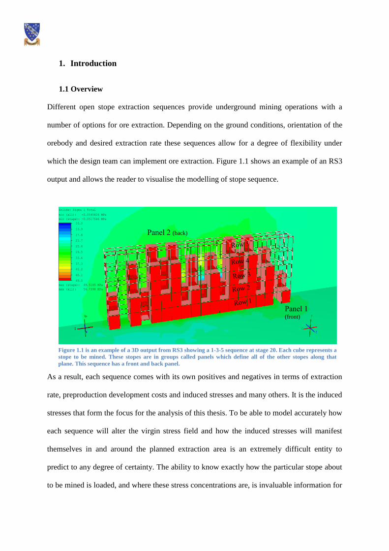
which the design team can implement ore extraction. Figure 1.1 shows an example of an RS3
output and allows the reader to visualise the modelling of stope sequence.
As a result, each sequence comes with its own positives and negatives in terms of extraction
rate, preproduction development costs and induced stresses and many others. It is the induced
stresses that form the focus for the analysis of this thesis. To be able to model accurately how
each sequence will alter the virgin stress field and how the induced stresses will manifest
themselves in and around the planned extraction area is an extremely difficult entity to
predict to any degree of certainty. The ability to know exactly how the particular stope about
to be mined is loaded, and where these stress concentrations are, is invaluable information for
Solids: Sigma 1 Total
10.0
13.9
17.8
21.7
25.6
29.5
33.4
37.3
41.2
45.1
49.0
min (all): -0.0545826 MPa
min (stage): -0.0517546 MPa
max (stage): 49.5185 MPa
max (all): 54.7398 MPa
Figure 1.1 is an example of a 3D output from RS3 showing a 1-3-5 sequence at stage 20. Each cube represents a
stope to be mined. These stopes are in groups called panels which define all of the other stopes along that
plane. This sequence has a front and back panel.
Panel 1 (front)
Panel 2 (back)

2
mine planning. With accurate knowledge of this it can be ensured that the extraction of the
stope can be carried out with minimal dilution/overbreak, optimal fragmentation and at all
times is as safe as reasonably practicable.
1.2 Scope for Thesis
Using Rocscience’s Rock and Soil 3D (RS3) software (Rocscience, 2014), , this thesis aims
to model the different induced stresses and the impact on the rockmass created from four
popular stope sequencing options used in the mining industry . The sequences considered are:
continuous, 1-3-5, 1-4-7 and 1-5-9.
This project examines the following aspects:
1. Compare the sequences in terms of overall damage experienced within critical stopes
2. Damage:
a. Identify and investigate damaged regions unique to each sequence within the stope
block.
b. Ascertain the level of damage within the Hangingwall and Footwall.
3. Assess the sequences with regard to the stage in which the damage begins to occur.
4. Assess the impact of increased depth on the stability of the sequences.
3
2. Sub-Level Open Stoping
The Sub Level Open Stope (SLOS) mining method is a common underground extractive
technique used in metalliferous mines across the mining industry. The SLOS method is used
to extract large massive or tabular, often steeply-dipping competent orebodies surrounded by
competent host rocks which in general have few constraints regarding the shape, size and
continuity of the mineralisation (Villaescusa, 2000).
There are a number of different permutations of the SLOS method, but extraction sequences
are fundamental to achieve production targets safely and economically throughout a mine’s
life. In most underground mines, a number of stopes, in various stages of development,
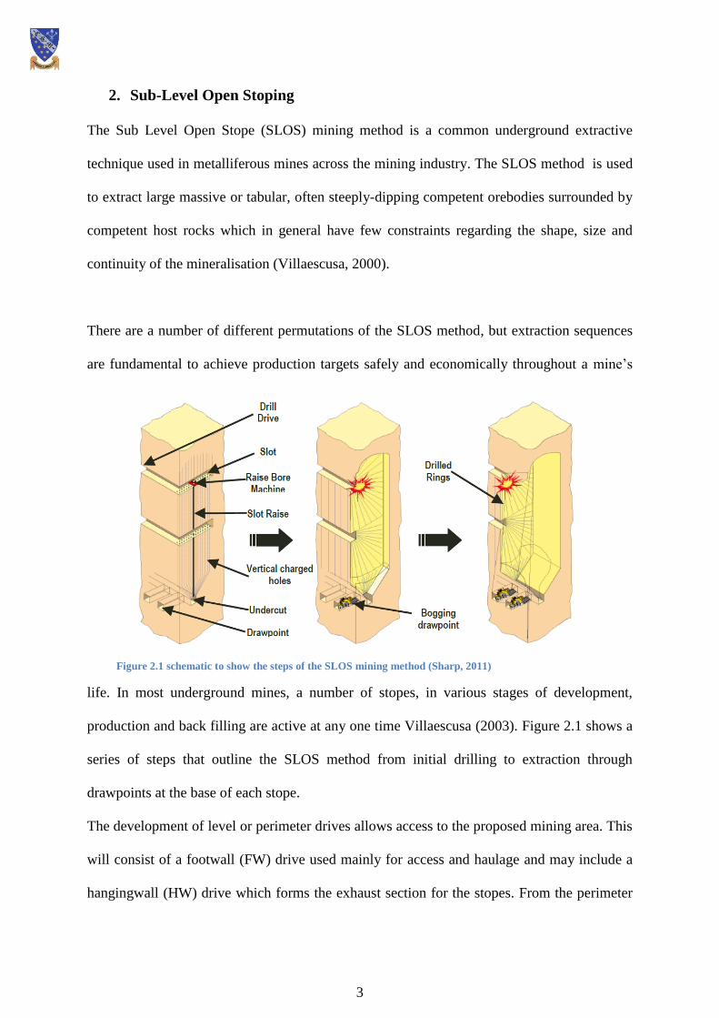
production and back filling are active at any one time Villaescusa (2003). Figure 2.1 shows a
series of steps that outline the SLOS method from initial drilling to extraction through
drawpoints at the base of each stope.
The development of level or perimeter drives allows access to the proposed mining area. This
will consist of a footwall (FW) drive used mainly for access and haulage and may include a
hangingwall (HW) drive which forms the exhaust section for the stopes. From the perimeter
Figure 2.1 schematic to show the steps of the SLOS mining method (Sharp, 2011)

4
drives, cross cuts then provide access to the stope. The slot (Figure 2.1) is then mined from
drill drives inside the area stope. Depending on the height and width of the stope, the amount
of in-stope development per level and number of drill levels will vary. During this stage draw
points on the extraction level, will be constructed from which the blasted, broken ore will be
extracted with a manned or tele-remote loader. Once the blast holes have been drilled and
charged they are progressively blasted and extracted by level.
Stopes can be defined as either primary, secondary, tertiary, or quaternary based on the
number of fill exposures they have:
Primary stopes – no fill exposures all stope walls are rock
Secondary stopes: 1 to 2 walls are fill (depending on the sequence).
Tertiary stopes: 2 – 3 walls are fill.
Quaternary stopes: ≥3 walls are fill.
The Open Stoping method relies on the initial mining of stopes in virgin ore zones (Stephan
1 2 3 4
Decline
Footwall Drive
Cross Cuts
Pendant Pillar
Figure 2.2 shows an idealised stoping sequence for single stopes in a 1-4-7 pattern from Villaescusa (2000) with
conceptual development including a footwall drill drive, decline and cross cuts. The filled stopes in position 1 and
4 are ‘primary’ stopes with 2 a ‘secondary’ and 3 a ‘tertiary’ stope.
5
in SME Handbook, 2011).
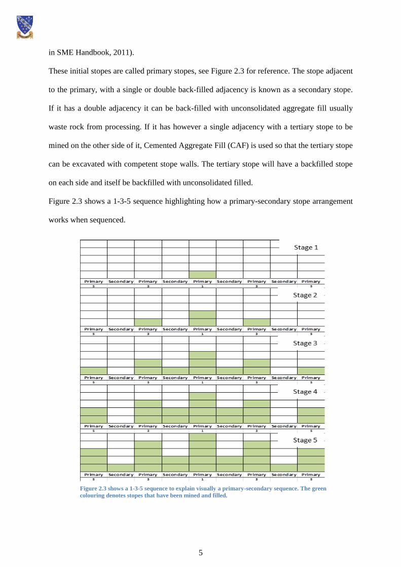
These initial stopes are called primary stopes, see Figure 2.3 for reference. The stope adjacent
to the primary, with a single or double back-filled adjacency is known as a secondary stope.
If it has a double adjacency it can be back-filled with unconsolidated aggregate fill usually
waste rock from processing. If it has however a single adjacency with a tertiary stope to be
mined on the other side of it, Cemented Aggregate Fill (CAF) is used so that the tertiary stope
can be excavated with competent stope walls. The tertiary stope will have a backfilled stope
on each side and itself be backfilled with unconsolidated filled.
Figure 2.3 shows a 1-3-5 sequence highlighting how a primary-secondary stope arrangement
works when sequenced.
Figure 2.3 shows a 1-3-5 sequence to explain visually a primary-secondary sequence. The green
colouring denotes stopes that have been mined and filled.
6
The SLOS method is often chosen because of its low operating costs, the ability to apply
highly mechanised equipment, non-entry production, mobile drilling and loading equipment,
and high production rates with a minimum level of personnel. Conversely the downsides of
the method include a substantial amount of pre-production development requiring substantial
capital investment; stope design requires regular boundaries for ideal extraction; dilution may
occur (waste or backfill material) and the risk of insufficient breakage leading to ore
production losses (Villaescusa 2004).
2.1 Stope Stability, Dimension and Pillar Strength
2.1.1 Stope Stability
Failure of underground openings in hard rock is a function of the in situ stress magnitudes
and the characteristics of the rock mass, i.e., the intact rock strength, major structures such as
faults and the fracture network. At low in situ stress magnitudes, the failure process is
controlled by the continuity and distribution of the natural fractures in the rock mass.
However as in situ stress magnitudes increase, the failure process is dominated by new stress-
induced fractures growing parallel to the excavation boundary (Martin et al, 1999).
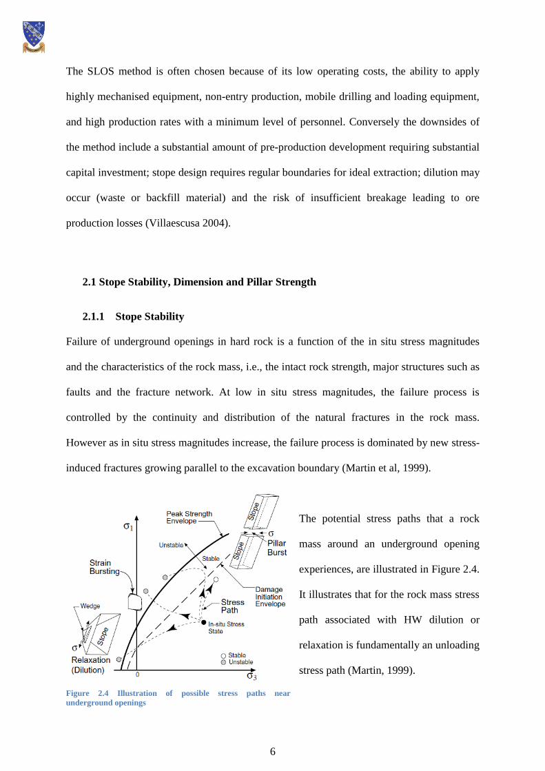
The potential stress paths that a rock
mass around an underground opening
experiences, are illustrated in Figure 2.4.
It illustrates that for the rock mass stress
path associated with HW dilution or
relaxation is fundamentally an unloading
stress path (Martin, 1999).
Figure 2.4 Illustration of possible stress paths near
underground openings
7
It is well known that the behaviour of a jointed rock mass is controlled by the confinement,
e.g., a very blocky hangingwall or tunnel roof will collapse by a process often referred to as
unravelling or slabbing if the confinement is removed. In a good quality rock mass with
discontinuous joints this unravelling will not occur unless new fracture growth occurs.
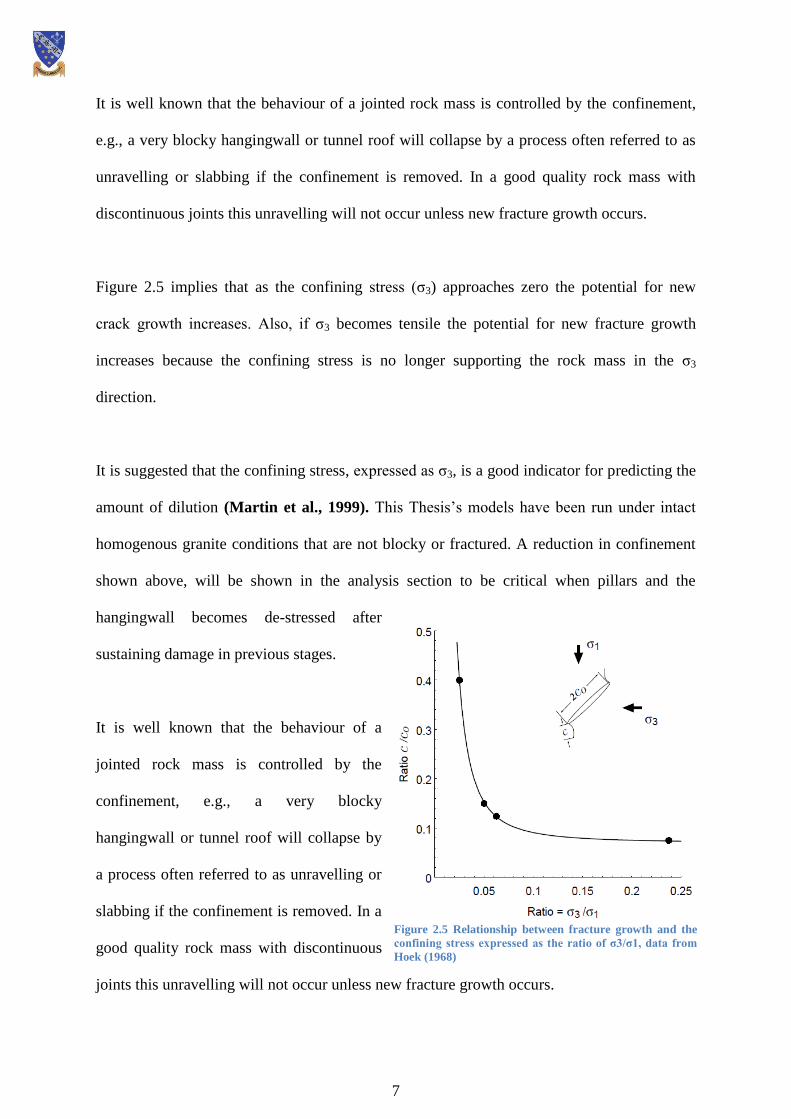
Figure 2.5 implies that as the confining stress (σ3) approaches zero the potential for new
crack growth increases. Also, if σ3 becomes tensile the potential for new fracture growth
increases because the confining stress is no longer supporting the rock mass in the σ3
direction.
It is suggested that the confining stress, expressed as σ3, is a good indicator for predicting the
amount of dilution (Martin et al., 1999). This Thesis’s models have been run under intact
homogenous granite conditions that are not blocky or fractured. A reduction in confinement
shown above, will be shown in the analysis section to be critical when pillars and the
hangingwall becomes de-stressed after
sustaining damage in previous stages.
It is well known that the behaviour of a
jointed rock mass is controlled by the
confinement, e.g., a very blocky
hangingwall or tunnel roof will collapse by
a process often referred to as unravelling or
slabbing if the confinement is removed. In a
good quality rock mass with discontinuous
joints this unravelling will not occur unless new fracture growth occurs.
Figure 2.5 Relationship between fracture growth and the
confining stress expressed as the ratio of σ3/σ1, data from
Hoek (1968)
8
Figure 2.5 implies that as the confining stress (σ3) approaches zero the potential for new
crack growth increases. Also, if σ3 becomes tensile the potential for new fracture growth
increases because the confining stress is no longer supporting the rock mass in the σ3
direction.
It is suggested that the confining stress, expressed as σ3, is a good indicator for predicting the
amount of dilution (Martin et al., 1999) in blocky fractured rock mass condtions. This
Thesis’s models have been run under intact homogenous granite conditions that are not
blocky or fractured and therefore DS will be an effective tool for investigating damage. A
reduction in confinement shown above, will be shown in the analysis section to be critical
when pillars and the hangingwall becomes de-stressed after sustaining damage in previous
stages.
2.1.1.1 Typical Failure Modes in open stopes
The following factors may contribute to failure in open stopes:
- Size and geometry of openings
- Geological features such as folds, joints, faults and shears
- Stress redistribution due to excavations and mining activities
Failure will commonly occur as a result of a combination of these factors. For example when
the size of an opening increases, the possibility of failure for geological or stress reasons also
increases. Most stability problems in stopes are related to discontinuities in the rockmass and
not to the material properties of the rock itself and is therefore more likely to fail along a line
of weakness rather than shear through a competent homogenous block of rock.
Depending on the in situ rock conditions the mode of failure will follow one of these three
failure paths shown in figure 2.6. The OD granite being modelled is most likely to yield in

9
the ‘elastic brittle’ manner
because of its high UCS of
150MPa it will absorb significant
stress before then yielding to a
point of greatly reduced material
strength.
Poole and Mutton (1977) in
Tavakoli (1994) summarised the typical modes of failure in cut-and-fill stoping. Therefore
when damage occurs the types of failure that will occur will include:
1. Longitudinal wedge failure in the back
2. Small wedge failure in the back
3. H/W failure; large vertical exposures of the stope H/W can fail especially when it is
composed of incompetent rock
4. Transverse wedge failure in the back
5. High stress induced failures; ground failure occurs due to high stress concentrations as
a result of mining a number of orebodies simultaneously.
2.1.2 Dimensions
Stope size is vital in terms of production rate and the managing the safety of the working
environment by minimising failures. Dimensions of openings have direct effects on costs
associated with the mucking, haulage, crushing, hoisting, milling, treatment of waste rock
and time to place backfill. Large stopes require more backfill however they have an increased
production rate and require less development. In terms of geotechnics, larger excavations
cause yielding in the surrounding rock which can be detrimental to future mining operation.
Therefore the size and shape of stopes are dictated by the geotechnical conditions of the
Figure 2.6 Post-peak failure characteristics: (a) Very good quality hard
rock mass – Elastic brittle; (b) Average quality rock mass – Stain
softening; (c) Very poor quality soft rock mass – Elastic-plastic.

10
rockmass, the mechanical properties of the planned fill as well as production concerns
(Stephan in SME Handbook, 2011).
Stope size can also be varied between primary and secondary stopes. If the emphasis in the
mine plan is on early tonnage, primary stopes will be wider than secondary stopes if the
ground conditions allow narrower pillars to be stable. If, however, early tonnes are not
essential and the cost of fill is a constraint, the primaries will be narrower and therefore need
less expensive CAF which allows the wider secondaries to be backfilled with unconsolidated
fill reducing costs significantly.
One of the limiting factors affecting the design of an underground excavation is the
maximum void space that a rockmass can sustain without failure. This failure may take place
as a function of either movement along planes of weakness, or through a combination of
intact rock failures and geological discontinuities. In most orebodies suitable to open stoping,
the volume that may be safely excavated, such that stope wall failures are minimised, is many
times smaller than the orebody itself.
Consequently, a series of individual stopes
must be excavated to achieve full orebody
extraction (Villaescusa, 2003). It is then
the sequence in which the series of
individual stopes are extracted that forms
the focus of this thesis.
The Stability Graph Method for stope
design was first introduced by Mathews et
6.25
1.3
16.7
Figure 2.7 shows the modified Mathews stability graph with
N’ values for crown and wall values of 1.3 and 16.7 from
Sharp (2011) plotted against a Hydraulic Radius based on a
25mx25mx30m stope of 6.25m.

11
al. in 1981 and later modified by Potvin et al. (1989). The current version of the method,
based on the analysis of more than 350 case histories collected from Canadian hard rock
underground mines, is widely used as the first step in the stope design process (Fig. 5). The
stability number N is defined as:
Where Q’ is the modified Q Tunnelling Quality Index (Bieniawski, 1989); A is the rock
stress factor; B is the joint orientation adjustment factor; and C is the gravity adjustment
factor. The modified Tunnelling Quality Index Q is determined from the structural mapping
of the rock mass and for this thesis is 6.3 for the crown and 8.3 for the walls. However it is
important to bear in mind that the Stability Graph Method does not consider the effect of
confining stress and so should be taken as a way of determining rough stable stope
dimension.
2.1.3 Pillar Stability
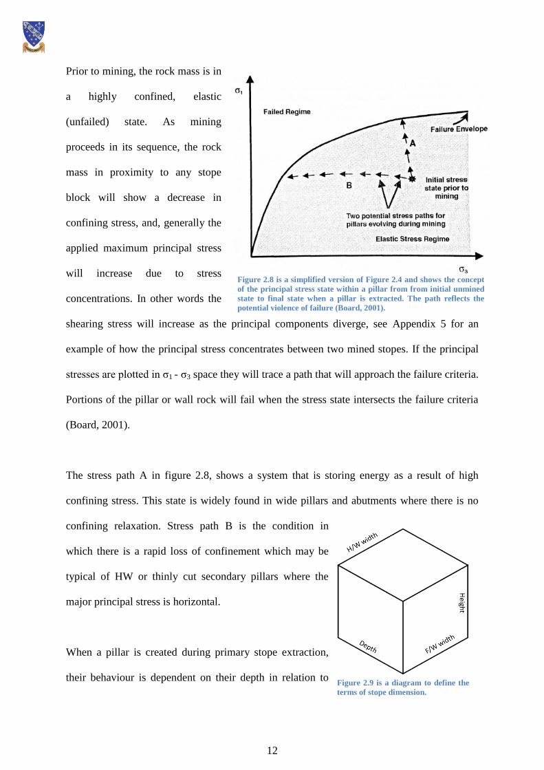
Prior to mining, the rock mass is in a highly confined, elastic (unfailed) state. As mining
proceeds in its sequence, the rock mass in proximity to any stope block will show a decrease
in confining stress, and, generally the applied maximum principal stress will increase due to
stress concentrations. In other words the shearing stress will increase as the principal
components diverge, see Appendix 5 for an example of how the principal stress concentrates
between two mined stopes. If the principal stresses are plotted in s1-s3 space they will trace a
path that will approach the failure criteria. Portions of the pillar or wall rock will fail when
the stress state intersects the failure criteria (Board, 2001).
12
Prior to mining, the rock mass is in
a highly confined, elastic
(unfailed) state. As mining
proceeds in its sequence, the rock
mass in proximity to any stope
block will show a decrease in
confining stress, and, generally the
applied maximum principal stress
will increase due to stress
concentrations. In other words the
shearing stress will increase as the principal components diverge, see Appendix 5 for an
example of how the principal stress concentrates between two mined stopes. If the principal
stresses are plotted in σ1 - σ3 space they will trace a path that will approach the failure criteria.
Portions of the pillar or wall rock will fail when the stress state intersects the failure criteria
(Board, 2001).
The stress path A in figure 2.8, shows a system that is storing energy as a result of high
confining stress. This state is widely found in wide pillars and abutments where there is no
confining relaxation. Stress path B is the condition in
which there is a rapid loss of confinement which may be
typical of HW or thinly cut secondary pillars where the
major principal stress is horizontal.
When a pillar is created during primary stope extraction,
their behaviour is dependent on their depth in relation to
Figure 2.8 is a simplified version of Figure 2.4 and shows the concept
of the principal stress state within a pillar from from initial unmined
state to final state when a pillar is extracted. The path reflects the
potential violence of failure (Board, 2001).
Figure 2.9 is a diagram to define the
terms of stope dimension.
13
their HW to FW width (Figure 2.9). A 15m wide pillar for example tends to fail by following
a stress path that achieves the failure criteria through low confinement as opposed to high
stress build up. As a result there is a non-violent shear failure because the principal stresses
redistribute into the abutments which has little impact on the mining process. This behaviour
is somewhere between A and B in Figure 2.8. A 30m pillar on the other hand completely
changes stope behaviour. Because this pillar’s stress path follows A in Figure 2.8, the level of
confinement remains high and therefore a highly stressed, elastic pillar core. Seismicity had
been experienced with the use of 30m secondaries because the confinement remains high
until failure whereupon there is a violent reaction (Board, 2001).
2.2 Review of Different Sequence Options
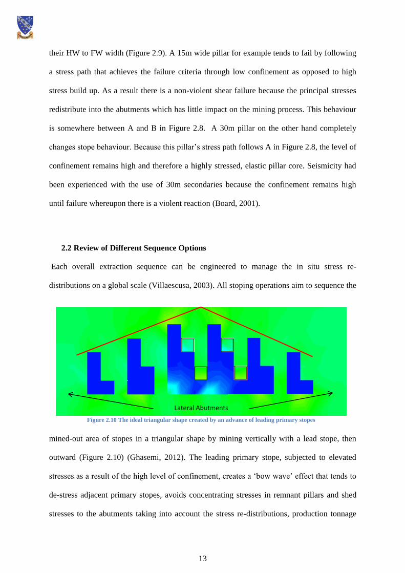
Each overall extraction sequence can be engineered to manage the in situ stress re-
distributions on a global scale (Villaescusa, 2003). All stoping operations aim to sequence the
mined-out area of stopes in a triangular shape by mining vertically with a lead stope, then
outward (Figure 2.10) (Ghasemi, 2012). The leading primary stope, subjected to elevated
stresses as a result of the high level of confinement, creates a ‘bow wave’ effect that tends to
de-stress adjacent primary stopes, avoids concentrating stresses in remnant pillars and shed
stresses to the abutments taking into account the stress re-distributions, production tonnage
Lateral Abutments
Figure 2.10 The ideal triangular shape created by an advance of leading primary stopes
14
requirements and access constraints (Board et al., 2001, Potvin and Hudyma, 2000,
Villaescusa, 2003). As a general rule, primary stopes are usually mined and filled two vertical
lifts before the mining of secondary stopes commences.
2.2.1 Top Down or Bottom Up
A decision must be made as to whether the mining sequence will be top-down or bottom-up.
There are a number of operational, scheduling and economic reasons for mining an orebody
from bottom to top. From a geotechnical point of view, bottom up mining can be an effective
means of stress management.
When mining in high stress conditions, extraction ideally progresses from the bottom to top.
As the total extraction increases and the stress concentrates, the extraction horizon moves
towards the shallower levels of the mine and towards the areas of lower premining stresses.
As a result, high induced stresses and deteriorating ground conditions are better managed.
Ultimately, it will minimise stress related problems as extraction progresses and the backfill
will be used as a floor to work on in a ‘short’ lift, bottom-up mining sequence (Potvin &
Hudyma, 2000).
This Thesis’s modelling will be run on the assumption that mining will be bottom-up.
The main four permutations of the Open Stoping method are listed below.
Continuous – Pyramidal
1-3-5 – Primary-Secondary
1-4-7 – Primary-Secondary-Tertiary
1-5-9 – Primary-Secondary-Tertiary

15
2.2.2 Continuous Sequence
The ideal stress management stoping sequence is a systematic retreat from the centre-out,
without pillars, progressing with the triangular shape shown in figure 2.11. Although a
continuous advancing stoping sequence is an attractive idea in terms of total recovery, it is
very hard to implement, especially when stopes are backfilled in the sequence. Because each
individual stope must be mined, filled and cured before an adjacent stope can be extracted,
productivity is constrained by the individual stope cycle times. A pillarless stoping sequence
requires rapidly curing cemented backfill with minimal drainage delays in all the stopes,
which may increase the operating cost (Ghasemi, 2012).
Figure 2.11 Centre-out, continuous pattern (Ghasemi, 2012)
16
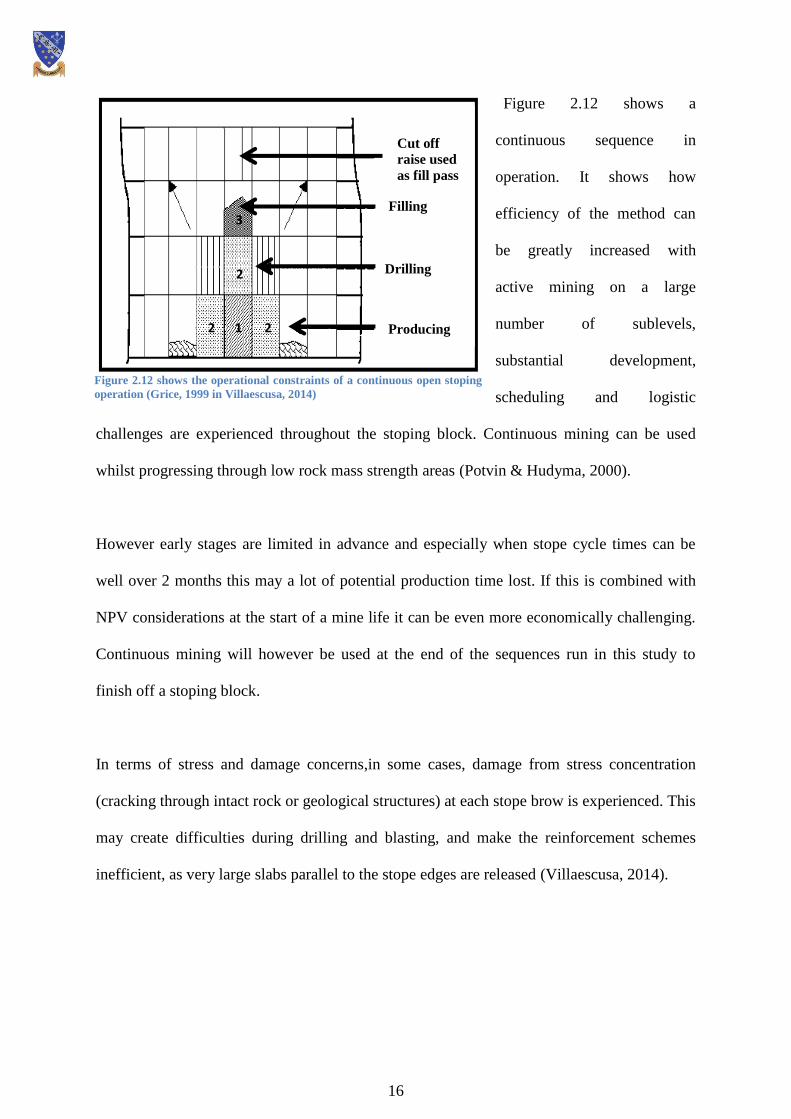
Figure 2.12 shows a
continuous sequence in
operation. It shows how
efficiency of the method can
be greatly increased with
active mining on a large
number of sublevels,
substantial development,
scheduling and logistic
challenges are experienced throughout the stoping block. Continuous mining can be used
whilst progressing through low rock mass strength areas (Potvin & Hudyma, 2000).
However early stages are limited in advance and especially when stope cycle times can be
well over 2 months this may a lot of potential production time lost. If this is combined with
NPV considerations at the start of a mine life it can be even more economically challenging.
Continuous mining will however be used at the end of the sequences run in this study to
finish off a stoping block.
In terms of stress and damage concerns,in some cases, damage from stress concentration
(cracking through intact rock or geological structures) at each stope brow is experienced. This
may create difficulties during drilling and blasting, and make the reinforcement schemes
inefficient, as very large slabs parallel to the stope edges are released (Villaescusa, 2014).
1
2
3
2 2
Cut off
raise used
as fill pass
Filling
Drilling
Producing
Figure 2.12 shows the operational constraints of a continuous open stoping
operation (Grice, 1999 in Villaescusa, 2014)
17
2.2.3 Primary-Secondary
Massive orebodies can be extracted using multiple stopes (primary, secondary and when
required tertiary) in conjunction with mass blasting techniques and cemented fill. A number
of sequencing options can be used including temporary rib, crown and transverse pillars. This
thesis however will not make use of these types of pillars in the modelling. The only pillars
that will be used will be planned stopes (which act as temporary ribs).
The advantages of the primary and secondary stoping sequences lie in the initial high
flexibility, productivity and low cost during primary stoping. The overall cost is minimised
by the use of unconsolidated fill within the secondary stopes. A negative aspect of the
primary-secondary method is induced stress re-distributions may cause rock mass damage
within secondary pillars in the extraction sequence (Ghasemi, 2012). This problem can be
mitigated by avoiding undercutting of individual stopes and by mass blasting those localised
regions of high stress within the stoping block. Multiple lift primary and secondary stopes
have been used very successfully to achieve complete extraction with minimal dilution within
the steeply dipping lead orebodies at Mount Isa Mines (Bywater et al, 1985).
18
2.2.4 Stoping Sequence 1-3-5
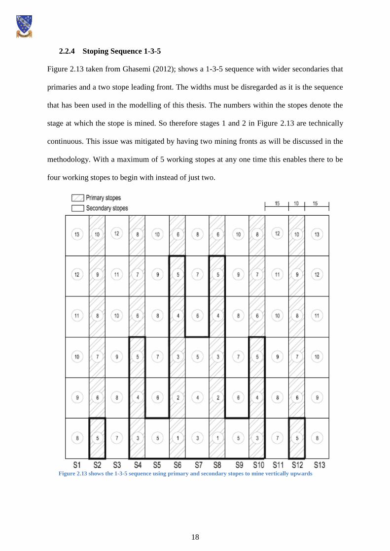
Figure 2.13 taken from Ghasemi (2012); shows a 1-3-5 sequence with wider secondaries that
primaries and a two stope leading front. The widths must be disregarded as it is the sequence
that has been used in the modelling of this thesis. The numbers within the stopes denote the
stage at which the stope is mined. So therefore stages 1 and 2 in Figure 2.13 are technically
continuous. This issue was mitigated by having two mining fronts as will be discussed in the
methodology. With a maximum of 5 working stopes at any one time this enables there to be
four working stopes to begin with instead of just two.
Figure 2.13 shows the 1-3-5 sequence using primary and secondary stopes to mine vertically upwards
19
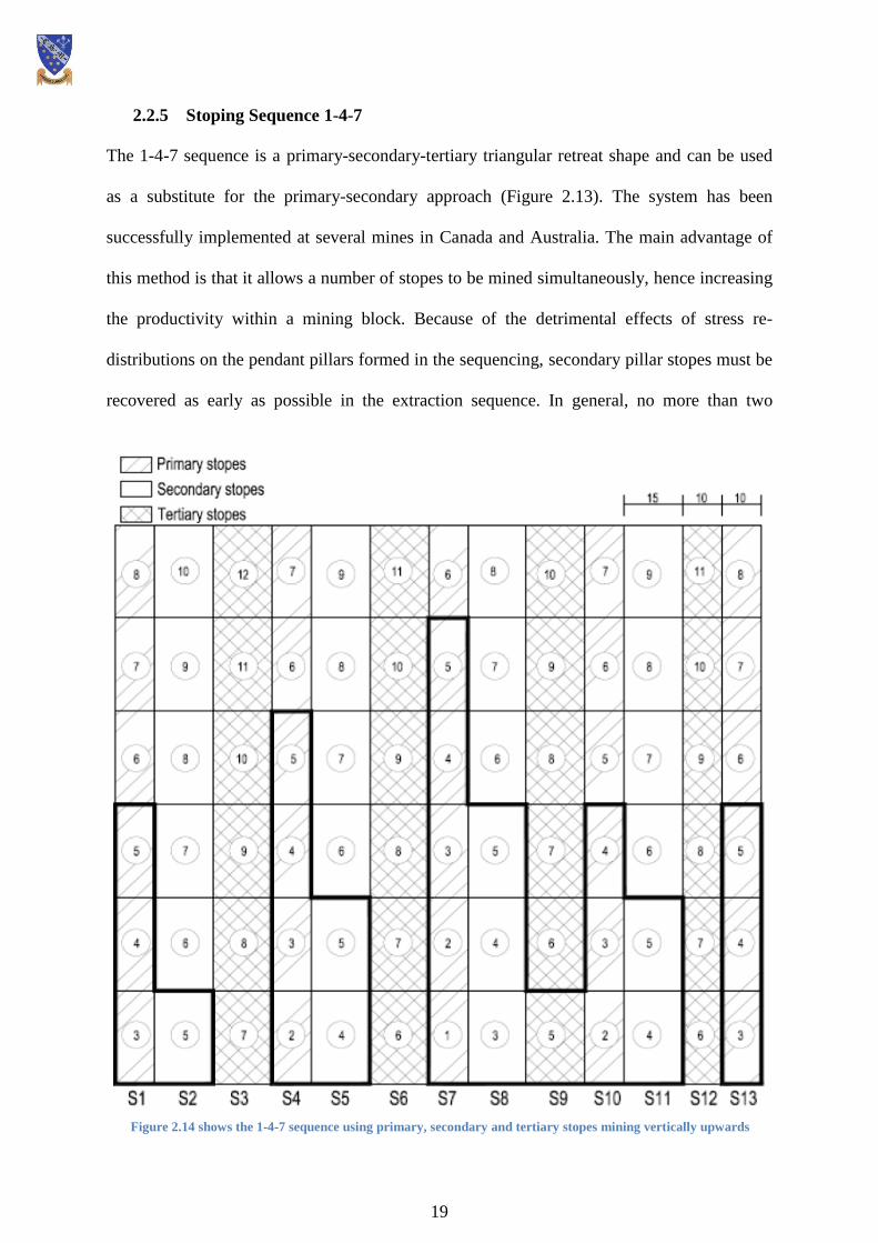
2.2.5 Stoping Sequence 1-4-7
The 1-4-7 sequence is a primary-secondary-tertiary triangular retreat shape and can be used
as a substitute for the primary-secondary approach (Figure 2.13). The system has been
successfully implemented at several mines in Canada and Australia. The main advantage of
this method is that it allows a number of stopes to be mined simultaneously, hence increasing
the productivity within a mining block. Because of the detrimental effects of stress re-
distributions on the pendant pillars formed in the sequencing, secondary pillar stopes must be
recovered as early as possible in the extraction sequence. In general, no more than two
Figure 2.14 shows the 1-4-7 sequence using primary, secondary and tertiary stopes mining vertically upwards
20
sublevels are mined ahead of a pillar before recovering it and both sides of a pillar cannot be
mined simultaneously (Potvin and Hudyma, 2000).
The main problem with this method is that the sequencing should be followed strictly during
the entire extraction process or else bursting in pillars rather than gradual failing can be
expected (Ghasemi, 2012). Moreover this method sees a rise in the expense of fill material
given that both primary and secondary stopes must be backfilled with cemented fill with only
tertiary stopes being backfilled with waste material fill.
21
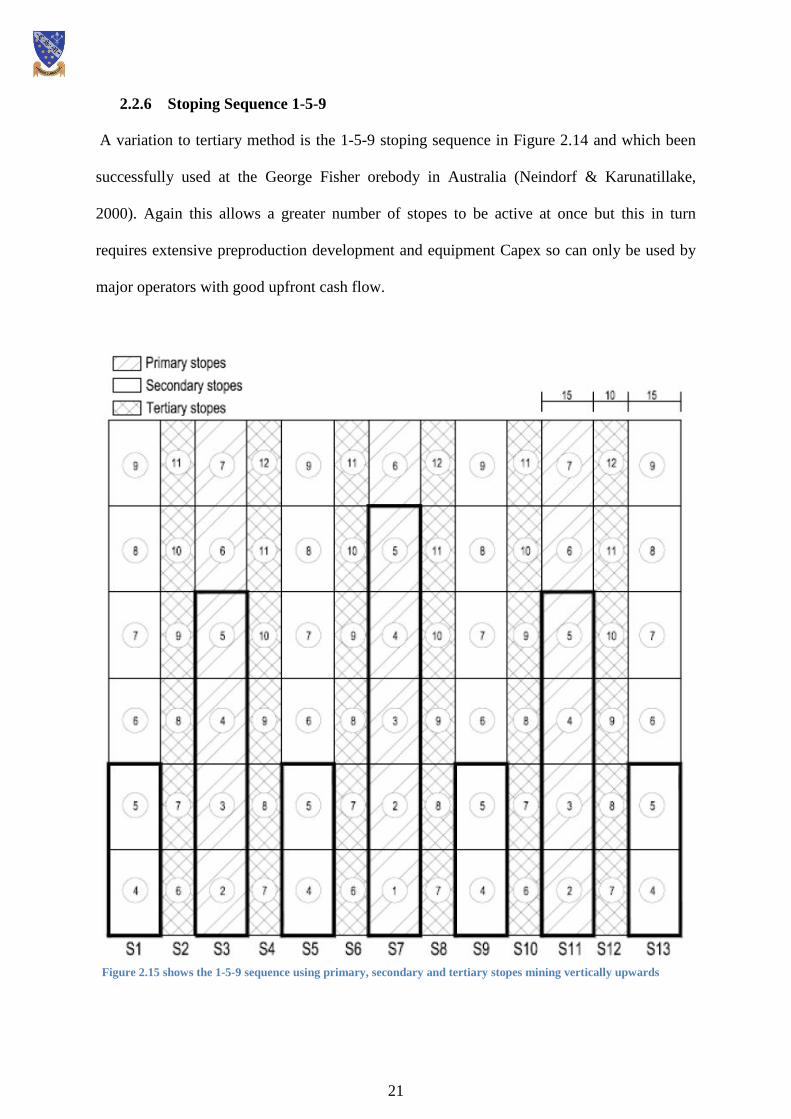
2.2.6 Stoping Sequence 1-5-9
A variation to tertiary method is the 1-5-9 stoping sequence in Figure 2.14 and which been
successfully used at the George Fisher orebody in Australia (Neindorf & Karunatillake,
2000). Again this allows a greater number of stopes to be active at once but this in turn
requires extensive preproduction development and equipment Capex so can only be used by
major operators with good upfront cash flow.
Figure 2.15 shows the 1-5-9 sequence using primary, secondary and tertiary stopes mining vertically upwards
22
A disadvantage of a 1-5-9 (or 1-4-7) extraction sequence using short lift stopes is their
inefficient stope mucking characteristics. The method effectively requires (a bottom up)
moving drawpoint sequence (even in primary stopes), which necessarily follows the vertical
retreat of the stopes. This implies that mucking is carried out in areas that had previously
been subjected to stress distribution and stope blasting at the stope crowns. Each stope access
becomes a stope drawpoint and a significant amount of reinforcement using cablebolting is
required in all the stopes access and exposed backs. Reinforcement can be largely inefficient
within the bottom of pendant secondary pillars ( also true for 1-3-5) where remote mucking is
required for 100% of the tonnage. Furthermore, additional FW development access in waste
may be required on each sublevel, as more than one access may be required for effective
mucking of each individual stope (Ghasemi, 2012).
3. Olympic Dam Background
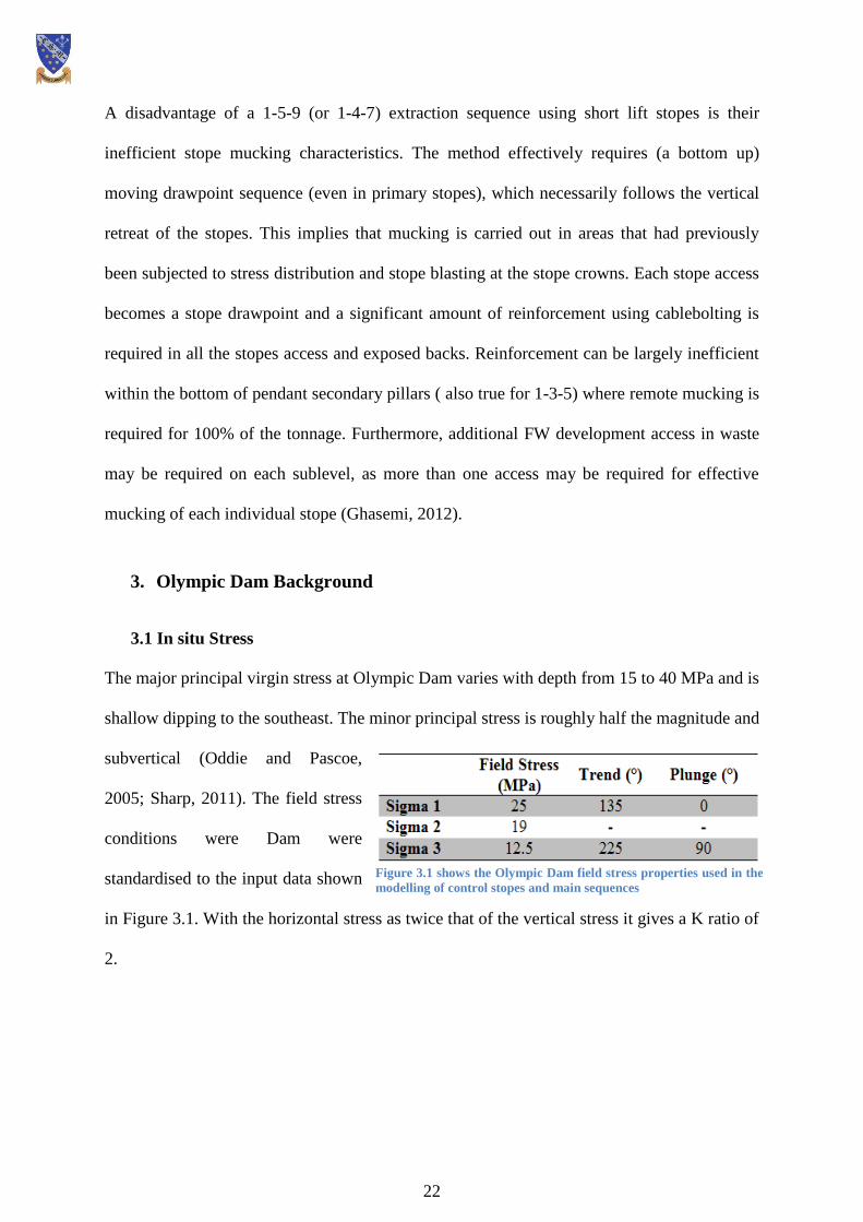
3.1 In situ Stress
The major principal virgin stress at Olympic Dam varies with depth from 15 to 40 MPa and is
shallow dipping to the southeast. The minor principal stress is roughly half the magnitude and
subvertical (Oddie and Pascoe,
2005; Sharp, 2011). The field stress
conditions were Dam were
standardised to the input data shown
in Figure 3.1. With the horizontal stress as twice that of the vertical stress it gives a K ratio of
2.
Figure 3.1 shows the Olympic Dam field stress properties used in the
modelling of control stopes and main sequences
23
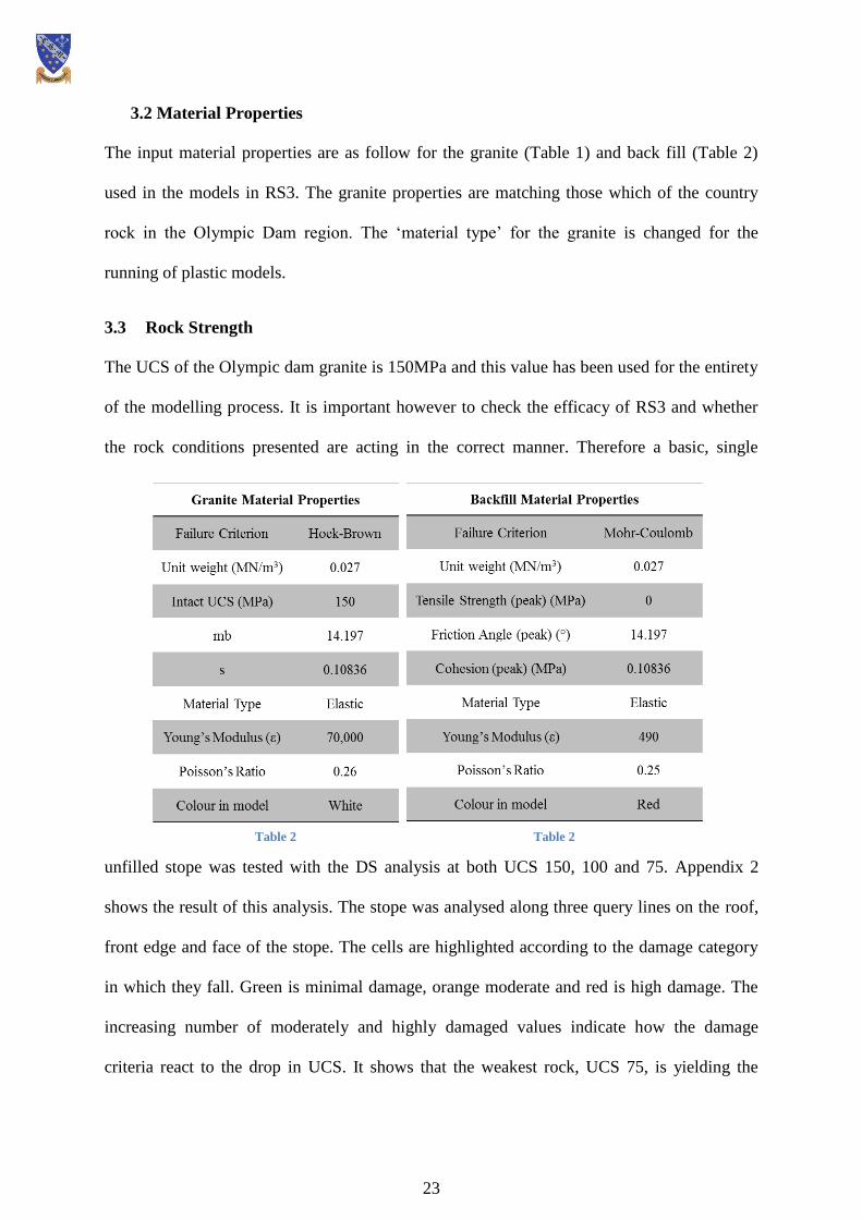
3.2 Material Properties
The input material properties are as follow for the granite (Table 1) and back fill (Table 2)
used in the models in RS3. The granite properties are matching those which of the country
rock in the Olympic Dam region. The ‘material type’ for the granite is changed for the
running of plastic models.
3.3 Rock Strength
The UCS of the Olympic dam granite is 150MPa and this value has been used for the entirety
of the modelling process. It is important however to check the efficacy of RS3 and whether
the rock conditions presented are acting in the correct manner. Therefore a basic, single
unfilled stope was tested with the DS analysis at both UCS 150, 100 and 75. Appendix 2
shows the result of this analysis. The stope was analysed along three query lines on the roof,
front edge and face of the stope. The cells are highlighted according to the damage category
in which they fall. Green is minimal damage, orange moderate and red is high damage. The
increasing number of moderately and highly damaged values indicate how the damage
criteria react to the drop in UCS. It shows that the weakest rock, UCS 75, is yielding the
Table 2 Table 2
24
most, in line with the expectation of the model’s results.
3.4 Dimension
An appropriate stable standard dimension was crucial to fix upon before beginning the
analysis. Three different dimensions were tested. Stope height and depth were fixed at 30m
and 25m respectively with just the span being flexed. The width to height ratio in the pillars
must not exceed a critical threshold as shown in Appendix 3. A low width to height ratio
ensures the pillars have enough structural strength to remain intact under high stress
The three spans tested were 15m, 20m and 25m. The main principal stress runs at 135° to the
stope so therefore the greatest stress is not vertical which would be the orientation at which
these pillars would be most vulnerable. Both the pillar strength as well as roof strength is
considered because the excavation must remain intact when unsupported. The dimension will
be tested using DS as a way of indicating the likelihood of damage or yield. This analysis will
use percentages for this analysis, so therefore 0.2 will be represented as 20%. The ‘max’
values are not referenced as they only illustrate the extremes from which to standardise the
other results.
Appendix 3 shows the three variations under σ1 and σ3 total analysis. The stress conditions
are uniform with 25MPa of in situ stress running perpendicular to the main face in each
model. As Appendix 3 shows, the stress contours around the excavation changes with the
different analysed stress. With the 15m stope under σ1 analysis the stressed contour in the
roof is much more pronounced than in the 20m and 25m. This could lead to damage from
change in stress upon the mining of subsequent stopes but under single stope analysis the DS
is shown in the roof to be at a maximum of 18% (σ1 of 40.2MPa, σ3 of 13.4MPa) which is
minimal damage. A similar result can be found for the front of the excavation at 15m width

25
with a maximum value of 23%.
The 20m variation has a highest value of 27% of UCS which is moderately damaged (σ1 of
55.7MPa, σ3 of 14.9MPa) on the corner, mid-way up the stope. The 25m stope span model
has the highest DS of 32% UCS (σ1 of 48.4MPa, σ3 of 0.7MPa) in the roof section. Whilst
this is not the highest stress found at 48.4 it is the difference with the σ1 value that makes it
significant. With low confining stress this region may be prone to yield. This is however a
minor threat given that this is the worst section of an otherwise stable stope. It can therefore
be concluded that the 25m stope is stable and can be utilised for the stock stope width for
future models. Width to height ratio is almost 1:1 at 0.83:1 and will stand up after excavation.
The control stope dimensions were concluded as stable at 25m x 25m x 30m after varying
base area the excavation was concluded as stable in competent granite UCS of 150MPa under
Hoek-Brown failure criterion. The meshing run for the singular stopes will be run with 100
edges on excavation boundary however 600 edges will be used to model the sequence in the
actual analysis.
26
4. Methodology – Numerical Modelling of Stope Sequences
Four sequencing patterns with identical stope dimensions were studied using primary-
secondary strategy to identify the optimum induced stress permutations of each sequence in
terms of damage and stress concentration. For this purpose, an orebody of 375 meters width,
50 meters strike length and height of 150 meters was modelled and stopes were excavated
according to each pattern, separately. The height of excavation in all the patterns was
restricted to 30 meters and the width and strike length were set at 25m each. Therefore there
were two panels of stopes each 25m in strike length called Panel 1 (FW side) and Panel 2
(HW side). This study is not a comparison of stope dimensions but one of optimum sequence
in terms of stress management. However, section 2.1.2 will demonstrate how a stable stope
dimension was found, suitable for the modelling of an orebody of this size. A stock stope size
was important to model so as to standardise the induced stress result.
4.1 Numerical Modelling
The modelling was done using Rocscience’s Rock and Soil 3D or RS3. RS3 is a general
purpose finite element analysis program for underground excavations (Rocscience, 2014).
Numerical models for underground. Numerical modelling for the analysis of stress driven
problems in rock mechanics can be divided into two classes, boundary methods and domain
methods. The models were run under the domain method; this is where the interior of the
rock mass is divided into geometrically simple elements each with assumed properties. The
collective behaviour and interaction of these simplified elements model the more complex
overall behaviour of the rock mass. Finite element and finite difference are domain methods
that treat the rock mass as a continuum and distinct element method models each individual
block of rock as a unique element (Hoek and Kaiser, 2000).
27
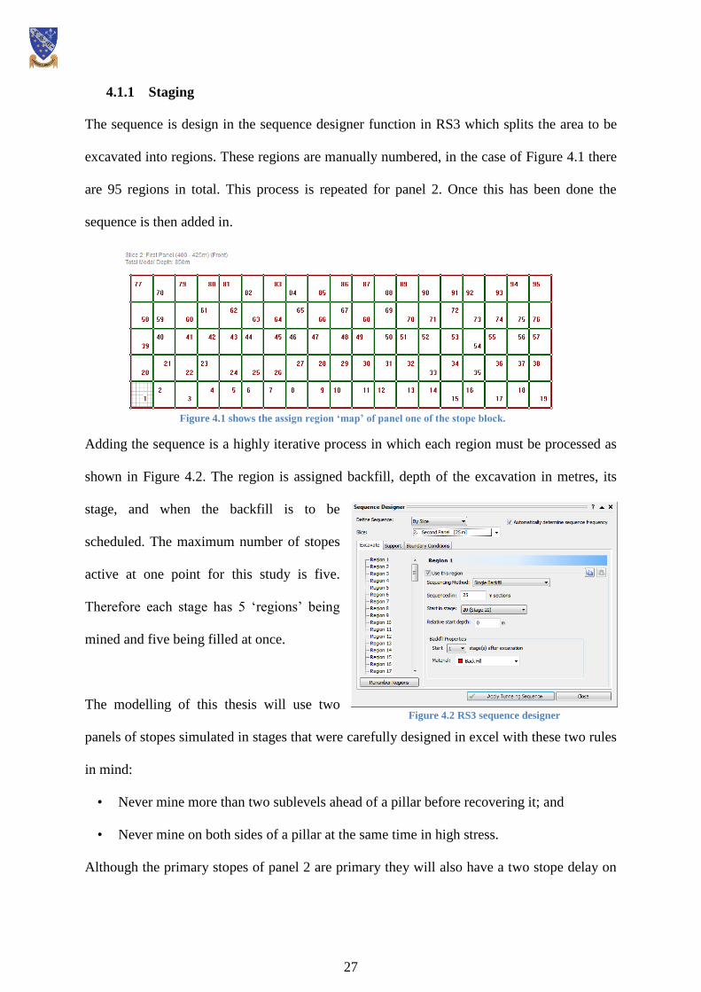
4.1.1 Staging
The sequence is design in the sequence designer function in RS3 which splits the area to be
excavated into regions. These regions are manually numbered, in the case of Figure 4.1 there
are 95 regions in total. This process is repeated for panel 2. Once this has been done the
sequence is then added in.
Adding the sequence is a highly iterative process in which each region must be processed as
shown in Figure 4.2. The region is assigned backfill, depth of the excavation in metres, its
stage, and when the backfill is to be
scheduled. The maximum number of stopes
active at one point for this study is five.
Therefore each stage has 5 ‘regions’ being
mined and five being filled at once.
The modelling of this thesis will use two
panels of stopes simulated in stages that were carefully designed in excel with these two rules
in mind:
• Never mine more than two sublevels ahead of a pillar before recovering it; and
• Never mine on both sides of a pillar at the same time in high stress.
Although the primary stopes of panel 2 are primary they will also have a two stope delay on
Figure 4.1 shows the assign region ‘map’ of panel one of the stope block.
Figure 4.2 RS3 sequence designer
28
the vertical advance of panel 1. This will not always be the case, often reducing to a one stope
delay; however the front and back panels will never be level. Each stage from every sequence
can be seen in the Digital Appendices 1.1-1.4, which shows how the sequence is
implemented in panel 1 and 2. It is imperative that each region is assigned its specific stage
number.
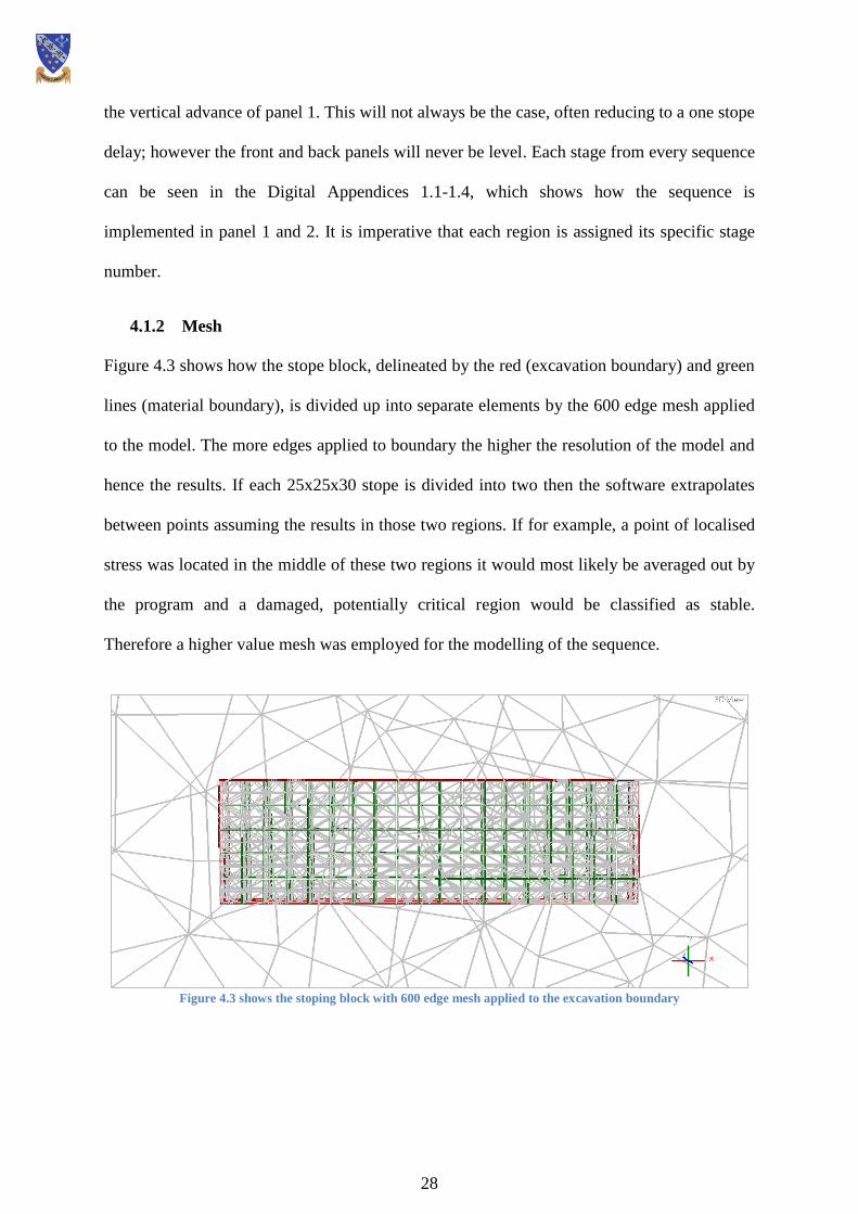
4.1.2 Mesh
Figure 4.3 shows how the stope block, delineated by the red (excavation boundary) and green
lines (material boundary), is divided up into separate elements by the 600 edge mesh applied
to the model. The more edges applied to boundary the higher the resolution of the model and
hence the results. If each 25x25x30 stope is divided into two then the software extrapolates
between points assuming the results in those two regions. If for example, a point of localised
stress was located in the middle of these two regions it would most likely be averaged out by
the program and a damaged, potentially critical region would be classified as stable.
Therefore a higher value mesh was employed for the modelling of the sequence.
Figure 4.3 shows the stoping block with 600 edge mesh applied to the excavation boundary
29
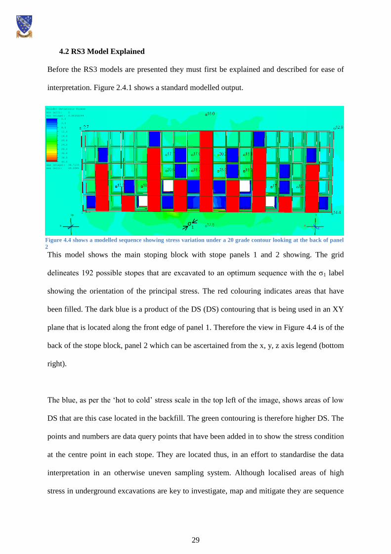
4.2 RS3 Model Explained
Before the RS3 models are presented they must first be explained and described for ease of
interpretation. Figure 2.4.1 shows a standard modelled output.
This model shows the main stoping block with stope panels 1 and 2 showing. The grid
delineates 192 possible stopes that are excavated to an optimum sequence with the σ1 label
showing the orientation of the principal stress. The red colouring indicates areas that have
been filled. The dark blue is a product of the DS (DS) contouring that is being used in an XY
plane that is located along the front edge of panel 1. Therefore the view in Figure 4.4 is of the
back of the stope block, panel 2 which can be ascertained from the x, y, z axis legend (bottom
right).
The blue, as per the ‘hot to cold’ stress scale in the top left of the image, shows areas of low
DS that are this case located in the backfill. The green contouring is therefore higher DS. The
points and numbers are data query points that have been added in to show the stress condition
at the centre point in each stope. They are located thus, in an effort to standardise the data
interpretation in an otherwise uneven sampling system. Although localised areas of high
stress in underground excavations are key to investigate, map and mitigate they are sequence
Solids: Deviatoric Stress
0.0
4.0
8.0
12.0
16.0
20.0
24.0
28.0
32.0
36.0
40.0
min (all): 0
min (stage): 0.00102299
max (stage): 38.7133
max (all): 49.5085
σ1
Figure 4.4 shows a modelled sequence showing stress variation under a 20 grade contour looking at the back of panel
2
30
specific and therefore not a feature that can be compared across sequences. These areas of
particularly high stress will be mapped and noted so they are not disregarded in the analysis.
Another feature that is not included in this graphic is an XZ plane. This when used will show
the stress conditions extending out in the HW or FW depending on the analysis.
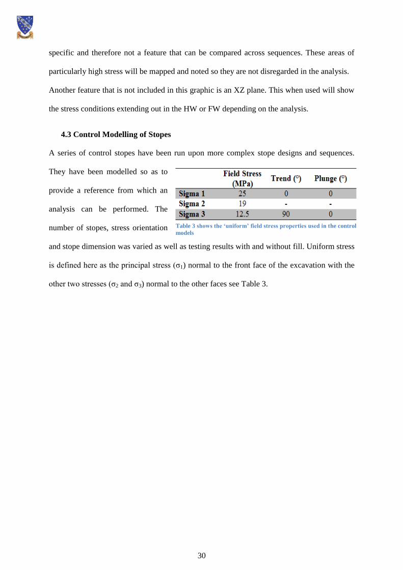
4.3 Control Modelling of Stopes
A series of control stopes have been run upon more complex stope designs and sequences.
They have been modelled so as to
provide a reference from which an
analysis can be performed. The
number of stopes, stress orientation
and stope dimension was varied as well as testing results with and without fill. Uniform stress
is defined here as the principal stress (σ1) normal to the front face of the excavation with the
other two stresses (σ2 and σ3) normal to the other faces see Table 3.
Table 3 shows the ‘uniform’ field stress properties used in the control
models

31
4.4 Different sequencing methods:
4.4.1 Continuous
The continuous sequence uses the sequence taken from Ghasemi (2012) in Figure 2.11. The
first four stages of the sequence with a maximum of five working stopes, begins as is shown
in Figure 4.5. These tables are used with Figure 2.11 to assign a region with a stage. So
therefore in stage 1, stopes 3, 10 and 17 are extracted. In stage 2, stopes 6, 13, 22, 29, 36 are
mined and so on. It only shows panel 1 for stages 1-3 because the front panel’s advance must
be two stopes high before stopes can start being excavated in panel 2. After stage 4 the
sequence carries on, see digital Appendix 1.1
0 0 0 0 0 0 0 0 0 0 0 0 0 0 0 0 0 0 0
0 0 0 0 0 0 0 0 0 0 0 0 0 0 0 0 0 0 0
0 0 0 0 0 0 0 0 0 0 0 0 0 0 0 0 0 0 0
0 0 0 0 0 0 0 0 0 0 0 0 0 0 0 0 0 0 0
0 0 1 0 0 0 0 0 0 1 0 0 0 0 0 0 1 0 0
1 2 3 4 5 6 7 8 9 10 11 12 13 14 15 16 17 18 19
0 0 0 0 0 0 0 0 0 0 0 0 0 0 0 0 0 0 0
0 0 0 0 0 0 0 0 0 0 0 0 0 0 0 0 0 0 0
0 0 0 0 0 0 0 0 0 0 0 0 0 0 0 0 0 0 0
0 0 1 0 0 0 0 0 0 1 0 0 0 0 0 0 1 0 0
0 0 1 0 0 1 0 0 0 1 0 0 1 0 0 0 1 0 0
1 2 3 4 5 6 7 8 9 10 11 12 13 14 15 16 17 18 19
0 0 0 0 0 0 0 0 0 0 0 0 0 0 0 0 0 0 0
0 0 0 0 0 0 0 0 0 0 0 0 0 0 0 0 0 0 0
0 0 0 0 0 0 0 0 0 0 0 0 0 0 0 0 0 0 0
0 0 1 0 0 1 0 0 0 1 0 0 0 0 0 0 1 0 0
0 1 1 1 0 1 0 0 1 1 1 0 1 0 0 0 1 0 0
1 2 3 4 5 6 7 8 9 10 11 12 13 14 15 16 17 18 19
0 0 0 0 0 0 0 0 0 0 0 0 0 0 0 0 0 0 0
0 0 0 0 0 0 0 0 0 0 0 0 0 0 0 0 0 0 0
0 0 0 0 0 0 0 0 0 0 0 0 0 0 0 0 0 0 0
0 0 1 0 0 1 0 0 0 1 0 0 1 0 0 0 1 0 0
0 1 1 1 0 1 0 0 1 1 1 0 1 0 0 1 1 1 0
1 2 3 4 5 6 7 8 9 10 11 12 13 14 15 16 17 18 19
Stage 1
Stage 2
Stage 4 – Panel 1
Stage 3
0 0 0 0 0 0 0 0 0 0 0 0 0 0 0 0 0 0 0
0 0 0 0 0 0 0 0 0 0 0 0 0 0 0 0 0 0 0
0 0 0 0 0 0 0 0 0 0 0 0 0 0 0 0 0 0 0
0 0 0 0 0 0 0 0 0 0 0 0 0 0 0 0 0 0 0
0 0 1 0 0 0 0 0 0 1 0 0 0 0 0 0 1 0 0
1 2 3 4 5 6 7 8 9 10 11 12 13 14 15 16 17 18 19
Stage 4 – Panel 2
Figure 4.5 shows the first 4 stages of the continuous sequence. The black colouring indicates areas that have been
excavated. Stope shape not to scale.
32
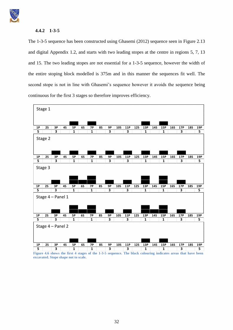
4.4.2 1-3-5
The 1-3-5 sequence has been constructed using Ghasemi (2012) sequence seen in Figure 2.13
and digital Appendix 1.2, and starts with two leading stopes at the centre in regions 5, 7, 13
and 15. The two leading stopes are not essential for a 1-3-5 sequence, however the width of
the entire stoping block modelled is 375m and in this manner the sequences fit well. The
second stope is not in line with Ghasemi’s sequence however it avoids the sequence being
continuous for the first 3 stages so therefore improves efficiency.
Figure 4.6 shows the first 4 stages of the 1-3-5 sequence. The black colouring indicates areas that have been
excavated. Stope shape not to scale.
0 0 0 0 0 0 0 0 0 0 0 0 0 0 0 0 0 0 0
0 0 0 0 0 0 0 0 0 0 0 0 0 0 0 0 0 0 0
0 0 0 0 0 0 0 0 0 0 0 0 0 0 0 0 0 0 0
0 0 0 0 0 0 0 0 0 0 0 0 0 0 0 0 0 0 0
0 0 0 0 1 0 1 0 0 0 0 0 1 0 1 0 0 0 0
1P 2S 3P 4S 5P 6S 7P 8S 9P 10S 11P 12S 13P 14S 15P 16S 17P 18S 19P5 3 1 1 3 3 1 1 3 50 0 0 0 0 0 0 0 0 0 0 0 0 0 0 0 0 0 0
0 0 0 0 0 0 0 0 0 0 0 0 0 0 0 0 0 0 0
0 0 0 0 0 0 0 0 0 0 0 0 0 0 0 0 0 0 0
0 0 0 0 0 0 0 0 0 0 0 0 0 0 0 0 0 0 0
0 0 1 0 1 0 1 0 1 0 1 0 1 0 1 0 1 0 0
1P 2S 3P 4S 5P 6S 7P 8S 9P 10S 11P 12S 13P 14S 15P 16S 17P 18S 19P5 3 1 1 3 3 1 1 3 50 0 0 0 0 0 0 0 0 0 0 0 0 0 0 0 0 0 0
0 0 0 0 0 0 0 0 0 0 0 0 0 0 0 0 0 0 0
0 0 0 0 0 0 0 0 0 0 0 0 0 0 0 0 0 0 0
0 0 0 0 1 0 1 0 0 0 0 0 1 0 1 0 0 0 0
0 0 1 0 1 1 1 0 1 0 1 0 1 0 1 0 1 0 0
1P 2S 3P 4S 5P 6S 7P 8S 9P 10S 11P 12S 13P 14S 15P 16S 17P 18S 19P5 3 1 1 3 3 1 1 3 50 0 0 0 0 0 0 0 0 0 0 0 0 0 0 0 0 0 0
0 0 0 0 0 0 0 0 0 0 0 0 0 0 0 0 0 0 0
0 0 0 0 0 0 0 0 0 0 0 0 0 0 0 0 0 0 0
0 0 0 0 1 0 1 0 0 0 0 0 1 0 1 0 0 0 0
0 0 1 0 1 1 1 0 1 0 1 0 1 1 1 0 1 0 0
1P 2S 3P 4S 5P 6S 7P 8S 9P 10S 11P 12S 13P 14S 15P 16S 17P 18S 19P5 3 1 1 3 3 1 1 3 50 0 0 0 0 0 0 0 0 0 0 0 0 0 0 0 0 0 0
0 0 0 0 0 0 0 0 0 0 0 0 0 0 0 0 0 0 0
0 0 0 0 0 0 0 0 0 0 0 0 0 0 0 0 0 0 0
0 0 0 0 0 0 0 0 0 0 0 0 0 0 0 0 0 0 0
0 0 0 0 1 0 1 0 0 0 0 0 1 0 1 0 0 0 0
1P 2S 3P 4S 5P 6S 7P 8S 9P 10S 11P 12S 13P 14S 15P 16S 17P 18S 19P5 3 1 1 3 3 1 1 3 5
Stage 1
Stage 2
Stage 3
Stage 4 – Panel 2
Stage 4 – Panel 1
33
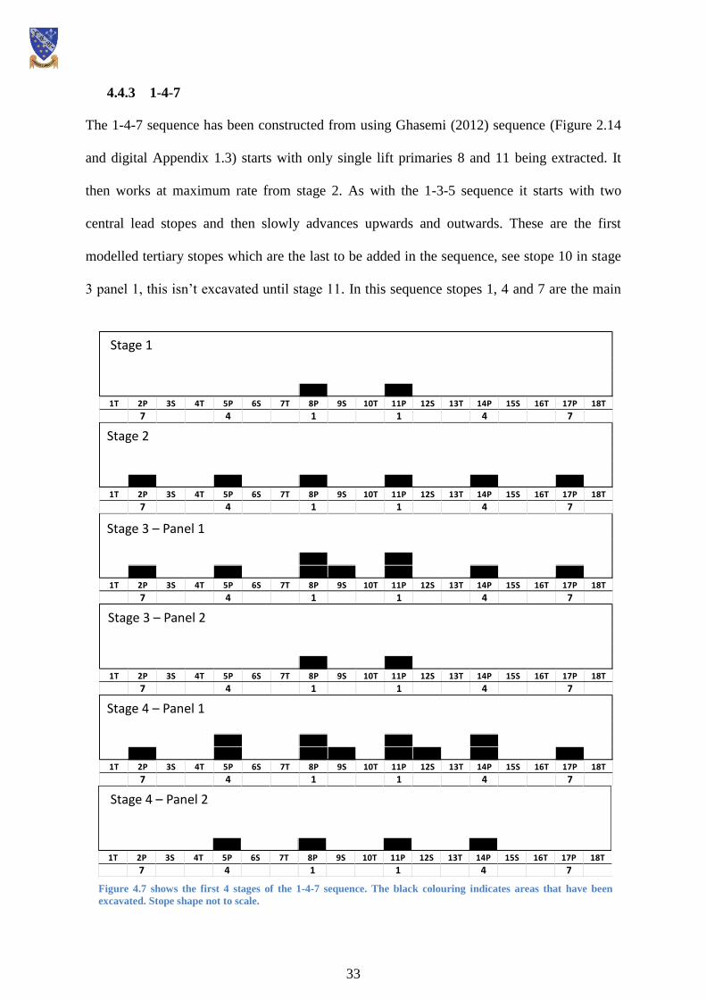
4.4.3 1-4-7
The 1-4-7 sequence has been constructed from using Ghasemi (2012) sequence (Figure 2.14
and digital Appendix 1.3) starts with only single lift primaries 8 and 11 being extracted. It
then works at maximum rate from stage 2. As with the 1-3-5 sequence it starts with two
central lead stopes and then slowly advances upwards and outwards. These are the first
modelled tertiary stopes which are the last to be added in the sequence, see stope 10 in stage
3 panel 1, this isn’t excavated until stage 11. In this sequence stopes 1, 4 and 7 are the main
0 0 0 0 0 0 0 0 0 0 0 0 0 0 0 0 0 0
0 0 0 0 0 0 0 0 0 0 0 0 0 0 0 0 0 0
0 0 0 0 0 0 0 0 0 0 0 0 0 0 0 0 0 0
0 0 0 0 0 0 0 0 0 0 0 0 0 0 0 0 0 0
0 0 0 0 0 0 0 1 0 0 1 0 0 0 0 0 0 0
1T 2P 3S 4T 5P 6S 7T 8P 9S 10T 11P 12S 13T 14P 15S 16T 17P 18T
7 4 1 1 4 7
0 0 0 0 0 0 0 0 0 0 0 0 0 0 0 0 0 0
0 0 0 0 0 0 0 0 0 0 0 0 0 0 0 0 0 0
0 0 0 0 0 0 0 0 0 0 0 0 0 0 0 0 0 0
0 0 0 0 0 0 0 0 0 0 0 0 0 0 0 0 0 0
0 1 0 0 1 0 0 1 0 0 1 0 0 1 0 0 1 0
1T 2P 3S 4T 5P 6S 7T 8P 9S 10T 11P 12S 13T 14P 15S 16T 17P 18T
7 4 1 1 4 7
0 0 0 0 0 0 0 0 0 0 0 0 0 0 0 0 0 0
0 0 0 0 0 0 0 0 0 0 0 0 0 0 0 0 0 0
0 0 0 0 0 0 0 0 0 0 0 0 0 0 0 0 0 0
0 0 0 0 0 0 0 1 0 0 1 0 0 0 0 0 0 0
0 1 0 0 1 0 0 1 1 0 1 0 0 1 0 0 1 0
1T 2P 3S 4T 5P 6S 7T 8P 9S 10T 11P 12S 13T 14P 15S 16T 17P 18T
7 4 1 1 4 7
0 0 0 0 0 0 0 0 0 0 0 0 0 0 0 0 0 0
0 0 0 0 0 0 0 0 0 0 0 0 0 0 0 0 0 0
0 0 0 0 0 0 0 0 0 0 0 0 0 0 0 0 0 0
0 0 0 0 0 0 0 0 0 0 0 0 0 0 0 0 0 0
0 0 0 0 0 0 0 1 0 0 1 0 0 0 0 0 0 0
1T 2P 3S 4T 5P 6S 7T 8P 9S 10T 11P 12S 13T 14P 15S 16T 17P 18T
7 4 1 1 4 7
0 0 0 0 0 0 0 0 0 0 0 0 0 0 0 0 0 0
0 0 0 0 0 0 0 0 0 0 0 0 0 0 0 0 0 0
0 0 0 0 0 0 0 0 0 0 0 0 0 0 0 0 0 0
0 0 0 0 1 0 0 1 0 0 1 0 0 1 0 0 0 0
0 1 0 0 1 0 0 1 1 0 1 1 0 1 0 0 1 0
1T 2P 3S 4T 5P 6S 7T 8P 9S 10T 11P 12S 13T 14P 15S 16T 17P 18T
7 4 1 1 4 7
0 0 0 0 0 0 0 0 0 0 0 0 0 0 0 0 0 0
0 0 0 0 0 0 0 0 0 0 0 0 0 0 0 0 0 0
0 0 0 0 0 0 0 0 0 0 0 0 0 0 0 0 0 0
0 0 0 0 0 0 0 0 0 0 0 0 0 0 0 0 0 0
0 0 0 0 1 0 0 1 0 0 1 0 0 1 0 0 0 0
1T 2P 3S 4T 5P 6S 7T 8P 9S 10T 11P 12S 13T 14P 15S 16T 17P 18T
7 4 1 1 4 7
Stage 1
Stage 2
Stage 3 – Panel 1
Stage 3 – Panel 2
Stage 4 – Panel 1
Stage 4 – Panel 2
Figure 4.7 shows the first 4 stages of the 1-4-7 sequence. The black colouring indicates areas that have been
excavated. Stope shape not to scale.

34
lead stopes with 4 being a stope or two behind 1 and 7 a similar delay behind 4. The lead
stope experience high stresses as a result of the high level of confinement but create a ‘bow
wave’ effect that tends to de-stress adjacent primary stopes.
The other 3 sequences have been designed to be 19 stopes wide. The 1-4-7 sequence is only
18 stopes wide because the single mining front presented itself more effectively in 18 stopes
as opposed to 19 stopes. However this will have minimal impact upon the stress results
overall.
4.4.4 1-5-9
Stopes 1-5-9 are extracted as two lift primaries and filled with consolidated fill (Figure 2.15
and digital Appendix 1.4). This is followed by another set of primary two lift stopes (3-7-11),
0 0 0 0 0 0 0 0 0 0 0 0 0 0 0 0 0 0 0
0 0 0 0 0 0 0 0 0 0 0 0 0 0 0 0 0 0 0
0 0 0 0 0 0 0 0 0 0 0 0 0 0 0 0 0 0 0
0 0 0 0 0 0 0 0 0 0 0 0 0 0 0 0 0 0 0
0 0 0 0 0 0 0 0 0 1 0 0 0 0 0 0 0 0 0
1S 2P 3T 4S 5T 6P 7T 8S 9T 10P 11T 12S 13T 14P 15T 16S 17T 18P 19S
9 5 1 5 90 0 0 0 0 0 0 0 0 0 0 0 0 0 0 0 0 0 0
0 0 0 0 0 0 0 0 0 0 0 0 0 0 0 0 0 0 0
0 0 0 0 0 0 0 0 0 0 0 0 0 0 0 0 0 0 0
0 0 0 0 0 0 0 0 0 0 0 0 0 0 0 0 0 0 0
0 0 0 0 0 1 0 0 0 1 0 0 0 1 0 0 0 0 0
1S 2P 3T 4S 5T 6P 7T 8S 9T 10P 11T 12S 13T 14P 15T 16S 17T 18P 19S
9 5 1 5 9
0 0 0 0 0 0 0 0 0 0 0 0 0 0 0 0 0 0 0
0 0 0 0 0 0 0 0 0 0 0 0 0 0 0 0 0 0 0
0 0 0 0 0 0 0 0 0 0 0 0 0 0 0 0 0 0 0
0 0 0 0 0 0 0 0 0 1 0 0 0 0 0 0 0 0 0
0 0 0 0 0 1 0 1 0 1 0 1 0 1 0 0 0 0 0
1S 2P 3T 4S 5T 6P 7T 8S 9T 10P 11T 12S 13T 14P 15T 16S 17T 18P 19S
9 5 1 5 90 0 0 0 0 0 0 0 0 0 0 0 0 0 0 0 0 0 0
0 0 0 0 0 0 0 0 0 0 0 0 0 0 0 0 0 0 0
0 0 0 0 0 0 0 0 0 0 0 0 0 0 0 0 0 0 0
0 0 0 0 0 0 0 0 0 1 0 0 0 0 0 0 0 0 0
0 1 0 0 0 1 0 1 0 1 0 1 0 1 0 0 0 1 0
1S 2P 3T 4S 5T 6P 7T 8S 9T 10P 11T 12S 13T 14P 15T 16S 17T 18P 19S
9 5 1 5 9
0 0 0 0 0 0 0 0 0 0 0 0 0 0 0 0 0 0 0
0 0 0 0 0 0 0 0 0 0 0 0 0 0 0 0 0 0 0
0 0 0 0 0 0 0 0 0 0 0 0 0 0 0 0 0 0 0
0 0 0 0 0 0 0 0 0 0 0 0 0 0 0 0 0 0 0
0 0 0 0 0 0 0 0 0 1 0 0 0 0 0 0 0 0 0
1S 2P 3T 4S 5T 6P 7T 8S 9T 10P 11T 12S 13T 14P 15T 16ST 17T 18P 19S
9 5 1 5 9
Stage 1
Stage 2
Stage 3
Stage 4 – Panel 2
Stage 4 – Panel 1
Figure 4.8 shows the first 4 stages of the 1-5-9 sequence. The black colouring indicates areas that have
been excavated. Stope shape not to scale.

35
also filled with consolidated fill. Following the fill cure within the primary stopes 1-3-5-7-9-
11, a set of single lift stopes (2-6-10) is then extracted and filled with unconsolidated fill.
This creates a pendant pillar, which has many degrees of freedom and relies on the fill
support from the primary stopes for stability. Finally, the single lift stopes 4-8-12 are
extracted and filled with unconsolidated fill before the entire sequence is repeated up-dip.
The extraction of stopes 4-8-12 also creates pendant pillars (Ghasemi, 2012).

36
5. Investigating Damage
The analysis of the models must be carried out with a method of quantifying areas of high
stress into damage or yield. With a contoured output, as shown in Figure 5.1 general
indications of stress and its location can easily be made however when trying to quantify the
exact value at an exact point is impossible with the eye.
The analysis section therefore will make use of query lines and points for the analysis of the
model outputs, see the three query lines Figure 5.1. They are set to a particular coordinate in
x, y and z space and will provide the exact value at each point. Figure 5.1 is a σ3 stress
representation of a single stope and the query lines indicate the σ3 stress on the excavation
boundary. This data can then be plotted in graph form to show the relative stress across an
excavation for example.
This thesis’ aim is to investigate stress and damage induced by different sequences. In any
rock mass being able to predict under what stress or strain conditions yield or damage will
occur is extremely difficult. There are many contributing factors that in one condition will
damage the rock but in others will not. Board et al. (2001) suggests criteria under which rock
can be classified depending on the induced stress interaction of σ1 and σ3:
Solids: Sigma 3 Total
-1.4
0.9
3.1
5.4
7.7
9.9
12.2
14.4
16.6
18.9
21.1
min (all): -1.16447 MPa
min (stage): -1.16447 MPa
max (stage): 20.3547 MPa
max (all): 20.3547 MPa
σ3- Unfilled
Figure 5.1 is an example of the use of query lines to extract exact data from a contour result
37
Minimal Damage: General slabbing along drifts but not very deep. Affecting 20% to 30% of
tunnel width or height, standard support is adequate with only minor rehab required. This
damage corresponds to a ratio of:
(σ1 - σ3)/unconfined compressive strength (UCS) of approx. 0.2 (20%) or less.
This will be characterised by a DS differential of 30MPa or less.
Moderate Damage: Heavier slabbing along drifts with wall broke into blocks affecting 30%-
50% of tunnel width or height. Will generally require some rehab, particularly at intersections
or wide spans. Rehab may consist of scaling, additional bolts, and a thin layer of shotcrete.
This damage corresponds to a ratio of
(σ1 - σ3) /UCS of approximately 0.2 – 0.4 (20% - 40%).
This will be characterised by a DS differential of 30MPa – 60MPa.
High Damage Potential: Here, the value of the major principal stress nears the uniaxial
compressive strength of the rock mass. In Rhyolites, this results in significant deterioration,
large closures and potential groundfall hazard. In massive sulphides or andesites this
condition means a high potential for seismicity. The host rock at OD is breccia so doesn’t fit
these criteria however this level of damage corresponds to a ratio of:
(σ1 – σ3) /UCS of approximately 0.4 or higher
This will be characterised by a DS differential 60MPa or higher.
This classification system is known as DS (DS) and uses figures of σ1 and σ3 to classify the
level of damage. RS3 can model this output into a contoured result which will show
concentrated areas of high or low DS. With the use of query lines the actual DS can be
determined and be ranked according to this classification system. DS is unitless in RS3

38
however it is a difference of two MPa values and therefore will be given MPa as units.
Martin et al. (1999) argues however in a similar vein that σ3 on its own is critical. Martin et
al. finds that when σ3 exceeds -0.8MPa, tensile failure will occur. In these analyses the depth
of the σ3 = 0 isosurface for the HW at the mid height of the stope was recorded rather than
the rock mass tensile strength. This approach seems more appropriate because once the
confinement is reduced to zero the rock mass is free to dilate and unravel under gravity
loading.
Therefore both criteria agree but Martin et al.’s conclusion puts less significance on a high σ1
that is implied in Board (2001)’s classification. For the interpretation of the results of this
thesis, the classification set out by Board (2001) will be used. However regions of
particularly low confining stress will be investigated to determine stability and damage.
To identify the areas of low DS query points will be used to target specific positions within
the stope block according to where the greatest DS concentration is. This could be argued as
a biased sampling strategy by not considering the rest of the stope, however in mining and
stope extraction it is the small areas with highest readings that are critical. These must be
identified, examined and steps be taken to minimise their impact on safety and production
within the operation.
An unbiased set of query points will be used to produce an average across all of the stages of
the sequence. These will be positioned at a central point within the each stope that can then
be averaged and compared for a general overview of maximum, minimum and average DS
conditions for a comparison.
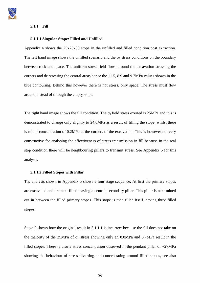
39
5.1.1 Fill
5.1.1.1 Singular Stope: Filled and Unfilled
Appendix 4 shows the 25x25x30 stope in the unfilled and filled condition post extraction.
The left hand image shows the unfilled scenario and the σ1 stress conditions on the boundary
between rock and space. The uniform stress field flows around the excavation stressing the
corners and de-stressing the central areas hence the 11.5, 8.9 and 9.7MPa values shown in the
blue contouring. Behind this however there is not stress, only space. The stress must flow
around instead of through the empty stope.
The right hand image shows the fill condition. The σ1 field stress exerted is 25MPa and this is
demonstrated to change only slightly to 24.6MPa as a result of filling the stope, whilst there
is minor concentration of 0.2MPa at the corners of the excavation. This is however not very
constructive for analysing the effectiveness of stress transmission in fill because in the real
stop condition there will be neighbouring pillars to transmit stress. See Appendix 5 for this
analysis.
5.1.1.2 Filled Stopes with Pillar
The analysis shown in Appendix 5 shows a four stage sequence. At first the primary stopes
are excavated and are next filled leaving a central, secondary pillar. This pillar is next mined
out in between the filled primary stopes. This stope is then filled itself leaving three filled
stopes.
Stage 2 shows how the original result in 5.1.1.1 is incorrect because the fill does not take on
the majority of the 25MPa of σ1 stress showing only an 8.8MPa and 8.7MPa result in the
filled stopes. There is also a stress concentration observed in the pendant pillar of ~27MPa
showing the behaviour of stress diverting and concentrating around filled stopes, see also
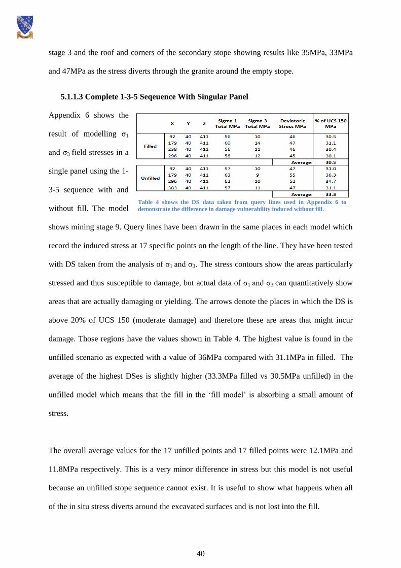
40
stage 3 and the roof and corners of the secondary stope showing results like 35MPa, 33MPa
and 47MPa as the stress diverts through the granite around the empty stope.
5.1.1.3 Complete 1-3-5 Seqeuence With Singular Panel
Appendix 6 shows the
result of modelling σ1
and σ3 field stresses in a
single panel using the 1-
3-5 sequence with and
without fill. The model
shows mining stage 9. Query lines have been drawn in the same places in each model which
record the induced stress at 17 specific points on the length of the line. They have been tested
with DS taken from the analysis of σ1 and σ3. The stress contours show the areas particularly
stressed and thus susceptible to damage, but actual data of σ1 and σ3 can quantitatively show
areas that are actually damaging or yielding. The arrows denote the places in which the DS is
above 20% of UCS 150 (moderate damage) and therefore these are areas that might incur
damage. Those regions have the values shown in Table 4. The highest value is found in the
unfilled scenario as expected with a value of 36MPa compared with 31.1MPa in filled. The
average of the highest DSes is slightly higher (33.3MPa filled vs 30.5MPa unfilled) in the
unfilled model which means that the fill in the ‘fill model’ is absorbing a small amount of
stress.
The overall average values for the 17 unfilled points and 17 filled points were 12.1MPa and
11.8MPa respectively. This is a very minor difference in stress but this model is not useful
because an unfilled stope sequence cannot exist. It is useful to show what happens when all
of the in situ stress diverts around the excavated surfaces and is not lost into the fill.
Table 4 shows the DS data taken from query lines used in Appendix 6 to
demonstrate the difference in damage vulnerability induced without fill.

41
5.1.2 Olympic Dam Stress conditions
In Figure 5.2 a single excavated stope is tested along with a second panel of one stope to
assess how the stress will act on an elongated structure in the –Z direction. Figure 5.2 shows
how the principal stress hits the excavation at 135° and concentrates the stress in the corners
normal to this stress, with values of 57.8MPa and 48.3MPa in stage 1. It is particularly high
at this stage because it is a single excavated region, therefore the stress can only flow through
the stope walls and not through the excavation. With the addition of fill in stage 2 a little
stress dissipates through the fill lowering the corner stress to 50.7MPa and 42.8MPa. Stage 3
sees the excavation of the second panel in the –Z direction. Upon excavation the maximum
stress is lower still (48.2MPa and 43.2MPa) because this time the induced stress is acting
over 50m of excavation rather than 25m and this lessening its concentration. The fill in the
first stope has also now begun to deform applying pressure on the fill and improving its
ability to transmit stress. In the centre of the first stope the σ1 stress is as much as 14MPa in
stage 3. When the second stope is then filled the fill hasn’t had the chance to be compressed
fully and therefore produces values of 0.0. The two main corner stresses are 45.3MPa (not
0.0MPa as shown by the vertex query) and 43.2MPa.
Solids: Sigma 1 Total
0.0
6.0
12.0
18.0
24.0
30.0
36.0
42.0
48.0
54.0
60.0
min (all): 0 MPa
min (stage): 14.3119 MPa
max (stage): 57.9989 MPa
max (all): 58.2444 MPa
Solids: Sigma 1 Total
0.0
6.0
12.0
18.0
24.0
30.0
36.0
42.0
48.0
54.0
60.0
min (all): 0 MPa
min (stage): 7.62674 MPa
max (stage): 50.855 MPa
max (all): 58.2444 MPa
Solids: Sigma 1 Total
0.0
6.0
12.0
18.0
24.0
30.0
36.0
42.0
48.0
54.0
60.0
min (all): 0 MPa
min (stage): 7.65122 MPa
max (stage): 58.2444 MPa
max (all): 58.2444 MPa
Solids: Sigma 1 Total
0.0
6.0
12.0
18.0
24.0
30.0
36.0
42.0
48.0
54.0
60.0
min (all): 0 MPa
min (stage): 0 MPa
max (stage): 53.9121 MPa
max (all): 58.2444 MPa
Stage 1 Stage 3
Stage 2 Stage 4
σ1 σ
1
σ1 σ
1
Figure 5.2 show how the Olympic Dam stress conditions present themselves upon a single stope under σ1 stress contours

42
6. Results and Analysis
This section will take the reader through the results found from the modelling of the four
separate sequences. The rock conditions have been discussed in the methodology but they
will refer to shifts in the stress regime.
The main objective of each sequence is to manage the principal virgin stresses so that as they
deform around the excavated area they concentrate in the abutments at the excavation
periphery. In this way the damage to the rock is sustained away from the areas being mined.
RS3 contains a suite of data type analysis modes. In each case query lines have been used to
extract data from the models from which calculations, graphs and quantitative comparisons
can be made to differentiate the positives and negatives of each sequence. Throughout this
section the three primary-secondary (tertiary) sequences will be compared with the
continuous sequence and each other.
Using the three groups of damage criteria; minimal, moderate and high, the models are
investigated for vulnerable regions as products of the sequence. Using DS (σ1 – σ3) as an
analogue for regions of rock at risk of failure, a stress contour can be queried to provide a
value for DS. The damage criteria have been defined in section 5 and will be used to assess
damage in the sequences.
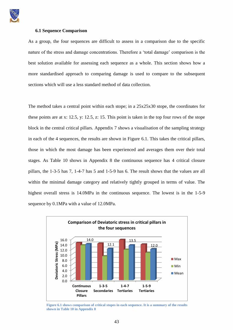
43
6.1 Sequence Comparison
As a group, the four sequences are difficult to assess in a comparison due to the specific
nature of the stress and damage concentrations. Therefore a ‘total damage’ comparison is the
best solution available for assessing each sequence as a whole. This section shows how a
more standardised approach to comparing damage is used to compare to the subsequent
sections which will use a less standard method of data collection.
The method takes a central point within each stope; in a 25x25x30 stope, the coordinates for
these points are at x: 12.5, y: 12.5, z: 15. This point is taken in the top four rows of the stope
block in the central critical pillars. Appendix 7 shows a visualisation of the sampling strategy
in each of the 4 sequences, the results are shown in Figure 6.1. This takes the critical pillars,
those in which the most damage has been experienced and averages them over their total
stages. As Table 10 shows in Appendix 8 the continuous sequence has 4 critical closure
pillars, the 1-3-5 has 7, 1-4-7 has 5 and 1-5-9 has 6. The result shows that the values are all
within the minimal damage category and relatively tightly grouped in terms of value. The
highest overall stress is 14.0MPa in the continuous sequence. The lowest is in the 1-5-9
sequence by 0.1MPa with a value of 12.0MPa.
0.0
2.0
4.0
6.0
8.0
10.0
12.0
14.0
16.0
ContinuousClosurePillars
1-3-5Secondaries
1-4-7Tertiaries
1-5-9Tertiaries
14.0 12.1
13.5
12.0
De
viat
ori
c St
ress
(M
Pa)
Comparison of Deviatoric stress in critical pillars in the four sequences
Max
Min
Mean
Figure 6.1 shows comparison of critical stopes in each sequence. It is a summary of the results
shown in Table 10 in Appendix 8
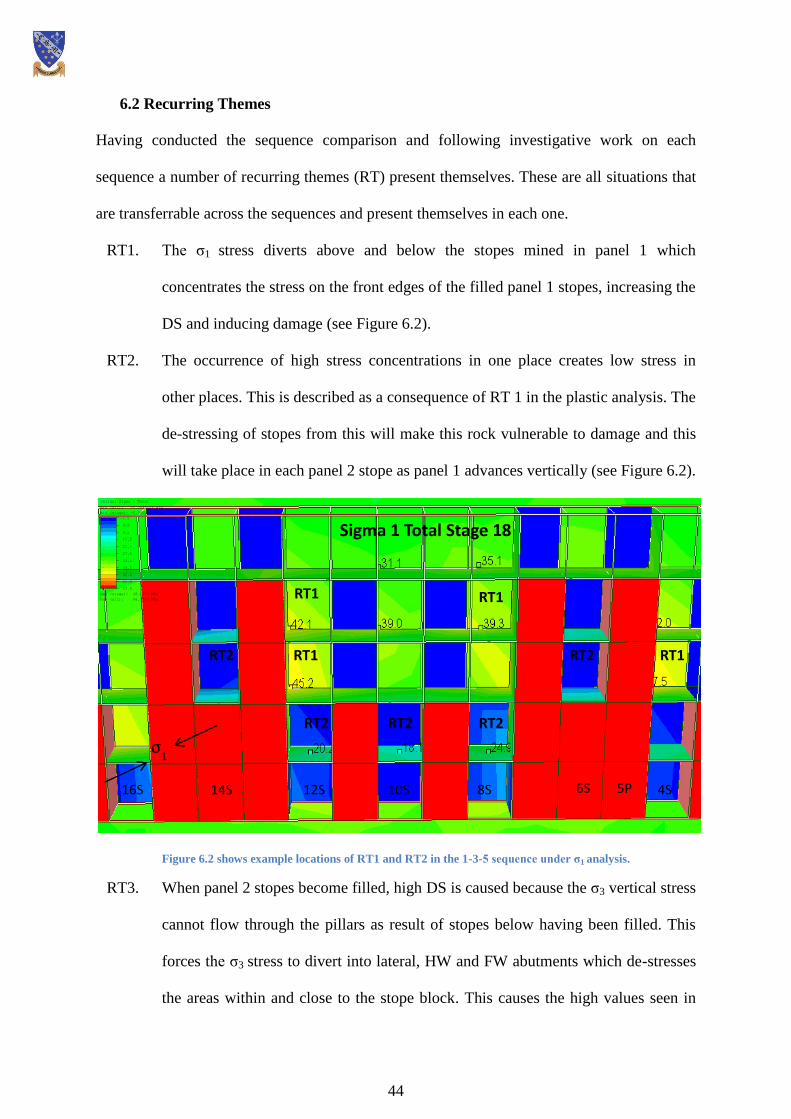
44
6.2 Recurring Themes
Having conducted the sequence comparison and following investigative work on each
sequence a number of recurring themes (RT) present themselves. These are all situations that
are transferrable across the sequences and present themselves in each one.
RT1. The σ1 stress diverts above and below the stopes mined in panel 1 which
concentrates the stress on the front edges of the filled panel 1 stopes, increasing the
DS and inducing damage (see Figure 6.2).
RT2. The occurrence of high stress concentrations in one place creates low stress in
other places. This is described as a consequence of RT 1 in the plastic analysis. The
de-stressing of stopes from this will make this rock vulnerable to damage and this
will take place in each panel 2 stope as panel 1 advances vertically (see Figure 6.2).
Figure 6.2 shows example locations of RT1 and RT2 in the 1-3-5 sequence under σ1 analysis.
RT3. When panel 2 stopes become filled, high DS is caused because the σ3 vertical stress
cannot flow through the pillars as result of stopes below having been filled. This
forces the σ3 stress to divert into lateral, HW and FW abutments which de-stresses
the areas within and close to the stope block. This causes the high values seen in
Solids: Sigma 1 Total
-2.5
3.5
9.5
15.5
21.5
27.5
33.5
39.5
45.5
51.5
57.5
min (all): -0.0695506 MPa
min (stage): -0.0456369 MPa
max (stage): 48.1778 MPa
max (all): 66.9808 MPa
RT1
RT2 RT2 RT2
RT2 RT2
RT1 RT1
RT1
Sigma 1 Total Stage 18
σ1
14S 12S 10S 8S 6S 5P 4S 16S
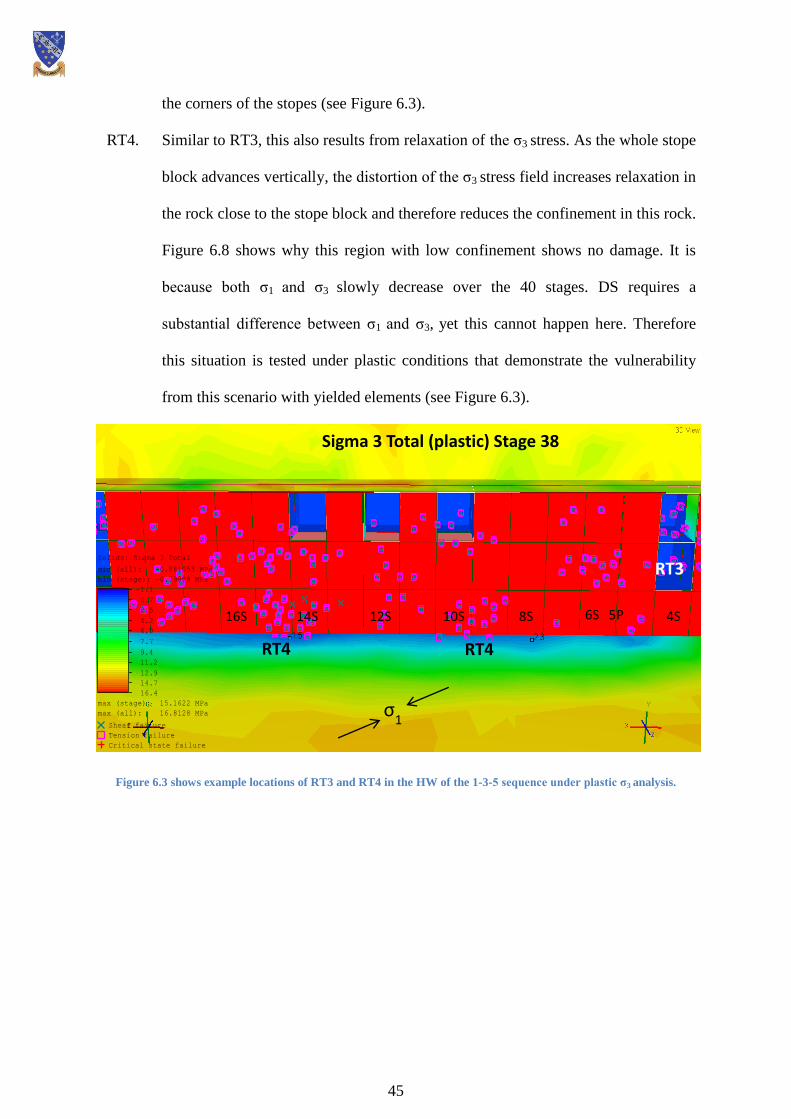
45
the corners of the stopes (see Figure 6.3).
RT4. Similar to RT3, this also results from relaxation of the σ3 stress. As the whole stope
block advances vertically, the distortion of the σ3 stress field increases relaxation in
the rock close to the stope block and therefore reduces the confinement in this rock.
Figure 6.8 shows why this region with low confinement shows no damage. It is
because both σ1 and σ3 slowly decrease over the 40 stages. DS requires a
substantial difference between σ1 and σ3, yet this cannot happen here. Therefore
this situation is tested under plastic conditions that demonstrate the vulnerability
from this scenario with yielded elements (see Figure 6.3).
Figure 6.3 shows example locations of RT3 and RT4 in the HW of the 1-3-5 sequence under plastic σ3 analysis.
Solids: Sigma 3 Total
-1.1
0.7
2.5
4.2
6.0
7.7
9.4
11.2
12.9
14.7
16.4
min (all): -0.881053 MPa
min (stage): -0.79828 MPa
max (stage): 15.1622 MPa
max (all): 16.8128 MPa
Shear failure
Tension failure
Critical state failure
σ1
Sigma 3 Total (plastic) Stage 38
RT4 RT4
RT3
14S 12S 10S 8S 6S 5P 4S 16S
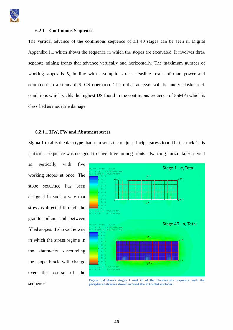
46
6.2.1 Continuous Sequence
The vertical advance of the continuous sequence of all 40 stages can be seen in Digital
Appendix 1.1 which shows the sequence in which the stopes are excavated. It involves three
separate mining fronts that advance vertically and horizontally. The maximum number of
working stopes is 5, in line with assumptions of a feasible roster of man power and
equipment in a standard SLOS operation. The initial analysis will be under elastic rock
conditions which yields the highest DS found in the continuous sequence of 55MPa which is
classified as moderate damage.
6.2.1.1 HW, FW and Abutment stress
Sigma 1 total is the data type that represents the major principal stress found in the rock. This
particular sequence was designed to have three mining fronts advancing horizontally as well
as vertically with five
working stopes at once. The
stope sequence has been
designed in such a way that
stress is directed through the
granite pillars and between
filled stopes. It shows the way
in which the stress regime in
the abutments surrounding
the stope block will change
over the course of the
sequence.
Stage 1 - σ1
Total
Solids: Sigma 1 Total
-1.5
6.0
13.5
21.0
28.5
36.0
43.5
51.0
58.5
66.0
73.5
min (all): -0.0820228 MPa
min (stage): -0.0233779 MPa
max (stage): 50.5623 MPa
max (all): 67.0402 MPa
Solids: Sigma 1 Total
23.9
24.2
24.5
24.8
25.2
25.5
25.8
26.1
26.5
26.8
27.1
min (all): -0.0820228 MPa
min (stage): 23.8594 MPa
max (stage): 27.0268 MPa
max (all): 67.0402 MPa
Stage 40 - σ1
Total
Figure 6.4 shows stages 1 and 40 of the Continuous Sequence with the
peripheral stresses shown around the extruded surfaces.
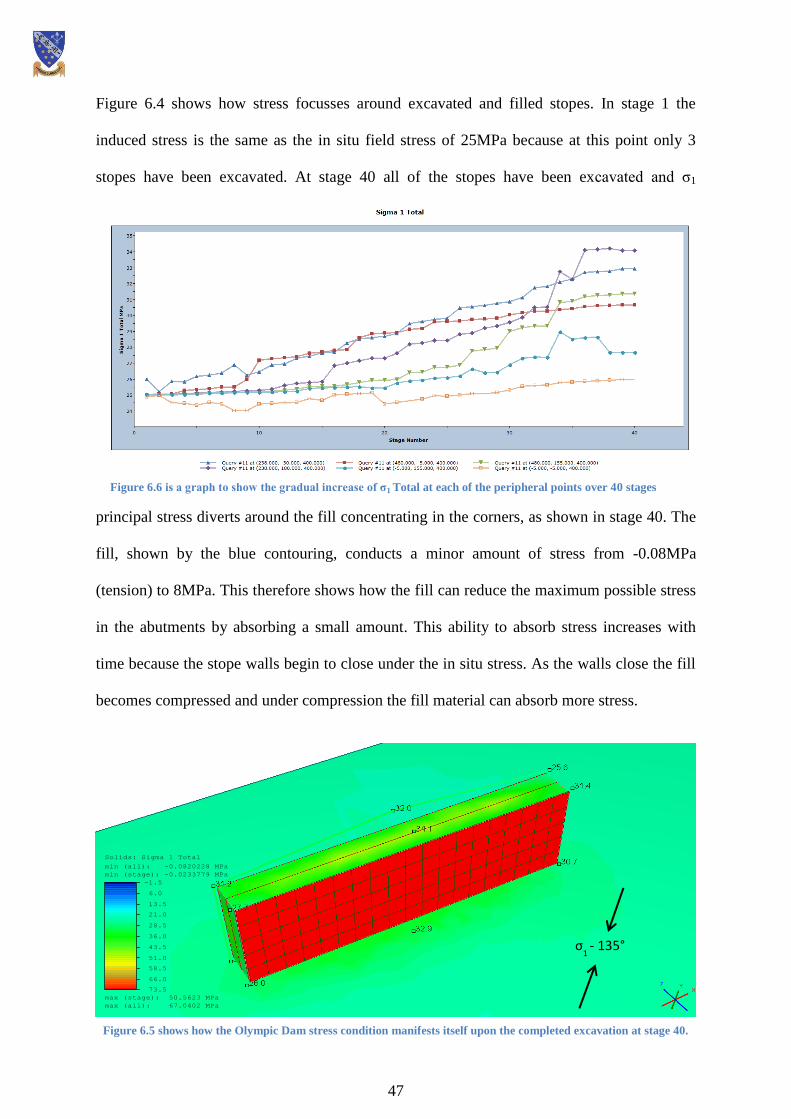
47
Figure 6.6 is a graph to show the gradual increase of σ1 Total at each of the peripheral points over 40 stages
Figure 6.4 shows how stress focusses around excavated and filled stopes. In stage 1 the
induced stress is the same as the in situ field stress of 25MPa because at this point only 3
stopes have been excavated. At stage 40 all of the stopes have been excavated and σ1
principal stress diverts around the fill concentrating in the corners, as shown in stage 40. The
fill, shown by the blue contouring, conducts a minor amount of stress from -0.08MPa
(tension) to 8MPa. This therefore shows how the fill can reduce the maximum possible stress
in the abutments by absorbing a small amount. This ability to absorb stress increases with
time because the stope walls begin to close under the in situ stress. As the walls close the fill
becomes compressed and under compression the fill material can absorb more stress.
σ1
- 135°
Solids: Sigma 1 Total
-1.5
6.0
13.5
21.0
28.5
36.0
43.5
51.0
58.5
66.0
73.5
min (all): -0.0820228 MPa
min (stage): -0.0233779 MPa
max (stage): 50.5623 MPa
max (all): 67.0402 MPa
Figure 6.5 shows how the Olympic Dam stress condition manifests itself upon the completed excavation at stage 40.
48
Figure 6.6 shows how the σ1 stress becomes increasingly concentrated in the abutments as the
excavation extent increases over the stages. The highest stress in Figure 6.6 is found in the
top left corner value of 27.7MPa which is lower than the value shown in the top right corner
of 31.4MPa. This is due to the orientation of σ1 at 135°. This concept was explored in section
5.1.2 with the Olympic Dam stress concentrating around an angular structure.
6.2.1.2 Intra Stope Damage
The analysis in Figure 6.7 shows stage 22 and 24 which has been constructed using an x-y
plane and an x-z plane at the base of row 3. There are also surface contours along the top of
rows 3, 4 and 5 to show the distribution of damage through the stopes and pillars. The green
and yellow areas indicate higher DS and therefore damage. Query lines and points have been
used to illustrate the DS at different locations at different stages. These regions have been
investigated because high DS concentrations indicate failings in the sequence.
The four stages observed in Figure 6.7 and 6.9 are not the only stages in which high values
have been found, however to investigate all of them would be repetitive to analyse. The
original DS at all of the points is 12.5MPa, the difference between the virgin principal
stresses.
Stage 22 in Figure 6.7 shows five points A, B, C, D and E. Regions A and D show a
deviation of 30.2MPa and 29.4MPa and the maximum for the whole stage is 34.4MPa
(moderate damage). These points are located within two pendant pillars or stress windows
that focus the σ1 stress and lessen the σ3 principal stress.

49
Figure 6.7 shows the relative influence of each principal stress. The σ1 stress concentration is
a function of the composition of the rock versus the fill and the shape of the stopes. The stope
shape, combined with the strategically located competent rock, provide an easier path than
the fill material which is taken by the stress. The σ1 stress has to divert above and below the
stopes mined in panel 1 which concentrates the stress on the front edges of the filled stopes
increasing the DS and inducing damage (RT1)
There is a high deviation here because the σ3 vertical stress cannot flow through the pillars as
result of stopes below having been filled. This forces the σ3 stress to divert into lateral, HW
and FW abutments which de-stresses the areas within and close to the stope block (RT3).
Figure 6.7 shows five points A, B, C, D and E at stages 22 and 24 in the continuous sequence under DS
analysis. The whole excavation cannot be seen due to a YZ plane intersecting the stopes to the right of the
Figure.
Solids: Deviatoric Stress
0.0
5.0
10.0
15.0
20.0
25.0
30.0
35.0
40.0
45.0
50.0
min (all): 0.000147126
min (stage): 0.00491248
max (stage): 34.3735
max (all): 55.6818
Solids: Deviatoric Stress
0.0
5.0
10.0
15.0
20.0
25.0
30.0
35.0
40.0
45.0
50.0
min (all): 0.000147126
min (stage): 0.00364088
max (stage): 45.6556
max (all): 55.6818
DS - Stage 22
DS - Stage 24
σ1
A
B
C
D
E
σ1
Max: 45.6 MPa
Max: 34.3 MPa
A
B
C
D
E
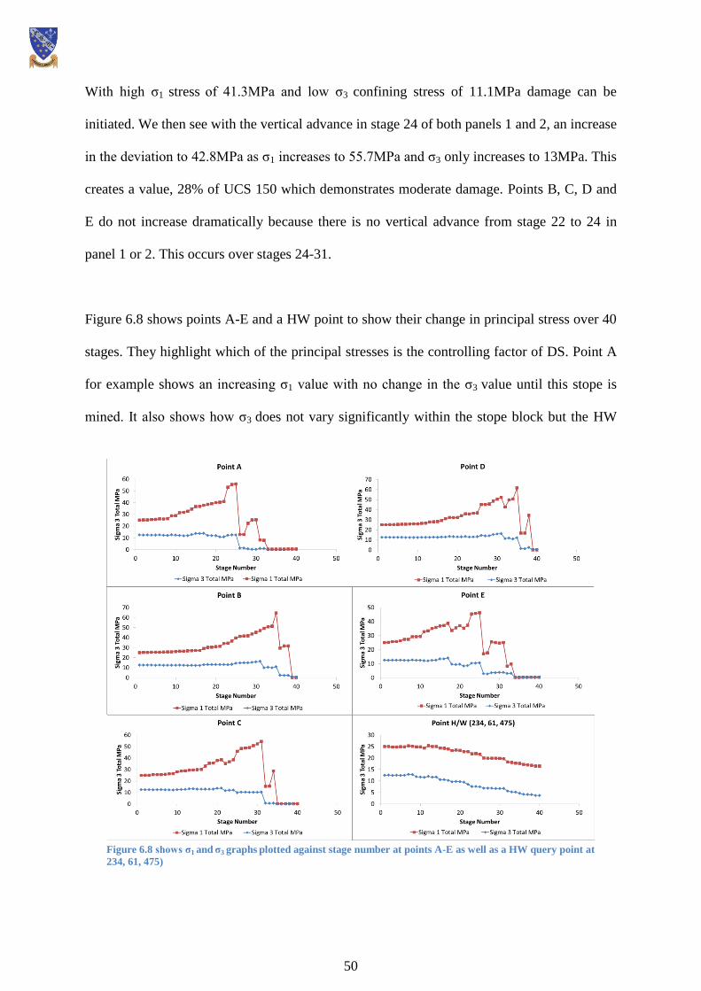
50
With high σ1 stress of 41.3MPa and low σ3 confining stress of 11.1MPa damage can be
initiated. We then see with the vertical advance in stage 24 of both panels 1 and 2, an increase
in the deviation to 42.8MPa as σ1 increases to 55.7MPa and σ3 only increases to 13MPa. This
creates a value, 28% of UCS 150 which demonstrates moderate damage. Points B, C, D and
E do not increase dramatically because there is no vertical advance from stage 22 to 24 in
panel 1 or 2. This occurs over stages 24-31.
Figure 6.8 shows points A-E and a HW point to show their change in principal stress over 40
stages. They highlight which of the principal stresses is the controlling factor of DS. Point A
for example shows an increasing σ1 value with no change in the σ3 value until this stope is
mined. It also shows how σ3 does not vary significantly within the stope block but the HW
Figure 6.8 shows σ1 and σ3 graphs plotted against stage number at points A-E as well as a HW query point at
234, 61, 475)

51
point shows that outside of the stope block, σ3 is more susceptible to change. The HW point,
25m away from the back of panel 2, shows that both σ1 and σ3 slowly decrease over the 40
stages. It is this region in the plastic analysis that suffers high yield and this graph provides
evidence of why this occurs (RT4).
Move through the sequence 7 stages to stage 31, the region around A has been mined in stage
30 and is about to be filled. It cannot therefore carry any induced stress and shows a value of
0.4MPa. Points B, C and E however have increased their values to 46.5MPa, 30.9MPa and
38.6MPa respectively, increasing moderate damage. This is a reaction to the increase in
height of the pillar where they are situated. Before the B and C pillar was only 30m high and
the σ1 value was only 38MPa. The pillar height increases to 60m and that value increases to
56.3MPa which is almost in the high damage potential bracket. The stress focusses in the left
corner due to the orientation of the σ1 stress. It comes around the corner of the fill of panel 1
Solids: Deviatoric Stress
0.0
5.0
10.0
15.0
20.0
25.0
30.0
35.0
40.0
45.0
50.0
min (all): 0.000147126
min (stage): 0.00968501
max (stage): 47.0938
max (all): 55.6818
DS - Stage 35
DS - Stage 31
Solids: Deviatoric Stress
0.0
5.6
11.2
16.8
22.4
28.0
33.6
39.2
44.8
50.4
56.0
min (all): 0.000147126
min (stage): 0.00867519
max (stage): 55.4822
max (all): 55.4822
σ1
σ1
Max: 55.4 MPa
Max: 47.1 MPa
A B
C
D
E
A B
C
D
E
Figure 6.9 shows five points A, B, C, D and E at stages 31 and 35 in the continuous sequence under DS
analysis.

52
and 2 and concentrates along the boundary between panel 1 and 2 and in the far wall. The
contouring around point B shows how the damage extends out into the pillar which will cause
complications later on in the sequence for the drilling and development teams. The damage
however does not extend out into the HW behind panel 2 as is shown by the horizontal
contour plane at 58m.
Stage 35 sees a further concentration of σ1 stress at points C and E with point B under
relaxation from the filling of the stope below. The DS is reduced to 0.8MPa which, as with
the low HW σ3 stress creates issues due to low confinement. Figure 6.9 shows this pre-mining
dip in σ1 and σ3 at point B in stage 35. The plastic analysis will highlight this weakness.
6.2.1.3 Plastic Analysis
Up to this stage in the analysis all of the models have been run as elastic and therefore do not
present any yielded structures or a post-peak rock condition. Following the analysis of critical
regions, an analysis based upon a plastic rock reaction must be performed. The rock will not
perform perfectly plastic at all times however this analysis highlights areas which are most
vulnerable whilst also being able to compare yield between sequences. Plastic rock reaction
will show a reduced peak stress due to the failed plastic rock’s inability to transmit stress
Solids: Sigma 1 Total
10.0
14.8
19.6
24.4
29.2
34.0
38.8
43.6
48.4
53.2
58.0
min (all): -0.406938 MPa
min (stage): -0.019008 MPa
max (stage): 50.3575 MPa
max (all): 58.2272 MPa
Shear failure
Tension failure
Critical state failure
σ1
σ1 Total/Yielded elements- Stage 40
Figure 6.10 shows stage 40 under Plastic, σ1 total analysis with yielded elements.
FW
HW
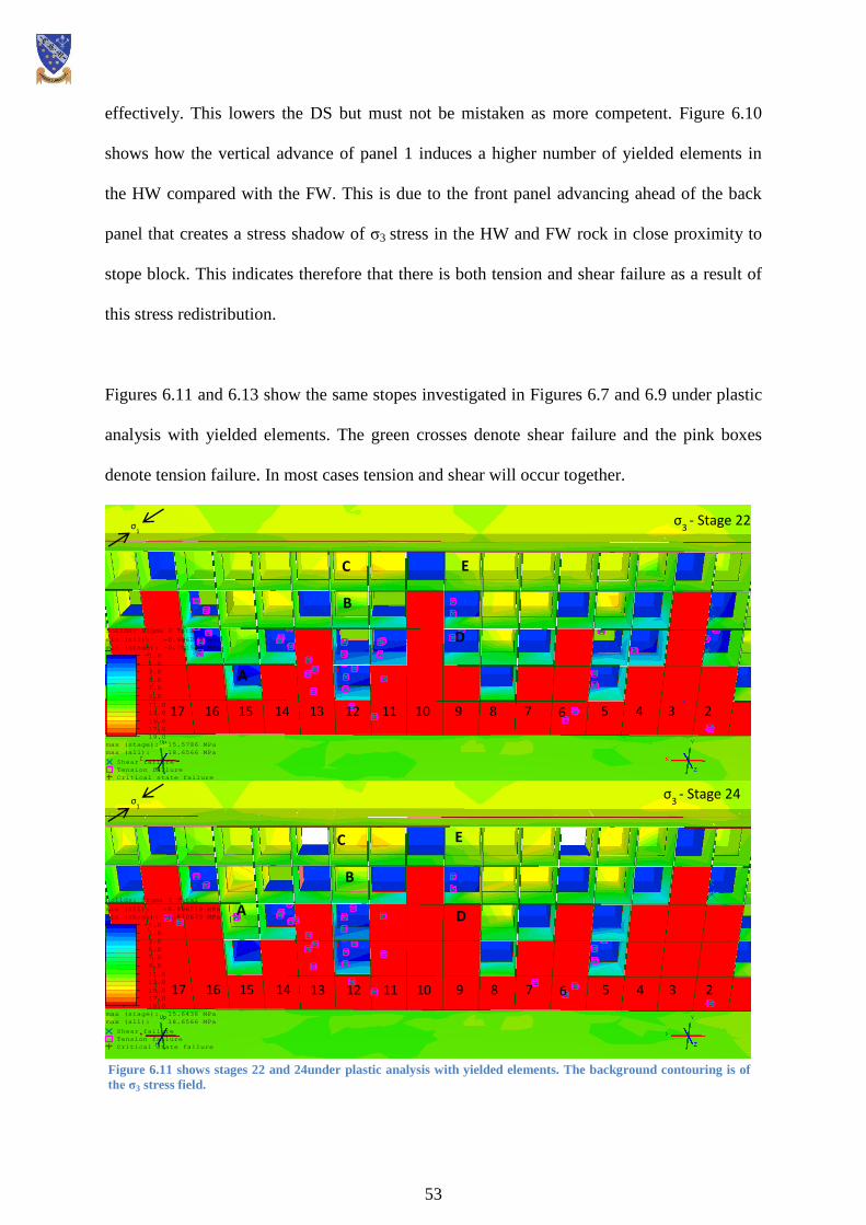
53
effectively. This lowers the DS but must not be mistaken as more competent. Figure 6.10
shows how the vertical advance of panel 1 induces a higher number of yielded elements in
the HW compared with the FW. This is due to the front panel advancing ahead of the back
panel that creates a stress shadow of σ3 stress in the HW and FW rock in close proximity to
stope block. This indicates therefore that there is both tension and shear failure as a result of
this stress redistribution.
Figures 6.11 and 6.13 show the same stopes investigated in Figures 6.7 and 6.9 under plastic
analysis with yielded elements. The green crosses denote shear failure and the pink boxes
denote tension failure. In most cases tension and shear will occur together.
Figure 6.11 shows stages 22 and 24under plastic analysis with yielded elements. The background contouring is of
the σ3 stress field.
Solids: Sigma 3 Total
-1.0
1.0
3.0
5.0
7.0
9.0
11.0
13.0
15.0
17.0
19.0
min (all): -0.906219 MPa
min (stage): -0.670673 MPa
max (stage): 15.6436 MPa
max (all): 18.6566 MPa
Shear failure
Tension failure
Critical state failure
Solids: Sigma 3 Total
-1.0
1.0
3.0
5.0
7.0
9.0
11.0
13.0
15.0
17.0
19.0
min (all): -0.906219 MPa
min (stage): -0.701589 MPa
max (stage): 15.5786 MPa
max (all): 18.6566 MPa
Shear failure
Tension failure
Critical state failure
σ3
- Stage 22
σ3
- Stage 24
17 16 15 14 13 12 11 10 9 8 7 6 5 4 3 2
17 16 15 14 13 12 11 10 9 8 7 6 5 4 3 2
σ1
σ1
A
B
C
D
E
A
B
C
D
E
54
Stage 22 in the elastic analysis showed moderate damage with a DS value of 34MPa. The
area around point A, which showed the highest DS in the elastic analysis, must be noted as
showing no yield under plastic conditions. The yielded elements seen in line with stopes 13,
11 and 6 are all located in the HW and the regions where yielded elements are located in line
with 5, 9, 12 and 16 are within the stope block in pendant pillars. The pendant pillar yields
are located where there is a vertical advance in panel 1 which de-stresses them, reducing the
confining stress and putting them at risk of failure. Even if the DS in elastic analysis deems
there to be damage it is the low σ3 stress that also induces damage. In this model, once an
element has yielded its symbol stays in the result to show that this feature has yielded so
therefore the image is a cumulative representation of all of the yielded elements to that point.
Stage 24 shows a similar result to stage 22. Point A has the highest DS and yet is not the area
with the most yield. Row 2 and 3 in pendant pillar 12 presents significant yield. Using a
query point, the software reveals that this area at a height of 40m has a value for σ1 of
5.8MPa, σ2 of 0.12MPa and a σ3 of -0.005MPa (tension). It is this induced stress regime that
instigates the yielding presented here and is potentially hazardous if this area becomes
damaged in the lead up to the mining. With confining stress, the damaged rock remains
stable, but once the stress is released by mining or if there a change in adjacent stope
conditions confinement is released and damage propagates.
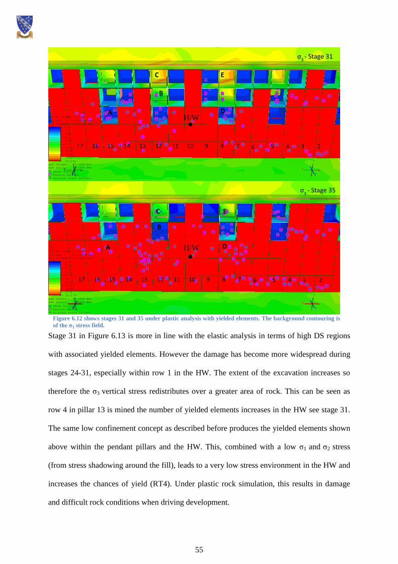
55
Stage 31 in Figure 6.13 is more in line with the elastic analysis in terms of high DS regions
with associated yielded elements. However the damage has become more widespread during
stages 24-31, especially within row 1 in the HW. The extent of the excavation increases so
therefore the σ3 vertical stress redistributes over a greater area of rock. This can be seen as
row 4 in pillar 13 is mined the number of yielded elements increases in the HW see stage 31.
The same low confinement concept as described before produces the yielded elements shown
above within the pendant pillars and the HW. This, combined with a low σ1 and σ2 stress
(from stress shadowing around the fill), leads to a very low stress environment in the HW and
increases the chances of yield (RT4). Under plastic rock simulation, this results in damage
and difficult rock conditions when driving development.
Solids: Sigma 3 Total
-1.0
1.0
3.0
5.0
7.0
9.0
11.0
13.0
15.0
17.0
19.0
min (all): -0.906219 MPa
min (stage): -0.894135 MPa
max (stage): 17.4288 MPa
max (all): 18.6566 MPa
Shear failure
Tension failure
Critical state failure
Solids: Sigma 3 Total
-1.0
1.0
3.0
5.0
7.0
9.0
11.0
13.0
15.0
17.0
19.0
min (all): -0.906219 MPa
min (stage): -0.899222 MPa
max (stage): 16.4848 MPa
max (all): 18.6566 MPa
Shear failure
Tension failure
Critical state failure
σ3
- Stage 35
σ3
- Stage 31
17 16 15 14 13 12 11 10 9 8 7 6 5 4 3 2
17 16 15 14 13 12 11 10 9 8 7 6 5 4 3 2
Figure 6.12 shows stages 31 and 35 under plastic analysis with yielded elements. The background contouring is
of the σ3 stress field.
A
B
C
D
E
A
B
C
D
E
H/W
H/W

56
Stage 35 shows RT2. Pillars 5, 8, and 15 in row 4, all show yielded elements within the stope
itself. This is due to the low σ3 created from the σ1 stress diverting above and below the panel
1 stopes discussed
previously. While the σ1
stress concentrates
around the filled panel 1
stopes, the rock in panel
2 stope becomes
unconfined from the low
σ3 stress hence the blue
colouration in figure 6.13. The DS shows up no damage in elastic analysis because the σ1 is
also low but the low confinement makes this rock vulnerable and this is shown in the plastic
analysis.
A noticeable omission from the yielded elements result is yield in the crown and below the
mined area. As shown in stage 40 in Figure 6.10 there is almost no yield in the area above the
fill. This is also the case for the area beneath. One possible explanation is that in this region
confining stresses are not being shadowed and the confining stress remains high and therefore
no yield occurs unless this area was later de-stressed by future development.
6.2.2 Sequence 1-3-5
Unlike the continuous sequence there are primary stopes in the 1-3-5 sequence which are
extracted and filled before the secondary stopes. This allows stress to be diverted or
channelled by future secondary stopes which act as pillars to convey the stress. As the
secondary stopes are mined, they no longer fulfil the role of pillars and the design of the
Figure 6.13 shows data from a query point in the H/W with the graphs for σ1, σ2
and σ3 over the 40 stages of the continuous sequence.
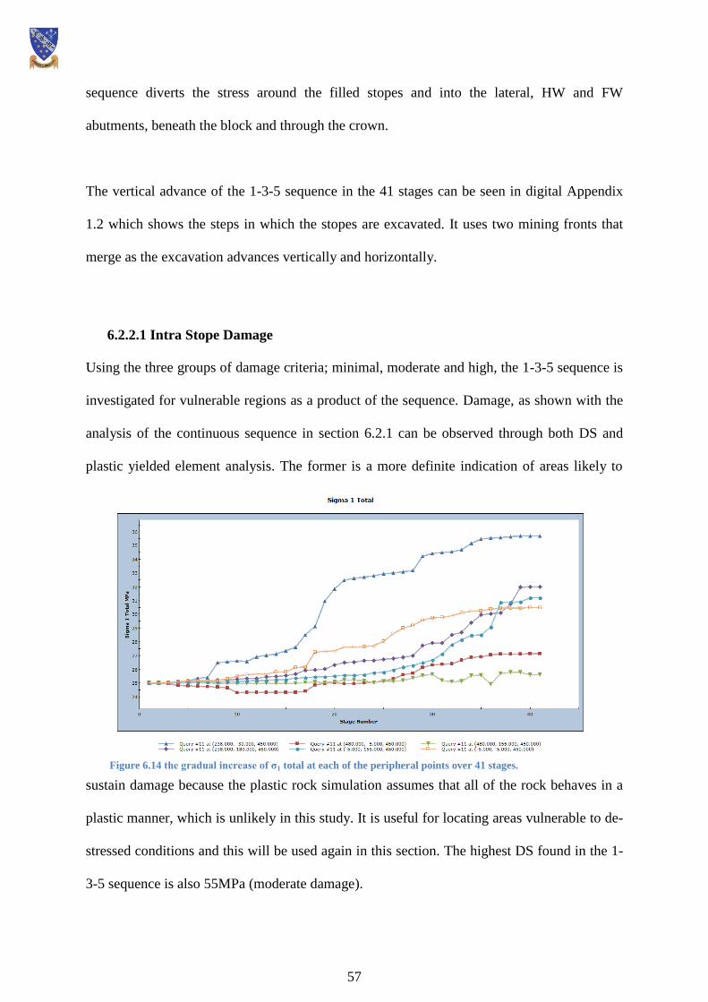
57
sequence diverts the stress around the filled stopes and into the lateral, HW and FW
abutments, beneath the block and through the crown.
The vertical advance of the 1-3-5 sequence in the 41 stages can be seen in digital Appendix
1.2 which shows the steps in which the stopes are excavated. It uses two mining fronts that
merge as the excavation advances vertically and horizontally.
6.2.2.1 Intra Stope Damage
Using the three groups of damage criteria; minimal, moderate and high, the 1-3-5 sequence is
investigated for vulnerable regions as a product of the sequence. Damage, as shown with the
analysis of the continuous sequence in section 6.2.1 can be observed through both DS and
plastic yielded element analysis. The former is a more definite indication of areas likely to
sustain damage because the plastic rock simulation assumes that all of the rock behaves in a
plastic manner, which is unlikely in this study. It is useful for locating areas vulnerable to de-
stressed conditions and this will be used again in this section. The highest DS found in the 1-
3-5 sequence is also 55MPa (moderate damage).
Figure 6.14 the gradual increase of σ1 total at each of the peripheral points over 41 stages.
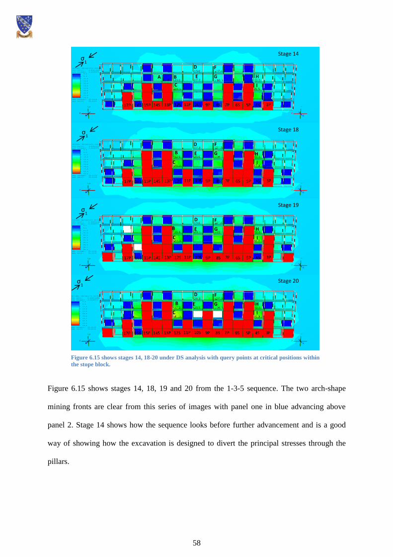
58
Figure 6.15 shows stages 14, 18, 19 and 20 from the 1-3-5 sequence. The two arch-shape
mining fronts are clear from this series of images with panel one in blue advancing above
panel 2. Stage 14 shows how the sequence looks before further advancement and is a good
way of showing how the excavation is designed to divert the principal stresses through the
pillars.
Solids: Deviatoric Stress
0.0
5.6
11.2
16.8
22.4
28.0
33.6
39.2
44.8
50.4
56.0
min (all): 0.000102962
min (stage): 0.0246471
max (stage): 55.2139
max (all): 55.2139
Solids: Deviatoric Stress
0.0
5.6
11.2
16.8
22.4
28.0
33.6
39.2
44.8
50.4
56.0
min (all): 0.000102962
min (stage): 0.0246471
max (stage): 55.2139
max (all): 55.2139
Solids: Deviatoric Stress
0.0
5.6
11.2
16.8
22.4
28.0
33.6
39.2
44.8
50.4
56.0
min (all): 0.000102962
min (stage): 0.0246471
max (stage): 55.2139
max (all): 55.2139
Solids: Deviatoric Stress
0.0
5.6
11.2
16.8
22.4
28.0
33.6
39.2
44.8
50.4
56.0
min (all): 0.000102962
min (stage): 0.0246471
max (stage): 55.2139
max (all): 55.2139
Stage 14
Stage 18
Stage 19
Stage 20 σ1
σ1
σ1
σ1
A B C
D
E F G H
I
B
C
D
E
F G H
I
B
C
D
E F G H
I
B
C
D
E
F
G H I
3P 4S 5P 6S 7P 8S 9P 10S 11P 12S 13P 14S 15P 16S 17P
3P 4S 5P 6S 7P 8S 9P 10S 11P 12S 13P 14S 15P 16S 17P
3P 4S 5P 6S 7P 8S 9P 10S 11P 12S 13P 14S 15P 16S 17P
3P 4S 5P 6S 7P 8S 9P 10S 11P 12S 13P 14S 15P 16S 17P
Figure 6.15 shows stages 14, 18-20 under DS analysis with query points at critical positions within
the stope block.
59
Points B, C, G and I show how the principal stresses concentrate in the pillars. These points
show particularly high values compared with the others because of the primary stopes
influence on the flow of the in situ stress. The σ1 stress flows at 135° around the primaries
and focusses in the opposite walls. The σ3 stress acts vertically, but because of its 225° trend
the primary stopes in panel 1 create a stress shadowed area in the right hand wall of the filled
stopes. Therefore the σ1 stress is concentrated in this wall where the σ3 stress is low. (RT1).
As with the continuous sequence there is a lack of confinement (RT2) and therefore the
possibility of damage. Therefore points C and I, each with a DS of 29.5MPa or moderate
damage, will be subjected to higher stress environments in later stages as the overall
excavated region grows.
Stage 18 is the first of three stages in the closure of the central three pillars. These are
particularly high stress environments and logic would suggest that as a result these would
sustain the most damage compared with other stages in the sequence. Figure 6.15 shows that
the maximum DS at this stage is ~37.9MPa (moderate damage) at point I which is not located
in the central pillars. Stress concentrates here because point I is in pillar 4S of the right-hand
mining front (RT1). The main principal stress concentrates around this corner first and the
location at the foot of the tallest pillar of filled stopes creates a stress shadow within this area
as σ3 is diverted by the highest filled stopes (RT3).
Figure 6.16 shows how pillar 10S presents a low stress contour at point 2 that is has a σ1
value of 18.1MPa, σ3 of 9.4MPa and σ2 of 13.6MPa (RT1). This is de-stressed in comparison
to points C, B and G whose σ1 values are double of those seen at 1, 2 and 3. When this area is
tested with yielded elements it is likely to present high levels of yield. However under elastic
conditions stage 18 can be considered low risk with DS of 18MPa showing minimal damage.

60
Stage 19 is the closure
of pillars 8S and 12S.
The impact on the DS is
minor, changing point
B from 36MPa to
37MPa which shows
that the vertical, σ3
stress is not altered greatly upon pillar closure. Stage 20 is then the closure of the central
pillar 10S which creates further de-stressing of the stopes above (RT2). The σ1 value drops
from 19MPa to 11.8MPa with the backfilling of the central stope. Two central stopes are
being mined simultaneous to the filling which put a 49.7MPa of σ1 stress through the only
available gap in the excavation at 90m in height. The result is a DS of 41MPa which is the
highest value up to this point in the sequence and moderately damaged.
Figure 6.17 shows stages 32 and 34 focussing on the centre seven stopes, the area that has
consistently shown high potential for damage thus far in the 1-3-5 sequence. It aims to
highlight the difference in damage conditions across the stope depth by using query lines in
the central stopes x, y and z. For example, in stage 32 the range from the back to the front of
stopes x, y and z is 11MPa, 15MPa and 15MPa respectively. This kind of stress imbalance in
homogeneous, competent and brittle granite will create damage across the width of the stope
which will create issues when it comes to mining. These queries highlight the level to which
these central stopes become de-stressed. With the σ1 stress having to divert up and over the
filled stopes in panel 1 (RT1) it leaves stope x and y in the stress shadow of the front panel
(RT2). The query lines also show that lower rows of stopes are more de-stressed that the
higher ones as a result of the σ1 stress deflection. The front point in stope x is 11MPa
4S 5P 6S 7P 8S 9P 10S 11P 12S 13P 14S 15P 16S
Solids: Sigma 1 Total
-2.5
3.5
9.5
15.5
21.5
27.5
33.5
39.5
45.5
51.5
57.5
min (all): -0.0695506 MPa
min (stage): -0.0456369 MPa
max (stage): 48.1778 MPa
max (all): 66.9808 MPa
B
C
D
E
F
G H
I
3 2 1
Figure 6.16 shows stage 18 under σ1 analysis. It shows the relative de-stressing of the
three pillars at points 1, 2 and 3 in comparison to the points B, C, E and G above.
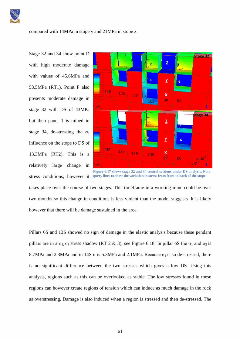
61
compared with 14MPa in stope y and 21MPa in stope z.
Stage 32 and 34 show point D
with high moderate damage
with values of 45.6MPa and
53.5MPa (RT1). Point F also
presents moderate damage in
stage 32 with DS of 43MPa
but then panel 1 is mined in
stage 34, de-stressing the σ1
influence on the stope to DS of
13.3MPa (RT2). This is a
relatively large change in
stress conditions; however it
takes place over the course of two stages. This timeframe in a working mine could be over
two months so this change in conditions is less violent than the model suggests. It is likely
however that there will be damage sustained in the area.
Pillars 6S and 13S showed no sign of damage in the elastic analysis because these pendant
pillars are in a σ1, σ3 stress shadow (RT 2 & 3), see Figure 6.18. In pillar 6S the σ1 and σ3 is
8.7MPa and 2.3MPa and in 14S it is 5.3MPa and 2.1MPa. Because σ1 is so de-stressed, there
is no significant difference between the two stresses which gives a low DS. Using this
analysis, regions such as this can be overlooked as stable. The low stresses found in these
regions can however create regions of tension which can induce as much damage in the rock
as overstressing. Damage is also induced when a region is stressed and then de-stressed. The
Figure 6.17 shows stage 32 and 34 central sections under DS analysis. Note
query lines to show the variation in stress from front to back of the stope.
Solids: Deviatoric Stress
0.0
5.6
11.2
16.8
22.4
28.0
33.6
39.2
44.8
50.4
56.0
min (all): 0.000102962
min (stage): 0.0246471
max (stage): 55.2139
max (all): 55.2139
Solids: Deviatoric Stress
0.0
5.6
11.2
16.8
22.4
28.0
33.6
39.2
44.8
50.4
56.0
min (all): 0.000102962
min (stage): 0.00725663
max (stage): 49.9524
max (all): 55.2139
D
E
F
G
D
E
F
G
Stage 32
Stage 34
X
8S 9P 10S 11P
12S 13P
X
8S 9P 10S
11P 12S 13P
Y
Z
Y
Z
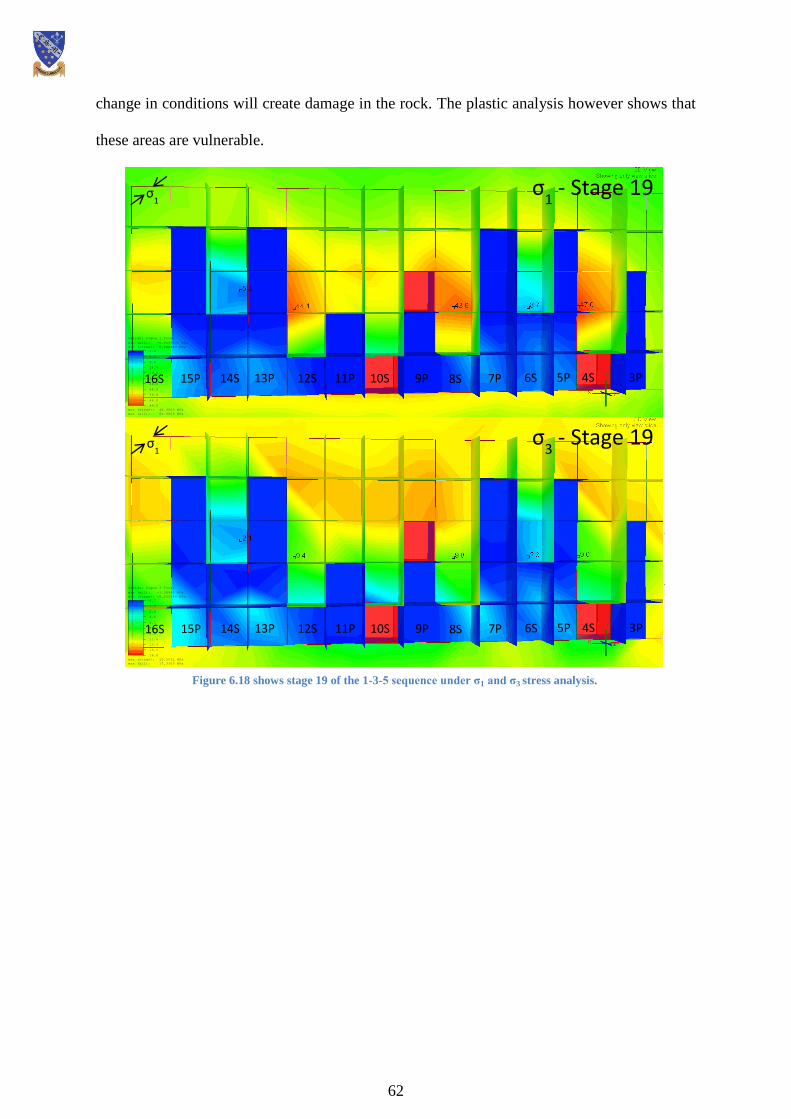
62
change in conditions will create damage in the rock. The plastic analysis however shows that
these areas are vulnerable.
Solids: Sigma 1 Total
-1.0
4.0
9.0
14.0
19.0
24.0
29.0
34.0
39.0
44.0
49.0
min (all): -0.0695506 MPa
min (stage): -0.048946 MPa
max (stage): 48.3063 MPa
max (all): 66.9808 MPa
Solids: Sigma 3 Total
-0.7
1.0
2.8
4.5
6.3
8.1
9.8
11.6
13.3
15.1
16.8
min (all): -1.38943 MPa
min (stage): -0.632646 MPa
max (stage): 15.5032 MPa
max (all): 17.3359 MPa
σ1 σ
3 - Stage 19
σ1 - Stage 19 σ
1
3P 4S 5P 6S 7P 8S 9P 10S 11P 12S 13P 14S 15P 16S
3P 4S 5P 6S 7P 8S 9P 10S 11P 12S 13P 14S 15P 16S
Figure 6.18 shows stage 19 of the 1-3-5 sequence under σ1 and σ3 stress analysis.

63
6.2.2.2 Plastic Analysis
The plastic result for the 1-3-5 sequence is very different when compared with the continuous
sequence. Figure 6.19 demonstrates how the yielded elements are much less numerous at this
stage showing only slight yield in the secondary pillars. As the elastic analysis has shown at
stage 18, this is a critical stage for the central three secondary pillars (S11, S10 and S8). Each
of these pillars are 60m in height and at their most susceptible in terms of their hydraulic
radius. They do not however show significant yield. There is an area of low stress in S10 that
comes about as a result of RT4, shown in Figure 6.19.
Primary pillar P13 shows the first signs of plastic damage out into the HW with four yielded
elements from 35m in height to 90m (RT4). The furthest that the yield extends at this stage is
18m into the HW. As was suggested in the analysis of Figure 6.18, row three stopes in pillar
S14 and S6 shows yielded elements in the stress shadowed region. This will have
repercussions later in the sequence upon mining of these stopes.
Figure 6.19 shows stage 18 of the 1-5-9 sequence under plastic analysis
Solids: Deviatoric Stress
0.0
4.5
9.0
13.5
18.0
22.5
27.0
31.5
36.0
40.5
45.0
min (all): 0.000103498
min (stage): 0.00201763
max (stage): 38.476
max (all): 43.854
Shear failure
Tension failure
Critical state failure
Stage 18
T16 S14 S12 S10 S8 S6 S4
σ1
P13

64
Stage 32 and 38 are shown under plastic analysis and σ3 stress in Figure 6.20. It shows how
the yielded elements in the HW are induced as a result of low σ3 stress in close proximity to
the face panel 2. Two query points at 61m show the σ3 values amongst the cluster of yielded
elements of 2.3MPa and 3.1MPa in stage 32. As the excavation advances upwards the yielded
elements increase and these σ3 values drop to 1.5MPa and 2.3MPa in stage 30. Therefore this
yield is brought about by the low confining stress brought about by the height of the stoping
block (RT4).
Solids: Sigma 3 Total
-1.1
0.7
2.5
4.2
6.0
7.7
9.4
11.2
12.9
14.7
16.4
min (all): -0.881053 MPa
min (stage): -0.85553 MPa
max (stage): 15.9922 MPa
max (all): 16.8128 MPa
Shear failure
Tension failure
Critical state failure
Solids: Sigma 3 Total
-1.1
0.7
2.5
4.2
6.0
7.7
9.4
11.2
12.9
14.7
16.4
min (all): -0.881053 MPa
min (stage): -0.79828 MPa
max (stage): 15.1622 MPa
max (all): 16.8128 MPa
Shear failure
Tension failure
Critical state failure
σ1
σ1
σ3 - Stage 38
σ3 - Stage 32
S13 S11 S10 S8 S6 S6
S13 S11 S10 S8 S6 S6 S4
S4
Figure 6.20 shows stage 32 and 38 under plastic analysis and σ3 stress contouring
65
The Recurring Themes discussed at length in sections 6.2.1 and 6.2.2 are also investigated in
the 1-4-7 and 1-5-9 sequence. The bulk of these analyses are found in Appendix 9 and 10.
This has been done to ensure that the main body of the does not repeat the same analysis just
for a separate sequence. Here follows a brief summary of both those sequences.
6.2.3 Sequence 1-4-7
The 1-4-7 sequence is similar to the 1-3-5 sequence with primary and secondary pillars but
has the addition of tertiary stopes. All 39 stages can be seen in digital Appendix 1.3. As was
shown in section 4.4.3 two central primary pillars advance upwards together in position 1
with pillars 4 and 7 following one and two stopes behind. The secondary pillars advance 2
stopes behind the primaries on one side of the primaries leaving the tertiary pillars ideally 2
stopes behind the secondaries. The highest DS found in the 1-4-7 sequence is 52.9MPa which
is classified as moderate damage.
6.2.4 Sequence 1-5-9
The 1-5-9 sequence is based upon a singular mining front advancing vertically and
horizontally as used in the 1-4-7 sequence. The 1-4-7 only ran 18 stopes widths but the 1-5-9
sequence is 19 stopes (375m) across. The sequence can be seen in the methodology section
4.4.4 taken from Ghasemi (2011). The initial stages are run not in line with this sequence
however to maximise active stopes without doing continuous stoping. The vertical advance of
the 1-5-9 sequence in all 43 stages can be seen in digital Appendix 1.4. The highest DS found
in the 1-5-9 sequence is 49MPa which is the lowest of the four sequences and is classified as
moderate damage.
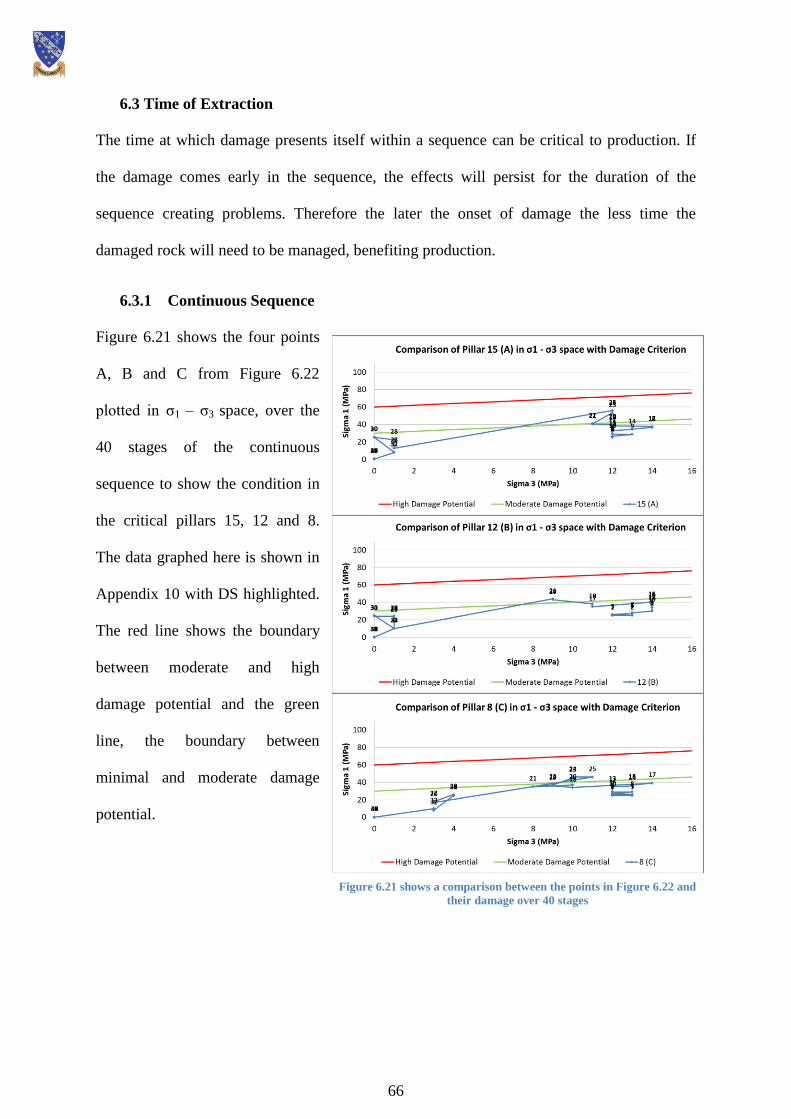
66
6.3 Time of Extraction
The time at which damage presents itself within a sequence can be critical to production. If
the damage comes early in the sequence, the effects will persist for the duration of the
sequence creating problems. Therefore the later the onset of damage the less time the
damaged rock will need to be managed, benefiting production.
6.3.1 Continuous Sequence
Figure 6.21 shows the four points
A, B and C from Figure 6.22
plotted in σ1 – σ3 space, over the
40 stages of the continuous
sequence to show the condition in
the critical pillars 15, 12 and 8.
The data graphed here is shown in
Appendix 10 with DS highlighted.
The red line shows the boundary
between moderate and high
damage potential and the green
line, the boundary between
minimal and moderate damage
potential.
Figure 6.21 shows a comparison between the points in Figure 6.22 and
their damage over 40 stages
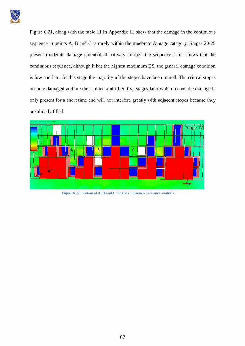
67
Figure 6.21, along with the table 11 in Appendix 11 show that the damage in the continuous
sequence in points A, B and C is rarely within the moderate damage category. Stages 20-25
present moderate damage potential at halfway through the sequence. This shows that the
continuous sequence, although it has the highest maximum DS, the general damage condition
is low and late. At this stage the majority of the stopes have been mined. The critical stopes
become damaged and are then mined and filled five stages later which means the damage is
only present for a short time and will not interfere greatly with adjacent stopes because they
are already filled.
Stage 17
A C B
Solids: Deviatoric Stress
0.0
5.0
10.0
15.0
20.0
25.0
30.0
35.0
40.0
45.0
50.0
min (all): 0
min (stage): 0.00102299
max (stage): 38.7133
max (all): 49.5085
Figure 6.22 location of A, B and C for the continuous sequence analysis
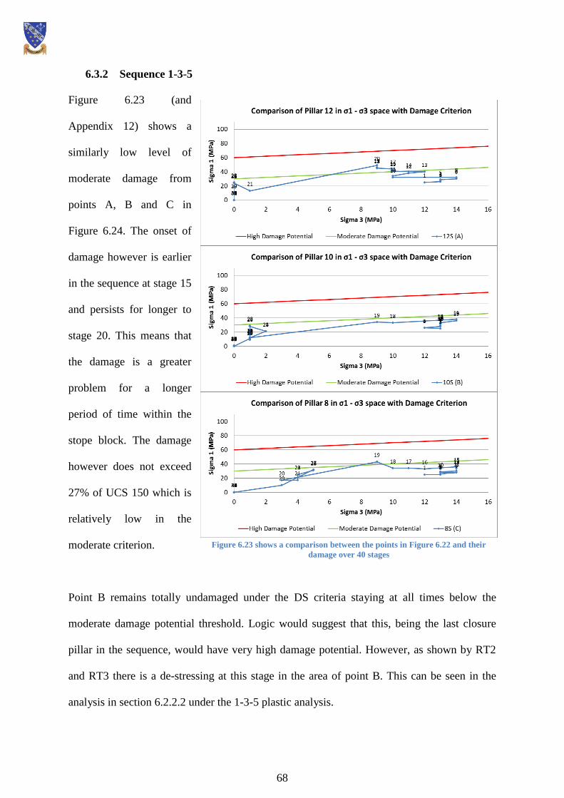
68
6.3.2 Sequence 1-3-5
Figure 6.23 (and
Appendix 12) shows a
similarly low level of
moderate damage from
points A, B and C in
Figure 6.24. The onset of
damage however is earlier
in the sequence at stage 15
and persists for longer to
stage 20. This means that
the damage is a greater
problem for a longer
period of time within the
stope block. The damage
however does not exceed
27% of UCS 150 which is
relatively low in the
moderate criterion.
Point B remains totally undamaged under the DS criteria staying at all times below the
moderate damage potential threshold. Logic would suggest that this, being the last closure
pillar in the sequence, would have very high damage potential. However, as shown by RT2
and RT3 there is a de-stressing at this stage in the area of point B. This can be seen in the
analysis in section 6.2.2.2 under the 1-3-5 plastic analysis.
Figure 6.23 shows a comparison between the points in Figure 6.22 and their
damage over 40 stages
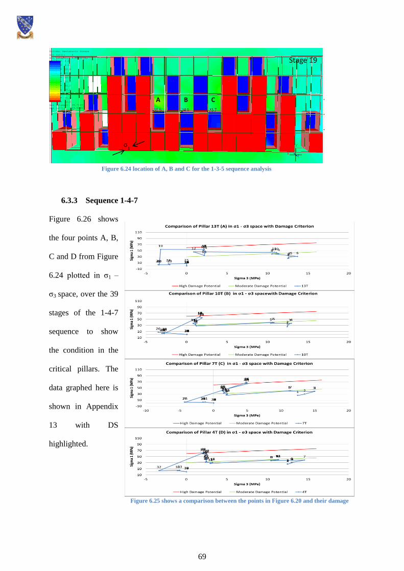
69
6.3.3 Sequence 1-4-7
Figure 6.26 shows
the four points A, B,
C and D from Figure
6.24 plotted in σ1 –
σ3 space, over the 39
stages of the 1-4-7
sequence to show
the condition in the
critical pillars. The
data graphed here is
shown in Appendix
13 with DS
highlighted.
Stage 19
σ1
A C B
Solids: Deviatoric Stress
0.0
5.0
10.0
15.0
20.0
25.0
30.0
35.0
40.0
45.0
50.0
min (all): 0
min (stage): 0.00102299
max (stage): 38.7133
max (all): 49.5085
Figure 6.24 location of A, B and C for the 1-3-5 sequence analysis
Figure 6.25 shows a comparison between the points in Figure 6.20 and their damage
over 40 stages.

70
As shown in RT1 analysis in previous sections, the damage in the critical pillars is mainly
minimal in the early stages. It then spikes as adjacent stopes are mined with the channelling
of stress through the tertiary pillars. Stage 10 through to stage 30 sees damage being
sustained at these four points. This is the earliest of the sequences to show damage and this is
sustained for the longest period of 20 stages. It is important to note that Points C and D
present the highest damage potential in this analysis with values of 42.9% and 40.6% of UCS
150 (or >60MPa). These four points show how RT 1 damage is sustained in the same place in
each row within the critical pillars. These other rows are investigated more fully along with
the other RTs in Appendix 9.
A final consideration that must be noted is the stages that present tension in σ3 stress. This
usually occurs three stages before the tertiary stope is mined. This does not produce a
significant DS but does show as de-stressed in Figure 6.25. This is the same condition in
which RT2 and RT3 produces yield as shown in the continuous and 1-3-5 analysis.
Solids: Deviatoric Stress
0.0
5.3
10.6
15.9
21.2
26.5
31.8
37.1
42.4
47.7
53.0
min (all): 0
min (stage): 0.000435034
max (stage): 37.0716
max (all): 52.9173
Stage 16
T16 T13 T10 T7 T4
σ1
A D C B
Figure 6.26 location of A, B, C and D for the 1-4-7 sequence analysis

71
6.3.4 Sequence 1-5-9
Figure 6.27 shows the four points A, B, C and D from Figure 6.28 plotted in σ1 – σ3 space,
over the 43 stages of the 1-5-9 sequence to show the condition in the critical pillars. The data
graphed here is shown in Appendix 14 with DS highlighted.
Figure 6.27 shows a comparison between the points in Figure 6.20 and their damage over
40 stages.
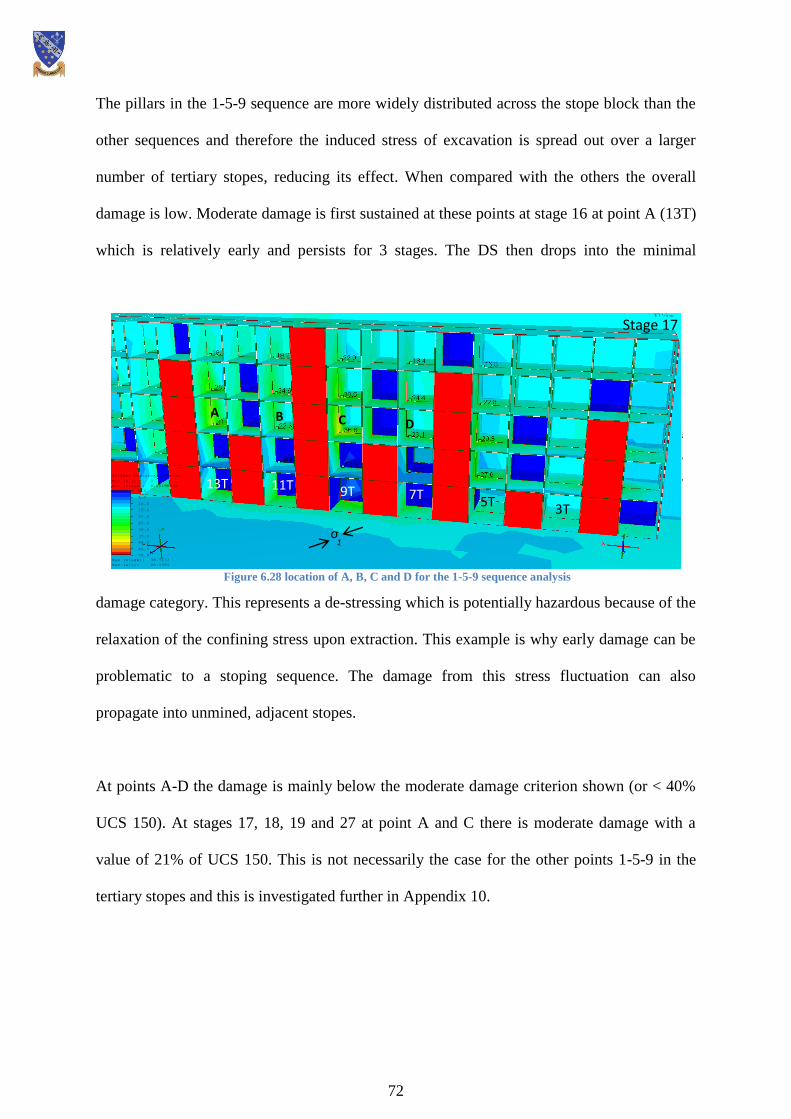
72
The pillars in the 1-5-9 sequence are more widely distributed across the stope block than the
other sequences and therefore the induced stress of excavation is spread out over a larger
number of tertiary stopes, reducing its effect. When compared with the others the overall
damage is low. Moderate damage is first sustained at these points at stage 16 at point A (13T)
which is relatively early and persists for 3 stages. The DS then drops into the minimal
damage category. This represents a de-stressing which is potentially hazardous because of the
relaxation of the confining stress upon extraction. This example is why early damage can be
problematic to a stoping sequence. The damage from this stress fluctuation can also
propagate into unmined, adjacent stopes.
At points A-D the damage is mainly below the moderate damage criterion shown (or < 40%
UCS 150). At stages 17, 18, 19 and 27 at point A and C there is moderate damage with a
value of 21% of UCS 150. This is not necessarily the case for the other points 1-5-9 in the
tertiary stopes and this is investigated further in Appendix 10.
Figure 6.28 location of A, B, C and D for the 1-5-9 sequence analysis
Solids: Deviatoric Stress
0.0
5.0
10.0
15.0
20.0
25.0
30.0
35.0
40.0
45.0
50.0
min (all): 0
min (stage): 0.00102299
max (stage): 38.7133
max (all): 49.5085
Stage 17
13T 11T 9T 7T 5T 3T
A D C B
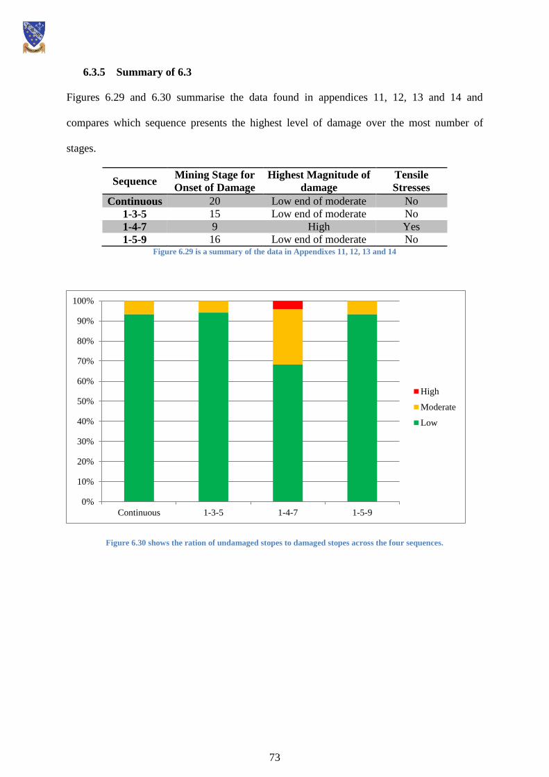
73
6.3.5 Summary of 6.3
Figures 6.29 and 6.30 summarise the data found in appendices 11, 12, 13 and 14 and
compares which sequence presents the highest level of damage over the most number of
stages.
Sequence Mining Stage for
Onset of Damage
Highest Magnitude of
damage
Tensile
Stresses
Continuous 20 Low end of moderate No
1-3-5 15 Low end of moderate No
1-4-7 9 High Yes
1-5-9 16 Low end of moderate No Figure 6.29 is a summary of the data in Appendixes 11, 12, 13 and 14
Figure 6.30 shows the ration of undamaged stopes to damaged stopes across the four sequences.
0%
10%
20%
30%
40%
50%
60%
70%
80%
90%
100%
Continuous 1-3-5 1-4-7 1-5-9
High
Moderate
Low

74
6.4 Damage with Increased Depth of Excavation
The query line along the front of the stope block
in Figure 6.32 is situated 60m up the face and
15m away from the stope boundary. It
demonstrates low values throughout the
sequence at their highest ~13MPa in the middle
of the stopes and 22.5MPa at the corners. This is
within the minimal damage bracket so therefore
this region in both the HW and FW can be
considered low risk. The stress at depth
considered here is roughly equivalent to 400m of
overburden, see Bridges (2007) in Sharp (2011)
in Figure 6.31. This shows the relationship between depth and the values of σ1, σ2 and σ3. At
400m the field stresses discussed in section 3.1 and at 800m they are 39MPa, 31MPa and
27Mpa. By increasing the virgin stress field for the same sequence there should be an
increase in the damage observed. It will indicate the extent to which damage will be sustained
in the HW and FW.
The two queried points on top of each excavation in Figure 6.8 show how the damage
focusses on top of the excavation. The Figure aims to look at the damage in the -Z direction
so contours showing below the stope block as concealed by this XZ plane. Figure 6.33 shows
the damage in the crown and rock below the stope. It is important to note that the queried
point, value of 24.9MPa, lies 40m below the fill of row one. Values however in the stope
backs of row 5 show a DS of 60MPa and 63MPa with the maximum for this model being
65MPa.
Figure 6.31 shows the magnitude of principal
stress versus depth (Bridges, 2007 in Sharp
2011).

75
This is classified as high damage potential and would therefore experience high damage
within the stope block as well as high moderate damage within the block. Therefore any
development or further stoping activity must consider damage implications before entering
this area.
The 19 data points
along the query line
present different results
for the 400m and 800m
depth analysis. The
average value for the
400m and 800m are
Stage 40 – Depth 400m Max: 43.4MPa
Solids: Deviatoric Stress
0.0
5.6
11.2
16.8
22.4
28.0
33.6
39.2
44.8
50.4
56.0
min (all): 0.000147126
min (stage): 0.00217837
max (stage): 43.9678
max (all): 55.4822
σ1
Stage 40 – Depth 800m
σ1
Solids: Deviatoric Stress
0.0
7.0
14.0
21.0
28.0
35.0
42.0
49.0
56.0
63.0
70.0
min (all): 0.000216431
min (stage): 0.00374053
max (stage): 65.0252
max (all): 84.9534
Max: 65MPa
Figure 6.32 shows change in DS at stage 4 at 400m and 800m depth
Stage 40 – Depth 800m
σ1
Solids: Deviatoric Stress
0.0
7.0
14.0
21.0
28.0
35.0
42.0
49.0
56.0
63.0
70.0
min (all): 0.000216431
min (stage): 0.00374053
max (stage): 65.0252
max (all): 84.9534
Max: 65MPa
Figure 6.33 shows stage 40 under 800m metre depth conditions to highlight
potential damaged regions above and below the excavated area.
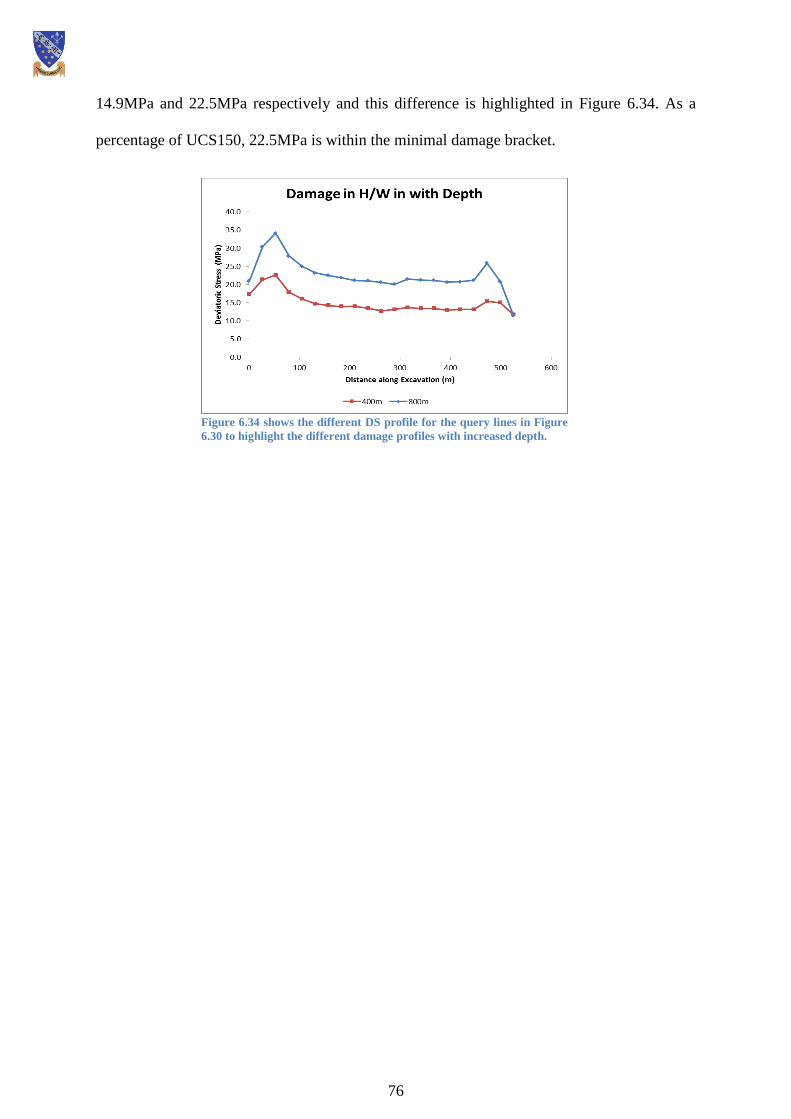
76
14.9MPa and 22.5MPa respectively and this difference is highlighted in Figure 6.34. As a
percentage of UCS150, 22.5MPa is within the minimal damage bracket.
Figure 6.34 shows the different DS profile for the query lines in Figure
6.30 to highlight the different damage profiles with increased depth.

77
7. Discussion of Results
The results of the section 6 address the aims set out in section 1.2. RS3 was used to analyse
four different stope extraction sequences in terms of excavation depth, stress and damage
both within the stope block and the HW and FW. An in depth appraisal of every permutation
of the sequences for each stope was too extensive for a study of this nature so therefore the
worst case regions of damage affected areas were identified and analysed. This section will
take the objectives and discuss how these were addressed and the implications that stem from
the findings.
7.1 Objective 1
Compare the sequences in terms of overall damage experienced within critical stopes
For a viable comparison of the four sequences a standardised sampling strategy must be used
so that there can be a benchmark from which to compare the sequences. This has been
performed as shown in section 6.1. It was decided that the worst damage produced in each
case, was in the closure pillars and each of these would be tested at the central point in each
stope.
The results produced show that the lowest overall damage is experienced within the tertiary
pillars of 1-5-9 with a DS of 12.0MPa. The worst overall damage is 14.0MPa in the
continuous sequence. When assessed however in the specific regions of sections 6.3 it shows
that the 1-4-7 sequence has the highest DS and the earliest onset of damage. The 1-4-7
sequence also contains σ3 tension stress (Appendix 14) which further weakens the rock mass.
The difference between the two is so negligible that there is no significantly favourable low
damage scenario that is offered by any one of the sequences. Therefore it can be concluded
that this way of comparing the sequences is not effective and the analysis of specific regions
in each sequence is a more effective way of sequence selection.

78
7.2 Objective 2
Assess the impact of increased depth on the stability of the sequences:
This was carried out in section 6.4 using the continuous sequence. It found that the principal
stresses at 800m of σ1, σ2 and σ3 were 39MPa, 31MPa and 27Mpa respectively. Under this
stress condition, almost double of original 400m depth stress conditions, the DS was found to
be in the high damage potential category (>0.4 of UCS 150 or >60MPa deviation). Although
the maximum value is not representative of the whole stope section it indicates that the
average damage level would rise considerably with a deeper excavation.
Although the assessment of rock damage in the HW deemed the maximum DS to be 35MPa
(moderate damage) with an average of 24MPa (minimal damage) this is almost double the
value found for the 400m excavation.
7.3 Objective 3
7.3.1 Damage: Identify and investigate damaged regions unique to each sequence
within the stope block.
Each sequence was examined under a number of different mediums for assessing stability,
stress concentration and damage. The specific regions are noted in each of the analysis
sections that demonstrate the location and the severity of the damage sustained in each
section.
7.3.1.1 Continuous Sequence:
Points A-E in Figure 3.1.4 show the worst affected regions in the continuous sequence each
with different values at each stage. The damage level never exceeded 60MPa out of the
moderate damage bracket with maximum values of 55MPa and 53MPa within the stope

79
block. This damage can be mitigated with the use of bolting and shotcrete in drill drives and
cross cuts when entering the stope area. The location of the highest stress can be accurately
determined from the model and can be used when mining the area in question.
The closure pillars in each of the sequences are the regions found to contain the highest level
of damage. Due to the virgin stress field this presented the damage in the side wall of the
neighbouring stope see 11P in Figure
7.1. Looking at panel 2 in Figure 7.1 it
is clear the concentration is in the
bottom left corner of row 5 in pillar
10S.
Each sequence found a similar result for
the location of the DS in the left-hand sidewall of the neighbouring stope. It is caused by the
orientation of the principal stresses diverting around the filled stopes and concentrating σ1
stress. It was found that the σ3 stress either decreased or remained constant which caused the
DS to increase as highlighted in the graphs in Figure 6.8. The location of this damage can
affect the filled neighbouring stopes creating slabbing or sloughing which in turn would
cause dilution of the product rock upon blasting but the extent to which this would occur
cannot be determined from this project.
7.3.1.2 Sequence 1-3-5:
The 1-3-5 sequence is the first use of the primary-secondary technique for stoping. The
primary stopes are mined first leaving the secondary stopes as pillars that act as channels
through which the displaced principal stress can ‘flow’ through. The new channels focus the
σ1 stress whilst the σ3 stress is diverted around the stope block by the peaks of the primary
Solids: Deviatoric Stress
0.0
5.6
11.2
16.8
22.4
28.0
33.6
39.2
44.8
50.4
56.0
min (all): 0.000102962
min (stage): 0.00725663
max (stage): 49.9524
max (all): 55.2139
D
E
F
G
Stage 34
X
3P
8S 9P 10S 11P 12S 13P
Y
Z
Figure 7.1 shows panel 2 and where the DS was at its maximum.
80
pillars. The highest DS that is produced from this sequence is also 55MPam the same as the
continuous sequence. Minimal damage is sustained until the secondary stopes are mined
which causes a further concentration of σ1 stress in the pendant pillars created from the
closure of the bottom row of stopes. The stope-specific location of the stress concentration
does not differ from the continuous sequence but the pillars affected change.
The worst affected areas in the 1-3-5 sequence are the secondary stopes 4S, 8S, 10S, 12S and
16S. This is generally the case however stress shadowed pendant pillars, such as 6S and 14S
(Figure 6.18), show how the DS analysis is limited. Under plastic analysis these pendant
pillars show yielded elements within these pillars in row 3. Here, there is a σ1 and σ3
relaxation which is different to the damaged regions shown by DS where it is usually just a σ1
concentration that creates the damage. The damage caused here is from tension failure and
low confining stresses.
7.3.1.3 Sequence 1-4-7:
The 1-4-7 sequence uses tertiary stopes for the first time and there these are the last stopes
left in the sequence and through which the majority of the principal stress diverts. The
maximum DS found within the sequence was 52MPa (moderate damage), lower than the
previous two sequences.
The worst affected stopes were the tertiary pillars T7, T10, T13 and T16 with values of
~45MPa (moderate damage) under DS analysis. The rear top edge of panel 1 stopes is where
σ1 and σ2 stress concentrates as it ‘flows’ around the filled stopes. This means that the σ1
stress is contributing here instead of a low confining stress.
There are no regions which are as significantly de-stressed as the example in the 1-3-5
81
sequence however in each pillar there are vulnerable stages that, with the vertical advance of
panel 1 become systematically de-stressed. It is at this stage that damage, not shown up by
DS analysis, occurs. This was picked up by the plastic analysis and shown to be vulnerable
by yielded elements at these positions within these tertiary pillars.
7.3.1.4 Sequence 1-5-9:
This sequence also uses a tertiary set of stopes but only one central lead primary stope. Over
the widest area and with more tertiary stopes than the 1-4-7 sequence the in situ stress can
dissipate over a larger area and through more filled stopes. This is one of the reasons for the
1-5-9 sequence having the lowest DS of all the sequence at 49MPa.
Therefore the tertiary pillars experience the worst damage conditions as the pillars are closed
out. Again, due to the field stress orientation the damage is mainly found to affect the bottom
left corner of the tertiary stopes in panel 2.
The plastic analysis of the 1-5-9 sequence showed extensive damage within the tertiary
pillars and post-closure, the pendant pillars. These stopes suffered the same de-stressing with
the advance of panel 1 as the previous sequences and therefore would experience damage in
these stopes due to tension stress or low confinement as opposed to high σ1 concentration.
7.3.2 Ascertain the level of damage within the HW and FW
The HW and FW at no stage present any signs of critical DS so therefore under elastic rock
conditions no deterioration of the rock mass is observed. Under σ3 contouring however, large
areas of low σ3 stress are seen in the HW and FW. This comes from the vertical σ3 stress
diverting around the stope block concentrating at the edges but reducing at the sides.
Consequently the plastic analysis reveals yielded elements as a result of this low confining

82
stress in this region. The plastic analysis is not necessarily an accurate depiction of how the
rock will react because the rock is likely to have an elastic reaction but the yielded elements
highlight the regions in which the HW and FW are vulnerable to damage.
This has operational considerations because the HW and FW drives are key infrastructure for
access and ore movement that must remain stable as semi-permanent openings for the
duration of the stope block. Cross cuts and drill drives are also created from within the HW
and FW that provide access to the stopes so any damage could cause slabbing along drives,
block fallout, floor closure or in particularly high stress environments, rockbursts.
83
7.4 Objective 4
Assess the sequences with regard to the stage in which the damage begins to occur.
Section 6.3 assesses the stage of notable damage initiation in each of the four sequences. It
uses 3 or 4 points in row 2 of critical pillars of each sequence. Row two is early enough to be
an early indicator and high enough in the stope block to experience significant damage that
row 1 would not get.
Graphs plotted induced stress in σ1 – σ3 space and set the points against damage potential
criterion noting when the damage was sustained. This showed that the 1-4-7 sequence had the
most severe (DS-61MPa in tertiary pillar 4T) and also the earliest and longest period of high
damage potential as DS doubled over 12 stages. Normally sequences with tertiary stopes
experience damage later than primary-secondary sequences. This is likely to be a
consequence of the model being run with two panels. The induced stresses force the stress to
concentrate around the fill in panel 1 and cause damage in the tertiary stopes in panel 2. If
this is the case there would be a simpler damage result if a singular panel was run and the
damage would appear later in the sequence.
The 1-5-9 sequence experiences the least number of stages with high damage potential which
is in keeping with the norm for tertiary sequences. This is because there are nine tertiary
pillars that conduct the induced stress, spreading the loading and reducing damage.
84
8. Limitations
This section will include a list of elements that have not been able to be considered or
modelled in this project. The scale of this thesis could not include these elements without
detracting from the original aim of the project which was to assess damage in popular stope
sequencing options.
8.1 Jointing
Few rock masses in the world are fully competent and homogenous. Joint sets, bedding
planes faults create lines of weakness that create damage and instability in most mining
operations. The modelled rock conditions used here did not consider the influence of jointing
because the stress results would have been too complex to extract insightful conclusions for
such broad project.
8.2 DS versus low σ3 confining stress as method of finding damage
This was explored in section 2.1.1 and illustrated in Figure 6.18. The DS was the main way in
which damage was identified and compared throughout this investigation. Because it uses the
difference between σ1 and σ3 it fails to recognise the vulnerability of the rock when both σ1
and σ3 are experiencing low values as the DS shows stable or minimal damage. It does not
however consider tension failure or low confinement coupled with low σ1 and σ2.
8.3 Single Panel
A single panel of stopes would have been a useful tool for assessing the sequence for its basic
induced stress paths and damage results.
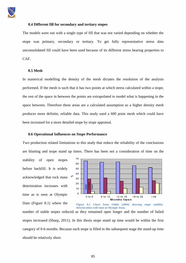
85
8.4 Different fill for secondary and tertiary stopes
The models were run with a single type of fill that was not varied depending on whether the
stope was primary, secondary or tertiary. To get fully representative stress data
unconsolidated fill could have been used because of its different stress bearing properties to
CAF.
8.5 Mesh
In numerical modelling the density of the mesh dictates the resolution of the analysis
performed. If the mesh is such that it has two points at which stress calculated within a stope,
the rest of the space in between the points are extrapolated to model what is happening in the
space between. Therefore these areas are a calculated assumption so a higher density mesh
produces more definite, reliable data. This study used a 600 point mesh which could have
been increased for a more detailed stope by stope appraisal.
8.6 Operational Influences on Stope Performance
Two production related limitations to this study that reduce the reliability of the conclusions
are blasting and stope stand up times. There has been not a consideration of time on the
stability of open stopes
before backfill. It is widely
acknowledged that rock mass
deterioration increases with
time as is seen at Olympic
Dam (Figure 8.1) where the
number of stable stopes reduced as they remained open longer and the number of failed
stopes increased (Sharp, 2011). In this thesis stope stand up time would be within the first
category of 0-6 months. Because each stope is filled in the subsequent stage the stand-up time
should be relatively short.
Figure 8.1 Chart from Oddie (2004) showing stope stability
deterioration with time at Olympic Dam.

86
There has been no consideration of blasting effects on the stability. Blasting often leads to the
degradation of the rock mass by blasting-induced fractures. Major discontinuities such as
faults, shears and dykes usually have very low shearing strength. Vibration and disturbance
caused from the blasting process can further reduce the shear strength of these discontinuities,
initiating failure.
87
9. Conclusion and Future Work
9.1 Conclusion
The induced stress pattern during an active stoping sequence is in constant flux as stress finds
a different path around combinations of rock and backfill. The sequences employed are
designed to be as unobtrusive as possible manipulating the virgin stress field to divert
concentrations into the abutments ensuring minimal damage is sustained at all times within
the stope area.
The nature of the four sequences is such that a standardised comparison produced no
significant preferential difference in damage; therefore a more biased approach was taken.
This took the form of a more rigorous appraisal of the worst case (stope) scenarios in each
sequence, focussing on the regions most at risk of damage. As a result, a more targeted
approach identified four mechanisms that create damage both within the stope block and in
the HW and FW. These included damage stemming from high DS exceeding standardised
damage criterion and deterioration of the rockmass brought about by low confining stress in
certain stope arrangements.
These failure mechanisms are common to all four sequences and they vary according to the
shape created by the each sequence channelling induced stresses into stress window of the
closure pillars and the abutments. In Primary-Secondary sequences the damage is found
largely in the secondaries and in Primary-Secondary-Tertiary sequences the damage is found
in the Tertiary stopes. Localised damage however will occur in the sidewall of stopes with
adjacencies to these critical stopes.
The location of damage found in this thesis can be usefully applied into an active stoping

88
operation to better understand the global stress redistribution when employing each sequence.
It will enable the mine engineer to identify problematic stopes so that measures can be
employed to maintain safety and maintain operational efficiency rather than be constrained
by unforeseen damage that affects productivity.
9.2 Future Work
Stope Widths
As mentioned in the introduction, stope width can be varied according to the planned cash
flow for the mine. This has not been modelled in this study and is an important factor to
consider when using these conclusions. If the stope widths were altered this would alter the
stress paths through the stope block. Thinner stopes would present more damage and wider
ones would have less damage. If secondary or tertiary pillars in this project were made
thinner there would be greater damage and yield as these are the stopes that sustain the most
damage.
Crown, Sill and Rib pillars
Many operations use pillars between rows of stopes that are left in place. Sill pillars and
crown pillars are used to separate stoping zones vertically and Rib pillars horizontally. The
use of these pillars is determined by the geotechnical environment and the stresses induced by
mining and can be very useful to dissipate stress in a higher stress environment. Perhaps this
would be an option at deeper levels of an operation. If this was modelled are clearer picture
of the range of options for stress management could be achieved.
Jointing
This has already been discussed in the limitations section however further work modelling
the effect of jointing would be useful to visualise with a mine specific joint set.
89
10. References
Bieniawski, Z. T. (1979). The geomechanics classification in rock engineering
applications. In 4th ISRM Congress.
Board, M. Brummer, R. Seldon, S., (2001). Use of numerical modelling for mine
design and evaluation. In: Hustrulid WA, Bullock RL, editors. Underground
mining methods: engineering fundamentals and international case studies. Littleton,
Colo: Soc Mining Metall Explor. pp. 482–91.
Bridges, M.C. (2007). In situ stress field for Olympic Dam, Australian Mining
Consultants.
Bywater S., R. Cowling and B. Black, (1985). Stress measurements and analysis
for mine planning, Procc. Fifth ISRM Congress, Melbourne Australia, D29-D37.
Ghasemi, Y. (2012). Numerical studies of mining geometry and extraction
sequencing in Lappberget, Garpenberg. Luleå University of Technology
Hoek, E., 1968. Brittle failure of rock. In Rock mechanics in engineering practice
(Ed. K. G. Stagg and O. C. Zienkiewicz), pp. 99–124. JohnWiley and Sons Ltd.,
London.
Hoek, E., Kaiser, P. K., and Bawden, W. F. (2000). Support of underground
excavations in hard rock. CRC Press.
Martin, C. D., Tannant, D. D., Yazici, S., and Kaiser, P. K. (1999). Stress path
and instability around mine openings. In Proc. 9th, ISRM Congress on Rock
Mechanics (Vol. 1, pp. 311-315).
Mathews, K. E., E. Hoek, D. C.Wyllie and S. B.V. Stewart, (1981). Prediction of
stable excavations for mining at depth below 1000 metres in hard rock. CANMET
Report DSS Serial No. OSQ80- 00081, Natural Resources Canada, Ottawa.
Oddie, M. E., 2004. Minimum Ground Support Requirements for Development
90
Headings at Olympic Dam, Australian Mining Consultants, Melbourne.
Oddie, M. E., and Pascoe, M. 2005. Stope Performance at Olympic Dam Mine
Poole, J. R. and Mutton, B. K., (1977). Applied structural geology in cut and fill
stoping operations at Mt Isa, The Aus. IMM, Broken Hill Branch, Underground
Operators Conference, pp.123-128 in Tavakoli, M. (1994). Underground metal
mine crown pillar stability analysis.
Potvin, Y., M. R. Hudyma and H. D. S. Miller, (1989). Design guidelines for open
stope support. Bull. Can. Min. Metall., 82(926):53–62.
Potvin, Y., and Hudyma, M. (2000). Open stope mining in Canada. Procc
MassMin 2000.
Rocscience, (2014). https://www.rocscience.com/products/16/RS3. Accessed
05.08.14
Sharp, J. (2011). Applicability of the Mathews Stability Method to Open Stope
Stability Assessment at Olympic Dam Mine.
Stephan. G. in Darling, P. (Ed.). (2011). SME mining engineering handbook (Vol.
1). SME.
Stillberg, B. L., 1984. Open Stope design at the research mine in Kiruna, Sweden,
design and performance of underground excavations, London, pp.237 - 283
Villaescusa, E. (2000). A review of sublevel stoping. MassMin2000, 577-590.
Villaescusa, E. (2003). Global Extraction Sequences in Sublevel Stoping. In MPES
2003, Conference Kalgoorlie April 2003.
Villaescusa, E. (2014). Geotechnical Design for Sublevel Open Stoping. CRC Press.

11. Appendices
11.1 Appendix 1
Figure 11.1 shows the input data for the Mathews Stability Method carried out by Sharp (2011). It has been used to
provide values for N’ in the crown and walls of the modelled stopes.
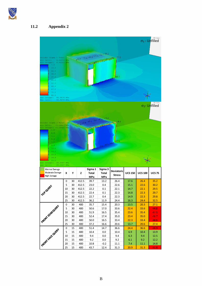
B
11.2 Appendix 2
Solids: Sigma 1 Total
7.5
15.0
22.5
30.0
37.5
45.0
52.5
60.0
67.5
75.0
82.5
min (all): 8.64203 MPa
min (stage): 8.64203 MPa
max (stage): 66.9674 MPa
max (all): 66.9674 MPa
Solids: Sigma 3 Total
-1.4
0.9
3.1
5.4
7.7
9.9
12.2
14.4
16.6
18.9
21.1
min (all): -1.16447 MPa
min (stage): -1.16447 MPa
max (stage): 20.3547 MPa
max (all): 20.3547 MPa
σ3- Unfilled
σ1 - Unfilled
X Y Z
Sigma 1
Total
MPa
Sigma 3
Total
MPa
Deviatoric
StressUCS 150 UCS 100 UCS 75
TOP Q
UERY
0 30 412.5 39.7 13.2 26.4 17.6 26.4 35.2
5 30 412.5 23.0 0.4 22.6 15.1 22.6 30.2
10 30 412.5 22.2 0.1 22.1 14.7 22.1 29.5
15 30 412.5 22.4 0.1 22.3 14.8 22.3 29.7
20 30 412.5 22.7 0.4 22.3 14.9 22.3 29.8
25 30 412.5 36.2 11.9 24.4 16.3 24.4 32.5
TOP Q
UERY
FRONT ED
GEQUERY
0 30 400 35.7 15.4 20.3 13.5 20.3 27.1
5 30 400 50.6 17.0 33.6 22.4 33.6 44.8
10 30 400 51.9 16.5 35.4 23.6 35.4 47.1
15 30 400 52.4 17.4 35.0 23.4 35.0 46.7
20 30 400 50.0 16.5 33.4 22.3 33.4 44.6
25 30 400 37.2 16.6 20.6 13.7 20.6 27.4FR
ONT EDGEQUER
Y
FRONT FA
CE QUER
Y0 15 400 51.4 14.7 36.6 24.4 36.6 48.9
5 15 400 10.4 0.0 10.4 6.9 10.4 13.9
10 15 400 9.4 0.0 9.4 6.3 9.4 12.5
15 15 400 9.2 0.0 9.2 6.1 9.2 12.2
20 15 400 10.8 -0.2 11.1 7.4 11.1 14.8
25 15 400 43.7 12.4 31.3 20.9 31.3 41.8FR
ONT FACE
QUERY
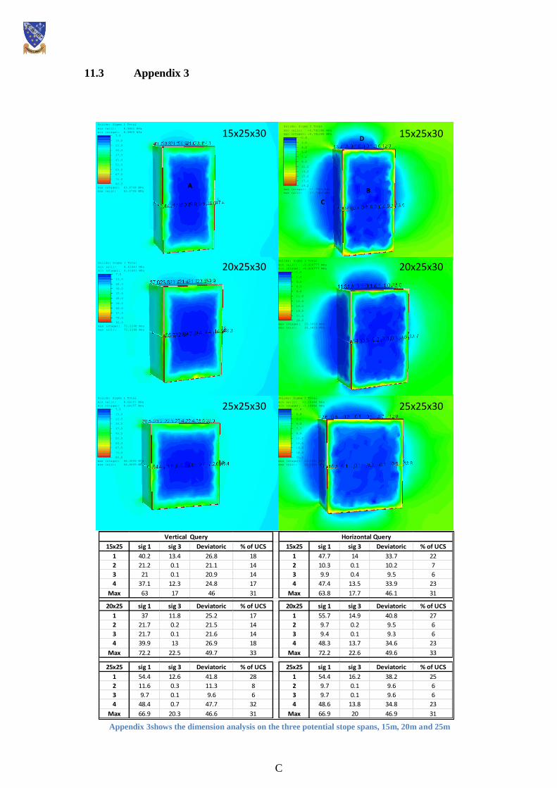
C
11.3 Appendix 3
Solids: Sigma 3 Total
-0.8
1.2
3.2
5.2
7.2
9.2
11.2
13.2
15.2
17.2
19.2
min (all): -0.791386 MPa
min (stage): -0.791386 MPa
max (stage): 17.7364 MPa
max (all): 17.7364 MPa
Solids: Sigma 3 Total
-1.4
0.9
3.1
5.4
7.7
9.9
12.2
14.4
16.6
18.9
21.1
min (all): -1.16466 MPa
min (stage): -1.16466 MPa
max (stage): 20.3552 MPa
max (all): 20.3552 MPa
Solids: Sigma 1 Total
7.5
15.0
22.5
30.0
37.5
45.0
52.5
60.0
67.5
75.0
82.5
min (all): 8.64157 MPa
min (stage): 8.64157 MPa
max (stage): 66.9699 MPa
max (all): 66.9699 MPa
Solids: Sigma 1 Total
7.5
15.0
22.5
30.0
37.5
45.0
52.5
60.0
67.5
75.0
82.5
min (all): 8.9805 MPa
min (stage): 8.9805 MPa
max (stage): 63.8748 MPa
max (all): 63.8748 MPa
Solids: Sigma 3 Total
-1.0
1.5
4.0
6.5
9.0
11.5
14.0
16.5
19.0
21.5
24.0
min (all): -0.626777 MPa
min (stage): -0.626777 MPa
max (stage): 22.5818 MPa
max (all): 22.5818 MPa
Solids: Sigma 1 Total
7.5
15.0
22.5
30.0
37.5
45.0
52.5
60.0
67.5
75.0
82.5
min (all): 8.61843 MPa
min (stage): 8.61843 MPa
max (stage): 72.2298 MPa
max (all): 72.2298 MPa
A B
C
D 15x25x30 15x25x30
20x25x30 20x25x30
25x25x30 25x25x30
Appendix 3shows the dimension analysis on the three potential stope spans, 15m, 20m and 25m
15x25 sig 1 sig 3 Deviatoric % of UCS 15x25 sig 1 sig 3 Deviatoric % of UCS
1 40.2 13.4 26.8 18 1 47.7 14 33.7 22
2 21.2 0.1 21.1 14 2 10.3 0.1 10.2 7
3 21 0.1 20.9 14 3 9.9 0.4 9.5 6
4 37.1 12.3 24.8 17 4 47.4 13.5 33.9 23
Max 63 17 46 31 Max 63.8 17.7 46.1 31
20x25 sig 1 sig 3 Deviatoric % of UCS 20x25 sig 1 sig 3 Deviatoric % of UCS
1 37 11.8 25.2 17 1 55.7 14.9 40.8 27
2 21.7 0.2 21.5 14 2 9.7 0.2 9.5 6
3 21.7 0.1 21.6 14 3 9.4 0.1 9.3 6
4 39.9 13 26.9 18 4 48.3 13.7 34.6 23
Max 72.2 22.5 49.7 33 Max 72.2 22.6 49.6 33
25x25 sig 1 sig 3 Deviatoric % of UCS 25x25 sig 1 sig 3 Deviatoric % of UCS
1 54.4 12.6 41.8 28 1 54.4 16.2 38.2 25
2 11.6 0.3 11.3 8 2 9.7 0.1 9.6 6
3 9.7 0.1 9.6 6 3 9.7 0.1 9.6 6
4 48.4 0.7 47.7 32 4 48.6 13.8 34.8 23
Max 66.9 20.3 46.6 31 Max 66.9 20 46.9 31
Vertical Query Horizontal Query
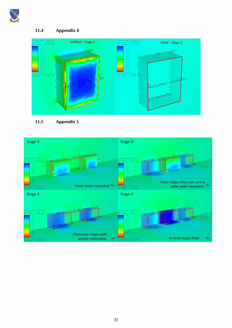
D
11.4 Appendix 4
11.5 Appendix 5
Solids: Sigma 1 Effective
7.0
13.3
19.6
25.9
32.2
38.5
44.8
51.1
57.4
63.7
70.0
min (all): 8.64203 MPa
min (stage): 8.64203 MPa
max (stage): 66.9674 MPa
max (all): 66.9674 MPa
Solids: Sigma 1 Effective
7.0
13.3
19.6
25.9
32.2
38.5
44.8
51.1
57.4
63.7
70.0
min (all): 8.64203 MPa
min (stage): 19.37 MPa
max (stage): 25.9148 MPa
max (all): 66.9674 MPa
Unfilled – Stage 1 Filled – Stage 2
Solids: Sigma 1 Effective
0.0
7.5
15.0
22.5
30.0
37.5
45.0
52.5
60.0
67.5
75.0
min (all): -0 MPa
min (stage): 11.133 MPa
max (stage): 46.567 MPa
max (all): 59.605 MPa
Solids: Sigma 1 Effective
0.0
7.5
15.0
22.5
30.0
37.5
45.0
52.5
60.0
67.5
75.0
min (all): -0 MPa
min (stage): 7.95869 MPa
max (stage): 39.6075 MPa
max (all): 59.605 MPa
Solids: Sigma 1 Effective
0.0
7.5
15.0
22.5
30.0
37.5
45.0
52.5
60.0
67.5
75.0
min (all): -0 MPa
min (stage): 10.0072 MPa
max (stage): 59.605 MPa
max (all): 59.605 MPa
Solids: Sigma 1 Effective
0.0
7.5
15.0
22.5
30.0
37.5
45.0
52.5
60.0
67.5
75.0
min (all): -0 MPa
min (stage): -0 MPa
max (stage): 47.3145 MPa
max (all): 59.605 MPa
Stage 1 Stage 3
Stage 2 Stage 4
Filled outer stopes with granite centre pillar
Outer stopes excavated
All three stopes filled
Outer stopes filled with central pillar under excavation.
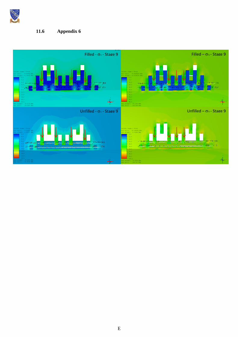
E
11.6 Appendix 6
Solids: Sigma 3 Total
-2.0
0.0
2.0
4.0
6.0
8.0
10.0
12.0
14.0
16.0
18.0
min (all): -3.61833 MPa
min (stage): -1.90797 MPa
max (stage): 16.2326 MPa
max (all): 21.8718 MPa
Solids: Sigma 3 Total
-2.0
0.3
2.5
4.8
7.0
9.3
11.5
13.8
16.0
18.3
20.5
min (all): -3.90954 MPa
min (stage): -1.79612 MPa
max (stage): 18.0174 MPa
max (all): 24.5387 MPa
Solids: Sigma 1 Total
4.5
14.5
24.5
34.5
44.5
54.5
64.5
74.5
84.5
94.5
104.5
min (all): -0.144545 MPa
min (stage): 5.74392 MPa
max (stage): 79.5256 MPa
max (all): 120.197 MPa
Solids: Sigma 1 Total
-2.0
8.0
18.0
28.0
38.0
48.0
58.0
68.0
78.0
88.0
98.0
min (all): -0.0609203 MPa
min (stage): -0.0106205 MPa
max (stage): 75.1192 MPa
max (all): 126.094 MPa
Filled – σ3 - Stage 9
Unfilled – σ3 - Stage 9
Filled - σ1 - Stage 9
Unfilled - σ1 - Stage 9

F
11.7 Appendix 7
Solids: Deviatoric Stress
0.0
5.0
10.0
15.0
20.0
25.0
30.0
35.0
40.0
45.0
50.0
min (all): 0
min (stage): 0.00169025
max (stage): 32.5774
max (all): 49.5085
1-5-9 Comparison – Stage 13 1-4-7 Comparison – Stage 16 Solids: Deviatoric Stress
0.0
6.0
12.0
18.0
24.0
30.0
36.0
42.0
48.0
54.0
60.0
min (all): 0
min (stage): 0.000435034
max (stage): 37.0716
max (all): 52.9173
Solids: Deviatoric Stress
0.0
6.0
12.0
18.0
24.0
30.0
36.0
42.0
48.0
54.0
60.0
min (all): 0.000147126
min (stage): 0.00122631
max (stage): 26.2571
max (all): 55.4822
Shear failure
Tension failure
Critical state failure
Solids: Deviatoric Stress
0.0
6.0
12.0
18.0
24.0
30.0
36.0
42.0
48.0
54.0
60.0
min (all): 0.000102962
min (stage): 0.00125613
max (stage): 39.4193
max (all): 55.2139
1-3-5 Comparison – Stage 19
σ1
σ1 σ
1
σ1
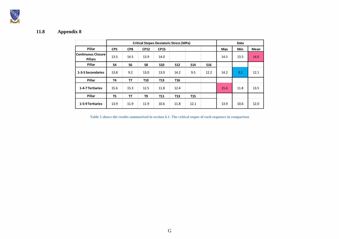
G
11.8 Appendix 8
Table 5 shows the results summarised in section 6.1. The critical stopes of each sequence in comparison
Pillar CP5 CP8 CP12 CP15 Max Min Mean
Continuous Closure
Pillars13.5 14.5 13.9 14.0 14.5 13.5 14.0
Pillar S4 S6 S8 S10 S12 S14 S16
1-3-5 Secondaries 13.8 9.2 13.0 13.0 14.2 9.5 12.2 14.2 9.2 12.1
Pillar T4 T7 T10 T13 T16
1-4-7 Tertiaries 15.6 15.3 12.5 11.8 12.4 15.6 11.8 13.5
Pillar T5 T7 T9 T11 T13 T15
1-5-9 Tertiaries 13.9 11.9 11.9 10.6 11.8 12.1 13.9 10.6 12.0
Critical Stopes Deviatoric Stress (MPa) Data
F
11.9 Appendix 9
11.9.1 Data Analysis from sequence 1-4-7
11.9.1.1 Intra Stope Damage
Figure 11.7 shows stage 16 and 17 of the sequence under DS analysis. In this case, the
tertiary pillars T4, T7, T10, T13 and T16 will be most susceptible to stress and damage
because they are extracted last. Damage will still be seen in the pendant secondary pillars, but
less so.
The excavation of row 1 in T10 and T13 takes place in stage 16 with the subsequent filling of
these in stage 17. Row 1 and 2 in pillar 10 and 13 in panel one have already been filled by
this stage forcing the stress to divert above and below the filled stopes as has been explained
in 3.1 and 3.2 (RT1). The excavation of row 1 in panel two in pillar 10 and 13 causes the row
3 query points location to increase the DS, see Table 5. This is because there is an increase in
the σ1 stress concentration along the back edge of stopes in row 2 to a value of 35MPa and
31MPa in pillars T10 and T13 respectively. These both fall within the threshold of moderate
damage so damage will be sustained. Pillar T7 experiences elevated DS of 34MPa despite no
excavated stope in row 2 of panel 1. This is due to the location of this query point beneath
pillar P8. The σ3 stresses at this point and its contemporary in T10 are 5.7MPa and 6.6MPa
which causes the DS to be higher and damage to be more significant.
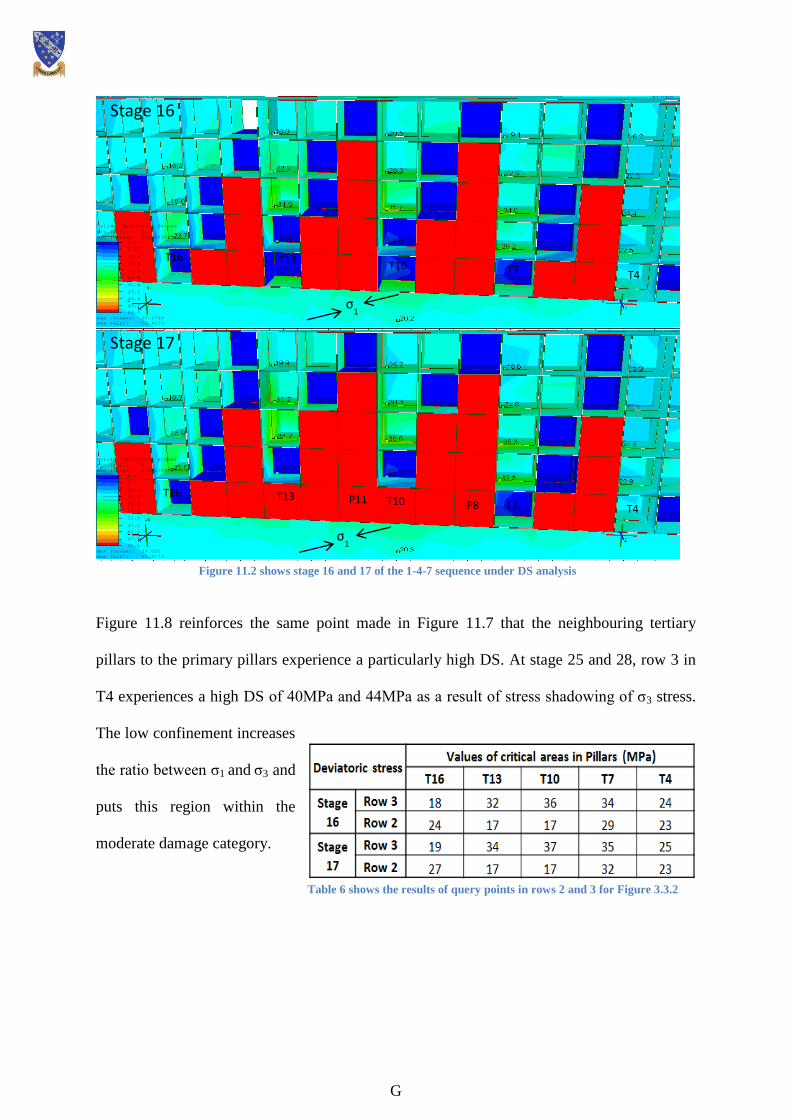
G
Figure 11.8 reinforces the same point made in Figure 11.7 that the neighbouring tertiary
pillars to the primary pillars experience a particularly high DS. At stage 25 and 28, row 3 in
T4 experiences a high DS of 40MPa and 44MPa as a result of stress shadowing of σ3 stress.
The low confinement increases
the ratio between σ1 and σ3 and
puts this region within the
moderate damage category.
Solids: Deviatoric Stress
0.0
5.3
10.6
15.9
21.2
26.5
31.8
37.1
42.4
47.7
53.0
min (all): 0
min (stage): 0.00239979
max (stage): 38.021
max (all): 52.9173
Solids: Deviatoric Stress
0.0
5.3
10.6
15.9
21.2
26.5
31.8
37.1
42.4
47.7
53.0
min (all): 0
min (stage): 0.000435034
max (stage): 37.0716
max (all): 52.9173
Stage 17
Stage 16
σ1
T16 T13 T10 T7 T4
σ1
T16 T13 T10 T7 T4
Figure 11.2 shows stage 16 and 17 of the 1-4-7 sequence under DS analysis
P8 P11
Table 6 shows the results of query points in rows 2 and 3 for Figure 3.3.2
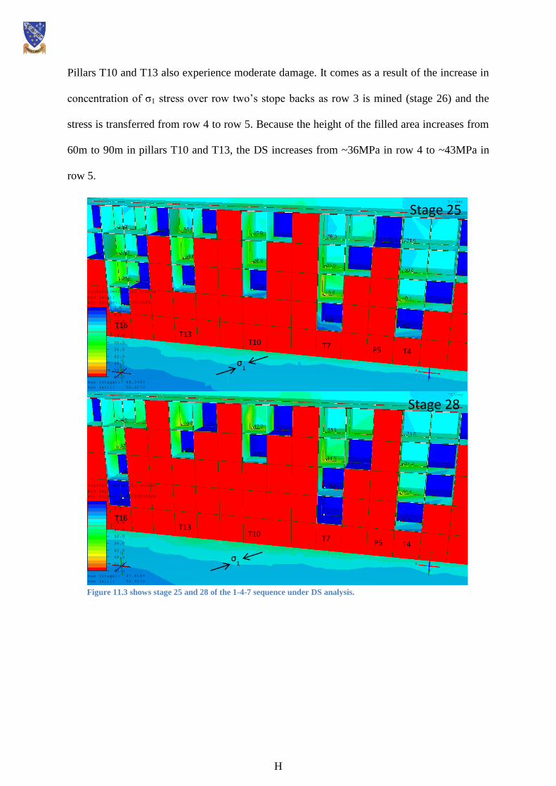
H
Pillars T10 and T13 also experience moderate damage. It comes as a result of the increase in
concentration of σ1 stress over row two’s stope backs as row 3 is mined (stage 26) and the
stress is transferred from row 4 to row 5. Because the height of the filled area increases from
60m to 90m in pillars T10 and T13, the DS increases from ~36MPa in row 4 to ~43MPa in
row 5.
Solids: Deviatoric Stress
0.0
6.0
12.0
18.0
24.0
30.0
36.0
42.0
48.0
54.0
60.0
min (all): 0
min (stage): 0.0044523
max (stage): 46.5493
max (all): 52.9173
Solids: Deviatoric Stress
0.0
6.0
12.0
18.0
24.0
30.0
36.0
42.0
48.0
54.0
60.0
min (all): 0
min (stage): 0.000672376
max (stage): 47.8167
max (all): 52.9173
σ1
σ1
Stage 28
Stage 25
T16 T13
T10 T7 T4
T16 T13
T10 T7
T4
Figure 11.3 shows stage 25 and 28 of the 1-4-7 sequence under DS analysis.
P5
P5
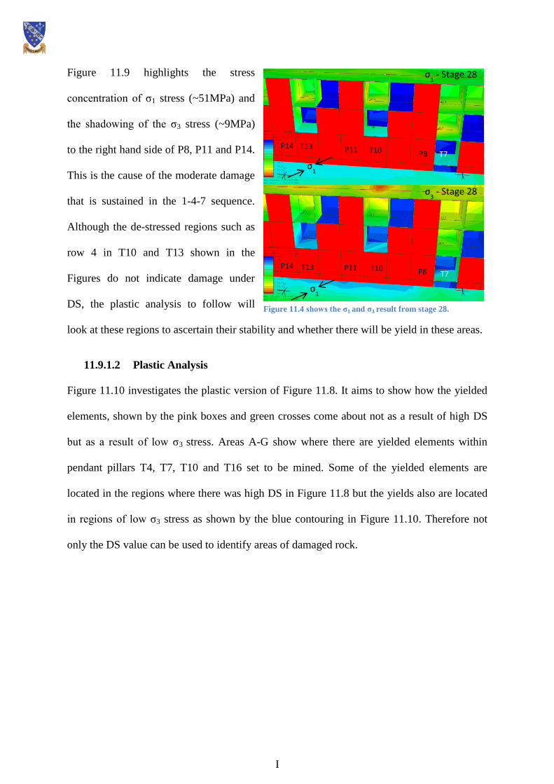
I
Figure 11.9 highlights the stress
concentration of σ1 stress (~51MPa) and
the shadowing of the σ3 stress (~9MPa)
to the right hand side of P8, P11 and P14.
This is the cause of the moderate damage
that is sustained in the 1-4-7 sequence.
Although the de-stressed regions such as
row 4 in T10 and T13 shown in the
Figures do not indicate damage under
DS, the plastic analysis to follow will
look at these regions to ascertain their stability and whether there will be yield in these areas.
11.9.1.2 Plastic Analysis
Figure 11.10 investigates the plastic version of Figure 11.8. It aims to show how the yielded
elements, shown by the pink boxes and green crosses come about not as a result of high DS
but as a result of low σ3 stress. Areas A-G show where there are yielded elements within
pendant pillars T4, T7, T10 and T16 set to be mined. Some of the yielded elements are
located in the regions where there was high DS in Figure 11.8 but the yields also are located
in regions of low σ3 stress as shown by the blue contouring in Figure 11.10. Therefore not
only the DS value can be used to identify areas of damaged rock.
Figure 11.4 shows the σ1 and σ3 result from stage 28.
Solids: Sigma 1 Total
-3.0
4.0
11.0
18.0
25.0
32.0
39.0
46.0
53.0
60.0
67.0
min (all): -0.319389 MPa
min (stage): -0.045017 MPa
max (stage): 58.7055 MPa
max (all): 61.2158 MPa
Solids: Sigma 3 Total
-2.0
0.1
2.2
4.3
6.4
8.5
10.6
12.7
14.8
16.9
19.0
min (all): -4.3779 MPa
min (stage): -1.75694 MPa
max (stage): 18.0548 MPa
max (all): 18.0981 MPa
σ1
T13 T10 T7
T13 T10 T7
σ1
P11 P8
P11 P8
σ3 - Stage 28
σ1 - Stage 28
P14
P14
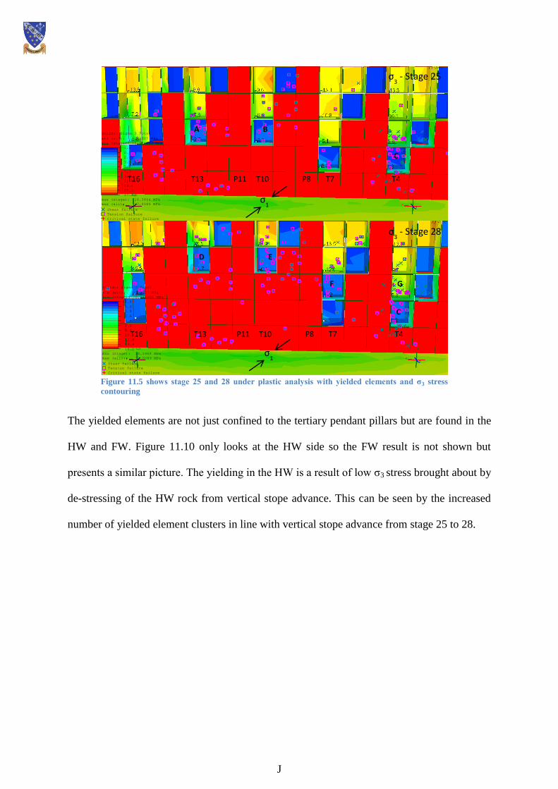
J
The yielded elements are not just confined to the tertiary pendant pillars but are found in the
HW and FW. Figure 11.10 only looks at the HW side so the FW result is not shown but
presents a similar picture. The yielding in the HW is a result of low σ3 stress brought about by
de-stressing of the HW rock from vertical stope advance. This can be seen by the increased
number of yielded element clusters in line with vertical stope advance from stage 25 to 28.
Solids: Sigma 3 Total
-1.8
0.0
1.8
3.6
5.4
7.2
9.0
10.8
12.6
14.4
16.2
min (all): -1.2207 MPa
min (stage): -0.983655 MPa
max (stage): 16.1468 MPa
max (all): 17.0089 MPa
Shear failure
Tension failure
Critical state failure
Solids: Sigma 3 Total
-1.8
0.1
2.0
3.9
5.8
7.7
9.6
11.5
13.4
15.3
17.2
min (all): -1.2207 MPa
min (stage): -0.926631 MPa
max (stage): 16.3864 MPa
max (all): 17.0089 MPa
Shear failure
Tension failure
Critical state failure
σ3 - Stage 25
σ3 - Stage 28
σ1
T16 T13 T10 T7 T4
T16 T13 T10 T7 T4
P8 P11
A B
C
D E
G F
C
P8 P11
σ1
Figure 11.5 shows stage 25 and 28 under plastic analysis with yielded elements and σ3 stress
contouring
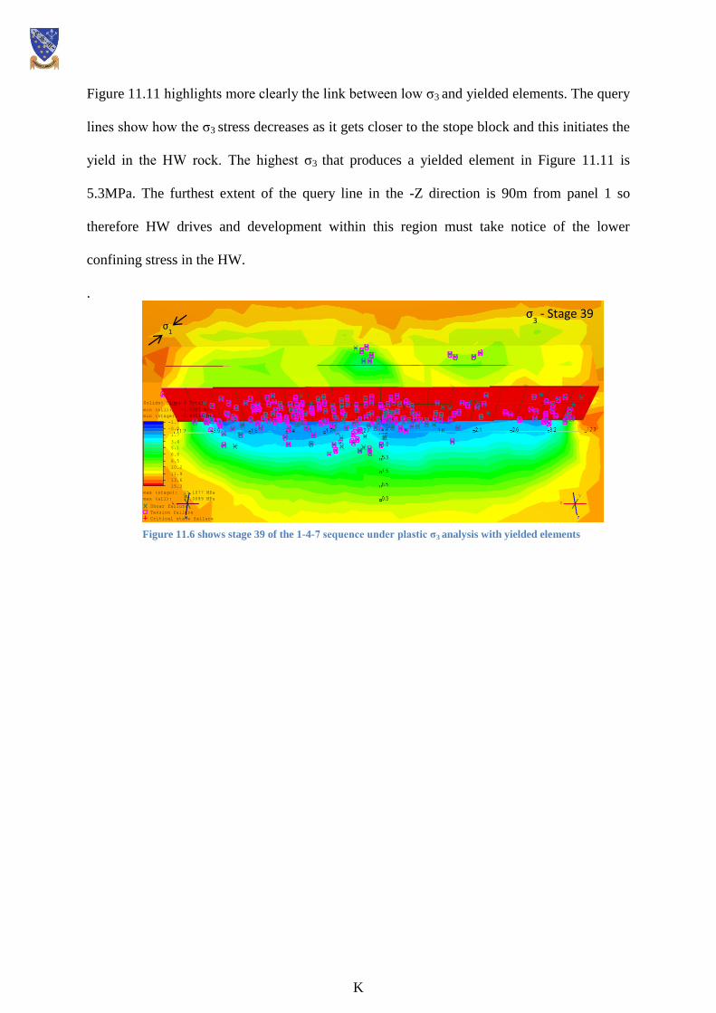
K
Figure 11.11 highlights more clearly the link between low σ3 and yielded elements. The query
lines show how the σ3 stress decreases as it gets closer to the stope block and this initiates the
yield in the HW rock. The highest σ3 that produces a yielded element in Figure 11.11 is
5.3MPa. The furthest extent of the query line in the -Z direction is 90m from panel 1 so
therefore HW drives and development within this region must take notice of the lower
confining stress in the HW.
.
Solids: Sigma 3 Total
-1.7
-0.0
1.7
3.4
5.1
6.8
8.5
10.2
11.9
13.6
15.3
min (all): -1.2207 MPa
min (stage): -0.94534 MPa
max (stage): 15.1077 MPa
max (all): 17.0089 MPa
Shear failure
Tension failure
Critical state failure
σ3 - Stage 39
σ1
Figure 11.6 shows stage 39 of the 1-4-7 sequence under plastic σ3 analysis with yielded elements
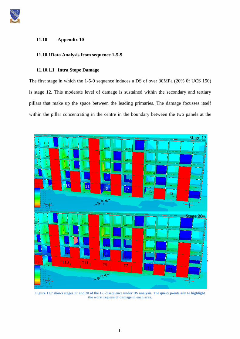
L
11.10 Appendix 10
11.10.1Data Analysis from sequence 1-5-9
11.10.1.1 Intra Stope Damage
The first stage in which the 1-5-9 sequence induces a DS of over 30MPa (20% 0f UCS 150)
is stage 12. This moderate level of damage is sustained within the secondary and tertiary
pillars that make up the space between the leading primaries. The damage focusses itself
within the pillar concentrating in the centre in the boundary between the two panels at the
Figure 11.7 shows stages 17 and 20 of the 1-5-9 sequence under DS analysis. The query points aim to highlight
the worst regions of damage in each area.
Solids: Deviatoric Stress
0.0
5.0
10.0
15.0
20.0
25.0
30.0
35.0
40.0
45.0
50.0
min (all): 0
min (stage): 0.00102299
max (stage): 38.7133
max (all): 49.5085
Solids: Deviatoric Stress
0.0
5.0
10.0
15.0
20.0
25.0
30.0
35.0
40.0
45.0
50.0
min (all): 0
min (stage): 0.00210887
max (stage): 39.7832
max (all): 49.5085
Stage 17
Stage 20
T13 T11 T9 T7 T5 T3
T13 T11 T9 T7 T5 T3
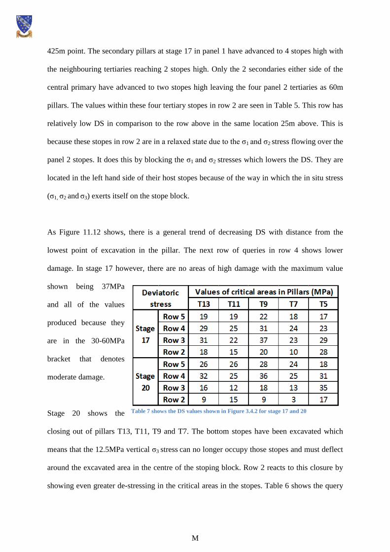
M
425m point. The secondary pillars at stage 17 in panel 1 have advanced to 4 stopes high with
the neighbouring tertiaries reaching 2 stopes high. Only the 2 secondaries either side of the
central primary have advanced to two stopes high leaving the four panel 2 tertiaries as 60m
pillars. The values within these four tertiary stopes in row 2 are seen in Table 5. This row has
relatively low DS in comparison to the row above in the same location 25m above. This is
because these stopes in row 2 are in a relaxed state due to the σ1 and σ2 stress flowing over the
panel 2 stopes. It does this by blocking the σ1 and σ2 stresses which lowers the DS. They are
located in the left hand side of their host stopes because of the way in which the in situ stress
(σ1, σ2 and σ3) exerts itself on the stope block.
As Figure 11.12 shows, there is a general trend of decreasing DS with distance from the
lowest point of excavation in the pillar. The next row of queries in row 4 shows lower
damage. In stage 17 however, there are no areas of high damage with the maximum value
shown being 37MPa
and all of the values
produced because they
are in the 30-60MPa
bracket that denotes
moderate damage.
Stage 20 shows the
closing out of pillars T13, T11, T9 and T7. The bottom stopes have been excavated which
means that the 12.5MPa vertical σ3 stress can no longer occupy those stopes and must deflect
around the excavated area in the centre of the stoping block. Row 2 reacts to this closure by
showing even greater de-stressing in the critical areas in the stopes. Table 6 shows the query
Table 7 shows the DS values shown in Figure 3.4.2 for stage 17 and 20
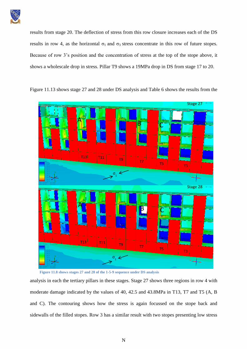
N
results from stage 20. The deflection of stress from this row closure increases each of the DS
results in row 4, as the horizontal σ1 and σ3 stress concentrate in this row of future stopes.
Because of row 3’s position and the concentration of stress at the top of the stope above, it
shows a wholescale drop in stress. Pillar T9 shows a 19MPa drop in DS from stage 17 to 20.
Figure 11.13 shows stage 27 and 28 under DS analysis and Table 6 shows the results from the
analysis in each the tertiary pillars in these stages. Stage 27 shows three regions in row 4 with
moderate damage indicated by the values of 40, 42.5 and 43.8MPa in T13, T7 and T5 (A, B
and C). The contouring shows how the stress is again focussed on the stope back and
sidewalls of the filled stopes. Row 3 has a similar result with two stopes presenting low stress
Figure 11.8 shows stages 27 and 28 of the 1-5-9 sequence under DS analysis
Stage 27
Stage 28
σ1
σ1
Solids: Deviatoric Stress
0.0
5.0
10.0
15.0
20.0
25.0
30.0
35.0
40.0
45.0
50.0
min (all): 0
min (stage): 0.00247067
max (stage): 45.7226
max (all): 49.5085
Solids: Deviatoric Stress
0.0
5.0
10.0
15.0
20.0
25.0
30.0
35.0
40.0
45.0
50.0
min (all): 0
min (stage): 0.000515451
max (stage): 46.1948
max (all): 49.5085
A B C
A B C
T13 T11 T9 T7 T5
T3
T13 T11 T9 T7 T5
T3
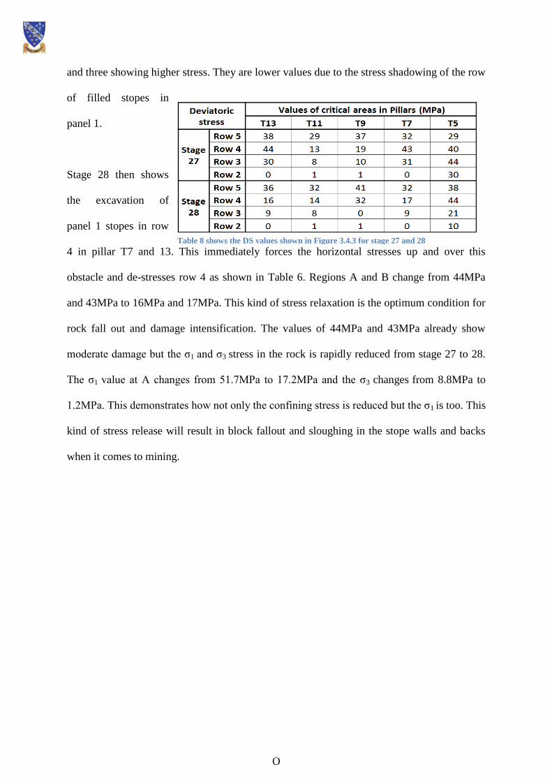
O
and three showing higher stress. They are lower values due to the stress shadowing of the row
of filled stopes in
panel 1.
Stage 28 then shows
the excavation of
panel 1 stopes in row
4 in pillar T7 and 13. This immediately forces the horizontal stresses up and over this
obstacle and de-stresses row 4 as shown in Table 6. Regions A and B change from 44MPa
and 43MPa to 16MPa and 17MPa. This kind of stress relaxation is the optimum condition for
rock fall out and damage intensification. The values of 44MPa and 43MPa already show
moderate damage but the σ1 and σ3 stress in the rock is rapidly reduced from stage 27 to 28.
The σ1 value at A changes from 51.7MPa to 17.2MPa and the σ3 changes from 8.8MPa to
1.2MPa. This demonstrates how not only the confining stress is reduced but the σ1 is too. This
kind of stress release will result in block fallout and sloughing in the stope walls and backs
when it comes to mining.
Table 8 shows the DS values shown in Figure 3.4.3 for stage 27 and 28

P
Figure 11.14 shows stage 30. The query points in row 2 are covered by the fill so therefore
can be assumed to be in a low stress environment. Row three queries are almost covered up
apart from pillar T5 and T15. This stage presents the highest recorded DS and therefore
highest definitive damage in the sequence with a value of 49.5MPa. This is sustained in row 4
of pillar T5 in the region labelled 47.8[MPa]. High figures are also found in pillar T15 in row
4 and pillars T7, T11 and T13 where the horizontal stress now has to deflect around 120m of
filled stopes as opposed to 30m, 60m or 90m in previous stages. This means that the
concentration of stresses becomes even more increased as well as increased stress shadowing
in the σ3 direction reducing confinement and increasing damage. As soon as this confinement
is released from the mining process it is highly likely that this release of confinement will
also induce block fallout from sidewalls or the stope back.
Table 9 shows the DS values shown in Figure 3.4.4 for stage 30
Figure 11.9 shows stage 30 of the 1-5-9 sequence under DS analysis.
Solids: Sigma 1 Total
-3.0
4.0
11.0
18.0
25.0
32.0
39.0
46.0
53.0
60.0
67.0
min (all): -0.0974957 MPa
min (stage): -0.0124845 MPa
max (stage): 57.2408 MPa
max (all): 59.867 MPa
σ1
Stage 30
T13 T11 T9
T7 T5
T15
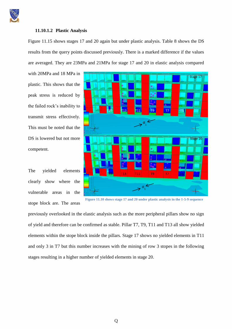
Q
11.10.1.2 Plastic Analysis
Figure 11.15 shows stages 17 and 20 again but under plastic analysis. Table 8 shows the DS
results from the query points discussed previously. There is a marked difference if the values
are averaged. They are 23MPa and 21MPa for stage 17 and 20 in elastic analysis compared
with 20MPa and 18 MPa in
plastic. This shows that the
peak stress is reduced by
the failed rock’s inability to
transmit stress effectively.
This must be noted that the
DS is lowered but not more
competent.
The yielded elements
clearly show where the
vulnerable areas in the
stope block are. The areas
previously overlooked in the elastic analysis such as the more peripheral pillars show no sign
of yield and therefore can be confirmed as stable. Pillar T7, T9, T11 and T13 all show yielded
elements within the stope block inside the pillars. Stage 17 shows no yielded elements in T11
and only 3 in T7 but this number increases with the mining of row 3 stopes in the following
stages resulting in a higher number of yielded elements in stage 20.
Figure 11.10 shows stage 17 and 20 under plastic analysis in the 1-5-9 sequence
Solids: Deviatoric Stress
0.0
5.0
10.0
15.0
20.0
25.0
30.0
35.0
40.0
45.0
50.0
min (all): 2.14064e-007
min (stage): 0.000917965
max (stage): 37.1948
max (all): 45.8538
Shear failure
Tension failure
Critical state failure
Solids: Deviatoric Stress
0.0
5.0
10.0
15.0
20.0
25.0
30.0
35.0
40.0
45.0
50.0
min (all): 2.14064e-007
min (stage): 0.00164431
max (stage): 33.9298
max (all): 45.8538
Shear failure
Tension failure
Critical state failure
σ1
σ1
Stage 17
Stage 20
T13 T11 T9 T7 T5
T13 T11 T9 T7 T5
T15
T15
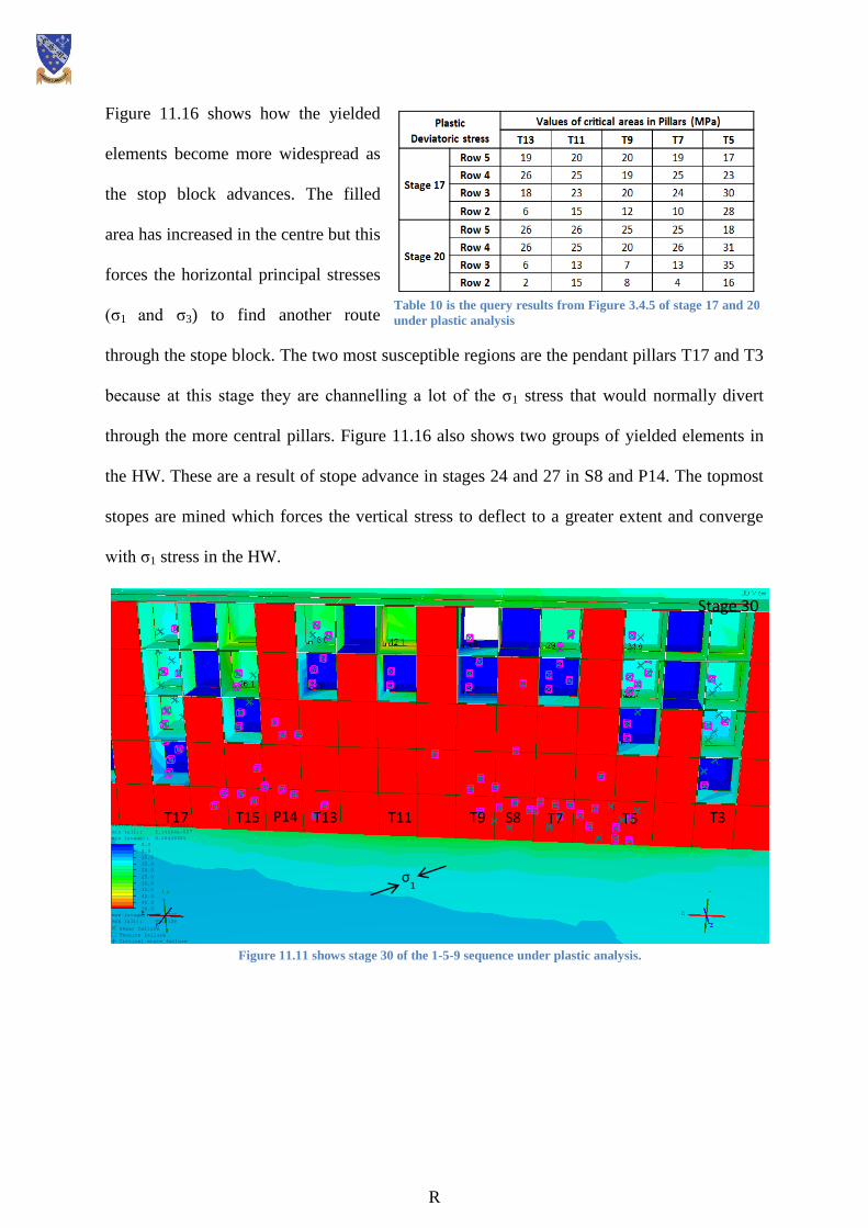
R
Figure 11.16 shows how the yielded
elements become more widespread as
the stop block advances. The filled
area has increased in the centre but this
forces the horizontal principal stresses
(σ1 and σ3) to find another route
through the stope block. The two most susceptible regions are the pendant pillars T17 and T3
because at this stage they are channelling a lot of the σ1 stress that would normally divert
through the more central pillars. Figure 11.16 also shows two groups of yielded elements in
the HW. These are a result of stope advance in stages 24 and 27 in S8 and P14. The topmost
stopes are mined which forces the vertical stress to deflect to a greater extent and converge
with σ1 stress in the HW.
Table 10 is the query results from Figure 3.4.5 of stage 17 and 20
under plastic analysis
Figure 11.11 shows stage 30 of the 1-5-9 sequence under plastic analysis.
Solids: Deviatoric Stress
0.0
5.0
10.0
15.0
20.0
25.0
30.0
35.0
40.0
45.0
50.0
min (all): 2.14064e-007
min (stage): 0.00448301
max (stage): 42.7747
max (all): 45.8538
Shear failure
Tension failure
Critical state failure
Stage 30
σ1
T13 T15 T11 T9 T7 T5 T3 T17 P14 S8
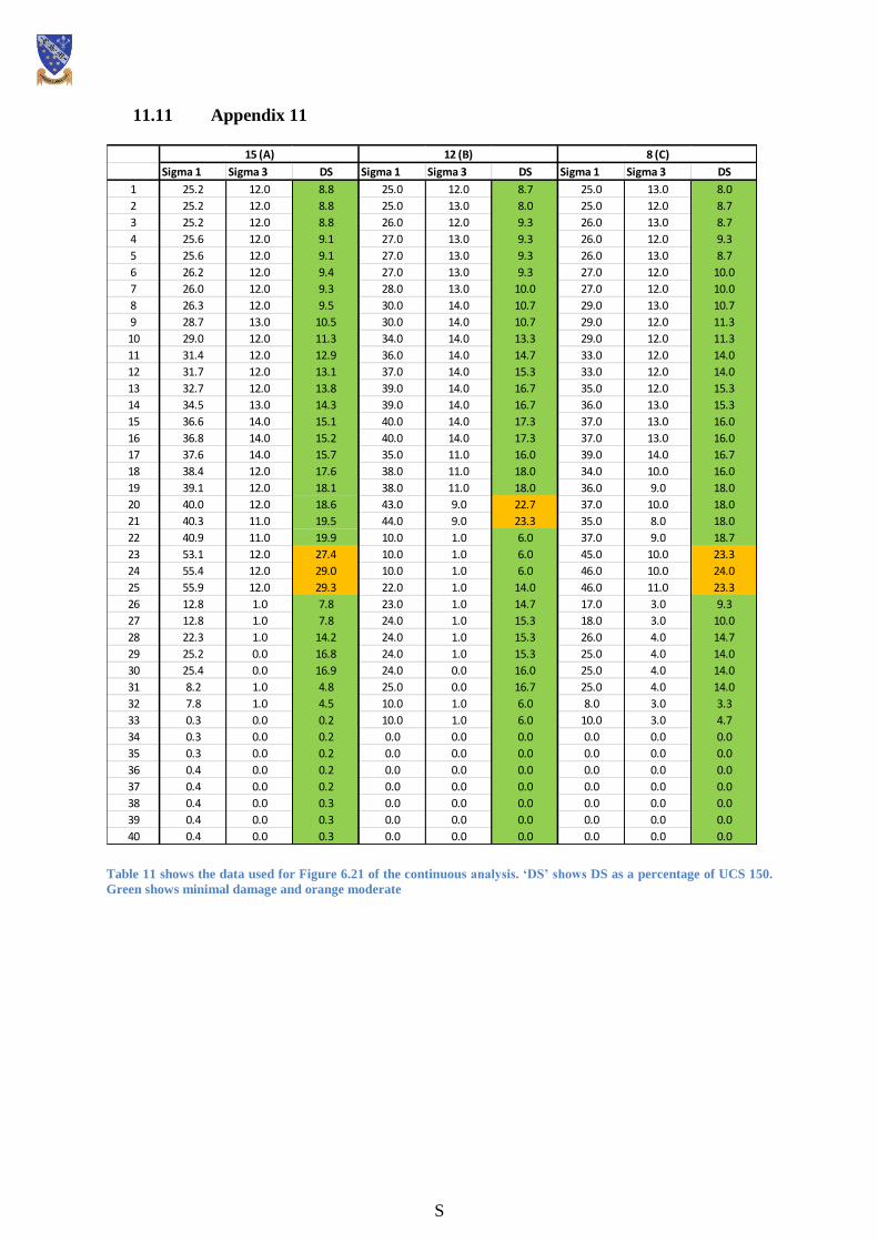
S
11.11 Appendix 11
Table 11 shows the data used for Figure 6.21 of the continuous analysis. ‘DS’ shows DS as a percentage of UCS 150.
Green shows minimal damage and orange moderate
Sigma 1 Sigma 3 DS Sigma 1 Sigma 3 DS Sigma 1 Sigma 3 DS
1 25.2 12.0 8.8 25.0 12.0 8.7 25.0 13.0 8.0
2 25.2 12.0 8.8 25.0 13.0 8.0 25.0 12.0 8.7
3 25.2 12.0 8.8 26.0 12.0 9.3 26.0 13.0 8.7
4 25.6 12.0 9.1 27.0 13.0 9.3 26.0 12.0 9.3
5 25.6 12.0 9.1 27.0 13.0 9.3 26.0 13.0 8.7
6 26.2 12.0 9.4 27.0 13.0 9.3 27.0 12.0 10.0
7 26.0 12.0 9.3 28.0 13.0 10.0 27.0 12.0 10.0
8 26.3 12.0 9.5 30.0 14.0 10.7 29.0 13.0 10.7
9 28.7 13.0 10.5 30.0 14.0 10.7 29.0 12.0 11.3
10 29.0 12.0 11.3 34.0 14.0 13.3 29.0 12.0 11.3
11 31.4 12.0 12.9 36.0 14.0 14.7 33.0 12.0 14.0
12 31.7 12.0 13.1 37.0 14.0 15.3 33.0 12.0 14.0
13 32.7 12.0 13.8 39.0 14.0 16.7 35.0 12.0 15.3
14 34.5 13.0 14.3 39.0 14.0 16.7 36.0 13.0 15.3
15 36.6 14.0 15.1 40.0 14.0 17.3 37.0 13.0 16.0
16 36.8 14.0 15.2 40.0 14.0 17.3 37.0 13.0 16.0
17 37.6 14.0 15.7 35.0 11.0 16.0 39.0 14.0 16.7
18 38.4 12.0 17.6 38.0 11.0 18.0 34.0 10.0 16.0
19 39.1 12.0 18.1 38.0 11.0 18.0 36.0 9.0 18.0
20 40.0 12.0 18.6 43.0 9.0 22.7 37.0 10.0 18.0
21 40.3 11.0 19.5 44.0 9.0 23.3 35.0 8.0 18.0
22 40.9 11.0 19.9 10.0 1.0 6.0 37.0 9.0 18.7
23 53.1 12.0 27.4 10.0 1.0 6.0 45.0 10.0 23.3
24 55.4 12.0 29.0 10.0 1.0 6.0 46.0 10.0 24.0
25 55.9 12.0 29.3 22.0 1.0 14.0 46.0 11.0 23.3
26 12.8 1.0 7.8 23.0 1.0 14.7 17.0 3.0 9.3
27 12.8 1.0 7.8 24.0 1.0 15.3 18.0 3.0 10.0
28 22.3 1.0 14.2 24.0 1.0 15.3 26.0 4.0 14.7
29 25.2 0.0 16.8 24.0 1.0 15.3 25.0 4.0 14.0
30 25.4 0.0 16.9 24.0 0.0 16.0 25.0 4.0 14.0
31 8.2 1.0 4.8 25.0 0.0 16.7 25.0 4.0 14.0
32 7.8 1.0 4.5 10.0 1.0 6.0 8.0 3.0 3.3
33 0.3 0.0 0.2 10.0 1.0 6.0 10.0 3.0 4.7
34 0.3 0.0 0.2 0.0 0.0 0.0 0.0 0.0 0.0
35 0.3 0.0 0.2 0.0 0.0 0.0 0.0 0.0 0.0
36 0.4 0.0 0.2 0.0 0.0 0.0 0.0 0.0 0.0
37 0.4 0.0 0.2 0.0 0.0 0.0 0.0 0.0 0.0
38 0.4 0.0 0.3 0.0 0.0 0.0 0.0 0.0 0.0
39 0.4 0.0 0.3 0.0 0.0 0.0 0.0 0.0 0.0
40 0.4 0.0 0.3 0.0 0.0 0.0 0.0 0.0 0.0
15 (A) 12 (B) 8 (C)
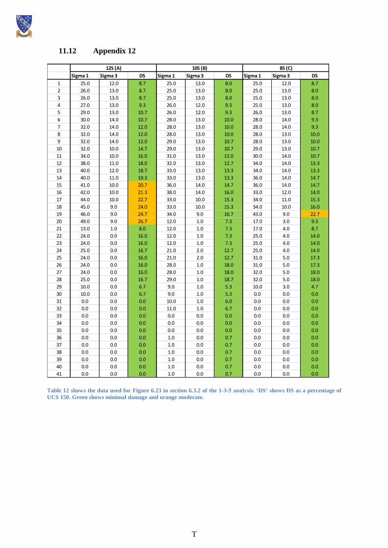
T
11.12 Appendix 12
Table 12 shows the data used for Figure 6.23 in section 6.3.2 of the 1-3-5 analysis. ‘DS’ shows DS as a percentage of
UCS 150. Green shows minimal damage and orange moderate.
Sigma 1 Sigma 3 DS Sigma 1 Sigma 3 DS Sigma 1 Sigma 3 DS
1 25.0 12.0 8.7 25.0 13.0 8.0 25.0 12.0 8.7
2 26.0 13.0 8.7 25.0 13.0 8.0 25.0 13.0 8.0
3 26.0 13.0 8.7 25.0 13.0 8.0 25.0 13.0 8.0
4 27.0 13.0 9.3 26.0 12.0 9.3 25.0 13.0 8.0
5 29.0 13.0 10.7 26.0 12.0 9.3 26.0 13.0 8.7
6 30.0 14.0 10.7 28.0 13.0 10.0 28.0 14.0 9.3
7 32.0 14.0 12.0 28.0 13.0 10.0 28.0 14.0 9.3
8 32.0 14.0 12.0 28.0 13.0 10.0 28.0 13.0 10.0
9 32.0 14.0 12.0 29.0 13.0 10.7 28.0 13.0 10.0
10 32.0 10.0 14.7 29.0 13.0 10.7 29.0 13.0 10.7
11 34.0 10.0 16.0 31.0 13.0 12.0 30.0 14.0 10.7
12 38.0 11.0 18.0 32.0 13.0 12.7 34.0 14.0 13.3
13 40.0 12.0 18.7 33.0 13.0 13.3 34.0 14.0 13.3
14 40.0 11.0 19.3 33.0 13.0 13.3 36.0 14.0 14.7
15 41.0 10.0 20.7 36.0 14.0 14.7 36.0 14.0 14.7
16 42.0 10.0 21.3 38.0 14.0 16.0 33.0 12.0 14.0
17 44.0 10.0 22.7 33.0 10.0 15.3 34.0 11.0 15.3
18 45.0 9.0 24.0 33.0 10.0 15.3 34.0 10.0 16.0
19 46.0 9.0 24.7 34.0 9.0 16.7 43.0 9.0 22.7
20 49.0 9.0 26.7 12.0 1.0 7.3 17.0 3.0 9.3
21 13.0 1.0 8.0 12.0 1.0 7.3 17.0 4.0 8.7
22 24.0 0.0 16.0 12.0 1.0 7.3 25.0 4.0 14.0
23 24.0 0.0 16.0 12.0 1.0 7.3 25.0 4.0 14.0
24 25.0 0.0 16.7 21.0 2.0 12.7 25.0 4.0 14.0
25 24.0 0.0 16.0 21.0 2.0 12.7 31.0 5.0 17.3
26 24.0 0.0 16.0 28.0 1.0 18.0 31.0 5.0 17.3
27 24.0 0.0 16.0 28.0 1.0 18.0 32.0 5.0 18.0
28 25.0 0.0 16.7 29.0 1.0 18.7 32.0 5.0 18.0
29 10.0 0.0 6.7 9.0 1.0 5.3 10.0 3.0 4.7
30 10.0 0.0 6.7 9.0 1.0 5.3 0.0 0.0 0.0
31 0.0 0.0 0.0 10.0 1.0 6.0 0.0 0.0 0.0
32 0.0 0.0 0.0 11.0 1.0 6.7 0.0 0.0 0.0
33 0.0 0.0 0.0 0.0 0.0 0.0 0.0 0.0 0.0
34 0.0 0.0 0.0 0.0 0.0 0.0 0.0 0.0 0.0
35 0.0 0.0 0.0 0.0 0.0 0.0 0.0 0.0 0.0
36 0.0 0.0 0.0 1.0 0.0 0.7 0.0 0.0 0.0
37 0.0 0.0 0.0 1.0 0.0 0.7 0.0 0.0 0.0
38 0.0 0.0 0.0 1.0 0.0 0.7 0.0 0.0 0.0
39 0.0 0.0 0.0 1.0 0.0 0.7 0.0 0.0 0.0
40 0.0 0.0 0.0 1.0 0.0 0.7 0.0 0.0 0.0
41 0.0 0.0 0.0 1.0 0.0 0.7 0.0 0.0 0.0
12S (A) 10S (B) 8S (C)
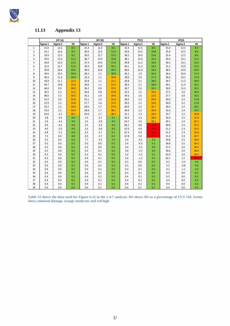
U
11.13 Appendix 13
Table 13 shows the data used for Figure 6.25 in the 1-4-7 analysis. DS shows DS as a percentage of UCS 150. Green
shows minimal damage, orange moderate and red high
Sigma 1 Sigma 3 DS Sigma 1 Sigma 3 DS Sigma 1 Sigma 3 DS Sigma 1 Sigma 3 DS
1 25.0 12.6 8.3 25.4 12.4 8.6 25.4 12.5 8.6 25.0 12.5 8.3
2 25.1 12.6 8.3 29.5 12.5 11.3 29.6 13.5 10.8 25.4 12.5 8.6
3 24.9 12.5 8.2 36.0 12.7 15.5 38.2 14.9 15.6 25.4 12.5 8.6
4 29.5 12.6 11.2 36.7 12.9 15.8 38.1 15.0 15.4 30.4 13.1 11.5
5 29.8 12.9 11.3 37.3 10.4 17.9 39.8 11.2 19.0 30.3 13.1 11.5
6 31.0 13.7 11.6 39.4 10.8 19.1 40.1 11.2 19.3 31.2 13.0 12.2
7 39.8 10.6 19.5 39.6 10.6 19.3 40.6 11.4 19.4 38.5 14.6 15.9
8 39.0 10.5 19.0 28.2 1.2 18.0 26.2 1.9 16.2 36.4 10.4 17.3
9 40.4 11.4 19.3 32.4 1.1 20.8 28.0 2.0 17.3 36.6 10.5 17.4
10 43.9 11.1 21.9 32.8 1.1 21.1 29.8 2.1 18.5 39.7 11.3 19.0
11 44.7 10.8 22.6 34.6 1.1 22.3 30.3 2.1 18.8 40.1 11.4 19.2
12 46.0 0.9 30.0 36.2 0.9 23.5 30.7 2.0 19.1 39.9 11.3 19.1
13 34.5 2.2 21.5 36.6 0.8 23.8 32.5 1.5 20.6 27.5 3.0 16.4
14 48.0 2.3 30.5 54.2 1.9 34.9 34.6 1.6 22.0 27.7 3.0 16.5
15 51.0 2.0 32.6 55.1 1.9 35.4 38.5 1.5 24.6 30.0 3.2 17.8
16 52.9 2.2 33.8 57.7 1.6 37.4 39.0 1.5 25.0 30.0 3.2 17.9
17 53.2 2.2 34.0 58.6 1.7 37.9 40.0 1.4 25.7 30.4 3.2 18.1
18 53.6 2.2 34.3 58.8 1.7 38.1 40.9 1.3 26.4 31.6 2.4 19.5
19 54.0 -3.2 38.1 59.0 1.7 38.2 41.1 1.3 26.5 33.7 2.5 20.8
20 3.8 -3.4 4.8 3.4 -2.7 4.1 43.4 1.4 28.0 34.0 2.5 21.0
21 3.9 -3.4 4.9 3.5 -2.9 4.2 63.7 5.0 39.1 40.1 2.4 25.1
22 4.0 -3.5 4.9 3.5 -2.9 4.2 66.1 4.8 40.9 40.8 2.5 25.5
23 4.0 -2.0 4.0 3.5 -3.0 4.3 67.0 4.9 41.4 51.2 2.3 32.6
24 6.8 -2.2 6.0 6.5 -2.7 6.1 67.3 4.9 41.6 51.2 2.3 32.6
25 7.2 0.0 4.8 6.5 -2.7 6.2 67.8 5.0 41.9 51.4 2.3 32.7
26 0.3 0.0 0.2 7.7 -3.5 7.5 3.4 -4.2 5.0 54.8 2.5 34.9
27 0.3 0.0 0.2 0.3 0.0 0.2 3.4 -4.3 5.1 56.8 2.5 36.2
28 0.3 0.0 0.2 0.3 0.0 0.2 3.0 -1.5 3.0 57.3 2.6 36.5
29 0.3 0.0 0.2 0.3 0.1 0.2 3.0 -1.5 3.0 59.6 2.0 38.4
30 0.3 0.0 0.2 0.3 0.1 0.2 3.2 -1.5 3.1 61.0 2.0 39.3
31 0.3 0.0 0.2 0.4 0.1 0.2 3.6 -1.2 3.2 63.1 2.2 40.6
32 0.3 0.0 0.2 0.4 0.1 0.2 0.3 0.0 0.2 4.2 -3.3 5.0
33 0.4 0.0 0.2 0.4 0.1 0.2 0.3 0.0 0.2 5.2 -0.8 4.0
34 0.4 0.0 0.2 0.4 0.1 0.2 0.3 0.1 0.2 4.2 -1.1 3.5
35 0.4 0.0 0.2 0.4 0.1 0.2 0.3 0.1 0.2 0.3 0.0 0.2
36 0.4 0.0 0.2 0.4 0.1 0.2 0.4 0.1 0.2 0.3 0.0 0.2
37 0.4 0.0 0.2 0.4 0.1 0.2 0.4 0.1 0.2 0.4 0.0 0.2
38 0.4 0.0 0.2 0.4 0.1 0.2 0.4 0.1 0.2 0.4 0.0 0.2
39 0.4 0.0 0.2 0.4 0.1 0.2 0.4 0.1 0.2 0.4 0.0 0.2
13T (A) 10T (B) 7T(C) 4T(D)
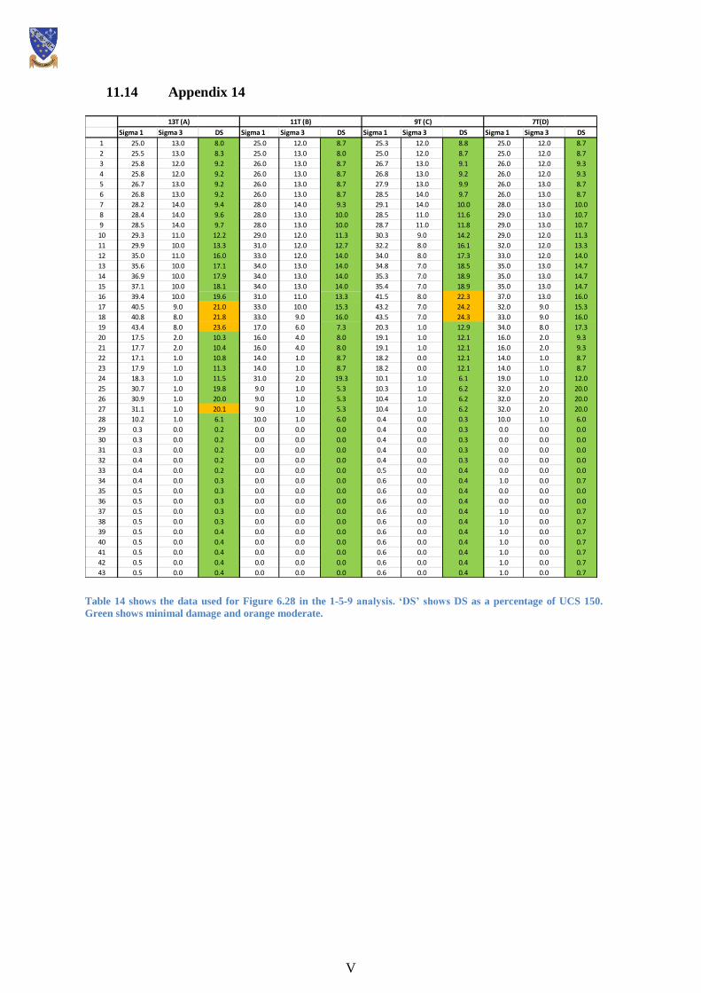
V
11.14 Appendix 14
Table 14 shows the data used for Figure 6.28 in the 1-5-9 analysis. ‘DS’ shows DS as a percentage of UCS 150.
Green shows minimal damage and orange moderate.
Sigma 1 Sigma 3 DS Sigma 1 Sigma 3 DS Sigma 1 Sigma 3 DS Sigma 1 Sigma 3 DS
1 25.0 13.0 8.0 25.0 12.0 8.7 25.3 12.0 8.8 25.0 12.0 8.7
2 25.5 13.0 8.3 25.0 13.0 8.0 25.0 12.0 8.7 25.0 12.0 8.7
3 25.8 12.0 9.2 26.0 13.0 8.7 26.7 13.0 9.1 26.0 12.0 9.3
4 25.8 12.0 9.2 26.0 13.0 8.7 26.8 13.0 9.2 26.0 12.0 9.3
5 26.7 13.0 9.2 26.0 13.0 8.7 27.9 13.0 9.9 26.0 13.0 8.7
6 26.8 13.0 9.2 26.0 13.0 8.7 28.5 14.0 9.7 26.0 13.0 8.7
7 28.2 14.0 9.4 28.0 14.0 9.3 29.1 14.0 10.0 28.0 13.0 10.0
8 28.4 14.0 9.6 28.0 13.0 10.0 28.5 11.0 11.6 29.0 13.0 10.7
9 28.5 14.0 9.7 28.0 13.0 10.0 28.7 11.0 11.8 29.0 13.0 10.7
10 29.3 11.0 12.2 29.0 12.0 11.3 30.3 9.0 14.2 29.0 12.0 11.3
11 29.9 10.0 13.3 31.0 12.0 12.7 32.2 8.0 16.1 32.0 12.0 13.3
12 35.0 11.0 16.0 33.0 12.0 14.0 34.0 8.0 17.3 33.0 12.0 14.0
13 35.6 10.0 17.1 34.0 13.0 14.0 34.8 7.0 18.5 35.0 13.0 14.7
14 36.9 10.0 17.9 34.0 13.0 14.0 35.3 7.0 18.9 35.0 13.0 14.7
15 37.1 10.0 18.1 34.0 13.0 14.0 35.4 7.0 18.9 35.0 13.0 14.7
16 39.4 10.0 19.6 31.0 11.0 13.3 41.5 8.0 22.3 37.0 13.0 16.0
17 40.5 9.0 21.0 33.0 10.0 15.3 43.2 7.0 24.2 32.0 9.0 15.3
18 40.8 8.0 21.8 33.0 9.0 16.0 43.5 7.0 24.3 33.0 9.0 16.0
19 43.4 8.0 23.6 17.0 6.0 7.3 20.3 1.0 12.9 34.0 8.0 17.3
20 17.5 2.0 10.3 16.0 4.0 8.0 19.1 1.0 12.1 16.0 2.0 9.3
21 17.7 2.0 10.4 16.0 4.0 8.0 19.1 1.0 12.1 16.0 2.0 9.3
22 17.1 1.0 10.8 14.0 1.0 8.7 18.2 0.0 12.1 14.0 1.0 8.7
23 17.9 1.0 11.3 14.0 1.0 8.7 18.2 0.0 12.1 14.0 1.0 8.7
24 18.3 1.0 11.5 31.0 2.0 19.3 10.1 1.0 6.1 19.0 1.0 12.0
25 30.7 1.0 19.8 9.0 1.0 5.3 10.3 1.0 6.2 32.0 2.0 20.0
26 30.9 1.0 20.0 9.0 1.0 5.3 10.4 1.0 6.2 32.0 2.0 20.0
27 31.1 1.0 20.1 9.0 1.0 5.3 10.4 1.0 6.2 32.0 2.0 20.0
28 10.2 1.0 6.1 10.0 1.0 6.0 0.4 0.0 0.3 10.0 1.0 6.0
29 0.3 0.0 0.2 0.0 0.0 0.0 0.4 0.0 0.3 0.0 0.0 0.0
30 0.3 0.0 0.2 0.0 0.0 0.0 0.4 0.0 0.3 0.0 0.0 0.0
31 0.3 0.0 0.2 0.0 0.0 0.0 0.4 0.0 0.3 0.0 0.0 0.0
32 0.4 0.0 0.2 0.0 0.0 0.0 0.4 0.0 0.3 0.0 0.0 0.0
33 0.4 0.0 0.2 0.0 0.0 0.0 0.5 0.0 0.4 0.0 0.0 0.0
34 0.4 0.0 0.3 0.0 0.0 0.0 0.6 0.0 0.4 1.0 0.0 0.7
35 0.5 0.0 0.3 0.0 0.0 0.0 0.6 0.0 0.4 0.0 0.0 0.0
36 0.5 0.0 0.3 0.0 0.0 0.0 0.6 0.0 0.4 0.0 0.0 0.0
37 0.5 0.0 0.3 0.0 0.0 0.0 0.6 0.0 0.4 1.0 0.0 0.7
38 0.5 0.0 0.3 0.0 0.0 0.0 0.6 0.0 0.4 1.0 0.0 0.7
39 0.5 0.0 0.4 0.0 0.0 0.0 0.6 0.0 0.4 1.0 0.0 0.7
40 0.5 0.0 0.4 0.0 0.0 0.0 0.6 0.0 0.4 1.0 0.0 0.7
41 0.5 0.0 0.4 0.0 0.0 0.0 0.6 0.0 0.4 1.0 0.0 0.7
42 0.5 0.0 0.4 0.0 0.0 0.0 0.6 0.0 0.4 1.0 0.0 0.7
43 0.5 0.0 0.4 0.0 0.0 0.0 0.6 0.0 0.4 1.0 0.0 0.7
13T (A) 11T (B) 9T (C) 7T(D)