Embed Size (px)
Citation preview
Western Australian School of Mines
Stope Boundary Optimisation in Underground Mining Based on a
Heuristic Approach
Don Suneth Sameera Sandanayake
This thesis is presented for the Degree of
Doctor of Philosophy
of
Curtin University
August 2014

i
In loving memory of my grandmother, Wasantha Sandanayake (1917-2000)

ii
To the best of my knowledge and belief this thesis contains no material
previously published by any other person except where due
acknowledgment has been made. This thesis contains no material which has
been accepted for the award of any other degree or diploma in any
university.
iii
PUBLICATIONS INCORPORATED INTO THIS
THESIS
Sandanayake, D.S.S., 2013. Stope boundary optimisation in underground mining
based on a heuristic approach. Akita University Leading Program 2013 workshop
delivered at Akita University, Japan, 25 September 2013.
Sandanayake, D.S.S., Topal, E., Asad, M.W.A., 2014. Implementing a New
Heuristic Approach to Underground Mine Stope Layout Problem, paper will be
presented to Ore Body Modelling and Strategic Mine Planning 2014 Symposium,
Perth, Australia, 24-26 November 2014 (Accepted).
Sandanayake, D.S.S., Topal, E., Asad, M.W.A., 2014. A heuristic approach to
optimal design of an underground mine stope layout, Applied Soft Computing (under
review).
Sandanayake, D.S.S., Topal, E., Asad, M.W.A., 2014. Designing an optimal stope
layout for underground mining based on a heuristic algorithm, International Journal
of Mining, Reclamation and Environment (under review).
iv
ACKNOWLEDGEMENTS
I would like to express my gratitude to the following people for their assistance in the
completion of my PhD studies at WA School of Mines, Curtin University:
My supervisor Professor Erkan Topal, for his fundamental role in guiding me
throughout my research period at WA School of Mines, Curtin University.
My co-supervisor Dr. Mohammad Waqar Ali Asad, for his valuable
suggestions and assistance in improving the manuscript of this thesis.
Dr. Mahnida Kuruppu, for coordinating my enrolment in the PhD degree
programme at WA School of Mines, Curtin University.
The academic staff of WA School of Mines, who have always been very
supportive in both academic and non-academic matters.
My colleagues, Mr. Yu Li, Mr. Hyong Doo Jang, Ms. Ayako Kusui, Mr.
Zhao Fu, Mr. Ushan De Zoysa, Mr. Zela Tanlega, Mrs. Ndisha Mbedzi, Mr.
Mohammad Moridi and Mr. Mai Luan, for their encouragement during my
studies.
Mr. Jovan Hamovic and Mr Steph Cantin of Dassault Systèmes GEOVIA
Ltd. for their assistance in GEOVIA Surpac™ software visualisations.
Dr. Mehmet Cigla of MineSight Applications Ltd. for his assistance in the
validation study of the project.
My dear parents whose role in my life is immense.
I dedicate this thesis to the loving memory of my grandmother Wasantha
Sandanayake who always admired and supported my academic journey.
v
ABSTRACT
A stope can be defined as an underground production zone where ore is extracted
from the surrounding rock mass using underground mining methods. Employing the
optimal layout of stopes maximises the discounted value of future cash flows subject
to inherent physical, geotechnical and geological constraints over the life span of
underground mining operations. Therefore, stope optimisation is a key requirement
over the duration of an underground mining venture. Numerous approaches have
been introduced to address the stope layout optimisation problem. Considering the
computational complexity and size of the problem, none of these approaches
guarantee true optimality in three-dimensional (3D) space. Thus, the research focus
of this PhD thesis is the development of an innovative heuristic algorithm to generate
a near-optimal stope layout for a given resource model. Due to the non-deterministic
polynomial-time hard (NP-hard) combinatorial nature of the problem, a new heuristic
algorithm is proposed to solve the stope optimisation problem. The proposed
algorithm takes a 3D resource model as its input, generates a set of possible solutions
and selects the solution with the maximum cash flow subject to associated costs of
extraction as the optimum solution to a given resource model. Improvements to the
algorithm increased the performance by applying multi-threading concepts from
object-oriented programming. Case studies (referenced by A to G in the alphabetical
order) are presented to demonstrate the applicability of the algorithm based on a
resource model that represents a copper deposit in different mining scenarios.
Among these defined cases, case D with a variable stopes size of 3 3 3 3
3 4 generated the most profitable solution. Further changes to the input
configuration improved the solution values of cases A and D by 3.8%. Validation
studies show that the proposed algorithm generates more profitable solutions than
two existing algorithms: the maximum value neighbourhood (MVN) algorithm and
the Sens and Topal heuristic approach. In comparison to the MVN algorithm, the
proposed algorithm generated 11.2% and 22.5% superior solutions for cases B and
G. In comparison to the Sens and Topal heuristic approach, the proposed algorithm
generated 7.3% and 5.6% superior solutions for cases A and D.
vi
TABLE OF CONTENTS
Publications incorporated into this thesis .................................................................... iii
Acknowledgements ..................................................................................................... iv
Abstract ........................................................................................................................ v
Table of contents ......................................................................................................... vi
List of figures .............................................................................................................. ix
List of tables ................................................................................................................ xi
CHAPTER 1 Introduction ........................................................................................ 1
1.1 Problem statement ......................................................................................... 1
1.2 Objectives ...................................................................................................... 4
1.3 Scope ............................................................................................................. 5
1.4 Methodology ................................................................................................. 5
1.5 Significance and relevance ............................................................................ 5
1.6 Thesis overview ............................................................................................. 6
CHAPTER 2 Underground stope optimisation ........................................................ 8
2.1 Fundamentals of stoping methods ................................................................. 9
2.1.1 Naturally supported stoping methods................................................... 10
2.1.2 Artificially supported stoping methods ................................................ 11
2.2 The existing stope optimisation algorithms ................................................. 11
2.2.1 Dynamic programming solution for stope optimisation ...................... 12
2.2.2 Octree division algorithm ..................................................................... 12
2.2.3 Branch and bound algorithm ................................................................ 13
2.2.4 Floating stope algorithm ...................................................................... 14
2.2.5 Multiple pass floating stope process .................................................... 15
2.2.6 Maximum Value Neighbourhood algorithm ........................................ 16
2.2.7 Mixed Integer Programming-based algorithm ..................................... 18
2.2.8 Sens and Topal heuristic approach ....................................................... 18
vii
2.2.9 Network flow method .......................................................................... 19
2.3 Use of heuristics for combinatorial optimisation ........................................ 20
2.3.1 Types of heuristic algorithms ............................................................... 21
2.4 Summary ..................................................................................................... 22
CHAPTER 3 Development of the proposed algorithm .......................................... 23
3.1 Block regularisation .................................................................................... 23
3.2 Converting the geological model into an economic model ......................... 26
3.3 Stope generation .......................................................................................... 26
3.3.1 Stope generation algorithm .................................................................. 29
3.3.2 Extracting positive economic stopes .................................................... 33
3.4 Generating the optimum solution ................................................................ 34
3.4.1 Definition of the non-overlapping stope constraint ............................. 35
3.4.2 Definition of the unique set constraint ................................................. 36
3.4.3 Steps of the algorithm .......................................................................... 36
3.5 Handling mining scenarios .......................................................................... 38
3.5.1 Application of variable stope sizes ...................................................... 38
3.5.2 Provision of mining levels ................................................................... 42
3.5.3 Provision of pillars ............................................................................... 44
3.5.4 Stope shaper: post-optimum improvements to the solution ................. 45
3.6 Performance improvements and limitations ................................................ 47
3.6.1 Stope generation performance.............................................................. 47
3.6.2 Stope optimisation performance .......................................................... 49
3.6.3 Limitation of the optimum solutions generated ................................... 50
CHAPTER 4 Implementation of the proposed algorithm ...................................... 52
4.1 Block regularisation for cases a to f ............................................................ 52
4.2 Converting the geological model into an economic model for cases a to f . 53
4.3 Cases based on different mining scenarios .................................................. 53
viii
4.3.1 Summary of outcomes for cases a to f ................................................. 55
4.4 Application of parallel multi-threading ....................................................... 56
4.5 Applying the stope shaper ........................................................................... 59
4.6 Improvements to the solution based on structural changes in the input ...... 60
4.6.1 3D orientation of the stope structure .................................................... 61
4.6.2 Percentage of positive stopes based on economic value ...................... 62
4.6.3 Combination of the optimum 3D orientation and input percentage ..... 64
4.7 Validation of the proposed algorithm .......................................................... 65
4.7.1 Comparison with the Sens and Topal heuristic approach .................... 65
4.7.2 Comparison with the MVN algorithm ................................................. 67
4.8 Application interface ................................................................................... 69
CHAPTER 5 Conclusions and recommendations .................................................. 70
5.1 Thesis summary ........................................................................................... 70
5.2 Recommendations ....................................................................................... 72
References .................................................................................................................. 74
Appendix A ................................................................................................................ 79
1. Data set up process ............................................................................................. 79
2. Implementation ................................................................................................... 81
2.1 Setting the SQL and block model unit parameters ....................................... 82
2.2 Regulariser .................................................................................................... 83
2.3 Economic value calculator ............................................................................ 84
2.4 Stope generator ............................................................................................. 84
2.5 Stope optimiser ............................................................................................. 86
2.5.1 Selecting the spatial order of stopes ...................................................... 87
2.5.2 Selecting the percentage of stopes ........................................................ 87
2.5.3 Implementation of the stope optimiser .................................................. 88
2.6 Quick solver .................................................................................................. 88
ix
2.7 Stope shaper and extraction of ore blocks .................................................... 89
2.8 Progress reporter ........................................................................................... 89
Appendix B ................................................................................................................ 90
1. Converting the geological model into an economic model ................................ 90
2. Creating a unique identifier to facilitate stope generation .................................. 91
3. Generating stopes ............................................................................................... 92
4. Extracting a list of positive stopes ...................................................................... 94
LIST OF FIGURES
Figure 1.1 (a) Three possible stopes (b) Border of the candidate pool of blocks for
stope creation. .............................................................................................................. 2
Figure 1.2 Representative layout of a stope in an underground mine. ........................ 3
Figure 2.1 Two-dimensional view of an open pit mining geometry. .......................... 9
Figure 2.2 A close-up of production operations with a stope of an underground mine
(Gertch and Bullock, 1998). ....................................................................................... 10
Figure 2.3 (a) Octree division. (b) Successive removal of sub-volumes (Cheimanoff
et al., 1989). ................................................................................................................ 13
Figure 2.4 Row of economic value blocks. ............................................................... 13
Figure 2.5 Cumulative function for the row of economic blocks. ............................ 14
Figure 2.6 The overlapping problem with the floating stope algorithm. .................. 15
Figure 2.7 Example illustrating the main problem with the MVN algorithm. .......... 17
Figure 2.8 The problem with Sens and Topal heuristic approach............................. 19
Figure 2.9 (a) Block model constructed using the cylindrical coordinate system. (b)
Typical arcs with vertical links of precedence (Bai et al., 2013). .............................. 20
Figure 3.1 General flow of the algorithm.................................................................. 23
Figure 3.2 Example illustrating the block regularisation process. ............................ 24
Figure 3.3 Block model with a stope size of 2 3 2 blocks and a block size of 5 5
5 m. .......................................................................................................................... 27
Figure 3.4 Stope generation process. ........................................................................ 27
Figure 3.5 Mining block and stope notations. ........................................................... 28
Figure 3.6 Block identifier for a two-dimensional example. .................................... 29
x
Figure 3.7 The stope that begins at the block identifier (2,3) and ends at the block
identifier (3,4). ........................................................................................................... 31
Figure 3.8 Steps of the stope generation algorithm................................................... 32
Figure 3.9 Generation of nine possible stopes for a two-dimensional example. ...... 33
Figure 3.10 Algorithmic flow required to generate the optimum solution. .............. 37
Figure 3.11 Steps of the stope size variation algorithm. ........................................... 39
Figure 3.12 Generating variable stope sizes. ............................................................ 41
Figure 3.13 Generating stopes on a level by level basis compared with a block by
block basis along the z axis. ....................................................................................... 42
Figure 3.14 Stope generating algorithm with incorporation of levels. ..................... 43
Figure 3.15 Notations for pillar separation. .............................................................. 44
Figure 3.16 Optimum stope layout for a given level on the x,y plane. ..................... 45
Figure 3.17 Layout of the modified stope boundary for the example. ...................... 46
Figure 3.18 EQATEC profile showing method details of the original stope
generation algorithm. ................................................................................................. 47
Figure 3.19 EQATEC profile showing the method calls and details for the modified
stope generation algorithm. ........................................................................................ 49
Figure 3.20 Incorporation of parallel threading into step (iii) of the algorithm. ....... 50
Figure 3.21 Steps of the modified stope optimisation algorithm. ............................. 51
Figure 4.1 Grade distribution of the copper deposit. ................................................ 52
Figure 4.2 The regularised economic block model. .................................................. 53
Figure 4.3 Convergence of the solution value for Cases A-F .................................... 55
Figure 4.4 Three-dimensional view of the optimal stope layouts in Cases A-F. ....... 56
Figure 4.5 Solution times for Cases A-F prior to the implementation of multi-
threading. .................................................................................................................... 57
Figure 4.6 Performance comparison between the original and modified algorithms
for Case A. ................................................................................................................. 57
Figure 4.7 Performance comparison between the original and modified algorithms
for Case B. .................................................................................................................. 58
Figure 4.8 Performance comparison between the original and modified algorithms
for Case C. .................................................................................................................. 58
Figure 4.9 Performance comparison between the original and modified algorithms
for Case D. ................................................................................................................. 58
xi
Figure 4.10 Performance comparison between the original and modified algorithms
for Case E. .................................................................................................................. 59
Figure 4.11 Performance comparison between the original and modified algorithms
for Case F. .................................................................................................................. 59
Figure 4.12 (a) Boundary and enclosed stopes, (b) enclosed stopes and boundary ore
blocks. ........................................................................................................................ 60
Figure 4.13 Superimposition of the ore blocks in the resource model...................... 60
Figure 4.14 Results obtained after variation in the input based on the percentage of
stopes for Cases A and D. .......................................................................................... 63
Figure 4.15 Visualisations of the optimum solutions to Case A using (a) the
proposed algorithm and (b) the Sens and Topal approach. ........................................ 65
Figure 4.16 Visualisations of the optimum solutions to Case D using (a) the
proposed algorithm and (b) the Sens and Topal approach. ........................................ 66
Figure 4.17 Visualisations of the mining blocks to Case B using (a) the proposed
algorithm and (b) the MVN algorithm. ...................................................................... 67
Figure 4.18 Visualisations of the mining blocks to Case G using (a) the proposed
algorithm and (b) the MVN algorithm. ...................................................................... 68
Figure 4.19 User interface for the stope optimisation algorithm. ............................. 69
LIST OF TABLES
Table 3.1 Summary of the stopes generated for the example. ................................... 34
Table 3.2 Overlapping scenarios for two stopes. ....................................................... 35
Table 3.3 Stope size creation for Example 1.............................................................. 40
Table 3.4 Stope size creation for Example 2.............................................................. 40
Table 3.5 Stope size creation for Example 3.............................................................. 41
Table 4.1 Details of the original block model. ........................................................... 52
Table 4.2 Details of the regularised block model. ..................................................... 53
Table 4.3 Summary of the stopes generated for the cases. ........................................ 54
Table 4.4 Values of the parameters for the optimal solution to Cases A-F. .............. 55
Table 4.5 Summary of the optimum solutions for six stope orientations. ................. 61
Table 4.6 Comparison of solutions obtained using x,y,z and y,x,z orientations for
Cases A and D. ........................................................................................................... 62
xii
Table 4.7 Summary of the optimum solutions for Cases A and D based on the
percentage of stopes. .................................................................................................. 63
Table 4.8 Summary of the optimum solutions obtained based on 60–100% stopes
after 500 iterations...................................................................................................... 64
Table 4.9 Summary of the optimum solutions for Case A based on the combined
input parameters. ........................................................................................................ 65
Table 4.10 Comparison of solutions obtained using proposed algorithm and Sens and
Topal approach. .......................................................................................................... 66
Table 4.11 Comparison of solutions obtained using the proposed algorithm and the
MVN algorithm for Case B. ....................................................................................... 68
1
Stope Boundary Optimisation in Underground Mining Based on a Heuristic Approach
CHAPTER 1 INTRODUCTION
Stope optimisation plays a pivotal role in the planning stages of underground mining
projects, because the optimal stope design impacts the value of the project revenue or
the discounted value of the future cash flows. In addition, the guidance of mining
operations given the best stope design is of paramount importance as it ensures the
best utilisation and management of the human and financial resources involved in an
underground mining project. Few algorithms have been developed to optimise the
stope boundary, and none guarantee true optimality in a three-dimensional (3D)
space. Thus, an efficient algorithm needs further development by mine planning
engineers to optimise stope layouts while satisfying physical mining constraints and
maximising the profit from operations.
1.1 PROBLEM STATEMENT
The demand for mineral commodities has been increasing rapidly due to global
industrial and population growth with limited resources and depletion of shallow,
easily accessible deposits. As a consequence, the mining industry has been
compelled to explore deeper deposits and extract minerals using underground mining
methods to meet increasing market demands. To maintain a healthy balance between
market demand and mine production rates, underground mine planning and design
tools need to be optimised in a manner that facilitates the maximum recovery of a
resource and minimum extraction costs (Kumral, 2004; Little et al., 2011).
Therefore, it is essential that mine planners employ high quality underground
optimisation tools that can guarantee the generation of the optimum design solutions
for mining-related problems.
Over the years, underground mine planning has advanced into three major areas:
stope boundary and layout definition; development and infrastructure placement; and
production scheduling (Sens & Topal, 2009). Of these three areas, stope boundary
optimisation is particularly significant for underground mining projects because the
optimal stope design ensures optimal production rates of ore with minimum amount
of waste, and it guides production scheduling over the life-term of the mine.
However, developing techniques for stope optimisation is a complex task because it
2
Stope Boundary Optimisation in Underground Mining Based on a Heuristic Approach
requires the satisfaction of a multitude of mining constraints while maximising the
overall profit.
Underground deposits are modelled using exploration data with geostatistical
techniques in order to facilitate the selection of stoping methods and stoping
dimensions (Asad et al., 2013; Kumral, 2013; Topal, 2008). These models are
collections of 3D blocks that represent shapes, volumes, tonnages and grades of
solids, which comprise ore zones, waste zones and other zones of geological interest.
The models used are small-scale representations of ore deposits and their
surroundings. Ore is accompanied by waste material, thus it is a difficult task to
identify economic collections of production zones and satisfy objectives of
maximising productivity in mining operations (Asad, 2011; Hustrulid, 2006).
The number of blocks that can be included in a stope depend on other factors such as
geotechnical constraints and the sizes of the machines utilised (Alford et al., 2007;
Ataee-pour, 2004). Two or more profitable stopes may share a few blocks in some
cases, and decisions have to be made to select the most profitable stopes, because
overlapping stopes cannot be physically mined together. In general, these
requirements dictate the minimum and maximum stope dimensions, final stope
layout and mining operations.
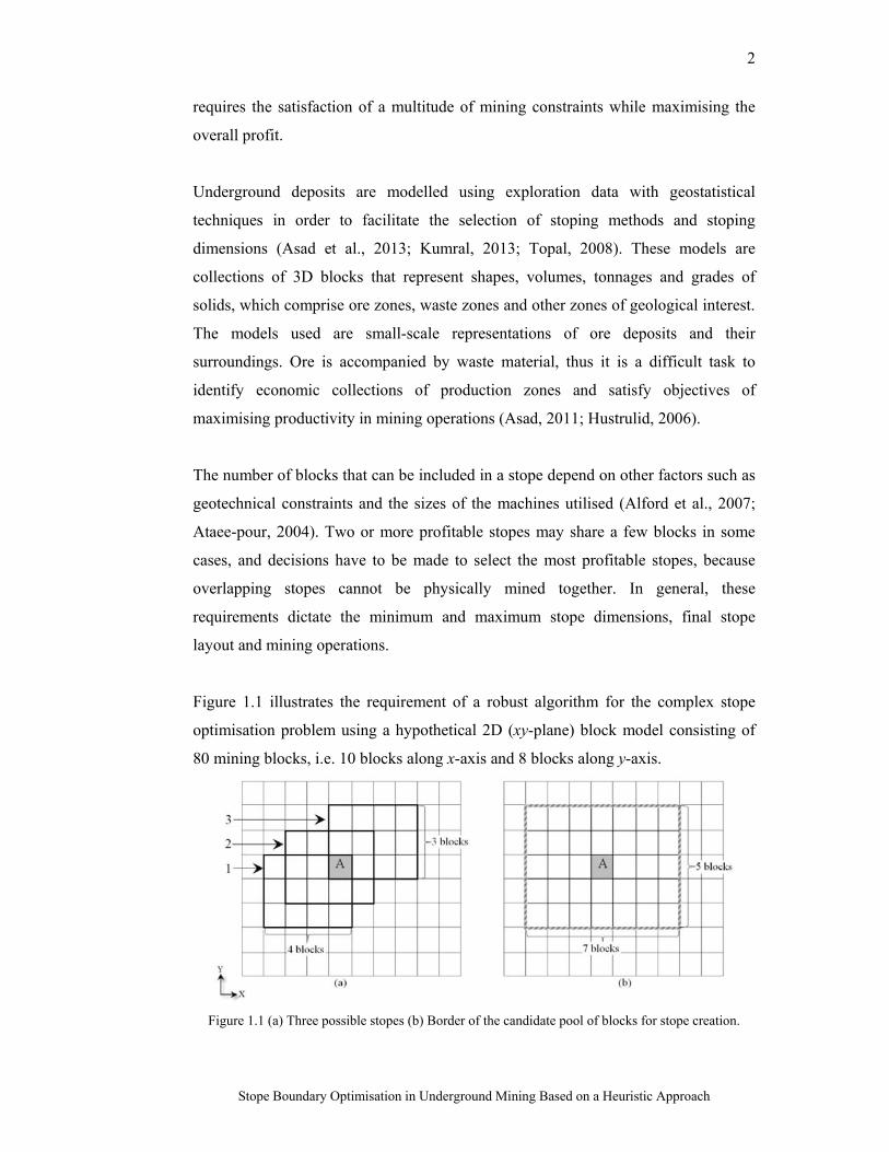
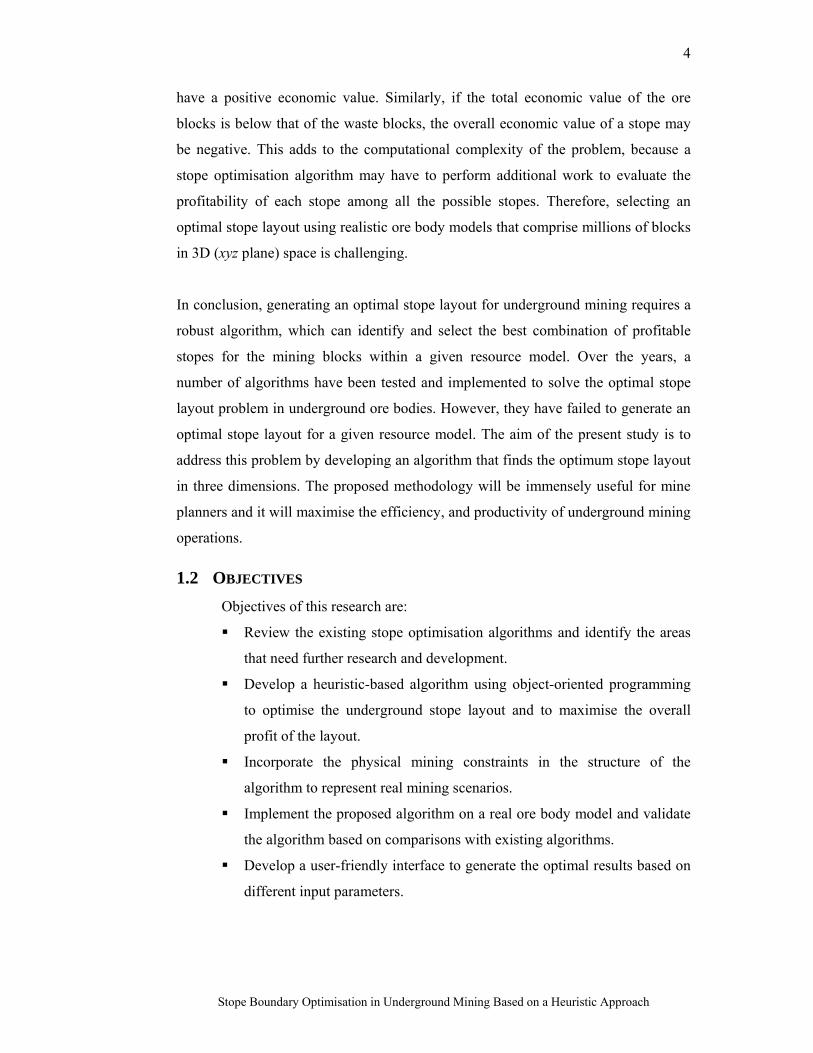
Figure 1.1 illustrates the requirement of a robust algorithm for the complex stope
optimisation problem using a hypothetical 2D (xy-plane) block model consisting of
80 mining blocks, i.e. 10 blocks along x-axis and 8 blocks along y-axis.
Figure 1.1 (a) Three possible stopes (b) Border of the candidate pool of blocks for stope creation.
3
Stope Boundary Optimisation in Underground Mining Based on a Heuristic Approach
In this hypothetical situation, the mining constraints restrict the stope size to four
blocks along the x axis and three blocks along the y axis, i.e., a total of 12 mining
blocks inside a stope. Consequently, Figure 1.1 (a) shows that there are three
possible stopes around a given mining block A. Figure 1.1 (b) indicates the boundary
of a candidate pool of 35 mining blocks, i.e., seven blocks along the x dimension and
five blocks along the y axis, where 11 blocks can be aggregated with mining block A
to create stopes that satisfy the stope size constraint. If the z axis is also considered,
the candidate pool of blocks expands further and the stope boundary becomes much
larger. However, mining block A may belong to a single stope, because it is not
physically possible to mine overlapping stopes in underground mining situations.
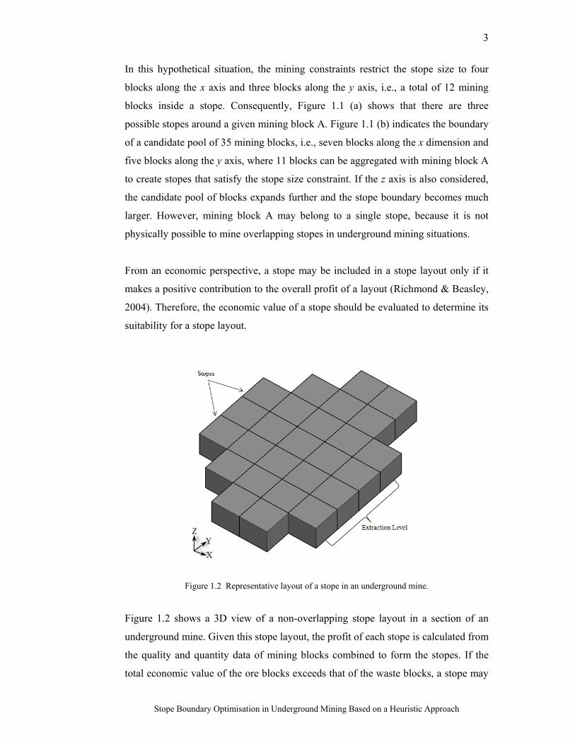
From an economic perspective, a stope may be included in a stope layout only if it
makes a positive contribution to the overall profit of a layout (Richmond & Beasley,
2004). Therefore, the economic value of a stope should be evaluated to determine its
suitability for a stope layout.
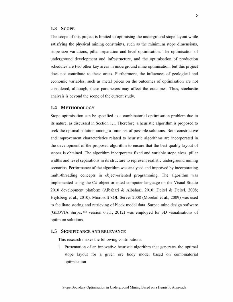
Figure 1.2 Representative layout of a stope in an underground mine.
Figure 1.2 shows a 3D view of a non-overlapping stope layout in a section of an
underground mine. Given this stope layout, the profit of each stope is calculated from
the quality and quantity data of mining blocks combined to form the stopes. If the
total economic value of the ore blocks exceeds that of the waste blocks, a stope may
4
Stope Boundary Optimisation in Underground Mining Based on a Heuristic Approach
have a positive economic value. Similarly, if the total economic value of the ore
blocks is below that of the waste blocks, the overall economic value of a stope may
be negative. This adds to the computational complexity of the problem, because a
stope optimisation algorithm may have to perform additional work to evaluate the
profitability of each stope among all the possible stopes. Therefore, selecting an
optimal stope layout using realistic ore body models that comprise millions of blocks
in 3D (xyz plane) space is challenging.
In conclusion, generating an optimal stope layout for underground mining requires a
robust algorithm, which can identify and select the best combination of profitable
stopes for the mining blocks within a given resource model. Over the years, a
number of algorithms have been tested and implemented to solve the optimal stope
layout problem in underground ore bodies. However, they have failed to generate an
optimal stope layout for a given resource model. The aim of the present study is to
address this problem by developing an algorithm that finds the optimum stope layout
in three dimensions. The proposed methodology will be immensely useful for mine
planners and it will maximise the efficiency, and productivity of underground mining
operations.
1.2 OBJECTIVES
Objectives of this research are:
Review the existing stope optimisation algorithms and identify the areas
that need further research and development.
Develop a heuristic-based algorithm using object-oriented programming
to optimise the underground stope layout and to maximise the overall
profit of the layout.
Incorporate the physical mining constraints in the structure of the
algorithm to represent real mining scenarios.
Implement the proposed algorithm on a real ore body model and validate
the algorithm based on comparisons with existing algorithms.
Develop a user-friendly interface to generate the optimal results based on
different input parameters.
5
Stope Boundary Optimisation in Underground Mining Based on a Heuristic Approach
1.3 SCOPE
The scope of this project is limited to optimising the underground stope layout while
satisfying the physical mining constraints, such as the minimum stope dimensions,
stope size variations, pillar separation and level optimisation. The optimisation of
underground development and infrastructure, and the optimisation of production
schedules are two other key areas in underground mine optimisation, but this project
does not contribute to these areas. Furthermore, the influences of geological and
economic variables, such as metal prices on the outcomes of optimisation are not
considered, although, these parameters may affect the outcomes. Thus, stochastic
analysis is beyond the scope of the current study.
1.4 METHODOLOGY
Stope optimisation can be specified as a combinatorial optimisation problem due to
its nature, as discussed in Section 1.1. Therefore, a heuristic algorithm is proposed to
seek the optimal solution among a finite set of possible solutions. Both constructive
and improvement characteristics related to heuristic algorithms are incorporated in
the development of the proposed algorithm to ensure that the best quality layout of
stopes is obtained. The algorithm incorporates fixed and variable stope sizes, pillar
widths and level separations in its structure to represent realistic underground mining
scenarios. Performance of the algorithm was analysed and improved by incorporating
multi-threading concepts in object-oriented programming. The algorithm was
implemented using the C# object-oriented computer language on the Visual Studio
2010 development platform (Albahari & Albahari, 2010; Deitel & Deitel, 2008;
Hejlsberg et al., 2010). Microsoft SQL Server 2008 (Morelan et al., 2009) was used
to facilitate storing and retrieving of block model data. Surpac mine design software
(GEOVIA Surpac™ version 6.3.1, 2012) was employed for 3D visualisations of
optimum solutions.
1.5 SIGNIFICANCE AND RELEVANCE
This research makes the following contributions:
1. Presentation of an innovative heuristic algorithm that generates the optimal
stope layout for a given ore body model based on combinatorial
optimisation.
6
Stope Boundary Optimisation in Underground Mining Based on a Heuristic Approach
2. An algorithm which overcomes the computational complexity by reducing
the set of infinite solutions to a discrete set of finite solutions in order to find
the best solution.
3. An algorithm that introduces an innovative method for identifying
overlapping stopes and avoiding their inclusion in the optimum stope layout.
4. An implementation of the task-parallelism concept in object-oriented
programming to improve the performance of the proposed stope optimisation
algorithm.
5. An algorithm which incorporates important stope optimisation
characteristics, including pillar separation, level separation and stope size
variation, to generate solutions representing realistic underground mining
scenarios.
6. Alterations to the configuration of input demonstrate further improvements
to the solution values.
7. Implementation of the algorithm using Microsoft C# object-oriented
programming language enables the execution of the application on windows-
based computers with different architectures and/or platforms.
8. A user-friendly interface which enables rapid implementations of the stope
optimisation algorithm in various mining scenarios.
1.6 THESIS OVERVIEW
Chapter 1 presents an introduction to the stope optimisation problem, including
descriptions of its complexity, project objectives, scope, methodology and the
significance of the project for the mining industry.
Chapter 2 presents an in-depth review of the existing stope optimisation algorithms.
Furthermore, it includes a discussion about the applications of heuristics in
combinatorial optimisation and their relevance to the stope optimisation problem.
Chapter 3 explains the proposed algorithm for stope boundary optimisation,
including the general flow of the algorithm, improvements for different mining
scenarios and modifications that address the computational complexity of the
problem.
Chapter 4 presents an implementation of the proposed algorithm for an authentic
resource model. Based on six cases, the applicability of the algorithm to different
7
Stope Boundary Optimisation in Underground Mining Based on a Heuristic Approach
mining scenarios is demonstrated. Furthermore, it includes a validation study of the
proposed algorithm.
Chapter 5 concludes the outcomes, analyses the performance of the proposed
algorithm, and provides recommendations for future research.
8
Stope Boundary Optimisation in Underground Mining Based on a Heuristic Approach
CHAPTER 2 UNDERGROUND STOPE
OPTIMISATION
A variety of mine optimisation techniques have been developed since the early
1960s, and surface mine planning and design have improved remarkably as a result.
For example, the current commercially available Lerchs-Grossmann algorithm has
been implemented successfully to determine the ultimate pit limits for an open pit
mine operation. By contrast, underground stope optimisation has received little
attention. The lack of tools and appropriate computer programs to address
underground mining problems remains an issue (Alford & Hall, 2009; Little &
Topal, 2011).
An optimum stope layout dictates the maximisation of net present value in
subsequent production scheduling, which is critical when planning an underground
mining project (Hustrulid & Bullock, 2001; Kumral, 2010). Stope optimisation is far
more complex than open pit mining optimisation with various mining methods being
used in underground mining and their applications varying among mine sites. Further
underground mining projects may require employment of more than one mining
method when the ore body has a complex geometry, to improve safety and
production. Furthermore, the development of underground stopes requires the
consideration of physical and geotechnical constraints, for instance, the size of
mining equipment, extent of mine development levels that provide access to the
stopes, size and orientation of the ore body size of ore pillars which ensure stability
of underground production areas (Gertch & Bullock, 1998; Krishna & Chanda,
1997). These parameters also affect the design of the dimensions (width, height and
length) of stopes.
Geometrically, there are numerous possible options for the removal of a particular
mining block relative to underground mining, as mentioned in Section 1.1 of Chapter
1. However, for a given slope angle constraint, there is only one possible option for
removing a particular block in an open pit mine, thus generating an ultimate pit limit
which is not as computationally complex as selecting the optimum stope layout for
9
Stope Boundary Optimisation in Underground Mining Based on a Heuristic Approach
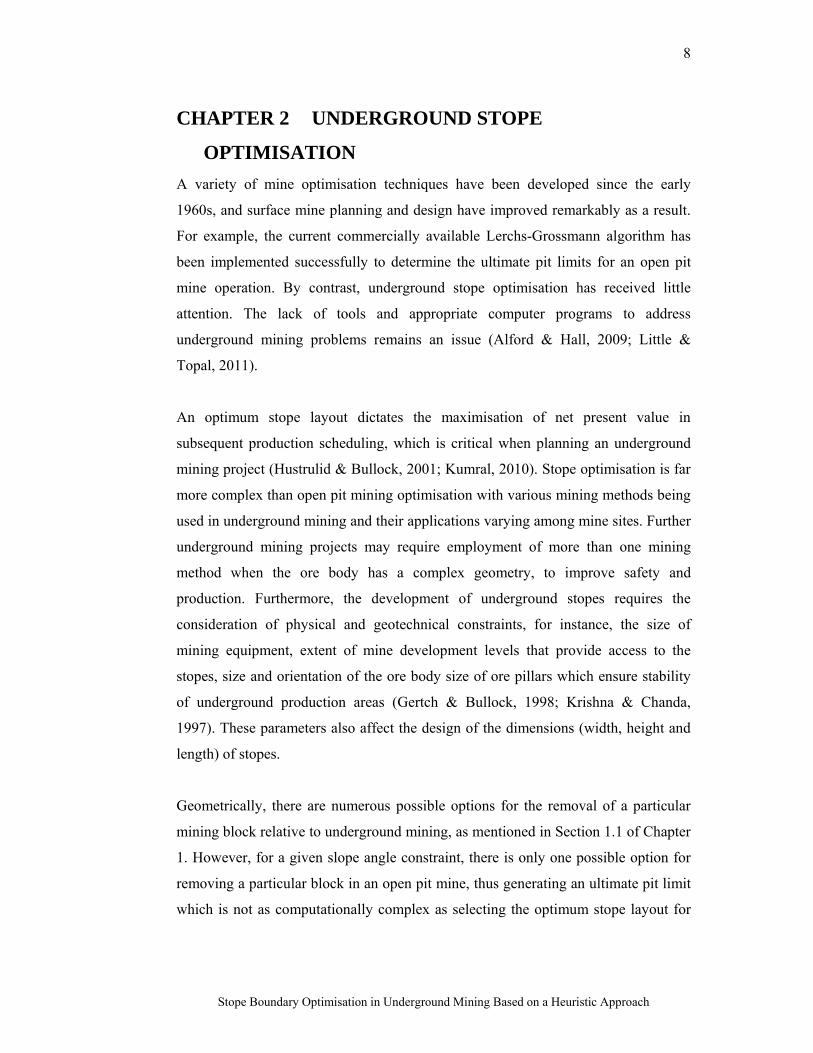
underground mining. Figure 2.1 shows a two-dimensional (2D) hypothetical situation
that illustrates the simplicity of block removal during open pit mining.
Figure 2.1 Two-dimensional view of an open pit mining geometry.
Given a slope angle of45° , the space (shaded blocks in Figure 2.1) required to
remove mining block A is a unique inverted cone (Ataee-pour, 2005). Altering the
slope angle may result in a change in the size of the cone, however, for the given
angle of 45°, there is only one solution.
Section 2.1 provides an overview of the stoping methods to which the proposed
algorithm is applicable. Section 2.2 reviews the existing algorithms and describes
their advantages and disadvantages in detail. Finally, Section 2.10 explains the role
of heuristic algorithms in solving combinatorial optimisation problems.
2.1 FUNDAMENTALS OF STOPING METHODS
Stoping is a systematic engineering process that involves extracting valuable ore
from an underground mine using specific mining methods. The selection of an
underground stoping method is largely based on the spatial orientation of a given ore
body. Operational/capital costs, production rates, labour availability, ground support
and considerations for equipment also play a vital role in the selection of a stoping
method. The fundamental aim is to select a method that offers the best combination
of operational safety, production economics and mining recovery (Okubo &
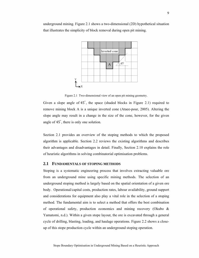
Yamatomi, n.d.). Within a given stope layout, the ore is excavated through a general
cycle of drilling, blasting, loading, and haulage operations. Figure 2.2 shows a close-
up of this stope production cycle within an underground stoping operation.
10
Stope Boundary Optimisation in Underground Mining Based on a Heuristic Approach
Figure 2.2 A close-up of production operations with a stope of an underground mine (Gertch and Bullock, 1998).
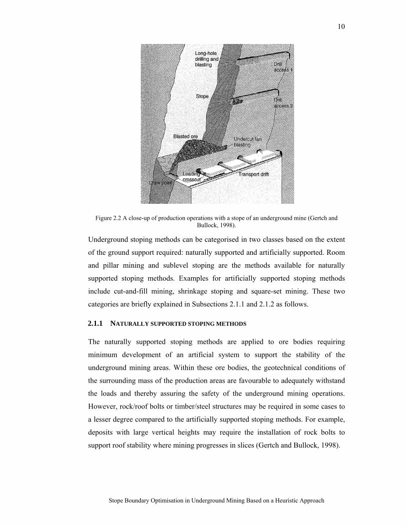
Underground stoping methods can be categorised in two classes based on the extent
of the ground support required: naturally supported and artificially supported. Room
and pillar mining and sublevel stoping are the methods available for naturally
supported stoping methods. Examples for artificially supported stoping methods
include cut-and-fill mining, shrinkage stoping and square-set mining. These two
categories are briefly explained in Subsections 2.1.1 and 2.1.2 as follows.
2.1.1 NATURALLY SUPPORTED STOPING METHODS The naturally supported stoping methods are applied to ore bodies requiring
minimum development of an artificial system to support the stability of the
underground mining areas. Within these ore bodies, the geotechnical conditions of
the surrounding mass of the production areas are favourable to adequately withstand
the loads and thereby assuring the safety of the underground mining operations.
However, rock/roof bolts or timber/steel structures may be required in some cases to
a lesser degree compared to the artificially supported stoping methods. For example,
deposits with large vertical heights may require the installation of rock bolts to
support roof stability where mining progresses in slices (Gertch and Bullock, 1998).
11
Stope Boundary Optimisation in Underground Mining Based on a Heuristic Approach
Among naturally supported stoping methods, room-and-pillar mining is used for
deposits with limited thickness such as coal, limestone, and shale. The sublevel
stoping mining method is applied to vertical or steeply inclined ore bodies.
2.1.2 ARTIFICIALLY SUPPORTED STOPING METHODS The artificially supported stoping methods are employed for the extraction of ore
bodies which require a higher degree of ground control systems. The load-carrying
capacity of the rock mass in these ore bodies is not sufficient to sustain safety of the
underground operations and openings. As such, support structures are provided in
terms of timbers, backfilling, cribs, and hydraulics to improve stability of
underground mining (Hustrulid & Bullock, 2001).
Among artificially supported stoping methods, Cut-and-fill mining exploits the ore
body in horizontal slices generally from the bottom of a stope upwards similar to
shrinkage stoping. This method is applied to steeply dipping ore bodies which are
moderately competent. Waste rock may be utilised as fill material though in the
modern practice, hydraulic filling methods are used. Shrinkage stoping guides ore
extraction from the bottom of a stope upwards in terms of horizontal slices. This
method is best utilised for steeply dipping ore bodies. Square-set mining is most
suitable for small high-grade ore bodies and based on timber-support structures.
Though it can be applied to any orebody shape and ground condition, it demands a
steady supply of timbers and intensive labour. In some cases, variations of sublevel
stoping are categorised in to artificially supported stoping methods when the pillars
are recovered and the voids are filled with hydraulic fill, paste or cemented rock
(Darling, 2011).
2.2 THE EXISTING STOPE OPTIMISATION ALGORITHMS
The few existing algorithms for optimising stope layouts may be classified as
rigorous and heuristic (Ataee-pour, 2005). Rigorous algorithms are supported by
mathematical proofs, and some examples of this category include the dynamic
programming algorithm (Riddle, 1977), branch and bound technique (Ovanic &
Young, 1995) and network flow method (Bai et al., 2013). Heuristic approaches
solve optimality problems based on rules that are applied during the search of
optimal stope layouts. Examples also include the octree division algorithm
(Cheimanoff et al., 1989), floating stope algorithm (Alford, 1995), Sens and Topal
12
Stope Boundary Optimisation in Underground Mining Based on a Heuristic Approach
heuristic approach (Sens & Topal, 2009) and maximum value neighbourhood
algorithm (Ataee-pour, 2000).
2.2.1 DYNAMIC PROGRAMMING SOLUTION FOR STOPE OPTIMISATION Riddle (1977) proposed a dynamic programming-based solution for defining stope
boundaries in block caving-related mining systems. During initialisation, the
algorithm assumes that there is no footwall in the optimisation process and that the
maximum profit is achieved irrespective of the footwall design. Next, it defines a
footwall in operational regions and examines the profitability of all feasible solutions
for mining and non-mining regions. In the subsequent steps, the process divides the
defined footwall region into two sub-regions if the profit is greater than or equal to
an assumed profit. The process terminates when there are no more profitable
footwalls to examine, or no further feasible footwalls can be introduced into the
operational region. This 2D approach is useful for the stope optimisation problem
because of its simplicity, but it does not support the realistic 3D mining situations.
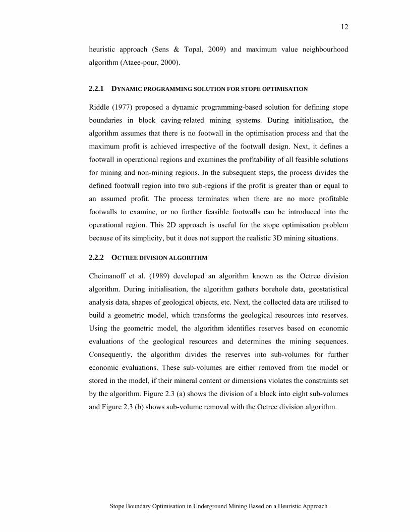
2.2.2 OCTREE DIVISION ALGORITHM Cheimanoff et al. (1989) developed an algorithm known as the Octree division
algorithm. During initialisation, the algorithm gathers borehole data, geostatistical
analysis data, shapes of geological objects, etc. Next, the collected data are utilised to
build a geometric model, which transforms the geological resources into reserves.
Using the geometric model, the algorithm identifies reserves based on economic
evaluations of the geological resources and determines the mining sequences.
Consequently, the algorithm divides the reserves into sub-volumes for further
economic evaluations. These sub-volumes are either removed from the model or
stored in the model, if their mineral content or dimensions violates the constraints set
by the algorithm. Figure 2.3 (a) shows the division of a block into eight sub-volumes
and Figure 2.3 (b) shows sub-volume removal with the Octree division algorithm.
13
Stope Boundary Optimisation in Underground Mining Based on a Heuristic Approach
Figure 2.3 (a) Octree division. (b) Successive removal of sub-volumes (Cheimanoff et al., 1989).
The Octree division algorithm generates a 3D feasible solution for the stope
geometry, but it leads to more waste being added in the final mine layout because the
algorithm does not analyse the sub-volumes jointly. It includes individual sub-
volumes that consider the minimum allowable dimensions in the final layout but not
the amount of waste in these sub-volumes. As such, the algorithm does not guarantee
the optimality of stope layouts.
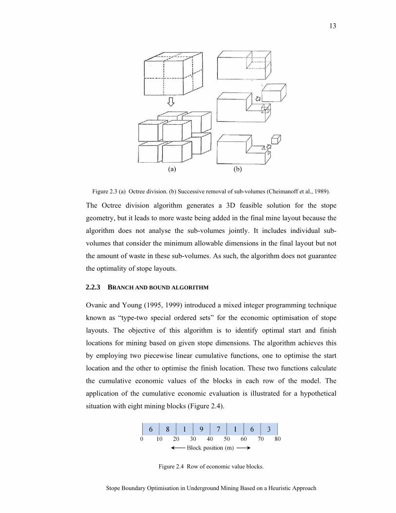
2.2.3 BRANCH AND BOUND ALGORITHM Ovanic and Young (1995, 1999) introduced a mixed integer programming technique
known as “type-two special ordered sets” for the economic optimisation of stope
layouts. The objective of this algorithm is to identify optimal start and finish
locations for mining based on given stope dimensions. The algorithm achieves this
by employing two piecewise linear cumulative functions, one to optimise the start
location and the other to optimise the finish location. These two functions calculate
the cumulative economic values of the blocks in each row of the model. The
application of the cumulative economic evaluation is illustrated for a hypothetical
situation with eight mining blocks (Figure 2.4).
Figure 2.4 Row of economic value blocks.
Stop
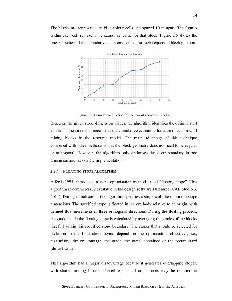
The block
within eac
linear func
Based on
and finish
mining b
compared
or orthogo
dimension
2.2.4 FL
Alford (19
algorithm
2014). Du
dimension
defined flo
the grade
that fall w
inclusion
maximisin
(dollar) va
This algor
with shar
pe Boundary O
ks are repre
ch cell repr
ction of the
Figure
the given st
locations th
locks in th
with other
onal. Howe
n and lacks a
LOATING ST
995) introdu
is commerc
uring initiali
ns. The spec
oat increme
inside the f
within this s
in the fin
ng the ore
alue.
rithm has a
red mining
Optimisation i
sented in b
resent the e
cumulative
e 2.5 Cumulat
tope dimen
hat maximi
he resource
methods is
ever, the al
a 3D implem
OPE ALGOR
uced a stop
cially availa
isation, the
cified stope
ents in three
floating stop
pecified sto
nal stope la
tonnage, th
a major dis
blocks. Th
in Undergroun
blue colour
economic va
e economic
tive function f
sion values
ses the cum
e model. T
s that the blo
lgorithm on
mentation.
RITHM
pe optimisat
able in the d
algorithm s
e is floated i
e orthogona
pe is calcula
ope boundar
ayout depen
he grade, t
sadvantage
herefore, m
nd Mining Ba
cells and sp
alue for tha
values for e
for the row of
, the algorit
mulative eco
The main
ock geomet
nly optimise
tion method
design softw
specifies a
in the ore b
al direction
ated by aver
ry. The stop
nd on the
the metal c
because it
manual adju
ased on a Heur
paced 10 m
at block. Fi
each sequen
f economic blo
thm identifi
onomic func
advantage
try does not
es the stop
d called “fl
ware Datam
stope with
body relativ
s. During th
raging the g
pes that sho
optimisatio
contained o
generates o
ustments m
ristic Approac
m apart. The
gure 2.5 sh
ntial block p
ocks.
ies the optim
ction of each
of this te
t need to be
pe boundary
loating stop
mine (CAE S
the minimu
ve to an orig
he floating
grades of th
ould be sele
on objectiv
or the accu
overlapping
may be requ
14
ch
e figures
hows the
position.
mal start
h row of
echnique
e regular
y in one
pe”. This
Studio 3,
um stope
gin, with
process,
he blocks
ected for
ves, i.e.,
umulated
g stopes,
uired to
15
Stope Boundary Optimisation in Underground Mining Based on a Heuristic Approach
exclude these shared blocks from the final layout, because a block cannot physically
belong to multiple stopes. Consequently, the economic values of the shared blocks
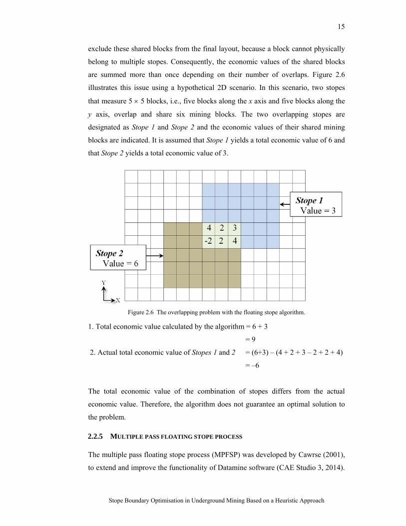
are summed more than once depending on their number of overlaps. Figure 2.6
illustrates this issue using a hypothetical 2D scenario. In this scenario, two stopes
that measure 5 5 blocks, i.e., five blocks along the x axis and five blocks along the
y axis, overlap and share six mining blocks. The two overlapping stopes are
designated as Stope 1 and Stope 2 and the economic values of their shared mining
blocks are indicated. It is assumed that Stope 1 yields a total economic value of 6 and
that Stope 2 yields a total economic value of 3.
Figure 2.6 The overlapping problem with the floating stope algorithm.
1. Total economic value calculated by the algorithm = 6 + 3
= 9
2. Actual total economic value of Stopes 1 and 2 = (6+3) – (4 + 2 + 3 – 2 + 2 + 4)
= –6
The total economic value of the combination of stopes differs from the actual
economic value. Therefore, the algorithm does not guarantee an optimal solution to
the problem.
2.2.5 MULTIPLE PASS FLOATING STOPE PROCESS The multiple pass floating stope process (MPFSP) was developed by Cawrse (2001),
to extend and improve the functionality of Datamine software (CAE Studio 3, 2014).
16
Stope Boundary Optimisation in Underground Mining Based on a Heuristic Approach
The MPFSP process is divided into three steps: input parameter definition, file
generation and file management. Input parameters such as the head grade, cut-off
grade and maximum waste are defined by the user. During the file generation step,
economic stope envelopes are created for each set of parameters. Finally, the data
files or the statistical files generated in the process are converted into a Microsoft
Excel compatible (CSV) format.
Subsequently, the MPFSP process provides an informative evaluation of the block
model examining the stoping feasibility and identifying possible areas for the
development of stopes. However, it does not eliminate the shortcomings of the
“floating stope” algorithm. The method can facilitate stope boundary selection and
design but it does not generate optimum stope layouts (Cawrse, 2007).
2.2.6 MAXIMUM VALUE NEIGHBOURHOOD ALGORITHM Ataee-pour (2000) developed an algorithm based on a heuristic approach called the
maximum value neighbourhood (MVN). The algorithm defines a number of mining
blocks that should be mined together to satisfy the minimum stope size constraint.
Next, sets of feasible neighbourhoods are identified for each block of the model. The
economic value of each neighbourhood is determined to identify the MVN, i.e., the
neighbourhood with the maximum economic value. Finally, all of the MVN blocks
are flagged for inclusion in the final stope layout. Some checks are performed to
ensure the exclusion of waste blocks, and consequently, an enhancement in the
performance of the algorithm. For example, if a block is already flagged or if a block
has a negative value, the algorithm terminates the neighbourhood evaluation process
for that particular block.
The MVN algorithm has advantages in terms of its simple concept and
computational implementation, but it also has several drawbacks. First, the algorithm
identifies a collection of MVNs rather than mineable stopes. The algorithm defines
the neighbourhood dimensions based on a minimum stope width requirement, but in
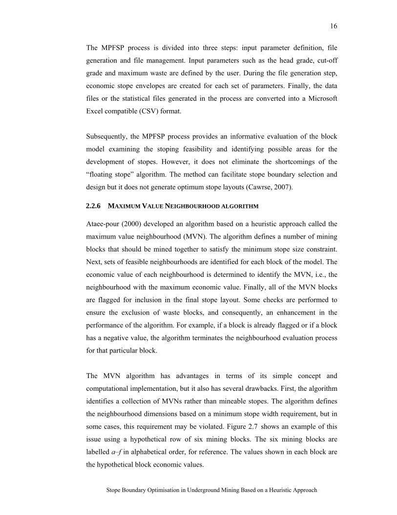
some cases, this requirement may be violated. Figure 2.7 shows an example of this
issue using a hypothetical row of six mining blocks. The six mining blocks are
labelled a–f in alphabetical order, for reference. The values shown in each block are
the hypothetical block economic values.
17
Stope Boundary Optimisation in Underground Mining Based on a Heuristic Approach
Figure 2.7 Example illustrating the main problem with the MVN algorithm.
According to this hypothetical example, a neighbourhood of three blocks is defined
as the minimum stope size. The algorithm derives two MVNs, which comprise
blocks b, c, d and e. However, selecting either of the neighbourhoods may result in
violation of the minimum stope width constraint. For example, if neighbourhood (i)
is selected from step 2, mining of block b may be impossible because it is a single
block, thus it violates the minimum stope size constraint. Similarly, mining of block
e may be impossible, if neighbourhood (ii) is selected from step 3. Therefore, the
implementation of the algorithm does not yield a practical mining solution for the
stope optimisation problem. Furthermore, the algorithm generates different outcomes
depending on the selection of the start point, thereby indicating that the algorithm
18
Stope Boundary Optimisation in Underground Mining Based on a Heuristic Approach
cannot ensure that the best solution to the problem is obtained (Little, 2012; Little et
al., 2013).
2.2.7 MIXED INTEGER PROGRAMMING-BASED ALGORITHM Grieco and Dimitrakopoulos (2007) developed a probabilistic optimisation algorithm
based on mixed integer programming. In this approach, the ore body is divided into
layers initially. Each layer is then subdivided into a number of panels and each panel
is subdivided into a series of rings. Each ring is assigned to a binary variable of the
mixed integer model. The objective function of the algorithm works by maximising
the metal content at a given time. The minimum and maximum mining rings, and the
sizes of the pillars that need to be left unmined between two primary stopes, are
limited by the constraints of the model. This method considers the geological
uncertainty during the stope design stage, but it does not allow accurate examinations
of stopes in different locations. It generates the optimum stope layout based on the
rings that are defined relative to the location and size of the most profitable stopes.
Further, the algorithm does not ensure precise examination of stopes in different
locations of the ore body. Furthermore, the performance of the algorithm is
proportional to the number of binary variables in the mixed integer model, causing
the solution time to increase as the number of rings increase (Dimitrakopoulos &
Grieco, 2009).
2.2.8 SENS AND TOPAL HEURISTIC APPROACH Sens and Topal (2009) introduced a new algorithm based on a heuristic approach.
During initialisation, the given mining block model is converted to a regularised
block model, i.e., a block model that constitutes mining blocks with consistent sizes.
Given the dimensions (height, length and width) stopes are generated from the
regularised block model. Finally a heuristic stope optimisation algorithm is
implemented in Matlab software based on the economic value of stopes and the
results are visualised with respect to different user-defined parameters. The
advantage is that it locates stope boundaries using different stope sizes and selection
strategies in three dimensions.
To its disadvantage, the algorithm selects the stopes in descending order of the stope
economic values while removing the overlapping stopes. To clarify, this process
19
Stope Boundary Optimisation in Underground Mining Based on a Heuristic Approach
discards the possibility of multiple stope combinations that can be derived from a
given stope set. Amongst these multiple combinations, there may be combinations
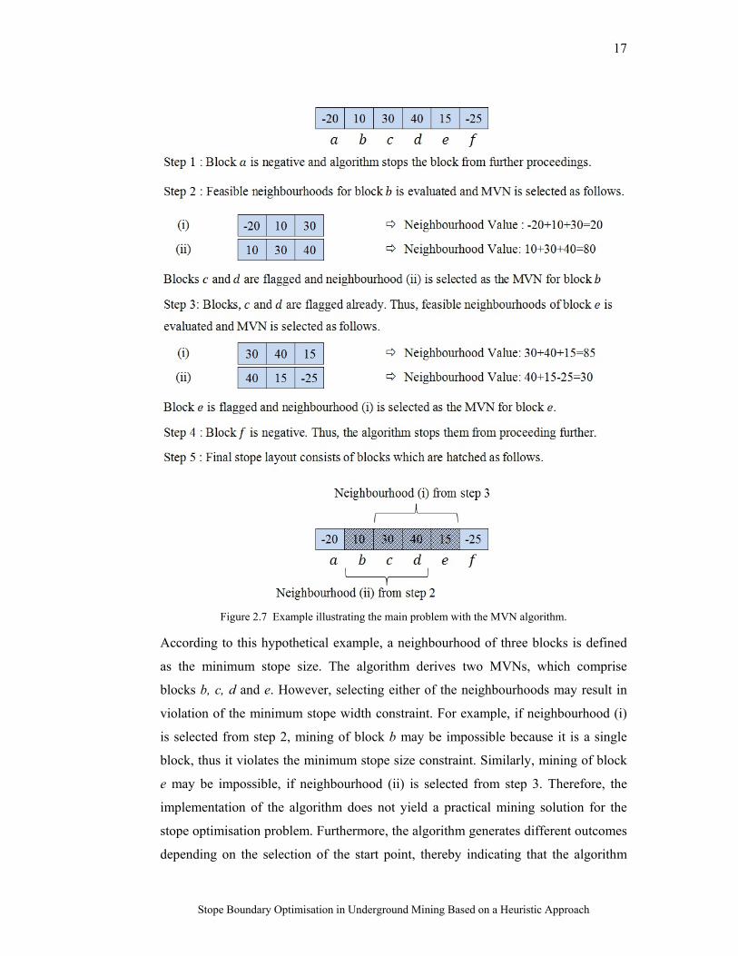
with higher total economic values. Figure 2.8 illustrates this problem based on a
hypothetical situation. In this 2D diagram, the stope size is fixed at 5 4, i.e., five
blocks along the x axis and four blocks along the y axis.
Figure 2.8 The problem with Sens and Topal heuristic approach.
1. Combination selected by the algorithm = Stope 1 and Stope 2
(Total economic value= 10 + 5 = 15)
2. Most profitable combination = Stope 3 and Stope 4
(Total economic value = 8 + 9 = 17)
Therefore, the final stope selection criterion employed by this algorithm fails to
generate the most profitable stope combination.
2.2.9 NETWORK FLOW METHOD Bai et al. (2013) introduced the graph theory and network flow method for
underground stope optimisation. This approach was implemented specifically for
underground mines that operate using the sub-level stoping mining method. The
algorithm specifies an initial location and extent for development of a raise, before
defining a cylindrical coordinate system around the specified raise location. The
cylindrical system establishes the precedence links between mining blocks, which are
required to satisfy the geotechnical constraints on the footwall and the hanging wall
slopes. Figure 2.9 (a) shows a block model using the cylindrical coordinate system.
Figure 2.9 (b) shows the arcs with vertical links of precedence for a given block A,
20
Stope Boundary Optimisation in Underground Mining Based on a Heuristic Approach
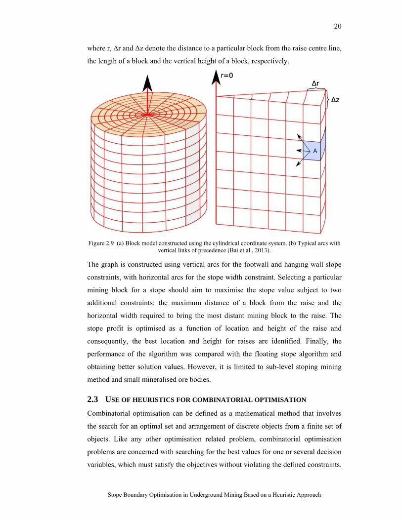
where r, Δr and Δz denote the distance to a particular block from the raise centre line,
the length of a block and the vertical height of a block, respectively.
Figure 2.9 (a) Block model constructed using the cylindrical coordinate system. (b) Typical arcs with
vertical links of precedence (Bai et al., 2013).
The graph is constructed using vertical arcs for the footwall and hanging wall slope
constraints, with horizontal arcs for the stope width constraint. Selecting a particular
mining block for a stope should aim to maximise the stope value subject to two
additional constraints: the maximum distance of a block from the raise and the
horizontal width required to bring the most distant mining block to the raise. The
stope profit is optimised as a function of location and height of the raise and
consequently, the best location and height for raises are identified. Finally, the
performance of the algorithm was compared with the floating stope algorithm and
obtaining better solution values. However, it is limited to sub-level stoping mining
method and small mineralised ore bodies.
2.3 USE OF HEURISTICS FOR COMBINATORIAL OPTIMISATION
Combinatorial optimisation can be defined as a mathematical method that involves
the search for an optimal set and arrangement of discrete objects from a finite set of
objects. Like any other optimisation related problem, combinatorial optimisation
problems are concerned with searching for the best values for one or several decision
variables, which must satisfy the objectives without violating the defined constraints.
21
Stope Boundary Optimisation in Underground Mining Based on a Heuristic Approach
However, most combinatorial optimisation problems are NP-hard, as defined in
computational complexity theory, meaning it is often impossible to solve the
instances in reasonable time (Karapetyan, 2010). Implementation of exact
optimisation algorithms may also be impossible because many modern optimisation
problems tend to be complex and require analysis of large data sets. Two examples
of NP-hard problems are stated as follows.
1. The travelling salesman problem (TSP): Given a list of cities and their spatial
coordinates where an origin city is defined, find the shortest possible route that visits
each city once and only once, and returns to the city of origin (Basel & Willemain,
2001; Lam & Newman, 2008; Punnen, 2007).
2. The subset sum problem (SSP): Given a set of integers , , … and is
an integer number, determine whether there exists a subset of 1,2,… , such that
∑ ∈ , i.e., determine whether there exists a set ⊂ where the sum of the
members of is (Bernstein et al., 2013).
In both cases, finding the optimal solution, i.e., the shortest route in the case of TSP
and a set with sum in the case of SSP requires search methods to select the
optimal solution among a set of possible solutions. However, as the problem size
increases, i.e., number of cities in TSP and the cardinality (number of members) of
set in SSP, the search for possible solutions becomes intense and exhaustive. In
such cases, heuristic algorithms are essential because they may generate a near-
optimal solution for a given NP-hard problem. In some cases, they may be the only
practical alternative for NP-hard optimisation problems, subject to computational
complexity, problem size and solution time constraints (Gonçalves & Resende,
2011;Martí et al., 2013;Rardin & Uzsoy, 2001).
2.3.1 TYPES OF HEURISTIC ALGORITHMS Heuristic algorithms may be used to build a solution constructively (piece by piece)
or by progressive improvements (Semančo & Modrák, 2011;Žerovnik & Žerovnik,
2011). Many constructive heuristics are “greedy”, which means they take the best
solution without regard for the remaining solutions. For example, a constructive
approach to the TSP is to take the nearest city in consecutive steps. Similarly, a
constructive approach for the SSP would be to randomly select an ∈ and to
22
Stope Boundary Optimisation in Underground Mining Based on a Heuristic Approach
search for any ∈ from a set ⊂ . The objective is to ensure that the
cardinality of , i.e., the number of members of , remains as low as possible to
address the computational complexity, which may be caused by the cardinality of .
By contrast, improvement heuristics are “intelligent”, which means that they employ
techniques to obtain better quality solutions using the given specified objects. An
example of an improvement approach would be to generate a possible solution for
TSP and then to swap the order of a few cities to generate a better solution. A
possible improvement approach for the SSP is to randomly select any ∈ and
then to search for any ∈ such that ≅ . The objective of this approach
is to find any better value for from set such that is as close as possible to
zero.
In general, a heuristic algorithm can be compound in nature, i.e., a combination of
constructive and improvement types. A compound heuristic solves an NP-hard
optimisation problem in two phases: a constructive phase followed by an
improvement phase (Derigs & Vogel, 2014).
2.4 SUMMARY
Numerous approaches have been developed to solve the stope optimisation problem,
but none of them guarantees the generation of an optimal solution that satisfies the
physical mining constraints in 3D space. Therefore, stope optimisation for
underground mining requires a robust algorithm that can handle the computational
complexity and satisfy the physical mining constraints to generate an optimal
solution.
According to the concepts employed by combinatorial optimisation in operations
research, the stope optimisation problem can be defined as an NP-hard optimisation
problem because of its computational complexity and the problem size. Therefore,
this problem may be addressed using a heuristic algorithm that searches for the
possible solutions and finds the optimal solution among them while satisfying the
physical mining constraints. The constructive and improvement characteristics
discussed in Subsection 2.10.1 are incorporated into the proposed algorithm to
generate better quality solutions in the least possible time.
23
Stope Boundary Optimisation in Underground Mining Based on a Heuristic Approach
CHAPTER 3 DEVELOPMENT OF THE PROPOSED
ALGORITHM
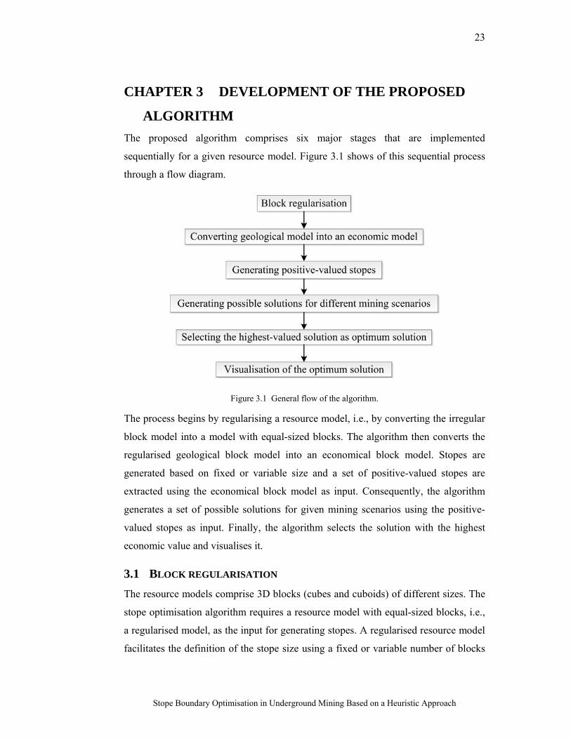
The proposed algorithm comprises six major stages that are implemented
sequentially for a given resource model. Figure 3.1 shows of this sequential process
through a flow diagram.
Figure 3.1 General flow of the algorithm.
The process begins by regularising a resource model, i.e., by converting the irregular
block model into a model with equal-sized blocks. The algorithm then converts the
regularised geological block model into an economical block model. Stopes are
generated based on fixed or variable size and a set of positive-valued stopes are
extracted using the economical block model as input. Consequently, the algorithm
generates a set of possible solutions for given mining scenarios using the positive-
valued stopes as input. Finally, the algorithm selects the solution with the highest
economic value and visualises it.
3.1 BLOCK REGULARISATION
The resource models comprise 3D blocks (cubes and cuboids) of different sizes. The
stope optimisation algorithm requires a resource model with equal-sized blocks, i.e.,
a regularised model, as the input for generating stopes. A regularised resource model
facilitates the definition of the stope size using a fixed or variable number of blocks
24
Stope Boundary Optimisation in Underground Mining Based on a Heuristic Approach
from x, y and z axes, thus a given ore body model is regularised at the beginning of
the stope optimisation process.
The dimensions (length, width, and height) of the regularised blocks are defined by
the algorithm. The minimum coordinate among the set of coordinates for the original
blocks becomes the minimum coordinate of the regularised block model. Similarly,
the maximum coordinate among the set of coordinates for the original blocks
becomes the maximum coordinate of the regularised block model. After defining the
new dimensions and the two limits, the algorithm regularises the original model,
generates a new regularised block model and updates their attributes including grade,
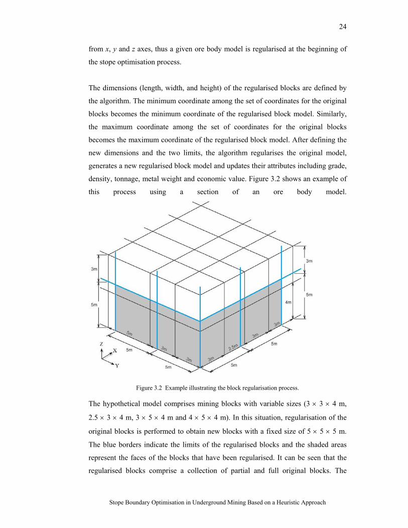
density, tonnage, metal weight and economic value. Figure 3.2 shows an example of
this process using a section of an ore body model.
Figure 3.2 Example illustrating the block regularisation process.
The hypothetical model comprises mining blocks with variable sizes (3 3 4 m,
2.5 3 4 m, 3 5 4 m and 4 5 4 m). In this situation, regularisation of the
original blocks is performed to obtain new blocks with a fixed size of 5 5 5 m.
The blue borders indicate the limits of the regularised blocks and the shaded areas
represent the faces of the blocks that have been regularised. It can be seen that the
regularised blocks comprise a collection of partial and full original blocks. The
25
Stope Boundary Optimisation in Underground Mining Based on a Heuristic Approach
algorithm updates the mining parameters for a regularised block based on the
attributes of the partial or complete original blocks, which are inside a regularised
block. The following notations are defined to explain the mathematical formulations
of the block attributes.
%orgrampertonne
$
%orgrampertonne
Equations 1 8 represent formulations of the block attributes, where ∈
and is a set of blocks that overlap with a block .
1
2
′
3
⁄ 4
26
Stope Boundary Optimisation in Underground Mining Based on a Heuristic Approach
Equations 5 and 6 represent and formulations for metals where the grade
is defined in %.
10′
5
10 100
6
Equations 7 and 8 represent and formulations for metals where the grade
is defined in grams/tonne.
′
7
⁄
8
3.2 CONVERTING THE GEOLOGICAL MODEL INTO AN ECONOMIC
MODEL
In the second stage of the process, the algorithm calculates the block economic
values to translate the regularised resource model into an economic model. The
following notations are used to explain the mathematical formulations of the block
economic values. The C# object-oriented source code for this formulation has been
included in Subsection 1 in Appendix B.
$/ $/
$/
$/
$/
%
$
Equation (9) is used to calculate .
(9)
3.3 STOPE GENERATION
Given the regularised economic model, the algorithm generates stopes in the third
stage of the process. It defines the stope size in terms of the number of blocks from
27
Stope Boundary Optimisation in Underground Mining Based on a Heuristic Approach
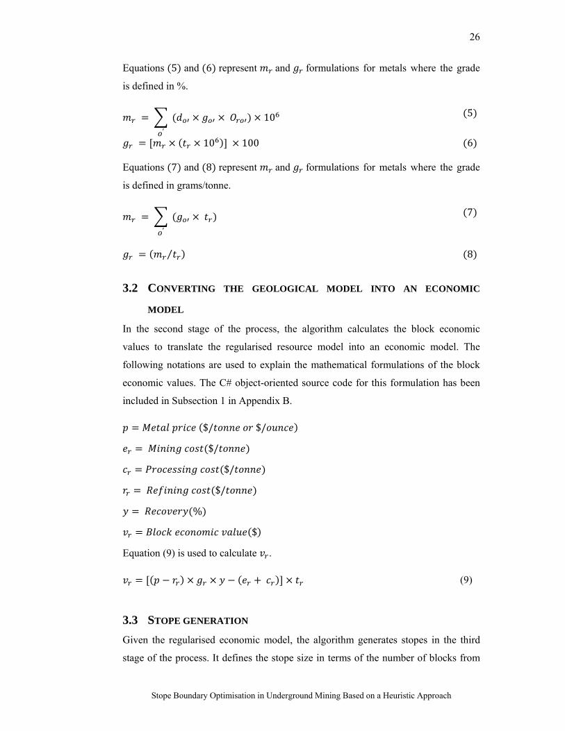
the x, y and z axes, and generates a set of possible stopes. Figure 3.3 shows an
example of a 2 3 2 stope size definition, i.e., two blocks along the x axis, three
blocks along the y axis and two blocks along the z axis, which are inside a block
model that has been regularised to a block size of 5 5 5 m.
Figure 3.3 Block model with a stope size of 2 3 2 blocks and a block size of 5 5 5 m.
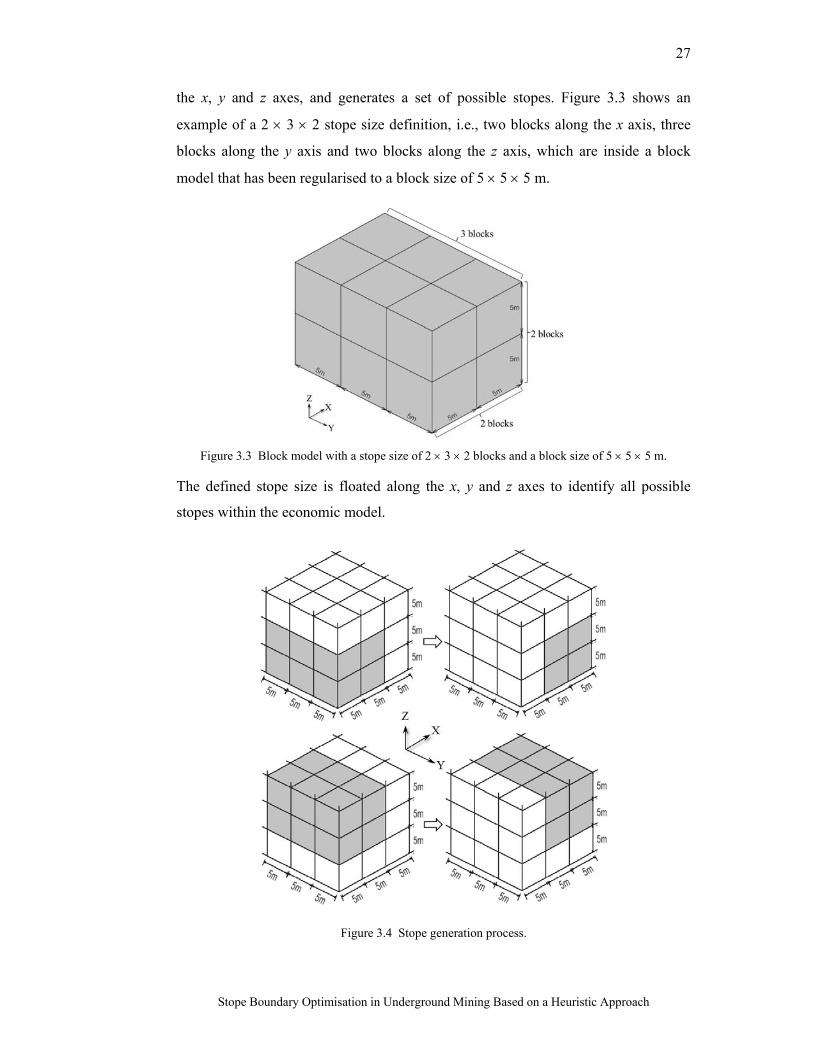
The defined stope size is floated along the x, y and z axes to identify all possible
stopes within the economic model.
Figure 3.4 Stope generation process.
28
Stope Boundary Optimisation in Underground Mining Based on a Heuristic Approach
Figure 3.4 illustrates an example of the stope generation process using a regularised
block model comprising of 27 mining blocks, i.e., three blocks along the x axis, three
blocks along the y axis and three blocks along the z axis. The stope size defined in
Figure 3.3 is floated along x, y and z axes and four possible stopes are generated
within this block model.
The following notations are used to explain the mathematical formulations for the
stope generating algorithm.
s= stope indicator
, , = location (x, y, z coordinates) of block
, , = location (x, y, z) of stope
, , = length (m), width (m), and height (m) of stope
= metal content or grade (% or grams/ tonne) of stope
= material density (tonnes/ m3) of stope
= metal weight (grams) of stope
= total weight (tonnes) of stope
= economic value ($) of stope
, , = number of mining blocks inside stope along the x, y, and z axes
, , = location (x, y, z coordinates) of the starting (origin) block of stope
, , = location (x, y, z coordinates) of the end (last) block of stope
, , = block identifier that facilitates stope generation
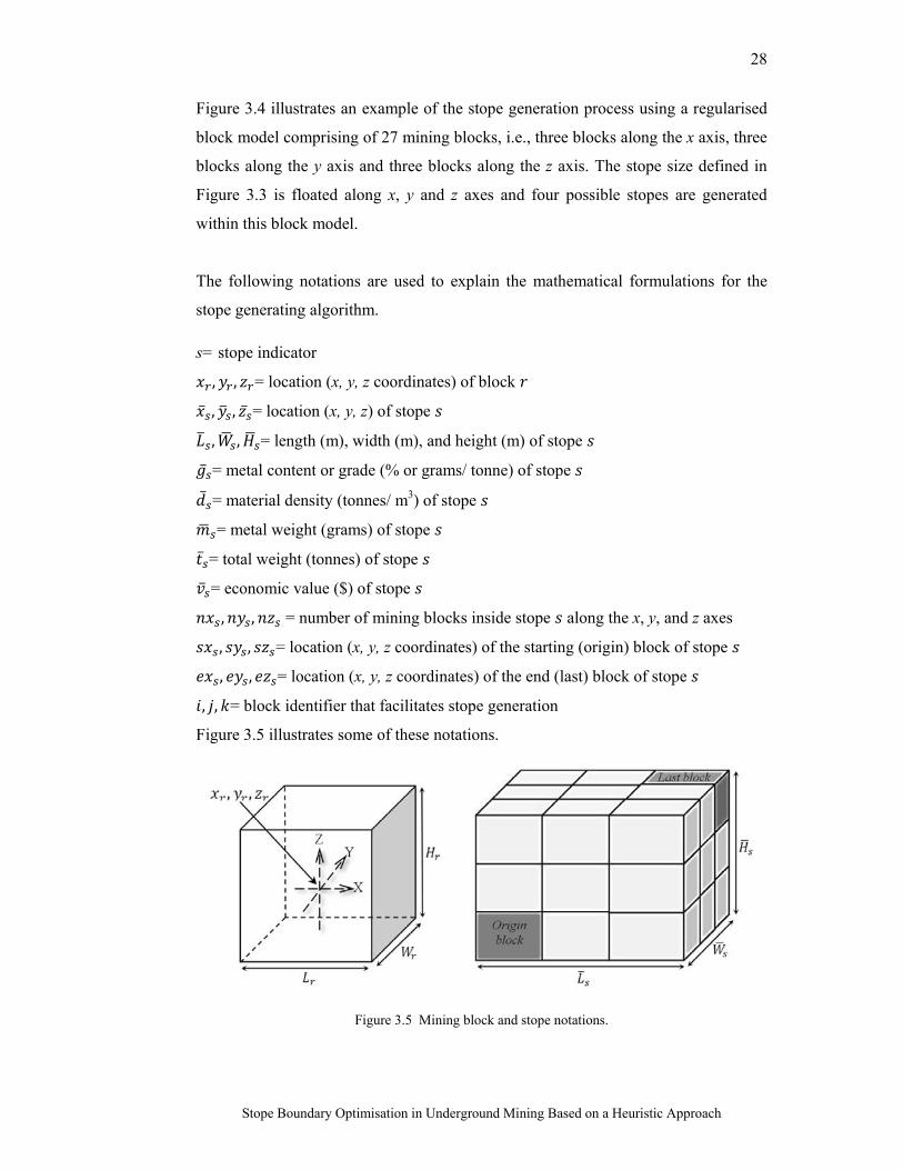
Figure 3.5 illustrates some of these notations.
Figure 3.5 Mining block and stope notations.
Stop
3.3.1 ST
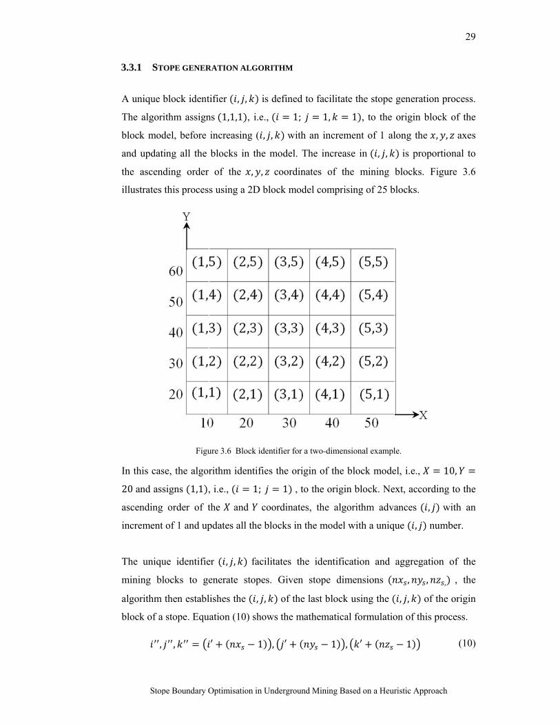
A unique
The algor
block mod
and updat
the ascen
illustrates
In this cas
20 and ass
ascending
increment
The uniqu
mining bl
algorithm
block of a
,
pe Boundary O
TOPE GENER
block ident
ithm assign
del, before
ting all the
ding order
this proces
Figu
se, the algor
signs 1,1 ,
order of t
t of 1 and up
ue identifie
locks to ge
then establ
a stope. Equ
,
Optimisation i
RATION ALG
tifier , ,
ns 1,1,1 , i
increasing
blocks in t
of the ,
s using a 2D
ure 3.6 Block
rithm identi
, i.e., 1
the and
pdates all th
er , , fa
enerate sto
lishes the
ation (10) s
′
in Undergroun
GORITHM
is defined
i.e., 1;
( , , with
the model.
, coordin
D block mo
k identifier for
ifies the ori
1; 1 , t
coordinate
he blocks in
facilitates th
pes. Given
, , of the
shows the m
1 , ′
nd Mining Ba
d to facilitat
1,
h an increm
The increas
nates of th
del compris
r a two-dimens
igin of the b
to the origin
es, the algo
the model w
he identific
n stope dim
e last block
mathematica
1 ,
ased on a Heur
e the stope
1 , to the
ment of 1 al
se in , ,
he mining
sing of 25 b
sional exampl
block mode
n block. Ne
orithm adva
with a uniq
cation and
mensions
using the
al formulatio
′
ristic Approac
generation
origin bloc
long the ,
is proport
blocks. Fig
blocks.
le.
el, i.e.,
ext, accordin
ances ,
que , num
aggregation
, ,
, , of th
on of this pr
1
29
ch
process.
ck of the
, axes
tional to
gure 3.6
10,
ng to the
with an
mber.
n of the
, , the
he origin
rocess.
(10)
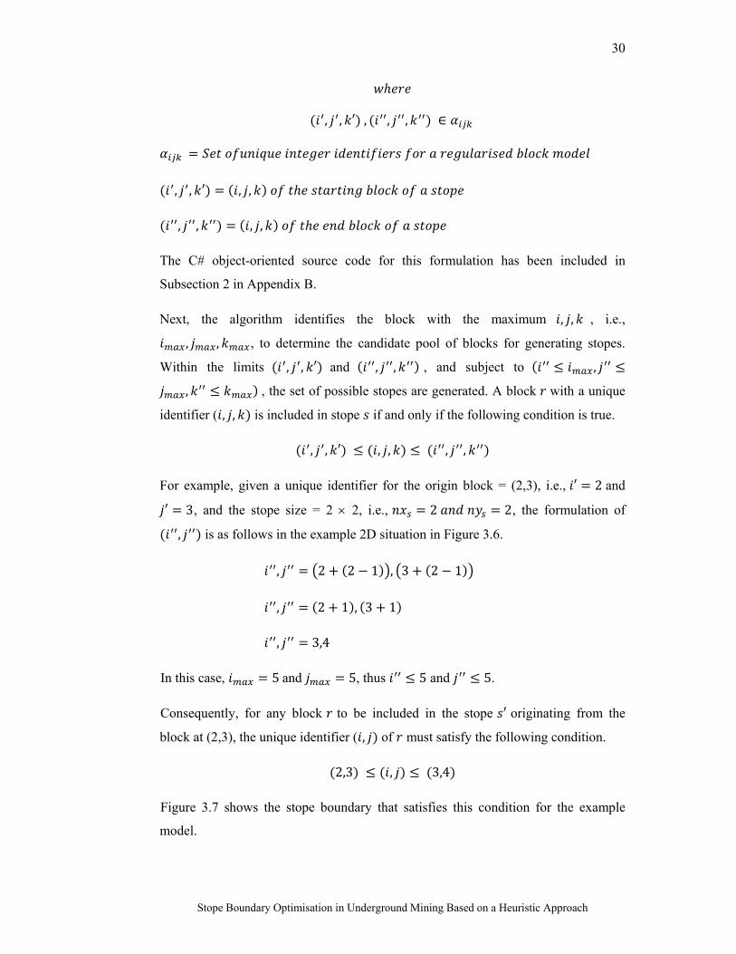
30
Stope Boundary Optimisation in Underground Mining Based on a Heuristic Approach
, , ′ , , , ∈
, , ′ , ,
, , , ,
The C# object-oriented source code for this formulation has been included in
Subsection 2 in Appendix B.
Next, the algorithm identifies the block with the maximum , , , i.e.,
, , , to determine the candidate pool of blocks for generating stopes.
Within the limits , , ′ and , , , and subject to ,
, , the set of possible stopes are generated. A block with a unique
identifier ( , , is included in stope if and only if the following condition is true.
, , ′ , , , ,
For example, given a unique identifier for the origin block = (2,3), i.e., ′ 2 and
′ 3, and the stope size = 2 2, i.e., 2 2, the formulation of
, is as follows in the example 2D situation in Figure 3.6.
, 2 2 1 , 3 2 1
, 2 1 , 3 1
, 3,4
In this case, 5and 5, thus 5 and 5.
Consequently, for any block to be included in the stope ′ originating from the
block at (2,3), the unique identifier ( , of must satisfy the following condition.
2,3 , 3,4
Figure 3.7 shows the stope boundary that satisfies this condition for the example
model.
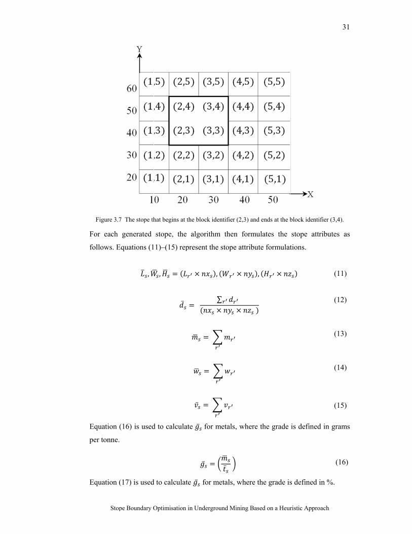
Stop
Figure 3.7
For each
follows. E
Equation (
per tonne.
Equation (
pe Boundary O
7 The stope th
generated
Equations (1
,
(16) is used
(17) is used
Optimisation i
hat begins at t
stope, the
1)–(15) rep
,
d to calculat
d to calculat
in Undergroun
the block iden
algorithm
present the s
,
∑
te for me
e for me
nd Mining Ba
ntifier (2,3) an
then form
stope attribu
etals, where
etals, where
ased on a Heur
nd ends at the b
mulates the
ute formulat
,
e the grade
the grade is
ristic Approac
block identifie
stope attrib
tions.
is defined i
s defined in
31
ch
er (3,4).
butes as
(11)
(12)
(13)
(14)
(15)
in grams
(16)
n %.
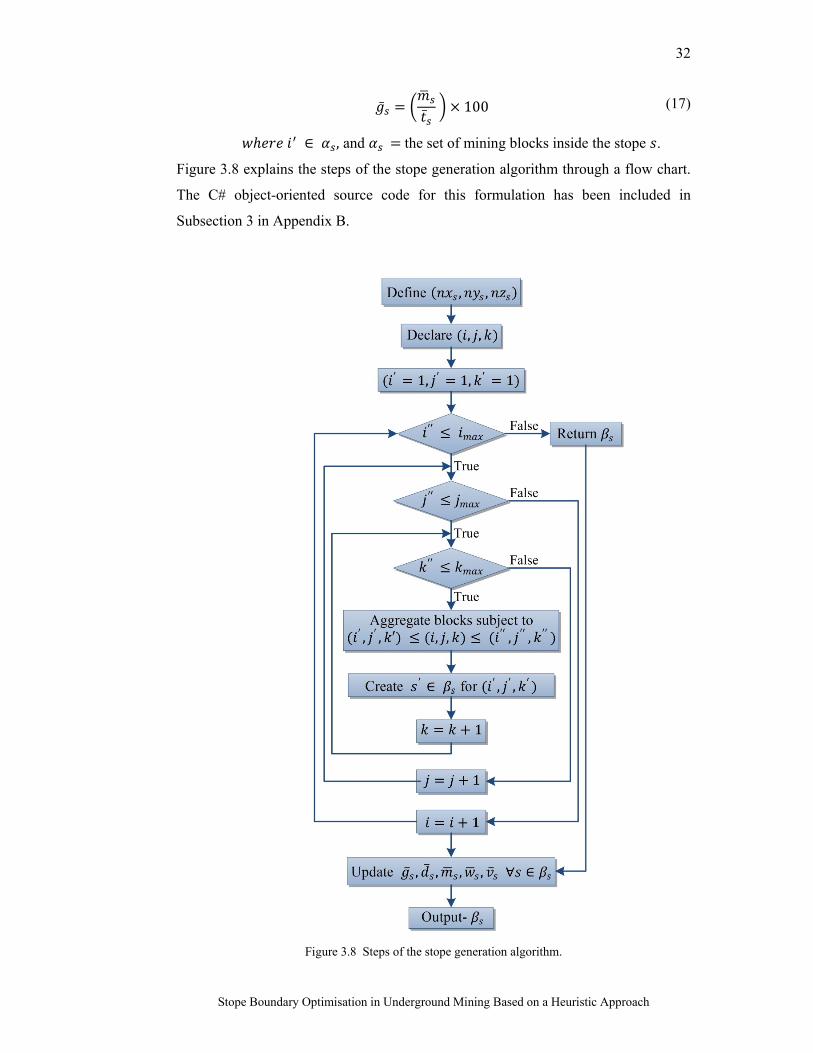
32
Stope Boundary Optimisation in Underground Mining Based on a Heuristic Approach
100 (17)
∈ , and the set of mining blocks inside the stope .
Figure 3.8 explains the steps of the stope generation algorithm through a flow chart.
The C# object-oriented source code for this formulation has been included in
Subsection 3 in Appendix B.
Figure 3.8 Steps of the stope generation algorithm.
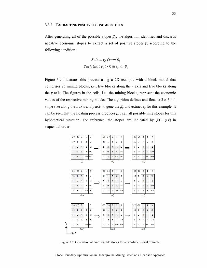
33
Stope Boundary Optimisation in Underground Mining Based on a Heuristic Approach
3.3.2 EXTRACTING POSITIVE ECONOMIC STOPES
After generating all of the possible stopes , the algorithm identifies and discards
negative economic stopes to extract a set of positive stopes according to the
following condition.
0 & ⊂
Figure 3.9 illustrates this process using a 2D example with a block model that
comprises 25 mining blocks, i.e., five blocks along the x axis and five blocks along
the y axis. The figures in the cells, i.e., the mining blocks, represent the economic
values of the respective mining blocks. The algorithm defines and floats a 3 3 1
stope size along the x axis and y axis to generate and extract for this example. It
can be seen that the floating process produces , i.e., all possible nine stopes for this
hypothetical situation. For reference, the stopes are indicated by in
sequential order.
Figure 3.9 Generation of nine possible stopes for a two-dimensional example.
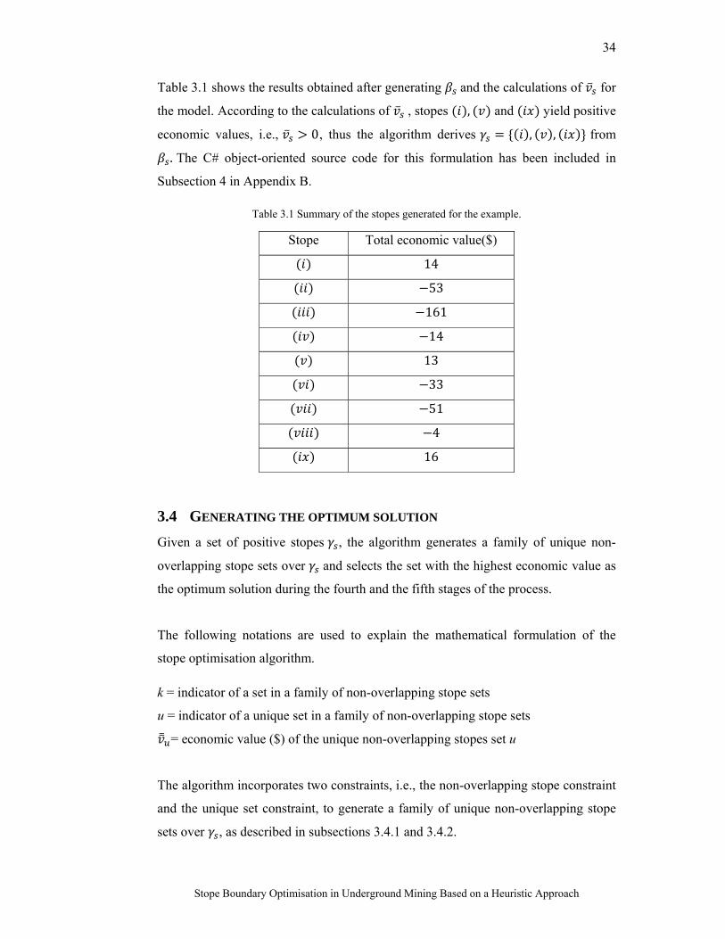
34
Stope Boundary Optimisation in Underground Mining Based on a Heuristic Approach
Table 3.1 shows the results obtained after generating and the calculations of for
the model. According to the calculations of , stopes , and yield positive
economic values, i.e., 0, thus the algorithm derives , , from
. The C# object-oriented source code for this formulation has been included in
Subsection 4 in Appendix B.
Table 3.1 Summary of the stopes generated for the example.
Stope Total economic value($)
14
53
161
14
13
33
51
4
16
3.4 GENERATING THE OPTIMUM SOLUTION
Given a set of positive stopes , the algorithm generates a family of unique non-
overlapping stope sets over and selects the set with the highest economic value as
the optimum solution during the fourth and the fifth stages of the process.
The following notations are used to explain the mathematical formulation of the
stope optimisation algorithm.
k = indicator of a set in a family of non-overlapping stope sets
u = indicator of a unique set in a family of non-overlapping stope sets
= economic value ($) of the unique non-overlapping stopes set u
The algorithm incorporates two constraints, i.e., the non-overlapping stope constraint
and the unique set constraint, to generate a family of unique non-overlapping stope
sets over , as described in subsections 3.4.1 and 3.4.2.
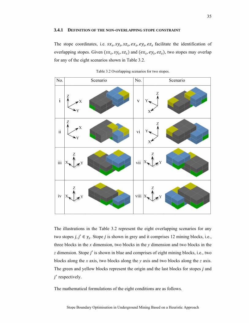
Stop
3.4.1 DE
The stope
overlappin
for any of
No.
i
ii
iii
iv
The illustr
two stopes
three bloc
z dimensio
blocks alo
The green
respecti
The mathe
Z
Z
X
X
pe Boundary O
EFINITION O
e coordinate
ng stopes. G
f the eight sc
S
rations in th
s , ′ ∈ . S
ks in the x
on. Stope ′
ong the x ax
n and yellow
ively.
ematical for
X
Y
X
Y
Z
Y
Z
Y
Optimisation i
OF THE NON
es, i.e. ,
Given ,
cenarios sho
Table 3.2 O
Scenario
he Table 3
Stope is sh
dimension,
is shown in
xis, two blo
w blocks rep
rmulations o
in Undergroun
N-OVERLAPP
, , ,
, an
own in Tabl
Overlapping sc
.2 represent
hown in gre
two blocks
n blue and c
cks along th
present the
of the eight
nd Mining Ba
PING STOPE
, ,
nd ,
le 3.2.
cenarios for tw
No.
v
vi
vii
viii
t the eight
ey and it co
s in the y dim
comprises o
he y axis an
origin and t
conditions
X
Y
X
Y
Z
X
Z
X
ased on a Heur
E CONSTRAIN
facilitate th
, , two
wo stopes.
Sce
overlapping
mprises 12
mension an
of eight min
nd two bloc
the last bloc
are as follo
Z
Z
Y
Y
ristic Approac
NT
he identific
stopes may
enario
g scenarios
mining blo
nd two block
ing blocks,
cks along th
cks for stop
ows.
35
ch
cation of
y overlap
for any
ocks, i.e.,
ks in the
i.e., two
he z axis.
pes and
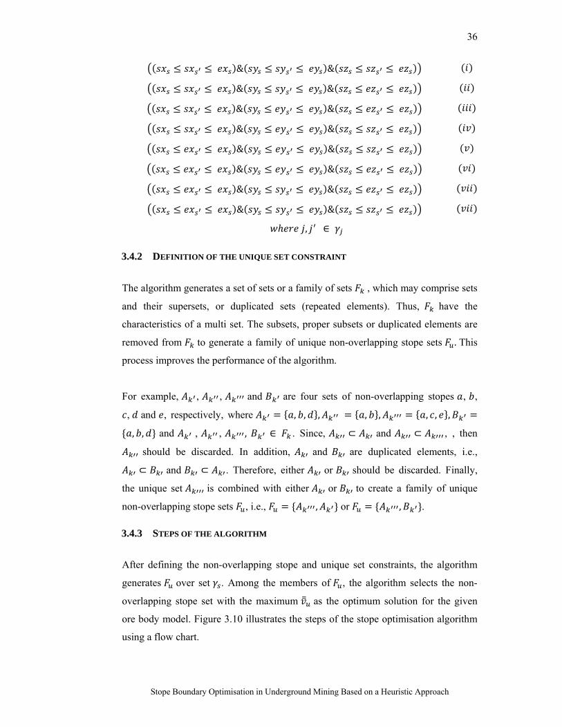
36
Stope Boundary Optimisation in Underground Mining Based on a Heuristic Approach
& &
& &
& &
& &
& &
& &
& &
& &
, ∈
3.4.2 DEFINITION OF THE UNIQUE SET CONSTRAINT
The algorithm generates a set of sets or a family of sets , which may comprise sets
and their supersets, or duplicated sets (repeated elements). Thus, have the
characteristics of a multi set. The subsets, proper subsets or duplicated elements are
removed from to generate a family of unique non-overlapping stope sets . This
process improves the performance of the algorithm.
For example, , , and are four sets of non-overlapping stopes , ,
, and , respectively, where , , , , , , , ,
, , and , , , ∈ . Since, ⊂ and ⊂ , , then
should be discarded. In addition, and are duplicated elements, i.e.,
⊂ and ⊂ . Therefore, either or should be discarded. Finally,
the unique set is combined with either or to create a family of unique
non-overlapping stope sets , i.e., , or , .
3.4.3 STEPS OF THE ALGORITHM
After defining the non-overlapping stope and unique set constraints, the algorithm
generates over set . Among the members of , the algorithm selects the non-
overlapping stope set with the maximum as the optimum solution for the given
ore body model. Figure 3.10 illustrates the steps of the stope optimisation algorithm
using a flow chart.
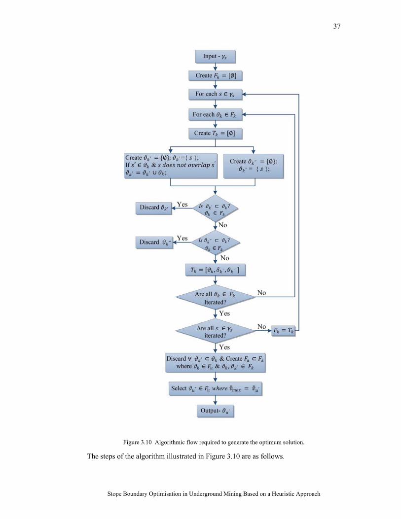
37
Stope Boundary Optimisation in Underground Mining Based on a Heuristic Approach
Figure 3.10 Algorithmic flow required to generate the optimum solution.
The steps of the algorithm illustrated in Figure 3.10 are as follows.
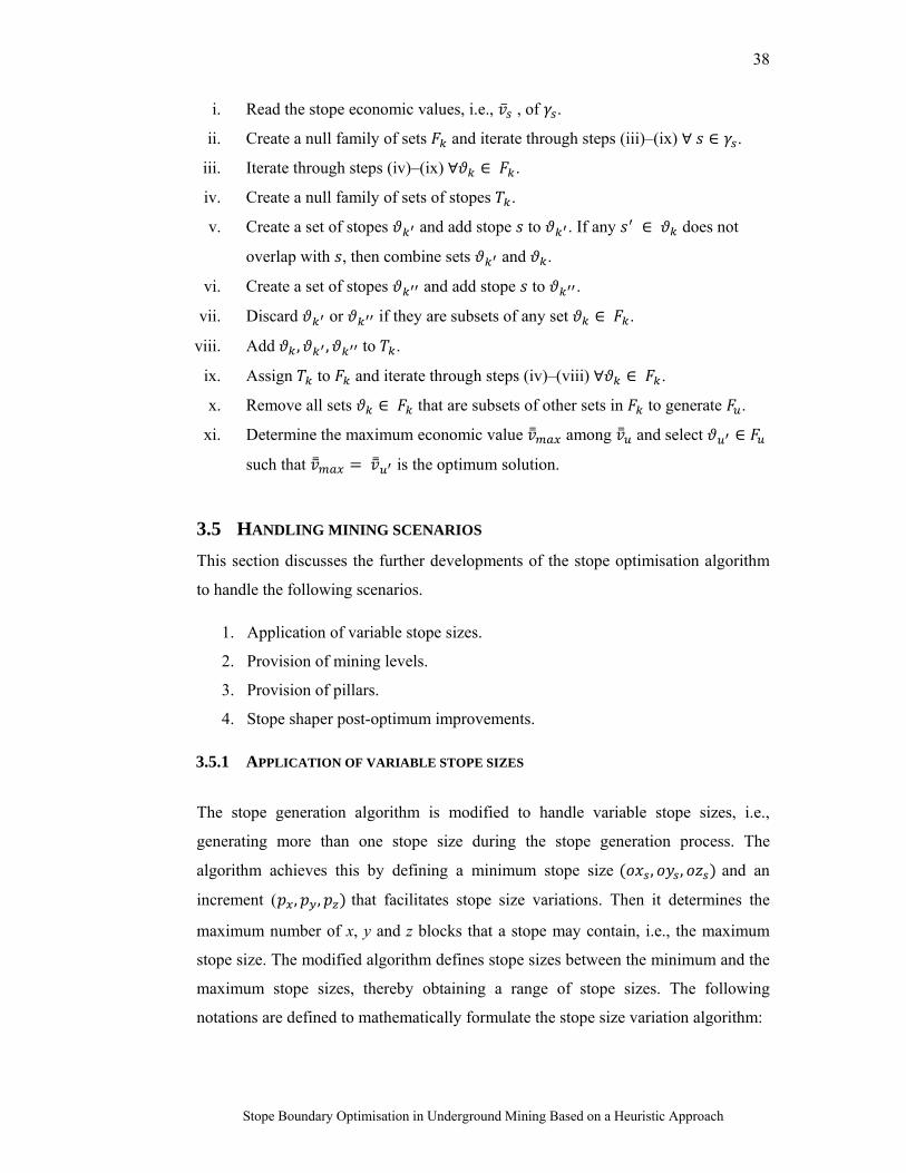
38
Stope Boundary Optimisation in Underground Mining Based on a Heuristic Approach
i. Read the stope economic values, i.e., , of .
ii. Create a null family of sets and iterate through steps (iii)–(ix) ∀ ∈ .
iii. Iterate through steps (iv)–(ix) ∀ ∈ .
iv. Create a null family of sets of stopes .
v. Create a set of stopes and add stope to . If any ∈ does not
overlap with , then combine sets and .
vi. Create a set of stopes and add stope to .
vii. Discard or if they are subsets of any set ∈ .
viii. Add , , to .
ix. Assign to and iterate through steps (iv)–(viii) ∀ ∈ .
x. Remove all sets ∈ that are subsets of other sets in to generate .
xi. Determine the maximum economic value among and select ∈
such that is the optimum solution.
3.5 HANDLING MINING SCENARIOS
This section discusses the further developments of the stope optimisation algorithm
to handle the following scenarios.
1. Application of variable stope sizes.
2. Provision of mining levels.
3. Provision of pillars.
4. Stope shaper post-optimum improvements.
3.5.1 APPLICATION OF VARIABLE STOPE SIZES
The stope generation algorithm is modified to handle variable stope sizes, i.e.,
generating more than one stope size during the stope generation process. The
algorithm achieves this by defining a minimum stope size , , and an
increment ( , , that facilitates stope size variations. Then it determines the
maximum number of x, y and z blocks that a stope may contain, i.e., the maximum
stope size. The modified algorithm defines stope sizes between the minimum and the
maximum stope sizes, thereby obtaining a range of stope sizes. The following
notations are defined to mathematically formulate the stope size variation algorithm:
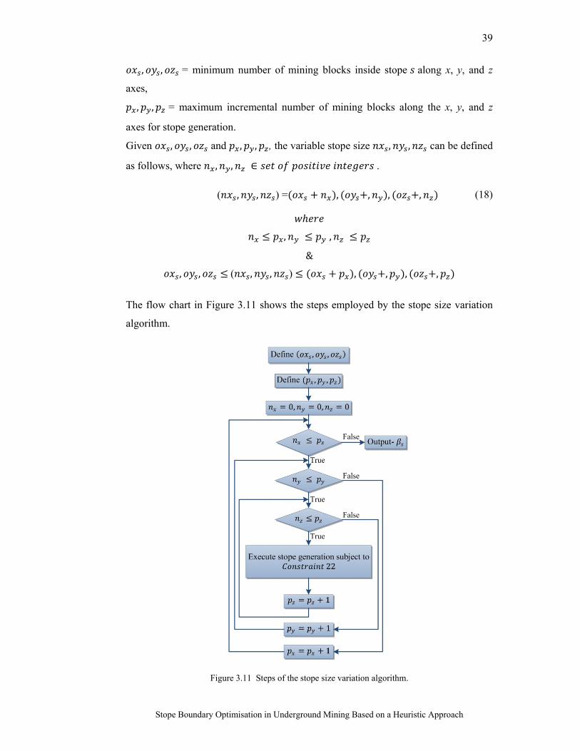
39
Stope Boundary Optimisation in Underground Mining Based on a Heuristic Approach
, , = minimum number of mining blocks inside stope along x, y, and z
axes,
, , = maximum incremental number of mining blocks along the x, y, and z
axes for stope generation.
Given , , and , , , the variable stope size , , can be defined
as follows, where , , ∈ .
( , , ) = , , , , (18)
, ,
&
, , ( , , ) , , , ,
The flow chart in Figure 3.11 shows the steps employed by the stope size variation
algorithm.
Figure 3.11 Steps of the stope size variation algorithm.
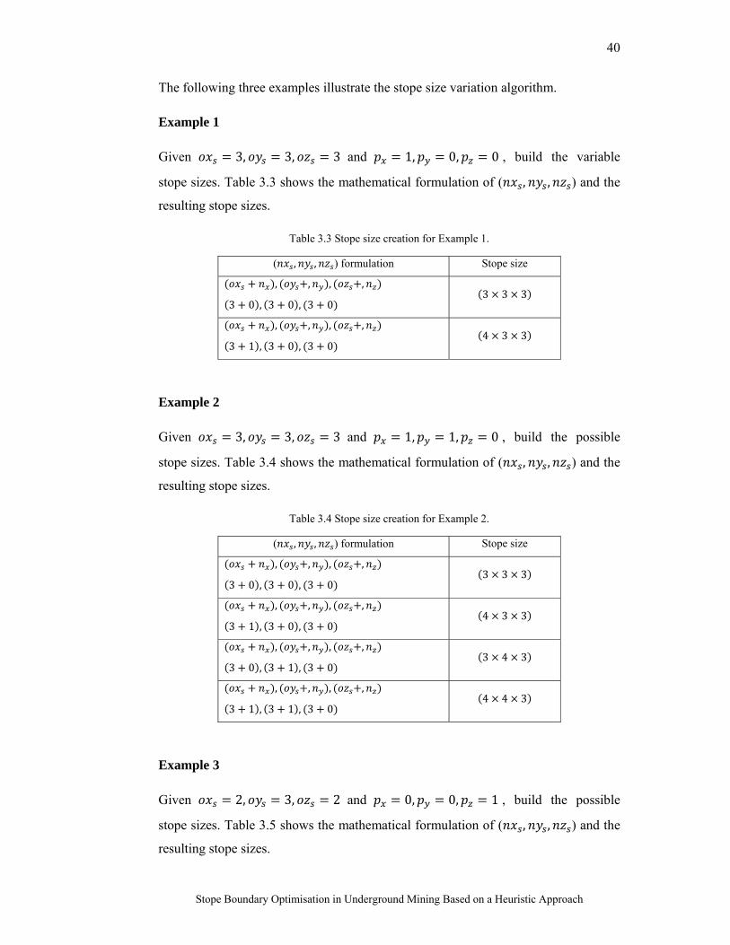
40
Stope Boundary Optimisation in Underground Mining Based on a Heuristic Approach
The following three examples illustrate the stope size variation algorithm.
Example 1
Given 3, 3, 3 and 1, 0, 0 , build the variable
stope sizes. Table 3.3 shows the mathematical formulation of ( , , ) and the
resulting stope sizes.
Table 3.3 Stope size creation for Example 1.
( , , ) formulation Stope size
, , , ,
3 0 , 3 0 , 3 0 3 3 3
, , , ,
3 1 , 3 0 , 3 0 4 3 3
Example 2
Given 3, 3, 3 and 1, 1, 0 , build the possible
stope sizes. Table 3.4 shows the mathematical formulation of ( , , ) and the
resulting stope sizes.
Table 3.4 Stope size creation for Example 2.
( , , ) formulation Stope size
, , , ,
3 0 , 3 0 , 3 0 3 3 3
, , , ,
3 1 , 3 0 , 3 0 4 3 3
, , , ,
3 0 , 3 1 , 3 0 3 4 3
, , , ,
3 1 , 3 1 , 3 0 4 4 3
Example 3
Given 2, 3, 2 and 0, 0, 1 , build the possible
stope sizes. Table 3.5 shows the mathematical formulation of ( , , ) and the
resulting stope sizes.
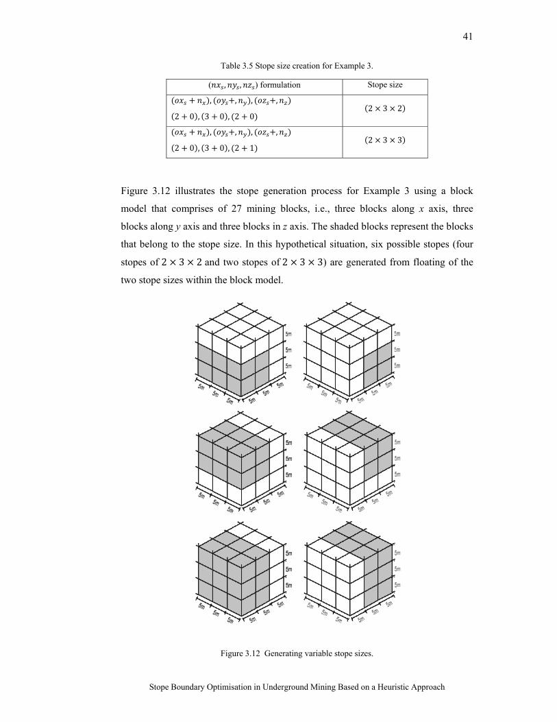
41
Stope Boundary Optimisation in Underground Mining Based on a Heuristic Approach
Table 3.5 Stope size creation for Example 3.
( , , ) formulation Stope size
, , , ,
2 0 , 3 0 , 2 0 2 3 2
, , , ,
2 0 , 3 0 , 2 1 2 3 3
Figure 3.12 illustrates the stope generation process for Example 3 using a block
model that comprises of 27 mining blocks, i.e., three blocks along x axis, three
blocks along y axis and three blocks in z axis. The shaded blocks represent the blocks
that belong to the stope size. In this hypothetical situation, six possible stopes (four
stopes of 2 3 2 and two stopes of2 3 3) are generated from floating of the
two stope sizes within the block model.
Figure 3.12 Generating variable stope sizes.
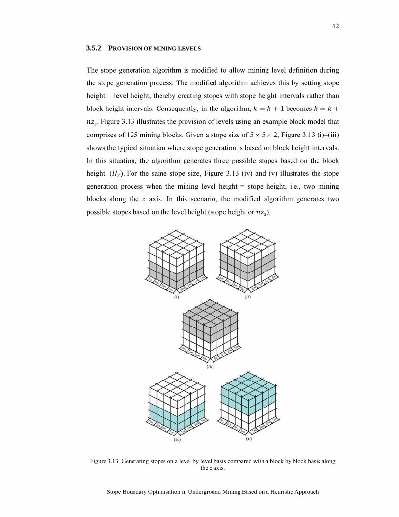
42
Stope Boundary Optimisation in Underground Mining Based on a Heuristic Approach
3.5.2 PROVISION OF MINING LEVELS
The stope generation algorithm is modified to allow mining level definition during
the stope generation process. The modified algorithm achieves this by setting stope
height = level height, thereby creating stopes with stope height intervals rather than
block height intervals. Consequently, in the algorithm, 1 becomes
. Figure 3.13 illustrates the provision of levels using an example block model that
comprises of 125 mining blocks. Given a stope size of 5 5 2, Figure 3.13 (i)–(iii)
shows the typical situation where stope generation is based on block height intervals.
In this situation, the algorithm generates three possible stopes based on the block
height, ( . For the same stope size, Figure 3.13 (iv) and (v) illustrates the stope
generation process when the mining level height = stope height, i.e., two mining
blocks along the z axis. In this scenario, the modified algorithm generates two
possible stopes based on the level height (stope height or ).
Figure 3.13 Generating stopes on a level by level basis compared with a block by block basis along the z axis.
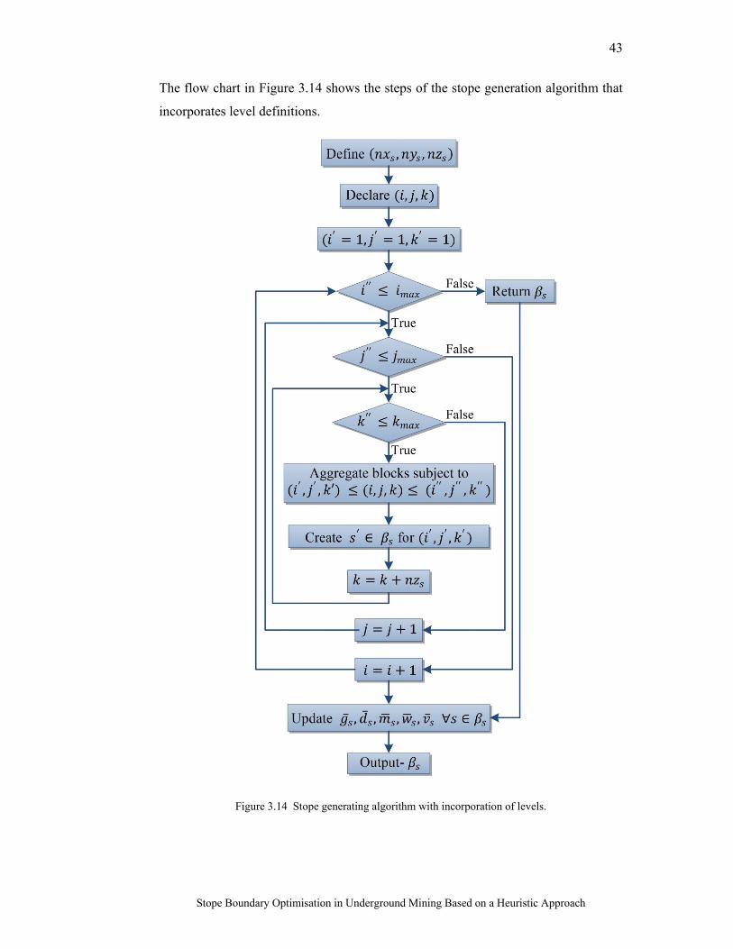
43
Stope Boundary Optimisation in Underground Mining Based on a Heuristic Approach
The flow chart in Figure 3.14 shows the steps of the stope generation algorithm that
incorporates level definitions.
Figure 3.14 Stope generating algorithm with incorporation of levels.
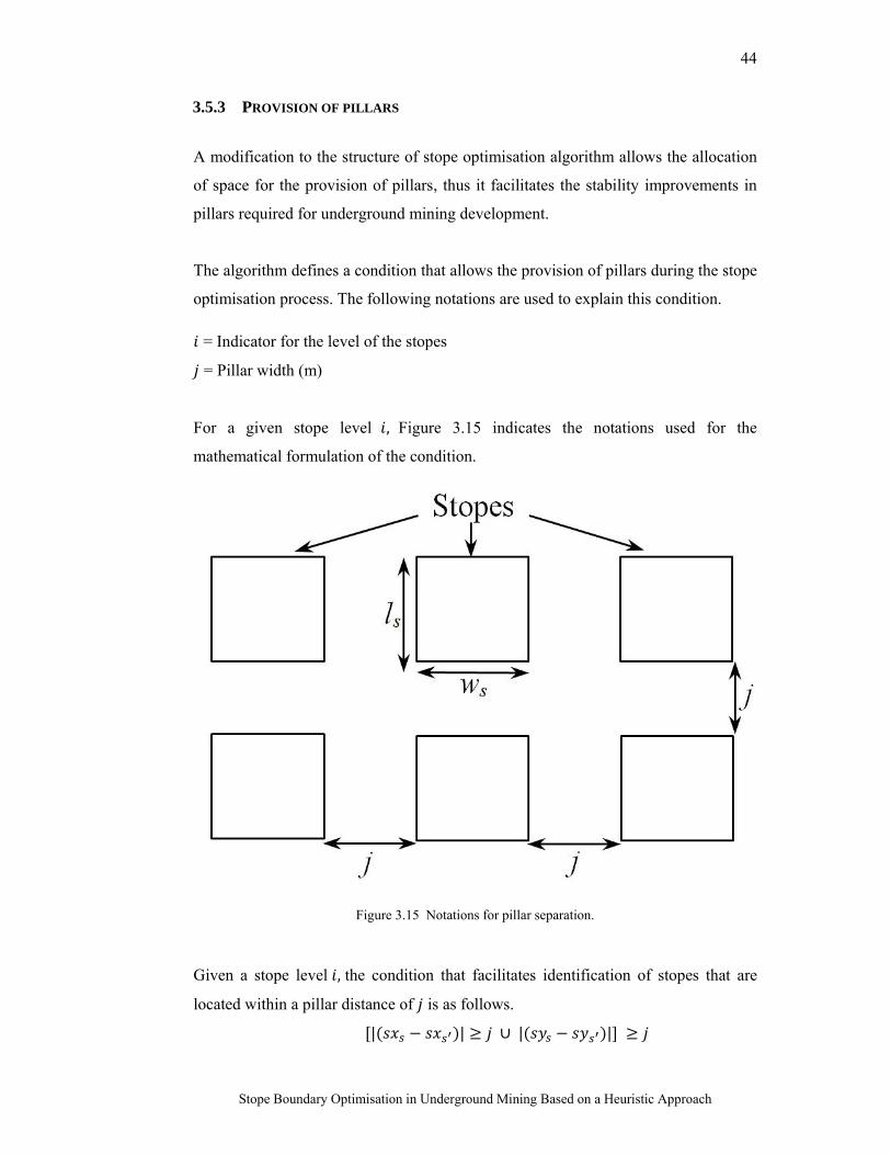
44
Stope Boundary Optimisation in Underground Mining Based on a Heuristic Approach
3.5.3 PROVISION OF PILLARS
A modification to the structure of stope optimisation algorithm allows the allocation
of space for the provision of pillars, thus it facilitates the stability improvements in
pillars required for underground mining development.
The algorithm defines a condition that allows the provision of pillars during the stope
optimisation process. The following notations are used to explain this condition.
= Indicator for the level of the stopes
= Pillar width (m)
For a given stope level , Figure 3.15 indicates the notations used for the
mathematical formulation of the condition.
Figure 3.15 Notations for pillar separation.
Given a stope level , the condition that facilitates identification of stopes that are
located within a pillar distance of is as follows.
| | ∪ | |
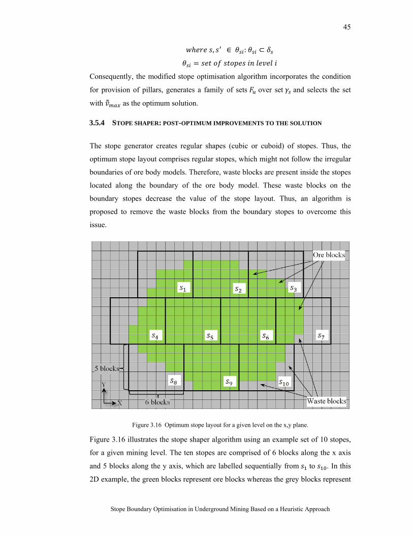
45
Stope Boundary Optimisation in Underground Mining Based on a Heuristic Approach
, ∈ : ⊂
Consequently, the modified stope optimisation algorithm incorporates the condition
for provision of pillars, generates a family of sets over set and selects the set
with as the optimum solution.
3.5.4 STOPE SHAPER: POST-OPTIMUM IMPROVEMENTS TO THE SOLUTION
The stope generator creates regular shapes (cubic or cuboid) of stopes. Thus, the
optimum stope layout comprises regular stopes, which might not follow the irregular
boundaries of ore body models. Therefore, waste blocks are present inside the stopes
located along the boundary of the ore body model. These waste blocks on the
boundary stopes decrease the value of the stope layout. Thus, an algorithm is
proposed to remove the waste blocks from the boundary stopes to overcome this
issue.
Figure 3.16 Optimum stope layout for a given level on the x,y plane.
Figure 3.16 illustrates the stope shaper algorithm using an example set of 10 stopes,
for a given mining level. The ten stopes are comprised of 6 blocks along the x axis
and 5 blocks along the y axis, which are labelled sequentially from to . In this
2D example, the green blocks represent ore blocks whereas the grey blocks represent
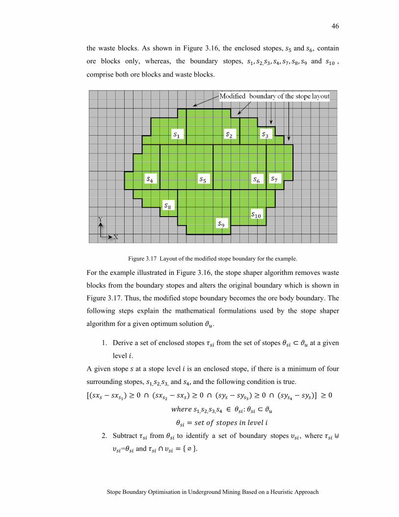
46
Stope Boundary Optimisation in Underground Mining Based on a Heuristic Approach
the waste blocks. As shown in Figure 3.16, the enclosed stopes, and , contain
ore blocks only, whereas, the boundary stopes, , , , , , , and ,
comprise both ore blocks and waste blocks.
Figure 3.17 Layout of the modified stope boundary for the example.
For the example illustrated in Figure 3.16, the stope shaper algorithm removes waste
blocks from the boundary stopes and alters the original boundary which is shown in
Figure 3.17. Thus, the modified stope boundary becomes the ore body boundary. The
following steps explain the mathematical formulations used by the stope shaper
algorithm for a given optimum solution .
1. Derive a set of enclosed stopes from the set of stopes ⊂ at a given
level .
A given stope at a stope level is an enclosed stope, if there is a minimum of four
surrounding stopes, , , , and , and the following condition is true.
0 ∩ 0 ∩ 0 ∩ 0
, , , ∈ : ⊂
2. Subtract from to identify a set of boundary stopes , where ⊎
= and ∩ ⌀ .
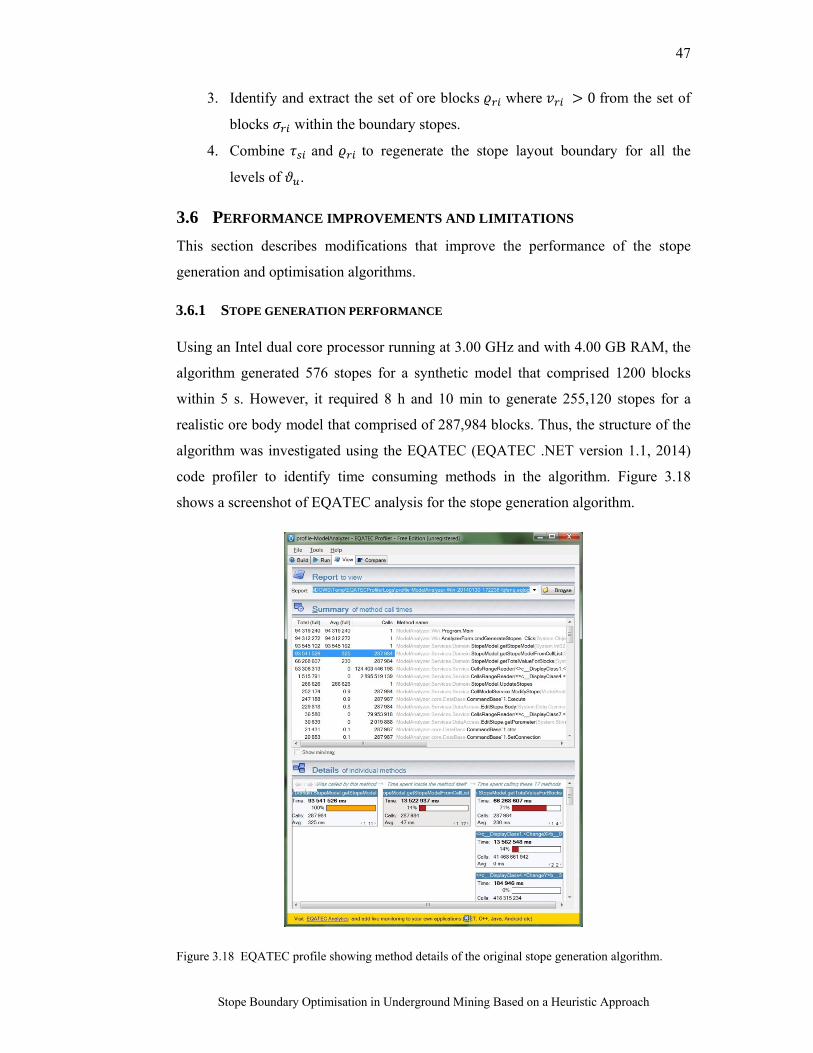
47
Stope Boundary Optimisation in Underground Mining Based on a Heuristic Approach
3. Identify and extract the set of ore blocks where 0 from the set of
blocks within the boundary stopes.
4. Combine and to regenerate the stope layout boundary for all the
levels of .
3.6 PERFORMANCE IMPROVEMENTS AND LIMITATIONS
This section describes modifications that improve the performance of the stope
generation and optimisation algorithms.
3.6.1 STOPE GENERATION PERFORMANCE Using an Intel dual core processor running at 3.00 GHz and with 4.00 GB RAM, the
algorithm generated 576 stopes for a synthetic model that comprised 1200 blocks
within 5 s. However, it required 8 h and 10 min to generate 255,120 stopes for a
realistic ore body model that comprised of 287,984 blocks. Thus, the structure of the
algorithm was investigated using the EQATEC (EQATEC .NET version 1.1, 2014)
code profiler to identify time consuming methods in the algorithm. Figure 3.18
shows a screenshot of EQATEC analysis for the stope generation algorithm.
Figure 3.18 EQATEC profile showing method details of the original stope generation algorithm.
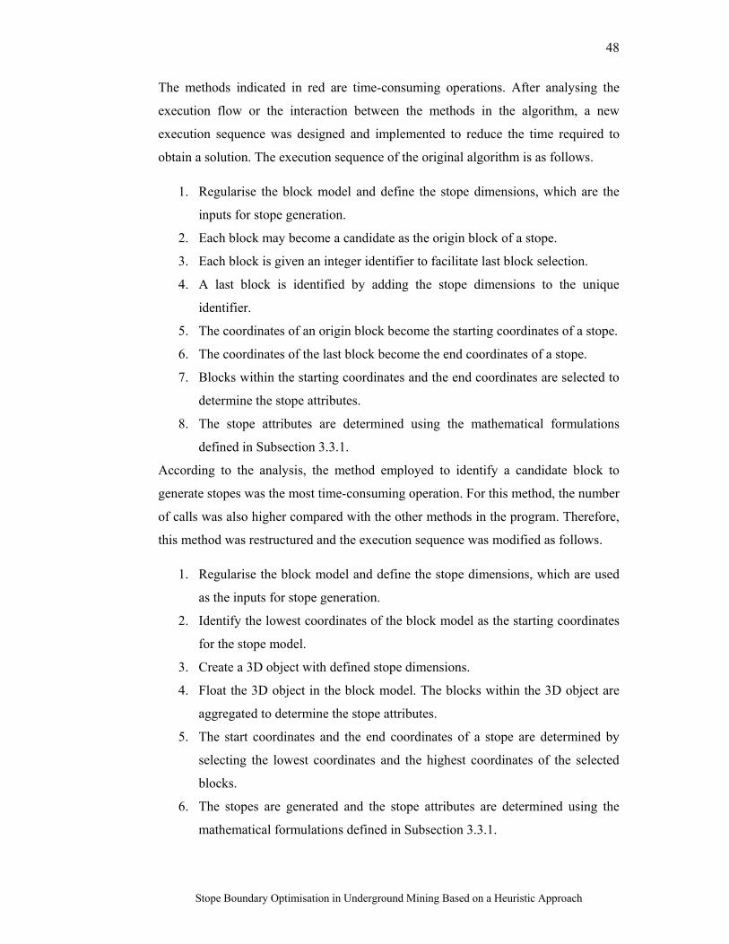
48
Stope Boundary Optimisation in Underground Mining Based on a Heuristic Approach
The methods indicated in red are time-consuming operations. After analysing the
execution flow or the interaction between the methods in the algorithm, a new
execution sequence was designed and implemented to reduce the time required to
obtain a solution. The execution sequence of the original algorithm is as follows.
1. Regularise the block model and define the stope dimensions, which are the
inputs for stope generation.
2. Each block may become a candidate as the origin block of a stope.
3. Each block is given an integer identifier to facilitate last block selection.
4. A last block is identified by adding the stope dimensions to the unique
identifier.
5. The coordinates of an origin block become the starting coordinates of a stope.
6. The coordinates of the last block become the end coordinates of a stope.
7. Blocks within the starting coordinates and the end coordinates are selected to
determine the stope attributes.
8. The stope attributes are determined using the mathematical formulations
defined in Subsection 3.3.1.
According to the analysis, the method employed to identify a candidate block to
generate stopes was the most time-consuming operation. For this method, the number
of calls was also higher compared with the other methods in the program. Therefore,
this method was restructured and the execution sequence was modified as follows.
1. Regularise the block model and define the stope dimensions, which are used
as the inputs for stope generation.
2. Identify the lowest coordinates of the block model as the starting coordinates
for the stope model.
3. Create a 3D object with defined stope dimensions.
4. Float the 3D object in the block model. The blocks within the 3D object are
aggregated to determine the stope attributes.
5. The start coordinates and the end coordinates of a stope are determined by
selecting the lowest coordinates and the highest coordinates of the selected
blocks.
6. The stopes are generated and the stope attributes are determined using the
mathematical formulations defined in Subsection 3.3.1.
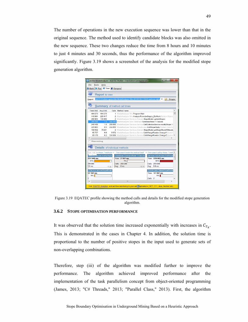
49
Stope Boundary Optimisation in Underground Mining Based on a Heuristic Approach
The number of operations in the new execution sequence was lower than that in the
original sequence. The method used to identify candidate blocks was also omitted in
the new sequence. These two changes reduce the time from 8 hours and 10 minutes
to just 4 minutes and 30 seconds, thus the performance of the algorithm improved
significantly. Figure 3.19 shows a screenshot of the analysis for the modified stope
generation algorithm.
Figure 3.19 EQATEC profile showing the method calls and details for the modified stope generation algorithm.
3.6.2 STOPE OPTIMISATION PERFORMANCE
It was observed that the solution time increased exponentially with increases in .
This is demonstrated in the cases in Chapter 4. In addition, the solution time is
proportional to the number of positive stopes in the input used to generate sets of
non-overlapping combinations.
Therefore, step (iii) of the algorithm was modified further to improve the
performance. The algorithm achieved improved performance after the
implementation of the task parallelism concept from object-oriented programming
(James, 2013; "C# Threads," 2013; "Parallel Class," 2013). First, the algorithm
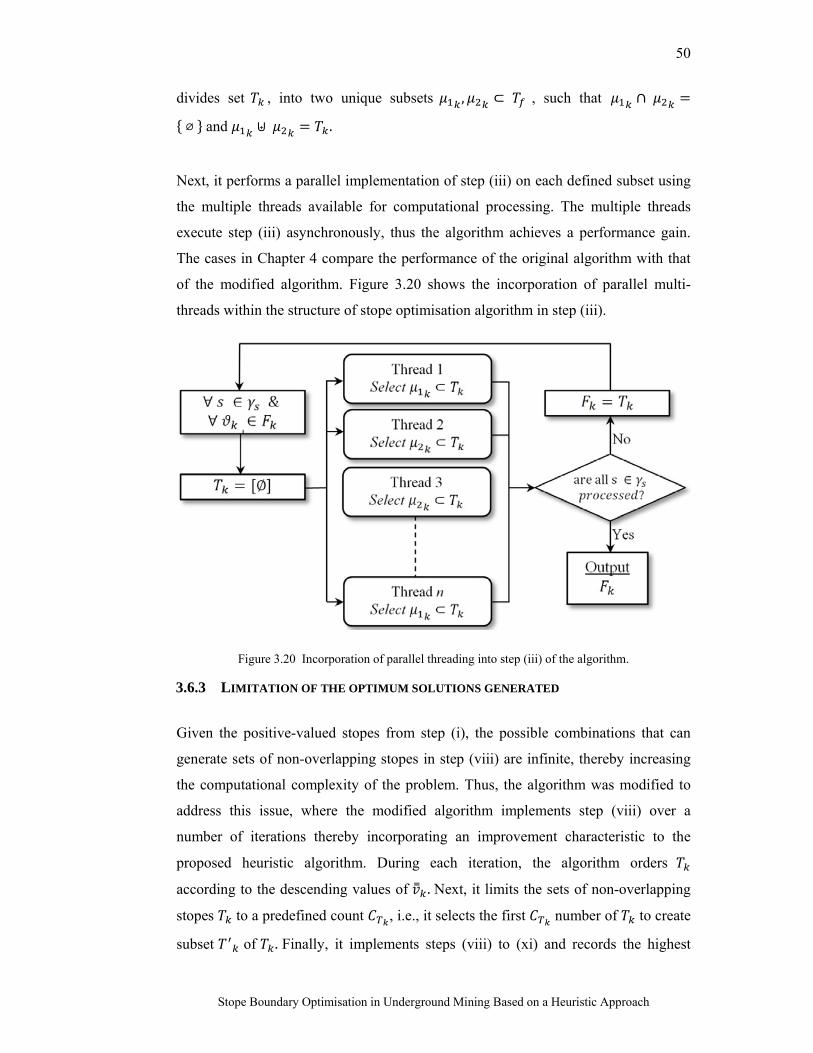
50
Stope Boundary Optimisation in Underground Mining Based on a Heuristic Approach
divides set , into two unique subsets , ⊂ , such that ∩
⌀ and ⊎ .
Next, it performs a parallel implementation of step (iii) on each defined subset using
the multiple threads available for computational processing. The multiple threads
execute step (iii) asynchronously, thus the algorithm achieves a performance gain.
The cases in Chapter 4 compare the performance of the original algorithm with that
of the modified algorithm. Figure 3.20 shows the incorporation of parallel multi-
threads within the structure of stope optimisation algorithm in step (iii).
Figure 3.20 Incorporation of parallel threading into step (iii) of the algorithm.
3.6.3 LIMITATION OF THE OPTIMUM SOLUTIONS GENERATED
Given the positive-valued stopes from step (i), the possible combinations that can
generate sets of non-overlapping stopes in step (viii) are infinite, thereby increasing
the computational complexity of the problem. Thus, the algorithm was modified to
address this issue, where the modified algorithm implements step (viii) over a
number of iterations thereby incorporating an improvement characteristic to the
proposed heuristic algorithm. During each iteration, the algorithm orders
according to the descending values of . Next, it limits the sets of non-overlapping
stopes to a predefined count , i.e., it selects the first number of to create
subset of . Finally, it implements steps (viii) to (xi) and records the highest
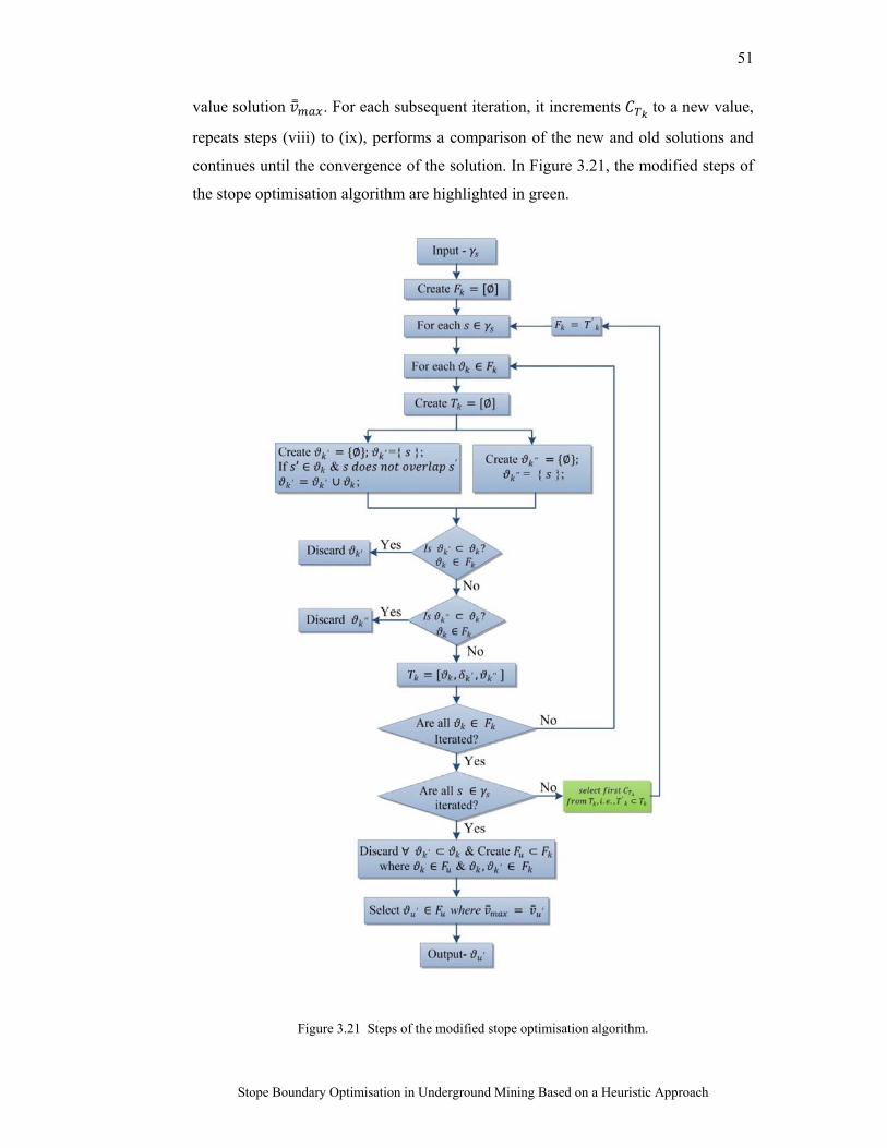
51
Stope Boundary Optimisation in Underground Mining Based on a Heuristic Approach
value solution . For each subsequent iteration, it increments to a new value,
repeats steps (viii) to (ix), performs a comparison of the new and old solutions and
continues until the convergence of the solution. In Figure 3.21, the modified steps of
the stope optimisation algorithm are highlighted in green.
Figure 3.21 Steps of the modified stope optimisation algorithm.
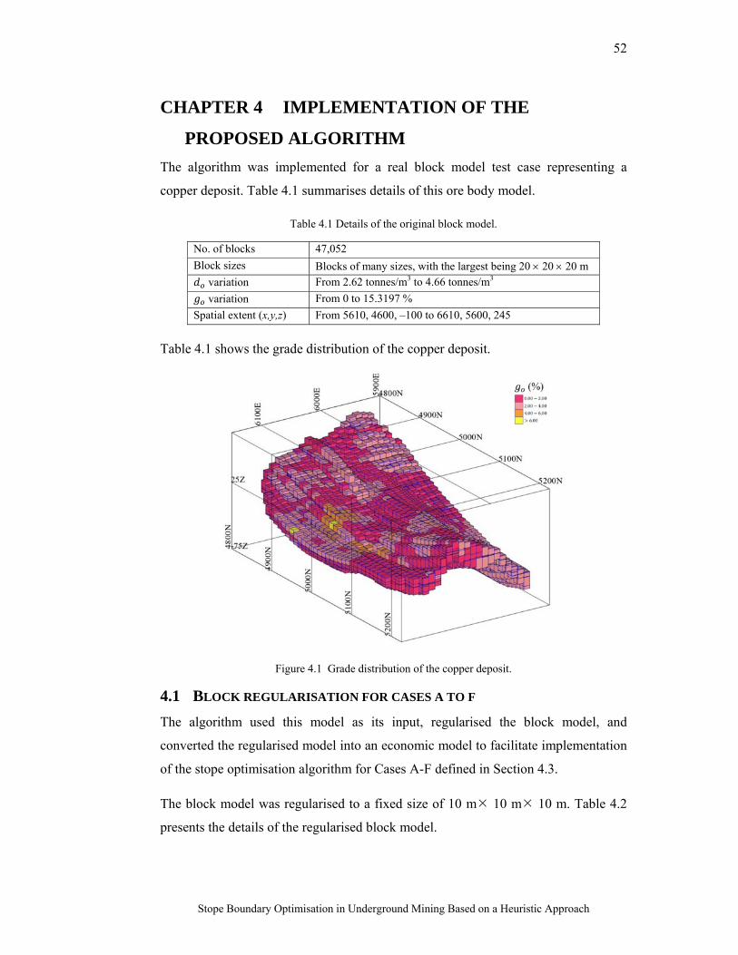
52
Stope Boundary Optimisation in Underground Mining Based on a Heuristic Approach
CHAPTER 4 IMPLEMENTATION OF THE
PROPOSED ALGORITHM
The algorithm was implemented for a real block model test case representing a
copper deposit. Table 4.1 summarises details of this ore body model.
Table 4.1 Details of the original block model.
No. of blocks 47,052
Block sizes Blocks of many sizes, with the largest being 20 20 20 m
variation From 2.62 tonnes/m3 to 4.66 tonnes/m3
variation From 0 to 15.3197 %
Spatial extent (x,y,z) From 5610, 4600, –100 to 6610, 5600, 245
Table 4.1 shows the grade distribution of the copper deposit.
Figure 4.1 Grade distribution of the copper deposit.
4.1 BLOCK REGULARISATION FOR CASES A TO F
The algorithm used this model as its input, regularised the block model, and
converted the regularised model into an economic model to facilitate implementation
of the stope optimisation algorithm for Cases A-F defined in Section 4.3.
The block model was regularised to a fixed size of 10 m 10 m 10 m. Table 4.2
presents the details of the regularised block model.
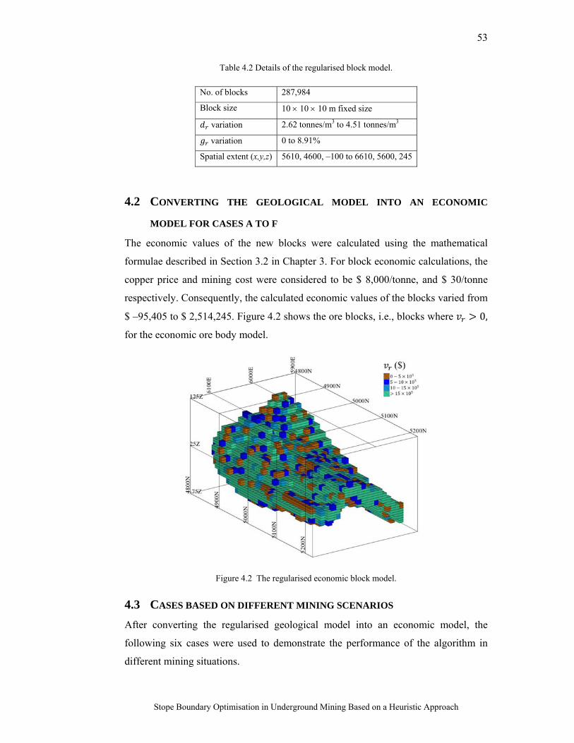
53
Stope Boundary Optimisation in Underground Mining Based on a Heuristic Approach
Table 4.2 Details of the regularised block model.
No. of blocks 287,984
Block size 10 10 10 m fixed size
variation 2.62 tonnes/m3 to 4.51 tonnes/m3
variation 0 to 8.91%
Spatial extent (x,y,z) 5610, 4600, –100 to 6610, 5600, 245
4.2 CONVERTING THE GEOLOGICAL MODEL INTO AN ECONOMIC
MODEL FOR CASES A TO F
The economic values of the new blocks were calculated using the mathematical
formulae described in Section 3.2 in Chapter 3. For block economic calculations, the
copper price and mining cost were considered to be $ 8,000/tonne, and $ 30/tonne
respectively. Consequently, the calculated economic values of the blocks varied from
$ –95,405 to $ 2,514,245. Figure 4.2 shows the ore blocks, i.e., blocks where 0,
for the economic ore body model.
Figure 4.2 The regularised economic block model.
4.3 CASES BASED ON DIFFERENT MINING SCENARIOS
After converting the regularised geological model into an economic model, the
following six cases were used to demonstrate the performance of the algorithm in
different mining situations.
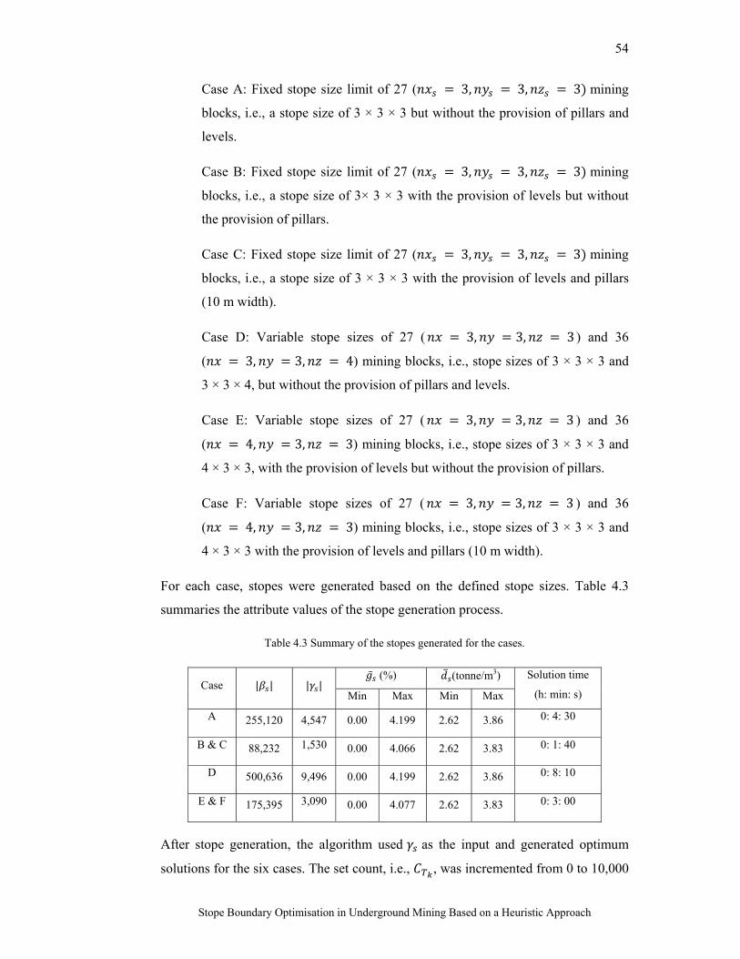
54
Stope Boundary Optimisation in Underground Mining Based on a Heuristic Approach
Case A: Fixed stope size limit of 27 ( 3, 3, 3 mining
blocks, i.e., a stope size of 3 × 3 × 3 but without the provision of pillars and
levels.
Case B: Fixed stope size limit of 27 ( 3, 3, 3 mining
blocks, i.e., a stope size of 3× 3 × 3 with the provision of levels but without
the provision of pillars.
Case C: Fixed stope size limit of 27 ( 3, 3, 3 mining
blocks, i.e., a stope size of 3 × 3 × 3 with the provision of levels and pillars
(10 m width).
Case D: Variable stope sizes of 27 ( 3, 3, 3 ) and 36
( 3, 3, 4) mining blocks, i.e., stope sizes of 3 × 3 × 3 and
3 × 3 × 4, but without the provision of pillars and levels.
Case E: Variable stope sizes of 27 ( 3, 3, 3 ) and 36
( 4, 3, 3) mining blocks, i.e., stope sizes of 3 × 3 × 3 and
4 × 3 × 3, with the provision of levels but without the provision of pillars.
Case F: Variable stope sizes of 27 ( 3, 3, 3 ) and 36
( 4, 3, 3) mining blocks, i.e., stope sizes of 3 × 3 × 3 and
4 × 3 × 3 with the provision of levels and pillars (10 m width).
For each case, stopes were generated based on the defined stope sizes. Table 4.3
summaries the attribute values of the stope generation process.
Table 4.3 Summary of the stopes generated for the cases.
Case | | | | (%) (tonne/m3) Solution time
(h: min: s) Min Max Min Max
A 255,120 4,547 0.00 4.199 2.62 3.86 0: 4: 30
B & C 88,232 1,530 0.00 4.066 2.62 3.83 0: 1: 40
D 500,636 9,496 0.00 4.199 2.62 3.86 0: 8: 10
E & F 175,395 3,090 0.00 4.077 2.62 3.83 0: 3: 00
After stope generation, the algorithm used as the input and generated optimum
solutions for the six cases. The set count, i.e., , was incremented from 0 to 10,000
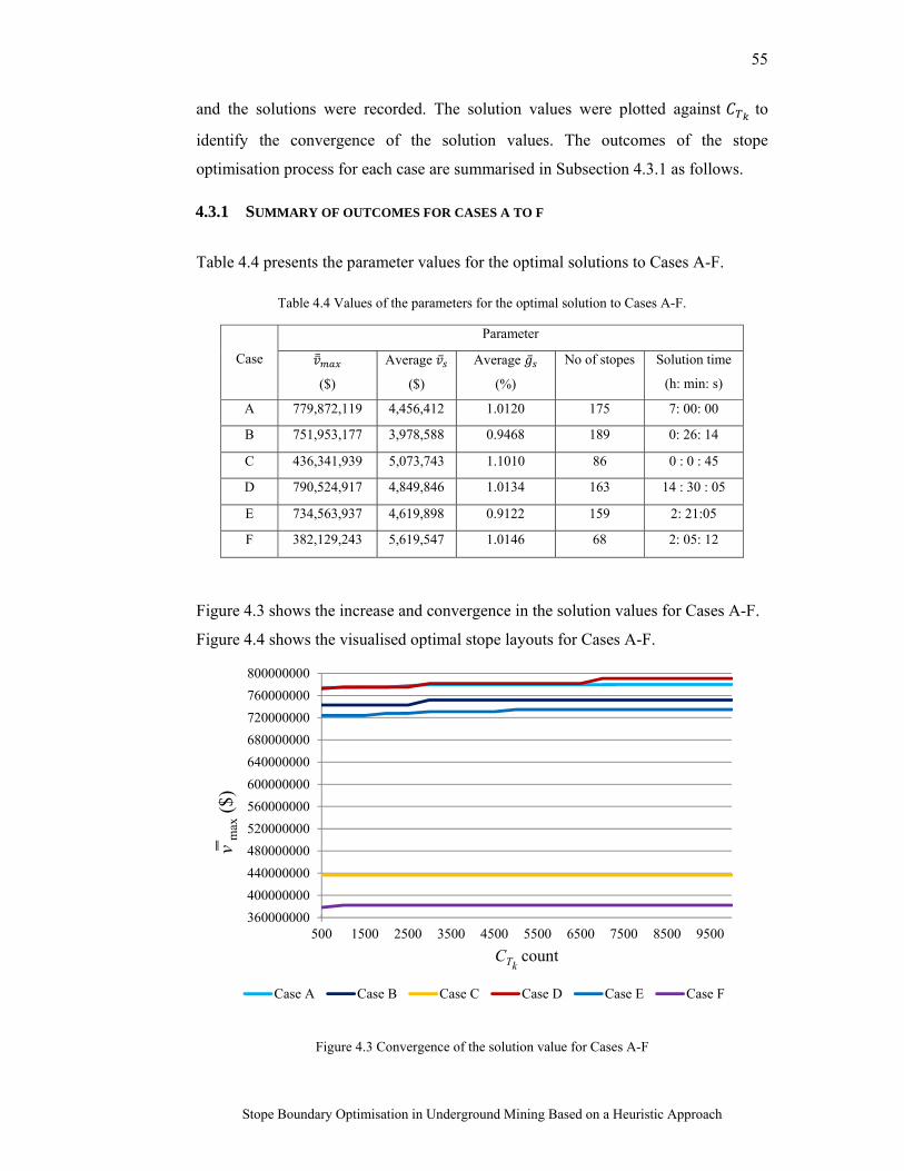
55
Stope Boundary Optimisation in Underground Mining Based on a Heuristic Approach
and the solutions were recorded. The solution values were plotted against to
identify the convergence of the solution values. The outcomes of the stope
optimisation process for each case are summarised in Subsection 4.3.1 as follows.
4.3.1 SUMMARY OF OUTCOMES FOR CASES A TO F
Table 4.4 presents the parameter values for the optimal solutions to Cases A-F.
Table 4.4 Values of the parameters for the optimal solution to Cases A-F.
Case
Parameter
($)
Average
($)
Average
(%)
No of stopes Solution time
(h: min: s)
A 779,872,119 4,456,412 1.0120 175 7: 00: 00
B 751,953,177 3,978,588 0.9468 189 0: 26: 14
C 436,341,939 5,073,743 1.1010 86 0 : 0 : 45
D 790,524,917 4,849,846 1.0134 163 14 : 30 : 05
E 734,563,937 4,619,898 0.9122 159 2: 21:05
F 382,129,243 5,619,547 1.0146 68 2: 05: 12
Figure 4.3 shows the increase and convergence in the solution values for Cases A-F.
Figure 4.4 shows the visualised optimal stope layouts for Cases A-F.
Figure 4.3 Convergence of the solution value for Cases A-F
360000000
400000000
440000000
480000000
520000000
560000000
600000000
640000000
680000000
720000000
760000000
800000000
500 1500 2500 3500 4500 5500 6500 7500 8500 9500
v m
ax($
)
CTkcount
Case A Case B Case C Case D Case E Case F
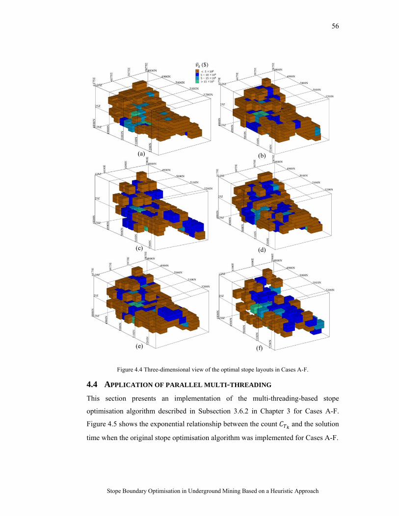
56
Stope Boundary Optimisation in Underground Mining Based on a Heuristic Approach
Figure 4.4 Three-dimensional view of the optimal stope layouts in Cases A-F.
4.4 APPLICATION OF PARALLEL MULTI-THREADING
This section presents an implementation of the multi-threading-based stope
optimisation algorithm described in Subsection 3.6.2 in Chapter 3 for Cases A-F.
Figure 4.5 shows the exponential relationship between the count and the solution
time when the original stope optimisation algorithm was implemented for Cases A-F.
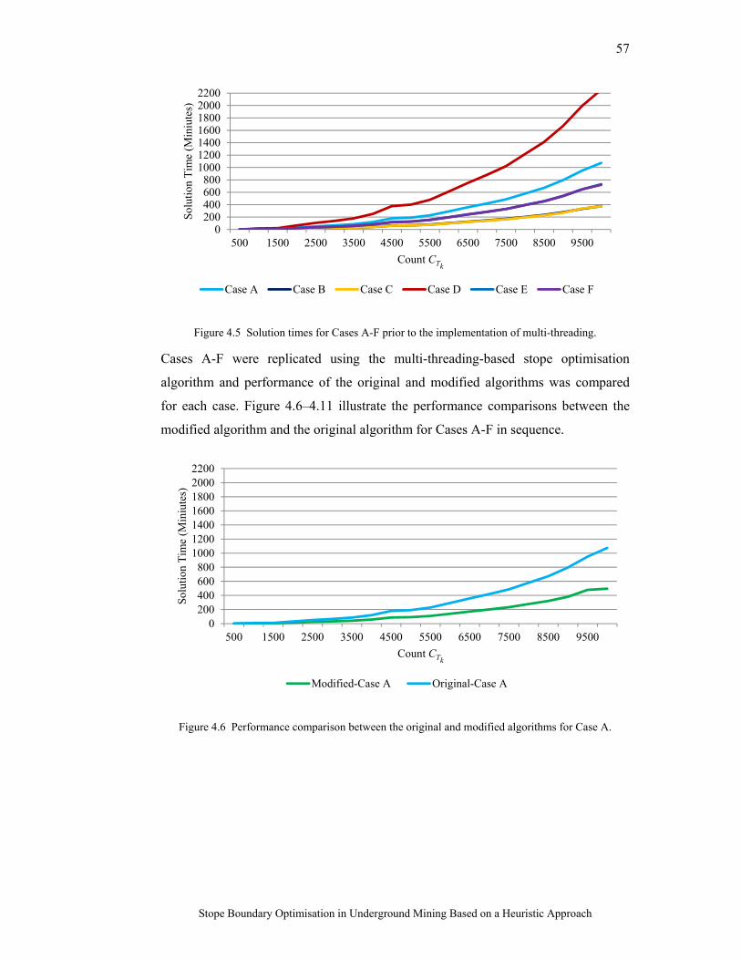
57
Stope Boundary Optimisation in Underground Mining Based on a Heuristic Approach
Figure 4.5 Solution times for Cases A-F prior to the implementation of multi-threading.
Cases A-F were replicated using the multi-threading-based stope optimisation
algorithm and performance of the original and modified algorithms was compared
for each case. Figure 4.6–4.11 illustrate the performance comparisons between the
modified algorithm and the original algorithm for Cases A-F in sequence.
Figure 4.6 Performance comparison between the original and modified algorithms for Case A.
0200400600800
1000120014001600180020002200
500 1500 2500 3500 4500 5500 6500 7500 8500 9500
Sol
utio
n T
ime
(Min
iute
s)
Count CTk
Case A Case B Case C Case D Case E Case F
0200400600800
1000120014001600180020002200
500 1500 2500 3500 4500 5500 6500 7500 8500 9500
Solu
tion
Tim
e (M
iniu
tes)
Count CTk
Modified-Case A Original-Case A
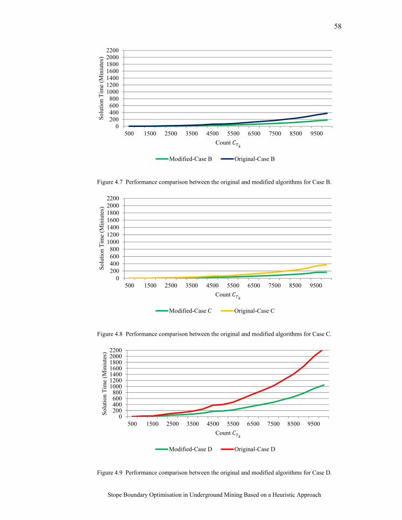
58
Stope Boundary Optimisation in Underground Mining Based on a Heuristic Approach
Figure 4.7 Performance comparison between the original and modified algorithms for Case B.
Figure 4.8 Performance comparison between the original and modified algorithms for Case C.
Figure 4.9 Performance comparison between the original and modified algorithms for Case D.
0200400600800
1000120014001600180020002200
500 1500 2500 3500 4500 5500 6500 7500 8500 9500
Sol
utio
n T
ime
(Min
iute
s)
Count
Modified-Case B Original-Case B
0200400600800
1000120014001600180020002200
500 1500 2500 3500 4500 5500 6500 7500 8500 9500
Sol
utio
n T
ime
(Min
iute
s)
Count
Modified-Case C Original-Case C
0200400600800
1000120014001600180020002200
500 1500 2500 3500 4500 5500 6500 7500 8500 9500
Sol
utio
n T
ime
(Min
iute
s)
Count
Modified-Case D Original-Case D
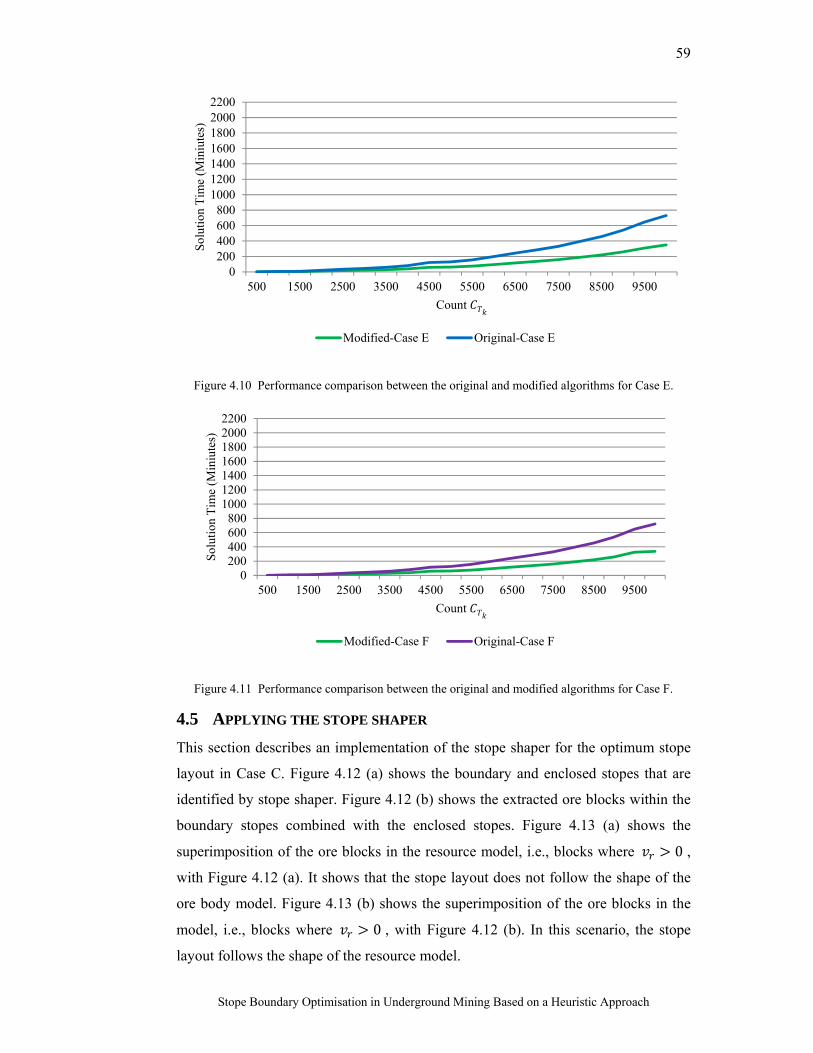
59
Stope Boundary Optimisation in Underground Mining Based on a Heuristic Approach
Figure 4.10 Performance comparison between the original and modified algorithms for Case E.
Figure 4.11 Performance comparison between the original and modified algorithms for Case F.
4.5 APPLYING THE STOPE SHAPER
This section describes an implementation of the stope shaper for the optimum stope
layout in Case C. Figure 4.12 (a) shows the boundary and enclosed stopes that are
identified by stope shaper. Figure 4.12 (b) shows the extracted ore blocks within the
boundary stopes combined with the enclosed stopes. Figure 4.13 (a) shows the
superimposition of the ore blocks in the resource model, i.e., blocks where 0 ,
with Figure 4.12 (a). It shows that the stope layout does not follow the shape of the
ore body model. Figure 4.13 (b) shows the superimposition of the ore blocks in the
model, i.e., blocks where 0 , with Figure 4.12 (b). In this scenario, the stope
layout follows the shape of the resource model.
0200400600800
1000120014001600180020002200
500 1500 2500 3500 4500 5500 6500 7500 8500 9500
Sol
utio
n T
ime
(Min
iute
s)
Count
Modified-Case E Original-Case E
0200400600800
1000120014001600180020002200
500 1500 2500 3500 4500 5500 6500 7500 8500 9500
Sol
utio
n T
ime
(Min
iute
s)
Count
Modified-Case F Original-Case F

60
Stope Boundary Optimisation in Underground Mining Based on a Heuristic Approach
Figure 4.12 (a) Boundary and enclosed stopes, (b) enclosed stopes and boundary ore blocks.
Figure 4.13 Superimposition of the ore blocks in the resource model.
4.6 IMPROVEMENTS TO THE SOLUTION BASED ON STRUCTURAL
CHANGES IN THE INPUT
An input structure-based study is conducted to achieve better quality outcomes in the
stope optimisation process. The structure of the input used for stope optimisation,
i.e., the positive-valued stopes, was changed based on the following two parameters.
1. 3D orientation of the input
2. Percentage of the input based on economic values
After making these changes to the structure of the input, stope optimisation was
performed and the optimum solutions were recorded. The outcomes were compared
with the solutions of the original cases to identify improvements. The study is
described in Subsections 4.6.1, 4.6.2 and 4.6.3, as follows.
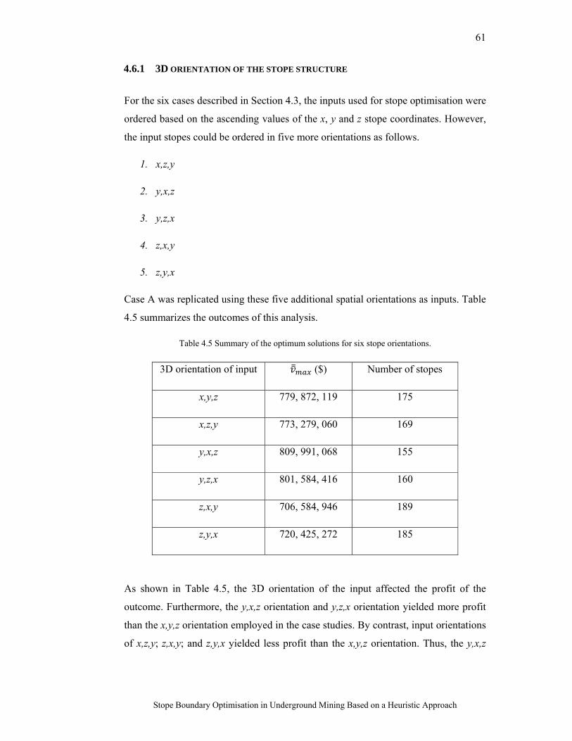
61
Stope Boundary Optimisation in Underground Mining Based on a Heuristic Approach
4.6.1 3D ORIENTATION OF THE STOPE STRUCTURE
For the six cases described in Section 4.3, the inputs used for stope optimisation were
ordered based on the ascending values of the x, y and z stope coordinates. However,
the input stopes could be ordered in five more orientations as follows.
1. x,z,y
2. y,x,z
3. y,z,x
4. z,x,y
5. z,y,x
Case A was replicated using these five additional spatial orientations as inputs. Table
4.5 summarizes the outcomes of this analysis.
Table 4.5 Summary of the optimum solutions for six stope orientations.
3D orientation of input ($) Number of stopes
x,y,z 779, 872, 119 175
x,z,y 773, 279, 060 169
y,x,z 809, 991, 068 155
y,z,x 801, 584, 416 160
z,x,y 706, 584, 946 189
z,y,x 720, 425, 272 185
As shown in Table 4.5, the 3D orientation of the input affected the profit of the
outcome. Furthermore, the y,x,z orientation and y,z,x orientation yielded more profit
than the x,y,z orientation employed in the case studies. By contrast, input orientations
of x,z,y; z,x,y; and z,y,x yielded less profit than the x,y,z orientation. Thus, the y,x,z
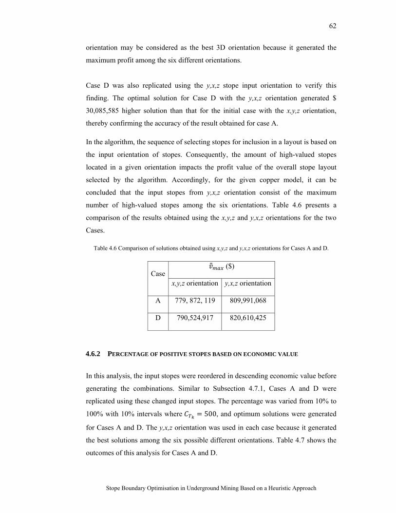
62
Stope Boundary Optimisation in Underground Mining Based on a Heuristic Approach
orientation may be considered as the best 3D orientation because it generated the
maximum profit among the six different orientations.
Case D was also replicated using the y,x,z stope input orientation to verify this
finding. The optimal solution for Case D with the y,x,z orientation generated $
30,085,585 higher solution than that for the initial case with the x,y,z orientation,
thereby confirming the accuracy of the result obtained for case A.
In the algorithm, the sequence of selecting stopes for inclusion in a layout is based on
the input orientation of stopes. Consequently, the amount of high-valued stopes
located in a given orientation impacts the profit value of the overall stope layout
selected by the algorithm. Accordingly, for the given copper model, it can be
concluded that the input stopes from y,x,z orientation consist of the maximum
number of high-valued stopes among the six orientations. Table 4.6 presents a
comparison of the results obtained using the x,y,z and y,x,z orientations for the two
Cases.
Table 4.6 Comparison of solutions obtained using x,y,z and y,x,z orientations for Cases A and D.
Case ($)
x,y,z orientation y,x,z orientation
A 779, 872, 119 809,991,068
D 790,524,917 820,610,425
4.6.2 PERCENTAGE OF POSITIVE STOPES BASED ON ECONOMIC VALUE
In this analysis, the input stopes were reordered in descending economic value before
generating the combinations. Similar to Subsection 4.7.1, Cases A and D were
replicated using these changed input stopes. The percentage was varied from 10% to
100% with 10% intervals where 500, and optimum solutions were generated
for Cases A and D. The y,x,z orientation was used in each case because it generated
the best solutions among the six possible different orientations. Table 4.7 shows the
outcomes of this analysis for Cases A and D.
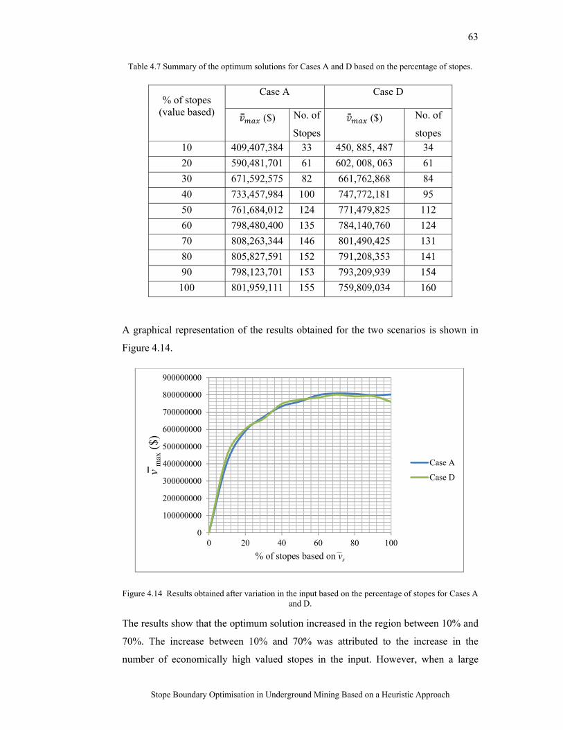
63
Stope Boundary Optimisation in Underground Mining Based on a Heuristic Approach
Table 4.7 Summary of the optimum solutions for Cases A and D based on the percentage of stopes.
% of stopes (value based)
Case A Case D
($) No. of
Stopes
($) No. of
stopes
10 409,407,384 33 450, 885, 487 34
20 590,481,701 61 602, 008, 063 61
30 671,592,575 82 661,762,868 84
40 733,457,984 100 747,772,181 95
50 761,684,012 124 771,479,825 112
60 798,480,400 135 784,140,760 124
70 808,263,344 146 801,490,425 131
80 805,827,591 152 791,208,353 141
90 798,123,701 153 793,209,939 154
100 801,959,111 155 759,809,034 160
A graphical representation of the results obtained for the two scenarios is shown in
Figure 4.14.
Figure 4.14 Results obtained after variation in the input based on the percentage of stopes for Cases A and D.
The results show that the optimum solution increased in the region between 10% and
70%. The increase between 10% and 70% was attributed to the increase in the
number of economically high valued stopes in the input. However, when a large
0
100000000
200000000
300000000
400000000
500000000
600000000
700000000
800000000
900000000
0 20 40 60 80 100
v m
ax($
)
% of stopes based on vs
Case A
Case D
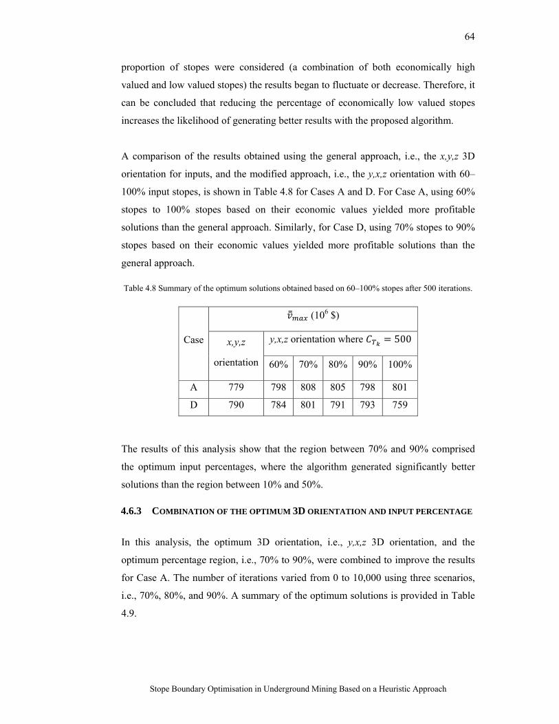
64
Stope Boundary Optimisation in Underground Mining Based on a Heuristic Approach
proportion of stopes were considered (a combination of both economically high
valued and low valued stopes) the results began to fluctuate or decrease. Therefore, it
can be concluded that reducing the percentage of economically low valued stopes
increases the likelihood of generating better results with the proposed algorithm.
A comparison of the results obtained using the general approach, i.e., the x,y,z 3D
orientation for inputs, and the modified approach, i.e., the y,x,z orientation with 60–
100% input stopes, is shown in Table 4.8 for Cases A and D. For Case A, using 60%
stopes to 100% stopes based on their economic values yielded more profitable
solutions than the general approach. Similarly, for Case D, using 70% stopes to 90%
stopes based on their economic values yielded more profitable solutions than the
general approach.
Table 4.8 Summary of the optimum solutions obtained based on 60–100% stopes after 500 iterations.
Case
(106 $)
x,y,z
orientation
y,x,z orientation where 500
60% 70% 80% 90% 100%
A 779 798 808 805 798 801
D 790 784 801 791 793 759
The results of this analysis show that the region between 70% and 90% comprised
the optimum input percentages, where the algorithm generated significantly better
solutions than the region between 10% and 50%.
4.6.3 COMBINATION OF THE OPTIMUM 3D ORIENTATION AND INPUT PERCENTAGE
In this analysis, the optimum 3D orientation, i.e., y,x,z 3D orientation, and the
optimum percentage region, i.e., 70% to 90%, were combined to improve the results
for Case A. The number of iterations varied from 0 to 10,000 using three scenarios,
i.e., 70%, 80%, and 90%. A summary of the optimum solutions is provided in Table
4.9.
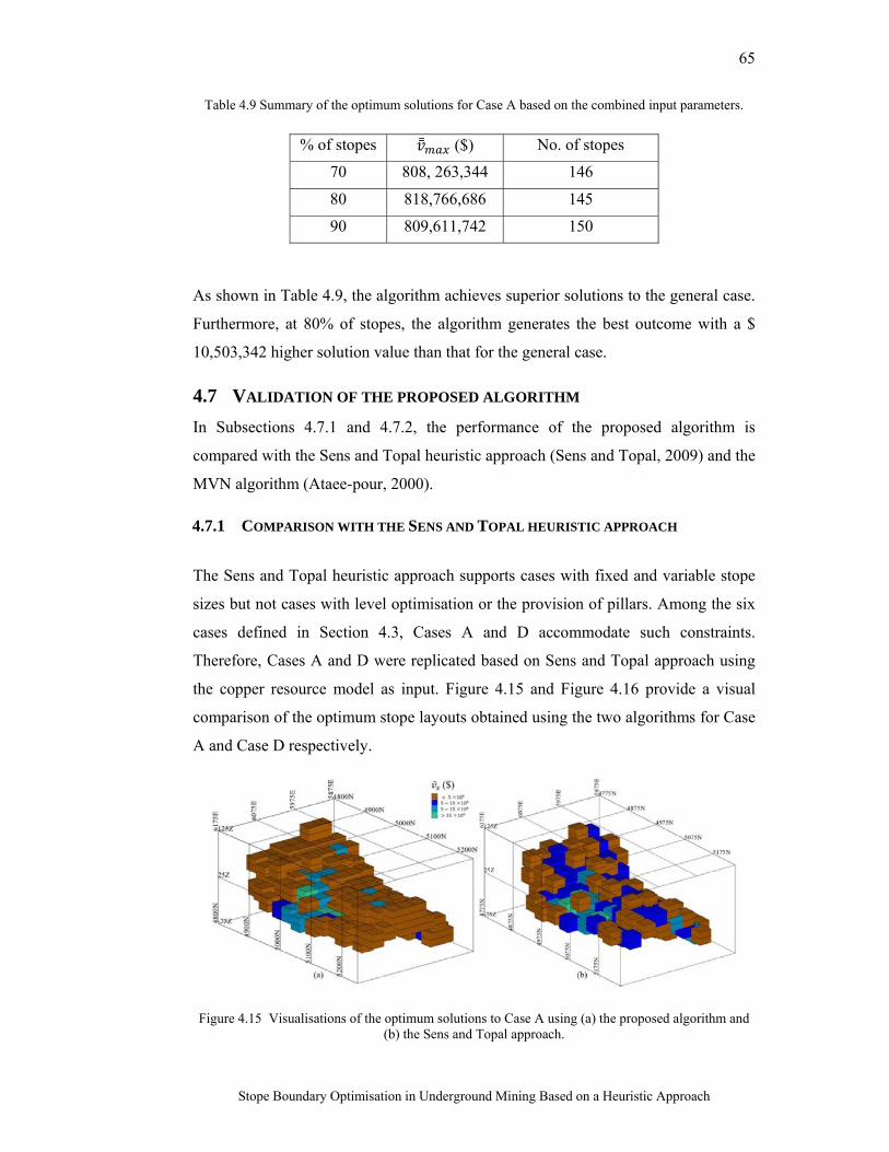
65
Stope Boundary Optimisation in Underground Mining Based on a Heuristic Approach
Table 4.9 Summary of the optimum solutions for Case A based on the combined input parameters.
% of stopes ($) No. of stopes
70 808, 263,344 146
80 818,766,686 145
90 809,611,742 150
As shown in Table 4.9, the algorithm achieves superior solutions to the general case.
Furthermore, at 80% of stopes, the algorithm generates the best outcome with a $
10,503,342 higher solution value than that for the general case.
4.7 VALIDATION OF THE PROPOSED ALGORITHM
In Subsections 4.7.1 and 4.7.2, the performance of the proposed algorithm is
compared with the Sens and Topal heuristic approach (Sens and Topal, 2009) and the
MVN algorithm (Ataee-pour, 2000).
4.7.1 COMPARISON WITH THE SENS AND TOPAL HEURISTIC APPROACH
The Sens and Topal heuristic approach supports cases with fixed and variable stope
sizes but not cases with level optimisation or the provision of pillars. Among the six
cases defined in Section 4.3, Cases A and D accommodate such constraints.
Therefore, Cases A and D were replicated based on Sens and Topal approach using
the copper resource model as input. Figure 4.15 and Figure 4.16 provide a visual
comparison of the optimum stope layouts obtained using the two algorithms for Case
A and Case D respectively.
Figure 4.15 Visualisations of the optimum solutions to Case A using (a) the proposed algorithm and (b) the Sens and Topal approach.
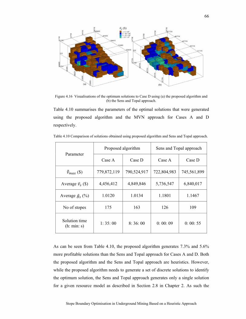
66
Stope Boundary Optimisation in Underground Mining Based on a Heuristic Approach
Figure 4.16 Visualisations of the optimum solutions to Case D using (a) the proposed algorithm and (b) the Sens and Topal approach.
Table 4.10 summarises the parameters of the optimal solutions that were generated
using the proposed algorithm and the MVN approach for Cases A and D
respectively.
Table 4.10 Comparison of solutions obtained using proposed algorithm and Sens and Topal approach.
Parameter Proposed algorithm Sens and Topal approach
Case A Case D Case A Case D
($) 779,872,119 790,524,917 722,804,983 745,561,899
Average ($) 4,456,412 4,849,846 5,736,547 6,840,017
Average (%) 1.0120 1.0134 1.1801 1.1467
No of stopes 175 163 126 109
Solution time (h: min: s)
1: 35: 00 8: 36: 00 0: 00: 09 0: 00: 55
As can be seen from Table 4.10, the proposed algorithm generates 7.3% and 5.6%
more profitable solutions than the Sens and Topal approach for Cases A and D. Both
the proposed algorithm and the Sens and Topal approach are heuristics. However,
while the proposed algorithm needs to generate a set of discrete solutions to identify
the optimum solution, the Sens and Topal approach generates only a single solution
for a given resource model as described in Section 2.8 in Chapter 2. As such the
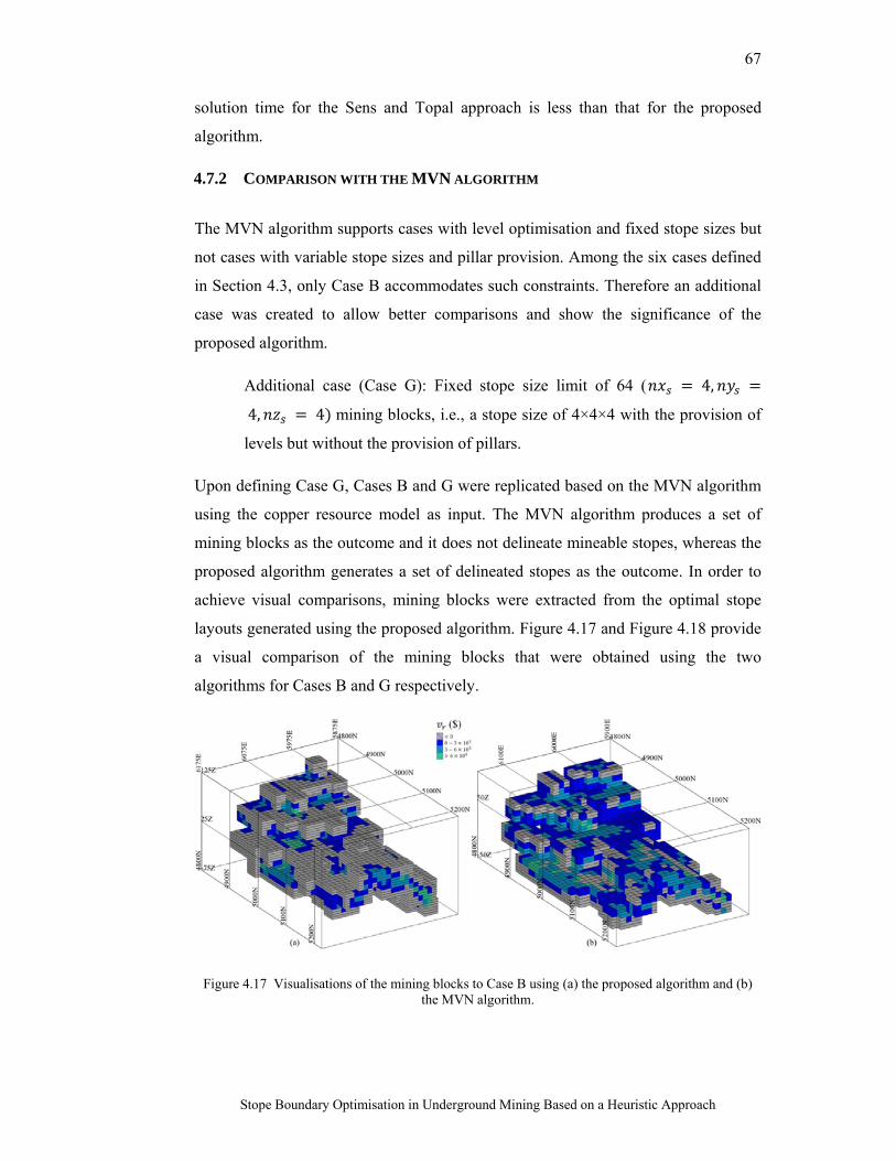
67
Stope Boundary Optimisation in Underground Mining Based on a Heuristic Approach
solution time for the Sens and Topal approach is less than that for the proposed
algorithm.
4.7.2 COMPARISON WITH THE MVN ALGORITHM
The MVN algorithm supports cases with level optimisation and fixed stope sizes but
not cases with variable stope sizes and pillar provision. Among the six cases defined
in Section 4.3, only Case B accommodates such constraints. Therefore an additional
case was created to allow better comparisons and show the significance of the
proposed algorithm.
Additional case (Case G): Fixed stope size limit of 64 ( 4,
4, 4 mining blocks, i.e., a stope size of 4×4×4 with the provision of
levels but without the provision of pillars.
Upon defining Case G, Cases B and G were replicated based on the MVN algorithm
using the copper resource model as input. The MVN algorithm produces a set of
mining blocks as the outcome and it does not delineate mineable stopes, whereas the
proposed algorithm generates a set of delineated stopes as the outcome. In order to
achieve visual comparisons, mining blocks were extracted from the optimal stope
layouts generated using the proposed algorithm. Figure 4.17 and Figure 4.18 provide
a visual comparison of the mining blocks that were obtained using the two
algorithms for Cases B and G respectively.
Figure 4.17 Visualisations of the mining blocks to Case B using (a) the proposed algorithm and (b) the MVN algorithm.
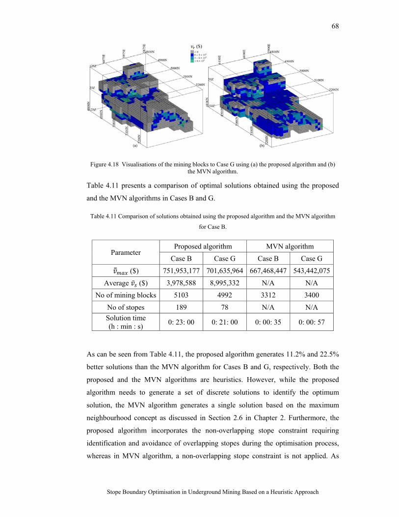
68
Stope Boundary Optimisation in Underground Mining Based on a Heuristic Approach
Figure 4.18 Visualisations of the mining blocks to Case G using (a) the proposed algorithm and (b) the MVN algorithm.
Table 4.11 presents a comparison of optimal solutions obtained using the proposed
and the MVN algorithms in Cases B and G.
Table 4.11 Comparison of solutions obtained using the proposed algorithm and the MVN algorithm
for Case B.
Parameter Proposed algorithm MVN algorithm
Case B Case G Case B Case G
($) 751,953,177 701,635,964 667,468,447 543,442,075
Average ($) 3,978,588 8,995,332 N/A N/A
No of mining blocks 5103 4992 3312 3400
No of stopes 189 78 N/A N/A
Solution time (h : min : s)
0: 23: 00 0: 21: 00 0: 00: 35 0: 00: 57
As can be seen from Table 4.11, the proposed algorithm generates 11.2% and 22.5%
better solutions than the MVN algorithm for Cases B and G, respectively. Both the
proposed and the MVN algorithms are heuristics. However, while the proposed
algorithm needs to generate a set of discrete solutions to identify the optimum
solution, the MVN algorithm generates a single solution based on the maximum
neighbourhood concept as discussed in Section 2.6 in Chapter 2. Furthermore, the
proposed algorithm incorporates the non-overlapping stope constraint requiring
identification and avoidance of overlapping stopes during the optimisation process,
whereas in MVN algorithm, a non-overlapping stope constraint is not applied. As
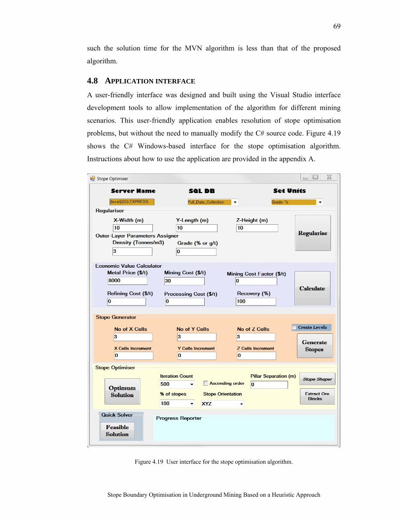
69
Stope Boundary Optimisation in Underground Mining Based on a Heuristic Approach
such the solution time for the MVN algorithm is less than that of the proposed
algorithm.
4.8 APPLICATION INTERFACE
A user-friendly interface was designed and built using the Visual Studio interface
development tools to allow implementation of the algorithm for different mining
scenarios. This user-friendly application enables resolution of stope optimisation
problems, but without the need to manually modify the C# source code. Figure 4.19
shows the C# Windows-based interface for the stope optimisation algorithm.
Instructions about how to use the application are provided in the appendix A.
Figure 4.19 User interface for the stope optimisation algorithm.
70
Stope Boundary Optimisation in Underground Mining Based on a Heuristic Approach
CHAPTER 5 CONCLUSIONS AND
RECOMMENDATIONS
This chapter is divided into Subsections 5.1 and 5.2. Subsection 5.1 summarises the
contributions of the thesis to the field of underground mining and outcomes of a case
study that demonstrates the applicability of the proposed algorithm to a real case
resource model representing a copper deposit. Subsection 5.2 provides
recommendations for improving the proposed algorithm based on observations of its
performance and applicability.
5.1 THESIS SUMMARY
This thesis presents four major contributions as follows.
1. The original contribution is the development of a robust heuristic algorithm
in order to generate an optimal stope layout for a given resource model. The
algorithm incorporates pillar separation, level separation and stope size
variation, successfully to generate solutions subject to physical mining
constraints. Previous heuristic approaches lack the incorporation of physical
mining constraints. Therefore, the proposed algorithm becomes an
innovative mine planning tool for generating optimum stope layouts that
represent realistic mining scenarios.
2. The proposed algorithm establishes the exponential relationship between the
solution time and possible solutions to the problem. The thesis presents an
innovative method to handle the computational complexity and implements
the method successfully to a resource model which represents a copper
deposit. Further, the performance of the algorithm is improved using the task
parallelism concept from object oriented programming, thereby presenting
an efficient method to develop solutions to block models consisting of
thousands of mining blocks.
3. The algorithm incorporates an innovative method for identifying overlapping
stopes and avoiding their inclusion in the optimum stope layout, thus
eliminating the problem within the industrially recognised floating stope
algorithm.
71
Stope Boundary Optimisation in Underground Mining Based on a Heuristic Approach
4. Development of user-friendly software that implements the stope
optimisation algorithm for different mining scenarios including Microsoft C#
object-oriented programming language and the Microsoft SQL server. The
advantage of using this combination is that it enables the execution of the
software on windows-based computers with different architectures. As a
result of this development, manual changes to the source code are not
required to implement the algorithm in different mining scenarios.
Due to the combinatorial optimisation nature of the problem the algorithm employs a
heuristic approach. The design of the heuristic algorithm has a compound nature, i.e.,
constructive and improvement characteristics which are incorporated to ensure that
better quality solutions are achieved in the shortest possible time.
The algorithm was implemented on a resource model that represented a copper
deposit, where six cases (Cases A to F) were defined based on a variety of mining
scenarios to demonstrate the suitability of the algorithm for different mining
situations. For the given resource model, Case D with a variable stope size of
3 3 3 3 3 4 yielded the most profitable solution among the six cases. The
provision of pillars and levels reduced the solution value compared with cases
without the provision of pillars and levels. This was because the provision of pillars
and levels prior to optimisation reduced the number of positive-valued stopes in the
input, and thus the number of possible solutions.
In a further analysis that aimed to improve the solution values for Cases A and D, the
structure of the input positive-valued stopes, were modified to identify the optimum
spatial orientation and the optimum input percentage for the high-valued stopes.
Based on the outcomes, the y,x,z orientation was selected as the optimal spatial
orientation because changing the orientation from x,y,z to y,x,z increased the solution
value by 3.8% in both cases. For the input stopes, a range of 70–90% was identified
as the optimal percentage range. A modified input structure that comprised the y,x,z
stope orientation and 80% of the high-valued stopes improved the solution value in
Case A by 1.2%. This analysis proves that altering the orientation or the amount of
high-valued stopes in the input impacts the sequence in which the stopes are selected
to generate a solution, thereby increasing the solution value. Therefore, it can be
72
Stope Boundary Optimisation in Underground Mining Based on a Heuristic Approach
concluded that restructuring the input has potential to obtain better solutions when
applying the proposed algorithm to resource models.
The algorithm was validated based on comparisons with two existing heuristic
algorithms: the MVN algorithm and Sens and Topal’s heuristic approach. The
proposed algorithm obtained superior solutions than both of the existing algorithms
for selected cases. The MVN algorithm was implemented only for Cases B and G
because it does not support variable stope sizes and the provision of pillars. The
proposed algorithm generated solutions which were 11.2% and 22.5% more
profitable than the solution obtained using the MVN algorithm. The Sens and Topal
heuristic approach was implemented for Cases A and D specifically because it does
not support the provision of levels and pillars. The proposed algorithm generated
solutions, which were 7.3% and 5.6% more profitable than the solutions obtained
using the Sens and Topal heuristic approach for Cases A and D, respectively. An
advantage of the proposed algorithm compared with the MVN algorithm is that it
allows the provision of pillars or variable stopes sizes when developing solutions.
Similarly, an advantage of the proposed algorithm compared with the Sens and Topal
heuristic approach is that it can incorporate level definitions and the provision of
pillars when developing solutions. This reflects the flexibility of the proposed
algorithm for generating solutions to realistic underground mining scenarios.
5.2 RECOMMENDATIONS
This research has made a significant contribution to the development of an algorithm
to optimise stope boundary layout in underground mining as discussed in this thesis.
However, the proposed algorithm can be further improved to optimise its
performance and applicability in the following areas.
Even though the scope of this research was limited to stope boundary optimisation,
production scheduling must be incorporated to the stope optimisation process
because they share a close relationship with one area influencing the other.
Currently, it is a common mine planning practice to consider optimisation of each
area separately. Consequently, the resulting revenues may be, less than a
simultaneous consideration of both areas in the optimisation process. In order to
handle the specific geotechnical aspects, i.e. size and orientation of the ore body,
load carrying capacity of rock mass, etc., given ore body models can be divided in to
73
Stope Boundary Optimisation in Underground Mining Based on a Heuristic Approach
sub sections allowing the optimisation of stope layout for those sections separately.
As such, further modifications to the proposed algorithm are required to satisfy the
geotechnical parameters which influence the stope layout as well as production
scheduling.
A versatile extension to the developed interface would be a stand-alone visualiser,
which would facilitate the rapid visualisation of 3D stope layouts. The current
version of the stope optimisation software relies on visualisation using external mine
design software tools. This process requires time to transfer and convert the output
files into compatible formats for current visualisation tools.
The application of the multi-threading concept improved the performance of the
algorithm, but this needs to be investigated further and tested rigorously. In the
present study, only two sets of non-overlapping stopes were defined as the input for
multi-threading. Further divisions of the input file may result in greater performance
improvements and shorter solution times. However, the addition of more sets to the
computational process may result in proportional increases in the processing power
and memory requirements.
The algorithm generates solutions for resource models that contain one mineral type,
thus further improvements are required to the structure of the algorithm for multi-
commodity resource models. An option to select either single-commodity or multi-
commodity can be added to the developed interface to facilitate this requirement.
74
Stope Boundary Optimisation in Underground Mining Based on a Heuristic Approach
REFERENCES
Albahari, J., & Albahari, B. (2010). C# 4.0 in a nutshell.4th edition ed., U.S.A.: (O’REILLY).
Alford, C. (1995, 9-14 July). Optimisation in underground mine design, Brisbane. http://dx.doi.org:10.1016/0148-9062(96)80055-6
Alford, C., Brazil, M., & Lee, D. (2007). Optimisation in Underground Mining. In A. Weintraub, C. Romero, T. Bjørndal, R. Epstein & J. Miranda (Eds.), Handbook Of Operations Research In Natural Resources (Vol. 99, pp. 561-577): Springer US. http://dx.doi.org/:10.1007/978-0-387-71815-6_30
Alford, C., & Hall, B. (2009, 21-22 April 2009). Stope Optimisation Tools for Selection of Optimum Cut-Off grade in Underground Mine Design. Paper presented at the Project Evaluation Conference, Melbourne, Vic21-22 April 2009 Accessed
Asad, M. W. A. (2011). A heuristic approach to long-range production planning of cement quarry operations. Prod. Plan. Control, 22(4), 353-364. http://dx.doi.org/10.1080/09537287.2010.484819
Asad, M. W. A., Dimitrakopoulos, R., & Eldert, J. v. (2013). Stochastic production phase design for an open pit mining complex with multiple processing streams. Engineering Optimization, 46(8), 1139-1152. http://dx.doi.org/10.1080/0305215X.2013.819094
Ataee-pour, M. (2000). A heuristic algorithm to optimise stope boundaries. Doctor of Philosophy University of Wollongong, New South Wales, Australia.
Ataee-pour, M. (2004). Optimisation of stope limits using a heuristic approach. Transactions of the Institution of Mining and Metallurgy Section a-Mining Technology, 113(2), A123-A128. http://dx.doi.org/ 10.1179/037178404225004959
Ataee-pour, M. (2005). A critical survey of the existing stope layout optimization techniques. Journal of Mining Science, 41(5), 447-466. http://dx.doi.org/ 10.1007/s10913-006-0008-9
Bai, X. Y., Marcotte, D., & Simon, R. (2013). Underground stope optimization with network flow method. Computers & Geosciences, 52, 361-371. http://dx.doi.org/DOI 10.1016/j.cageo.2012.10.019
Basel, J., III, & Willemain, T. (2001). Random Tours in the Traveling Salesman Problem: Analysis and Application. Computational Optimization and Applications, 20(2), 211-217. http://dx.doi.org/10.1023/A:1011263204536
75
Stope Boundary Optimisation in Underground Mining Based on a Heuristic Approach
Bernstein, D., Jeffery, S., Lange, T., & Meurer, A. (2013). Quantum Algorithms for the Subset-Sum Problem. In P. Gaborit (Ed.), Post-Quantum Cryptography (Vol. 7932, pp. 16-33): Springer Berlin Heidelberg.
C# Threads. (2013). Retrieved January 21, 2013 http://www.dotnetperls.com/thread
CAE Studio 3. (2014). software available at http://www.cae.com/mining/
Cawrse, I. (2001). Multiple Pass Floating Stope Process. Paper presented at the 4th Biennial Strategic Mine Planning Conference, Melbourne
Cawrse, I. (2007). Multiple pass floating stope process, held in Strategic Mine Planning Conference, (pp. 87-94). Perth, Australia
Cheimanoff, N. M., Deliac, E. P., & Mallet, J. L. (1989). GEOCAD: an alternative CAD and artificial intelligence tool that helps moving from geological resources to mineable reserves. Paper presented at the 21st International APCOM Symposium, USA
Darling, P. (2011). SME mining engineering handbook (Vol. 2): SME.
Deitel, P. J., & Deitel, H. M. (2008). Visual C#® 2008 How to Program. U.S.A.: Prentice Hall Press.
Derigs, U., & Vogel, U. (2014). Experience with a framework for developing heuristics for solving rich vehicle routing problems. Journal of Heuristics, 20(1), 75-106. http://dx.doi.org/10.1007/s10732-013-9232-z
Dimitrakopoulos, R., & Grieco, N. (2009). Stope design and geologi-cal uncertainty: quantification of risk in conventional de-signs and probabilistic alternative. Journal of Mining Science, 45(2), 152-163.
EQATEC .NET version 1.1. (2014). Software available at http://eqatec-profiler.eqatec-as.blueprograms.com/
GEOVIA Surpac™ version 6.3.1. (2012). Software available at http://www.gemcomsoftware.com/products/surpac
Gertch, R. E., & Bullock, R. L. (1998). Techniques in Techniques in Underground Mining. USA: Society for Mining, Metallurgy, and Exploration, Inc.
Gonçalves, J., & Resende, M. C. (2011). Biased random-key genetic algorithms for combinatorial optimization. Journal of Heuristics, 17(5), 487-525. http://dx.doi.org/10.1007/s10732-010-9143-1
Grieco, N., & Dimitrakopoulos, R. (2007). Managing grade risk in stope design optimisation: probabilistic mathematical programming model and application in sublevel stoping. Mining Technology, 116(2), 49-57.
Hejlsberg, A., Torgersen, M., Wiltamuth, S., & Golde, P. (2010). The C# programming language. U.S.A.: Addison-Wesley.
76
Stope Boundary Optimisation in Underground Mining Based on a Heuristic Approach
Hustrulid, W. A. (2006). Open pit mine planning & design / William Hustrulid, Mark Kuchta. London: London : Taylor and Francis.
Hustrulid, W. A., & Bullock, R. L. (2001). Underground Mining Methods. Colorado, USA: Society for Mining, Metallurgy, and Exploration Inc.
James, M. H. (2013). C#/.NET Little Wonders. Retrieved January 23, 2013 http://geekswithblogs.net/BlackRabbitCoder/archive/2012/12/20/c.net-little-wonders-the-parallel.invoke-method.aspx
Karapetyan, D. (2010). Design, Evaluation and Analysis of Combinatorial Optimization Heuristic Algorithms. Doctor of Philosophy University of London, United Kingdom.
Krishna, R., & Chanda, M. W. (1997). Re-thinking in the optimization of stope dimensions. Eighth International Congress on Rock Mechanics, Vol 3, Proceedings, 1381-1384. <Go to ISI>://A1997BH39W00069
Kumral, M. (2004). Genetic algorithms for optimization of a mine system under uncertainty. Production Planning & Control, 15(1), 34-41. http://dx.doi.org/10.1080/09537280310001654844
Kumral, M. (2010). Robust stochastic mine production scheduling. Eng. Optimiz., 42(6), 567-579. http://dx.doi.org/10.1080/03052150903353336
Kumral, M. (2013). Optimizing ore–waste discrimination and block sequencing through simulated annealing. Applied Soft Computing, 13(8), 3737-3744. http://dx.doi.org/http://dx.doi.org/10.1016/j.asoc.2013.03.005
Lam, F., & Newman, A. (2008). Traveling salesman path problems. Mathematical Programming, 113(1), 39-59. http://dx.doi.org/10.1007/s10107-006-0046-8
Little, J. (2012). Simultaneous optimisation of stope layouts and production schedules for long-term underground mine planning. Doctor of Philosophy University of Queensland, Queensland, Australia.
Little, J., Knights, P., & Topal, E. (2013). Integrated optimization of underground mine design and scheduling. Journal of the Southern African Institute of Mining and Metallurgy, 113(10), 775-785.
Little, J., & Topal, E. (2011). Strategies to assist in obtaining an optimal solution for an underground mine planning problem using Mixed Integer Programming.
Little, J., Topal, E., & Knights, P. (2011). Simultaneous optimisation of stope layouts and long term production schedules. Mining Technology, 120(3), 129-136. http://dx.doi.org/doi:10.1179/1743286311Y.0000000011
Martí, R., Gallego, M., Duarte, A., & Pardo, E. (2013). Heuristics and metaheuristics for the maximum diversity problem. Journal of Heuristics, 19(4), 591-615. http://dx.doi.org/10.1007/s10732-011-9172-4
77
Stope Boundary Optimisation in Underground Mining Based on a Heuristic Approach
Morelan, R. A., Ekberg, T., Brown, J., & Berger, I. (2009). SQL Queries Joes 2 Pros: SQL Query Techniques For Microsoft SQL Server 2008, Volume 2: BookSurge Publishing.
Okubo, S., & Yamatomi, J. (n.d.). Underground Mining Methods and Equipment. Civil Engineering, 2 Retrieved from http://www.eolss.net/sample-chapters/c05/e6-37-06-02.pdf
Ovanic, J., & Young, D. S. (1995). Economic optimization of stope geometry using separable programming with special branch and bound techniques. Paper presented at the 3rd Canadian Conference on Computer Applications in the Mineral Industry, McGill University, Montreal
Ovanic, J., & Young, D. S. (1999). Economic optimisation of open stope geometry. Paper presented at the 28th International APCOM Symposium, Colorado School of Mines, Golden
Parallel Class. (2013). Retrieved January 23, 2013 http://msdn.microsoft.com/en-us/library/vstudio/system.threading.tasks.parallel(v=vs.110).aspx
Punnen, A. (2007). The Traveling Salesman Problem: Applications, Formulations and Variations. In G. Gutin & A. Punnen (Eds.), The Traveling Salesman Problem and Its Variations (Vol. 12, pp. 1-28): Springer US. http://dx.doi.org/:10.1007/0-306-48213-4_1
Rardin, R., & Uzsoy, R. (2001). Experimental Evaluation of Heuristic Optimization Algorithms: A Tutorial. Journal of Heuristics, 7(3), 261-304. http://dx.doi.org/10.1023/A:1011319115230
Richmond, A. J., & Beasley, J. E. (2004). An Iterative Construction Heuristic for the Ore Selection Problem. Journal of Heuristics, 10(2), 153-167. http://dx.doi.org/10.1023/B:HEUR.0000026265.47626.23
Riddle, J. M. (1977). A dynamic programming solution of a block caving mine layout. Paper presented at the 14th APCOM Symposium, New York
Semančo, P., & Modrák, V. (2011). Hybrid GA-Based Improvement Heuristic with Makespan Criterion for Flow-Shop Scheduling Problems. In M. Cruz-Cunha, J. Varajão, P. Powell & R. Martinho (Eds.), ENTERprise Information Systems (Vol. 220, pp. 11-18): Springer Berlin Heidelberg. http://dx.doi.org/:10.1007/978-3-642-24355-4_2
Sens, J., & Topal, E. (2009). A New Algorithm for Stope Boundary Optimisation. Ausimm New Leaders Conference 2009, 2009(4), 25-28. <Go to ISI>://000271285400004
Topal, E. (2008). Early and late start algorithms to improve the solution time for long-term underground mine production scheduling. The Journal of the South African Institute of Mining and Metallurgy, 108(2), 101-107.
78
Stope Boundary Optimisation in Underground Mining Based on a Heuristic Approach
Žerovnik, G., & Žerovnik, J. (2011). Constructive heuristics for the canister filling problem. Central European Journal of Operations Research, 19(3), 371-389. http://dx.doi.org/10.1007/s10100-010-0164-5
Every reasonable effort has been made to acknowledge the owners of copyright
material. I would be pleased to hear from any copyright owner who has been omitted
or incorrectly acknowledged.
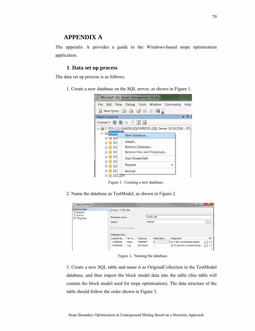
79
Stope Boundary Optimisation in Underground Mining Based on a Heuristic Approach
APPENDIX A
The appendix A provides a guide to the Windows-based stope optimisation
application.
1. Data set up process
The data set up process is as follows.
1. Create a new database on the SQL server, as shown in Figure 1.
Figure 1. Creating a new database.
2. Name the database as TestModel, as shown in Figure 2.
Figure 2. Naming the database.
3. Create a new SQL table and name it as OriginalCollection in the TestModel
database, and then import the block model data into the table (this table will
contain the block model used for stope optimisation). The data structure of the
table should follow the order shown in Figure 3.
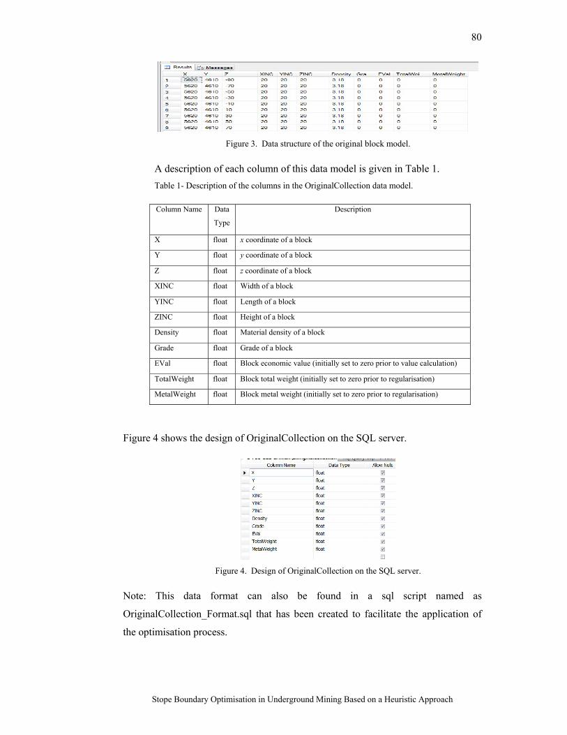
80
Stope Boundary Optimisation in Underground Mining Based on a Heuristic Approach
Figure 3. Data structure of the original block model.
A description of each column of this data model is given in Table 1.
Table 1- Description of the columns in the OriginalCollection data model.
Column Name Data
Type
Description
X float x coordinate of a block
Y float y coordinate of a block
Z float z coordinate of a block
XINC float Width of a block
YINC float Length of a block
ZINC float Height of a block
Density float Material density of a block
Grade float Grade of a block
EVal float Block economic value (initially set to zero prior to value calculation)
TotalWeight float Block total weight (initially set to zero prior to regularisation)
MetalWeight float Block metal weight (initially set to zero prior to regularisation)
Figure 4 shows the design of OriginalCollection on the SQL server.
Figure 4. Design of OriginalCollection on the SQL server.
Note: This data format can also be found in a sql script named as
OriginalCollection_Format.sql that has been created to facilitate the application of
the optimisation process.
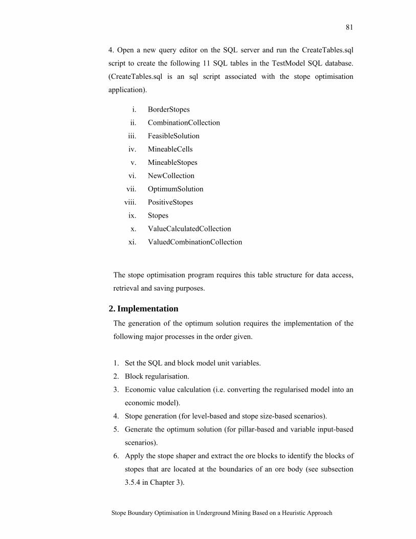
81
Stope Boundary Optimisation in Underground Mining Based on a Heuristic Approach
4. Open a new query editor on the SQL server and run the CreateTables.sql
script to create the following 11 SQL tables in the TestModel SQL database.
(CreateTables.sql is an sql script associated with the stope optimisation
application).
i. BorderStopes
ii. CombinationCollection
iii. FeasibleSolution
iv. MineableCells
v. MineableStopes
vi. NewCollection
vii. OptimumSolution
viii. PositiveStopes
ix. Stopes
x. ValueCalculatedCollection
xi. ValuedCombinationCollection
The stope optimisation program requires this table structure for data access,
retrieval and saving purposes.
2. Implementation
The generation of the optimum solution requires the implementation of the
following major processes in the order given.
1. Set the SQL and block model unit variables.
2. Block regularisation.
3. Economic value calculation (i.e. converting the regularised model into an
economic model).
4. Stope generation (for level-based and stope size-based scenarios).
5. Generate the optimum solution (for pillar-based and variable input-based
scenarios).
6. Apply the stope shaper and extract the ore blocks to identify the blocks of
stopes that are located at the boundaries of an ore body (see subsection
3.5.4 in Chapter 3).
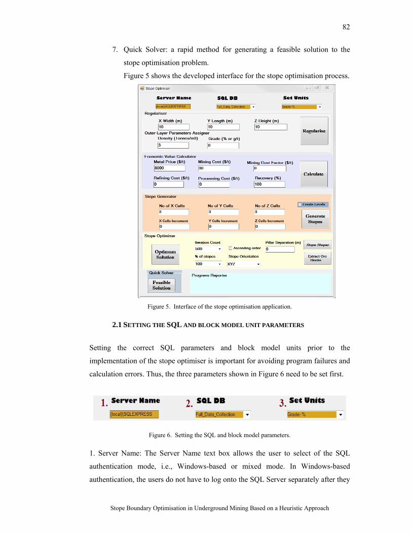
82
Stope Boundary Optimisation in Underground Mining Based on a Heuristic Approach
7. Quick Solver: a rapid method for generating a feasible solution to the
stope optimisation problem.
Figure 5 shows the developed interface for the stope optimisation process.
Figure 5. Interface of the stope optimisation application.
2.1 SETTING THE SQL AND BLOCK MODEL UNIT PARAMETERS
Setting the correct SQL parameters and block model units prior to the
implementation of the stope optimiser is important for avoiding program failures and
calculation errors. Thus, the three parameters shown in Figure 6 need to be set first.
Figure 6. Setting the SQL and block model parameters.
1. Server Name: The Server Name text box allows the user to select of the SQL
authentication mode, i.e., Windows-based or mixed mode. In Windows-based
authentication, the users do not have to log onto the SQL Server separately after they
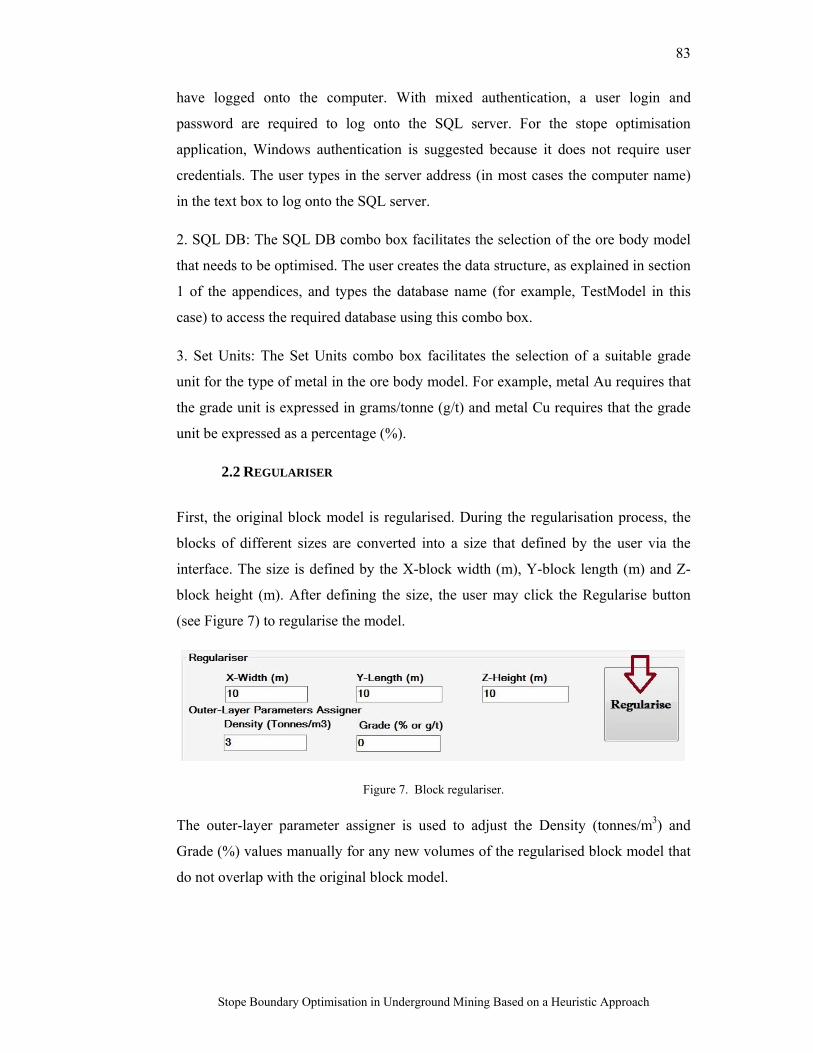
83
Stope Boundary Optimisation in Underground Mining Based on a Heuristic Approach
have logged onto the computer. With mixed authentication, a user login and
password are required to log onto the SQL server. For the stope optimisation
application, Windows authentication is suggested because it does not require user
credentials. The user types in the server address (in most cases the computer name)
in the text box to log onto the SQL server.
2. SQL DB: The SQL DB combo box facilitates the selection of the ore body model
that needs to be optimised. The user creates the data structure, as explained in section
1 of the appendices, and types the database name (for example, TestModel in this
case) to access the required database using this combo box.
3. Set Units: The Set Units combo box facilitates the selection of a suitable grade
unit for the type of metal in the ore body model. For example, metal Au requires that
the grade unit is expressed in grams/tonne (g/t) and metal Cu requires that the grade
unit be expressed as a percentage (%).
2.2 REGULARISER
First, the original block model is regularised. During the regularisation process, the
blocks of different sizes are converted into a size that defined by the user via the
interface. The size is defined by the X-block width (m), Y-block length (m) and Z-
block height (m). After defining the size, the user may click the Regularise button
(see Figure 7) to regularise the model.
Figure 7. Block regulariser.
The outer-layer parameter assigner is used to adjust the Density (tonnes/m3) and
Grade (%) values manually for any new volumes of the regularised block model that
do not overlap with the original block model.
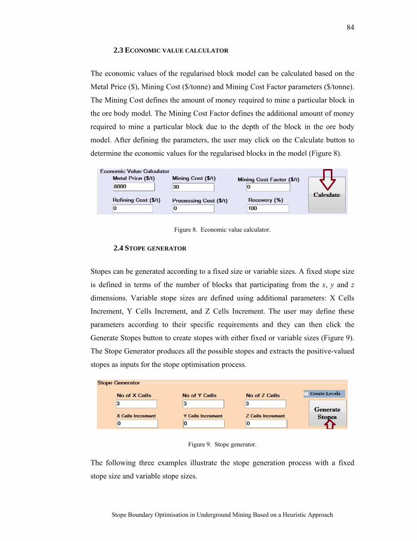
84
Stope Boundary Optimisation in Underground Mining Based on a Heuristic Approach
2.3 ECONOMIC VALUE CALCULATOR
The economic values of the regularised block model can be calculated based on the
Metal Price ($), Mining Cost ($/tonne) and Mining Cost Factor parameters ($/tonne).
The Mining Cost defines the amount of money required to mine a particular block in
the ore body model. The Mining Cost Factor defines the additional amount of money
required to mine a particular block due to the depth of the block in the ore body
model. After defining the parameters, the user may click on the Calculate button to
determine the economic values for the regularised blocks in the model (Figure 8).
Figure 8. Economic value calculator.
2.4 STOPE GENERATOR
Stopes can be generated according to a fixed size or variable sizes. A fixed stope size
is defined in terms of the number of blocks that participating from the x, y and z
dimensions. Variable stope sizes are defined using additional parameters: X Cells
Increment, Y Cells Increment, and Z Cells Increment. The user may define these
parameters according to their specific requirements and they can then click the
Generate Stopes button to create stopes with either fixed or variable sizes (Figure 9).
The Stope Generator produces all the possible stopes and extracts the positive-valued
stopes as inputs for the stope optimisation process.
Figure 9. Stope generator.
The following three examples illustrate the stope generation process with a fixed
stope size and variable stope sizes.
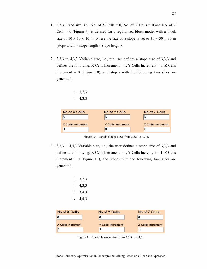
85
Stope Boundary Optimisation in Underground Mining Based on a Heuristic Approach
1. 3,3,3 Fixed size, i.e., No. of X Cells = 0, No. of Y Cells = 0 and No. of Z
Cells = 0 (Figure 9), is defined for a regularised block model with a block
size of 10 10 10 m, where the size of a stope is set to 30 30 30 m
(stope width stope length stope height).
2. 3,3,3 to 4,3,3 Variable size, i.e., the user defines a stope size of 3,3,3 and
defines the following: X Cells Increment = 1, Y Cells Increment = 0, Z Cells
Increment = 0 (Figure 10), and stopes with the following two sizes are
generated.
i. 3,3,3
ii. 4,3,3
Figure 10. Variable stope sizes from 3,3,3 to 4,3,3.
3. 3,3,3 – 4,4,3 Variable size, i.e., the user defines a stope size of 3,3,3 and
defines the following: X Cells Increment = 1, Y Cells Increment = 1, Z Cells
Increment = 0 (Figure 11), and stopes with the following four sizes are
generated.
i. 3,3,3
ii. 4,3,3
iii. 3,4,3
iv. 4,4,3
Figure 11. Variable stope sizes from 3,3,3 to 4,4,3.
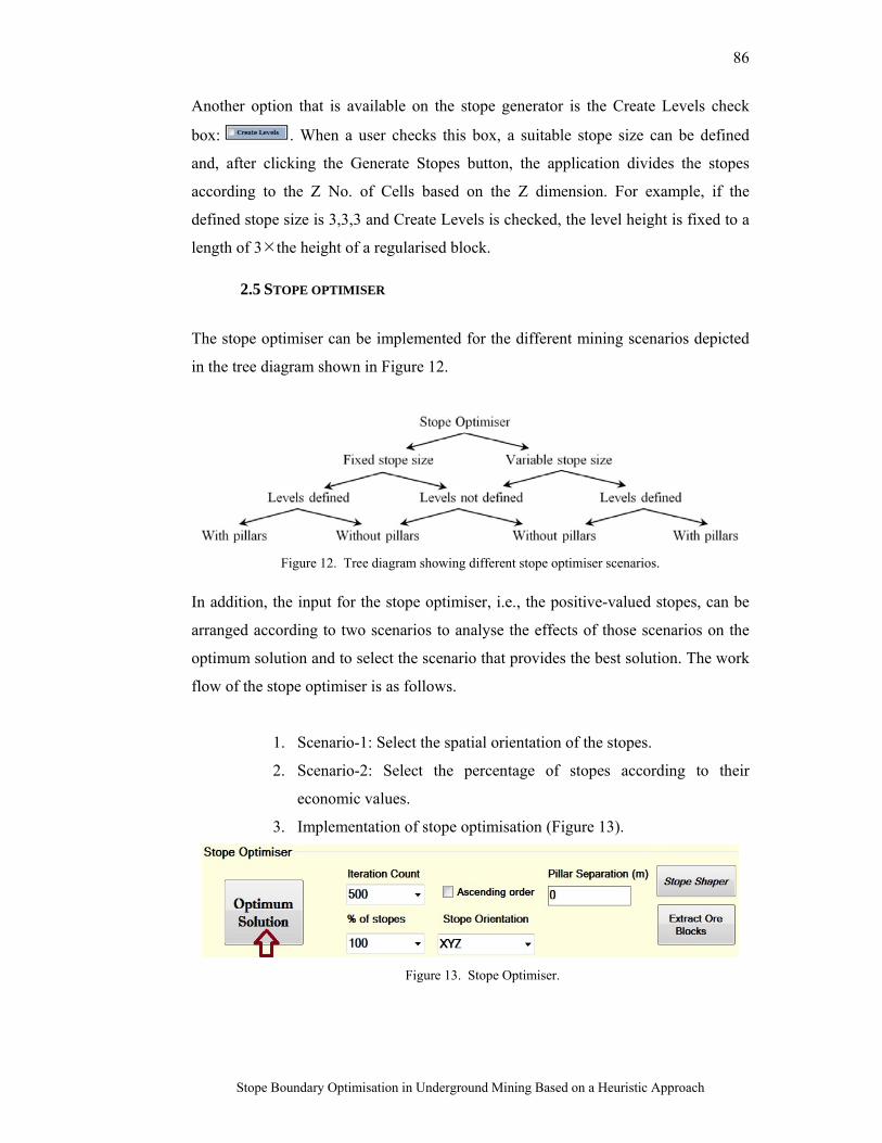
86
Stope Boundary Optimisation in Underground Mining Based on a Heuristic Approach
Another option that is available on the stope generator is the Create Levels check
box: . When a user checks this box, a suitable stope size can be defined
and, after clicking the Generate Stopes button, the application divides the stopes
according to the Z No. of Cells based on the Z dimension. For example, if the
defined stope size is 3,3,3 and Create Levels is checked, the level height is fixed to a
length of 3the height of a regularised block.
2.5 STOPE OPTIMISER
The stope optimiser can be implemented for the different mining scenarios depicted
in the tree diagram shown in Figure 12.
Figure 12. Tree diagram showing different stope optimiser scenarios.
In addition, the input for the stope optimiser, i.e., the positive-valued stopes, can be
arranged according to two scenarios to analyse the effects of those scenarios on the
optimum solution and to select the scenario that provides the best solution. The work
flow of the stope optimiser is as follows.
1. Scenario-1: Select the spatial orientation of the stopes.
2. Scenario-2: Select the percentage of stopes according to their
economic values.
3. Implementation of stope optimisation (Figure 13).
Figure 13. Stope Optimiser.
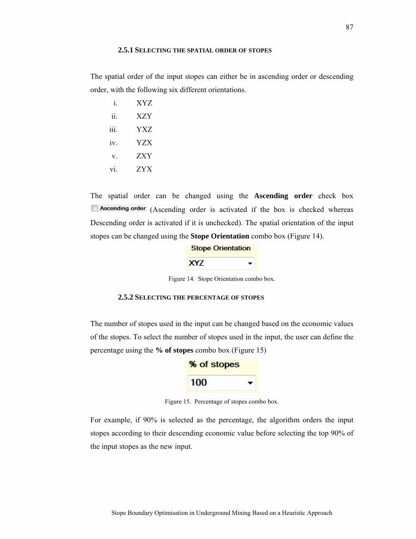
87
Stope Boundary Optimisation in Underground Mining Based on a Heuristic Approach
2.5.1 SELECTING THE SPATIAL ORDER OF STOPES
The spatial order of the input stopes can either be in ascending order or descending
order, with the following six different orientations.
i. XYZ
ii. XZY
iii. YXZ
iv. YZX
v. ZXY
vi. ZYX
The spatial order can be changed using the Ascending order check box
(Ascending order is activated if the box is checked whereas
Descending order is activated if it is unchecked). The spatial orientation of the input
stopes can be changed using the Stope Orientation combo box (Figure 14).
Figure 14. Stope Orientation combo box.
2.5.2 SELECTING THE PERCENTAGE OF STOPES
The number of stopes used in the input can be changed based on the economic values
of the stopes. To select the number of stopes used in the input, the user can define the
percentage using the % of stopes combo box (Figure 15)
Figure 15. Percentage of stopes combo box.
For example, if 90% is selected as the percentage, the algorithm orders the input
stopes according to their descending economic value before selecting the top 90% of
the input stopes as the new input.
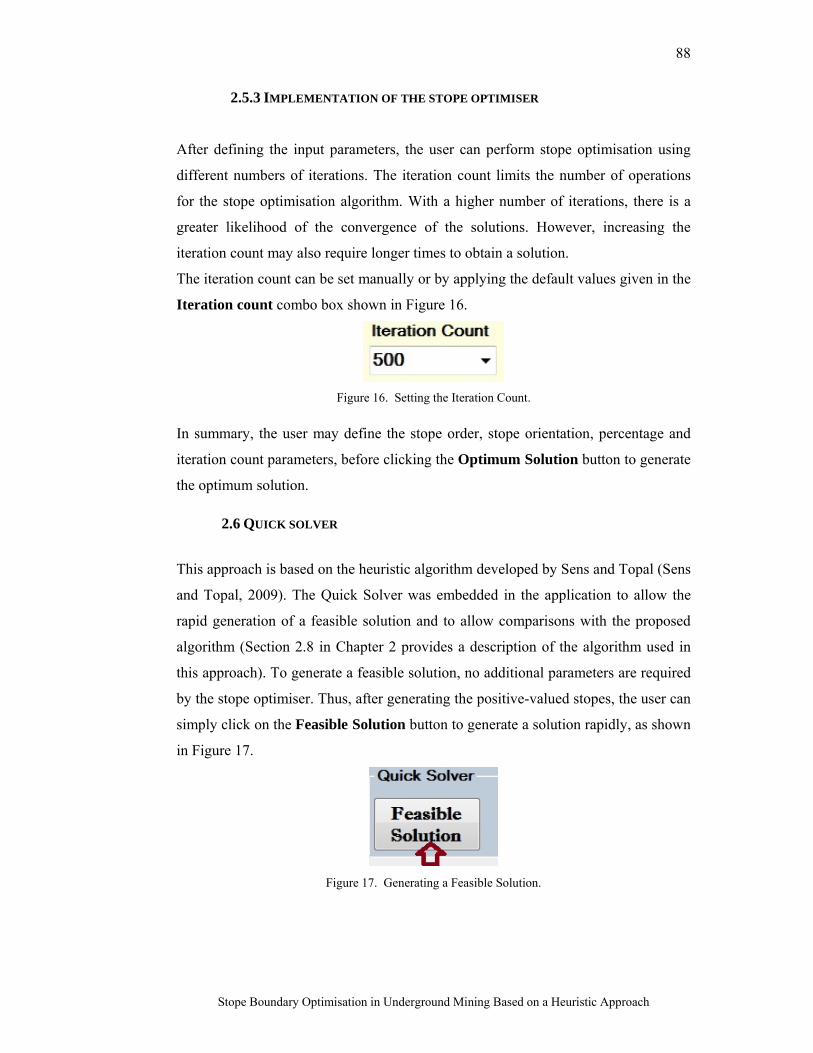
88
Stope Boundary Optimisation in Underground Mining Based on a Heuristic Approach
2.5.3 IMPLEMENTATION OF THE STOPE OPTIMISER
After defining the input parameters, the user can perform stope optimisation using
different numbers of iterations. The iteration count limits the number of operations
for the stope optimisation algorithm. With a higher number of iterations, there is a
greater likelihood of the convergence of the solutions. However, increasing the
iteration count may also require longer times to obtain a solution.
The iteration count can be set manually or by applying the default values given in the
Iteration count combo box shown in Figure 16.
Figure 16. Setting the Iteration Count.
In summary, the user may define the stope order, stope orientation, percentage and
iteration count parameters, before clicking the Optimum Solution button to generate
the optimum solution.
2.6 QUICK SOLVER
This approach is based on the heuristic algorithm developed by Sens and Topal (Sens
and Topal, 2009). The Quick Solver was embedded in the application to allow the
rapid generation of a feasible solution and to allow comparisons with the proposed
algorithm (Section 2.8 in Chapter 2 provides a description of the algorithm used in
this approach). To generate a feasible solution, no additional parameters are required
by the stope optimiser. Thus, after generating the positive-valued stopes, the user can
simply click on the Feasible Solution button to generate a solution rapidly, as shown
in Figure 17.
Figure 17. Generating a Feasible Solution.
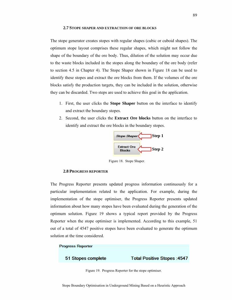
89
Stope Boundary Optimisation in Underground Mining Based on a Heuristic Approach
2.7 STOPE SHAPER AND EXTRACTION OF ORE BLOCKS
The stope generator creates stopes with regular shapes (cubic or cuboid shapes). The
optimum stope layout comprises these regular shapes, which might not follow the
shape of the boundary of the ore body. Thus, dilution of the solution may occur due
to the waste blocks included in the stopes along the boundary of the ore body (refer
to section 4.5 in Chapter 4). The Stope Shaper shown in Figure 18 can be used to
identify these stopes and extract the ore blocks from them. If the volumes of the ore
blocks satisfy the production targets, they can be included in the solution, otherwise
they can be discarded. Two steps are used to achieve this goal in the application.
1. First, the user clicks the Stope Shaper button on the interface to identify
and extract the boundary stopes.
2. Second, the user clicks the Extract Ore blocks button on the interface to
identify and extract the ore blocks in the boundary stopes.
Figure 18. Stope Shaper.
2.8 PROGRESS REPORTER
The Progress Reporter presents updated progress information continuously for a
particular implementation related to the application. For example, during the
implementation of the stope optimiser, the Progress Reporter presents updated
information about how many stopes have been evaluated during the generation of the
optimum solution. Figure 19 shows a typical report provided by the Progress
Reporter when the stope optimiser is implemented. According to this example, 51
out of a total of 4547 positive stopes have been evaluated to generate the optimum
solution at the time considered.
Figure 19. Progress Reporter for the stope optimiser.
Step 1
Step 2
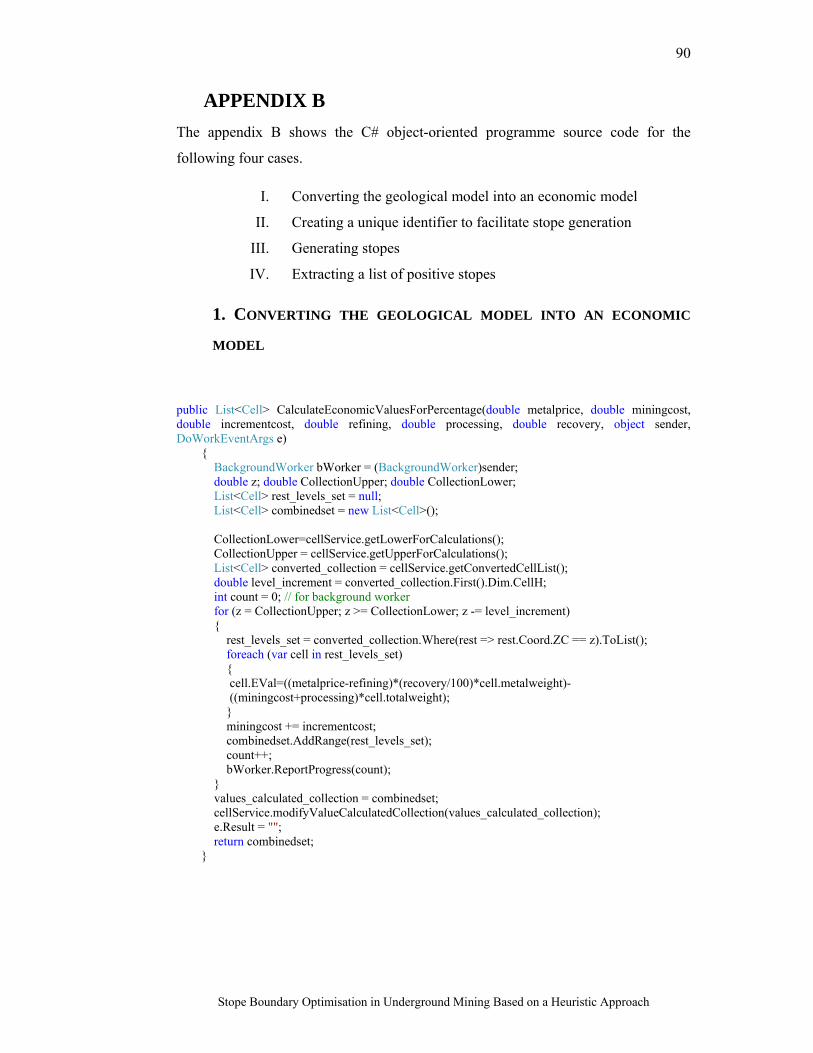
90
Stope Boundary Optimisation in Underground Mining Based on a Heuristic Approach
APPENDIX B
The appendix B shows the C# object-oriented programme source code for the
following four cases.
I. Converting the geological model into an economic model
II. Creating a unique identifier to facilitate stope generation
III. Generating stopes
IV. Extracting a list of positive stopes
1. CONVERTING THE GEOLOGICAL MODEL INTO AN ECONOMIC
MODEL
public List<Cell> CalculateEconomicValuesForPercentage(double metalprice, double miningcost, double incrementcost, double refining, double processing, double recovery, object sender, DoWorkEventArgs e) { BackgroundWorker bWorker = (BackgroundWorker)sender; double z; double CollectionUpper; double CollectionLower; List<Cell> rest_levels_set = null; List<Cell> combinedset = new List<Cell>(); CollectionLower=cellService.getLowerForCalculations(); CollectionUpper = cellService.getUpperForCalculations(); List<Cell> converted_collection = cellService.getConvertedCellList(); double level_increment = converted_collection.First().Dim.CellH; int count = 0; // for background worker for (z = CollectionUpper; z >= CollectionLower; z -= level_increment) { rest_levels_set = converted_collection.Where(rest => rest.Coord.ZC == z).ToList(); foreach (var cell in rest_levels_set) {
cell.EVal=((metalprice-refining)*(recovery/100)*cell.metalweight)- ((miningcost+processing)*cell.totalweight);
} miningcost += incrementcost; combinedset.AddRange(rest_levels_set); count++; bWorker.ReportProgress(count); } values_calculated_collection = combinedset; cellService.modifyValueCalculatedCollection(values_calculated_collection); e.Result = ""; return combinedset; }
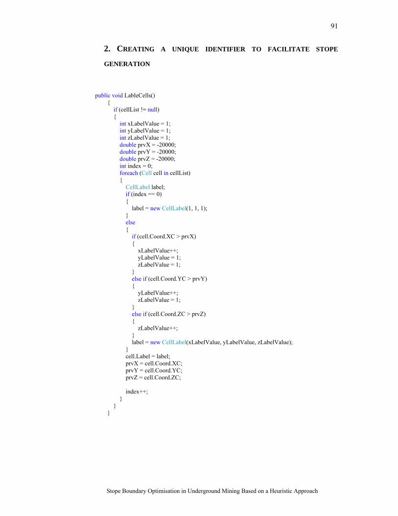
91
Stope Boundary Optimisation in Underground Mining Based on a Heuristic Approach
2. CREATING A UNIQUE IDENTIFIER TO FACILITATE STOPE
GENERATION
public void LableCells() { if (cellList != null) { int xLabelValue = 1; int yLabelValue = 1; int zLabelValue = 1; double prvX = -20000; double prvY = -20000; double prvZ = -20000; int index = 0; foreach (Cell cell in cellList) { CellLabel label; if (index == 0) { label = new CellLabel(1, 1, 1); } else { if (cell.Coord.XC > prvX) { xLabelValue++; yLabelValue = 1; zLabelValue = 1; } else if (cell.Coord.YC > prvY) { yLabelValue++; zLabelValue = 1; } else if (cell.Coord.ZC > prvZ) { zLabelValue++; } label = new CellLabel(xLabelValue, yLabelValue, zLabelValue); } cell.Label = label; prvX = cell.Coord.XC; prvY = cell.Coord.YC; prvZ = cell.Coord.ZC; index++; } } }
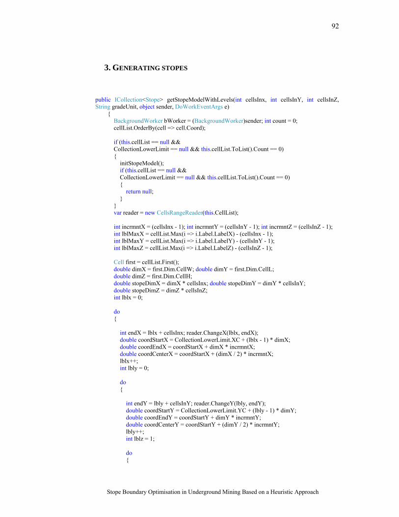
92
Stope Boundary Optimisation in Underground Mining Based on a Heuristic Approach
3. GENERATING STOPES
public ICollection<Stope> getStopeModelWithLevels(int cellsInx, int cellsInY, int cellsInZ, String gradeUnit, object sender, DoWorkEventArgs e) { BackgroundWorker bWorker = (BackgroundWorker)sender; int count = 0; cellList.OrderBy(cell => cell.Coord); if (this.cellList == null && CollectionLowerLimit == null && this.cellList.ToList().Count == 0) { initStopeModel(); if (this.cellList == null && CollectionLowerLimit == null && this.cellList.ToList().Count == 0) { return null; } } var reader = new CellsRangeReader(this.CellList); int incrmntX = (cellsInx - 1); int incrmntY = (cellsInY - 1); int incrmntZ = (cellsInZ - 1); int lblMaxX = cellList.Max(i => i.Label.LabelX) - (cellsInx - 1); int lblMaxY = cellList.Max(i => i.Label.LabelY) - (cellsInY - 1); int lblMaxZ = cellList.Max(i => i.Label.LabelZ) - (cellsInZ - 1); Cell first = cellList.First(); double dimX = first.Dim.CellW; double dimY = first.Dim.CellL; double dimZ = first.Dim.CellH; double stopeDimX = dimX * cellsInx; double stopeDimY = dimY * cellsInY; double stopeDimZ = dimZ * cellsInZ; int lblx = 0; do { int endX = lblx + cellsInx; reader.ChangeX(lblx, endX); double coordStartX = CollectionLowerLimit.XC + (lblx - 1) * dimX; double coordEndX = coordStartX + dimX * incrmntX; double coordCenterX = coordStartX + (dimX / 2) * incrmntX; lblx++; int lbly = 0; do { int endY = lbly + cellsInY; reader.ChangeY(lbly, endY); double coordStartY = CollectionLowerLimit.YC + (lbly - 1) * dimY; double coordEndY = coordStartY + dimY * incrmntY; double coordCenterY = coordStartY + (dimY / 2) * incrmntY; lbly++; int lblz = 1; do {
93
Stope Boundary Optimisation in Underground Mining Based on a Heuristic Approach
int endZ = lblz + cellsInZ; reader.ChangeZ(lblz, endZ); double coordStartZ = CollectionLowerLimit.ZC + (lblz - 1) * dimZ; double coordEndZ = coordStartZ + dimZ * incrmntZ; double coordCenterZ = coordStartZ + (dimZ / 2) * incrmntZ; lblz += cellsInZ; double EVal = 0; double metalweight = 0; double totalweight = 0; double density = 0; int TotalCellsInAStope = cellsInx * cellsInY * cellsInZ; if (reader.GetCells().Count() == TotalCellsInAStope) { foreach (Cell cell in reader.GetCells()) { EVal += cell.EVal; metalweight += cell.metalweight; totalweight += cell.totalweight; density += cell.density ?? 0; } Stope newStope = new Stope(); newStope.stopeEVal = EVal; newStope.metalweight = metalweight; newStope.totalweight = totalweight; newStope.density = density / TotalCellsInAStope; if (gradeUnit == "Grade- %") { newStope.grade = (metalweight / totalweight) * 100; } else if (gradeUnit == "Grade- g/t") { newStope.grade = (metalweight / totalweight) * 100; } newStope.Coord = new Coord(coordStartX, coordStartY, coordStartZ); newStope.EndCordinates = new Coord(coordEndX, coordEndY, coordEndZ); newStope.CenterCordinates = new Coord(coordCenterX, coordCenterY, coordCenterZ); newStope.Dim = new Dim(stopeDimX, stopeDimY, stopeDimZ); this.stopeList.Add(newStope); count++; if (count % 1000 == 0) { bWorker.ReportProgress(count); } } } while (lblz <= lblMaxZ); } while (lbly <= lblMaxY); } while (lblx <= lblMaxX); e.Result = ""; return this.stopeList; }
94
Stope Boundary Optimisation in Underground Mining Based on a Heuristic Approach
4. EXTRACTING A LIST OF POSITIVE STOPES
public int positvestopes_count = 0; public Boolean UpdatePositiveStopes() { cellService.removePositiveStopes(); List<Stope> positivestopes = cellService.extractPositiveStopes(); positvestopes_count = positivestopes.Count; if (positivestopes != null && positivestopes.Count > 0) { foreach (Stope stope in positivestopes) { cellService.modifyPositiveStopes(stope); } return true; } else { return false; } }