Statistics 222, Spatial Statistics.

Outline for the day:

1. Poisson process, continued.

2. Mixed Poisson process.

3. Compound Poisson process

4. Poisson cluster process.

5. Cox process.

6. Gibbs processes.

7. Matern processes.

8. Examples and code.

1. Poisson processes.

Last week we discussed Poisson processes.

If N is a simple point process with conditional intensity l, where l does not depend on what points have occurred previously, then N is a Poisson process.

For such a process, for any set B, N(B) has a Poisson distribution. P(N(B) = k) = e-A Ak / k! , for k = 0, 1, 2, ..., where A = ∫B l(t,x,y) dtdxdy, and with the convention 0! = 1.The mean of N(B) is A and the varianceis also A. E(N(B)2) = A2 + A.

We will now discuss a few extensions of Poisson processes.

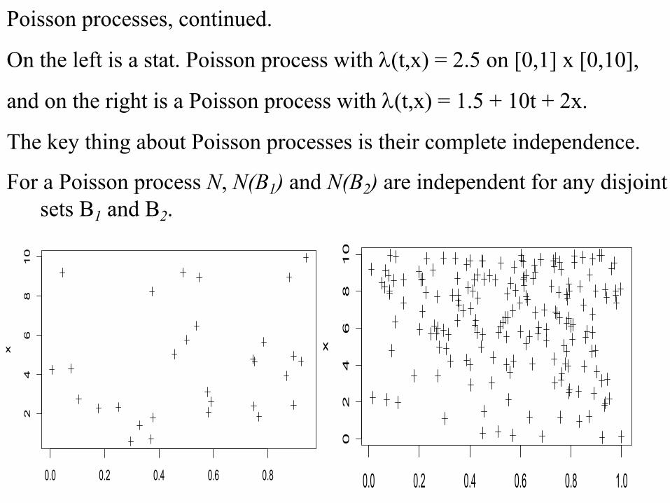
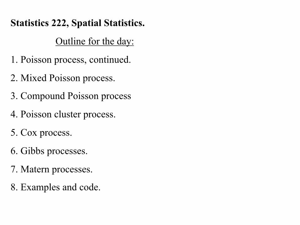
Poisson processes, continued.

On the left is a stat. Poisson process with l(t,x) = 2.5 on [0,1] x [0,10],

and on the right is a Poisson process with l(t,x) = 1.5 + 10t + 2x.

The key thing about Poisson processes is their complete independence.

For a Poisson process N, N(B1) and N(B2) are independent for any disjoint sets B1 and B2.

0.0 0.2 0.4 0.6 0.8

24

68

10

t

x

0.0 0.2 0.4 0.6 0.8 1.0

02

46

810

t

x

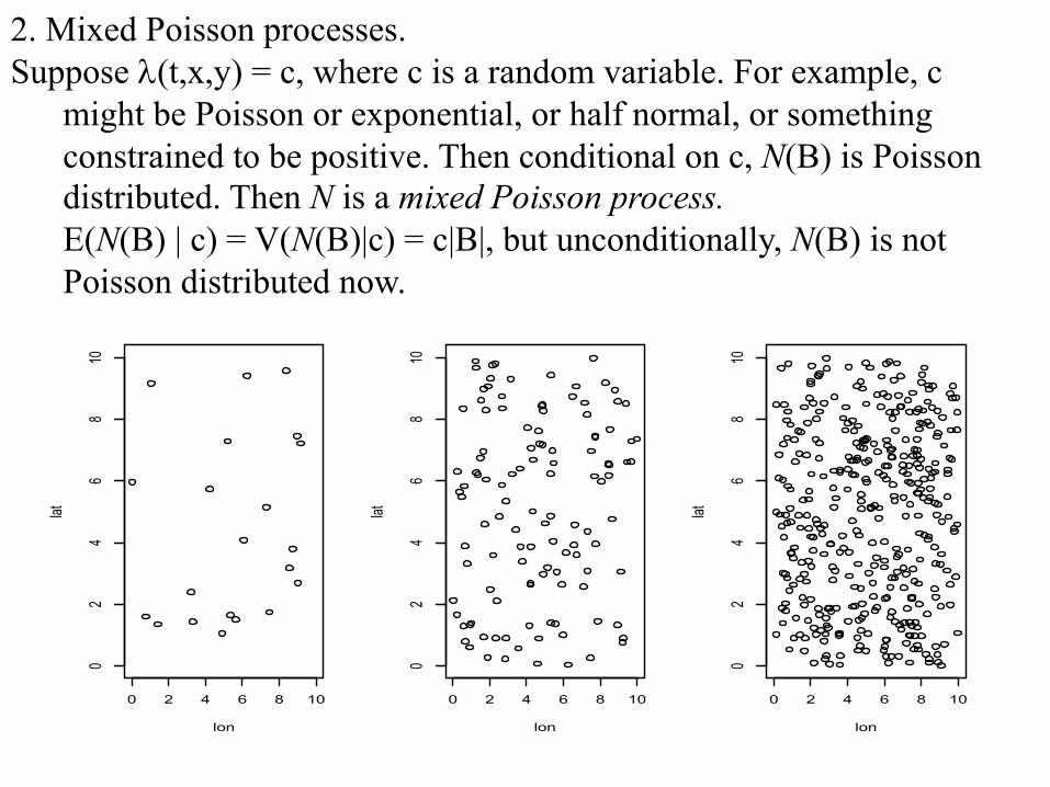
2. Mixed Poisson processes. Suppose l(t,x,y) = c, where c is a random variable. For example, c

might be Poisson or exponential, or half normal, or something constrained to be positive. Then conditional on c, N(B) is Poisson distributed. Then N is a mixed Poisson process. E(N(B) | c) = V(N(B)|c) = c|B|, but unconditionally, N(B) is not Poisson distributed now.

0 2 4 6 8 10

02

46

810

lon

lat

0 2 4 6 8 10

02

46

810

lon

lat

0 2 4 6 8 10

02

46

810

lon

lat

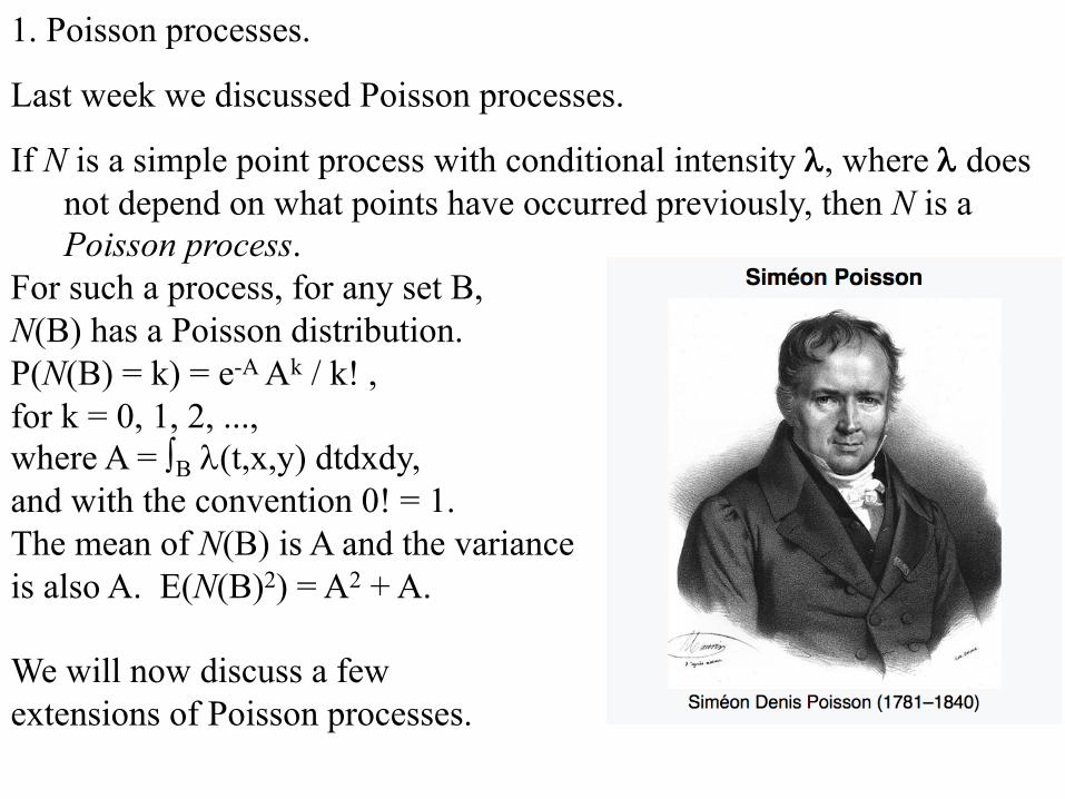
2. Mixed Poisson processes. Suppose l(t,x,y) = c, where c is a random variable. For example, c

might be Poisson or exponential, or half normal, or something constrained to be positive. Then conditional on c, N(B) is Poisson distributed. Then N is a mixed Poisson process. E(N(B) | c) = V(N(B)|c) = c|B|, but unconditionally, N(B) is not Poisson distributed now. If we imagine simulating the process repeatedly, each time with a different draw of c, then the distribution of N(B) will not be Poisson. N(B) will typically be overdispersed relative to the Poisson process, i.e. will have higher variance.

E(N(B)) = ∫ E(N(B)|c) f(c)dc = ∫ c|B| f(c)dc = |B|E(c).E(N(B)2) = ∫ E(N(B)|c)2 f(c) dc = ∫ [c2|B|2 + c|B|] f(c) dc = |B|2 E(c2) + |B|E(c), so V(N(B)) = |B|2 E(c2) + |B|E(c) - |B|2 [E(c)]2 = E(N(B)) + |B|2 V(c). So, V(N(B)) ≥ E(N(B)).

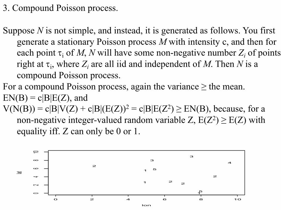
3. Compound Poisson process.

Suppose N is not simple, and instead, it is generated as follows. You first generate a stationary Poisson process M with intensity c, and then for each point ti of M, N will have some non-negative number Zi of points right at ti, where Zi are all iid and independent of M. Then N is a compound Poisson process.

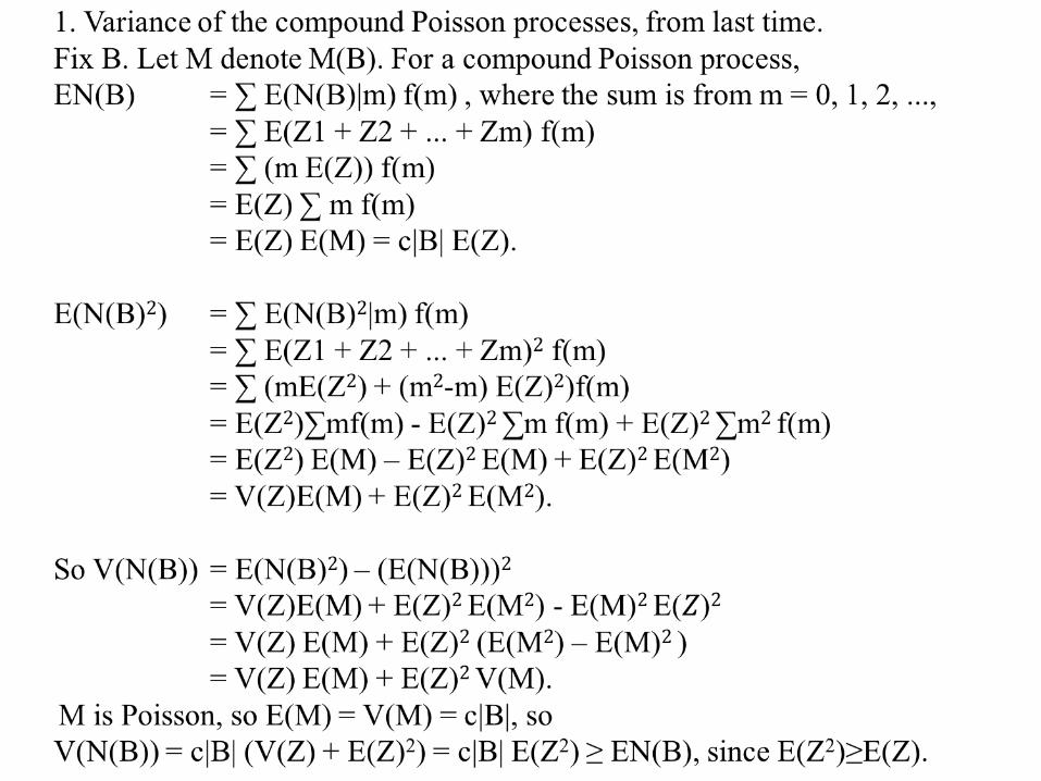
For a compound Poisson process, again the variance ≥ the mean. EN(B) = c|B|E(Z), and V(N(B)) = c|B|V(Z) + c|B|(E(Z))2 = c|B|E(Z2) ≥ EN(B), because, for a

non-negative integer-valued random variable Z, E(Z2) ≥ E(Z) with equality iff. Z can only be 0 or 1.

0 2 4 6 8 10

02

46

810

lon

lat

51

4

2

3

2

1

2

3

2

5

1

3. Variance of the compound Poisson process. Fix B. Let M denote M(B). For a compound Poisson process, EN(B) = c|B| E(Z). E(N(B)2) = V(Z) E(M) + (E(Z))2 E(M2). So V(N(B)) = V(Z) E(M) + E(Z)2 V(M). M is Poisson, so E(M) = V(M) = c|B|, so V(N(B)) = c|B| (V(Z) + E(Z)2 ) = c|B| E(Z2) ≥ EN(B), since E(Z2) ≥ E(Z) because Z is nonnegative integer valued.

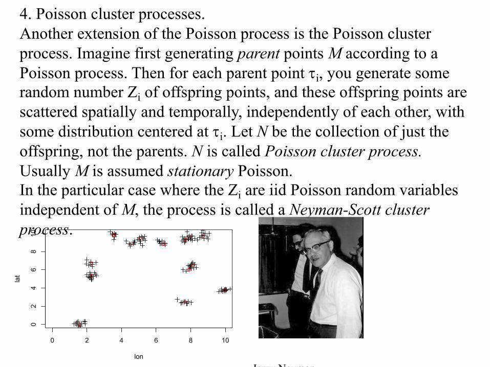
4. Poisson cluster processes. Another extension of the Poisson process is the Poisson cluster process. Imagine first generating parent points M according to a Poisson process. Then for each parent point ti, you generate some random number Zi of offspring points, and these offspring points are scattered spatially and temporally, independently of each other, with some distribution centered at ti. Let N be the collection of just the offspring, not the parents. N is called Poisson cluster process. Usually M is assumed stationary Poisson. In the particular case where the Zi are iid Poisson random variables independent of M, the process is called a Neyman-Scott cluster process.

Jerzy Neyman

0 2 4 6 8 10

02

46

810

lon

lat

5. Cox process.

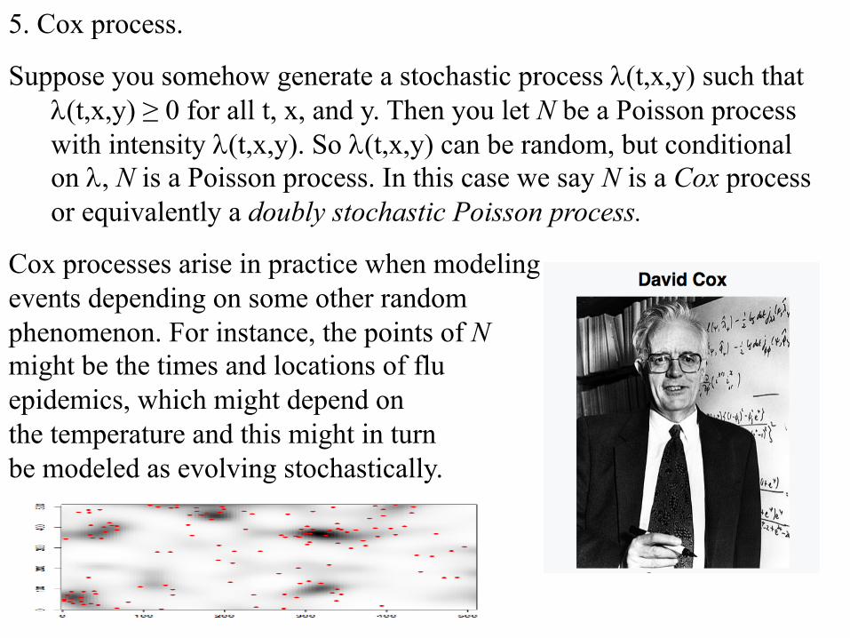
Suppose you somehow generate a stochastic process l(t,x,y) such that l(t,x,y) ≥ 0 for all t, x, and y. Then you let N be a Poisson process with intensity l(t,x,y). So l(t,x,y) can be random, but conditional on l, N is a Poisson process. In this case we say N is a Cox process or equivalently a doubly stochastic Poisson process.

Cox processes arise in practice when modelingevents depending on some other randomphenomenon. For instance, the points of Nmight be the times and locations of fluepidemics, which might depend on the temperature and this might in turn be modeled as evolving stochastically.

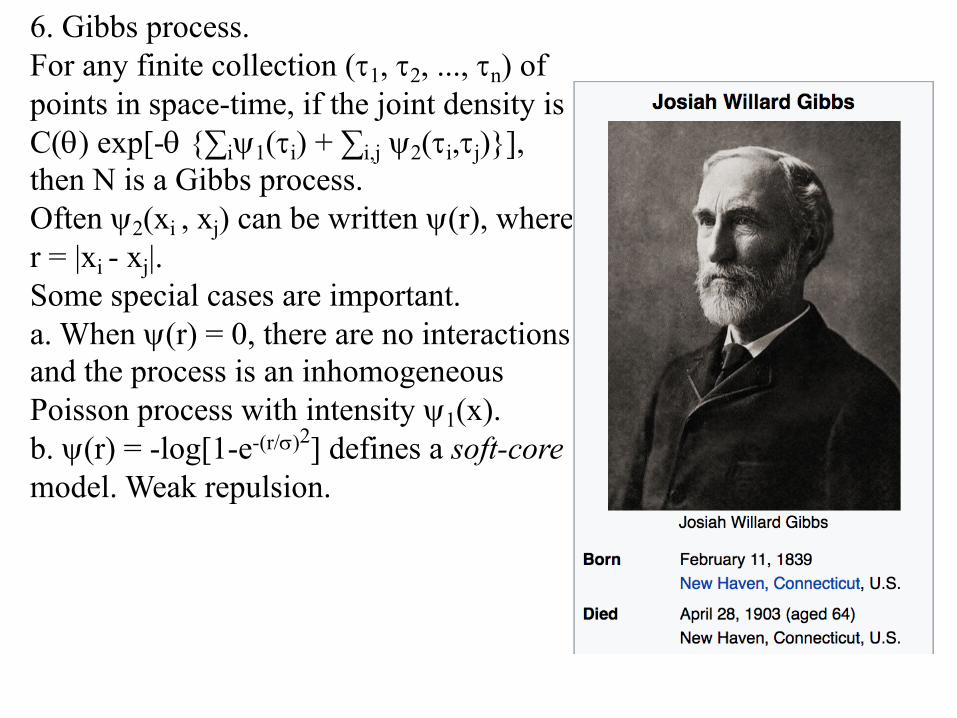
6. Gibbs process. For any finite collection (t1, t2, ..., tn) of points in space-time, if the joint density is C(q) exp[-q {∑iy1(ti) + ∑i,j y2(ti,tj)}], then N is a Gibbs process. Often y2(xi , xj) can be written y(r), where r = |xi - xj|.Some special cases are important. a. When y(r) = 0, there are no interactions, and the process is an inhomogeneous Poisson process with intensity y1(x). b. y(r) = -log[1-e-(r/s)2] defines a soft-coremodel. Weak repulsion.

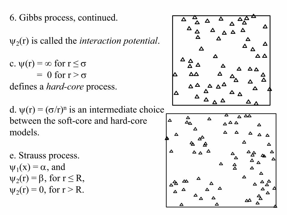
6. Gibbs process, continued.

y2(r) is called the interaction potential.

c. y(r) = ∞ for r ≤ s= 0 for r > s

defines a hard-core process.

d. y(r) = (s/r)n is an intermediate choice between the soft-core and hard-core models.

e. Strauss process. y1(x) = a, and y2(r) = b, for r ≤ R,y2(r) = 0, for r > R.

z

z

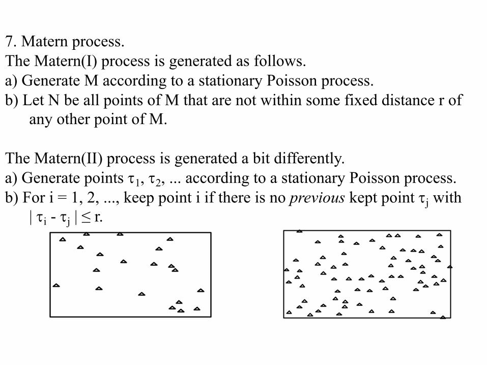
7. Matern process. The Matern(I) process is generated as follows. a) Generate M according to a stationary Poisson process. b) Let N be all points of M that are not within some fixed distance r of

any other point of M.

The Matern(II) process is generated a bit differently.a) Generate points t1, t2, ... according to a stationary Poisson process.b) For i = 1, 2, ..., keep point i if there is no previous kept point tj with

| ti - tj | ≤ r. z z

Exercises.

1. A mixed Poisson process is a Cox process where

a. l = E(l) in every realization.

b. l(t,x,y) = l(t',x',y'), for any locations (t,x,y) and (t',x',y').

c. The cluster sizes are Poisson distributed with mean l.

d. l = 1.

Exercises.

1. A mixed Poisson process is a Cox process where

a. l = E(l) in every realization.

b. l(t,x,y) = l(t',x',y'), for any locations (t,x,y) and (t',x',y').

c. The cluster sizes are Poisson distributed with mean l.

d. l = 1.

a. means l is a constant, so N is a stationary Poisson process. d. Also defines a stationary Poisson process, with rate 1.

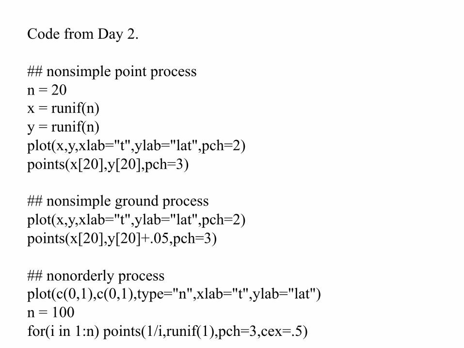
Code from Day 2.

## nonsimple point process n = 20x = runif(n)y = runif(n)plot(x,y,xlab="t",ylab="lat",pch=2)points(x[20],y[20],pch=3)

## nonsimple ground process plot(x,y,xlab="t",ylab="lat",pch=2)points(x[20],y[20]+.05,pch=3)

## nonorderly processplot(c(0,1),c(0,1),type="n",xlab="t",ylab="lat")n = 100for(i in 1:n) points(1/i,runif(1),pch=3,cex=.5)

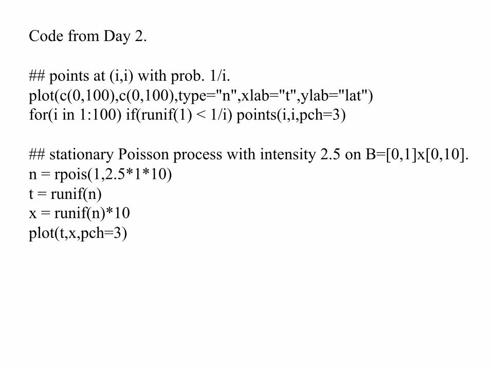
Code from Day 2.

## points at (i,i) with prob. 1/i. plot(c(0,100),c(0,100),type="n",xlab="t",ylab="lat")for(i in 1:100) if(runif(1) < 1/i) points(i,i,pch=3)

## stationary Poisson process with intensity 2.5 on B=[0,1]x[0,10].n = rpois(1,2.5*1*10)t = runif(n)x = runif(n)*10plot(t,x,pch=3)

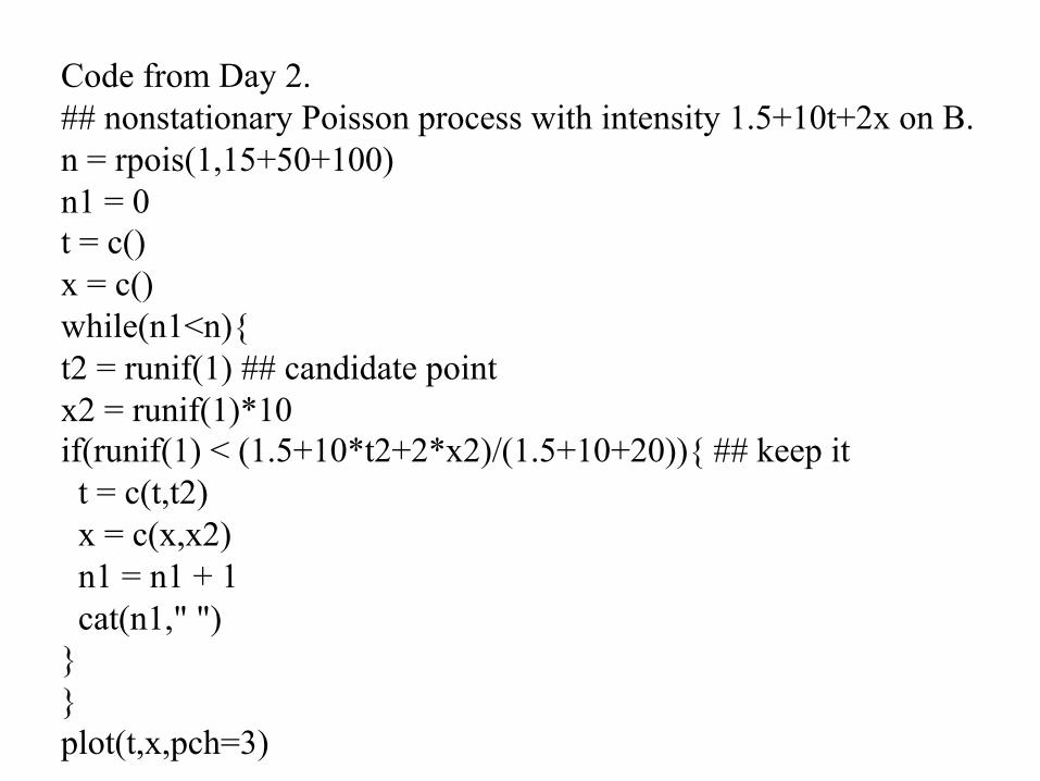
Code from Day 2. ## nonstationary Poisson process with intensity 1.5+10t+2x on B.n = rpois(1,15+50+100)n1 = 0t = c()x = c()while(n1<n){t2 = runif(1) ## candidate pointx2 = runif(1)*10if(runif(1) < (1.5+10*t2+2*x2)/(1.5+10+20)){ ## keep itt = c(t,t2)x = c(x,x2)n1 = n1 + 1cat(n1," ")

}}plot(t,x,pch=3)

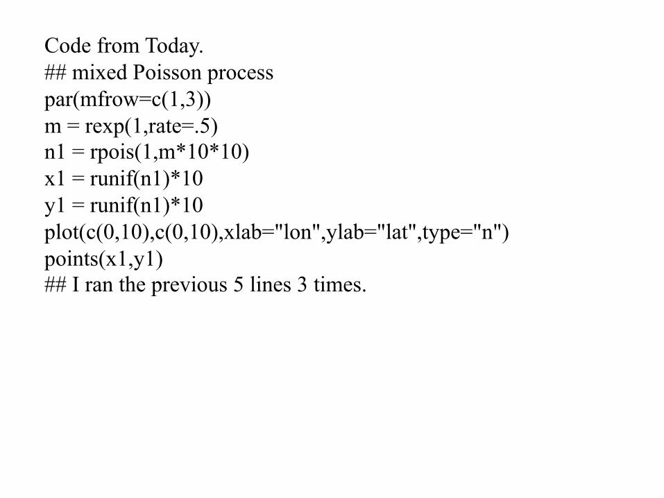
Code from Today. ## mixed Poisson processpar(mfrow=c(1,3))m = rexp(1,rate=.5)n1 = rpois(1,m*10*10)x1 = runif(n1)*10y1 = runif(n1)*10plot(c(0,10),c(0,10),xlab="lon",ylab="lat",type="n")points(x1,y1) ## I ran the previous 5 lines 3 times.

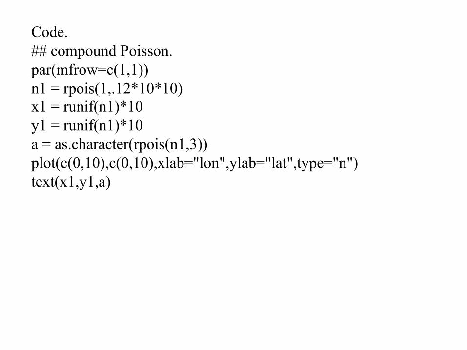
Code.## compound Poisson. par(mfrow=c(1,1))n1 = rpois(1,.12*10*10)x1 = runif(n1)*10y1 = runif(n1)*10a = as.character(rpois(n1,3))plot(c(0,10),c(0,10),xlab="lon",ylab="lat",type="n")text(x1,y1,a)

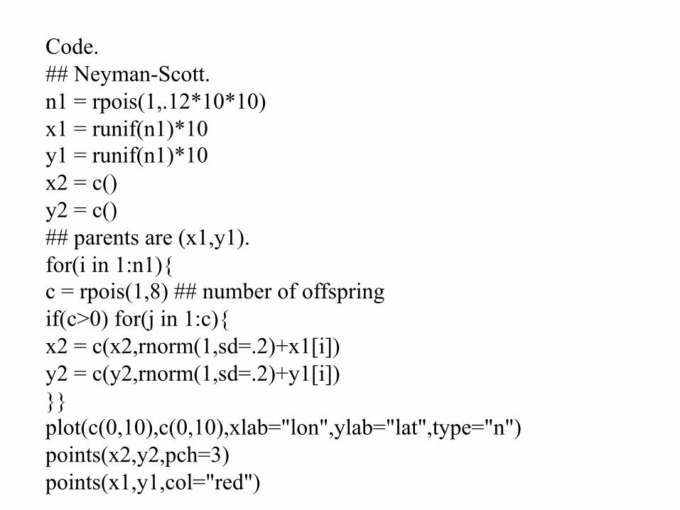
Code.## Neyman-Scott. n1 = rpois(1,.12*10*10)x1 = runif(n1)*10y1 = runif(n1)*10x2 = c()y2 = c()## parents are (x1,y1). for(i in 1:n1){ c = rpois(1,8) ## number of offspringif(c>0) for(j in 1:c){x2 = c(x2,rnorm(1,sd=.2)+x1[i])y2 = c(y2,rnorm(1,sd=.2)+y1[i])}}plot(c(0,10),c(0,10),xlab="lon",ylab="lat",type="n")points(x2,y2,pch=3)points(x1,y1,col="red")