Embed Size (px)
Citation preview


Theory of SpatialStatistics
A Concise Introduction

Theory of SpatialStatistics
A Concise Introduction
M.N.M. van Lieshout
CRC PressTaylor & Francis Group6000 Broken Sound Parkway NW, Suite 300Boca Raton, FL 33487-2742
⃝c 2019 by Taylor & Francis Group, LLCCRC Press is an imprint of Taylor & Francis Group, an Informa business
No claim to original U.S. Government works
Printed on acid-free paper
International Standard Book Number-13: 978-0-367-14642-9 (Hardback)978-0-367-14639-9 (Paperback)
This book contains information obtained from authentic and highly regarded sources. Rea-sonable efforts have been made to publish reliable data and information, but the authorand publisher cannot assume responsibility for the validity of all materials or the conse-quences of their use. The authors and publishers have attempted to trace the copyrightholders of all material reproduced in this publication and apologize to copyright holders ifpermission to publish in this form has not been obtained. If any copyright material has notbeen acknowledged please write and let us know so we may rectify in any future reprint.
Except as permitted under U.S. Copyright Law, no part of this book may be reprinted,reproduced, transmitted, or utilized in any form by any electronic, mechanical, or othermeans, now known or hereafter invented, including photocopying, microfilming, and record-ing, or in any information storage or retrieval system, without written permission from thepublishers.
For permission to photocopy or use material electronically from this work, please accesswww.copyright.com (http://www.copyright.com/) or contact the Copyright Clearance Cen-ter, Inc. (CCC), 222 Rosewood Drive, Danvers, MA 01923, 978-750-8400. CCC is a not-for-profit organization that provides licenses and registration for a variety of users. Fororganizations that have been granted a photocopy license by the CCC, a separate systemof payment has been arranged.
Trademark Notice: Product or corporate names may be trademarks or registered trade-marks, and are used only for identification and explanation without intent to infringe.
Library of Congress Cataloging-in-Publication Data
Names: van Lieshout, M. N. M., author.Title: Theory of spatial statistics : a concise introduction / by M.N.M. vanLieshout.Description: Boca Raton, Florida : CRC Press, 2019. | Includes bibliograph-ical references and index.Identifiers: LCCN 2018052975| ISBN 9780367146429 (hardback : alk.paper) | ISBN 9780367146399 (pbk. : alk. paper) | ISBN 9780429052866(e-book)Subjects: LCSH: Spatial analysis (Statistics)Classification: LCC QA278.2 .V36 2019 | DDC 519.5/35- -dc23LC record available at https://lccn.loc.gov/2018052975
Visit the Taylor & Francis Web site athttp://www.taylorandfrancis.com
and the CRC Press Web site athttp://www.crcpress.com

To Catharina Johanna Schoenmakers.

Contents
Preface xi
Author xiii
Chapter 1 ! Introduction 1
1.1 GRIDDED DATA 11.2 AREAL UNIT DATA 31.3 MAPPED POINT PATTERN DATA 41.4 PLAN OF THE BOOK 6
Chapter 2 ! Random field modelling and interpolation 9
2.1 RANDOM FIELDS 92.2 GAUSSIAN RANDOM FIELDS 112.3 STATIONARITY CONCEPTS 132.4 CONSTRUCTION OF COVARIANCE FUNCTIONS 162.5 PROOF OF BOCHNER’S THEOREM 202.6 THE SEMI-VARIOGRAM 232.7 SIMPLE KRIGING 262.8 BAYES ESTIMATOR 282.9 ORDINARY KRIGING 292.10 UNIVERSAL KRIGING 322.11 WORKED EXAMPLES WITH R 342.12 EXERCISES 422.13 POINTERS TO THE LITERATURE 46
vii

viii ! Contents
Chapter 3 ! Models and inference for areal unit data 49
3.1 DISCRETE RANDOM FIELDS 493.2 GAUSSIAN AUTOREGRESSION MODELS 523.3 GIBBS STATES 553.4 MARKOV RANDOM FIELDS 593.5 INFERENCE FOR AREAL UNIT MODELS 623.6 MARKOV CHAIN MONTE CARLO SIMULATION 673.7 HIERARCHICAL MODELLING 70
3.7.1 Image segmentation 703.7.2 Disease mapping 733.7.3 Synthesis 75
3.8 WORKED EXAMPLES WITH R 763.9 EXERCISES 843.10 POINTERS TO THE LITERATURE 88
Chapter 4 ! Spatial point processes 93
4.1 POINT PROCESSES ON EUCLIDEAN SPACES 934.2 THE POISSON PROCESS 964.3 MOMENT MEASURES 984.4 STATIONARITY CONCEPTS AND PRODUCT
DENSITIES 1004.5 FINITE POINT PROCESSES 1044.6 THE PAPANGELOU CONDITIONAL INTENSITY 1084.7 MARKOV POINT PROCESSES 1104.8 LIKELIHOOD INFERENCE FOR POISSON
PROCESSES 1124.9 INFERENCE FOR FINITE POINT PROCESSES 1144.10 COX PROCESSES 117
4.10.1 Cluster processes 1184.10.2 Log-Gaussian Cox processes 1204.10.3 Minimum contrast estimation 121

Contents ! ix
4.11 HIERARCHICAL MODELLING 1234.12 WORKED EXAMPLES WITH R 1264.13 EXERCISES 1344.14 POINTERS TO THE LITERATURE 137
Appendix: Solutions to theoretical exercises 143
Index 167

Preface
Today, much information reaches us in graphical form. From a math-ematical point of view, such data may be divided into various classes,each having its own salient characteristics. For instance, in classical geo-statistics, some spatially varying variable is observed at a given numberof fixed locations and one is interested in its value at locations whereit was not observed. One might think of the prediction of ore contentin the soil based on measurements at some conveniently placed bore-holes or the construction of air pollution maps based on gauge data.In other cases, due to technical constraints or for privacy reasons, datais collected in aggregated form as region counts or as a discrete image.Typical examples include satellite imagery, tomographic scans, diseasemaps or yields in agricultural field trials. In this case, the objective isoften spatial smoothing or sharpening rather than prediction. Finally,data may consist of a set of objects or phenomena tied to random spa-tial locations and the prime interest is in the geometrical arrangementof the set, for instance in the study of earthquakes or of cellular patternsseen under a microscope.
The statistical analysis of spatial data merits treatment as a separatetopic, as it is different from ‘classical’ statistical data in a number ofaspects. Typically, only a single observation is available, so that artificialreplication in the form of an appropriate stationarity assumption is calledfor. Also the size of images, or the number of objects in a spatial pattern,is typically large and, moreover, there may be interactions at variousscales. Hence a conditional or hierarchical specification is useful, oftenin combination with Monte Carlo methods.
This book will describe the mathematical foundations for each ofthe data classes mentioned above, present some models and discuss sta-tistical inference. Each chapter first presents the theory which is thenapplied to illustrative examples using an open source R-package, listssome exercises and concludes with pointers to the literature. The pre-requisites consist of maturity in probability and statistics at the levelexpected of a graduate student in mathematics, engineering or statistics.
xi

xii ! Preface
Indeed, the contents grew out of lectures in the Dutch graduate school‘Mastermath’ and are suitable for a semester long introduction. Thosewishing to learn more are referred to the excellent monographs by Cressie(Wiley, 2015), by Banerjee, Carlin and Gelfand (CRC, 2004) and byGaetan and Guyon (Springer, 2010) or to the exhaustive Handbook ofSpatial Statistics (CRC, 2010).
In closing, I would like to express my gratitude to the studentswho attended my ‘Mastermath’ courses for useful feedback, to the staffat Taylor and Francis, especially to Rob Calver, for their support, tothree anonymous reviewers for constructive suggestions and to ChristophHofer–Temmel for a careful reading of the manuscript.
Marie-Colette van LieshoutAmsterdam, September 2018

Author
M.N.M. van Lieshout is a senior researcher at the Centre for Mathe-matics and Computer Science (CWI) in Amsterdam, The Netherlands,and holds a chair in spatial stochastics at the University of Twente.
xiii

C H A P T E R 1
Introduction
The topic of these lecture notes is modelling and inference for spatialdata. Such data, by definition, involve measurements at some spatiallocations, but can take many forms depending on the stochastic mech-anism that generated the data, on the type of measurement and on thechoice of the spatial locations.
Ideally, the feature of interest is measured at every location in someappropriate region, usually a bounded subset of the plane. From a math-ematical point of view, such a situation can be described by a randomfield indexed by the region. In practice, however, it is not possible toconsider infinitely many locations. Additionally, there may be physical,administrative, social or economic reasons for limiting the number ofsampling locations or for storing measurements in aggregated form overareal units. The locations may even be random, so that, in mathematicalterms, they constitute a point process.
In the next three sections, we will present some typical examplesto motivate the more mathematical treatment in subsequent chapters.Suggestions for statistical inference will also be given, but note that theseshould be taken as an indication. Indeed, any pertinent analysis shouldtake into account the data collection process, the specific context and thescientific question or goal that prompted data collection in the first place.
1.1 GRIDDED DATA
Figure 1.1 shows 208 coal ash core samples collected on a grid in theRobena Mine in Greene County, Pennsylvania. The diameters of thediscs are proportional to the percentage of coal ash at the sampled loca-tions. The data can be found in a report by Gomez and Hazen [1] and
1

2 ! Introduction
78.969.78510.56717.61
Figure 1.1 Percentage of coal ash sampled on a grid in the Robena Minein Greene County, Pennsylvania.
were prepared for R by E. Pebesma using a digital version at a websitemaintained by D. Zimmerman.
A mining engineer might be interested in knowing basic summarystatistics, including the first and second moments of the sample. Next,with model building in mind, he could ask himself whether the datacould have come from a normal distribution, possibly after discardingsome outliers, and if not, whether they are multi-modal or skewed. Suchquestions could be addressed by elementary tools including histograms,quantiles, boxplots and Q-Q plots.
On a higher conceptual level, the mining company could also beinterested in local outliers, measured percentages that are markedly dif-ferent from those around them, or in trends that could indicate goodplaces to concentrate future mining efforts. Indications of these can befound by applying the elementary statistics across rows or columns. Forinstance, consideration of the mean across columns suggests that thereis a decreasing trend in the percentage of coal ash from left to right. It

Areal unit data ! 3
would be of interest to quantify how strongly correlated measurementsat adjacent sampling locations are too.
Another striking feature of Figure 1.1 is that there are holes in thesampling grid, for example in the seventh row from above and in thesixth one from below. Therefore, when the mining engineer has found andvalidated a reasonable model that accounts for both the global trendsand the local dependencies in the data, he could proceed to try and fillin the gaps, in other words, to estimate the percentage of coal ash atmissing grid points based on the sampled percentages. Such a spatialinterpolation procedure is called kriging in honour of the South-Africanstatistician and mining engineer D.G. Krige, one of the pioneers of whatis now known as geostatistics.
1.2 AREAL UNIT DATA
The top-most panel of Figure 1.2 shows a graphical representation ofthe total number of deaths from Sudden Infant Death Syndrome (SIDS)in 1974 for each of the 100 counties in North Carolina. These data werecollected by the state’s public health statistics branch and analysed in[2]. More precisely, the counts were binned in five colour-coded intervals,where darker colours correspond to higher counts.
From the picture it is clear that the centroids of the counties do notlie on a regular grid. The sizes and shapes of the counties vary and canbe quite irregular. Moreover, the recorded counts are not tied to a pre-cise location but tallied up county-wise. This kind of accumulation overadministrative units is usual for privacy-sensitive data in, for instance,the crime or public health domains.
A public health official could be interested in spatial patterns. Indeed,the original research question in [2] was whether or not there are clustersof counties with a high incidence of SIDS. However, death counts bythemselves are quite meaningless without an indication of the populationat risk. For this purpose, Symons, Grimson and Yuan [3] asked the NorthCarolina public health statistics branch for the counts of live births ineach county during the same year 1974. These are shown in the lowerpanel of Figure 1.2.
Presented with the two pictures, our public health official might lookfor areas where the SIDS counts are higher than what would be expectedbased on the number of live births in the area. Such areas would beprime targets for an information campaign or a quest for factors specificto those areas that could explain the outlier. For the data at hand, whencomparing counties at the north-east and the north-west with similar

4 ! Introduction
Figure 1.2 Numbers of cases of Sudden Infant Death Syndrome (top)and live births (bottom) during 1974 accumulated per county in NorthCarolina. The death counts are binned in five classes with breaks at5, 10, 15 and 20, the live birth counts in six classes with breaks at 1000,2000, 3000, 4000 and 5000. Darker colours correspond to higher counts.
birth numbers, it is clear that there is a higher SIDS rate in the north-east. Note that there are also counties in the centre of the state with ahigh number of births but a rather low SIDS incidence. Other outlierscan be identified using classic boxplots and quantile techniques on therates of SIDS compared to live births.
Such an analysis, however, ignores the fact that the county bordersare purely administrative and disease patterns are unlikely to follow.Moreover, rates in counties with many births are likely to be more stablethan those with few. On a higher conceptual level, the public healthauthority may therefore wish for a model that explicitly accounts forlarge scale variations in expected rates and their associated variances aswell as for local dependencies between adjacent counties.
1.3 MAPPED POINT PATTERN DATA
Figure 1.3 shows a mapped pattern consisting of 3, 605 Beilschmiediatrees in a rectangular stand of tropical rain forest at Barro Colorado

Mapped point pattern data ! 5
Figure 1.3 Top: positions of Beilschmiedia trees in a 1,000 by 500 metrestand in Barro Colorado Island, Panama. Bottom: norm of elevation (inmetres) gradient in the stand.
Island, Panama. These data were prepared for R by R. Waagepetersenand taken from a larger data set described in [4].
We will only be interested in maps where the mechanism that gener-ated the points is of interest. For instance, since the map of centroids ofthe North Carolina counties discussed in the previous section is purelyartificial and has no bearing on the abundance of SIDS cases, there is nopoint in studying it. For genuine mapped point pattern data, researchquestions tend to focus on the arrangement of the points, in particular,on trends and interactions.
Returning to Figure 1.3, it is clear at first glance that the trees arenot distributed over the plot in a uniform way. Rather, they seem tobe concentrated in specific regions. Possible explanations could includelocal differences in soil quality or the availability of nutrients, differencesin the terrain, or traces of a planting scheme. To quantify and test non-homogeneity, the forester may use quadrats, that is, a partition of thestand in disjoint spatial bins, and apply classical statistical dispersiontests to the quadrat counts. It might also be of interest to test whetherthe counts follow a Poisson distribution.

6 ! Introduction
Since Barro Colorado island has been studied extensively over thepast century, a lot is known about the terrain. The image in the lower-most panel of Figure 1.3 displays the norm of the elevation gradient.Visually, it seems that a steep gradient aligns well with a high treeintensity, a correlation that the forester may be interested in quantifyingby means of a spatial generalised linear regression model.
The steepness of the terrain is only one factor in explaining themapped pattern. A cluster in the left part of the stand, for example,is rich in trees, even though the terrain there is not steep at all. Addi-tionally, there could be interaction between the trees due to competitionfor nutrients or sunlight or because of seed dispersion patterns that theforester may try to capture in a model.
Finally note that additional measurements might be taken at eachtree location, for example the number of stems, the size of the crown orthe diameter at breast height, but we will not pursue this topic further.
1.4 PLAN OF THE BOOK
Chapter 2 is devoted to gridded data such as the coal ash measurementsdisplayed in Figure 1.1. The mathematical definition of a random field isgiven before specialising to Gaussian random fields. Such random fieldsare convenient to work with since their distribution is fully described bythe mean and covariance functions. Next, various types of stationarityare discussed and shown to be equivalent for Gaussian random fields.The celebrated Bochner theorem provides a spectral representation forcontinuous covariance functions.
The second part of the chapter is dedicated to spatial interpolation.First, the semi-variogram and its empirical counterpart are introducedto quantify the local interaction structure in the data. A simple krigingprocedure is developed that is appropriate when both the mean and thesemi-variogram are known explicitly. It is shown that this procedure re-duces to a Bayes estimator when the random field is Gaussian. In thelast sections of the chapter, the strong assumptions on mean and semi-variogram are relaxed. More precisely, ordinary kriging is the name givento spatial interpolation when the mean is constant but unknown. Uni-versal kriging is apt when explanatory variables are available to definea spatial regression for the mean.
Chapter 3 is concerned with areal unit data such as the infant deathcounts shown in Figure 1.2. Special attention is given to autoregressionmodels, including Gaussian and logistic ones. It is shown that, provided

Plan of the book ! 7
a positivity condition holds, the distribution of such models is fully de-scribed by their local characteristics, that is, by the family of the condi-tional distributions of the measurement at each areal unit given those atother units. When these local characteristics are truly local in the sensethat they depend only on the neighbours of the areal unit of interest,the random field is said to be Markov. Using the theory of Gibbs states,it is proved that the joint probability density of a Markov random fieldcan be factorised in interaction functions on sets of mutual neighbours.
The second part of the chapter is devoted to statistical inference,in particular estimation of the model parameters. First, the maximumlikelihood equations are derived for a Gaussian autoregression model.For most other models, the likelihood is available only up to a parame-ter dependent normalisation constant. Several techniques are discussed,including maximum pseudo-likelihood and Monte Carlo maximum like-lihood estimation. The chapter closes with two examples of hierarchicalmodelling and inference, image segmentation and disease mapping.
The last chapter, Chapter 4, features mapped point pattern datasuch as the map of trees in Figure 1.3. The formal definition of a pointprocess is given before specialising to Poisson processes. These processesare convenient to work with because of the lack of interaction betweentheir points, and the fact that their distribution is fully described by theintensity function. Next, the moment measures and associated productdensities are defined for general point processes, together with their em-pirical counterparts. Various concepts of stationarity are also discussed.
The remainder of the chapter is restricted to finite point processes.Following similar lines as those laid out in Chapter 3, a family of condi-tional distributions is defined on which a Markov property can be basedand a factorisation of the joint probability density in terms of interac-tion functions defined on sets of mutual neighbours is seen to hold. Amaximum likelihood theory is developed for Poisson processes, whilstthe maximum pseudo-likelihood and Monte Carlo maximum likelihoodmethods apply more generally. Minimum contrast techniques can be usedfor point processes, including Cox and cluster processes, for which thelikelihood is intractable. An application to cluster centre detection con-cludes the chapter.
Each chapter also contains worked examples and exercises to illus-trate, complement and bring the theory into practice. In order to makethe book suitable for self-study, solutions to selected exercises are col-lected in an appendix. The chapters close with pointers to the original

8 ! Introduction
sources of the results, in so far as it was possible to trace them, and tomore specialised and elaborate textbooks for further study.
The calculations in this book were done using the R-language, a free,open source implementation of the S programming language created byJ.M. Chambers [5]. R was created in the 1990s by R. Ihaka and R.Gentleman and is being developed by the R Development Core Teamcurrently consisting of some twenty people. For an introduction, we referto [6]. An attractive feature of the R-project is that it comes with a greatmany state of the art packages contributed by prominent researchers.The current list of packages is available at the site cran.r-project.org.A bit of a warning, though. Packages come with absolutely no warranty!Of course, it is also possible to write one’s own functions and to loadC-code.
REFERENCES
[1] M. Gomez and K. Hazen (1970). Evaluating sulfur and ash distribution in coalseams by statistical response surface regression analysis. U.S. Bureau ofMines Report RI 7377.
[2] D. Atkinson (1978). Epidemiology of sudden infant death in North Car-olina: Do cases tend to cluster? North Carolina Department of HumanResources, Division of Health Services Public Health Statistics BranchStudy 16.
[3] M.J. Symons, R.C. Grimson and Y.C. Yuan (1983). Clustering of rare events.Biometrics 39(1):193–205.
[4] S.P. Hubbell and R.B. Foster (1983). Diversity of canopy trees in neotropicalforest and implications for conservation. In: Tropical Rain Forest: Ecologyand Management. Edited by S. Sutton, T. Whitmore and A. Chadwick.Oxford: Blackwell.
[5] R.A. Becker, J.M. Chambers and A.R. Wilks (1988). The New S Language.Pacific Grove, California: Wadsworth & Brooks/Cole.
[6] P. Dalgaard (2008). Introductory Statistics with R (2nd edition). New York:Springer-Verlag.

C H A P T E R 2
Random field modellingand interpolation
2.1 RANDOM FIELDS
Climate or environmental data are often presented in the form of a map,for example the maximum temperatures on a given day in a country,the concentrations of some pollutant in a city or the mineral content insoil. In mathematical terms, such maps can be described as realisationsfrom a random field, that is, an ensemble of random quantities indexedby points in a region of interest.Definition 2.1 A random field is a family X = (Xt)t∈T of randomvariables Xt that are defined on the same probability space and indexedby t in a subset T of Rd.
Let us consider a finite set t1, . . . , tn ∈ T of index values. Then therandom vector (Xt1 , . . . , Xtn)′ has a well-defined probability distribu-tion that is completely determined by its joint cumulative distributionfunction
Ft1,...,tn(x1, . . . , xn) = P(Xt1 ≤ x1; · · · ; Xtn ≤ xn),
where xi ∈ R for i = 1, . . . , n. The ensemble of all such joint cumulativedistribution functions with n ranging through the natural numbers andt1, . . . , tn through T constitute the finite dimensional distributions orfidi’s of X. Together, they uniquely define the probability distributionof X.
The proof relies on Kolmogorov’s consistency theorem which statesthe following. Suppose that for every finite collection t1, . . . , tn, we have
9

10 ! Random field modelling and interpolation
a probability measure µt1,...,tn on Rn with joint cumulative distributionfunction Ft1,...,tn . If this family of fidi’s is symmetric in the sense that
Ftπ(1),...,tπ(n)(xπ(1), . . . , xπ(n)) = Ft1,...,tn(x1, . . . , xn)
for all n ∈ N, all x1, . . . , xn ∈ R, all t1, . . . , tn ∈ T and all permutationsπ of (1, . . . , n), and consistent in the sense that
limxn→∞
Ft1,...,tn(x1, . . . , xn) = Ft1,...,tn−1(x1, . . . , xn−1),
for all n ∈ N, all x1, . . . , xn−1 ∈ R and all t1, . . . , tn ∈ T , then thereexists a random field X whose fidi’s coincide with those in F .
In summary, in order to define a random field model, one must specifythe joint distribution of (Xt1 , . . . , Xtn)′ for all choices of n and t1, . . . , tn
in a consistent way. In the next section, we will assume that these jointdistributions are normal, and show that in that case it suffices to specifya mean and covariance function. For this reason, Gaussian models arewidely used in practice. Alternative modelling strategies may be basedon transformations, linear models, series expansions or deterministic orstochastic partitions of T , of which we present a few simple examplesbelow.
Example 2.1 Fix n ∈ N and consider a partition A1, . . . , An of T . Moreprecisely, the Ai are non-empty, disjoint sets whose union is equal to T .Let (Z1, . . . , Zn)′ be a random n-vector and write
Xt =n∑
i=1Zi1t ∈ Ai
for all t ∈ T . In other words, the random surface defined by X is flaton each partition element Ai. The value set of the Zi may be finite,countable or a subset of R. In all cases, Xt is a linear combination ofrandom variables and therefore a random variable itself.
Example 2.2 Fix n ∈ N and let fi : T → R, i = 1, . . . , n, be a set offunctions. Let (Z1, . . . , Zn)′ be a real-valued random n-vector and write
Xt =n∑
i=1Zifi(t), t ∈ T.
Then Xt is a well-defined random variable. The fi may, for example, beharmonic or polynomial base functions, or express some spatial charac-teristic of interest.

Gaussian random fields ! 11
One may also apply transformations to a random field to obtain newones.
Example 2.3 Let X = (Xt)t∈T be a random field and φ : R → R ameasurable function. Then φ(X) = (φ(Xt))t∈T is also a random field.Note that the supports of the random variables Xt and φ(Xt) may differ.The transformation φ : x → exp(x), for instance, ensures that φ(Xt)takes positive values.
2.2 GAUSSIAN RANDOM FIELDS
Recall that a random variable is normally or Gaussian distributed if ithas probability density function
f(x) = 1σ(2π)1/2 exp
[
−(x − µ)2
2σ2
]
, x ∈ R,
with σ2 > 0 or if it takes the value µ with probability one, in which caseσ2 = 0. The constant µ ∈ R is the mean, σ2 the variance.
Similarly, a random vector X = (X1, . . . , Xn)′ has a multivariatenormal distribution with mean vector m = (EX1, . . . ,EXn)′ ∈ Rn andn × n covariance matrix Σ with entries Σij = Cov(Xi, Xj) if any linearcombination a′X = ∑n
i=1 aiXi, a ∈ Rn, is normally distributed.The normal distribution plays a central role in classical statistics. In
a spatial context, we need the following analogue.
Definition 2.2 The family X = (Xt)t∈T indexed by T ⊆ Rd is a Gaus-sian random field if for any finite set t1, . . . , tn of indices the randomvector (Xt1 , . . . , Xtn)′ has a multivariate normal distribution.
By the definition of multivariate normality, an equivalent charac-terisation is that any finite linear combination ∑n
i=1 aiXti is normallydistributed.
The finite dimensional distributions involve two parameters, themean vector and the covariance matrix. The entries of the latter areCov(Xti , Xtj ), i, j = 1, . . . , n. Define the functions
m : T → R; m(t) = EXt
andρ : T × T → R; ρ(s, t) = Cov(Xs, Xt).

12 ! Random field modelling and interpolation
They are called the mean and covariance function of X. If we know mand ρ, we know the distributions of all (Xt1 , . . . , Xtn)′, t1, . . . , tn ∈ T .However, not every function from T × T to R is a proper covariancefunction.
Example 2.4 Examples of proper covariance functions include the fol-lowing.
1. The choices T = R+ = [0, ∞), m ≡ 0 and
ρ(s, t) = min(s, t)
define a Brownian motion.
2. For m ≡ 0, β > 0, and
ρ(s, t) = 12β
exp (−β||t − s||) , s, t ∈ Rd,
we obtain an Ornstein–Uhlenbeck process. The function ρ is alter-natively known as an exponential covariance function.
3. For β, σ2 > 0, the function
ρ(s, t) = σ2 exp(−β||t − s||2
), s, t ∈ Rd,
is the Gaussian covariance function.
4. Periodicities are taken into account by the covariance function
ρ(s, t) = σ2sinc(β||t − s||), s, t ∈ Rd,
for β, σ2 > 0 defined in terms of the sine cardinal functionsinc(x) = sin(x)/x for x = 0 and 1 otherwise. Note that the corre-lations are alternately positive and negative, and that their absolutevalue decreases in the spatial lag ||t − s||.
Proposition 2.1 The function ρ : T × T → R, T ⊆ Rd, is the covari-ance function of a Gaussian random field if and only if ρ is non-negativedefinite, that is, for any t1, . . . , tn, n ∈ N, the matrix (ρ(ti, tj))n
i,j=1 isnon-negative definite.

Stationarity concepts ! 13
In other words, for any finite set t1, . . . , tn, the matrix (ρ(ti, tj))ni,j=1
should be symmetric and satisfy the following property: for any a ∈ Rn,n∑
i=1
n∑
j=1aiρ(ti, tj)aj ≥ 0.
Proof: “⇒” Since (ρ(ti, tj))ni,j=1 is the covariance matrix of (Xt1 , . . . ,
Xtn)′, it is non-negative definite.“⇐” Apply Kolmogorov’s consistency theorem. To do so, we need
to check the consistency of the fidi’s. Define µt1,...,tn to be a multivari-ate normal with covariance matrix Σ(t1, . . . , tn) having entries ρ(ti, tj).By assumption, Σ(t1, . . . , tn) is non-negative definite so that µt1,...,tn iswell-defined. The µt1,...,tn are also consistent since they are symmetricand the marginals of normals are normal with the marginal covariancematrix. "
Example 2.5 For T = Rd, set ρ(s, t) = 1s = t. Then ρ is aproper covariance function as, for any t1, . . . , tn ∈ T , n ∈ N, and alla1, . . . , an ∈ R,
n∑
i=1
n∑
j=1aiρ(ti, tj)aj =
n∑
i=1a2
i ≥ 0.
More can be said for Gaussian random fields under appropriate sta-tionarity conditions, as will be discussed in the next two sections.
2.3 STATIONARITY CONCEPTS
Throughout this section, the index set will be T = Rd.
Definition 2.3 A random field X = (Xt)t∈Rd is strictly stationary iffor all finite sets t1, . . . , tn ∈ Rd, n ∈ N, all k1, . . . , kn ∈ R and alls ∈ Rd,
P(Xt1+s ≤ k1; · · · ; Xtn+s ≤ kn) = P(Xt1 ≤ k1; · · · ; Xtn ≤ kn).
Let X be strictly stationary with finite second moments EX2t < ∞
for all t ∈ Rd. Then
P(Xt ≤ k) = P(Xt+s ≤ k)

14 ! Random field modelling and interpolation
for all k so that Xt and Xt+s are identical in distribution. In particular,EXt = EXt+s. We conclude that the mean function must be constant.
Similarly,
P(Xt1 ≤ k1; Xt2 ≤ k2) = P(Xt1+s ≤ k1; Xt2+s ≤ k2)
for all k1, k2 so that the distributions of (Xt1 , Xt2)′ and (Xt1+s, Xt2+s)′
are equal. Hence Cov(Xt1 , Xt2) = Cov(Xt1+s, Xt2+s). In particular, fors = −t1, we get that
ρ(t1, t2) = ρ(t1 + s, t2 + s) = ρ(0, t2 − t1)
is a function of t2 − t1. These properties are captured by the followingdefinition.
Definition 2.4 A random field X = (Xt)t∈Rd is weakly stationary if
• EX2t < ∞ for all t ∈ Rd;
• EXt ≡ m is constant;
• Cov(Xt1 , Xt2) = ρ(t2 − t1) for some ρ : Rd → R.
Since a Gaussian random field is defined by its mean and covari-ance functions, in this case the reverse implication (weak stationarityimplies strict stationarity) also holds. To see this, consider the ran-dom vector (Xt1 , . . . , Xtn)′. Its law is a multivariate normal with meanvector (m, . . . , m)′ and covariance matrix Σ(t1, . . . , tn) with ij-th entryρ(tj − ti). The shifted random vector (Xt1+s, . . . , Xtn+s)′ also follows amultivariate normal distribution with mean vector (m, . . . , m)′ and co-variance matrix Σ(t1 + s, . . . , tn + s) whose ij-th entry is ρ(tj + s − (ti +s)) = ρ(tj − ti) regardless of s. We conclude that X is strictly stationary.
Defintion 2.4 can easily be extended to random fields that are definedon a subset T of Rd.
Example 2.6 Let (Xt)t∈Rd be defined by
Xt =d∑
j=1(Aj cos tj + Bj sin(tj)) , t = (t1, . . . , td) ∈ Rd,
where Aj and Bj, j = 1, . . . , d, are independent random variables thatare uniformly distributed on [−1, 1]. Then Xt is not strictly stationary.
Stationarity concepts ! 15
Indeed, for example the supports of X(0,...,0) = ∑j Aj and X(π/4,...,π/4) =
∑j(Aj + Bj)/
√2 differ. However, the mean EXt = 0 is constant and
E(XsXt) =d∑
j=1
EA2
j cos tj cos sj + EB2j sin tj sin sj
= EA2
1
d∑
j=1cos(tj−sj)
depends only on the difference t − s. Hence Xt is weakly stationary.
Proposition 2.2 If ρ : Rd → R is the covariance function of a weaklystationary (Gaussian) random field, the following hold:
• ρ(0) ≥ 0;
• ρ(t) = ρ(−t) for all t ∈ Rd;
• |ρ(t)| ≤ ρ(0) for all t ∈ Rd.
Proof: Note that ρ(0) = Cov(X0, X0) = Var(X0) ≥ 0. This proves thefirst assertion. For the second claim, write
ρ(t) = Cov(X0, Xt) = Cov(Xt, X0) = ρ(−t).
Finally, the Cauchy–Schwarz inequality implies
|ρ(t)|2 = |E [(Xt − m)(X0 − m)] |2 ≤ E[(Xt − m)2
]E
[(X0 − m)2
]= ρ(0)2.
Taking the square root on both sides completes the proof. "
Of course, defining a covariance function as it does, ρ is also non-negative definite.
To define an even weaker form of stationarity, let X be a weaklystationary random field and consider the increment Xt2 −Xt1 for t1, t2 ∈T . Since the second order moments exist by assumption, the variance ofthe increment is finite and can be written as
Var(Xt2−Xt1) = Var(Xt2)+Var(Xt1)−2Cov(Xt2 , Xt1) = 2ρ(0)−2ρ(t2−t1).
Hence, the variance of the increments depends only on the spatial lagt2 − t1.
Definition 2.5 A random field X = (Xt)t∈Rd is intrinsically station-ary if

16 ! Random field modelling and interpolation
• EX2t < ∞ for all t ∈ Rd;
• EXt ≡ m is constant;
• Var(Xt2 − Xt1) = f(t2 − t1) for some f : Rd → R.
As for weak stationarity, the definition of intrinsic stationarity re-mains valid for random fields defined on subsets T of Rd.
Example 2.7 The one-dimensional Brownian motion on the positivehalf-line (cf. Example 2.4) is not weakly stationary. However, since bydefinition the increment Xt+s − Xs, s, t > 0, is normally distributedwith mean zero and variance t, this Brownian motion is intrinsicallystationary. More generally, in any dimension, the fractional Browniansurface with mean function zero and covariance function
ρ(s, t) = 12(||s||2H + ||t||2H − ||t − s||2H), 0 < H < 1,
is intrinsically but not weakly stationary. The constant H is called theHurst index and governs the smoothness of realisations from the model.
2.4 CONSTRUCTION OF COVARIANCE FUNCTIONS
This section presents several examples of techniques for the constructionof covariance functions.
Example 2.8 Let H : Rd → Rk, k ∈ N, be a function and set
ρ(s, t) =k∑
j=1H(s)jH(t)j , s, t ∈ Rd.
Then for any t1, . . . , tn ∈ Rd, n ∈ N, the matrix (ρ(ti, tj))ni,j=1 is sym-
metric. Furthermore, for all a ∈ Rn,
n∑
i=1
n∑
j=1aiρ(ti, tj)aj =
∥∥∥∥∥
n∑
i=1aiH(ti)
∥∥∥∥∥
2
≥ 0.
Hence, by Proposition 2.1, ρ is a covariance function.

Construction of covariance functions ! 17
Example 2.9 Let ρm : Rd × Rd → R be a sequence of covariance func-tions and suppose that the pointwise limits
ρ(s, t) = limm→∞
ρm(s, t)
exist for all s, t ∈ Rd. Then, for all t1, . . . , tn ∈ Rd, n ∈ N, the matrix(ρ(ti, tj))n
i,j=1 is non-negative definite. To see this, note that
ρ(s, t) = limm→∞
ρm(s, t) = limm→∞
ρm(t, s) = ρ(t, s)
as each ρm is symmetric. Furthermore, for all a1, . . . , an ∈ R, n ∈ N,n∑
i=1
n∑
j=1aiρ(ti, tj)aj =
n∑
i=1
n∑
j=1ai lim
m→∞ρm(ti, tj)aj
= limm→∞
n∑
i=1
n∑
j=1aiρm(ti, tj)aj ≥ 0.
The order of sum and limit may be reversed as limm→∞ ρm(ti, tj) existsfor all ti and tj.
Example 2.10 Let µ be a finite, symmetric Borel measure on Rd, thatis, µ(A) = µ(−A) for all Borel sets A ⊆ Rd. Set
ρ(t) =∫
Rdei<w,t>dµ(w), t ∈ Rd,
where < w, t > denotes the inner product on Rd. Since µ is symmet-ric, ρ takes real values and is an even function. Moreover, ρ defines astrictly stationary Gaussian random field. To see this, note that for alla1, . . . , an ∈ R, n ∈ N,
n∑
k=1
n∑
j=1akajρ(tj − tk) =
∫
Rd
n∑
k=1
n∑
j=1akaje
i<w,tj−tk>dµ(w)
=∫
Rd
n∑
k=1
n∑
j=1ake−i<w,tk>aje
i<w,tj>dµ(w)
=∫
Rd
∣∣∣∣∣
n∑
k=1ake−i<w,tk>
∣∣∣∣∣
2
dµ(w) ≥ 0
and use Proposition 2.1. In particular, if µ admits an even density f :Rd → R+, then
ρ(t) =∫
Rdei<w,t>f(w) dw =
∫
Rdf(w) cos(< w, t >) dw.

18 ! Random field modelling and interpolation
By the inverse Fourier formula,
f(w) =( 1
2π
)d ∫
Rde−i<w,t>ρ(t) dt.
In fact, by Bochner’s theorem, any continuous covariance function ofa strictly stationary Gaussian random field can be written in this form.
Theorem 2.1 Suppose ρ : Rd → R is a continuous function. Then ρis the covariance function of some strictly stationary Gaussian randomfield if and only if
ρ(t) =∫
Rdei<w,t>dµ(w)
for some finite (non-negative) symmetric Borel measure µ on Rd.
The measure µ is called the spectral measure of the random field.
The proof of Bochner’s theorem is quite technical. For complete-ness’ sake it will be given in Section 2.5. The reader may wish to skipthe proof, though, and prefer to proceed directly to some examples andapplications.
Example 2.11 For every ν > 0, the Whittle–Matern spectral density isdefined as
f(w) ∝(1 + ||w||2
)−ν−d/2, w ∈ Rd.
In the special case ν = 1/2, the spectral density f(w) corresponds to anexponential covariance function with β = 1 as introduced in Example 2.4.
Example 2.12 For the Gaussian covariance function ρ(t) = σ2 exp[−β||t||2], β, σ2 > 0, t ∈ Rd, that we encountered in Example 2.4, the can-didate spectral density is
f(w) = σ2( 1
2π
)d ∫
Rde−i<w,t>e−β||t||2dt.
The integral factorises in d one-dimensional terms of the form∫ ∞
−∞e−iwte−βt2
dt = e−w2/(4β)∫ ∞
−∞e−β(t+iw/(2β))2
dt = e−w2/(4β)(π/β)1/2

Construction of covariance functions ! 19
for w ∈ R. Collecting the d terms and the scalar multiplier, one obtains
f(w) = σ22−d(βπ)−d/2 exp[−||w||2/(4β)
], w ∈ Rd.
In other words, the spectral density is another Gaussian function. Onespeaks of self-duality in such cases.
Without proof1 we note that if X is a strictly stationary Gaussianrandom field with spectral measure µ such that
∫
Rd||w||ϵdµ(w) < ∞
for some ϵ ∈ (0, 1), then X admits a continuous version. In particularthis is true for the Gaussian covariance function in the example above.
From a practical point of view, the spectral representation ofBochner’s theorem can be used to generate realisations of a Gaussianrandom field.
Proposition 2.3 Let µ be a finite symmetric Borel measure on Rd
and set
ρ(t) =∫
Rdei<w,t>dµ(w) =
∫
Rdcos(< w, t >) dµ(w).
Suppose that Rj, j = 1, . . . , n, n ∈ N, are independent and identicallydistributed random d-vectors with distribution µ(·)/µ(Rd). Also, let Φj,j = 1, . . . , n, n ∈ N, be independent and identically distributed randomvariables that are uniformly distributed on [0, 2π) independently of theRj. Then
Zt =√
2µ(Rd)n
n∑
j=1cos(< Rj , t > +Φj), t ∈ Rd,
converges in distribution to a zero mean Gaussian random field withcovariance function ρ as n → ∞.
Proof: Let R be distributed according to µ(·)/µ(Rd) and, indepen-dently, let Φ follow a uniform distribution on [0, 2π). Fix t ∈ Rd. Thenthe random variable Yt = cos(< R, t > +Φ) has expectation
EYt = 12πµ(Rd)
∫ 2π
0
∫
Rdcos(< r, t > +φ)dµ(r)dφ.
1Adler (1981). The Geometry of Random Fields.

20 ! Random field modelling and interpolation
By the goniometric equation
cos(< r, t > +φ) = cos(< r, t >) cos φ − sin(< r, t >) sin φ (2.1)
and Fubini’s theorem, it follows that EYt = 0.Next, fix s, t ∈ Rd and consider the random variables Yt = cos(<
R, t > +Φ) and Ys = cos(< R, s > +Φ). Since their means are equal tozero, the covariance reads
E [YtYs] = 12πµ(Rd)
∫ 2π
0
∫
Rdcos(< r, t > +φ) cos(< r, s > +φ) dµ(r) dφ.
Using (2.1) and the fact that∫ 2π
0sin φ cos φdφ = 0,
the integral can be written as the sum of∫ 2π
0
∫
Rd[cos(< r, t >) cos(< r, s >)] cos2 φ dµ(r) dφ
and ∫ 2π
0
∫
Rd[sin(< r, t >) sin(< r, s >)] sin2 φ dµ(r) dφ.
Hence, as∫
sin2 φdφ =∫
cos2 φdφ = π,
E [YtYs] = 12µ(Rd)
∫
Rdcos(< r, t − s >) dµ(r).
The claim follows by an application of the multivariate central limittheorem. "
2.5 PROOF OF BOCHNER’S THEOREM
In this section, we give a proof of Theorem 2.1. It requires a higher levelof maturity and may be skipped.
Proof: (Bochner’s theorem) We already saw that any ρ of the givenform is non-negative definite. For the reverse implication, suppose ρ isnon-negative definite and continuous. We are looking for a measure µthat is the inverse Fourier transform of ρ. Since we have information

Proof of Bochner’s theorem ! 21
on finite sums only, we will approximate µ by a finite sum and use thecontinuity to take limits.
Let K, n > 0 be large integers and set δ = 1/n. Then by assumption,for all w ∈ Rd,
hK,n(w) :=∑ ∑
(l,m)∈SK,n
ei<w,δl>ρ(δm − δl)e−i<w,δm> ≥ 0, (2.2)
upon recalling that ρ, being a covariance function, is symmetric, so thathK,n takes real values. Here the indices run through the set
SK,n = (l, m) ∈ Zd × Zd : maxj=1,...,d
|lj | ≤ Kn, maxj=1,...,d
|mj | ≤ Kn.
Note that the box of size (2K)d contains (2Kn + 1)d index points, soeach point represents a volume of (2K)d/(2Kn + 1)d. Multiplying (2.2)by cell size and using the continuity and boundedness of ρ yields
hK(w) = limn→∞
(2K)2d
(2Kn + 1)2dhK,n(w)
=∫
||x||∞≤K
∫
||y||∞≤Kρ(y − x)e−i<w,y−x>dydx. (2.3)
For fixed v = y − x, the j-th coordinate of x ranges through[−K − vj , K − vj ] ∩ [−K, K], which has size 2K − |vj |. Hence a changeof parameters implies that the integral in the right hand side of (2.3) isequal to
∫
||v||∞≤2K
d∏
j=1(2K − |vj |)ρ(v)e−i<w,v>dv ≥ 0
as limit of real non-negative numbers. Up to a factor (2π)−d, it is theFourier transform of ρ(v) ∏d
j=1(2K − |vj |). Hence
(2π)−d(2K)−dhK(w) = (2π)−d∫
||v||∞≤2K
d∏
j=1
(1 − |vj |
2K
)ρ(v)e−i<w,v>dv
= (2π)−d∫
Rd
d∏
j=1θ
(vj
2K
)ρ(v)e−i<w,v>dv = gK(w)
forθ(t) =
1 − |t| if |t| ≤ 1;0 otherwise.

22 ! Random field modelling and interpolation
We would like to define a symmetric measure on Rd by its densitygK(w) with respect to Lebesgue measure. Thus, we must show that gK
is non-negative, symmetric and integrable. The first two properties areinherited from hK,n. To show that gK is integrable, multiply componen-twise by θ(·/(2M)) for some large M and integrate. Then
∫
Rd
d∏
j=1θ
(wj
2M
)gK(w)dw
= (2π)−d∫
Rd
∫
Rd
d∏
j=1θ
(vj
2K
)ρ(v)
d∏
j=1θ
(wj
2M
)e−i<w,v>dvdw
= (2π)−d∫
Rd
⎧⎨
⎩
∫
Rd
d∏
j=1θ
(wj
2M
)e−i<w,v>dw
⎫⎬
⎭
d∏
j=1θ
(vj
2K
)ρ(v)dv.
The order of integration may be changed as the domains of integrationare compact.
Since ∫ ∞
−∞θ(t)e−iξtdt =
(sin(ξ/2)ξ/2
)2,
which can be seen by computing the Fourier transform of the box func-tion t 0→ 1|t| ≤ 1/2 and noting that θ is equal to the convolution of thebox function with itself, the integral
∫Rd
∏dj=1 θ
( wj
2M
)gK(w)dw equals
(M
π
)d ∫
Rdρ(v)
d∏
j=1θ
(vj
2K
) d∏
j=1
(sin(Mvj)
Mvj
)2
dv.
Hence, since the integral is non-negative, |θ(·)| ≤ 1 and |ρ(·)| ≤ ρ(0),∫
Rd
d∏
j=1θ
(wj
2M
)gK(w)dw ≤
(M
π
)d
ρ(0)∫
Rd
d∏
j=1
(sin(Mvj)
Mvj
)2
dv
= ρ(0)πd
∫
Rd
d∏
j=1
(sin tj
tj
)2
dt = ρ(0).
The bound does not depend on M . The integrand in the left hand sideincreases in M . Hence the monotone convergence theorem implies that
limM→∞
∫
Rd
d∏
j=1θ
(wj
2M
)gK(w)dw =
∫
Rdlim
M→∞
d∏
j=1θ
(wj
2M
)gK(w)dw
=∫
RdgK(w)dw ≤ ρ(0)

The semi-variogram ! 23
and gK is integrable.To recap, we have a well-defined symmetric density gK on Rd such
thatgK(w) =
( 12π
)d ∫
Rdρ(v)
d∏
j=1θ
(vj
2K
)e−i<w,v>dv.
By the inverse Fourier formula,
ρ(v)d∏
j=1θ
(vj
2K
)=
∫
RdgK(w)ei<w,v>dw.
Taking v = 0, we get∫
gK(w)dw = ρ(0), so gK(w)/ρ(0) is a probabilitydensity with characteristic function
ρ(v)ρ(0)
d∏
j=1θ
(vj
2K
).
For K → ∞, this characteristic function tends to ρ(v)/ρ(0). By assump-tion, ρ is continuous at zero, so the Levy–Cramer continuity theoremstates that ρ(v)/ρ(0) is the characteristic function of some random vari-able, X say. In other words,
ρ(v)ρ(0) = EXei<v,X>
or ρ(v) = ρ(0)EXei<v,X>. The probability distribution of X scaled byρ(0) finally gives us the sought-after measure µ. "
2.6 THE SEMI-VARIOGRAM
In geostatistics, one often prefers the semi-variogram to the covariancefunction.
Definition 2.6 Let X = (Xt)t∈Rd be intrinsically stationary. Then thesemi-variogram γ : Rd → R is defined by
γ(t) = 12Var(Xt − X0), t ∈ Rd.
Note thatγ(t) = ρ(0) − ρ(t)
for weakly stationary random fields. In particular, γ(0) = ρ(0)−ρ(0) = 0.The definition of a semi-variogram, however, requires only the weakerassumption of intrinsic stationarity.

24 ! Random field modelling and interpolation
Example 2.13 The semi-variogram of the fractional Brownian surfaceintroduced in Example 2.7 is given by
γ(t) = 12 ||t||2H
and coincides with that of the Brownian motion for H = 1/2.
Example 2.14 Below, we list the semi-variograms corresponding tosome of the covariance functions presented in Examples 2.4 and 2.10.
1. For the exponential covariance function ρ(t) = σ2 exp [−β||t||],
γ(t) = σ2 (1 − exp [−β||t||]) .
2. For the Gaussian covariance function ρ(t) = σ2 exp[−β||t||2
],
γ(t) = σ2(1 − exp
[−β||t||2
]).
3. If ρ(t) =∫
ei<w,t>f(w)dw for some even integrable function f :Rd → R+,
γ(t) =∫
(1 − ei<w,t>)f(w)dw.
In practice, there is often additional measurement error. To be spe-cific, suppose that the observations are realisations from the linear model
Yi = Xti + Ei, i = 1, . . . , n,
for independent, identically distributed zero mean error terms Ei thatare independent of the intrinsically stationary random field X and havevariance σ2
E . Then
12Var(Yj − Yi) = γX(tj − ti) + 1
2Var(Ej − Ei) = γX(tj − ti) + σ2E1i = j
so thatγY (t) =
γX(t) + σ2
E t = 0γX(t) t = 0 (2.4)
is discontinuous in t = 0. This phenomenon is known as the nugget effect.It is natural to assume that the dependence between sampled
values fades out as the distance between them increases, that is,

The semi-variogram ! 25
lim||t||→∞ ρ(t) = 0, provided it exists. In this case, the limit lim||t||→∞ γ(t)is called the sill. Taking into account the nugget effect, the partial sillis defined as lim||t||→∞ γ(t) − lim||t||→0 γ(t).
In many applications, there is only a single finite sample Xt1 , . . . , Xtn ,n ∈ N, available of the random field X. In order to be able to carry outstatistical inference, one must obtain an artificial replication by assumingat least intrinsic stationarity. The idea is then, at lag t, to consider allpairs of observations that are ‘approximately’ t apart and to average.Doing so, one obtains the smoothed Matheron estimator
γ(t) = 12|N(t)|
∑
(ti,tj)∈N(t)(Xtj − Xti)2, (2.5)
where the t-neighbourhood N(t) is defined by
N(t) = (ti, tj) : tj − ti ∈ B(t, ϵ),
B(t, ϵ) is the closed ball of radius ϵ centred at t and |·| denotes cardinality.The choice of ϵ is an art. It must be small enough to have γ(tj −ti) ≈
γ(t) for tj −ti in the ϵ-ball around t and, on the other hand, large enoughto have a reasonable number of points in N(t) for the averaging to bestable. In other words, there is a trade-off between bias and variance.
The estimator (2.5) is approximately unbiased whenever N(t) is notempty. Indeed, still assuming that X is intrinsically stationary,
2|N(t)|Eγ(t) =∑
(ti,tj)∈N(t)E
[(Xtj − Xti)2
]= 2
∑
(ti,tj)∈N(t)γ(tj − ti).
In other words, Eγ(t) is the average value of γ(tj − ti) over N(t).Note that although the Matheron estimator is non-parametric, a spe-
cific family γθ may be fitted by minimising the contrast∑
j
wj (γ(hj) − γθ(hj))2
with, for example, wj = |N(hj)| or wj = |N(hj)|/γθ(hj)2 and the sumranging over a finite family of lags hj . For the second choice, the smallerthe value of the theoretical semi-variogram, the larger the weight givento a pair of observations at approximately that lag to compensate fortheir expected rare occurrence.

26 ! Random field modelling and interpolation
2.7 SIMPLE KRIGING
Suppose one observes values Xt1 = xt1 , . . . , Xtn = xtn of a random fieldX = (Xt)t∈Rd at n locations ti ∈ Rd, i = 1, . . . , n. Based on these obser-vations, the goal is to predict the value at some location t0 of interest atwhich no measurement has been made. We shall need the mean functionm and the covariance function ρ of X.
Let us restrict ourselves to linear predictors of the form
Xt0 = c(t0) +n∑
i=1ciXti .
ThenEXt0 = c(t0) +
n∑
i=1cim(ti)
so Xt0 is unbiased in the sense that EXt0 = m(t0) if and only if
c(t0) = m(t0) −n∑
i=1cim(ti). (2.6)
The mean squared error (mse) of Xt0 is given by
E[(Xt0 − Xt0)2
]= Var(Xt0 − Xt0) +
(E
[Xt0 − Xt0
])2, (2.7)
which can by seen by sandwiching in the term E(Xt0 − Xt0). In otherwords, the mean squared error is a sum of two terms, one capturing thevariance, the other the bias. For unbiased predictors
mse(Xt0) = Var(Xt0 − Xt0). (2.8)
To optimise (2.8), write
Xt0 − Xt0 = c(t0) +n∑
i=1ciXti − Xt0 .
Abbreviate the sum by c′Z for c′ = (c1, . . . , cn) and Z ′ = (Xt1 , . . . , Xtn).Then
Var(Xt0 − Xt0) = Var(c′Z − Xt0) = c′Σc − 2c′K + ρ(t0, t0)

Simple kriging ! 27
where Σ is an n × n matrix with entries ρ(ti, tj) and K an n × 1 vectorwith entries ρ(ti, t0). The gradient with respect to c is 2Σc−2K, which isequal to zero whenever c = Σ−1K provided Σ is invertible. As an aside,even if Σ were singular, since K is in the column space of Σ, there wouldalways be a solution.
To verify that the null solution of the gradient is indeed the minimiserof the mean squared error, let c be any solution of Σc = K. Any linearcombination c′Z can be written as (c + (c − c))′Z. Now, with a = c − c,
Var((c + a)′Z − Xt0) = c′Σc + a′Σa + 2c′Σa − 2c′K − 2a′K + ρ(t0, t0)= c′Σc − 2c′K + a′Σa + ρ(t0, t0)= ρ(t0, t0) − c′K + a′Σa
where we use that Σc = K. The addition of a to c leads to an extraterm a′Σa which is non-negative since Σ, being a covariance matrix, isnon-negative definite. We already saw that adding a scalar constant onlyaffects the bias.
We have proved the following theorem.
Theorem 2.2 Let Xt1 , . . . , Xtn be sampled from a random field (Xt)t∈Rd
at n locations ti ∈ Rd, i = 1, . . . , n, and collect them in the n-vector Z.Write Σ for the covariance matrix of Z and assume Σ exists and is non-singular. Additionally let K = (Ki)n
i=1 be the n × 1 vector with entriesKi = ρ(ti, t0). Then
Xt0 = m(t0) + K ′Σ−1(Z − EZ) (2.9)
is the best linear predictor of Xt0 , t0 ∈ Rd, in terms of mean squarederror. The mean squared prediction error is given by
ρ(t0, t0) − K ′Σ−1K. (2.10)
It is worth noticing that (2.10) is smaller than ρ(t0, t0), the varianceof Xt0 . The reduction in variance is due to the fact that information fromlocations around t0 is taken into account explicitly in the estimator Xt0 .
Mean squared error based prediction was named ‘kriging’ by Math-eron in honour of D.G. Krige, a South-African mining engineer and pio-neer in geostatistics. Under the model assumptions of Theorem 2.2, werefer to (2.9) as the simple kriging estimator of Xt0 .

28 ! Random field modelling and interpolation
2.8 BAYES ESTIMATOR
In a loss function terminology, the mean squared error (2.7) of a predictorXt0 is often referred to as the Bayes loss. The Bayes estimator optimisesthe Bayes loss over all estimators that are functions of the sample Z =(Xt1 , . . . , Xtn)′, linear or otherwise.
Theorem 2.3 Let Xt1 , . . . , Xtn be sampled from a random field (Xt)t∈Rd
at n locations ti ∈ Rd, i = 1, . . . , n, and collect them in the n-vector Z.Then the Bayes estimator of Xt0 , t0 ∈ Rd, is given by
Xt0 = E [Xt0 | Z] . (2.11)
Proof: Let Xt0 = f(Z) be some estimator based on the sample Z andwrite M = E [Xt0 | Z]. Then
E[(Xt0 − Xt0)2
]= E
[(Xt0 − M + M − Xt0)2
]
= E[(Xt0 − M)2
]+ E
[(M − Xt0)2
]+ 2E
[(Xt0 − M)(M − Xt0)
].
Since both M and Xt0 are functions of Z,
E[(Xt0 − M)(M − Xt0)
]= E
(E
[(Xt0 − M)(M − Xt0) | Z
])
= E[(Xt0 − M)(M − E(Xt0 | Z))
]= 0.
Consequently
E[(Xt0 − Xt0)2
]= E
[(Xt0 − M)2
]+E
[(M − Xt0)2
]≥ E
[(M − Xt0)2
]
with equality if and only if E[(Xt0 − M)2
]= 0. "
So far, we did not use any information about the distribution of therandom field X. For multivariate normally distributed random vectors,it is well known that the Bayes estimator of a component given the otherones is linear in Z and given by m(t0)+K ′Σ−1(Z −EZ). The conditionalvariance is ρ(t0, t0) − K ′Σ−1K (in the notation of Theorem 2.2) anddepends on Z only through the covariances. Hence, under the assumptionof normality, the Bayes estimator coincides in distribution with the bestlinear predictor. Finally, note that the unconditional mean of the Bayesestimator is given by m(t0) and, by the variance decomposition formula
Var(Xt0) = EVar(Xt0 |Z) + Var(E(Xt0 |Z)),
its variance equals ρ(t0, t0) − (ρ(t0, t0) − K ′Σ−1K) = K ′Σ−1K.

Ordinary kriging ! 29
Example 2.15 As a simple example where the Bayes estimator is notlinear, return to the framework of Example 2.1. Let A be a set in Rd,Y = (Y1, Y2)′ a random vector with known mean and covariance matrix,and set
Xt = Y01t ∈ A + Y11t ∈ A, t ∈ Rd.
Then, for t0 ∈ A and t1 ∈ A, the Bayes estimator
E [Y1|Y0]
is not necessarily linear in Y0, for instance when Y1 = Y 20 .
2.9 ORDINARY KRIGING
Consider the modelXt = µ + Et, t ∈ Rd,
where µ ∈ R is the unknown global mean and Et is a zero mean randomfield with covariance function Cov(Et, Es) = ρ(t, s).
Based on samples of X at t1, . . . , tn, n ∈ N, we look for a linearunbiased predictor
Xt0 = c(t0) +n∑
i=1ciXti
at some other location t0 ∈ Rd that optimises the mean squared error.As in Theorem 2.2, let Z be the n-vector of the Xti , i = 1, . . . , n. WriteΣ for the covariance matrix of Z and let K = (Ki)n
i=1 be the n×1 vectorwith entries Ki = ρ(ti, t0). The simple kriging estimator would be
Xt0 = µ + K ′Σ−1(Z − EµZ),
but we cannot compute it as µ is unknown.Instead, we proceed as follows. First, consider unbiasedness
µ = EµXt0 = c(t0) + µn∑
i=1ci
for all µ. The special case µ = 0 implies that c(t0) = 0 and thereforen∑
i=1ci = 1.
Turning to the variance term, with c′ = (c1, . . . , cn), one wishes to opti-mise
Varµ(c′Z − Xt0)

30 ! Random field modelling and interpolation
under the scale constraint on the ci by the Euler–Lagrange method. Notethat
(Xt0 − Xt0)2 =(
n∑
i=1ci(Xti − µ) − (Xt0 − µ)
)2
= E2t0 +
(n∑
i=1ciEti
)2
− 2Et0
n∑
i=1ciEti .
Hence
E[(Xt0 − Xt0)2
]= ρ(t0, t0) +
n∑
i=1
n∑
j=1cicjρ(ti, tj) − 2
n∑
i=1ciρ(t0, ti).
For ease of notation, write 1′ = (1, . . . , 1). Then we must optimise
ρ(t0, t0) + c′Σc − 2c′K + λ(c′1 − 1).
The score equations are
0 = 2Σc − 2K + λ1;1 = c′1.
From now on, assume that Σ is non-singular. Multiply the first equationby 1′Σ−1 to obtain
0 = 21′c − 21′Σ−1K + λ1′Σ−11;1 = c′1.
Consequently the Lagrange multiplier equals
λ = 21′Σ−1K − 1′c
1′Σ−11 = 21′Σ−1K − 11′Σ−11 .
Substitution into the first score equation yields
c = Σ−1K − λ
2 Σ−11 = Σ−1K + 1 − 1′Σ−1K
1′Σ−11 Σ−11.
The corresponding mean squared error is
ρ(t0, t0) + c′Σc − 2c′K = ρ(t0, t0) − K ′Σ−1K + (1 − 1′Σ−1K)2
1′Σ−11 .
As one would expect, the mean squared error is larger than that forsimple kriging.

Ordinary kriging ! 31
To see that, indeed, the mean squared error is optimised, write anyunbiased linear predictor as (c+a)′Z, where c is the solution of the scoreequations and (c + a)′1 = 1, i.e. a′1 = 0. Its mean squared error is
ρ(t0, t0) + c′Σc − 2c′K + a′Σa + 2c′Σa − 2a′K.
Now, a′Σc = a′K using the unbiasedness and the expression for c. Hence,the mean squared error is indeed optimal for a = 0.
We have proved the following.
Theorem 2.4 Let Xt1 , . . . , Xtn be sampled from a random field (Xt)t∈Rd
with unknown constant mean at n locations ti ∈ Rd, i = 1, . . . , n, andcollect them in the n-vector Z. Write Σ for the covariance matrix of Zand assume Σ exists and is non-singular. Additionally let K = (Ki)n
i=1be the n × 1 vector with entries Ki = ρ(ti, t0). Then
Xt0 = K ′Σ−1Z + 1 − 1′Σ−1K
1′Σ−11 1′Σ−1Z (2.12)
is the best linear predictor in terms of mean squared error. The meansquared prediction error is given by
ρ(t0, t0) − K ′Σ−1K + (1 − 1′Σ−1K)2
1′Σ−11 . (2.13)
The additional variance contribution (1−1′Σ−1K)2/1′Σ−11 in (2.13)compared to (2.10) in Theorem 2.2 is due to the uncertainty regardingthe mean.
In the remainder of this section, let us specialise to the case where Zis sampled from a Gaussian random field (Xt)t∈Rd . In other words, Z ismultivariate normally distributed with unknown constant mean µ andknown non-singular covariance matrix Σ. The log likelihood evaluatedat Z, up to constants that do not depend on µ, is given by
−12(Z − µ1)′Σ−1(Z − µ1) = −1
2∑
i
∑
j
(Xti − µ)Σ−1ij (Xtj − µ).
The derivative with respect to µ equals
−12
∑
i
∑
j
[−Σ−1
ij (Xti − µ) − Σ−1ij (Xtj − µ)
]= 1′Σ−1(Z − µ1)

32 ! Random field modelling and interpolation
and is equal to zero if and only if 1′Σ−1Z = µ1′Σ−11. Hence
µ = 1′Σ−1Z
1′Σ−11 .
Note that since Σ is non-negative definite, the second order derivative−1′Σ−11 is non-positive, which implies that µ is the unique maximiser ofthe log likelihood. Upon substitution of µ in the simple kriging estimator(2.9), one obtains
Xt0 = µ + K ′Σ−1(Z − µ1),
which is equal to the ordinary kriging predictor (2.12).
2.10 UNIVERSAL KRIGING
Universal kriging relaxes the constant mean assumption of ordinary krig-ing to the more general assumption that
EXt = m(t)′β
for some known function m : Rd → Rp and unknown parameter vectorβ ∈ Rp. Such a model would be appropriate in a spatial regressioncontext where the sampled values are deemed to depend linearly on pexplanatory variables m(t)i, i = 1, . . . , p.
A linear estimator Xt0 = c(t0) + ∑ni=1 ciXti is unbiased whenever
m(t0)′β = c(t0) +n∑
i=1cim(ti)′β
for all β. Note that both sides are polynomial in β. Therefore, all coef-ficients must be equal. In other words, c(t0) = 0 and
m(t0) =n∑
i=1cim(ti). (2.14)
Universal kriging optimises the mean squared error
E
⎡
⎣(
n∑
i=1ciXti − Xt0
)2⎤
⎦

Universal kriging ! 33
under the constraint (2.14). Provided M ′Σ−1M is non-singular for then × p matrix M whose rows are given by m(ti)′, it can be shown thatthe optimal vector of linear coefficients is
c = Σ−1[K + M(M ′Σ−1M)−1(m(t0) − M ′Σ−1K)
]. (2.15)
The corresponding mean squared prediction error is
ρ(t0, t0)−K ′Σ−1K+(m(t0)−M ′Σ−1K)′(M ′Σ−1M)−1(m(t0)−M ′Σ−1K).
Note that we have been working under minimal model assumptionsbased on a single sample. This implies that we are forced to violate thegolden standard in statistics that parameters are estimated from onesample, whereas prediction or validation is carried out on another. More-over, to calculate (2.15), the covariance matrix Σ needs to be known. Tomake matters worse, it cannot even be estimated from the empiricalsemi-variogram, as the random field (Xt)t∈Rd is neither weakly nor in-trinsically stationary (its mean is not constant). It would be natural tofocus on the residual process (Et)t∈Rd instead. However, this would re-quire knowledge of β, estimation of which depends on knowing the lawof the random field, in other words, on knowing Σ.
A pragmatic solution is to estimate β in a least squares sense. Write
Z = Mβ + E,
where, as before, the vector Z collects the sample Xti , the rows of Mconsist of the m(ti)′ and E denotes the vector of residuals. Pretendingthat Var(E) = σ2I, I being the n × n identity matrix, minimise
n∑
i=1(Xti − m(ti)′β)2 = (Z − Mβ)′(Z − Mβ)
over β. The gradient is −2M ′(Z − Mβ), so
β = (M ′M)−1M ′Z,
provided M ′M is non-singular. The vector Z −M β has a constant meanequal to zero when the residuals have mean zero, and one might esti-mate its covariance function by using the empirical semi-variogram ofZ − M β. Indeed, this is the procedure implemented in standard statis-tical software. Bear in mind, though, that the approach is based on anapproximation and may incur a bias.
As always, if one would be prepared to make more detailed modelassumptions, maximum likelihood ideas would apply.

34 ! Random field modelling and interpolation
−2−1
01
23
−3−2
−10
12
3
−6−4
−20
24
6
Figure 2.1 Realisations of a Gaussian random field on [0, 5]2 with meanzero and exponential covariance function ρ(s, t) = σ2 exp(−β||t − s||).Top row: σ2 = 1, β = 1/2 (left) and σ2 = 1, β = 5 (right). Bottom:σ2 = 10, β = 1/2.
2.11 WORKED EXAMPLES WITH R
Samples from a Gaussian random field may be obtained using the pack-age RandomFields: Simulation and analysis of random fields. We usedversion 3.1.50 to obtain the pictures shown in this section. The packageis maintained by M. Schlather. An up-to-date list of contributors and areference manual can be found on
https://CRAN.R-project.org/package=RandomFields.
As an illustration, consider the covariance function
ρ(s, t) = σ2e−β||t−s||, t, s ∈ R2.

Worked examples with R ! 35
The script
model <- RMexp(var, scale)RFsimulate(model, x=seq(0,5,0.05), y=seq(0,5,0.05))
defines the model and generates a realisation with σ2 = var and β = 1/scale. The arguments x and y define a planar grid in [0, 5]2 with squarecells of side length 0.05. A few samples are shown in Figure 2.1. Notethat increasing σ2 results in a wider spread in values as can be seenfrom the ribbons displayed alongside the samples. Increasing β meansthat the correlation decays faster, resulting in rougher realisations withmore fluctuations.
113198326674.51839
Figure 2.2 Concentrations of zinc (mg/kg) in the top soil measured at 155locations in a flood plain of the Meuse river near Stein.
We illustrate the basic kriging ideas by means of the package Gstat:Spatial and spatio-temporal geostatistical modelling, prediction and sim-ulation maintained by E. Pebesma in collaboration with B. Graeler. Fur-ther details can be found on
https://CRAN.R-project.org/package=gstatincluding a reference manual. The results here were obtained using ver-sion 1.1-5.
The package imports the data set ‘Meuse’ from the package sp. Thedata were collected by M.G.J. Rikken and R.P.G. van Rijn for their 1993

36 ! Random field modelling and interpolation
thesis ‘Soil pollution with heavy metals - an inquiry into spatial varia-tion, cost of mapping and the risk evaluation of copper, cadmium, leadand zinc in the floodplains of the Meuse west of Stein, the Netherlands’at Utrecht University and compiled for R by E. Pebesma. The descrip-tion was extended by D. Rossiter. The data include topsoil heavy metalconcentrations for 155 locations in a flood plain of the Meuse river in thesouthern-most province of the Netherlands close to the village of Stein.The metal concentrations were computed from composite samples of anarea of about 15m × 15m. Additionally, a number of soil and landscapevariables are available, including the distance to the river bed.
0 200 400 600 800 1000 1200 1400
0.1
0.2
0.3
0.4
0.5
0.6
0.7
distance
sem
i−va
rianc
e
200 400 600 800 1000 1200
0.2
0.3
0.4
0.5
0.6
0.7
distance
sem
i−va
rianc
e
Figure 2.3 Estimated semi-variogram of logarithmic zinc concentrationsas a function of distance. Left: width = 50; right: width = 100.
In Figure 2.2, a graphical representation of the zinc concentrations(in mg/kg soil) is given. The radius of the circles drawn at the samplelocations are proportional to the concentrations. The window is aboutthree by four kilometers. It may be seen that the larger concentrationsfollow the curve of the river bed.
We begin our analysis by fitting a semi-variogram. Since the zincconcentrations are heavily skewed to the right, we use a logarithmictransformation and calculate the Matheron estimator using the script
coordinates(meuse) = ˜x+yv <- variogram(log(zinc)˜1, meuse, cutoff=1400, width=w)
The cutoff value is set to about half the minimum side length of theobservation window. To select an appropriate width, one may start atthe minimum interpoint distance of 43.9 metres between sampling loca-tions and gradually increase the value until the plotted semi-variogram
Worked examples with R ! 37
0 200 400 600 800 1000 1200 1400
0.1
0.2
0.3
0.4
0.5
0.6
0.7
distance
sem
i−va
rianc
e
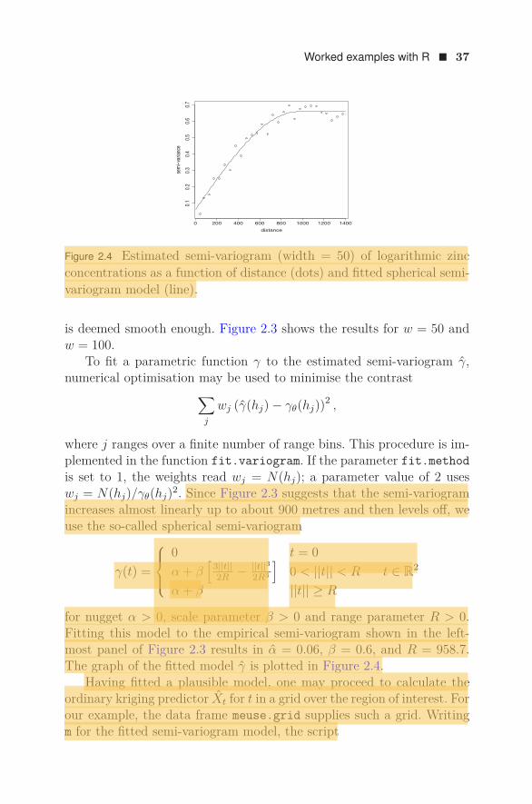
Figure 2.4 Estimated semi-variogram (width = 50) of logarithmic zincconcentrations as a function of distance (dots) and fitted spherical semi-variogram model (line).
is deemed smooth enough. Figure 2.3 shows the results for w = 50 andw = 100.
To fit a parametric function γ to the estimated semi-variogram γ,numerical optimisation may be used to minimise the contrast
∑
j
wj (γ(hj) − γθ(hj))2 ,
where j ranges over a finite number of range bins. This procedure is im-plemented in the function fit.variogram. If the parameter fit.methodis set to 1, the weights read wj = N(hj); a parameter value of 2 useswj = N(hj)/γθ(hj)2. Since Figure 2.3 suggests that the semi-variogramincreases almost linearly up to about 900 metres and then levels off, weuse the so-called spherical semi-variogram
γ(t) =
⎧⎪⎨
⎪⎩
0 t = 0α + β
[3||t||2R − ||t||3
2R3
]0 < ||t|| < R
α + β ||t|| ≥ R
t ∈ R2
for nugget α > 0, scale parameter β > 0 and range parameter R > 0.Fitting this model to the empirical semi-variogram shown in the left-most panel of Figure 2.3 results in α = 0.06, β = 0.6, and R = 958.7.The graph of the fitted model γ is plotted in Figure 2.4.
Having fitted a plausible model, one may proceed to calculate theordinary kriging predictor Xt for t in a grid over the region of interest. Forour example, the data frame meuse.grid supplies such a grid. Writingm for the fitted semi-variogram model, the script
38 ! Random field modelling and interpolation
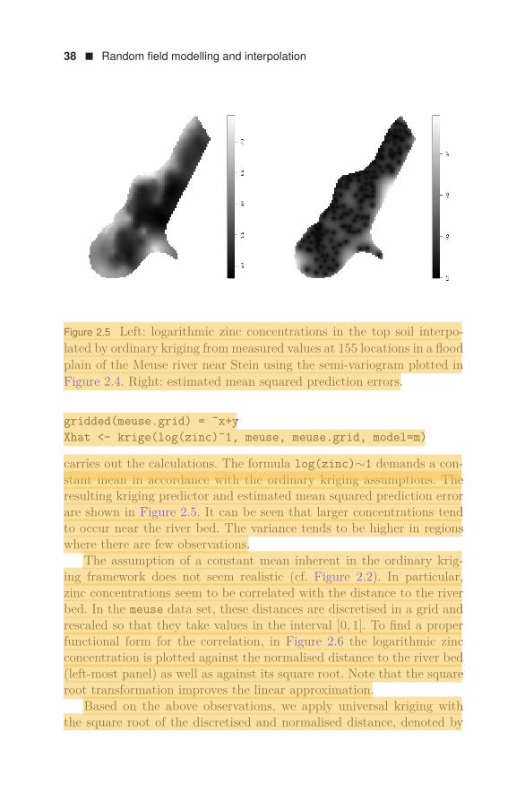
Figure 2.5 Left: logarithmic zinc concentrations in the top soil interpo-lated by ordinary kriging from measured values at 155 locations in a floodplain of the Meuse river near Stein using the semi-variogram plotted inFigure 2.4. Right: estimated mean squared prediction errors.
gridded(meuse.grid) = ˜x+yXhat <- krige(log(zinc)˜1, meuse, meuse.grid, model=m)
carries out the calculations. The formula log(zinc)∼1 demands a con-stant mean in accordance with the ordinary kriging assumptions. Theresulting kriging predictor and estimated mean squared prediction errorare shown in Figure 2.5. It can be seen that larger concentrations tendto occur near the river bed. The variance tends to be higher in regionswhere there are few observations.
The assumption of a constant mean inherent in the ordinary krig-ing framework does not seem realistic (cf. Figure 2.2). In particular,zinc concentrations seem to be correlated with the distance to the riverbed. In the meuse data set, these distances are discretised in a grid andrescaled so that they take values in the interval [0, 1]. To find a properfunctional form for the correlation, in Figure 2.6 the logarithmic zincconcentration is plotted against the normalised distance to the river bed(left-most panel) as well as against its square root. Note that the squareroot transformation improves the linear approximation.
Based on the above observations, we apply universal kriging withthe square root of the discretised and normalised distance, denoted by

Worked examples with R ! 39
0.0 0.2 0.4 0.6 0.8
5.0
5.5
6.0
6.5
7.0
7.5
Distance
Loga
rithm
ic zin
c con
cent
ratio
ns
0.0 0.2 0.4 0.6 0.8
5.0
5.5
6.0
6.5
7.0
7.5
Square root of distance
Loga
rithm
ic zin
c con
cent
ratio
ns
Figure 2.6 Logarithmic zinc concentrations in the top soil at 155 loca-tions in a flood plain of the Meuse river near Stein plotted against thenormalised distance to the river bed (left) and the square root of thenormalised distance to the river bed (right).
d(t), as a covariate. Thus, the log zinc concentrations follow the linearregression model
Xt = β0 + β1d(t) + Et,
where Et is a zero mean random field. The parameters β0 and β1 areassumed to be unknown.
To compute an empirical semi-variogram of the random field (Et)t,one must first estimate β = (β0, β1)′. The least squares estimator is
β = (M ′M)−1M ′Z,
where Z is the observation vector and M a 155 × 2 matrix whose firstcolumn contains entries that are all equal to 1. The i-th entry of thesecond column of M is the square root of the normalised distance fromthe grid cell of sampling location i to the river bed. Next, the semi-variogram of (Et)t can be estimated as before for the residuals Xt − β0 −β1d(t). The following script carries out these two tasks:
vdist <- variogram(log(zinc)˜sqrt(dist), meuse, cutoff=1300,width=50)
Figure 2.7 shows the residuals and the fitted spherical semi-variogram
mdist <- fit.variogram(vdist, vgm(0, "Sph", 100, 0),fit.method=1).

40 ! Random field modelling and interpolation
0 200 400 600 800 1000 1200
0.05
0.10
0.15
0.20
0.25
distance
sem
i−va
rianc
e
Figure 2.7 Estimated semi-variogram (width = 50) of residual logarithmiczinc concentrations as a function of distance (dots) and fitted sphericalsemi-variogram model (line). The residuals are obtained from a linearregression against the square root of the normalised distance to theriver bed.
Having fitted a plausible model incorporating the covariate informa-tion, we calculate the universal kriging predictor Xt for t in the grid sup-plied with the data. Writing mdist for the fitted semi-variogram model,the commandkrige(log(zinc)˜sqrt(dist), meuse, meuse.grid, model=mdist)carries out the calculations. Note that the formula now involves the co-variate dist in the the meuse data frame. The resulting kriging predictorand estimated mean squared prediction error are shown in Figure 2.8.Upon comparison with Figure 2.5, it can be seen that taking the distanceto the river into account leads to a smoother predictor and a smallerestimated mean squared prediction error.
To validate the final model, appropriate residuals are needed. Sincedata are available only at the measurement locations, we predict thelogarithmic zinc concentration in the top soil at a selected measurementlocation based on the concentrations at all other measurement locationsusing the model and subtract the result from the actual measurement.Repeating this procedure for all 155 locations yields the set of so-calledcross-validation residuals. The scriptkrige.cv(log(zinc)˜sqrt(dist), meuse, meuse.grid,model=mdist)carries out the computations. A graphical representation of the cross-validation procedure is shown in Figure 2.9. Since the mean value −0.003of the residuals is close to zero and there does not appear to be anyspatial pattern, we conclude that the model seems adequate.

Worked examples with R ! 41
4.5
5.0
5.5
6.0
6.5
7.0
0.10
0.12
0.14
0.16
0.18
0.20
Figure 2.8 Left: logarithmic zinc concentrations in the top soil interpo-lated by universal kriging from measured values at 155 locations in aflood plain of the Meuse river near Stein using the semi-variogram plot-ted in Figure 2.7. Right: estimated mean squared prediction errors.
For further details, we refer to the vignettes of RandomFields andgstat that are available on the CRAN websitehttps://cran.r-project.org.
−0.995−0.2160.0050.1841.544
Figure 2.9 Residuals of logarithmic zinc concentrations in the top soilinterpolated by cross-validated universal kriging from measured valuesat 155 locations in a flood plain of the Meuse river near Stein using thesemi-variogram plotted in Figure 2.7.

42 ! Random field modelling and interpolation
2.12 EXERCISES
1. Consider the random field (Xt)t∈Rd defined by
Xt = Z1t ∈ A
for a real-valued random variable Z and compact subset A of Rd.Express the finite dimensional distributions of X in terms of thecumulative distribution function of Z.
2. Fix n ∈ N and let fi : Rd → R, i = 1, . . . , n, be a set of functions.Let (Z1, . . . , Zn)′ be a random n-vector whose moments exist upto second order. Derive the covariance function of the random field
Xt =n∑
i=1Zifi(t), t ∈ Rd.
3. Let X = (Xt)t∈Rd be a Gaussian random field with mean func-tion m and covariance function ρ. Set Yt = X2
t . Show that themean function mY and covariance function ρY of the random field(Yt)t∈Rd are given by
mY (t) = m(t)2 + ρ(t, t)ρY (s, t) = 2ρ(s, t) ρ(s, t) + 2m(s)m(t)
for s, t ∈ Rd.Hint: You may use the Isserlis theorem stating that if (Z1, . . . , Z4)′
is a zero mean multivariate normally distributed random vector,then
E [Z1Z2Z3Z4] = E [Z1Z2]E [Z3Z4] + E [Z1Z3]E [Z2Z4]+ E [Z1Z4]E [Z2Z3] .
4. Show that if ρ1, ρ2 : Rd × Rd → R are non-negative definite, thenso are αρ1 + βρ2 (α, β ≥ 0) and ρ1ρ2.
5. Consider the function
ρ(t1, t2) = min(t1, t2), t1, t2 ∈ (0, ∞).
Show that ρ is non-negative definite.Hint: Use the Sylvester criterion.

Exercises ! 43
6. Compute the spectral measure of the 1-dimensional Ornstein–Uhlenbeck process with covariance function ρ(t) = exp(−β|t|)/(2β),t ∈ R, β > 0. Does this process admit a version with continuoussample paths?
7. Let θ(t) = (1 − |t|)+ for t ∈ R. Show that, for all ξ ∈ R,∫ ∞
−∞θ(t)e−iξtdt =
(sin(ξ/2)ξ/2
)2
by computing the Fourier transform of φ(t) = 1−1/2 ≤ t ≤ 1/2,t ∈ R, and relating φ to the triangle function θ.
8. Consider the function
ρ(θ) =∞∑
j=0σ2
j cos(jθ), θ ∈ [−π, π],
for σ2j = (α + βj2p)−1 and α, β > 0 (the generalised p-order model
of Hobolth, Pedersen and Jensen). For which p is ρ the covariancefunction of a Gaussian random field X? For which p does X admita continuous version?
9. Consider the spherical semi-variogram
γ(t) =
⎧⎪⎨
⎪⎩
0 t = 0α + β
[3|t|2 − |t|3
2
]0 < |t| < 1
α + β |t| ≥ 1t ∈ R
for α, β > 0. What are the nugget, sill and partial sill? Sketch thegraph.
10. Let X be a zero mean random field from which two observationsare available at t1 = t2. Moreover, suppose that
Cov(Xt1 , Xt2) = ρσ2
Cov(Xti , Xti) = σ2, i ∈ 1, 2,
for some known ρ ∈ (−1, 1) and σ2 > 0.
• Give the general expression for the best linear predictor (krig-ing estimator) at t0 ∈ t1, t2.

44 ! Random field modelling and interpolation
• Specialise to the case where ρ = 0, Cov(Xt0 , Xt1) = 0 andCov(Xt0 , Xt2) = 0.
• Specialise to the case where ρ = 0, Cov(Xt0 , Xt1) = 0 andCov(Xt0 , Xt2) = 0.
• What does your estimator look like when ρ = 0?• Calculate the mean squared prediction error for the above
special cases.
11. Consider the linear model
Xt = m(t)′β + Et, t ∈ Rd,
for some function m : Rd → Rp, β ∈ Rp and zero mean Gaussianrandom field (Et)t∈Rd .
• Propose a kriging estimator Xt0 based on observationsXt1 , . . . , Xtn when m and β are known. What assumptionsdo you make regarding (Et)t?
• If β were unknown, how would you proceed?
12. Let X be a random field from which two observations are availableat t1 = t2. Assume that
EXt1 = EXt2 = EXt0 = m
for some unknown m ∈ R and write
Cov(Xt1 , Xt2) = ρσ2
Cov(Xti , Xti) = σ2, i ∈ 1, 2,
for known ρ ∈ (−1, 1) and σ2 > 0.
• Give the general expression for the best linear predictor (krig-ing estimator) at t0 ∈ t1, t2.
• Specialise to the case where ρ = 0, Cov(Xt0 , Xt1) = 0 andCov(Xt0 , Xt2) = 0.
• Specialise to the case where ρ = 0, Cov(Xt0 , Xt1) = 0 andCov(Xt0 , Xt2) = 0.
• What does your estimator look like when ρ = 0?• Calculate the mean squared prediction error and compare to
that of simple kriging (cf. Exercise 10).

Exercises ! 45
13. Let Xt1 , . . . , Xtn be sampled from a zero mean random field(Xt)t∈Rd at n locations ti ∈ Rd, i = 1, . . . , n, and collected inthe n-vector Z. Write Σ = Cov(Z) and let K = (Ki)n
i=1 be then × 1 vector with entries Ki = ρ(ti, t0). If some eigenvalue of Σ iszero, show that K lies in the column space of Σ.
14. Consider the linear model
Xt = m(t)′β + Et, t ∈ Rd,
for some given function m : Rd → Rp, unknown parameter β ∈Rp and zero mean random field (Et)t∈Rd . Carry out the Euler–Lagrange optimisation to verify that the universal kriging predictorXt0 of Xt0 based on observation of Xt at t1, . . . , tn has the form(2.15).
15. The gstat package contains a data set coalash. Fit a semi-variogram model to these data and carry out an appropriate krig-ing analysis with particular attention to trends in the east-westdirection.

46 ! Random field modelling and interpolation
2.13 POINTERS TO THE LITERATURE
The mathematical theory of probability distributions defined as mea-sures, that is, satisfying a set of axioms, dates back to the famous 1933monograph by A.N. Kolmogoroff, which also contains the consistencytheorem [1, Section III.4]. The first textbook on stochastic processes waspublished by J.L. Doob in 1953 [2]. We refer specifically to Chapter II.3for a definition of Gaussian random fields and a proof of Proposition 2.1,and to Chapter II.8 for various concepts of stationarity. A current text-book is that by P. Billingsley [3]. In Chapter 7, he proves the consistencytheorem and applies it to the finite dimensional distributions of a ran-dom field. Part I of the book by Adler and Taylor [4] may be consultedfor a comprehensive overview of the theory of Gaussian random fields.
The Brownian motion, named in honour of the botanist R. Brownwho studied the movements of particles in a fluid, seems to have beenmodelled mathematically by T.N. Thiele [5] and, independently, by L.J.-B.A. Bachelier [6]. The Ornstein–Uhlenbeck covariance function was in-troduced in [7], whilst Mandelbrot and Van Ness [8] introduced the frac-tional Brownian surface. The latter is an example of the wider class ofintrinsic random functions [9].
Covariance functions are at the heart of geostatistics. For a surveyof the state of the art one may consult, for example, Chapter 2 by M.Schlather in [10] or M.L. Stein’s book [11]. In particular, Section 2.3in [11] collects elementary properties of covariance functions, includingProposition 2.2. The Whittle–Matern function is named after the pio-neers B. Matern (see [12], section 2.4) and P. Whittle [13]. Theorem 2.1is due to S. Bochner and can be found in Section 8 of his 1933 paper[14]. The proof given here is due to H. Cramer [15]. For the relationsbetween the spectral density and sample path properties, one may con-sult the early monograph by Cramer and Leadbetter [16], or the morerecent textbooks by R.J. Adler [17], Adler and Taylor [4] or Rogers andWilliams [18], for example. Proposition 2.3 is a spectral version of G.Matheron’s turning bands method (Section 4 in [9]). On a practical note,the R-package RandomFields may be used to generate realisations.
The origins of kriging are traced in a survey paper [19] by N. Cressiewho argues that L.S. Gandin [20] and G. Matheron [21, 22] indepen-dently discovered ordinary and simple kriging during the early 1960s.The Matheron estimator of the semi-variogram can be found in [21].Universal kriging is also due to G. Matheron [23]. There are many othervariations on kriging. For further details, including discussions on themerits and drawbacks, we refer the reader to the textbooks by Journel

References ! 47
and Huijbregts [24], Diggle and Ribeiro [25], Chiles and Delfiner [26] orto the relevant parts of Cressie [28], Bivand, Pebesma and Gomez–Rubio[29] and the Handbook of Spatial Statistics [27]. Implementations of krig-ing methods are available in the R-packages gstat, geoR, RandomFieldsand spatial. Finally, the Bayes estimator is well known in statisticaldecision theory; see for example Chapter 4 in Lehmann and Casella’stextbook in statistics [30].
REFERENCES
[1] A.N. Kolmogoroff (1933). Grundbegriffe der Wahrscheinlichkeitsrechnung. Re-printed in 1973 by Springer-Verlag.
[2] J.L. Doob (1953). Stochastic Processes. New York: John Wiley & Sons.
[3] P. Billingsley (2012). Probability and Measure (anniversary edition). Hoboken,New Jersey: John Wiley & Sons.
[4] R.J. Adler and J.E. Taylor (2007). Random Fields and Geometry. New York:Springer-Verlag.
[5] T.N. Thiele (1880). Sur la compensation de quelques erreurs quasi-systematiques par la methode des moindres carres. Reitzel.
[6] L.J.-B.A. Bachelier (1900). Theorie de la speculation. PhD thesis, Universityof Paris.
[7] G.E. Uhlenbeck and L.S. Ornstein (1930). On the theory of Brownian motion.Physical Review 36(5):823–841.
[8] B. Mandelbrot and J.W. van Ness (1968). Fractional Brownian motions, frac-tional noises and applications. SIAM Review 10(4):422–437.
[9] G. Matheron (1973). The intrinsic random functions and their applications.Advances in Applied Probability 5(3):439–468.
[10] M. Schlather (2012). Construction of covariance functions and unconditionalsimulation of random fields. Chapter 2 in: Advances and challenges inspace-time modelling of natural events. Springer Lecture Notes in Statis-tics 207.
[11] M.L. Stein (1999). Interpolation of Spatial Data. Some Theory for Kriging.New York: Springer-Verlag.
[12] B. Matern (1986). Spatial Variation (2nd edition). Berlin: Springer-Verlag.
[13] P. Whittle (1962). Topographic correlation, power-law covariance functions,and diffusion. Biometrika 49(3/4):305–314.

48 ! Random field modelling and interpolation
[14] S. Bochner (1933). Monotone Funktionen, Stieltjessche Integrale und har-monische Analyse. Mathematische Annalen 108(1):378–410.
[15] H. Cramer (1939). On the representation of a function by certain Fourier inte-grals. Transactions of the American Mathematical Society 46(2):191–201.
[16] H. Cramer and M.R. Leadbetter (1967). Stationary and Related Stochas-tic Processes. Sample Function Properties and Their Applications. NewYork: John Wiley & Sons.
[17] R.J. Adler (1981). The Geometry of Random Fields. New York: John Wiley &Sons.
[18] L.C.G. Rogers and D. Williams (1994). Diffusions, Markov Processes and Mar-tingales. Volume 1: Foundations (2nd edition). Chichester: John Wiley &Sons.
[19] N. Cressie (1990). The origins of kriging. Mathematical Geology 22(3):239–252.
[20] L.S. Gandin (1963). Objective Analysis of Meteorological Fields. Translated byIsrael Program for Scientific Translations, 1965.
[21] G. Matheron (1962). Traite de geostatistique appliquee, Volume I. Mem-oires du Bureau de Recherches Geologiques et Minieres no 14. EditionsTechnip.
[22] G. Matheron (1963). Traite de geostatistique appliquee, Volume II. Mem-oires du Bureau de Recherches Geologiques et Minieres no 24. EditionsTechnip.
[23] G. Matheron (1969). Le krigeage universel. Cahiers du Centre de MorphologieMathematique no 1.
[24] A.G. Journel and C.J. Huijbregts (1978). Mining Geostatistics. London: Aca-demic Press.
[25] P.J. Diggle and P.J. Ribeiro Jr (2008). Model-Based Geostatistics. New York:Springer-Verlag.
[26] J.-P. Chiles and P. Delfiner (2012). Geostatistics: Modeling Spatial Uncertainty(2nd edition). Hoboken, New Jersey: John Wiley & Sons.
[27] A.E. Gelfand, P.J. Diggle, M. Fuentes and P. Guttorp, editors (2010). Hand-book of Spatial Statistics. Boca Raton, Florida: Chapman & Hall/CRC.
[28] N.A.C. Cressie (2015). Statistics for Spatial Data (revised edition). New York:John Wiley & Sons.
[29] R.S. Bivand, E. Pebesma and V. Gomez–Rubio (2013). Applied Spatial DataAnalysis with R (2nd edition). New York: Springer-Verlag.
[30] E.L. Lehmann and G. Casella (1998). Theory of Point Estimation (2nd edi-tion). New York: Springer-Verlag.

C H A P T E R 3
Models and inferencefor areal unit data
3.1 DISCRETE RANDOM FIELDS
In this chapter, we will study random field models with a discrete indexset. Such models are useful when observations are collected over arealunits such as pixels, census districts or tomographic bins. In contrast tothe previous chapter, the aims are noise removal and smoothing ratherthan interpolation.
Mathematically speaking, the index set T of the random field X isfinite. In statistical physics, T may be a collection of atoms and gen-uinely finite; more often, Xi represents an integral or average of thephenomenon of interest over some region represented by i ∈ T . Often,there is a natural adjacency relation or neighbourhood structure.
Definition 3.1 Let T = ∅ be a finite collection of ‘sites’. A random fieldX on T with values in L is a random vector (Xi)i∈T having L–valuedcomponents. If L is finite or countably infinite, the distribution of X isspecified by the probability mass function
πX(x) = P(X = x) = P(Xi = xi, i ∈ T ), x ∈ LT .
Otherwise, we assume that L ⊆ R and that X is absolutely continuouswith a joint probability density πX .
An example with a finite label set L is the following.
Example 3.1 Presence/absence data record 1 if a phenomenon of in-terest is observed in the region represented by i ∈ T and 0 otherwise.
49

50 ! Models and inference for areal unit data
Hence L = 0, 1. Write i ∼ j if the regions corresponding to i andj are adjacent. Then the Ising model is defined by the probability massfunction
πX(x) ∝ exp
⎡
⎣α∑
i∈T
xi + β∑
i,j:i∼j
xixj
⎤
⎦ , x ∈ LT ,
for constants α, β ∈ R. The parameter α influences the prevalence. In-deed, if β = 0, in each region, the phenomenon of interest is observedwith probability eα/(1 + eα) independently of other regions. For β > 0,presence in a given region encourages presence in neighbouring regions,whereas for β < 0 such presence is discouraged. As an aside, the Isingmodel is also used in statistical physics to describe magnetisation, usuallywith the label set L = −1, +1.
In the next example, the label set L is equal to R.Example 3.2 Conditional autoregression (CAR) models can be definedby requiring the random field X to be multivariate normally distributedwith mean zero and covariance matrix (I − B)−1K, where K = diag(κi)is a diagonal matrix with κi > 0, I − B is non-singular and (I − B)−1Kis symmetric and positive definite. The scale is fixed by assuming thatthe diagonal elements of B are zero.
Usually the matrix B is sparse; for instance B = φN could be pro-portional to the neighbourhood matrix N defined by Nij = 1i ∼ j forsome symmetric neighbourhood relation ∼ on T . To ensure that bii = 0,the relation should be non-reflexive, that is i ∼ i for all i ∈ T . In theliterature, N is also known as the adjacency or contiguity matrix.
To verify that a matrix is positive definite, the Gershgorin disc the-orem is useful. It states that, for a symmetric matrix A, the conditionsaii > 0 and aii >
∑j =i |aij | imply that A is positive definite. Applied to
I − φN , a sufficient condition is that for each site, |φ| is smaller thanthe reciprocal of the number of neighbours of that site.
Write XA for the restriction of X to sites in the set A ⊂ T . In thecase of finite L, conditional probabilities of the type
πA(xA | xT \A) = P(XA = xA | XT \A = xT \A)
are of interest. In the absolutely continuous case, πA is defined as theconditional probability density, provided it exists.
An important special case is A = i, yielding the following defini-tion. To improve readability, write T \ i for the set T \ i.

Discrete random fields ! 51
Definition 3.2 Let T = ∅ be a finite collection of sites. The local char-acteristics of a random field X on T with values in L are
πi(xi | xT \i), i ∈ T, x ∈ LT ,
whenever well-defined.
Example 3.3 For the Ising model introduced in Example 3.1,
log[
πi(1 | xT \i)πi(0 | xT \i)
]
= α + β∑
j∼i
xj .
Therefore, the Ising model is also known as (first-order) auto-logisticregression and
πi(1 | xT \i) =exp
[α + β
∑j∼i xj
]
1 + exp[α + β
∑j∼i xj
] .
It is interesting to note that πi(· | xT \i) depends only on values xj forregions indexed by neighbours of i.
Example 3.4 For the CAR model of Example 3.2, the local character-istics are Gaussian distributions with
E(Xi | Xj , j = i) = ∑
j =i bijXj
Var(Xi | Xj , j = i) = κi(3.1)
These expressions justify the name ‘conditional autoregression’. In par-ticular, if bij = φNij, (3.1) involves only the neighbours of site i. Theresult can be proved by basic but tedious matrix algebra. We will give amore elegant proof below.
For strictly positive distributions, the local characteristics determinethe entire distribution. The proof relies on the following theorem.
Theorem 3.1 (Besag’s factorisation theorem – Brook’s lemma)Let X be an L-valued random field on T = 1, . . . , N, N ∈ N, suchthat πX(x) > 0 for all x ∈ LT . Then, for all x, y ∈ LT ,
πX(x)πX(y) =
N∏
i=1
πi(xi | x1, . . . , xi−1, yi+1, . . . , yN )πi(yi | x1, . . . , xi−1, yi+1, . . . , yN ) . (3.2)

52 ! Models and inference for areal unit data
Proof: Due to the positivity assumption, one never divides by zero.Now,
πX(x) = πN (xN | x1, . . . , xN−1)πN (yN | x1, . . . , xN−1) πX(x1, . . . , xN−1, yN ).
Similarly, πX(x1, . . . , xN−1, yN ) factorises as
πN−1(xN−1 | x1, . . . , xN−2, yN )πN−1(yN−1 | x1, . . . , xN−2, yN ) πX(x1, . . . , xN−2, yN−1, yN ).
The claim is seen to hold by iterating the above argument. "
On a cautionary note, the converse does not hold in the sense that itis not always possible to construct a joint distribution from arbitrarilychosen πi(·|·).
Corollary 3.1 Let X be an L-valued random field on a finite collectionT = ∅ of sites such that πX(x) > 0 for all x ∈ LT . Then the localcharacteristics determine the whole distribution, that is, if Y is a randomfield having the same local characteristics as X, necessarily πY ≡ πX .
Proof: Choose any element a ∈ L. Then, by Besag’s factorisation theo-rem, πX(x)/ πX(a, . . . , a) is determined by the local characteristics. Thedistribution is obtained by normalisation. "
3.2 GAUSSIAN AUTOREGRESSION MODELS
Recall the following definition (cf. Example 3.2).
Definition 3.3 Let K = diag(κi) be a diagonal N ×N matrix with κi >0 and B an N × N matrix whose diagonal elements bii are zero. Then,provided I −B is invertible and (I −B)−1K is positive definite, a randomfield X that is normally distributed with mean zero and covariance matrix(I −B)−1K is said to follow a conditional autoregression (CAR) model.
The name is justified by the fact that if one specifies local character-istics as in (3.1), then relative to (yi)i=1,...,N = 0,
πi(xi|x1, . . . , xi−1, yi+1, . . . , yN )πi(yi|x1, . . . , xi−1, yi+1, . . . , yN ) =
exp[− 1
2κi(xi −
∑j<i bijxj)2
]
exp[− 1
2κi(∑j<i bijxj)2
]
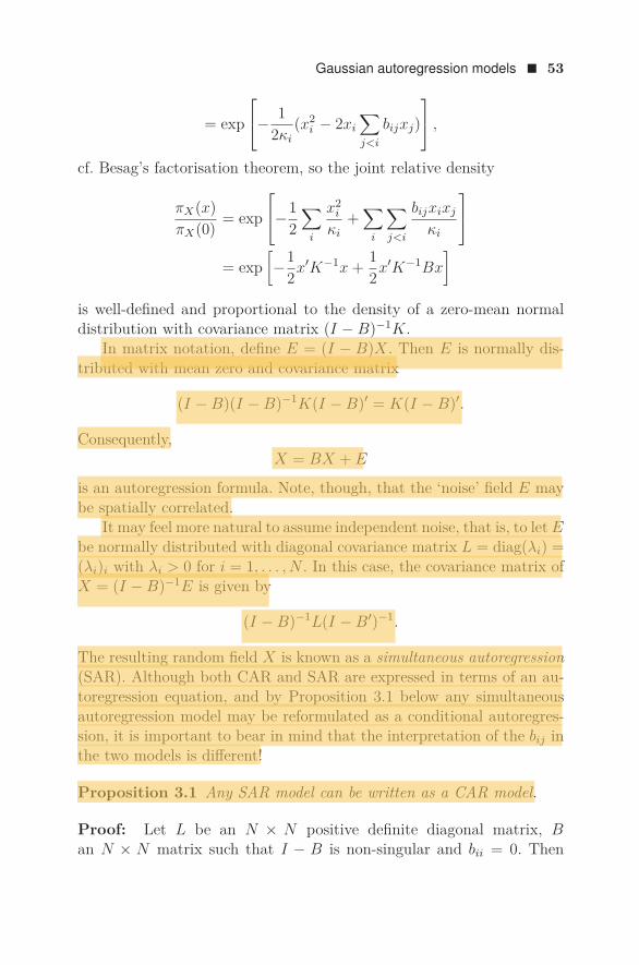
Gaussian autoregression models ! 53
= exp
⎡
⎣− 12κi
(x2i − 2xi
∑
j<i
bijxj)
⎤
⎦ ,
cf. Besag’s factorisation theorem, so the joint relative density
πX(x)πX(0) = exp
⎡
⎣−12
∑
i
x2i
κi+
∑
i
∑
j<i
bijxixj
κi
⎤
⎦
= exp[−1
2x′K−1x + 12x′K−1Bx
]
is well-defined and proportional to the density of a zero-mean normaldistribution with covariance matrix (I − B)−1K.
In matrix notation, define E = (I − B)X. Then E is normally dis-tributed with mean zero and covariance matrix
(I − B)(I − B)−1K(I − B)′ = K(I − B)′.
Consequently,X = BX + E
is an autoregression formula. Note, though, that the ‘noise’ field E maybe spatially correlated.
It may feel more natural to assume independent noise, that is, to let Ebe normally distributed with diagonal covariance matrix L = diag(λi) =(λi)i with λi > 0 for i = 1, . . . , N . In this case, the covariance matrix ofX = (I − B)−1E is given by
(I − B)−1L(I − B′)−1.
The resulting random field X is known as a simultaneous autoregression(SAR). Although both CAR and SAR are expressed in terms of an au-toregression equation, and by Proposition 3.1 below any simultaneousautoregression model may be reformulated as a conditional autoregres-sion, it is important to bear in mind that the interpretation of the bij inthe two models is different!
Proposition 3.1 Any SAR model can be written as a CAR model.
Proof: Let L be an N × N positive definite diagonal matrix, Ban N × N matrix such that I − B is non-singular and bii = 0. Then

54 ! Models and inference for areal unit data
(I − B)−1L(I − B′)−1 is well-defined, symmetric and positive definite.One needs to solve
(I − B)−1L(I − B′)−1 = (I − C)−1K
for C and K = diag(κi), or, equivalently,
(I − B′)L−1(I − B) = K−1(I − C).
Setting cii = 0, it remains to solve for the scale factors κi. Indeed, writingλi for the i-th element on the diagonal of L, for all i ∈ 1, . . . , N,
1λi
+N∑
j=1
b2ji
λj= 1
κi,
and therefore κi > 0. "
There is a price to pay for the uncorrelated noise in SAR models. Tosee this, note that for a CAR model
Cov(E, X) = E(EX ′) = Cov((I − B)X, X) = (I − B)(I − B)−1K = K.
Consequently Xi and Ej are independent for i = j. For SAR models,such a remark does not necessarily hold. Indeed,
Cov(X, E) = Cov((I − B)−1E, E) = (I − B)−1L
may be non-diagonal.To conclude this section, it is worth noticing that one would often
like to define⎧⎨
⎩E(Xi | Xj , j = i) =
∑j =i
NijXj∑j =i
Nij
Var(Xi | Xj , j = i) = κi
(3.3)
for Nij as in Example 3.2. In other words, bij = Nij/∑
k =i Nik. However,for such models I − B may no longer be invertible due to the row sumsbeing zero. Nevertheless, intrinsic autoregression models ‘defined’ by(3.3) are often used as ‘prior distribution’ in a hierarchical Bayesianmodel.

Gibbs states ! 55
3.3 GIBBS STATES
The log probability mass function of the Ising model can be interpretedas a sum of contributions from single sites and pairs of sites. Breakingup a high-dimensional joint probability mass function in lower dimen-sional components in this way is often useful, both from a computationalpoint of view and conceptually, for example in defining new models orin formalising the notion of interaction.
Definition 3.4 Let T = ∅ be a finite collection of sites, L a subset of R.An interaction potential is a collection VA : A ⊆ T of functions VA :LT → R such that V∅(·) ≡ 0 and VA(x) depends only on the restrictionxA of x ∈ LT to sites in A.
The interaction potential V is said to be normalised with respect toa ∈ L if the property that xi = a for some i ∈ A implies that VA(x) = 0.
A random field whose distribution is defined in terms of interactionpotentials is known as a Gibbs state.
Definition 3.5 Let X be an L-valued random field on a finite collectionT = ∅ of sites and V an interaction potential. Then X is a Gibbs statewith interaction potentials V = VA : A ⊆ T, VA : LT → R, if
πX(x) = 1Z
exp
⎡
⎣∑
A⊆T
VA(xA)
⎤
⎦ , x ∈ LT . (3.4)
The constant Z in (3.4) is called the partition function and is usuallyintractable, both analytically and numerically.
Example 3.5 The auto-logistic regression model introduced in Exam-ple 3.1 is a Gibbs state with interaction potentials
Vi(x) = αxi
Vi,j(x) =
βxixj if i ∼ j0 else
and VA(x) = 0 for sets A of cardinality larger than two.

56 ! Models and inference for areal unit data
Example 3.6 Let X be multivariate normally distributed with meanvector µ and positive definite covariance matrix Σ and write Q = Σ−1
for the precision matrix. Then, since
πX(x) ∝ exp
⎡
⎣−12
∑
i
∑
j
(xi − µi)Qij(xj − µj)
⎤
⎦ ,
X is a Gibbs state with interaction potentialsVi(x) = −Qii(xi − µi)2/2
Vi,j(x) = −Qij(xi − µi)(xj − µj) (3.5)upon recalling that Q, being a precision matrix, is symmetric. For setsA of cardinality larger than two, VA(x) = 0.
In fact, any random field X such that πX(x) > 0 for all x is a Gibbsstate.
Theorem 3.2 Let X be an L-valued random field on a finite collectionT = ∅ of sites such that πX(x) > 0 for all x ∈ LT . Then X is a Gibbsstate with respect to the canonical potential
VA(x) =∑
B⊆A
(−1)|A\B| log πX(xB), x ∈ LT ,
where xBi = xi for i ∈ B and a prefixed value a ∈ L otherwise. This
is the unique normalised potential with respect to a. Moreover, for anyelement i ∈ A,
VA(x) =∑
B⊆A
(−1)|A\B| log πi(xBi | xB
T \i), x ∈ LT . (3.6)
The proof relies on the following combinatorial identity.
Theorem 3.3 (Mobius inversion formula) If T is a finite set andf, g : P (T ) → R are two functions defined on the power set P (T ) of T ,then
f(A) =∑
B⊆A
g(B) for all A ⊆ T (3.7)
if and only ifg(A) =
∑
B⊆A
(−1)|A\B|f(B) for all A ⊆ T. (3.8)
In particular, there is only one way to represent a given function f inthe form (3.7).

Gibbs states ! 57
Proof: First suppose g is fixed and define f(A) = ∑B⊆A g(B) for
A ⊆ T . Then
∑
B⊆A
(−1)|A\B|f(B) =∑
B⊆A
(−1)|A\B|
⎡
⎣∑
C⊆B
g(C)
⎤
⎦
=∑
B⊆A
⎡
⎣∑
C⊆B
(−1)|A\C|(−1)−|B\C|g(C)
⎤
⎦
=∑
C⊆A
⎡
⎣∑
B:C⊆B⊆A
(−1)|B\C|
⎤
⎦ (−1)|A\C|g(C) = g(A).
For the last equality, note that the inner sum|A\C|∑
k=0
(|A \ C|
k
)
(−1)k
equals 0, unless A = C.Conversely, if f is fixed and g(A) = ∑
B⊆A(−1)|A\B|f(B), then
∑
B⊆A
g(B) =∑
B⊆A
⎡
⎣∑
C⊆B
(−1)|B\C|f(C)
⎤
⎦
=∑
C⊆A
⎡
⎣∑
B:C⊆B⊆A
(−1)|B\C|
⎤
⎦ f(C) = f(A)
by similar arguments. "
We are now ready to give the proof of Theorem 3.2.Proof: Fix x ∈ LT . Since πX(x) > 0 we can set, for A ⊆ T , fx(A) =log πX(xA). Define the interaction potential VA : LT → R by
VA(x) =∑
B⊆A
(−1)|A\B|fx(B), x ∈ LT .
By the Mobius inversion formula
fx(T ) =∑
A⊆T
VA(x)
or, equivalently,
πX(x) = exp[fx(T )] = exp
⎡
⎣∑
A⊆T
VA(x)
⎤
⎦ .

58 ! Models and inference for areal unit data
Now letting x vary, this identity shows that πX is a Gibbs state withinteraction potential VA : A ⊆ T upon incorporating V∅ into thepartition function if necessary.
To prove that the interaction potential is normalised, choose anyi ∈ A. Then
VA(x) =∑
i∈B⊆A
(−1)|A\B| log πX(xB) +∑
i∈B⊆A
(−1)|A\B| log πX(xB)
=∑
B⊆A\i(−1)|A\B| log πX(xB) −
∑
B⊆A\i(−1)|A\B| log πX(xB∪i)
=∑
B⊆A\i(−1)|A\B|
[log πX(xB) − log πX(xB∪i)
].
If xi = a, then xB = xB∪i for all B ⊆ A \ i and therefore VA(x) = 0.We conclude that the interaction potential is normalised with respectto a. Moreover xB
T \i = xB∪iT \i for all B ⊆ A \ i. Therefore
πX(xB)πX(xB∪i) =
πi(xBi | xB
T \i)πi(xB∪i
i | xB∪iT \i )
and the expression in terms of the local characteristics follows.Next suppose πX is a Gibbs state with respect to normalised poten-
tials UA. We will show that UA ≡ VA. Write aT for the realisation withonly a–labels and fix x ∈ LT . Define the set function hx(A) by
hx(A) = log πX(xA)πX(aT ) =
∑
B⊆A
[UB(x) − UB(aT )] =∑
B⊆A
UB(x).
The last equation uses the assumption that the interaction potential Uis normalised. By Theorem 3.3, for all A = ∅,
UA(x) =∑
B⊆A
(−1)|A\B|hx(B) = VA(x)−log πX(aT )∑
B⊆A
(−1)|A\B| = VA(x).
Finally, since VA(x) = UA(x) = 0 by assumption when A = ∅, the proofis complete. "
Example 3.7 Consider a multivariate normally distributed randomfield X with precision matrix Q as in Example 3.6. If the mean vec-tor is constant, that is, µi ≡ µ0 for all i ∈ T , the natural potential (3.5)

Markov random fields ! 59
is clearly normalised with respect to µ0. For inhomogeneous models, onemay normalise with respect to zero. Then for x ∈ RT , using the notationof Theorem 3.2, by definition V∅(x) = 0,
Vi(x) = log πX(xi) − log πX(0) = −12x2
i Qii + xi
∑
j∈T
µjQij
and, for i = j,
Vi,j(x) = log πX(xi,j) − log πX(xi) − log πX(xj) + log πX(0)= −xixjQij .
Note that Vi,j is equal to zero when Qij is.
3.4 MARKOV RANDOM FIELDS
Suppose that the set of sites T is equipped with a symmetric relation ∼.If the interaction potentials VA(x) vanish except when A is a singletonor consists of a pair i, j of ∼-related sites, as in Example 3.5, thelocal characteristics πi(· | xT \i) depend only on the values xj at sitesj ∈ T \ i that are ∼-neighbours of i. More generally, one may formulatethe following definition.
Definition 3.6 Let ∼ be a symmetric relation on the finite set T =∅ and define the boundary of A ⊆ T by ∂A = s ∈ T \ A : s ∼ tfor some t ∈ A. A random field X on T is a Markov random field withrespect to ∼ if
πi(xi | xT \i) = πX(Xi = xi | X∂i = x∂i)
whenever πX(xT \i) > 0, where πX denotes the probability mass functionof X if X takes values in a finite or countable set L and a probabilitydensity if X is absolutely continuous on L ⊆ R.
In other words, for a Markov random field, the conditional distribu-tion of the label at some site i given those at all other sites depends onlyon the labels at neighbours of site i.
Definition 3.7 Let T = ∅ be a finite collection of sites. Let ∼ be asymmetric relation on T . A clique, with respect to ∼, is a subset C ⊂ Tfor which s ∼ t for all s = t ∈ C. The family of all cliques is denotedby C.

60 ! Models and inference for areal unit data
Note that, by default, singletons and the empty set are cliques.
Theorem 3.4 (Hammersley–Clifford) Let X be an L-valued ran-dom field on a finite collection T = ∅ of sites such that πX(x) > 0 forall x ∈ LT . Let ∼ be a symmetric relation on T . Then X is a Markovrandom field with respect to ∼ if and only if
πX(x) =∏
C∈CϕC(xC) (3.9)
for some interaction functions ϕC : LC → R+ defined on cliques C ∈ C.
In other words, the distribution of any Markov random field suchthat πX is positive can be expressed in terms of interactions betweenneighbours. Moreover, by the positivity condition, equation (3.9) can berewritten as
πX(x) = exp[
∑
C∈Clog ϕC(xC)
]
,
so X is a Gibbs state with non-zero interaction potentials log ϕC
restricted to cliques.
Proof: First we show that any distribution of the form (3.9) has theMarkov property. Suppose that L is countable and write T a
i x for theconfiguration in which xi is replaced by a. Then
πi(xi | xT \i) =∏
C∋i ϕC(xC)∑
a∈L [∏C∋i ϕC(T ai xC)]
and the right-hand side depends only on xi and x∂i. In the absolutelycontinuous case, replace the sum over L by an integral.
Conversely suppose that X is a Markov random field with πX > 0.By Theorem 3.2, X is a Gibbs state with canonical potential (3.6). Weclaim that VA(x) = 0 for all A ∈ C. Indeed, if A ⊆ T is not a clique,there are two distinct sites s, t ∈ A with s ∼ t. Then
VA(x) =∑
B⊆A
(−1)|A\B| log πs(xBs | xB
T \s),
which can be written as the sum of four terms:∑
B⊆A\s,t(−1)|A\B| log πs(xB
s | xBT \s)
+∑
B⊆A\s,t(−1)|A\(B∪s)| log πs(xB∪s
s | xB∪sT \s )

Markov random fields ! 61
+∑
B⊆A\s,t(−1)|A\(B∪t)| log πs(xB∪t
s | xB∪tT \s )
+∑
B⊆A\s,t(−1)|A\(B∪s,t)| log πs(xB∪s,t
s | xB∪s,tT \s ).
Rearranging terms, it follows that
VA(x) =∑
B⊆A\s,t(−1)|A\B| log
⎡
⎣πs(xB
s | xBT \s)πs(xB∪s,t
s | xB∪s,tT \s )
πs(xB∪ts | xB∪t
T \s )πs(xB∪ss | xB∪s
T \s )
⎤
⎦ .
Since s ∼ t, πs(xBs | xB
T \s) = πs(xB∪ts | xB∪t
T \s ) and πs(xB∪ss |
xB∪sT \s ) = πs(xB∪s,t
s | xB∪s,tT \s ) and hence VA(x) = 0. Thus the only
nonzero interaction potentials are for cliques and (3.9) holds. "
Example 3.8 For the auto-logistic regression model, the interactionfunctions are
ϕ∅ = 1/Z
ϕi(xi) = exp(αxi)
ϕi,j(xi,j) =
exp(βxixj) if i ∼ j1 else
All higher order interaction functions take the constant value 1.
The positivity condition is needed, as demonstrated by the followingexample.
Example 3.9 Let T be a 2 × 2 grid equipped with the relation ∼ underwhich horizontally or vertically adjacent sites are related. Order the sitesin row major order. Set L = 0, 1 and let X be an L-valued randomfield on T such that
πX(0, 0, 0, 0) = πX(0, 1, 0, 0) = πX(0, 1, 0, 1) = πX(0, 1, 1, 1)
= πX(1, 1, 1, 1) = πX(1, 0, 1, 1) = πX(1, 0, 1, 0) = πX(1, 0, 0, 0) = 1/8and zero otherwise. Then X is Markov, since, for example,
π1(1 | 0, 1, 0) = 1 = π1(1 | 0, 1, 1) = P(X1 = 1 | X2 = 0, X3 = 1)

62 ! Models and inference for areal unit data
orπ1(1 | 0, 0, 0) = 1/2 = P(X1 = 1 | X2 = 0, X3 = 0).
It is left to the reader to verify the remaining cases. The probability massfunction πX cannot be factorised over cliques. To see this, suppose thatit is. Then, as πX(0, 1, 1, 0) = 0, the product
ϕ∅ϕ1(0)ϕ2(1)ϕ3(1)ϕ4(0)ϕ1,2(0, 1)ϕ1,3(0, 1)ϕ2,4(1, 0)ϕ3,4(1, 0)
must also be zero. However, all terms are positive, occurring as theydo in the factorisation of some x ∈ LT for which πX(x) > 0, and onearrives at a contradiction.
Corollary 3.2 Let X be an L-valued random field on a finite collectionT = ∅ of sites such that πX(x) > 0 for all x ∈ LT . Then the spatialMarkov property
π(XA = xA | XT \A = xT \A) = π(XA = xA | X∂A = x∂A)
holds for all nonempty sets A ⊆ T .
Proof: Write T yAx for the configuration in which xA is replaced by y
(xA, y ∈ LA) on the set A ⊆ T . By the Hammersley-Clifford theorem,
π(XA = xA | XT \A = xT \A) =∏
A∩C =∅ ϕC(xC)∑
y∈LA
∏A∩C =∅ ϕC((T y
Ax)C)
depends only on x∂A. "
3.5 INFERENCE FOR AREAL UNIT MODELS
Suppose that some spatial variable of interest is observed in a finite setof areal units and that the dependence of the variable on covariates isexpressed through a design matrix X and parameter vector β ∈ Rp.
In an autoregression context, for example in a SAR model, this ideais formalised as follows. Write Y = (Y1, . . . , Yn)′ for the random field. IfEY = Xβ for the n × p design matrix X and β ∈ Rp, the simultaneousauto-regression equation for Y − Xβ reads
Y = BY + (I − B)Xβ + E

Inference for areal unit models ! 63
where B is a known n × n matrix with bii = 0, for example propor-tional to the neighbourhood matrix, and E is n-variate Gaussian noise.For simplicity, assume that Cov(E) = σ2I. As before, we assume that(I − B) is non-singular, in which case the covariance matrix of Y isσ2(I − B)−1(I − B′)−1.
Inference regarding the parameters β and σ2 can be based on the loglikelihood L(β, σ2; Y ), which reads
− 12σ2 (Y −Xβ)′(I−B)′(I−B)(Y −Xβ)+log det(σ2(I−B)−1(I−B′)−1)−1/2.
Since the determinant is equal to σ2n det(I − B)−2, upon deletion ofterms that do not depend on the parameters σ2 and β, the log likelihoodreduces to
L(β, σ2; Y ) = − 12σ2 (Y − Xβ)′(I − B)′(I − B)(Y − Xβ) − n log σ.
Therefore, the score equations are
0 = −n
σ+ 1
σ3 (Y − Xβ)′(I − B)′(I − B)(Y − Xβ);
0 = X ′(I − B)′(I − B)(Y − Xβ),
which can be solved explicitly. Indeed
σ2 = 1n
(Y − Xβ)′(I − B)′(I − B)(Y − Xβ)
is the usual population variance and
β = (X ′(I − B)′(I − B)X)−1X ′(I − B)′(I − B)Y,
provided X ′(I − B)′(I − B)X is non-singular. Since Y is Gaussian, so isβ. Moreover,
Eβ = β;Cov(β) = σ2(X ′(I − B)′(I − B)X)−1.
As for nσ2, it is of quadratic form U ′U = ∑nj=1 U2
j . The random vectorU = (I − B)(Y − Xβ) is normally distributed with mean vector zero. Ingeneral, however, the Uj are not independent.
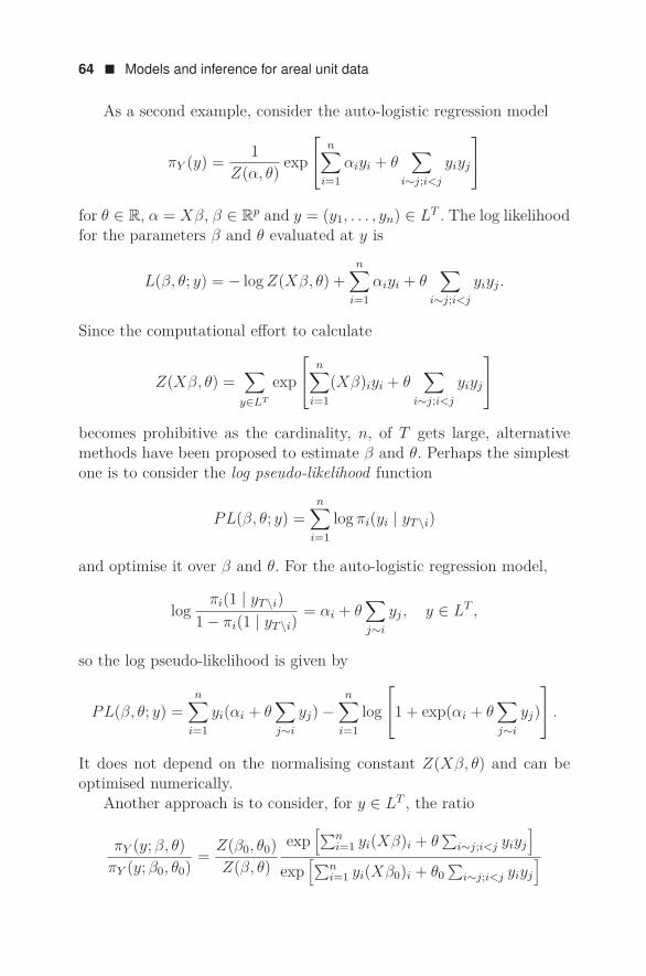
64 ! Models and inference for areal unit data
As a second example, consider the auto-logistic regression model
πY (y) = 1Z(α, θ) exp
⎡
⎣n∑
i=1αiyi + θ
∑
i∼j;i<j
yiyj
⎤
⎦
for θ ∈ R, α = Xβ, β ∈ Rp and y = (y1, . . . , yn) ∈ LT . The log likelihoodfor the parameters β and θ evaluated at y is
L(β, θ; y) = − log Z(Xβ, θ) +n∑
i=1αiyi + θ
∑
i∼j;i<j
yiyj .
Since the computational effort to calculate
Z(Xβ, θ) =∑
y∈LT
exp
⎡
⎣n∑
i=1(Xβ)iyi + θ
∑
i∼j;i<j
yiyj
⎤
⎦
becomes prohibitive as the cardinality, n, of T gets large, alternativemethods have been proposed to estimate β and θ. Perhaps the simplestone is to consider the log pseudo-likelihood function
PL(β, θ; y) =n∑
i=1log πi(yi | yT \i)
and optimise it over β and θ. For the auto-logistic regression model,
log πi(1 | yT \i)1 − πi(1 | yT \i)
= αi + θ∑
j∼i
yj , y ∈ LT ,
so the log pseudo-likelihood is given by
PL(β, θ; y) =n∑
i=1yi(αi + θ
∑
j∼i
yj) −n∑
i=1log
⎡
⎣1 + exp(αi + θ∑
j∼i
yj)
⎤
⎦ .
It does not depend on the normalising constant Z(Xβ, θ) and can beoptimised numerically.
Another approach is to consider, for y ∈ LT , the ratio
πY (y; β, θ)πY (y; β0, θ0) = Z(β0, θ0)
Z(β, θ)exp
[∑ni=1 yi(Xβ)i + θ
∑i∼j;i<j yiyj
]
exp[∑n
i=1 yi(Xβ0)i + θ0∑
i∼j;i<j yiyj
]

Inference for areal unit models ! 65
with respect to some fixed reference parameter values β0 and θ0. A crucialobservation is that the ratio of partition functions can be written as
Z(β, θ)Z(β0, θ0) = Eβ0,θ0
⎡
⎣exp
[∑ni=1 Yi(Xβ)i + θ
∑i∼j;i<j YiYj
]
exp[∑n
i=1 Yi(Xβ0)i + θ0∑
i∼j;i<j YiYj
]
⎤
⎦ ,
where Eβ0,θ0 denotes the expectation of the random field Y having prob-ability distribution πY with parameters β0 and θ0. Therefore, the ratioof normalising constants can be approximated by an empirical averageover a sample from the auto-logistic regression model under the referenceparameters β0 and θ0. We shall discuss in Section 3.6 how to generatesuch a sample.
The auto-logistic regression model is an exponential family. For suchmodels, under mild conditions, maximum likelihood estimators exist.
Theorem 3.5 Let Y be an L-valued random field on a finite collectionT = ∅ of sites whose probability mass function or joint probability densityis of the form
πY (y) = 1Z(θ) exp [θ′S(y)] , y ∈ LT ,
for some function S : LT → Rp, the sufficient statistic, and parameterθ ∈ Rp. Provided the moments of the random variable S(Y ) exist upto second order, the log likelihood function L(θ; y) is twice differentiablewith gradient
S(y) − EθS(Y )and non-positive definite Hessian −CovθS(Y ).
Proof: For the realisation y ∈ LT the log likelihood function
L(θ; y) = − log Z(θ) + θ′S(y)
is differentiable with gradient
∇L(θ; y) = S(y) − 1Z(θ)∇Z(θ).
Since Z(θ) = ∑y∈LT exp [θ′S(y)] , its gradient can be written as
∇Z(θ) =∑
y∈LT
S(y) exp [θ′S(y)] ,
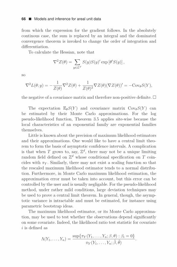
66 ! Models and inference for areal unit data
from which the expression for the gradient follows. In the absolutelycontinous case, the sum is replaced by an integral and the dominatedconvergence theorem is invoked to change the order of integration anddifferentiation.
To calculate the Hessian, note that
∇2Z(θ) =∑
y∈LT
S(y)S(y)′ exp [θ′S(y)] ,
so
∇2L(θ; y) = − 1Z(θ)∇2Z(θ) + 1
Z(θ)2 ∇Z(θ)(∇Z(θ))′ = −CovθS(Y ),
the negative of a covariance matrix and therefore non-positive definite. "
The expectation EθS(Y ) and covariance matrix CovθS(Y ) canbe estimated by their Monte Carlo approximations. For the logpseudo-likelihood function, Theorem 3.5 applies site-wise because thelocal characteristics of an exponential family are exponential familiesthemselves.
Little is known about the precision of maximum likelihood estimatorsand their approximations. One would like to have a central limit theo-rem to form the basis of asymptotic confidence intervals. A complicationis that when T grows to, say, Zd, there may not be a unique limitingrandom field defined on Zd whose conditional specification on T coin-cides with πY . Similarly, there may not exist a scaling function so thatthe rescaled maximum likelihood estimator tends to a normal distribu-tion. Furthermore, in Monte Carlo maximum likelihood estimation, theapproximation error must be taken into account, but this error can becontrolled by the user and is usually negligable. For the pseudo-likelihoodmethod, under rather mild conditions, large deviation techniques maybe used to prove a central limit theorem. In general, though, the asymp-totic variance is intractable and must be estimated, for instance usingparametric bootstrap ideas.
The maximum likelihood estimator, or its Monte Carlo approxima-tion, may be used to test whether the observations depend significantlyon some covariate. Indeed, the likelihood ratio test statistic for covariatei is defined as
Λ(Y1, . . . , Yn) = supπY (Y1, . . . , Yn; β, θ) : βi = 0πY (Y1, . . . , Yn; β, θ)
.
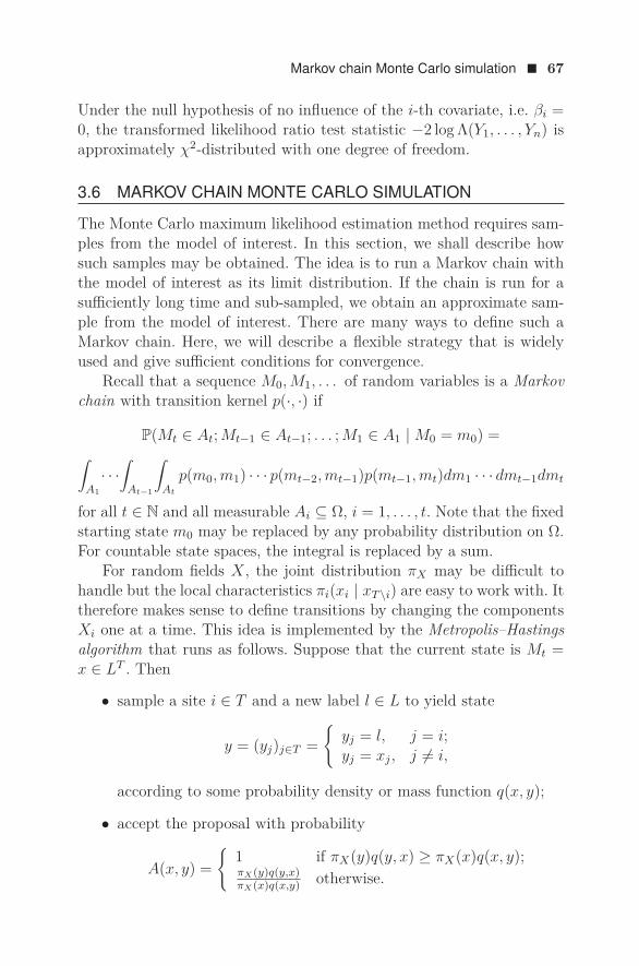
Markov chain Monte Carlo simulation ! 67
Under the null hypothesis of no influence of the i-th covariate, i.e. βi =0, the transformed likelihood ratio test statistic −2 log Λ(Y1, . . . , Yn) isapproximately χ2-distributed with one degree of freedom.
3.6 MARKOV CHAIN MONTE CARLO SIMULATION
The Monte Carlo maximum likelihood estimation method requires sam-ples from the model of interest. In this section, we shall describe howsuch samples may be obtained. The idea is to run a Markov chain withthe model of interest as its limit distribution. If the chain is run for asufficiently long time and sub-sampled, we obtain an approximate sam-ple from the model of interest. There are many ways to define such aMarkov chain. Here, we will describe a flexible strategy that is widelyused and give sufficient conditions for convergence.
Recall that a sequence M0, M1, . . . of random variables is a Markovchain with transition kernel p(·, ·) if
P(Mt ∈ At; Mt−1 ∈ At−1; . . . ; M1 ∈ A1 | M0 = m0) =∫
A1· · ·
∫
At−1
∫
At
p(m0, m1) · · · p(mt−2, mt−1)p(mt−1, mt)dm1 · · · dmt−1dmt
for all t ∈ N and all measurable Ai ⊆ Ω, i = 1, . . . , t. Note that the fixedstarting state m0 may be replaced by any probability distribution on Ω.For countable state spaces, the integral is replaced by a sum.
For random fields X, the joint distribution πX may be difficult tohandle but the local characteristics πi(xi | xT \i) are easy to work with. Ittherefore makes sense to define transitions by changing the componentsXi one at a time. This idea is implemented by the Metropolis–Hastingsalgorithm that runs as follows. Suppose that the current state is Mt =x ∈ LT . Then
• sample a site i ∈ T and a new label l ∈ L to yield state
y = (yj)j∈T =
yj = l, j = i;yj = xj , j = i,
according to some probability density or mass function q(x, y);
• accept the proposal with probability
A(x, y) =
1 if πX(y)q(y, x) ≥ πX(x)q(x, y);πX (y)q(y,x)πX (x)q(x,y) otherwise.
68 ! Models and inference for areal unit data
Note that the acceptance probabilities A(x, y) depend on the ratio
πX(y)πX(x) = πi(l | xT \i)
πi(xi | xT \i)
only. In particular, any normalising constants cancel out. The transitionkernel is obtained by combining the proposal and acceptance probabili-ties. In particular, p(x, y) = q(x, y)A(x, y) for x = y.
Proposition 3.2 Let X be an L-valued random field on a finite collec-tion T = ∅ of sites. Then the Metropolis–Hastings algorithm satisfies thefollowing properties:
• ‘detailed balance’
πX(x)p(x, y) = πX(y)p(y, x);
• πX is an invariant measure, that is, for all measurable A ⊆ LT ,
πX(X ∈ A) =∫
P(M1 ∈ A | M0 = x)πX(x)dx (L = R);
=∑
x
P(M1 ∈ A | M0 = x)πX(x) (L countable).
Proof: Without loss of generality, assume that x = y andπX(x)q(x, y) < πX(y)q(y, x). Then
πX(x)p(x, y) = πX(x)q(x, y) × 1
= πX(x)q(x, y)πX(y)q(y, x)πX(y)q(y, x)
= A(y, x)πX(y)q(y, x) = πX(y)p(y, x).
Invariance is a consequence of detailed balance. Indeed, for example inthe absolutely continuous case,
∫P(M1 ∈ A | M0 = x)πX(x)dx =
∫ (∫
Ap(x, y)πX(x)dy
)dx =
∫ (∫
Ap(y, x)πX(y)dy
)dx =
∫
AπX(y)
(∫p(y, x)dx
)dy =
∫
AπX(y)dy.
"
To study the convergence of the Metropolis–Hastings algorithm, re-call the following key definitions from Markov chain theory.

Markov chain Monte Carlo simulation ! 69
Definition 3.8 A Markov chain (Mt)t∈N0 on a countable state spaceΩ is irreducible if for all x, y ∈ Ω there exists some t ∈ N such thatP(Mt = y | M0 = x) > 0.
A Markov chain (Mt)t∈N0 with state space Ω = RT is πX-irreducibleif for all x ∈ Ω and all Borel sets A ⊂ RT for which πX(A) > 0 thereexists some t ∈ N such that P(Mt ∈ A | M0 = x) > 0.
The restriction to sets with positive probability is needed in the casethat Ω = RT , since in general the probability of returning to a singlestate will be zero. For πX -irreducible Markov chains, it is also possibleto define a concept of periodicity.
Definition 3.9 A πX-irreducible Markov chain (Mt)t∈N0 is aperiodic ifthere is no partition into non-empty measurable sets B0, . . . , Br−1, r ≥ 2,such that for all t ∈ N, P(Mt ∈ Bt mod r | M0 = x ∈ B0) = 1 and theunion of B0, . . . , Br−1 has πX-mass one.
We then have the following result.
Theorem 3.6 (Fundamental convergence theorem) If πX is aninvariant probability measure for a Markov chain (Mt)t∈N0 that is πX-irreducible and aperiodic, then Mt converges to πX in total variationfrom πX-almost all initial states, that is,
limt→∞
supA
|P(Mt ∈ A | M0 = x) − πX(A)| = 0
for πX-almost all x. The supremum is taken over all measurable sets.
Aperiodicity and irreducibility for the Metropolis–Hastings chain areinherited from those of the proposal distribution in the following sense.
Theorem 3.7 Let X be an L-valued random field on a finite collectionT = ∅ of sites and (Mt)t∈N0 a Metropolis–Hastings chain on Dπ = x ∈LT : πX(x) > 0. If the Markov chain governed by q is πX-irreducibleand q(x, y) = 0 ⇔ q(y, x) = 0, then (Mt)t∈N0 is πX-irreducible.
Proof: The condition that q(x, y) is zero precisely when q(y, x) is impliesthat the acceptance probabilities are strictly positive on Dπ.
Now, let (Qt)t∈N0 denote the Markov chain governed by the q(x, y)and denote its t-step transition kernel by qt. In other words, all proposedtransitions are accepted. We shall show by induction that qt(x, y) > 0implies pt(x, y) > 0, where pt is the t-step transition kernel of Mt.

70 ! Models and inference for areal unit data
To do so, let t = 1 and suppose that q(x, y) > 0 for x, y ∈ Dπ. Then,since A(x, y) > 0, also p(x, y) ≥ q(x, y)A(x, y) > 0. For the step from t tot + 1, suppose that qt+1(x, z) > 0 for some x and z in Dπ. Additionally,write St
p(x) for the support of pt(x, ·), Stq(x) for that of qt(x, ·), and
assume that Stq(x) ⊆ St
p(x). Since z ∈ St+1q (x) by assumption,
∫
Stp(x)
qt(x, y)q(y, z)dy ≥∫
Stq(x)
qt(x, y)q(y, z)dy > 0.
If z would not be an element of St+1p (x), then the support of the function
y 0→ pt(x, y)q(y, z) would be a null-set. By the induction assumption, thesupport of qt(x, ·)q(·, z) would also have measure zero in contradictionwith the above inequality.
Finally, for any A having positive πX -mass, since q is πX -irreducible,one may find a t ≥ 1 such that
P(Qt ∈ A | Q0 = x) =∫
Aqt(x, y)dy > 0.
By the induction result, also P(Mt ∈ A | M0 = x) > 0. "
As a corollary, suppose that Mt is πX -irreducible. Clearly, if there areself-transitions, P(Mt = Mt−1) > 0 for some t ∈ N, then Mt is aperiodic.Otherwise, if q is aperiodic, proposals do not cycle. The same is then truefor accepted proposals, implying the Metropolis–Hastings chain inheritsaperiodicity from q.
Example 3.10 In the context of Example 3.1, choose site and label uni-formly. More formally, q(x, y) = 1
2|T | for those x, y ∈ 0, 1T that differin at most one site. Then the proposal chain, and hence the Metropolis–Hastings sampler based on it, are irreducible and aperiodic.
3.7 HIERARCHICAL MODELLING
The goal of this section is to introduce the modern hierarchical modellingapproach by means of two concrete examples: image segmentation anddisease mapping.
3.7.1 Image segmentation
Suppose that one is not interested in all details of an image, but onlywishes to partition it into certain areas. For example, a cartographer

Hierarchical modelling ! 71
might want to classify the pixels in a satellite image according to its landuse. In another context, an oncologist may wish to distinguish betweenhealthy tissue and malignancies in a CT-scan of a patient.
Let x denote the target labelled image and y the vector of observedsignals. Each pixel value xi, i ∈ T , belongs to a finite class L of labels,the signals yi take values in some set S that is not necessarily identicalto L, and the goal is to reconstruct x from y.
In many applications it is reasonable to assume that, given the labels,the signals are conditionally independent and the signal at site i ∈ Tfollows a conditional probability density or mass function g(yi|xi) thatdepends only on the label xi at site i. Hence, for x ∈ LT , the forwardmodel becomes
f(y|x) =∏
i∈T
g(yi|xi), y ∈ ST .
The parameter of interest is the labelled image x. Its naive maximumlikelihood estimate x = X(y) based on the observed signal y is easy tocalculate:
xi = argmax g(yi|xi) : xi ∈ L, i ∈ T.
However, such estimators do not yield nice and smooth labellings becausethey completely ignore the spatial context. In other words, X = (Xi)i∈T
is sensitive to noise.To obtain more robust estimators, a Bayesian approach may be
taken. In addition to the forward model f(y|x), a prior distributionπX(x) is used that assigns low probability to images x that are roughin the sense of having small connected components. By Bayes’ rule, theposterior distribution of x given the data image y ∈ ST has probabilitymass function
f(x|y) ∝ f(y|x)πX(x) = πX(x)∏
i∈T
g(yi|xi), x ∈ LT .
Then, the maximum a posteriori estimator (MAP) X of X is chosenso as to maximise this posterior distribution. More specifically, if theobserved signal image is y, x = X(y) is given by
x = argmax f(y|x)πX(x) : x ∈ LT . (3.10)
This approach is also known as penalised maximum likelihood estimation,as optimising (3.10) is equivalent to maximising
log f(y|x) + log πX(x)

72 ! Models and inference for areal unit data
over all possible x. The first term log f(y|x) expresses the ‘goodness offit’ of x to the data, the second term the smoothness. Moreover, X isthe Bayes estimator (cf. Section 2.8) for the 0 − 1 loss function. To seethis, note that for any function X(·) of the random field Y ,
E [1X(Y ) = X] =∑
y∈ST
∑
x∈LT
1X(y) = xf(x|y)πY (y),
assuming S is countable. Otherwise, simply replace the sum over y byan integral. Therefore, upon observing Y = y, the Bayes estimator min-imises the posterior expectation
∑
x∈LT
1X(y) = xf(x|y)
and hence coincides with X.The role of the prior distribution is to encourage spatial coherence.
This can be achieved, for example, by a multi-label generalisation ofthe auto-logistic regression model of Example 3.1, which has probabilitymass function
πX(x) ∝ exp
⎡
⎣−θ∑
i∼j;i<j
1xi = xj
⎤
⎦ , x ∈ LT , (3.11)
for θ > 0. The model is known as the Potts model with label set L.Under the white noise assumption that the labels are observed subjectto independent zero-mean Gaussian noise with variance σ2, the posteriorprobability mass function given y ∈ RT is equal to
f(x|y) ∝ exp
⎛
⎝− 12σ2
∑
i∈T
(yi − xi)2 − θ∑
i∼j;i<j
1xi = xj
⎞
⎠ , x ∈ LT .
Direct computation of (3.10) is very difficult in general, but MonteCarlo ideas apply. Alternatively, and computationally faster, a local op-timum can be found in a greedy fashion by iterative pointwise optimi-sation:
xi = argmax g(yi|xi)πi(xi|xT \i) : xi ∈ L,
where the pixels i are visited in a systematic fashion, for example in rowmajor order. Since the computations are local, this method is very fast.However, the initial reconstruction may influence which local optimum

Hierarchical modelling ! 73
Figure 3.1 Segmentation of a noisy image of heather. From left to right:data image, MLE and MAP classifiers.
is reached so it is important to start well, for example in the maximumlikelihood estimate x.
As a simple illustration, the left-most panel of Figure 3.1 displays apattern of heather in Jadraas, Sweden, digitised at 100×200 pixels witha resolution of 10 pixels to the metre. The data was corrupted by whitenoise with variance σ2 = 15. The two right-most panels show greedyMAP-reconstructions for a Potts model with θ = 0 (corresponding tothe naive maximum likelihood estimator) and with θ = 25. In this case,using a prior reduces the misclassification error from five to one percent.
3.7.2 Disease mapping
The second example concerns spatially correlated count data arisingfrom small area sampling of some underlying process. For instance, alocal public health authority may be interested in the reported cases ofsome disease. For privacy reasons, these are typically aggregated overareas that are large enough to ensure that the counts cannot be tracedback to individuals. The goal of the analysis is to estimate the local dis-ease risk, perhaps based on spatial covariates such as pollution levels orcharacteristics of the population.
For counts, it is natural to assume a Poisson distribution and definea model in the spirit of the auto-logistic regression model. Thus, writ-ing Y for the vector of counts, the local characteristic at areal unit i

74 ! Models and inference for areal unit data
takes the form
πi(yi | yT \i) = e−µiµyii
yi!, yi ∈ N0,
withlog µi = αi + θ
∑j∼i,j =i
.
Since L = N0, we must verify that any putative joint distribution (3.2) iswell-defined, which turns out to be true only when θ is non-positive. Fornegative values of θ, when the regions surrounding i have high diseasecounts, the expected number of incidences in i itself will be low. Suchbehaviour is unrealistic for most diseases. Another disadvantage is thatthe logarithmic transform does not readily scale with respect to thesize of the areal units (the so-called ‘modifiable area unit’ or ‘changeof support’ problem). In conclusion, Poisson auto-regression models arenot suitable in the current context.
It is possible to model µi in terms of an integrated random field, butthe technical details are beyond the scope of this book. An alternative isto consider a mixture model for the rates µi directly. As usual, covariateinformation is captured by a design matrix X and parameter vectorβ ∈ Rp. Set, for α = Xβ,
µi = ci eαi ΛZi ,
where ci is a base rate of expected counts based on the population sizeof areal unit i and ΛZi is the area-specific relative risk. In a mixturemodel, random allocation variables Zi assign areal unit i to one of kmixture components λ1, . . . , λk ∈ R+. Spatial coherence can be achievedby assuming that (Zi)i∈T are distributed according to a Potts model(3.11). Provided that the covariates do not fluctuate too wildly, µi scalesappropriately with size.
The goal of a statistical analysis is to infer Z, or, equivalently, ΛZ , thespatial distribution of the relative risks, as well as the model parametersβ, θ and λ1, . . . , λk. In the nomenclature of the previous section, theforward model is
f(y|z; β, λ1, . . . , λk) =∏
i∈T
g(yi|(Xβ)i, λzi), y ∈ NT0 ,
with g(·|αi, λzi) the probability mass function of a Poisson distributionwith mean µi = cieαiλzi . The posterior probability mass function of theallocations conditional on the observed disease counts is
f(z|y; β, θ, λ1, . . . , λk) ∝ f(y|z; β, λ1, . . . , λk)πZ(z; θ), z ∈ 1, . . . , kT ,

Hierarchical modelling ! 75
for a proportionality constant that depends on the parameters. In a fullyBayesian framework, additional prior distributions may be placed on θ,the parameter of the Potts distribution πZ(·; θ), on β, on the mixturecomponents λj , j = 1, . . . , k, and even on k, leading to a joint distribu-tion of the form
f(y|z; β, λ1, . . . , λk)πZ(z; θ, k)p(λ1, . . . , λk|k)p(β)p(θ)p(k).
In any case, the posterior distribution can be approximated by MonteCarlo sampling and optimised numerically.
3.7.3 Synthesis
The two examples discussed in, respectively, Sections 3.7.1 and 3.7.2,share a common structure that can be found throughout spatial statis-tics. In both cases, a spatial process of interest – the pixel classificationin Section 3.7.1, the relative risks in Section 3.7.2 – cannot be observeddirectly, but only through other random variables (the noisy pixel valuesin Section 3.7.1, the counts in Section 3.7.2). Moreover, there may beunknown parameters. Thus, the joint distribution is of the form
forward model[data | process, parameters] × prior[process |parameters],
optionally complemented by a hyper prior distribution on the modelparameters. This framework is extremely flexible and may be adaptedto many different contexts.
Inference is usually based on the posterior distribution of the processand/or the parameters conditional on the observations, which can beapproximated by Monte Carlo methods. Sometimes a reconstruction ofthe process is required, as in the segmentation example. However, sincethe full posterior distribution is available, histograms of any marginaldistribution of interest can be plotted, e.g. the posterior distributionof the number of mixture components and allocation probabilities inthe disease mapping example. Further examples will be presented inChapter 3. In the meantime, we refer to Section 3.10 for pointers tomodern textbooks in this area.

76 ! Models and inference for areal unit data
3.8 WORKED EXAMPLES WITH R
The package spdep: Spatial dependence: Weighting schemes, statisticsand models can be used to find neighbourhood matrices and for esti-mating the parameters of Gaussian spatial autoregression schemes. Thepackage is maintained by R. Bivand. An up-to-date list of contributorsand a reference manual can be found on
https://CRAN.R-project.org/package=spdep.The results shown below were obtained using version 0.7-4.
Figure 3.2 Map of 49 districts in Columbus. The first district is indicatedby ‘+’.
The package contains a shape file ‘columbus.shp’ which includes apolygonal approximation of the borders of 49 neighbourhoods in thecity of Columbus, Ohio, in the United States of America as well as thecoordinates of their centroids in arbitrary digitising units. All sourcedata files were prepared by L. Anselin as described in his 1988 textbookSpatial Econometrics: Methods and Models. From now on, we assumethat the polygons have been extracted and stored in a data frame, saycolumbus.poly.
We are interested in the first of the Columbus neighbourhoods, whichis indicated by a cross in Figure 3.2. Be warned, though, that the labelsin the data frame are ”0” up to ”48”! The following script extracts thecentroids of the neighbourhoods and places a cross to indicate the neigh-bourhood of interest.plot(columbus.poly)columbus.centre <- coordinates(columbus.poly)
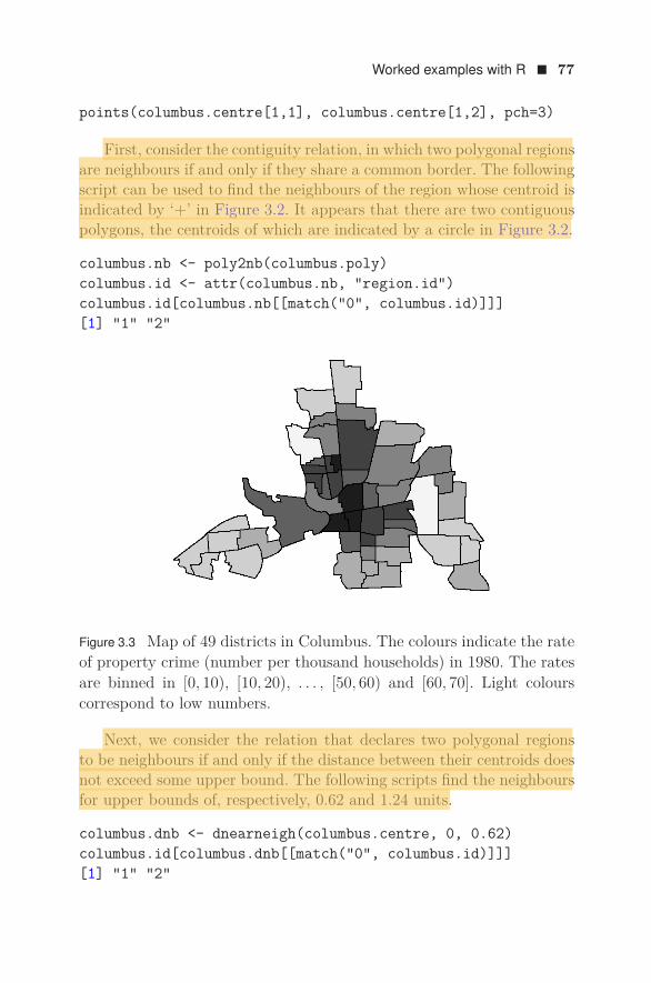
Worked examples with R ! 77
points(columbus.centre[1,1], columbus.centre[1,2], pch=3)
First, consider the contiguity relation, in which two polygonal regionsare neighbours if and only if they share a common border. The followingscript can be used to find the neighbours of the region whose centroid isindicated by ‘+’ in Figure 3.2. It appears that there are two contiguouspolygons, the centroids of which are indicated by a circle in Figure 3.2.
columbus.nb <- poly2nb(columbus.poly)columbus.id <- attr(columbus.nb, "region.id")columbus.id[columbus.nb[[match("0", columbus.id)]]][1] "1" "2"
Figure 3.3 Map of 49 districts in Columbus. The colours indicate the rateof property crime (number per thousand households) in 1980. The ratesare binned in [0, 10), [10, 20), . . . , [50, 60) and [60, 70]. Light colourscorrespond to low numbers.
Next, we consider the relation that declares two polygonal regionsto be neighbours if and only if the distance between their centroids doesnot exceed some upper bound. The following scripts find the neighboursfor upper bounds of, respectively, 0.62 and 1.24 units.
columbus.dnb <- dnearneigh(columbus.centre, 0, 0.62)columbus.id[columbus.dnb[[match("0", columbus.id)]]][1] "1" "2"
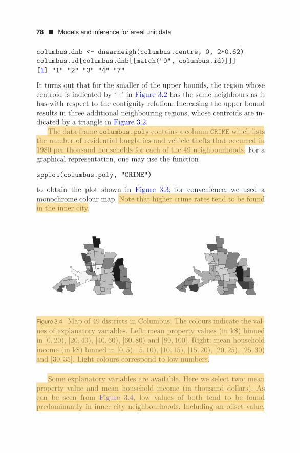
78 ! Models and inference for areal unit data
columbus.dnb <- dnearneigh(columbus.centre, 0, 2*0.62)columbus.id[columbus.dnb[[match("0", columbus.id)]]][1] "1" "2" "3" "4" "7"
It turns out that for the smaller of the upper bounds, the region whosecentroid is indicated by ‘+’ in Figure 3.2 has the same neighbours as ithas with respect to the contiguity relation. Increasing the upper boundresults in three additional neighbouring regions, whose centroids are in-dicated by a triangle in Figure 3.2.
The data frame columbus.poly contains a column CRIME which liststhe number of residential burglaries and vehicle thefts that occurred in1980 per thousand households for each of the 49 neighbourhoods. For agraphical representation, one may use the function
spplot(columbus.poly, "CRIME")
to obtain the plot shown in Figure 3.3; for convenience, we used amonochrome colour map. Note that higher crime rates tend to be foundin the inner city.
Figure 3.4 Map of 49 districts in Columbus. The colours indicate the val-ues of explanatory variables. Left: mean property values (in k$) binnedin [0, 20), [20, 40), [40, 60), [60, 80) and [80, 100]. Right: mean householdincome (in k$) binned in [0, 5), [5, 10), [10, 15), [15, 20), [20, 25), [25, 30)and [30, 35]. Light colours correspond to low numbers.
Some explanatory variables are available. Here we select two: meanproperty value and mean household income (in thousand dollars). Ascan be seen from Figure 3.4, low values of both tend to be foundpredominantly in inner city neighbourhoods. Including an offset value,

Worked examples with R ! 79
we may formulate a conditional autoregression model
Y = Xβ + B(Y − Xβ) + E
where Y = (Y1, . . . , Y49)′ denotes the random field of crime rates, X isthe 49 × 3 design matrix, B = φN is proportional to the neighbourhoodmatrix N and the 3 × 1 vector β contains parameters to be estimated.Specifically, all entries of the first column of X are 1, the second columnlists the mean property values, the third the average household incomes.Finally, E is spatially correlated noise with mean zero and covariancematrix σ2(I − B).
The following script fits the model by estimating its five parametersusing the contiguity neighbourhood relation: the components of β, φand σ2.
columbus.listw <- nb2listw(columbus.nb, style="B")car.out <- spautolm(formula= CRIME ˜ HOVAL + INC,
data=columbus.poly, listw=columbus.listw, family="CAR")columbus.poly$fitted.car <- fitted(car.out)
Figure 3.5 Map of 49 districts in Columbus. The colours indicate thefitted rate of property crime (number per thousand households) in 1980for a conditional autoregression model with contiguous neighbours. Therates are binned in [0, 10), [10, 20), . . . , [50, 60) and [60, 70]. Light colourscorrespond to low numbers.
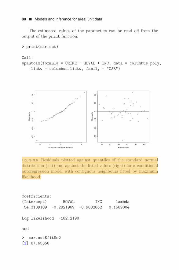
80 ! Models and inference for areal unit data
The estimated values of the parameters can be read off from theoutput of the print function:
> print(car.out)
Call:spautolm(formula = CRIME ˜ HOVAL + INC, data = columbus.poly,
listw = columbus.listw, family = "CAR")
−2 −1 0 1 2
−30
−20
−10
010
20
Quantiles of standard normal
Res
idua
ls
10 20 30 40 50 60
−30
−20
−10
010
20
Fitted values
Res
idua
ls
Figure 3.6 Residuals plotted against quantiles of the standard normaldistribution (left) and against the fitted values (right) for a conditionalautoregression model with contiguous neighbours fitted by maximumlikelihood.
Coefficients:(Intercept) HOVAL INC lambda54.3139189 -0.2821969 -0.9882862 0.1589004
Log likelihood: -182.2198
and
> car.out$fit$s2[1] 87.65356

Worked examples with R ! 81
In other words, φ = 0.16, σ = 9.36 and β = (54.31, −0.28, −0.99)′.We conclude that the model predicts less crime in affluent districts.The fitted model is displayed graphically in Figure 3.5. Note that it issmoother than the data due to the spatial averaging explicit in the modelformulation.
To validate the model, consider the residuals Y −Xβ − φN(Y −Xβ).If the model were correct, the residuals would be normally distributed.The QQ-plot
qqnorm(residuals(car.out))
indicates a deviation from normality due to a single negative outliercorresponding to neighbourhood ”6”. This conclusion is confirmed byplotting the residuals against the fitted values, cf. Figure 3.6. The outlieris clearly visible, but otherwise the plot shows no apparent trend.
Neighbourhood ”6” is the neighbourhood just west of the polygonswhose centroids are marked by a triangle in Figure 3.2. This particularneighbourhood enjoys a crime rate that is markedly smaller than thatof the surrounding neighbourhoods. Although property values there arerather high, the household incomes are not and after taking into ac-count the weighted averages over the surrounding neighbourhoods, thepredicted crime rate is higher than the actual one.
As an aside, note that realisations from the fitted model may eas-ily be obtained by adding multivariate normally distributed noise (withcovariance matrix σ2(I − φN)) to the fitted values.
The script for fitting a SAR model is similar to that for fitting aCAR model. Indeed,
sar.out <- spautolm(formula= CRIME ˜ HOVAL + INC,data=columbus.poly, listw=columbus.listw, family="SAR")
columbus.poly$fitted.sar <- fitted(sar.out)
results in
> print(sar.out)
Call:spautolm(formula = CRIME ˜ HOVAL + INC, data = columbus.poly,
listw = columbus.listw, family = "SAR")

82 ! Models and inference for areal unit data
Figure 3.7 Map of 49 districts in Columbus. The colours indicate thefitted rate of property crime (number per thousand households) in 1980for a simultaneous autoregression model with contiguous neighbours.The rates are binned in [0, 10), [10, 20), . . . , [50, 60) and [60, 70]. Lightcolours correspond to low numbers.
Coefficients:(Intercept) HOVAL INC lambda56.3315730 -0.2998181 -0.9515649 0.1211682
Log likelihood: -182.5554
and
> sar.out$fit$s2[1] 91.43706
In other words, φ = 0.12, σ = 9.56 and β = (56.33, −0.30, −0.95)′.A comparison of Figures 3.5 and 3.7 shows that the two models han-dle sharp discontinuities in the data somewhat differently; in such casesthe fitted crime rates under the conditional autoregression seem a lit-tle smoother. The diagnostic plots shown in Figure 3.8 suggest the fitis slightly worse for a simultaneous autoregression but still adequate,except for neighbourhood ”6”.

Worked examples with R ! 83
−2 −1 0 1 2
−30
−20
−10
010
20
Quantiles of standard normal
Res
idua
ls
10 20 30 40 50 60
−30
−20
−10
010
20
Fitted valuesR
esid
uals
Figure 3.8 Residuals plotted against quantiles of the standard normaldistribution (left) and against the fitted values (right) for a simultaneousautoregression model with contiguous neighbours fitted by maximumlikelihood.

84 ! Models and inference for areal unit data
3.9 EXERCISES
1. Consider the hard core lattice gas X on a finite grid ∅ = T ⊂ Z2
with value set L = 0, 1. Write i ∼ j whenever 0 < ||i − j|| ≤ 1so that sites i and j are neighbours when they are horizontally orvertically adjacent. The probability mass function is, for x ∈ LT ,defined by
πX(x) = 1
Z
∏i∈T axi if xixj = 0 whenever i ∼ j;
0 otherwise.
Here a > 0 and Z is a normalising constant.
• Compute the local characteristics.• Order the sites in T lexicographically. Show that there ex-
ist x = (xi)i∈T , y = (yi)i∈T and i ∈ T such that πi(yi |xj:j<i, yj:j>i) is zero but both πX(x) and πX(y) are posi-tive.
2. In a conditional autoregression model, show that bij = 0 impliesthat Xi and Xj are conditionally independent given (Xt)t∈T \i,j.Are Xi and Xj independent?Hint: Recall that if A is a symmetric, non-singular block matrix
A =[
I A12A21 = A′
12 A22
]
,
then its inverse is given by[
I + A12(A22 − A21A12)−1A21 −A12(A22 − A21A12)−1
−(A22 − A21A12)−1A21 (A22 − A21A12)−1
]
.
3. Show that the local characteristics
π1(x | y) = π2(y | x) = 1(2π)1/2 exp
[−1
2(x − y)2]
do not define a proper joint distribution on R1,2.
4. Suppose that T is a finite set equipped with a symmetric relation∼ which contains at least two ∼-related elements. Show that thePoisson auto-regression model with putative local characteristics
πi(yi | yT \i) = e−µiµyi
i /yi!log µi = θ
∑j∼i,j =i yj
for y ∈ NT0 is well-defined if and only if θ ≤ 0.

Exercises ! 85
5. Consider the conditional autoregression model on a finite fam-ily T = ∅ of sites defined by Gaussian local characteristics withVar(Xt | XT \t) = 1 and
E(Xt | XT \t) = µ +∑
s =t
bts(Xs − µ), t ∈ T,
for some unknown parameter µ ∈ R. Propose a two-sided testfor the hypothesis that µ = 0. What assumptions do you need toimpose on the bts?
6. Show that the potential in Example 3.5 is normalised with respectto a = 0.
7. Suppose that T is a finite set that contains at least two elementsand is equipped with a symmetric relation ∼. For the Poissonauto-regression model defined by
πi(yi | yT \i) = e−µiµyi
i /yi!log µi = −
∑j∼i,j =i yj
for y ∈ NT0 , i ∈ T , find the canonical potential with respect to
a = 0.
8. Let ∅ = T ⊂ Z2 be a finite grid. For i = j ∈ T , write i ∼ j if andonly if 0 < ||i − j|| ≤ 1. Show that if X is a Markov random fieldon T with respect to ∼, then the ‘x’ sites in the following pictureare conditionally independent given the ‘o’ sites:
x o x o x o xo x o x o x ox o x o x o xo x o x o x ox o x o x o xo x o x o x ox o x o x o x
9. Let ∼ be a symmetric relation on the finite set ∅ = T and considera conditional autoregression model on RT defined by a square non-singular matrix B whose diagonal entries are zero and a diagonalmatrix K with positive entries κi on the diagonal such that (I −B)−1K is positive definite.

86 ! Models and inference for areal unit data
Suppose that the entries bij of the matrix B satisfy the propertythat bij = 0 if i ∼ j, i, j ∈ T . Show that this model is a Markovrandom field with respect to ∼ and find an explicit expression forthe interaction functions.
10. Consider the hard core lattice gas X on a finite grid ∅ = T ⊂ Z2
with value set L = 0, 1 and probability mass function
πX(x) = 1
Z(a)∏
i∈T axi if xixj = 0 whenever i ∼ j
0 otherwise
for a > 0 and x ∈ LT . Here i ∼ j whenever 0 < ||i−j|| ≤ 1. Designa suitable Monte Carlo method for approximating the maximumlikelihood estimator of a. Prove its convergence.
11. Consider the model
Y = Xβ + B(Y − Xβ) + E
where X is an n×p design matrix, β ∈ Rp an unknown parameter,B an n × n symmetric positive definite matrix with zero elementson the diagonal and E normally distributed with mean zero andcovariance matrix σ2(I −B) for unknown parameter σ2 > 0. Com-pute the maximum pseudo-likelihood estimators for the parame-ters β and σ2. Compare your answer to the maximum likelihoodestimators β and σ2.
12. Suppose that the random field X on a finite index set T = ∅ isdefined by the probability mass function
πX(x) = eθS(x)
Z(θ) , x ∈ 0, 1T ,
for some function S : 0, 1T → R. Given a realisation x ∈ 0, 1T ,show that the maximum pseudo-likelihood estimator θ satisfies
1|T |
∑
i∈T
Eθ [S(X) | Xj = xj , j = i] = S(x).
13. Let πX > 0 be a probability distribution on LT for non-emptyfinite sets L and T . Consider the Metropolis–Hastings algorithmwith proposal distribution
q(x, y) =∑
i∈T
1|T |πi(yi | xT \i)1yT \i = xT \i, x, y ∈ LT .

Exercises ! 87
Show that all proposals for which q(x, y) > 0 are accepted withprobability one.
14. Consider the greedy algorithm for the Gaussian–Potts model usedto obtain Figure 3.1. Describe the updates for θ = 0 and θ → ∞.
15. The spdep package contains a data set nc.sids which containsinformation on the number of births as well as the number of deathsfrom Sudden Infant Death Syndrome in counties in North Carolina.Fit an appropriate auto-binomial model.

88 ! Models and inference for areal unit data
3.10 POINTERS TO THE LITERATURE
The mathematical theory of Markov random fields was developed in the1960s, although specific examples had been studied before. For instance,the Ising model originates from the 1924 graduate thesis of E. Ising[1] under supervision of W. Lenz [2]. An early paper on a Gaussianautoregression is [3] by P. Whittle (1954).
Besag’s factorisation theorem occurs as (2.2) in [4] building on workby D. Brook [5]. Indeed, Brook appears to be the first author to studyconsistency conditions for conditional specifications. The name Markovrandom field was coined by P.L. Dobrushin for random fields defined oninfinite lattices that satisfy a spatial Markov property with respect toa distance based relation [6]. Section 4 of [4] is concerned with spatialautoregression models including the auto-logistic regression of Exam-ple 3.1, and the Gaussian models of Section 3.2. Proposition 3.1 andlikelihood based inference can be found in section 5.2 of B.D. Ripley’spioneering textbook in spatial statistics [7].
Gibbs states are named after J.W. Gibbs, the founder of modern sta-tistical physics. The proof of Theorems 3.2 and 3.4 based on the Mobiusinversion theorem of G.-C. Rota [8, Proposition 3.2] is due to G.R. Grim-mett [9]. Alternative proofs can be found in the paper by J. Moussouris[10]. Example 3.9 is also taken from this paper. The Hammersley–Cliffordtheorem was named after J.M. Hammersley and P.E. Clifford [11] by J.E.Besag [4, Section 3], who also noted the equivalence of local and spatialMarkov properties established in Corollary 3.2.
For more details on Markov random fields, we refer the reader to thetextbooks by Kinderman and Snell [12] and Y.A. Rozanov [13], or themore recent one by X. Guyon [14]. For an introduction to the wider classof graphical models, one may consult S.L. Lauritzen’s monograph [15].
Gaussian autoregression models are discussed in great detail in [16].The R-package spdep can be used to fit such models to data. Alterna-tively, the R-INLA package maintained by H. Rue may be used.
For random field models with an intractable likelihood, J.E. Besagproposed to use maximum pseudo-likelihood estimation instead [17] andshowed that for CAR models, the technique reduces to least squaresestimation. The Monte Carlo maximum likelihood method in the formpresented here is due to Geyer and Thompson [18] and Theorem 3.5 istaken from this paper.
The study of stochastic processes in which the future and the pastare conditionally independent given the present was inspired by A.A.

References ! 89
Markov’s 1913 study of the succession of vowels and consonants in theclassic novel Eugene Onegin by Pushkin. An excellent introduction tothe theory of such Markov chains on general state spaces is given in thetextbook by Meyn and Tweedie [19]. Our definition in terms of transitionprobability kernels can be found in section 3.4 of the second edition.The concept of πX -irreducibility dates back to W. Doeblin [20, 21]
and is discussed in chapter 4 of [19]. Cycles were also considered byDoeblin [21]. The consideration of ergodic theorems for Markov chainswith finite state space is already found in work by A.N. Kolmogoroff [22],who used contraction principles and differential equations. The proof forgeneral state spaces may be based on techniques from E. Nummelin [23],a coherent account of which is given in [19, Section 13]. Theorem 3.7 isdue to Roberts and Smith [24, Theorem 3].
From a computational point of view, the Metropolis–Hastings algo-rithm was introduced in the paper by Metropolis, the Rosenbluths andthe Tellers [25] and is a special case of a class of methods proposed byW.K. Hastings [26], designed to satisfy the detailed balance equations inProposition 3.2. For an exhaustive overview of these and other Markovchain Monte Carlo techniques and their applications, we refer the readerto the Handbook edited by Brooks, Gelman, Jones and Meng [27].
The modern hierarchical modelling approach to image analysis, andto spatial statistics in general, can be traced back to J.E. Besag’s note[28] and seminal paper [29] and to the pioneering work by the Gemanbrothers [30]. Textbooks on this topic include G. Winkler’s monograph[31] on Bayesian image analysis and the more general volume by Baner-jee, Carlin and Gelfand [32]. In particular, the segmentation example isinspired by [29] which also contains the greedy iterative pointwise opti-misation algorithm. The heather data that we used as an illustration wascollected by P.J. Diggle [33] and is available in the R-package spatstat.The prior Potts model was introduced in R.B. Potts’ doctoral thesis [34].Finally, our account of disease mapping is inspired by a paper by Greenand Richardson [35]. Further details and alternative modelling strategiescan be found in chapter 14 of the Handbook of Spatial Statistics [36].
REFERENCES
[1] E. Ising (1924). Beitrag zur Theorie des Ferro- und Paramagnetismus. PhDthesis, University of Hamburg.
[2] W. Lenz (1920). Beitrage zum Verstandnis der magnetischen Eigenschaften infesten Korpern. Physikalische Zeitschrift 21:613–615.

90 ! Models and inference for areal unit data
[3] P. Whittle (1954). On stationary processes in the plane. Biometrika41(3/4):434–449.
[4] J.E. Besag (1974). Spatial interaction and the statistical analysis of latticesystems. Journal of the Royal Statistical Society B36(2):192–236.
[5] D. Brook (1964). On the distinction between the conditional probability andthe joint probability approaches in the specification of nearest-neighboursystems. Biometrika 51(3/4):481–483.
[6] P.L. Dobrushin (1968). The description of a random field by means of condi-tional probabilities and conditions of its regularity. Theory of Probabilityand its Applications, 13(2):197–224.
[7] B.D. Ripley (1981). Spatial Statistics. New York: John Wiley & Sons.
[8] G.-C. Rota (1964). On the foundations of combinatorial theory I. Theoryof Mobius functions. Zeitschrift fur Wahrscheinlichkeitstheorie und Ver-wandte Gebiete 2(4):340–368.
[9] G.R. Grimmett (1973). A theorem about random fields. Bulletin of the LondonMathematical Society 5(1):81–84.
[10] J. Moussouris (1974). Gibbs and Markov random systems with constraints.Journal of Statistical Physics 10(1):11–33.
[11] J.M. Hammersley and P.E. Clifford (1971). Markov fields on finite graphs andlattices. Unpublished manuscript.
[12] R. Kinderman and J.L. Snell (1980). Markov Random Fields and Their Ap-plications. Providence, Rhode Island: American Mathematical Society.
[13] Y.A. Rozanov (1982). Markov Random Fields. New York: Springer-Verlag.
[14] X. Guyon (1995). Random Fields on a Network: Modeling, Statistics, and Ap-plications. New York: Springer-Verlag.
[15] S.L. Lauritzen (1996). Graphical Models. Oxford: Oxford University Press.
[16] H. Rue and L. Held (2005). Gaussian Markov Random Fields. Theory andApplications. Boca Raton, Florida: Chapman & Hall/CRC.
[17] J. Besag (1975). Statistical analysis of non-lattice data. Journal of the RoyalStatistical Society D24(3):179–195.
[18] C.J. Geyer and E.A. Thompson (1992). Constrained maximum likelihood fordependent data. Journal of the Royal Statistical Society B54(3):657–699.
[19] S. Meyn and R.L. Tweedie (2009). Markov Chains and Stochastic Stability(2nd edition). Cambridge: Cambridge University Press.
References ! 91
[20] W. Doeblin (1937). Sur les proprietes asymptotiques de mouvement regis parcertain types de chaınes simples. Bulletin Mathematique de la SocieteRoumaine des Sciences 39(1):57–115; 39(2):3–61.
[21] W. Doeblin (1940). Elements d’une theorie generale des chaınes simples con-stantes de Markoff. Annales Scientifiques de l’Ecole Normale Superieure57(3):61–111.
[22] A. Kolmogoroff (1931). Uber die analytischen Methoden in der Wahrschein-lichkeitsrechnung. Mathematische Annalen 104(1):415–458.
[23] E. Nummelin (1984). General Irreducible Markov Chains and Non-negativeOperators. Cambridge: Cambridge University Press.
[24] G.O. Roberts and A.F.M. Smith (1994). Simple conditions for the conver-gence of the Gibbs sampler and Metropolis–Hastings algorithms. Stochas-tic Processes and Their Applications 49(2):207–216.
[25] N. Metropolis, A.W. Rosenbluth, M.N. Rosenbluth, A.H. Teller and E. Teller(1953). Equation of state calculations by fast computing machines. Jour-nal of Chemical Physics 21(6):1087–1092.
[26] W.K. Hastings (1970). Monte Carlo sampling methods using Markov chainsand their application. Biometrika 57(1):97–109.
[27] S. Brooks, A. Gelman, G.L. Jones and X.-L. Meng, editors (2011). Hand-book of Markov Chain Monte Carlo. Boca Raton, Florida: Chapman &Hall/CRC.
[28] J.E. Besag (1983). Discussion of paper by P. Switzer. Bulletin of the Interna-tional Statistical Institute 50(3):422–425.
[29] J.E. Besag (1986). On the statistical analysis of dirty pictures (with discus-sion). Journal of the Royal Statistical Society B48(3):259–302.
[30] S. Geman and D. Geman (1984). Stochastic relaxation, Gibbs distributions,and the Bayesian restoration of images. IEEE Transactions on PatternAnalysis and Machine Intelligence 6(6):721–741.
[31] G. Winkler (2003). Image Analysis, Random Fields and Markov ChainMonte Carlo Methods. A Mathematical Introduction (2nd edition). Berlin:Springer-Verlag.
[32] S. Banerjee, B.P. Carlin and A.E. Gelfand (2015). Hierarchical Modeling andAnalysis for Spatial Data (2nd edition). Boca Raton, Florida: Chapman& Hall/CRC.
[33] P.J. Diggle (1981). Binary mosaics and the spatial pattern of heather. Biomet-rics 37(3):531–539.

92 ! Models and inference for areal unit data
[34] R.B. Potts (1951). The mathematical investigation of some cooperative phe-nomena. D.Phil. thesis, University of Oxford.
[35] P.J. Green and S. Richardson (2002). Hidden Markov models and disease map-ping. Journal of the American Statistical Association 97(460):1055–1070.
[36] A.E. Gelfand, P.J. Diggle, M. Fuentes and P. Guttorp, editors (2010). Hand-book of Spatial Statistics. Boca Raton, Florida: Chapman & Hall/CRC.

C H A P T E R 4
Spatial point processes
4.1 POINT PROCESSES ON EUCLIDEAN SPACES
Up to now, data were collected at fixed locations or regions. Sometimes,however, the locations at which events occur are random. Typical ex-amples include the epicentres of earthquakes or the outbreaks of forestfires. Such random configurations of locations are said to form a pointprocess.
To exclude pathological cases, the following definition will be needed.
Definition 4.1 The family N lf(Rd) of locally finite point configurationsin Rd consists of all subsets x ⊂ Rd that place finitely many points inevery bounded Borel set A ⊂ Rd.
In particular, locally finite configurations are at most countably in-finite and do not contain accumulation points. It is possible to find twopoints at exactly the same location, though.
Definition 4.2 A point process X ∈ N lf(Rd) on Rd is a random locallyfinite configuration of points such that for all bounded Borel sets A ⊂ Rd
the number of points of X that fall in A is a finite random variable whichwe shall denote by NX(A).
Example 4.1 Let W be a bounded Borel set in Rd having positive d-volume |W | > 0, and, for n ∈ N, let X1, . . . , Xn be independent anduniformly distributed on W . Then, X = X1, . . . , Xn is the binomialpoint process. Indeed,
NX(A) =n∑
i=11Xi ∈ A ≤ n
93

94 ! Spatial point processes
is a finite random variable for every Borel set A ⊆ W .
As for the random fields studied in Chapter 2, the distribution of apoint process is completely specified by the finite dimensional distribu-tions (fidi’s)
P(NX(A1) = n1; · · · ; NX(Am) = nm).Here, for m ∈ N, i = 1, . . . , m, the Ai ⊂ Rd are bounded Borel sets andni ∈ N0.
Example 4.2 Consider the binomial point process of Example 4.1. LetA, B be two Borel subsets of W . Note that A and B partition W in fourdisjoint subsets, A ∩ B, A \ B, B \ A and the complement of A ∪ B. Theuniform distribution of the Xi implies that the probability of falling inA∩B is |A∩B|/|W |, with similar expressions for the hitting probabilitiesof the other three sets. Therefore,
P(NX(A \ B) = n1; NX(B \ A) = n2; NX(A ∩ B) = n3)
= n!n1!n2!n3!(n −
∑i ni)!
( |A \ B||W |
)n1 ( |B \ A||W |
)n2 ( |A ∩ B||W |
)n3
×
×(
1 − |A ∪ B||W |
)n−∑
ini
.
Summation over appropriate values of n1, n2, n3 yields an explicit ex-pression for P(NX(A) = nA; NX(B) = nB).
The fidi’s are not very tractable, even for the binomial point processconsidered above. However, if one assumes that the point process X issimple in the sense that its realisations almost surely do not containmultiple points at exactly the same location, it suffices to consider onlythe one-dimensional fidi’s.
Theorem 4.1 The distribution of a simple point process X on Rd iscompletely determined by the void probabilities
v(A) = P(NX(A) = 0)
of bounded Borel sets A ⊂ Rd.

Point processes on Euclidean spaces ! 95
Proof: Define a family of difference operators Sk(·; A1, . . . , Ak) indexedby bounded Borel sets A1, . . . , Ak, k ∈ N, inductively as follows:
S1(B; A1) = v(B) − v(A1 ∪ B)
and
Sk(B; A1, . . . , Ak) = Sk−1(B; A1, . . . , Ak−1)−Sk−1(B∪Ak; A1, . . . , Ak−1),
where B ⊂ Rd is a bounded Borel set. Note that
Sk(B; A1, . . . , Ak) = P(NX(Ai) > 0, i = 1, . . . , k; NX(B) = 0)
depends only on events that record presence or absence of points andhence is completely determined by the void probabilities.
By the topological properties of the Euclidean space Rd, there existsa series of nested partitions Tn,i, i = 0, . . . , kn, such that for large ndistinct points x, y ∈ Rd lie in different members of (Tn,i)i. Here n is thelevel in the nesting and i ranges through the members of the partitionat level n. For any bounded Borel set A ⊂ Rd, intersection with themembers of the partition results in a nested partition of A that separatesthe points, so the limit
limn→∞
∑
i
1NX(A ∩ Tni) > 0 = NX(A)
exists almost surely. Here we use the fact that X is simple!The joint distribution of the random variables 1NX(A ∩ Tn,i), i =
0, . . . , kn, can be expressed in terms of the difference operators. Indeed,since indicator variables take binary values only, for ij ∈ 0, 1,
P(1NX(A ∩ Tn,0) > 0 = i0; · · · ; 1NX(A ∩ Tn,kn) > 0 = ikn)
= Sl(∪j:ij=0(A ∩ Tn,j); A ∩ Tn,j , ij = 1)where l = ∑
j 1ij = 1. Hence, writing Hn(A) = ∑i 1NX(A ∩ Tn,i) >
0, the probability that Hn(A) takes the value l is equal to∑
P(1NX(A ∩ Tn,0) > 0 = i0; · · · ; 1NX(A ∩ Tn,kn) > 0 = ikn),
where the sum is taken over all combinations of ijs that sum to l ∈ N0.Thus, P(Hn(A) = l) can be expressed solely in terms of the differenceoperators and hence in terms of the void probabilities. A similar rea-soning applies to the joint distribution of (Hn(A1), . . . , Hn(Ak)) for anyk ∈ N. Letting n increase to infinity completes the proof. "

96 ! Spatial point processes
Example 4.3 Let W be a bounded Borel set in Rd having positived-volume |W | > 0. For the binomial process on W (cf. Example 4.1),the void probability of a bounded Borel set A ⊂ Rd is
v(A) = (1 − |A ∩ W |/|W |)n .
To conclude this section, we present a constructive way to definefinite point patterns, namely to specify
• a discrete probability distribution (pn)n∈N0 for the total number ofpoints;
• a family of symmetric joint probability densities jn(x1, . . . , xn),n ∈ N, on (Rd)n for the locations of the points given that thereare n of them.
Example 4.4 For the binomial process of Example 4.1, pn = 1 andpm = 0 for m = n. Moreover, jn ≡ |W |−n is symmetric.
4.2 THE POISSON PROCESS
Recall that the Poisson distribution arises as the limit of binomial distri-butions with ever more trials having ever smaller success probabilities.The same idea applies to binomial point processes.
To be specific, fix k ∈ N0 and let Bn ⊂ Rd be a series of growing ballscentred at the origin such that n/|Bn| ≡ λ is constant (0 < λ < ∞).Then any bounded Borel set A is covered by Bn for n ≥ k sufficientlylarge, and, in this case,
P(n)(N(A) = k) =(
n
k
) ( |A||Bn|
)k (1 − |A|
|Bn|
)n−k
,
where the notation P(n) is used for the distribution of the binomial pointprocess of n points in Bn. Under the assumptions on n and Bn,
P(n)(N(A) = k) → e−λ|A| (λ|A|)k
k!as n → ∞. Similarly, for disjoint bounded Borel sets A and B andk, l ∈ N0,
P(n)(N(A) = k; N(B) = l) =(
n
k
) ( |A||Bn|
)k(
n − k
l
) ( |B||Bn|
)l
×(
1 − |A ∪ B||Bn|
)n−k−l

The Poisson process ! 97
for n ≥ k + l large enough for Bn to cover A ∪ B. As n → ∞, the limit
limn→∞
P(n)(N(A) = k; N(B) = l) = e−λ|A| (λ|A|)k
k! e−λ|B| (λ|B|)l
l!is a product of Poisson probabilities with parameters λ|A| and λ|B|,respectively.
The above calculations suggest the following definition.
Definition 4.3 A point process X on Rd is a homogeneous Poissonprocess with intensity λ > 0 if
• NX(A) is Poisson distributed with mean λ|A| for every boundedBorel set A ⊂ Rd;
• for any k disjoint bounded Borel sets A1, . . . , Ak, k ∈ N, the ran-dom variables NX(A1), . . . , NX(Ak) are independent.
The void probabilities of a Poisson process are given by
v(A) = exp [−λ|A|] .
At this point, it should be mentioned that the second property inthe definition above is crucial and implies that the restrictions of X todisjoint sets behave independently. The first property may be relaxed inthe sense that λ|A| may be replaced by
∫
Aλ(x)dx (4.1)
for some function λ : Rd → R+ that is integrable on bounded sets but notnecessarily constant. The resulting point process is an inhomogeneousPoisson process.
Theorem 4.2 Let X be a homogeneous Poisson process on Rd withintensity λ > 0 and A ⊂ Rd a bounded Borel set with |A| > 0. Then,conditional on the event NX(A) = n, n ∈ N, the restriction of X toA is a binomial point process of n points.
Proof: Let B ⊂ A be a bounded Borel set. Its conditional void proba-bility is given by
P(NX(B) = 0|NX(A) = n) = P(NX(B) = 0; NX(A) = n)P(NX(A) = n)
98 ! Spatial point processes
= P(NX(B) = 0; NX(A \ B) = n)P(NX(A) = n) = e−λ|B|e−λ|A\B|(λ|A \ B|)n/n!
e−λ|A|(λ|A|)n/n!
=( |A \ B|
|A|
)n
,
since NX(B) and NX(A \ B) are independent and Poisson distributedwith rates λ|B| and λ|A \ B|, respectively. Note that the conditionalvoid probability of B is equal to the corresponding void probability ofthe binomial point process (cf. Example 4.3). Therefore, an appeal toTheorem 4.1 concludes the proof. "
As a corollary, observe that the joint probability densities jn of aPoisson process on a bounded window A coincide with those of the bi-nomial point process.
4.3 MOMENT MEASURES
The moments, especially the first two, are important descriptors of ran-dom variables, as are the mean and covariance functions of random fields.For point processes, their analogues are the moment measures.
Definition 4.4 Let X be a point process on Rd. Define, for Borel setsA, B ⊆ Rd,
α(1)(A) = ENX(A);µ(2)(A × B) = E [NX(A)NX(B)] ;
α(2)(A × B) = E
⎡
⎣∑
x∈X
∑ =
y∈X
1x ∈ A; y ∈ B
⎤
⎦ .
Here, the notation ∑ = is used to indicate that the sum is taken over all(x, y) ∈ X2 for which x = y.
The set functions introduced in Definition 4.4 are not necessarilyfinite, even for finite point processes. To see this, let, for example, thenumber of points be governed by the probability density (pn)n withpn = 1/(n(n − 1)) for n ≥ 2 and zero otherwise. Then the pn sum toone, but the expected total number of points is infinite. For finite pointprocesses, a sufficient condition for µ(2) and, a fortiori, α(1) and α(2) totake finite values is that E
[NX(Rd)2]
< ∞. More generally, providedthat they take finite values on bounded Borel sets, classic results from

Moment measures ! 99
measure theory imply that these set functions can be extended to unique(σ-finite) Borel measures which are necessarily symmetric.
Definition 4.5 Suppose that the set functions defined in Definition 4.4are finite for bounded Borel sets. Then they can be uniquely extended tosymmetric Borel measures. The resulting measures α(k), k = 1, 2, arethe k-th order factorial moment measures of X, whereas the extensionof µ(2) will be referred to as the second order moment measure.
In fact, for every α(k)-integrable function f : (Rd)k → R,
E
⎡
⎣∑ =
(x1,...,xk)∈Xk
f(x1, . . . , xk)
⎤
⎦ =∫
· · ·∫
f(x1, . . . , xk)dα(k)(x1, . . . , xk).
(4.2)
Example 4.5 Let X be a Poisson process on Rd with intensity functionλ. Then, by definition, NX(A) is Poisson distributed with expectationΛ(A) =
∫A λ(x)dx < ∞ for every bounded Borel set A. Hence, α(1)(A) =
Λ(A).To compute the second order moment measure, use the fact that the
counts in disjoint sets are independent to write, for bounded Borel setsA, B ⊂ Rd,
µ(2)(A × B) = E [N(A)N(A ∩ B) + N(B \ A)]= E [N(A ∩ B) + N(A \ B)N(A ∩ B)] + Λ(A)Λ(B \ A)= Λ(A ∩ B) + Λ(A ∩ B)2 + Λ(A \ B)Λ(A ∩ B) + Λ(A)Λ(B \ A)= Λ(A ∩ B) + Λ(A ∩ B) [Λ(A ∩ B) + Λ(A \ B)] + Λ(A)Λ(B \ A)
=∫
A
∫
Bλ(x)λ(y)dxdy +
∫
A∩Bλ(x)dx.
Sinceµ(2)(A × B) = α(2)(A × B) + α(1)(A ∩ B),
the second order factorial moment measure is
α(2)(A × B) =∫
A
∫
Bλ(x)λ(y)dxdy.
In the current context, the covariance is defined in terms of the firsttwo moments as follows:
Cov(NX(A), NX(B)) = µ(2)(A × B) − α(1)(A)α(1)(B).

100 ! Spatial point processes
Definition 4.6 Let X be a point process on Rd. If the factorial momentmeasure α(k) exists and admits a density in the sense that
α(k)(A1 × · · · × Ak) =∫
A1· · ·
∫
Ak
ρ(k)(x1, . . . , xk)dx1 · · · dxk
for all Borel sets A1, . . . , Ak, then ρ(k) is the k-th order product density,k = 1, 2.
Intuitively speaking, ρ(k)(x1, . . . , xk)dx1 · · · dxk is the infinitesimalprobability of finding points of X at regions dx1, . . . , dxk aroundx1, . . . , xk.
Example 4.6 Let X be a Poisson process on Rd with intensity func-tion λ. Then, for x, y ∈ Rd, ρ(1)(x) = λ(x) and ρ(2)(x, y) =λ(x)λ(y). When well-defined, the pair correlation function g(x, y) =ρ(2)(x, y)/(ρ(1)(x)ρ(1)(y)) ≡ 1, reflecting the lack of correlation betweenpoints of X.
4.4 STATIONARITY CONCEPTS AND PRODUCT DENSITIES
In this section, we consider estimation of the product densities of a spa-tial point process. In order to do so, some stationarity concepts will beneeded.
Definition 4.7 A point process X on Rd is stationary if for all boundedBorel sets A1, . . . , Ak in Rd, all n1, . . . , nk in N0 and all s ∈ Rd,
P(NX(s + A1) ≤ n1; . . . ; NX(s + Ak) ≤ nk) = P(NX(A1) ≤ n1;. . . ; NX(Ak) ≤ nk).
In other words, the distribution of X is invariant under translations.A fortiori, the same is true for the moment measures of X provided thatthey exist. A weaker property that allows some spatial variation is thefollowing.
Definition 4.8 Let X be a point process on Rd for which the first andsecond order factorial moment measures exist and admit a product den-sity ρ(k), k = 1, 2. Then X is said to be second order intensity-reweightedmoment stationary if
ρ(1)(x) ≥ ρmin > 0

Stationarity concepts and product densities ! 101
is bounded away from zero and, for all s ∈ Rd, the pair correlationfunction
g(x, y) = ρ(2)(x, y)ρ(1)(x)ρ(1)(y)
satisfies the property that g(x, y) = g(x+s, y+s) for almost all x, y ∈ Rd.
In other words, for a second order intensity-reweighted moment sta-tionary point process, the pair correlation function g(x, y) is well-definedand a function of y−x in analogy to the same property of the covariancefunction of a weakly stationary random field (cf. Definition 2.4). Thisdefinition may be extended to point processes defined on a subset of Rd.
Example 4.7 The homogeneous Poisson process is stationary since itsfidi’s are defined in terms of d-dimensional volumes that are invariantunder translations.
In Example 4.6, we saw that the pair correlation function of a Pois-son process is identically one, whenever well-defined. Consequently, aninhomogeneous Poisson process whose intensity function is bounded awayfrom zero is second order intensity-reweighted moment stationary.
Next, let us turn to estimation and suppose that a realisationx = x1, . . . , xn of a stationary point process X is observed withina bounded Borel set W of positive volume |W |. By definition, if the firstorder moment measure of X exists, then it is invariant under translationsand therefore of the form
E [NX(A)] = λ|A|
for all Borel subsets A of Rd. The scalar multiplier λ is the intensity ofX. It can be estimated by
λ = NX(W )|W | . (4.3)
Proposition 4.1 Let X be a stationary point process with intensityλ > 0 whose factorial moment measures exist up to second order andadmit product densities. Then (4.3) is an unbiased estimator of λ. Itsvariance is given by
λ
|W | + λ2
|W |2∫
W
∫
W(g(x, y) − 1)dxdy,
where g is the pair correlation function of X.
102 ! Spatial point processes
Proof: The second moment of (4.3) can be written as
E[(
NX(W )|W |
)2]
= 1|W |2E
⎡
⎣∑
x∈X
∑
y∈X
1x ∈ W ; y ∈ W
⎤
⎦
= 1|W |2
∫
W
∫
Wρ(2)(x, y)dxdy + λ
|W |
by (4.2) upon splitting the double sum into tuples of different and iden-tical points. Hence the variance of λ is given by
1|W |2
∫
W
∫
Wρ(2)(x, y)dxdy + λ
|W | − λ2
in accordance with the claim. "
Example 4.8 Let X be a homogeneous Poisson process with intensityλ > 0 observed in some bounded Borel set W of positive volume |W |.Then the variance of (4.3) is given by λ/|W |. As one would expect, thevariance is a decreasing function of the volume |W |.
By Proposition 4.1, the intensity estimator has a larger variance forpoint processes for which g(x, y) > 1 (x, y ∈ W ), that is, for whichthe presence of a point at x increases the probability of finding a pointat y relative to a Poisson process with the same intensity. Such pointprocesses may be called clustered.
Point processes with pair correlation functions g < 1 are called reg-ular and their intensity estimator has a smaller variance than that of aPoisson process with the same intensity.
To estimate the product density ρ(2) or the pair correlation functiong, ideas similar to those that underlie the Matheron estimator (2.5) maybe used. To obtain artificial replication, we assume stationarity and, atlag t, consider all pairs of points in the observed point pattern x thatare ‘approximately’ t apart:
!ρ(2)(t) = 1|B(t, ϵ)|
∑
x∈X∩W
∑ =
y∈X∩W
1y − x ∈ B(t, ϵ)|W ∩ Wy−x| . (4.4)
Here B(t, ϵ) is the closed ball of radius ϵ centered at t ∈ Rd and Wa =w + a : w ∈ W is the set W translated over the vector a ∈ Rd. Not
Stationarity concepts and product densities ! 103
all lags t can be chosen, as W ∩ Wy−x will be empty when the distancebetween x and y gets large.
Regarding the choice of the bandwidth ϵ, similar considerations as for(2.5) apply: ϵ should be small enough for ρ(2) not to fluctuate too muchin ϵ-balls but large enough to contain a reasonable number of points.The term 1/|W ∩ Wy−x| is an edge correction to compensate for the factthat large lags y − x ≈ t will not be observed frequently in the boundedwindow W .
For t small enough, the estimator (4.4) is approximately unbiased.Indeed, under the stationarity assumption, by (4.2),
E!ρ(2)(t) = 1|B(t, ϵ)|
∫
W
∫
W
1y − x ∈ B(t, ϵ)|W ∩ Wy−x| ρ(2)(x, y)dxdy
= 1|B(t, ϵ)|
∫
W
[∫
W −x
1z ∈ B(t, ϵ)|W ∩ Wz| ρ(2)(0, z)dz
]dx.
Change the order of integration to obtain
1|B(t, ϵ)|
∫
Rd
[∫
W ∩W−z
1|W ∩ Wz|dx
]1z ∈ B(t, ϵ)ρ(2)(0, z)dz
= 1|B(t, ϵ)|
∫
B(t,ϵ)ρ(2)(0, z)dz.
In summary, for small t and provided that ρ(2) does not fluctuate toowildly in B(t, ϵ),
E!ρ(2)(t) = 1|B(t, ϵ)|
∫
B(t,ϵ)ρ(2)(0, z)dz ≈ ρ(2)(0, t).
To conclude this section, a few remarks are in order. Firstly, (4.4)is by no means the only estimator in common use; there exist manyvariations on the themes of edge correction and neighbourhood selection.Secondly, for second order intensity-reweighted moment stationary pointprocesses, instead of estimating ρ2, one may consider the pair correlationfunction. To do so, the first order product density ρ(1) must be estimated,for instance by
!ρ(1)(t) =∑
x∈X∩W
1x ∈ B(t, ϵ)|B(x, ϵ) ∩ W | , t ∈ W. (4.5)
If, for example, W is open, the volume |B(x, ϵ) ∩ W | is positive for allx ∈ X ∩W and (4.5) is well-defined. However, as there is no replication –

104 ! Spatial point processes
artificial or otherwise – such estimators should be interpreted carefully.In particular, based on a single pattern it is not possible to distinguishbetween inhomogeneity and clustering. Anyway, the combination of (4.4)and (4.5) yields the estimator
g(t) = 1|B(t, ϵ)|
∑
x∈X∩W
∑ =
y∈X∩W
1y − x ∈ B(t, ϵ)|W ∩ Wy−x| !ρ(1)(x) !ρ(1)(y)
(4.6)
for the pair correlation function at lag t. Bear in mind, though, that thisfunction is sensitive to errors in ρ(1).
Finally, both (4.4) and (4.5) suffer from discretisation effects. There-fore, kernel smoothing ideas are often applied. For example, ignoringedge effects, an alternative to (4.5) would be the estimator
1ϵd
∑
x∈X∩W
κ(
t − x
ϵ
)
where κ : Rd → R+ is a d-dimensional symmetric probability densityfunction. Of course, kernel smoothing may be combined with edgecorrection.
4.5 FINITE POINT PROCESSES
In this section, consider a finite point process X on a bounded Borelset W ⊂ Rd that is defined by means of a probability distribution forthe total number of points in combination with a family of conditionalprobability densities for the locations of the points given their number.
More formally, write pn, n ∈ N0, for the probability that X consistsof n points and jn for the joint conditional probability density governingthe locations of these points. In fact, one may combine the pn and jn ina single function
f(x1, . . . , xn) = e|W |n!pnjn(x1, . . . , xn), x1, . . . , xn ∈ W, (4.7)the probability density of X with respect to the distribution of a unitrate Poisson process on W . The factor n! in the right-hand side occursbecause f is a function of unordered sets, whereas jn has ordered vectorsas its argument. The constant e|W | is simply a normalisation.
Clearly, f is defined uniquely in terms of pn and jn. The reverse isalso true. Indeed, p0 = exp(−|W |)f(∅) and, for n ∈ N, integration ofboth sides of equation (4.7) yields
pn = e−|W |
n!
∫
W· · ·
∫
Wf(u1, . . . , un)du1 · · · dun.

Finite point processes ! 105
Also, if pn > 0,
jn(x1, . . . , xn) = f(x1, . . . , xn)∫W · · ·
∫W f(u1, . . . , un)du1 · · · dun
, x1, . . . , xn ∈ W.
If pn = 0, jn may be chosen arbitrarily.
Example 4.9 Let X be a homogeneous Poisson process with intensityλ on a bounded Borel set W of positive volume. Then the number ofpoints is Poisson distributed with mean λ|W | and, conditionally on thenumber, the points are scattered independently and uniformly accordingto Theorem 4.2. Hence
pn = e−λ|W | (λ|W |)n
n!and jn ≡ 1/|W |n, so (4.7) reads
f(x1, . . . , xn) = λn exp [(1 − λ)|W |]
for n ∈ N0 and xi ∈ W , i = 1, . . . , n. Similarly, for inhomogeneousPoisson processes with intensity function λ : W → R+,
f(x1, . . . , xn) = exp[∫
W(1 − λ(u))du
] n∏
i=1λ(xi). (4.8)
It is also possible to specify the probability density f directly, as inthe following definition.
Definition 4.9 Let W ⊂ Rd be a bounded Borel set. A pairwise inter-action process X on W is a point process whose probability density is ofthe form
f(x) ∝∏
x∈xβ(x)
∏
u,v⊆xγ(u, v), x ∈ N lf(W ),
with respect to the distribution of a unit rate Poisson process on W forsome measurable function β : W → R+ and some symmetric, measurablefunction γ : W × W → R+.
Example 4.10 A pairwise interaction process with
γ(u, v) =
γ0 if ||u − v|| ≤ R1 if ||u − v|| > R

106 ! Spatial point processes
for γ0 ∈ [0, 1] is called a Strauss process. Setting γ0 = 0, one obtainsthe hard core process in which no point is allowed to fall within distanceR of another point. For γ0 = 1, f reduces to the probability density ofa Poisson process. For intermediate values of γ0, points tend to avoidlying closer than R together, the tendency being stronger for smallervalues of γ0.
Example 4.11 The Lennard–Jones interaction function is defined as
γ(u, v) = exp[
α( 1
||u − v||
)6− β
( 1||u − v||
)12]
for α, β > 0. In this model for interacting particles in a liquid or densegas, the particles avoid coming very close to one another but cluster atlarger scales.
It is important to realise that not all choices of β and γ in Defini-tion 4.9 give rise to a function f that can be normalised to a probabilitydensity, that is, for which
∞∑
n=0
e−|W |
n!
∫
W· · ·
∫
W
n∏
i=1β(xi)
∏
i<j
γ(xi, xj)dx1 · · · dxn < ∞.
A sufficient condition is stated in the next definition.
Definition 4.10 A function f : N lf(Rd) → R+ is said to be locallystable if there exists some β > 0 such that
f(x1, . . . , xn, xn+1) ≤ βf(x1, . . . , xn)
for all x1, . . . , xn ⊂ Rd, n ∈ N0, and all xn+1 ∈ Rd.
Proposition 4.2 Suppose that the function f : N lf(Rd) → R+ is locallystable. Then f is hereditary in the sense that f(x) > 0 implies thatf(y) > 0 for all y ⊆ x. If f(∅) = 0, f can be normalised into a probabilitydensity on bounded Borel sets W ⊂ Rd.
Proof: Suppose that f(x) > 0 and that y is a strict subset of x. Letz1, . . . , zm be the collection of points in x that do not belong to y andwrite β > 0 for the local stability constant. If f(y) would be equal tozero, also
f(y ∪ z1) ≤ βf(y) = 0.

Finite point processes ! 107
Similarly, f(y ∪ z1, z2) ≤ βf(y ∪ z1) = 0 and, proceeding in thisfashion, f(x) = 0 in contradiction with the assumption. Consequentlyf(y) > 0 so f is hereditary.
To show that f may be normalised, we claim that∫
W· · ·
∫
Wf(x1, . . . , xn)dx1 · · · dxn ≤ (β|W |)nf(∅).
Then∞∑
n=0
e−|W |
n!
∫
W· · ·
∫
Wf(x1, . . . , xn)dx1 · · · dxn
≤ f(∅)∞∑
n=0
e−|W |
n! βn|W |n = f(∅) exp [(β − 1)|W |] ,
which can be scaled to one provided f(∅) = 0.The claim can be proved by induction. Obviously f(∅) ≤ β0|W |0f(∅).
Assume that the claim is true for point patterns having at most n ≥ 0points. Then local stability implies that
∫
W n+1f(x1, . . . , xn, xn+1)dx1 · · · dxndxn+1
≤∫
W n+1βf(x1, . . . , xn)dx1 · · · dxndxn+1,
which, by the induction assumption, is bounded from above by∫
Wββn|W |nf(∅)dxn+1 = βn+1|W |n+1f(∅).
Therefore, the claim holds for patterns with at most n + 1 points too,and the proof is complete. "
Example 4.12 The Strauss process introduced in Example 4.10 islocally stable whenever β(·) ≤ B is bounded. To see this, let n ∈ N0and x1, . . . , xn ⊂ W . First, suppose that β(xi) > 0 for i = 1, . . . , nand that γ0 ∈ (0, 1]. Then f(x1, . . . , xn) > 0 and
f(x1, . . . , xn, xn+1)f(x1, . . . , xn) = β(xn+1)γSR(xn+1|x1,...,xn)
0 ≤ β(xn+1) ≤ B
(4.9)

108 ! Spatial point processes
where SR(xn+1|x1, . . . , xn) = ∑ni=1 1||xi − xn+1|| ≤ R. Secondly,
suppose that β(xi) > 0 for i = 1, . . . , n and γ0 = 0. If f(x1, . . . , xn)= 0,there is a pair of points, say xi and xj, that violate the hard corecondition. Since these points belong to the set x1, . . . , xn+1 too,f(x1, . . . , xn+1) = 0 as well. If f(x1, . . . , xn) > 0, (4.9) applies.Finally, if β(xi) = 0 for some i = 1, . . . , n, then
0 = f(x1, . . . , xn, xn+1) ≤ Bf(x1, . . . , xn) = 0.
4.6 THE PAPANGELOU CONDITIONAL INTENSITY
The purpose of this section is to prove an analogue of Besag’s factori-sation theorem for point processes. To do so, we need to describe theconditional intensity of finding a point of the process at some fixedlocation given the pattern around it.
Definition 4.11 Let X be a finite point process on a bounded Borel setW ⊂ Rd whose distribution is defined by a probability density f withrespect to the distribution of a unit rate Poisson process and let x ⊂ Wbe a finite point pattern. Then the Papangelou conditional intensity atu ∈ W given x is defined as
λ(u|x) = f(x ∪ u)f(x)
for u ∈ x provided f(x) = 0. Set λ(u|x) = 0 otherwise.
If the probability density of X is locally stable, then the Papangelouconditional intensity is bounded.
Example 4.13 For an inhomogeneous Poisson process with density(4.8),
λ(u|x) = λ(u)whenever u ∈ x, regardless of x. The Papangelou conditional intensityof the Strauss process considered in Examples 4.10 and 4.12 is given by
λ(u|x) = β(u)γSR(u|x)0 , u ∈ x,
and depends only on points in x that are at most a distance R removedfrom u.

The Papangelou conditional intensity ! 109
We are now ready to state the analogue of Theorem 3.1. As a corol-lary, the probability density of a hereditary point process that is abso-lutely continuous with respect to the distribution of a unit rate Poissonprocess is uniquely determined by the Papangelou conditional intensity.
Theorem 4.3 Let X be a finite hereditary point process on a boundedBorel set W with probability density f with respect to the distribution ofa unit rate Poisson process on W . Then
f(x1, . . . , xn) = f(∅)n∏
i=1λ(xi|x1, . . . , xi−1)
and the product does not depend on the labelling of the points x1, . . . , xn ∈W , n ∈ N0.
Proof: Consider a point pattern x = x1, . . . , xn of points and fix alabelling of the points arbitrarily. If f(x1, . . . , xn) > 0, the assumptionthat X is hereditary implies that f(x1, . . . , xi) > 0 for all i < n andtherefore
f(∅)n∏
i=1λ(xi|x1, . . . , xi−1) = f(∅)
n∏
i=1
f(x1, . . . , xi)f(x1, . . . , xi−1)
= f(x1, . . . , xn).
If f(x1, . . . , xn) = 0, order the points according to the labelling andlet in be the largest i < n such that f(x1, . . . , xi) > 0. By definition,λ(xin+1|x1, . . . , xin) = 0 and the claimed equality holds. "
The condition that f is hereditary is needed as demonstrated by thefollowing example.
Example 4.14 Let W be a bounded Borel set with positive volume|W | and consider the binomial point process X = X1 introduced inExample 4.1, where X1 is uniformly distributed on W . Clearly X is nothereditary. Now,
f(∅)n∏
i=1λ(xi|x1, . . . , xi−1) ≡ 0
for all finite point configurations as f(∅) = 0. On the other hand, forany x ∈ W , f(x) = e|W |/|W | > 0.

110 ! Spatial point processes
4.7 MARKOV POINT PROCESSES
As we saw in the previous section, the Papangelou conditional intensity(cf. Definition 4.11) plays a similar role to the local characteristics forrandom fields. This observation suggests that the Papangelou conditionalintensity may be used to define a notion of Markovianity in full analogyto Definition 3.6.
Definition 4.12 Let ∼ be a symmetric reflexive relation on Rd and de-fine the boundary of A ⊆ Rd by ∂(A) = s ∈ Rd \A : s ∼ a for some a ∈A. A point process defined by a probability density f with respect tothe distribution of a unit rate Poisson process on a bounded Borel setW ⊂ Rd is a Markov point process with respect to ∼ if for all finiteconfigurations x in W such that f(x) > 0,
(a) f(y) > 0 for all y ⊆ x;
(b) for all u ∈ W , u ∈ x, λ(u|x) depends only on u and ∂(u) ∩ x.
Two points x, y ∈ W that are related, x ∼ y, will be called neigh-bours.
Recalling that a clique is a set whose elements are pairwise neigh-bours, the analogue of Theorem 3.4 in the current context reads asfollows.
Theorem 4.4 (Hammersley–Clifford) Let X be a finite point pro-cess on a bounded Borel set W ⊂ Rd whose distribution is defined by aprobability density f with respect to the distribution of a unit rate Pois-son process. Let ∼ be a symmetric reflexive relation on W . Then X isa Markov point process with respect to ∼ if and only if f can be writtenas a product over ∼-cliques, that is,
f(x) =∏
cliques y⊆xϕ(y)
for some measurable non-negative interaction function ϕ defined on finitepoint configurations.
Proof: Suppose that for all x, f(x) is defined by f(x) =∏cliques y⊆x ϕ(y) for some non-negative function ϕ and that f is a prob-
ability density, that is, integrates to unity. In order to show that f isMarkov, we need to check conditions (a) and (b) of definition 4.12. To

Markov point processes ! 111
verify (a), suppose that f(x) = 0. Then ϕ(y) = 0 for all cliques y ⊆ x.If z ⊆ x, a fortiori ϕ(y) = 0 for any clique y ⊆ z, and therefore
f(z) =∏
cliques y⊆zϕ(y) > 0.
As for (b), let x be a finite point configuration such that f(x) > 0, andtake u ∈ x. Then, upon extending ϕ by setting ϕ(z) = 1 whenever z isno clique,
f(x ∪ u)f(x) =
∏cliques y⊆x ϕ(y) ∏
cliques y⊆x ϕ(y ∪ u)∏
cliques y⊆x ϕ(y)=
∏
cliques y⊆xϕ(y ∪ u).
Since ϕ(y ∪ u) = 1 whenever y ∪ u is no clique, the conditionalintensity λ(u|x) depends only on u and its neighbours in x.
Conversely, suppose f is a Markov density. Define an interactionfunction ϕ inductively by
ϕ(∅) = f(∅)ϕ(x) = 1 if x is not a cliqueϕ(x) = f(x)∏
y:x=y⊂x ϕ(y) if x is a clique
with the convention 0/0 = 0. Note that if ∏y:x=y⊂x ϕ(y) = 0, necessarily
f(y) = 0 for some y, and therefore f(x) = 0. Hence ϕ is well-defined.To show that f has the required product form, we use induction on thenumber of points. By definition the factorisation holds for the empty set.Assume that the factorisation holds for configurations with up to n − 1points and consider a pattern x of cardinality n ≥ 1. We will distinguishthree cases.
First, suppose that x is no clique and that f(x) = 0. Then there existv, w ∈ x such that v ∼ w. Furthermore, assume ∏
y:x=y⊂x ϕ(y) > 0. Bythe induction hypothesis, f(y) > 0 for all proper subsets y of x; hence,with z = x \ v, w,
0 = f(x)f(z ∪ v) f(z ∪ v) = f(z ∪ w)
f(z) f(z ∪ v) > 0
as w ∼ v. The assumption ∏y:x=y⊂x ϕ(y) > 0 leads to a contradiction;
hence we conclude that ∏y:x=y⊂x ϕ(y) = 0 = f(x).

112 ! Spatial point processes
Next, let x be a clique for which f(x) = 0. Then ϕ(x) = 0 bydefinition and hence f(x) = ∏
y⊆x ϕ(y).Finally, consider the case f(x) > 0. If x is a clique, f(x) =
ϕ(x) ∏y:x=y⊂x ϕ(y) = ∏
y⊆x ϕ(y). If x is no clique, write x = z ∪ v, wfor some v ∼ w. Since f is a Markov density, f(z) > 0, f(z ∪ v) > 0and therefore
f(x) = f(z ∪ v, w)f(z ∪ v) f(z ∪ v) = f(z ∪ w)
f(z) f(z ∪ v)
=∏
y⊆zϕ(y ∪ w)
∏
y⊆z∪vϕ(y) =
∏
cliques y⊆x
ϕ(y),
using the fact that the interaction function takes the value one for non-cliques. In particular, ϕ(y) = 1 for any y containing both v and w. "
The Hammersley–Clifford theorem is useful for breaking up a high-dimensional joint distribution into manageable clique interaction func-tions. Some care is needed, though, as a particular choice of interactionfunctions must result in a density f that is integrable and may be nor-malised into a probability density. Proposition 4.2 provides one sufficientcondition. Alternatively, imposing a hard core as in Example 4.10 alsoguarantees that the number of points is almost surely bounded.
Example 4.15 The Strauss process of Example 4.10 is a Markov pointprocess with respect to the fixed range relation
u ∼ v ⇔ ||u − v|| ≤ R, u, v ∈ Rd.
Its interaction function is equal to
ϕ(u) = β(u)ϕ(u, v) = γ0 if u ∼ v
For all other patterns x except the empty set, ϕ(x) = 1. The value ofϕ(∅) serves to normalise the Strauss function into a probability density.
4.8 LIKELIHOOD INFERENCE FOR POISSON PROCESSES
Suppose that a realisation x = x1, . . . , xn of a Poisson process Xis observed in some bounded Borel set W ⊂ Rd and that the abun-dance of points depends on real-valued covariate functions Cj : W → R,

Likelihood inference for Poisson processes ! 113
j = 1, . . . , p, p ∈ N. For specificity, assume that the intensity functionsatisfies a log-linear regression model
λ(u) = λβ(u) = exp
⎡
⎣β0 +p∑
j=1βjCj(u)
⎤
⎦ , u ∈ W.
Then the log likelihood function L(β; x) reads
L(β; x) = nβ0 +p∑
j=1
n∑
i=1βjCj(xi) − eβ0
∫
Wexp
⎡
⎣p∑
j=1βjCj(u)
⎤
⎦ du.
The partial derivatives with respect to β yield the score equations∫
WCj(u)λβ(u)du =
n∑
i=1Cj(xi) (4.10)
for j = 0, . . . , p under the convention that C0 ≡ 1. The Hessian matrixof second order partial derivatives is
H(β) = −∫
WC(u)C(u)′λβ(u)du,
where C(u) ∈ Rp+1 is the (p + 1)-vector (1, C1(u), . . . , Cp(u))′. To beprecise, its ij-th entry is equal to −
∫W Ci(u)Cj(u)λβ(u)du. The Hes-
sian matrix does not depend on the data pattern. Therefore the Fisherinformation can be written as
I(β) = −H(β) =∫
WC(u)C(u)′λβ(u)du.
In conclusion: any β that solves the score equations (4.10) and forwhich H(β) is negative definite is a local maximum of the log likeli-hood function L(β; x). Little is known about the properties of β. Undersuitable regularity conditions1, it can be shown that when W growsto Rd, β tends to a multivariate normal distribution with mean β andcovariance matrix I(β)−1. For this reason, error estimates in statisti-cal software packages are based on the estimated covariance matrix(I(β))−1 = (−H(β))−1 with numerical approximation of the integralinvolved.
1Kutoyants (1998). Statistical Inference for Spatial Poisson Processes.
114 ! Spatial point processes
The maximum likelihood estimator may be used to test whether theobservations depend significantly on some covariate. Writing f for thedensity function with respect to the distribution of a unit rate Poissonprocess, the likelihood ratio test statistic for covariate function Cj isdefined by
Λ(X) = supf(X; β) : βj = 0f(X; β)
.
Under the null hypothesis of no influence of the j-th covariate, i.e. βj = 0,the transformed likelihood ratio test statistic −2 log Λ(X) is approxi-mately χ2-distributed with one degree of freedom. Similarly, under thecomposite null hypothesis that X is a homogeneous Poisson process, or,in other words, that βj = 0 for all j = 1, . . . , p, the likelihood ratio teststatistic is
Λ(X) = supf(X; β) : β1 = · · · = βp = 0f(X; β)
and −2 log Λ(X) is approximately χ2-distributed with p degrees offreedom.
4.9 INFERENCE FOR FINITE POINT PROCESSES
From an inference point of view, a Poisson process is very convenientto work with because its likelihood is available in closed form. For mostother models, this is not the case.
As an illustration, consider the Strauss process X of Example 4.10.Suppose that a realisation x = x1, . . . , xn is observed in some boundedBorel set W and that the first order interaction function β depends onreal-valued covariate functions Cj : W → R, j = 1, . . . , p, p ∈ N, via alog-linear regression
log β(u) = β0 +p∑
j=1βjCj(u), u ∈ W.
WriteS(x) =
∑
u,v⊆x10 < ||u − v|| ≤ R
for the number of R-close pairs in x. Then the log likelihood function is
L(β, γ0; x) = S(x) log γ0 − log Z(β, γ0) +n∑
i=1
⎛
⎝β0 +p∑
j=1βjCj(xi)
⎞
⎠ .

Inference for finite point processes ! 115
The normalising constant Z(β, γ0) depends on the parameter vector θ =(β, γ0) with β ∈ Rp+1 and γ0 ∈ [0, 1], and cannot be evaluated explicitly.Consequently, maximum likelihood estimation is not as straightforwardas it was for Poisson models.
In full analogy to similar problems in the context of the areal unitmodels discussed in Chapter 3, one may proceed by a pseudo-likelihoodor Monte Carlo approach. To start with the former, replace the intensityfunction in (4.8) with the Papangelou conditional intensity to obtain thelog pseudo-likelihood function
PL(θ; x) =n∑
i=1log λθ(xi|x \ xi) +
∫
W(1 − λθ(u|x)) du.
For the Strauss process, it reduces to
n∑
i=1
⎛
⎝β0 +p∑
j=1βjCj(xi) + SR(xi|x \ xi) log γ0
⎞
⎠+∫
W
(1 − β(u)γSR(u|x)
0)
du
where, as before, for u ∈ x,
SR(u|x) =∑
xi∈x1||u − xi|| ≤ R.
The log pseudo-likelihood function is optimised numerically over theparameter θ to obtain θ.
Alternatively, Monte Carlo ideas may be used. To do so, note thatthe Strauss density is of the general form
f(x; θ) = 1Z(θ)g(x; θ)
where the unnormalised density
g(x; θ) = γS(x)0
∏
xi∈xβ(xi)
is known explicitly and Z(θ) normalises g to integrate to unity. For suchmodels, the likelihood ratio with respect to θ0 can be written as
f(x; θ)f(x; θ0) = g(x; θ)
g(x; θ0)/Z(θ)Z(θ0) .
SinceZ(θ)Z(θ0) = Eθ0
[g(X; θ)g(X; θ0)
],

116 ! Spatial point processes
the log likelihood ratio can be approximated by the Monte Carlo loglikelihood ratio
log[
g(x; θ)g(x; θ0)
]− log
⎡
⎣ 1N
N∑
j=1
g(Xj ; θ)g(Xj ; θ0)
⎤
⎦ .
An analogue of Theorem 3.5 holds for the important special case that fis the unnormalised density of an exponential family.
With respect to the precision of maximum likelihood estimators andtheir approximations, similar remarks as in Chapter 3 apply. When thewindow W grows to Rd, there may not be a unique limiting point processdefined on Rd whose conditional specification on W coincides with thegiven one and asymptotic normality of estimators has been proved understrong ergodicity conditions only.
The Monte Carlo approach requires samples Xj from a Strauss pro-cess under the reference parameter vector θ0. In principle, such samplescould be obtained by a Metropolis–Hastings method. In the current con-text, however, the state space N lf(W ) is the union of Euclidean spacesW n of variable dimension. Therefore, the proposal distribution must beable to change the total number of points, perhaps in addition to chang-ing the location of an existing point. This can be achieved by ‘birth’and ‘death’ proposals as follows. In a birth proposal, add a new pointu to the current pattern x uniformly on W ; for deaths select one of thecurrent points with equal probability and delete it. Then, the accep-tance probability for, e.g., the birth transition from x = x1, . . . , xn tox ∪ u is
min
1, λ(u|x) pd|W |pb(n + 1)
where pb, pd ∈ (0, 1) are the selection probabilities for, respectively, birthand death proposals.Theorem 4.5 Let X be a finite point process on a bounded Borel setW ⊂ Rd of positive volume whose distribution is defined by a probabilitydensity f with respect to the distribution of a unit rate Poisson process.If pb = 1−pd ∈ (0, 1) and the probability density f of X is locally stable,the Metropolis–Hastings algorithm on the support Df = x ∈ N lf : f(x)> 0 is f -irreducible and f defines an invariant measure.Proof: First, write A(x, y) for the acceptance probability for a transi-tion from x to y and consider the detailed balance equation
f(x) pb
|W |A(x, x∪u)= f(x∪u) pd
n(x) + 1A(x∪u, x), x ∈ Df , u ∈ W.

Cox processes ! 117
If x ∪ u ∈ Df , then A(x ∪ u, x) = 0. Otherwise,
A(x, x ∪ u)A(x ∪ u, x) = λ(u|x)pd|W |
pb(n(x) + 1) .
Since the Metropolis–Hastings acceptance probabilities satisfy this equa-tion, indeed f defines an invariant measure.
Next, we show that the Metropolis–Hastings chain is φ-irreducible forthe probability measure φ that places all its mass on the empty pattern.To do so, note that the probability of accepting a death proposal fromx is at least
pb
(1 − pb)β|W | > 0
where the local stability constant β is chosen large enough for the lowerbound to be less than one. The death proposal probability is 1−pb so, ifthe current state x contains m points, the empty pattern can be reachedin m steps with probability
P m(x, ∅) ≥ (1 − pb)m(
pb
(1 − pb)β|W |
)m
=(
pb
β|W |
)m
> 0.
Hence, the Metropolis–Hastings algorithm is φ-irreducible. Finally, re-call from Markov chain theory that if a chain is φ-irreducible and π isinvariant, then the chain is also π-irreducible2. "
Since self-transitions occur with positive probability, the Metropolis–Hastings chain is aperiodic. An appeal to Theorem 3.6 leads us to con-clude that it converges in total variation to the distribution of X fromalmost all initial states in Df .
4.10 COX PROCESSES
Not all point process distributions are conveniently expressed by theirdensity with respect to the distribution of a unit rate Poisson process.For such models, moment methods may be used to estimate the param-eters. In this section, we consider two specific models for clustered pointpatterns in more detail.
2Meyn and Tweedie (2009). Markov Chains and Stochastic Stability.

118 ! Spatial point processes
4.10.1 Cluster processes
A cluster process is defined in two steps. In the first step, sample a ‘par-ent’ point process. Secondly, conditionally on the parents, let each ofthem generate a new point process of ‘daughters’ and take the superpo-sition of all daughters.
The special case in which the parents form a homogeneous Poissonprocess with intensity λp and in which a Poisson number of daughters(with mean λc) are scattered independently around their parent accord-ing to a probability density f is known as a Neyman–Scott Cox process.
Definition 4.13 Let X be a homogeneous Poisson process on Rd withintensity λp > 0. For x ∈ Rd, let Zx be an inhomogeneous Poissonprocess with intensity function λcf(· − x) for some probability density fon Rd and λc > 0 such that
∫
Rd
(1 − exp
[−λc
∫
Af(y − x)dy
])dx < ∞
for every bounded Borel set A ⊂ Rd. Then ∪x∈XZx is a Neyman–ScottCox process.
Note that the integrand is the probability that a parent at x placesat least one point in A. The condition is needed to ensure that the re-sulting process is locally finite. For example, if each parent were to placeits daughters in some neighbourhood A of the origin, the result wouldbe countably many points in A. As an aside, Definition 4.13 can be ex-tended to allow parents to be distributed according to an inhomogeneousPoisson process.
Theorem 4.6 The intensity of a Neyman–Scott Cox process is λpλc andthe pair correlation function is given by
g(x, y) = 1 + 1λp
∫
Rdf(x − z)f(y − z)dz
for x, y ∈ Rd.
Since g(x, y) ≥ 1, a Neyman–Scott Cox process indeed modelsaggregation.

Cox processes ! 119
Proof: Conditionally on the parent process X, since the superpositionof independent Poisson processes is a Poisson process, the total offspringform a Poisson process. Its intensity function is
λ(y) = λc
∑
x∈X
f(y − x), y ∈ Rd.
Similarly, conditionally on X, the second order product density ρ(2)(y, z),y, z ∈ Rd, is given by
λ(y)λ(z) = λ2c
∑
x1∈X
∑
x2∈X
f(y − x1)f(z − x2)
= λ2c
∑
x1∈X
∑ =
x2∈X
f(y − x1)f(z − x2) + λ2c
∑
x1∈X
f(y − x1)f(z − x1).
To obtain the product densities, take the expectation with respectto the distribution of X aided by (4.2). Doing so, the intensity reads
λcλp
∫
Rdf(y − x)dx = λcλp.
Similarly, the second order product density is
λ2cλ2
p
∫
Rd
∫
Rdf(y − x1)f(z − x2)dx1dx2 + λ2
cλp
∫
Rdf(y − x1)f(z − x1)dx1
which reduces to
λ2c
(λ2
p + λp
∫
Rdf(y − x1)f(z − x1)dx1
).
Finally, the pair correlation function is as claimed. "
Example 4.16 A planar modified Thomas process is a Neyman–ScottCox process in which the daughters are located according to a normaldistribution, that is,
f(x) = 12πσ2 exp
[− 1
2σ2 ||x||2]
for x ∈ R2. Then,∫
R2f(x−z)f(y−z)dz = 1
4π2σ4
∫
R2exp
[− 1
2σ2 (||x − z||2 + ||y − z||2)]
dz.

120 ! Spatial point processes
Now, ∫ ∞
−∞exp
[− 1
2σ2 ((x1 − z)2 + (y1 − z)2)]
dz =
exp[− 1
2σ2 (x21 + y2
1) + 14σ2 (x1 + y1)2
]∫ ∞
−∞exp
[
− 1σ2
(z − x1 + y1
2
)2]
dz.
The first term above is equal to exp[− 1
4σ2 (x1 − y1)2], the integral is
(2πσ2/2)1/2. Hence, returning to two dimensions,∫
f(x − z)f(y − z)dz = 14π2σ4 πσ2 exp
[− 1
4σ2 ||x − y||2]
and the pair correlation function satisfies
g(x, y) = 1 + 1λp
14πσ2 exp
[− 1
4σ2 ||x − y||2]
.
4.10.2 Log-Gaussian Cox processes
A log-Gaussian Cox process, like a cluster process, is defined in two steps.In the first step, specify a Gaussian random field (Xt)t∈T for some Borelset T ⊆ Rd as in Section 2.2 and define a random Borel measure Λ by
Λ(A) =∫
Aexp(Xt)dt
for A ⊆ T . In step two, conditional on Xt, generate an inhomogeneousPoisson process with intensity function exp(Xt). For the above definitionto make sense, it is necessary that exp(Xt) is almost surely integrableon bounded Borel sets. It is sufficient to assume that (Xt)t∈T admits acontinuous version, cf. Theorem 2.1 and the surrounding discussion.
Theorem 4.7 For a log-Gaussian Cox process defined by the Gaussianrandom field (Xt)t∈Rd with mean function m(·) and covariance functionρ(·, ·),
ρ(1)(t) = exp [m(t) + ρ(t, t)/2] , t ∈ Rd.
The pair correlation function is given by
g(t, s) = exp [ρ(t, s)] , t, s ∈ Rd.
Proof: Conditional on the random field, the first and second orderproduct densities read, respectively, eXt and eXteXs . Hence
ρ(1)(t) = E exp [Xt] ;ρ(2)(t, s) = E exp [Xt + Xs] .

Cox processes ! 121
Recall that the moment generating function of a normally distributedrandom variable Z with mean µ and variance σ2 is given by
EekZ = exp[
kµ + k2
2 σ2]
, k ∈ R.
Therefore,E exp [Xt] = exp
[m(t) + 1
2ρ(t, t)]
.
Similarly, as Xt +Xs is normally distributed with mean m(t)+m(s) andvariance ρ(t, t) + ρ(s, s) + 2ρ(t, s),
E exp [Xt + Xs] = exp[m(t) + m(s) + 1
2(ρ(t, t) + ρ(s, s) + 2ρ(t, s))]
.
The proof is complete upon writing
g(t, s) = ρ(2)(t, s)ρ(1)(t)ρ(1)(s) = eρ(t,s).
"
4.10.3 Minimum contrast estimation
For point processes that are not defined by means of a probability den-sity, maximum likelihood estimation cannot be used. Likewise, the Pa-pangelou conditional intensity, being defined as a ratio of probabilitydensities, is not available in closed form in such cases, ruling out thepseudo-likelihood method.
On the other hand, for Cox models the product densities have asimple form and can be used for estimation purposes. More precisely,the idea is to look for parameters that minimise the difference betweenthe theoretical pair correlation function, say, and an estimator of thesame function based on the data.
Definition 4.14 Let X be a second order intensity-reweighted momentstationary point process on Rd that is observed in the bounded Borel setW ⊂ Rd. Suppose that the pair correlation function g(·; θ) : (Rd)2 → Rdepends on a parameter θ and is rotation-invariant in the sense thatg(x, y; θ) = g(||x − y||; θ) is a function of the norm ||x − y||.

122 ! Spatial point processes
A minimum contrast estimator of the model parameter vector θ ∈ Rp
minimises the integrated squared error∫ t1
t0|g(r) − g(r; θ)|2dr,
where g is an estimator of g(r; θ) and 0 < t0 < t1.Of course, the integrated squared error may be replaced by the in-
tegrated absolute error, by the maximal absolute error or by weightedversions thereof.
The selection of t0 and t1 is an art. As a general rule of thumb, t0may be chosen around the minimal distance between points. The choiceof t1 tends to be less critical as both g(r) and g(r; θ) will be close toone at large distances. Regarding g(r), since for rotation-invariant paircorrelation functions g in the plane, with slight abuse of notation,
g(r) = 12π
∫ 2π
0g(r cos φ, r sin φ)dφ,
a rotational average of (4.6) would serve to estimate g(r), r > 0.Example 4.17 Let X be a log-Gaussian Cox process defined by a Gaus-sian random field with Gaussian covariance function
ρ(x, y) = σ2 exp[−β||x − y||2
], x, y ∈ Rd,
for σ2 > 0 and β > 0. Note that ρ is a function of ||x − y||. By Theo-rem 4.7, X has rotation-invariant pair correlation function
g(r) = exp[σ2e−βr2
], r > 0,
so the minimum contrast estimator minimises∫ t1
t0
(exp
[σ2e−βr2
]− g(r)
)2dr
numerically over β > 0 and σ2 > 0. It is worth noticing that g(r) ≥ 1;that is, X is clustered. Furthermore, as a function of the interpoint dis-tance r, g(·) is decreasing. In other words, as points lie further apart,they influence each other less.
In closing, it should be emphasised that the minimum contrast ideaapplies equally to other summary statistics such as the empty space func-tion
F (r) = P(X ∩ B(0, r) = ∅), r ≥ 0,
based on the void probability of closed balls B(0, r) centred at the origin.
Hierarchical modelling ! 123
4.11 HIERARCHICAL MODELLING
In the previous section, we met Cox processes and discussed the min-imum contrast method for estimating their parameters. However, fromthe perspective outlined in Section 3.7, one may also be interested inestimating the ‘process’, that is, the driving random intensity. For ex-ample for a Neyman–Scott Cox process, the random intensity takes theform
λc
∑
x∈X
f(y − x), y ∈ Rd.
Here, X is the point process of parents, λc > 0 is the mean numberof daughters per parent and f(· − x) is the probability density for thedaughter locations relative to their parent at x. Hence, estimating theprocess amounts to estimating X.
In practice, there is sampling bias in that the offspring process isobserved within some bounded window W . Also, there may be noise inthe sense of points that cannot be regarded as offspring, for examplebecause they are far away from the parents. We model the ensemble ofnoise points by means of a homogeneous Poisson process with intensityϵ > 0, independently of the cluster process. With these assumptions,given parents X = x, the forward model is a Poisson process on W withintensity function
λx(y) = ϵ + λc
∑
x∈xf(y − x) (4.11)
for y ∈ W .To complete a hierarchical model, specify a prior distribution pX(x)
on the parent point process, for example a hard core or Strauss process toavoid ‘over-fitting’. After observing y = y1, . . . , ym, inference is basedon the posterior probability density
f(x|y) = c(y)pX(x) exp[∫
W(1 − λx(y))dy
] m∏
j=1λx(yj) (4.12)
with respect to the distribution of a unit rate Poisson process on the par-ent space. Provided that f(x|y) is locally stable, realisations of the par-ent point process can be obtained by the Metropolis–Hastings method.
Proposition 4.3 Consider the posterior probability density (4.12). Ifthe prior pX is hereditary, so is the posterior. If the scatter density f(y−x) is uniformly bounded in both arguments x and y and pX is locallystable, so is the posterior.

124 ! Spatial point processes
Proof: To show that the posterior is hereditary, suppose that f(x|y) >0 for some x and consider a subset x′ ⊆ x. Since λx′(yj) ≥ ϵ > 0 forall j = 1, . . . , m, f(x′|y) can only take the value zero if pX(x′) = 0. Butthis would contradict the assumption that pX is hereditary.
For local stability, note that the posterior Papangelou conditionalintensity f(x ∪ u|y)/f(x|y) is given by
pX(x ∪ u)pX(x) exp
[−λc
∫
Wf(y − u)dy
] m∏
j=1
[
1 + λcf(yj − u)λx(yj)
]
for all u ∈ x and pX(x) > 0. Now, since pX is locally stable, there existssome β > 0 such that pX(x ∪ u)/pX(x) ≤ β. Moreover, the exponen-tial term exp[−λc
∫f(· − u)] is bounded by one and, since f(yj − u) is
uniformly bounded by, say, F ,m∏
j=1
[
1 + λcf(yj − u)λx(yj)
]
≤(
1 + λcF
ϵ
)m
.
In summary, the posterior Papangelou conditional intensity is bounded."
Figure 4.1 Cluster detection for a pattern of 62 redwood seedlings. Data(dots) and realisation from the posterior distribution of cluster centres(grey squares). The radius of the circles around the cluster centres isRc = 0.061.
As an illustration, consider the mapped pattern consisting of 62 red-wood seedlings in a rectangle with sides of approximately 23 metresrenormalised to the unit square that is displayed in Figure 4.1. It is be-lieved that the seedlings are clustered around the stumps of felled trees.

Hierarchical modelling ! 125
To reconstruct these stumps, let us adopt model (4.11) with a uniformscatter density f supported in a ball of radius Rc. This density is in-variant under rotations with respect to the centre of the ball, and, byTheorem 4.6, the pair correlation function g(x, y) = g(||y − x||) dependsonly on the distance ||y − x|| between its arguments. The radius Rc
may be estimated by the minimum contrast method. For the summarystatistic log K(t), where
K(t) = 2π∫ t
0rg(r)dr
is the integrated pair correlation function g over a ball of radius t > 0,and the discrepancy measured by integrated absolute error, we obtainRc = 0.061.
For the prior, we choose the hard core model of Example 4.10 withparameters β ≡ 1 and R = 0.03. The forward model parameters may beestimated by Monte Carlo maximum likelihood, resulting in ϵ = 19.65and λc = 4.14. Having all ingredients at hand, realisations from theposterior distribution (4.12) of the stumps can be generated. A typicalone is shown in Figure 4.1.
We conclude this section with a few remarks on log-Gaussian Coxprocesses. Recall that such a Cox process is defined by a random Borelmeasure of the form
Λ(A) =∫
Aexp(Xt)dt
for some Gaussian random field (Xt)t∈Rd for which the integral is well-defined. Based on an observation y of the Cox process in some boundedBorel set W ⊂ Rd, it is possible to write down an expression for theposterior finite dimensional distributions. Indeed, given y, Bayes’ ruleimplies that the conditional joint probability density of (Xt1 , . . . , Xtn)at (xt1 , . . . , xtn) is proportional to
E
⎡
⎣exp(−Λ(W ))m∏
j=1Λ(yj)|Xt1 = xt1 , . . . , Xtn = xtn
⎤
⎦ f(xt1 , . . . , xtn),
where f(xt1 , . . . , xtn) is a Gaussian probability density. However, theexpression above is not tractable. A further complication is that Λ(W )is an integral which must be discretised. Hence, advanced Monte Carlomethods are called for that fall beyond the scope of this book.

126 ! Spatial point processes
4.12 WORKED EXAMPLES WITH R
The package spatstat: Spatial point pattern analysis, model-fitting, sim-ulation, tests provides a large toolbox for working with planar pointpatterns. The package is maintained by A. Baddeley. An up-to-date listof contributors and a reference manual can be found on
https://CRAN.R-project.org/package=spatstat.The analyses reported here were carried out using version 1.54.0.
Figure 4.2 Realisation of a binomial point process with 100 points in theunit square [0, 1]2.
A realisation from a binomial point process can be obtained by thescriptX <- runifpoint(n=100)plot(X, main="", pch=19)
A typical result is shown in Figure 4.2.As we saw in Section 4.2, the distribution of a Poisson process is
completely specified by its intensity function. For example,
λ(x, y) = 250x, (x, y) ∈ [0, 1]2,
models a trend in the horizontal direction,
λ(x, y) = 1000(
1/2 −√
(x − 1/2)2 + (y − 1/2)2)
for (x, y) ∈ (u, v) ∈ R2 : (u − 1/2)2 + (v − 1/2)2 ≤ 1/4, a drop in theexpected number of points as the distance from (1/2, 1/2) increases.
The functions may be implemented in R by

Worked examples with R ! 127
Figure 4.3 Realisations of a Poisson point process. Left: intensity functionλ(x, y) = 250x on the unit square. Right: intensity function λ(x, y) =1000
(1/2 −
√(x − 1/2)2 + (y − 1/2)2
)on the ball of radius 1/2 centred
at (1/2, 1/2).
lambda1 <- function(x,y) return( 250 * x )
for the linear trend model, and by
lambda2 <- function(x,y) dist <- sqrt( ( x - 0.5 )ˆ2 + ( y - 0.5 )ˆ2 )return ( 1000 * ( 0.5 - dist ) )
for the radial decay function. To generate realisations of Poisson pro-cesses with the intensity functions defined above, type
X1 <- rpoispp(lambda=lambda1, lmax=250, win=owin(c(0,1),c(0,1)))X2 <- rpoispp(lambda=lambda2, lmax=500,
win=disc(radius=1/2, centre=c(1/2, 1/2)))
The argument lmax for the maximal value of the intensity function isoptional, but results in faster simulation.
The package includes the data set ‘redwood’ which lists the locationsof 62 seedlings and saplings of California redwood trees. These data orig-inate from a paper by D. Strauss (Biometrika, 1975). The pattern shown
128 ! Spatial point processes
in Figure 4.4 is a subset of the original data that was extracted by B.D.Ripley (Journal of the Royal Statistical Society, 1977) in a subregion ofabout 23 metres rescaled to a unit square.
The estimator ρ(1)(·) for the first order product density or intensityfunction presented in Section 4.4 is implemented by the spatstat functiondensity.ppp, e.g.density.ppp(redwood, sigma=epsilon, kernel="disc",
leaveoneout=FALSE, at="pixels", edge=TRUE,diggle=TRUE)
The default setting kernel="gaussian" applies a Gaussian smoothingkernel. A good initial value for its standard deviation σ can be found byapplying formula (4.2) to the function f(x) = 1/ρ(1)(x). Indeed,
E
∑
x∈X∩W
1ρ(1)(x)
=∫
W
1ρ(1)(x)ρ(1)(x) dx = |W |,
the area of W . Replacing ρ(1) by ρ(1) and solving for σ often gives aplausible value (Cronie and Van Lieshout. Biometrika, 2018).
For the redwood data, the method described above leads to σ = 0.14.The resulting intensity function is displayed in the bottom right panelin Figure 4.4. For comparison, the top row shows the intensity functionobtained with a Gaussian kernel for σ = 0.07 (left-most panel) andσ = 0.28 (right-most panel). Note that the mass is spread more evenlywhen σ is increased, whilst if one lowers the value of σ, the mass is moreconcentrated around the points in the pattern. The figure also shows theestimated intensity function using a disc kernel for the same choice ofbandwidth (half radius ϵ = 0.14). The discontinuities inherited from theindicator function are clearly visible. Furthermore, mass from differentclumps tends to build up in the voids between the clumps.
Moving on to the second order moment characteristics, assume thatthe redwood tree pattern is a realisation from a stationary point processwith intensity λ. The scriptpcfr <- pcf.ppp(redwood, kernel="rectangular",
bw=epsilon, correction="trans")then estimates the pair correlation function. Commonly, Stoyan andStoyan’s rule of thumb (Wiley, 1994), which recommends use of anEpanechnikov kernel
κϵ(t) = 34ϵ
(
1 − t2
ϵ2
)
, −ϵ ≤ t ≤ ϵ,

Worked examples with R ! 129
5010
015
020
0
2030
4050
6070
80
020
4060
8010
012
014
0
2040
6080
100
Figure 4.4 Kernel estimates ρ(1)(·) for the redwood data. Top row: Gaus-sian kernel with standard deviation σ = 0.07 (left) and 0.28 (right). Inthe bottom row, estimates for ϵ = σ = 0.14 are displayed using a disc(left) and Gaussian kernel (right).
with bandwidth 0.15(5λ)−1/2, is followed and is also the default settingin spatstat. For the redwood data, ϵ ≈ 0.0085. The results for rectangularand Epanechnikov kernels are given in Figure 4.5. Both pictures suggestclustered behaviour up to range 0.15. As expected, the graph is rougherfor the rectangular kernel. Do experiment with larger and smaller valuesfor ϵ!
The empirical pair correlation function suggests clustering. More-over, it seems plausible from a biological point of view that seedlingsgrow up around mature trees. Therefore, one might try to fit a clus-ter process. In Section 4.11, we assumed that seedlings were scatteredaround the stumps of mature trees uniformly in a ball of radius Rc. Thecorresponding Neyman-Scott Cox process is known as a Matern cluster

130 ! Spatial point processes
0.00 0.05 0.10 0.15 0.20 0.25
01
23
4
distance
pair
corr
elat
ion
0.00 0.05 0.10 0.15 0.20 0.25
01
23
distance
pair
corr
elat
ion
Figure 4.5 Kernel estimates g(·) for the redwood data using a rectangu-lar (left-most panel) and Epanechnikov kernel (right-most panel) withbandwidth ϵ = 0.0085.
process. We estimated Rc by minimum contrast based on the logarithmof the K-function. Here we use the pair correlation function, which canbe shown to be given by
g(r; θ) = 1 + 4λpπ2rRc
(r
2Rcarccos
(r
2Rc
)− r2
4R2c
√
1 − r2
4R2c
)
,
r ∈ [0, 2Rc],
to estimate the parameter vector θ = (λp, λc, Rc). The minimum contrastmethod requires the optimisation of the function
∫ t1
t0|g(r) − g(r; θ)|2dr
over θ. A complication is that g(r; θ) does not depend on λc. Neverthe-less, since the intensity is equal to λpλc and |W | = 1, we may set
λc = N(W )λp
.
The script
range(nndist(redwood))[1] 0.02 0.12fitMatern <- matclust.estpcf(redwood, q=1, rmin=0.02)plot(fitMatern)

Worked examples with R ! 131
0.05 0.10 0.15 0.20 0.25
1.0
1.5
2.0
2.5
3.0
3.5
distance
pair
corr
elat
ion
Figure 4.6 Kernel estimates g(·) for the redwood data using an Epanech-nikov kernel with bandwidth ϵ = 0.0085 (broken line) and pair corre-lation function of the fitted Matern cluster process with λp = 25.01,λc = 2.48 and Rc = 0.063 (dotted line).
carries out this procedure. The parameter estimates are λp = 25.01 andRc = 0.063 and therefore λc = 2.48.
To validate the model, one may plot the fitted pair correlation func-tion (or some other statistic) and compare it to the empirical one usingthe command plot(fitMatern) as in Figure 4.6. An alternative is togenerate a few realisations of the fitted model,
rMatClust(kappa=fitMatern$par[1], scale=fitMatern$par[2],mu=redwood$n/fitMatern$par[1], win=redwood$window,nsim=3)
Three such realisations are displayed in Figure 4.7. Under the fittedmodel, on average 25 parents each generate an average of 2.48 children.Taking into account the size of mature redwood trees, the high parentnumber seems unrealistic. Indeed, the hierarchical model described inSection 4.11 uses a hard core distance for the parents to reduce theirnumber and provides a more plausible fit.
Another data set provided in spatstat is ‘bei’, shown in Figure 4.8,which gives the positions of 3,605 Beilschmiedia trees in a 1,000 by 500metre rectangular stand in a tropical rain forest at Barro Colorado Is-land, Panama. These data were supplied by R. Waagepetersen and takenfrom a larger data set described in the chapter by Hubbell and Fosterin the 1983 textbook Tropical Rain Forest: Ecology and Management
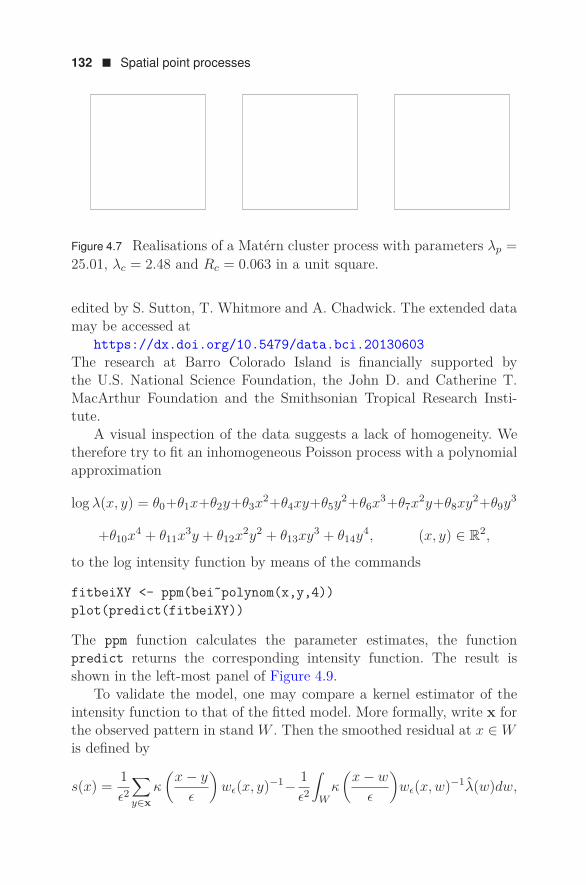
132 ! Spatial point processes
Figure 4.7 Realisations of a Matern cluster process with parameters λp =25.01, λc = 2.48 and Rc = 0.063 in a unit square.
edited by S. Sutton, T. Whitmore and A. Chadwick. The extended datamay be accessed at
https://dx.doi.org/10.5479/data.bci.20130603The research at Barro Colorado Island is financially supported bythe U.S. National Science Foundation, the John D. and Catherine T.MacArthur Foundation and the Smithsonian Tropical Research Insti-tute.
A visual inspection of the data suggests a lack of homogeneity. Wetherefore try to fit an inhomogeneous Poisson process with a polynomialapproximation
log λ(x, y) = θ0+θ1x+θ2y+θ3x2+θ4xy+θ5y2+θ6x3+θ7x2y+θ8xy2+θ9y3
+θ10x4 + θ11x3y + θ12x2y2 + θ13xy3 + θ14y4, (x, y) ∈ R2,
to the log intensity function by means of the commands
fitbeiXY <- ppm(bei˜polynom(x,y,4))plot(predict(fitbeiXY))
The ppm function calculates the parameter estimates, the functionpredict returns the corresponding intensity function. The result isshown in the left-most panel of Figure 4.9.
To validate the model, one may compare a kernel estimator of theintensity function to that of the fitted model. More formally, write x forthe observed pattern in stand W . Then the smoothed residual at x ∈ Wis defined by
s(x) = 1ϵ2
∑
y∈xκ
(x − y
ϵ
)wϵ(x, y)−1− 1
ϵ2
∫
Wκ
(x − w
ϵ
)wϵ(x, w)−1λ(w)dw,

Worked examples with R ! 133
Figure 4.8 The positions of Beilschmiedia trees in a 1,000 by 500 metrestand in Barro Colorado Island, Panama.
where κ is a symmetric probability density function and wϵ an edgecorrection factor. These residuals may be calculated using the functiondiagnose.ppm(fitbeiXY, which="smooth", sigma=100)and are plotted in the right-most panel of Figure 4.9.
Figure 4.9 Left: fitted intensity function λ(x, y) for Beilschmiedia trees inBarro Colorado Island using a fourth order polynomial approximationto the log intensity function. Right: smoothed residual surface using aGaussian kernel with σ = 100.
To test for homogeneity, apply the likelihood ratio test using thescripthombei <- ppm(bei˜1)anova(hombei, fitbeiXY, test = "LR")and find that the null hypothesis is emphatically rejected.
For further details, we refer to the vignettes of spatstat that areavailable on the CRAN websitehttps://cran.r-project.org.

134 ! Spatial point processes
4.13 EXERCISES
1. Let X1, X2, . . . be independent and exponentially distributed withparameter λ > 0 and define a point process on R+ by X =X1, X1 + X2, X1 + X2 + X3, . . . . Calculate P(NX((0, t]) = 0)for t ∈ R+.
2. Let X be a homogeneous Poisson process on the plane. Show thatthe squared distance from the origin to the nearest point of Xfollows an exponential distribution.
3. Let X be a Poisson process on Rd with intensity function λX , Y aPoisson process with intensity function λY . If X and Y are inde-pendent, show that the superposition X ∪ Y is a Poisson process.
4. Let X be a binomial point process of n ∈ N points on the unitsquare [0, 1]2. Calculate its factorial moment measures up to sec-ond order. Derive the covariance and pair correlation functions.Is X stationary and/or second order intensity-reweighted momentstationary?
5. Let W be a rectangle [a1, b1] × · · · × [ad, bd] ⊂ Rd for ai < bi ∈ R,i = 1, . . . , d. Give an explicit expression for the volume of W ∩ Wx
as a function of x ∈ Rd.
6. Let X be a point process on Rd for which product densities exist upto second order. In particular, assume that the first order momentmeasure exists and is absolutely continuous with density λ : Rd →R+. Denote by B(x, ϵ) the closed ball centred at x ∈ Rd withradius ϵ > 0 and write
"λ(x0) =∑
x∈X∩W
1x ∈ B(x0, ϵ)|B(x, ϵ) ∩ W | , x0 ∈ W,
for some open bounded Borel set W such that |W | > 0.
• Compute the expectation and variance of "λ(x0).• Suppose that n independent samples from the distribution of
X ∩ W are available. How would you estimate λ(x0)? Whatare the expectation and variance of your estimator?
7. Let X be a Poisson process on [0, 1]2 with intensity functionλ(x, y) = βeαy for α, β ≥ 0.

Exercises ! 135
• Estimate the parameters α and β based on an observed pat-tern x = (xi, yi) : i = 1, . . . , 10 for which ∑
i yi = 5.82.• Test the composite null hypothesis that X is homogeneous.
8. Is the Lennard–Jones interaction function of Example 4.11 locallystable? Is it hereditary?
9. For any finite point pattern x ⊂ W in the bounded Borel set W , let
Cx(w) =∑
x∈x1w ∈ B(x, R), w ∈ W,
be the coverage function of x. Here B(x, R) = w ∈ W : ||x −w|| ≤ R. Additionally, let V be a potential, that is, a functionV : N → R such that V (0) = 0. We would like to define a shotnoise-weighted point process X on W by means of an unnormaliseddensity of the form
f(x) ∝ exp[−
∫
WV (Cx(w))dw
]
with respect to the distribution of a unit rate Poisson processon W .
• Give a sufficient condition on the potential V for f to beintegrable.
• Show that X is a Markov point process with respect to therelation ∼ defined by x ∼ y if and only if ||x − y|| ≤ 2R,x, y ∈ W . Find an explicit expression for the clique interac-tion functions.Hint: Proceed as in the proof of the Hammersley–Cliffordtheorem.
10. Let X be a hard core process on some bounded Borel set W ⊂ Rd
with probability density
f(x = x1, . . . , xn) ∝ βn∏
u,v∈x1||u − v|| ≥ R
with respect to the distribution of a unit rate Poisson process.Estimate the interaction range R ≥ 0 and the parameter β ≥ 0.
11. Show that the pair correlation function of a planar Neyman–Scottprocess in which the daughters are located uniformly in a ball of

136 ! Spatial point processes
radius R > 0 around their parent depends only on the distance rbetween its arguments and is given by
g(r) = 1 + 4λpπ2rR
⎛
⎝ r
2Rarccos
(r
2R
)− r2
4R2
√
1 − r2
4R2
⎞
⎠
whenever 0 ≤ r ≤ 2R. This model is known as the Matern clusterprocess.Hint: use that the intersection area A(r, R) of two balls of radiusR whose centres are r apart is given by
A(r, R) = 2R2 arccos(r/(2R)) − r(4R2 − r2)1/2/2for r ∈ [0, 2R].
12. Let the random variable Λ be exponentially distributed with pa-rameter m > 0. Let X be a Cox process on Rd driven by Λ; that is,given Λ = λ, X is a homogeneous Poisson process with intensity λ.
• Give an explicit expression for the empty space function ofX in terms of the parameter m.
• How can you use your result to estimate m?
13. Let X be an inhomogeneous Poisson process on a bounded Borelset A ⊂ Rd defined by the intensity function λ : A → R+. As-sume that
∫A λ(a)da > 0. Prove that conditional on the number of
points, they are independent and identically distributed accordingto the probability density function
λ(a)∫A λ(a)da
on A. Compare the result to Theorem 4.2 and specialise to (4.11).
14. Let the random variable Λ be exponentially distributed with pa-rameter m > 0. Let Y be a Cox process on the bounded Borel setW ⊂ Rd driven by Λ; that is, given Λ = λ, Y is a homogeneousPoisson process on W with intensity λ. Compute the posteriordistribution of Λ given a realisation y of Y and its mean E [Λ | y].
15. The spatstat package contains a data set bei that contains treelocations in a tropical rain forest. Covariate information about thealtitude and slope in the study region is available in the accompa-nying data set bei.extra. Investigate whether altitude and slopeaffect the abundance of trees.

Pointers to the literature ! 137
4.14 POINTERS TO THE LITERATURE
It is difficult to point to the first documented use of the Poisson process.The name was probably coined in the late 1930s at the University ofStockholm and appears in the 1940 paper [1] by W. Feller who workedin Stockholm from 1934 until 1939. The phrase ‘point process’ is due toC. Palm [2]. This early work is mostly concerned with point processeson the real line. The foundations of a mathematically rigorous theory ofpoint processes on general state spaces were laid in the early 1960s byJ.E. Moyal [3] who used the now obsolete term ‘stochastic populationprocess’ in his title. We refer to a paper by Guttorp and Thorarinsdottir[4] for a more detailed historical overview and to the two volumes byDaley and Vere–Jones [5] for an exhaustive account of the theory ofpoint processes on Polish spaces.
The definition of a point process given in Section 4.1 can be found in[3]. In [6], A. Renyi proved that the void probabilities determine the dis-tribution of a Poisson process with diffuse intensity function, a result thatwas generalised to all simple point processes by G. Monch [7]. The basicfacts concerning a Poisson process are summarised in the monograph byJ.F.C. Kingman [8]. For example, his section 2.4 is devoted to a moregeneral version of Theorem 4.2. Perhaps confusingly, the name ‘Bernoulliprocess’ is used for the binomial point process, which is usually reservedfor sequences of binary valued random variables. Moment measures aredefined in Section 3 of [3]. Earlier work in the context of point processeson the real line includes that by A. Ramakrishnan [9], who advocatedthe use of product densities. The implications of various concepts ofstationarity, including homogeneity of the moments, are discussed ex-haustively in Chapter 12 of [5]. Definition 4.8 is adapted from a slightlymore general one due to Baddeley, Møller and Waagepetersen [10].
The consideration of stability can be traced back to L. Onsager [11]who called a probability density function f stable if the energy of a con-figuration x satisfies a linear lower bound in the number of points, thatis, − log(f(x)/f(∅)) ≥ −βn(x) for some β > 0. Additionally, Onsagershowed that the so-called hard core condition, which states that no twopoints can occur within a given positive distance of one another, im-plies stability. We refer to the textbook by D. Ruelle [12] for a rigoroustreatment of this and other notions of stability, their implications andmutual relations. The local stability condition, being defined in terms ofthe Papangelou conditional intensity [13], has become popular followingRipley and Kelly’s introduction of Markov point processes [14] specified

138 ! Spatial point processes
by their unnormalised densities. It implies the Onsager–Ruelle stabilitycondition. As an aside, unnormalised densities of the form exp(−|W |)fwith f given by (4.7) are known as Janossy densities to honour pioneeringwork [15]. The Strauss model was proposed in [16], the Lennard–Jonesinteraction function in [17]. Further examples of pairwise interactionmodels can be found in the textbooks [5] or [18].
Markov point processes were introduced in the statistical literatureby Ripley and Kelly [14], and our proof of Theorem 4.4 is taken from theirpaper. It should be noted, though, that the similar concept of a Gibbspoint process was already known in statistical physics; see for examplethe textbooks by C. Preston [19] and by D. Ruelle [12]. More recent de-velopments are reviewed in the monograph by M.N.M. van Lieshout [18].
Turning to statistics, the edge correction weight 1/|W ∩Wy−x|, com-monly known as the translation correction, in the kernel estimator (4.4)was proposed by Ohser and Stoyan [20]. For a fuller discussion of edgeeffects and ways to correct for them, we refer to Chapter 3 in the Adamsprize winning essay [21] by B.D. Ripley. Kernel estimators for the firstorder product density were introduced by P.J. Diggle [22], although witha focus on point processes on the real line. The mass-preserving kernelestimator (4.5) was suggested by M.N.M. van Lieshout [23].
Inference for Poisson processes based on their likelihood is treated ingreat detail in the book by Y.A. Kutoyants [24]. For non-Poisson models,the Monte Carlo maximum likelihood method of C.J. Geyer and E.A.Thompson [25] may be used. This method is generally applicable whenan unnormalised density function is explicitly available. The details forfinite point patterns are spelled out in [26], including Theorem 4.5 andthe Metropolis–Hastings sampler with birth and death proposals due toC.J. Geyer and J. Møller [27].
The idea to use maximum pseudo-likelihood for point processes canbe traced back to J.E. Besag, who, in [28], considered the special caseof the Strauss process. His approach is to approximate a spatial pointprocess by a series of random fields on finer and finer grids [29], withlabels in L = 0, 1 to denote presence or absence of points, and applypseudo-likelihood to the approximation. Our direct definition is takenfrom Jensen and Møller [30]. The method is implemented as the defaultparameter estimation technique in the R-package spatstat, the mostcomplete R-package devoted to spatial point pattern analysis [31]. Itserror estimates are based on a paper by Cœurjolly and Rubak [32]. Thesmoothed residuals implemented in the package are taken from an articleby Baddeley, Turner, Møller and Hazelton [33], which generalises earlier

References ! 139
ideas of Stoyan and Grabarnik [34]. Core functions are also implementedin the R-package spatial that comes with the default R implementationand in splancs.
A historical account on the introduction of Cox processes is givenby Guttorp and Thorarinsdottir [4]. They trace the Neyman–Scott clus-ter process to [35] and note that the special case where the daughtersare scattered according to a bivariate normal distribution (cf. Exam-ple 4.16) is called a modified Thomas process after work by M. Thomas[36] on a doubly stochastic model for the number of potato beetle lar-vae, even though their spatial location is not taken into account. TheMatern cluster process can be found in Section 3.6 of [37]. The productdensities up to second order were calculated by D. Vere–Jones [38] us-ing generating functional techniques. Although they are quite natural,log-Gaussian Cox processes seem to have been introduced as recently as1991 by Coles and Jones [39], who derived the pair correlation functionheuristically. The proof of Theorem 4.7 given here follows that in [40].Parameter estimation for such models by means of a minimum contrastmethod was proposed by P.J. Diggle [41]. The estimate of Rc in thecluster detection example of Section 4.11 is taken from this paper; thehierarchical analysis with a hard core prior follows Van Lieshout andBaddeley [42].
In closing, we recommend the textbooks by Møller and Waagepetersen[43], Illian, Penttinen, Stoyan and Stoyan [44] and Diggle [45] or part IVin [46] for further reading.
REFERENCES
[1] W. Feller (1940). On the integro-differential equations of purely discontinuousMarkoff processes. Transactions of the American Mathematical Society48(3):488–515.
[2] C. Palm (1943). Intensitatsschwenkungen im Fernsprechverkehr. EricssonTechnics, Volume 44.
[3] J.E. Moyal (1962). The general theory of stochastic population processes. ActaMathematica 108(1):1–31.
[4] P. Guttorp and T.L. Thorarinsdottir (2012). What happened to discrete chaos,the Quenouille process, and the sharp Markov property? Some historyof stochastic point processes. International Statistical Review 80(2):253–268.

140 ! Spatial point processes
[5] D.J. Daley and D. Vere-Jones (2003, 2008). An Introduction to the Theory ofPoint Processes (2nd edition). New York: Springer-Verlag.
[6] A. Renyi (1967). Remarks on the Poisson process. Studia Scientiarum Math-ematicarum Hungarica 2:119–123.
[7] G. Monch (1971). Verallgemeinerung eines Satzes von A. Renyi. Studia Scien-tiarum Mathematicarum Hungarica 6:81–90.
[8] J.F.C. Kingman (1993). Poisson Processes. Oxford: Clarendon Press.
[9] A. Ramakrishnan (1950). Stochastic processes relating to particles distributedin a continuous infinity of states. Proceedings of the Cambridge Philo-sophical Society 46(4):595–602.
[10] A.J. Baddeley, J. Møller and R. Waagepetersen (2000). Non- and semi-parametric estimation of interaction in inhomogeneous point patterns.Statistica Neerlandica 54(3):329–350.
[11] L. Onsager (1939). Electrostatic interaction of molecules. Journal of PhysicalChemistry 43(2):189–196.
[12] D. Ruelle (1969). Statistical Mechanics. Rigorous Results. New York: W.A.Benjamin.
[13] F. Papangelou (1974). The conditional intensity of general point processes andan application to line processes. Zeitschrift fur Wahrscheinlichkeitstheorieund verwandte Gebiete 28(3):207–226.
[14] B.D. Ripley and F.P. Kelly (1977). Markov point processes. Journal of theLondon Mathematical Society 15(1):188–192.
[15] L. Janossy (1950). On the absorption of a nucleon cascade. Proceedings of theRoyal Irish Academy 53(A):181–188.
[16] D.J. Strauss (1975). A model for clustering. Biometrika 62(2):467–475.
[17] J.E. Lennard–Jones (1924). On the determination of molecular fields. Proceed-ings of the Royal Society of London A106(838):441–477.
[18] M.N.M. van Lieshout (2000). Markov Point Processes and Their Applications.London: Imperial College Press.
[19] C. Preston (1976). Random Fields. Berlin: Springer-Verlag.
[20] J. Ohser and D. Stoyan (1981). On the second-order and orientation analysisof planar stationary point processes. Biometrical Journal 23(6):523–533.
[21] B.D. Ripley (1988). Statistical Inference for Spatial Processes. Cambridge:Cambridge University Press.

References ! 141
[22] P.J. Diggle (1985). A kernel method for smoothing point process data. AppliedStatistics 34(2):138–147.
[23] M.N.M. van Lieshout (2012). On estimation of the intensity function of a pointprocess. Methodology and Computing in Applied Probability 14(3):567–578.
[24] Y.A. Kutoyants (1998). Statistical Inference for Spatial Poisson Processes.New York: Springer-Verlag.
[25] C.J. Geyer and E.A. Thompson (1992). Constrained Monte Carlo maximumlikelihood for dependent data. Journal of the Royal Statistical SocietyB54(3):657–699.
[26] C.J. Geyer (1999). Likelihood inference for spatial point processes. In:Stochastic Geometry. Likelihood and Computation. Papers from the 3rdSeminaire Europeen de Statistique on Stochastic Geometry, Theory andApplications, Toulouse, 1996. Edited by O.E. Barndorff-Nielsen, W.S.Kendall and M.N.M. van Lieshout. Boca Raton, Florida: Chapman &Hall/CRC.
[27] C.J. Geyer and J. Møller (1994). Simulation procedures and likelihood in-ference for spatial point processes. Scandinavian Journal of Statistics21(4):359–373.
[28] J. Besag (1977). Some methods of statistical analysis for spatial data (withdiscussion). Proceedings of the 41st session of the ISI, New Delhi, 1977.Bulletin of the International Statistical Institute 47(2):77–91, 138–147.
[29] J. Besag, R. Milne and S. Zachary (1982). Point process limits of lattice pro-cesses. Journal of Applied Probability 19(1):210–216.
[30] J.L. Jensen and J. Møller (1991). Pseudolikelihood for exponential family mod-els of spatial point processes. The Annals of Applied Probability 1(3):445–461.
[31] A. Baddeley, E. Rubak and R. Turner (2015). Spatial Point Patterns:Methodology and Applications with R. Boca Raton, Florida: Chapman& Hall/CRC.
[32] J.-F. Cœurjolly and E. Rubak (2013). Fast covariance estimation for innova-tions computed from a spatial Gibbs point process. Scandinavian Journalof Statistics 40(4):669–684.
[33] A. Baddeley, R. Turner, J. Møller and M. Hazelton (2005). Residual anal-ysis for spatial point processes (with discussion). Journal of the RoyalStatistical Society B67(5):617–666.

142 ! Spatial point processes
[34] D. Stoyan and P. Grabarnik (1991). Second-order characteristics for stochas-tic structures connected with Gibbs point processes. MathematischeNachrichten 151(1):95–100.
[35] J. Neyman and E.L. Scott (1952). A theory of the spatial distribution of galax-ies. Astrophysical Journal 116:144–163.
[36] M. Thomas (1949). A generalization of Poisson’s binomial limit for use inecology. Biometrika 36(1/2):18–25.
[37] B. Matern (1986). Spatial Variation (2nd edition). Berlin: Springer-Verlag.
[38] D. Vere–Jones (1970). Stochastic models for earthquake occurrence. Journalof the Royal Statistical Society B32(1):1–62.
[39] P. Coles and B. Jones (1991). A lognormal model for the cosmological massdistribution. Monthly Notices of the Royal Astronomical Society 248(1):1–13.
[40] J. Møller, A.R. Syversveen and R.P. Waagepetersen (1998). Log Gaussian Coxprocesses. Scandinavian Journal of Statistics 25(3):451–482.
[41] P.J. Diggle (1978). On parameter estimation for spatial point processes. Jour-nal of the Royal Statistical Society B40(2):178–181.
[42] M.N.M. van Lieshout and A.J. Baddeley (2002). Extrapolating and interpolat-ing spatial patterns. In: Spatial Cluster Modelling. Edited by A.B. Lawsonand D.G.T. Denison. Boca Raton, Florida: Chapman & Hall/CRC.
[43] J. Møller and R.P. Waagepetersen (2004). Statistical Inference and Simulationfor Spatial Point Processes. Boca Raton, Florida: Chapman & Hall/CRC.
[44] J. Illian, A. Penttinen, H. Stoyan and D. Stoyan (2008). Statistical Analysisand Modelling of Spatial Point Patterns. Chichester: John Wiley & Sons.
[45] P.J. Diggle (2014). Statistical Analysis of Spatial and Spatio-Temporal PointPatterns (3rd edition). Boca Raton, Florida: Chapman & Hall/CRC.
[46] A.E. Gelfand, P.J. Diggle, M. Fuentes and P. Guttorp, editors (2010). Hand-book of Spatial Statistics. Boca Raton, Florida: Chapman & Hall/CRC.

Appendix: Solutions totheoretical exercises
EXERCISES IN CHAPTER 2
1. For k and m in N, without loss of generality suppose thatt1, . . . , tk ∈ A and tk+1, . . . , tk+m ∈ A. Pick x1, . . . , xk+m ∈ R.Then
Ft1,...,tk+m(x1, . . . , xk+m) = P(Z ≤ minx1, . . . , xk; 0≤ minxk+1, . . . , xk+m),
which in terms of the cumulative distribution function FZ of Zreads
FZ(minx1, . . . , xk)if 0 ≤ minxk+1, . . . , xk+m and zero otherwise. If m = 0 andk ∈ N, then Ft1,...,tk(x1, . . . , xk) = FZ(minx1, . . . , xk). Finally, ifk = 0 and m ∈ N, then
Ft1,...,tm(x1, . . . , xm) =
1 if 0 ≤ minx1, . . . , xm;0 otherwise.
2. SinceCov(Xs, Xt) =
n∑
i=1
n∑
j=1Cov(Zifi(s), Zjfj(t)),
the covariance function ρ of X is given by
ρ(s, t) =n∑
i=1
n∑
j=1fi(s)fj(t)Cov(Zi, Zj).
143

144 ! Appendix: Solutions to theoretical exercises
3. First, note that mY (t) = EYt = EX2t = ρ(t, t) + m(t)2. Moreover
ρY (s, t) = E(X2s X2
t ) − mY (s)mY (t).
It remains to calculate E(X2s X2
t ). Now,
E(X2s X2
t ) = E[(Xs − m(s) + m(s))2(Xt − m(t) + m(t))2
]
= E[(Xs − m(s))2(Xt − m(t))2
]
+ E[(Xs − m(s))2m(t)2 + (Xt − m(t))2m(s)2
]
+ E [4m(s)m(t)(Xs − m(s))(Xt − m(t))] + m(s)2m(t)2
since the odd central moments of a multivariate normal distribu-tion are zero. Hence
E(X2s X2
t ) = E[(Xs − m(s))2(Xt − m(t))2
]+ m(t)2ρ(s, s)
+ m(s)2ρ(t, t) + m(s)2m(t)2 + 4m(s)m(t)ρ(s, t).
By the hint, if Z = (Zs, Zt) is bivariate normally distributed withmean zero,
E(Z2s Z2
t ) = ρZ(s, s)ρZ(t, t) + 2ρZ(s, t)2,
where ρZ is the covariance function of Z, so
E(X2s X2
t ) = ρ(s, s)ρ(t, t) + 2ρ(s, t)2 + m(t)2ρ(s, s)+ m(s)2ρ(t, t) + m(s)2m(t)2 + 4m(s)m(t)ρ(s, t)
= ρ(s, s)mY (t) + m(s)2mY (t) + 2ρ(s, t)2
+ 4m(s)m(t)ρ(s, t)= mY (s)mY (t) + 2ρ(s, t)2 + 4m(s)m(t)ρ(s, t).
In conclusion,
ρY (s, t) = E(X2s X2
t ) − mY (s)mY (t) = 2ρ(s, t)2 + 4m(s)m(t)ρ(s, t).
4. Regarding the first claim note that, for a1, . . . , an ∈ R, n ∈ N, thedouble sum
n∑
i=1
n∑
i=1aiaj (αρ1(ti, tj) + βρ2(ti, tj))
= αn∑
i=1
n∑
j=1aiajρ1(ti, tj) + β
n∑
i=1
n∑
j=1aiajρ2(ti, tj)

Exercises in Chapter 2 ! 145
is non-negative when α and β are non-negative.To prove the second claim, let X and Y be independent zero meanGaussian random fields with covariance functions ρ1 and ρ2 re-spectively (cf. Proposition 2.1). Then the covariance function ofthe random field Z defined by Zt = XtYt, t ∈ Rd, is equal to
Cov(Z(t1), Z(t2)) = E [X(t1)Y (t1)X(t2)Y (t2)] = ρ1(t1, t2)ρ2(t1, t2)
by the assumed independence. In other words, the product ρ1ρ2 isthe covariance function of Z and therefore non-negative definite.
5. For n ∈ N and 0 < t1 < · · · < tn, consider the n × n matrix Σn
with entries ρ(ti, tj), i, j ∈ 1, . . . , n:
Σn =
⎛
⎜⎜⎜⎜⎜⎝
t1 t1 · · · t1 t1t1 t2 · · · t2 t2
· · · · · · · · · · · · · · ·t1 t2 · · · tn−1 tn−1t1 t2 · · · tn−1 tn
⎞
⎟⎟⎟⎟⎟⎠.
We proceed to show that Σn is non-negative definite. Using theSylvester criterion, we shall show that the determinants of allupper-left sub-blocks are positive. Note that they take the sameshape as the matrix Σn itself. Equivalently therefore, it suffices toshow that the determinant of Σn is positive for all n ∈ N.For n = 1, the matrix (t1) has determinant t1 > 0. For n = 2, thematrix (
t1 t1t1 t2
)
has determinant t1(t2 − t1) > 0. We claim that the determinant ofΣn is t1(t2 − t1) · · · (tn − tn−1) > 0 by the chronological ordering.The claim may be proven by induction and the fact that
detΣn = det
⎛
⎜⎜⎜⎜⎜⎝
t1 t1 · · · t1 t10 t2 − t1 · · · t2 − t1 t2 − t10 · · · · · · · · · · · ·0 t2 − t1 · · · tn−1 − t1 tn−1 − t10 t2 − t1 · · · tn−1 − t1 tn − t1
⎞
⎟⎟⎟⎟⎟⎠
= t1det
⎛
⎜⎜⎜⎝
t2 − t1 · · · t2 − t1 t2 − t1· · · · · · · · · · · ·
t2 − t1 · · · tn−1 − t1 tn−1 − t1t2 − t1 · · · tn−1 − t1 tn − t1
⎞
⎟⎟⎟⎠ ,

146 ! Appendix: Solutions to theoretical exercises
which has the same form as Σn−1.
6. By Bochner’s theorem, the spectral density reads, for w ∈ R,
f(w) = 12π
∫ ∞
−∞
12β
e−β|t|e−iwtdt.
Split f(w) in integrals over R+ and R−. Then, noting that thefunction t → et is a primitive of itself,
∫ ∞
0e−β|t|e−iwtdt = 1
β + iw= 1
β + iw
β − iw
β − iw= β − iw
β2 + w2 .
Similarly,∫ 0
−∞e−β|t|e−iwtdt = 1
β − iw= β + iw
β2 + w2 .
Hence
f(w) = 14πβ
1β2 + w2 (β − iw + β + iw) = 1
2π
1β2 + w2 , w ∈ R.
To verify the existence of a continuous version, note that the inte-gral ∫ ∞
−∞|w|ϵf(w)dw = 1
2π
∫ ∞
−∞
|w|ϵ
β2 + w2 dw
is finite for ϵ < 1.
7. First, let us calculate the Fourier transform of the box function φ.Now,
∫
Rφ(s)e−iξsds =
∫ 1/2
−1/2e−iξsds = e−iξ/2 − eiξ/2
−iξ= sin(ξ/2)
ξ/2 .
The convolution of φ with itself is, for t ∈ R, given by
φ ∗ φ(t) =∫ ∞
−∞φ(s)φ(t − s)ds =
∫ 1/2
−1/21
t − 1
2 ≤ s ≤ t + 12
ds,
the length of the intersection[−1
2 ,12
]∩
[t − 1
2 , t + 12
].
The intersection length is equal to min(1/2, t+1/2)−max(−1/2, t−1/2) provided that the intersection is not empty. Hence, for |t| ≤ 1,φ ∗ φ(t) = θ(t). Recalling that the Fourier transform of a convo-lution is the product of the Fourier transforms, one obtains thedesired result for the function θ.

Exercises in Chapter 2 ! 147
8. Note thatρ(θ) =
∞∑
j=0σ2
j
[eijθ + e−ijθ
2
]
is in the spectral form of Bochner’s theorem with µ(j) = σ2j /2 for
j ∈ Z. Clearly µ is non-negative and symmetric. It takes finitevalues whenever ∞∑
j=0σ2
j < ∞.
The cosine is uniformly continuous on its compact domain, so ρ iscontinuous as a limit of uniformly continuous functions.Continuous versions exist if
∞∑
j=0jϵσ2
j < ∞
for some ϵ ∈ (0, 1). Plug in σ2j = (α+βj2p)−1. Then for 2p − ϵ > 1,
that is, for p > 1/2, ρ is well-defined and the corresponding Gaus-sian field admits a continuous version.
9. The sill islim
|t|→∞γ(t) = α + β,
the nuggetlim
|t|→0γ(t) = α.
The partial sill is the difference between the two limits, β.
10. By Theorem 2.2, the general expression is
Xt0 = 1σ2
[ρ(t0, t1) ρ(t0, t2)
] [1 ρρ 1
]−1 [Xt1
Xt2
]
= 1σ2
11 − ρ2
[ρ(t0, t1) ρ(t0, t2)
] [1 −ρ
−ρ 1
] [Xt1
Xt2
]
= 1σ2
11 − ρ2 (ρ(t0, t1) − ρρ(t0, t2))Xt1 + (ρ(t0, t2) − ρρ(t0, t1))Xt2.
For the special cases one obtains the following expressions:
• 1σ2
11−ρ2 ρ(t0, t1)Xt1 − ρρ(t0, t1)Xt2, which does depend
on Xt2 ;

148 ! Appendix: Solutions to theoretical exercises
• 0 as Xt1 and Xt2 do not provide any information;• 1
σ2 ρ(t0, t1)Xt1 + ρ(t0, t2)Xt2 .
The mean squared prediction error is
ρ(t0, t0) − 1σ2
11 − ρ2
[ρ(t0, t1) ρ(t0, t2)
] [1 −ρ
−ρ 1
] [ρ(t0, t1)ρ(t0, t2)
]
= ρ(t0, t0) − 1σ2
11 − ρ2
ρ(t0, t1)2 + ρ(t0, t2)2 − 2ρρ(t0, t1)ρ(t0, t2)
.
For the special cases one gets the following:
• ρ(t0, t0) − 1σ2
ρ(t0,t1)2
1−ρ2 ;• ρ(t0, t0);• ρ(t0, t0) − 1
σ2ρ(t0, t1)2 + ρ(t0, t2)2
.
11. Assume that the covariance structure of (Et)t∈Rd is known as wellas β and m. Write Σ for the covariance matrix of Eti , i = 1, . . . , n,and K for the n × 1 vector with entries Cov(Et0 , Eti). Then
Xt0 = m(t0)′β + K ′Σ−1(Xti − m(ti)′β)n×1
according to Theorem 2.2.If β were unknown one might try to estimate it, for instance bythe maximum likelihood method. The log likelihood of the obser-vations is proportional to
−(Xti − m(ti)′β)1×nΣ−1(Xti − m(ti)′β)n×1,
so the score equations are
2M ′Σ−1(Xti − m(ti)′β)n×1 = 0,
where M is the n × p matrix whose rows are the m(ti)′. Hence,provided that the matrix M ′Σ−1M is invertible,
β = (M ′Σ−1M)−1M ′Σ−1Z,
writing Z for the n × 1 vector of observations Xti . Finally, plug βinto the expression for the kriging estimator.

Exercises in Chapter 2 ! 149
12. First compute
m =
1σ2(1−ρ2)
[1 1
] [1 −ρ
−ρ 1
] [Xt1
Xt2
]
1σ2(1−ρ2)
[1 1
] [1 −ρ
−ρ 1
] [11
] = Xt1 + Xt2
2 ,
the mean. Then plug m into the simple kriging estimator (cf. Ex-ercise 10) to obtain
Xt0 = m + 1σ2
11 − ρ2 (ρ(t0, t1) − ρρ(t0, t2))(Xt1 − m)
+ 1σ2
11 − ρ2 (ρ(t0, t2) − ρρ(t0, t1))(Xt2 − m)
= Xt1 + Xt2
2 + 12σ2
11 − ρ2 (ρ(t0, t1) − ρρ(t0, t2))(Xt1 − Xt2)
+ 12σ2
11 − ρ2 (ρ(t0, t2) − ρρ(t0, t1))(Xt2 − Xt1)
= Xt1 + Xt2
2 + (ρ(t0, t1) − ρ(t0, t2))(Xt1 − Xt2)2σ2(1 − ρ) .
When ρ(t0, t2) = 0, Xt0 is given byXt1 + Xt2
2 + ρ(t0, t1)(Xt1 − Xt2)2σ2(1 − ρ) .
If additionally ρ(t0, t1) = 0 then
Xt0 = Xt1 + Xt2
2 ,
the mean of Xt1 and Xt2 . In both cases the expression for Xt0
involves both Xt1 and Xt2 .If ρ = 0,
Xt0 = Xt1 + Xt2
2 + (ρ(t0, t1) − ρ(t0, t2))(Xt1 − Xt2)2σ2 .
The mean squared prediction error exceeds that of simple krigingby a term
(1 − 1′Σ−1K)2
1′Σ−11 =(σ2(1 + ρ) − ρ(t0, t1) − ρ(t0, t2)
)2
2σ2(1 + ρ)according to Theorem 2.4.

150 ! Appendix: Solutions to theoretical exercises
13. Since the null-space is non-trivial, one can find an n-vector a suchthat Σa = 0 and Var(a′Z) = a′Σa = 0. Then Cov(c′Z, a′Z) =c′Σa = 0 for all vectors c. Also 0 = Cov(Xt0 , a′Z) = K ′a. We haveshown that K is orthogonal to the null space of Σ. Therefore, bythe symmetry of Σ, K lies in its column space.
14. Write(
n∑
i=1ciXti − Xt0
)2
=(
n∑
i=1ci(Xti − m(ti)′β) − (Xt0 − m(t0)′β)
+
n∑
i=1cim(ti)′ − m(t0)′
β
)2
.
The last term is zero under the constraint and may be omitted.Consequently the mean squared error is equal to
EE2t0 +E
(n∑
i=1ciEti
)2
−2E(
Et0
n∑
i=1ciEti
)
= ρ(t0, t0)+c′Σc−2c′K.
The p-dimensional Euler–Lagrange multiplier λ ∈ Rp adds a term
λ′(
n∑
i=1cim(ti) − m(t0)
)
= λ′(M ′c − m(t0)).
Hence, the score equations are
2Σc − 2K + Mλ = 0
andM ′c = m(t0).
Pre-multiplication of the first score equation by M ′Σ−1 and thefact that M ′c = m(t0) yield λ = 2(M ′Σ−1M)−1(M ′Σ−1K −m(t0))and consequently
Σc = K − M(M ′Σ−1M)−1(M ′Σ−1K − m(t0)),
from which the desired result follows.

Exercises in Chapter 3 ! 151
EXERCISES IN CHAPTER 3
1. Suppose that (xj)j =i is feasible in the sense that xjxk = 0 wheneverj ∼ k. Then
πi(1 | xj , j = i)πi(0 | xj , j = i) =
a if xj = 0 for j ∼ i0 otherwise
depends on the neighbours of i only, so X is Markov with respectto ∼. Furthermore, if xj = 0 for all j ∼ i then πi(1 | xj , j = i) =1 − πi(0 | xj , j = i) = a/(1 + a). If xj = 1 for some j ∼ i thenπi(0 | xj , j = i) = 1.Consider a lattice that consists of two adjacent sites labelled 1 and2 and take y = (0, 1), x = (1, 0). Then both x and y have positiveprobability of occurring, but π2(y2 | x1) = π2(1 | 1) = 0.
2. Without loss of generality, consider the first two elements of X.If the joint covariance matrix is Σ = (I − B)−1K, we know thatthe conditional covariance matrix of the first block consisting ofX1 and X2 is Σ11 − Σ12Σ−1
22 Σ21. To find an explicit expression, usethe hint applied to I − B. Thus, A12 = −B12, A21 = −B21 andA22 = I − B22. Partition the matrix K in four blocks too, sayK1, K2 on the diagonal, 0 off the diagonal.Now,
(A−1)11 = I + B12(I − B22 − B21B12)−1B21,
(A−1)12 = B12(I − B22 − B21B12)−1,
(A−1)21 = (I − B22 − B21B12)−1B21,
(A−1)22 = (I − B22 − B21B12)−1.
Hence the conditional covariance matrix Σ11 − Σ12Σ−122 Σ21 reads
(A−1)11K1 − (A−1)12K2(K2)−1((A−1)22)−1(A−1)21K1
= K1 + B12(I − B22 − B21B12)−1B21K1 − B12(I − B22
− B21B12)−1B21K1 = K1.
Since K1 is diagonal, X1 and X2 are uncorrelated and therefore,being normally distributed, independent.

152 ! Appendix: Solutions to theoretical exercises
Unconditionally, the covariance between X1 and X2 is Σ11 =(A−1)11K1, that is,
(I − B12(I − B22)−1B21)−1[
κ1 00 κ2
]
.
Here we use the simplification (A−1)11 = (I − B12(I − B22)−1
B21)−1. As this matrix is not necessarily diagonal, X1 and X2 maybe dependent.
3. The local characteristics are well-defined normal densities. UsingBesag’s factorisation theorem, the joint density would be propor-tional to
π1(x | 0)π2(y | x)π1(0 | 0)π2(0 | x) = exp
[−1
2(y − x)2]
, (x, y) ∈ R2.
However, this function is not integrable.
4. Since πi(0 | yT \i) = e−µi , respectively πi(l | yT \i) = e−µiµli/l! for
l ∈ N, by the factorisation theorem,
πY (y)πY (0) = exp
⎡
⎣θ∑
i∼j;i<j
yiyj −∑
i∈T
log yi!
⎤
⎦ .
Now θ∑
i∼j;i<j yiyj ≤ 0 for θ ≤ 0 and therefore
∑
y∈(N0)T
πY (y)πY (0) ≤
∑
y∈(N0)T
exp[
−∑
i∈T
log yi!]
=( ∞∑
l=0
1l!
)|T |
< ∞.
For θ > 0, without loss of generality consider the first two sitesand suppose that 1 ∼ 2. Then
πY (y1, y2, 0, . . . , 0)πY (0) = eθy1y2
y1!y2!
should be summable. However, the series∞∑
y1=0
∞∑
y2=0
eθy1y2
y1!y2!
diverges as the general term does not go to zero.

Exercises in Chapter 3 ! 153
5. The first task is to find the maximum likelihood estimator for µ.Assume that B is a symmetric matrix with zeroes on the diago-nal such that I − B is positive definite. Then the log likelihoodL(µ; X) is
−12(X − µ1)′(I − B)(X − µ1).
The score equations is given by
0 = 1′(I − B)(X − µ1).
Therefore
µ = 1′(I − B)X1′(I − B)1 =
∑t∈T Xt(1 −
∑s∈T bst)
|T | −∑
s∈T
∑t∈T bst
is a linear function of X, hence normally distributed with mean µand variance (1′(I −B)1)−1, that is, 1/(|T |−
∑s∈T
∑t∈T bst). The
variance does not depend on µ. A two-sided test rejects if
|µ| >ξ1−α/2
(|T | −∑
s∈T
∑t∈T bst)1/2
or, equivalently, if∣∣∣∣∣∑
t∈T
Xt(1 −∑
s∈T
bst)∣∣∣∣∣ >
(
|T | −∑
s∈T
∑
t∈T
bst
)1/2
ξ1−α/2.
Here ξ1−α/2 is the 1 − α/2 quantile of the standard normal distri-bution and α ∈ (0, 1) the desired level of the test.An alternative would be to use the likelihood ratio test statistic
Λ(X) = exp [L(0; X) − L(µ; X)] = exp[1
2 µ21′(I − B)1 − µ1′(I − B)X]
= exp[− (1′(I − B)X)2
2(1′(I − B)1
].
The likelihood ratio test rejects the null hypothesis for large val-ues of
−2 log Λ(X) = (1′(I − B)X)2
1′(I − B)1 = (µ)2
Var(µ) .
Under the null hypothesis, −2 log Λ(X), as the square of a stan-dard normally distributed random variable, is χ2-distributed withone degree of freedom. It is interesting to observe that the twoapproaches lead to the same test!

154 ! Appendix: Solutions to theoretical exercises
6. A potential V is normalised with respect to 0 if VA(x) = 0 when-ever xi = 0 for some i ∈ A. This is clearly the case for sets A ofcardinality one or two. For larger A, VA(x) = 0 too.
7. By definition, V∅ = 0. For A = i, by Theorem 3.2,
Vi(y) = − log πi(0 | 0, . . . , 0) + log πi(yi | 0, . . . , 0) = − log yi!
and for A = i, j, again by Theorem 3.2, Vi,j(y) is equal to
log πi(0 | 0, . . . , 0) − log πi(yi | 0, . . . , 0)
− log πi(0 | yj , 0, . . . , 0) + log πi(yi | yj , 0, . . . , 0),so
Vi,j(y) = −yiyj1i ∼ j.
Since the joint distribution is proportional to
exp
⎡
⎣−∑
i∼j;i<j
yiyj −∑
i∈T
log yi!
⎤
⎦
(cf. Exercise 4), all other potentials vanish.
8. Write x for the realisation on the set A of crossed sites, y for that ondotted sites. Then, reasoning as in the proof of the spatial Markovproperty,
πA(x | y) ∝∏
A∩C =∅ϕC(xA∩C , yC\A),
where C runs through the family of cliques with respect to ∼. Now,the cliques with respect to ∼ are the empty set, singletons andpairs of horizontally or vertically adjacent sites. The latter alwayscombine a crossed and dotted site. Hence the factorisation doesnot contain terms with two different xis and the proof is complete.
9. As mentioned in Example 3.4, the local characteristics at i ∈ Tare normally distributed with variance κi and mean
∑
j =i
bijxj =∑
j∼i
bijxj .
Therefore, the local characteristic at i depends on xT \i onlythrough xj at sites j that are neighbours of i. Hence the CAR
Exercises in Chapter 3 ! 155
model is a Markov random field. Its joint probability density func-tion satisfies
log π(x) ∝ −12x′K−1(I − B)x = −1
2∑
i∈T
x2i
κi+ 1
2∑
i∈T
∑
j∈T
bijxixj
κi.
Hence ϕ(xi) = exp(−x2i /(2κi)) and
ϕ(xi, xj) = exp(bijxixj/(2κi)) = exp(bjixixj/(2κj)),
recalling that K−1(I −B) is symmetric by definition. If i ∼ j, thenbij = 0 and consequently ϕ(xi, xj) = 1.
10. The proposal mechanism in a Metropolis–Hastings sampler couldbe to select a site uniformly at random. If site i is selected, a newlabel could be chosen according to πi(· | xj , j = i).To prove convergence, observe that the chain restricted to feasi-ble states is aperiodic due to self-transitions. It is also irreducible,since to get from feasible state x to feasible state y, one may changeall 1s in x to 0 first, then change those sites with label 1 in y to 1.By Proposition 3.2, πX defines an invariant probability measure.An appeal to the fundamental convergence theorem completes theproof.To find a Monte Carlo maximum likelihood estimator for a, con-sider the ratio πX(x; a)/πX(x; a0), for example with respect to thereference parameter a0 = 1, and note that the ratio of normalisingconstants can be written as an expectation. Finally, approximatethe expectation by an average over a sample from πX(·; a0) ob-tained by the method just described.
11. The maximum likelihood estimators that optimise
L(β, σ2; Y ) = − 12σ2 (Y − Xβ)′(I − B)(Y − Xβ) − n log σ
are
β = (X ′(I − B)X)−1X ′(I − B)Y
σ2 = 1n
(Y − Xβ)′(I − B)(Y − Xβ).
To see this, proceed as in Section 3.5 for the SAR model with(I − B′)(I − B) replaced by I − B.

156 ! Appendix: Solutions to theoretical exercises
Regarding maximum pseudo-likelihood estimation, the local char-acteristics are Gaussians with mean
E(Yi|YT \i) = (Xβ)i +∑
j =i
bij(Yj − (Xβ)j), i ∈ T,
and variance σ2. Therefore
PL(β, σ2; Y ) = −∑
i∈T
12σ2
⎛
⎝Yi − (Xβ)i −∑
j =i
bij(Yj − (Xβ)j)
⎞
⎠2
− n log σ
= − 12σ2 (Y − Xβ)′(I − B)2(Y − Xβ) − n log σ.
Note that PL(β, σ2; Y ) is equal to the log likelihood of the SARmodel. Hence the maximum pseudo-likelihood estimators β and σ2
are given by
β = (X ′(I − B)2X)−1X ′(I − B)2Y
σ2 = 1n
(Y − Xβ)′(I − B)2(Y − Xβ).
12. Write Sil (x) for S evaluated at the configuration y that takes the
value l at site i and is equal to x at all other sites. Then the localcharacteristics can be written as
πi(xi | xT \i) = exp(θS(x))∑
l∈0,1 exp(θSi
l (x)) , i ∈ T, x ∈ 0, 1T .
Therefore,
log πi(xi | xT \i) = θS(x) − log
⎛
⎝∑
l∈0,1exp(θSi
l (x))
⎞
⎠ .
Take the derivative with respect to the parameter θ to obtain
S(x) − 1∑
l∈0,1 exp(θSil (x))
∑
l∈0,1Si
l (x) exp(θSil (x)).
The second term is equal to Eθ
[S(X) | XT \i = xT \i
]. To complete
the proof, sum over all sites and equate the pseudo-likelihood scoreequation thus obtained to zero.

Exercises in Chapter 3 ! 157
13. We claim thatπX(x)q(x, y) = πX(y)q(y, x)
for all x, y ∈ LT . To see this, note that q(x, y) = 0 = q(y, x) ifx and y differ in two or more sites. For such x and y the claimobviously holds as it does for y = x.Thus, assume that x and y differ in exactly one site, say i ∈ T .Then,
πX(x)q(x, y) = πX(x) 1|T |πi(yi | xT \i)
= πi(xi | xT \i)P(XT \i = xT \i)1
|T |πi(yi | xT \i)
= πi(xi | xT \i)1
|T |πX(y) = q(y, x)πX(y).
It follows that A(x, y) = 1 and the detailed balance equationscoincide with the claim.
14. The greedy algorithm optimises, iteratively over i ∈ T ,
−12σ2 (yi − l)2 + θ
∑
j∼i
1xj = l
as a function of l ∈ L. For θ = 0, the optimal l is that label in Lthat is closest to yi. For θ → ∞, l is chosen by a majority voteunder the labels of sites that are neighbours of i.

158 ! Appendix: Solutions to theoretical exercises
EXERCISES IN CHAPTER 4
1. For k = 0, 1, . . . ,
P(NX((0, t]) = k) = P(X1 + · · · + Xk ≤ t; X1 + · · · + Xk+1 > t)
=∫ t
0
λkrk−1
(k − 1)!e−λre−λ(t−r)dr = e−λt (λt)k
k!
using the fact that the sum X1 + · · · + Xk is Erlang distributed.Therefore NX((0, t]) is Poisson distributed with parameter λt. Plugin k = 0 to see that the void probability of (0, t] is equal toexp(−λt).
2. The cumulative distribution function of the squared distanced(0, X)2 of X to the origin can be written in terms of a void prob-ability. Indeed,
P(d(0, X)2 ≤ r) = 1−P(d(0, X)2 > r) = 1−P(X ∩B(0,√
r) = ∅),
where B(0,√
r) is the closed ball centred at 0 with radius √r.
Since 1 − v(B(0,√
r)) = 1 − exp(−λπr), d(0, X)2 is exponentiallydistributed.
3. Observe that for any bounded Borel set A ⊂ Rd,
P((X ∪ Y ) ∩ A = ∅) = P(X ∩ A = ∅; Y ∩ A = ∅)= P(X ∩ A = ∅)P(Y ∩ A = ∅)
by the independence of X and Y . Since X and Y are Poissonprocesses, the product of the two void probabilities is
exp[−
∫
AλX(z)dz
]exp
[−
∫
AλY (z)dz
]
= exp[−
∫
A(λX(z) + λY (z))dz
],
the void probability v(A) of a Poisson process with intensity func-tion λX + λY . An appeal to Theorem 4.1 completes the proof.
4. For a Borel set A ⊆ [0, 1]2,
α(1)(A) = nP(X1 ∈ A) = n|A|

Exercises in Chapter 4 ! 159
is absolutely continuous with product density ρ(1)(x) = n for allx ∈ [0, 1]2. Similarly, for two Borel sets A, B ⊆ [0, 1]2,
α(2)(A × B) = E
⎡
⎣n∑
i=1
∑
j =i
1Xi ∈ A; Xj ∈ B
⎤
⎦
= n(n − 1)|A||B|
since Xi and Xj are independent when i = j. Moreover, α(2) is ab-solutely continuous with second order product density ρ(2)(x, y) =n(n − 1) on [0, 1]2. Turning to derived statistics, the second ordermoment measure is
µ(2)(A×B) = α(2)(A×B)+α(1)(A∩B) = n(n−1)|A||B|+n|A∩B|,
the covariance reads
µ(2)(A × B) − α(1)(A)α(1)(B) = n|A ∩ B| − n|A||B|
and the pair correlation function is
g(x, y) = ρ(2)(x, y)ρ(1)(x)ρ(1)(y) = 1 − 1
n, x, y ∈ [0, 1]2.
Since the point process is defined on the unit square only, it cannotbe stationary. The pair correlation function and first order productdensity are constant. The latter is also strictly positive, so X issecond order intensity-reweighted moment stationary.
5. First consider the one-dimensional case. For x > 0,
[a, b] ∩ [a + x, b + x] = [a + x, b]
if x ≤ b − a and empty otherwise. Similarly for x < 0,
[a, b] ∩ [a + x, b + x] = [a, b + x]
provided −x ≤ b − a. In both cases, the length is b − a − |x| if|x| < b − a and zero otherwise. Repeating these arguments for allcomponents in d dimensions, one obtains
|W ∩ Wx| =d∏
i=1(bi − ai − |xi|)+.

160 ! Appendix: Solutions to theoretical exercises
6. By (4.2), the first two moments are given by
E["λ(x0)
]=
∫
B(x0,ϵ)∩W
λ(x)|B(x, ϵ) ∩ W |dx
and
E[(
!λ(x0))2]
= E
⎡
⎣∑ =
(x,y)∈(X∩W )2
1x ∈ B(x0, ϵ)|B(x, ϵ) ∩ W |
1y ∈ B(x0, ϵ)|B(y, ϵ) ∩ W |
⎤
⎦
+ E[
∑
x∈X∩W
1x ∈ B(x0, ϵ)|B(x, ϵ) ∩ W |2
]
=∫
B(x0,ϵ)∩W
∫
B(x0,ϵ)∩W
ρ(2)(x, y)|B(x, ϵ) ∩ W ||B(y, ϵ) ∩ W |dxdy
+∫
B(x0,ϵ)∩W
λ(x)|B(x, ϵ) ∩ W |2 dx.
Provided λ(·) > 0, the variance is∫
B(x0,ϵ)∩W
∫
B(x0,ϵ)∩W
(g(x, y) − 1)λ(x)λ(y)|B(x, ϵ) ∩ W ||B(y, ϵ) ∩ W |dxdy
+∫
B(x0,ϵ)∩W
λ(x)|B(x, ϵ) ∩ W |2 dx.
If there is replication, write Ti(Xi) for the estimator "λ(x0) appliedto Xi. The combined estimator is then the average ∑n
i=1 Ti(Xi)/n.The expectation is not altered by replication. The variance howeveris much reduced, by a factor 1/n. (Also the problem of distinguish-ing between inhomogeneity and clustering disappears).
7. The log likelihood function based on x = (x1, y1), . . . , (xn, yn) isgiven by
n log β + αn∑
i=1yi − β
∫ 1
0eαydy.
The score equations read
0 = n
β−
∫ 1
0eαydy = 10
β−
∫ 1
0eαydy;
0 =n∑
i=1yi − β
∫ 1
0yeαydy = 5.82 − β
∫ 1
0yeαydy.

Exercises in Chapter 4 ! 161
Numerical optimisation yields α = 1.00, β = 5.82. The determi-nant
n
β
∫ 1
0y2eαydy −
(∫ 1
0yeαydy
)2
of the Hessian matrix H(α, β) is positive. Since the principal minor−n/(β2) is negative, (α, β) maximises the log likelihood function.To test the null hypothesis that α = 0, use the likelihood ratiotest. Under the null hypothesis, the maximum likelihood estimatoris β0 = 10. Therefore, the likelihood ratio test statistic is
Λ(x) = f(x; 0, β0)f(x; α, β)
=(β0)n exp
[−β0
]
(β)n exp[α
∑ni=1 yi − β
∫ 10 eαydy
]
≈ exp(−0.41)
and −2 log Λ(X) ≈ 0.81 should be compared to an appropriatequantile of a χ2 distribution with one degree of freedom.
8. The interaction function is strictly positive and hence hereditary. Itis not locally stable. To see this, note that γ(u, v) is strictly largerthan one if ||u − v|| > (β/α)1/6 and has an asymptote at one for||u − v|| → ∞. The continuity of the interaction function impliesthat there exists a constant γ > 1 such that γ(u, v) > γ if ||u − v||lies in an appropriately chosen interval [r1, r2], (β/α)1/6 < r1 <r2 < ∞. Consequently the conditional intensity λ(u|x) is largerthan γn for point patterns x containing n points xi ∈ x such that||u − xi|| ∈ [r1, r2]. Since γn → ∞ as n → ∞, the conditionalintensity cannot be bounded.
9. A sufficient condition for integrability is that there exists someβ > 0 such that
|V (n)| ≤ βn for all n ∈ N0.
Use induction with respect to the number of points as in the proofof the Hammersley–Clifford theorem to show that for x = ∅ theinteraction functions satisfy
ϕ(x) = exp
⎡
⎣−∫
W
∑
y⊆x(−1)n(x\y)V (Cy(w))dw
⎤
⎦

162 ! Appendix: Solutions to theoretical exercises
= exp
⎡
⎣−|⋂
x∈xB(x, R)|
n(x)∑
i=1
(n(x)
i
)
(−1)n(x)−iV (i)
⎤
⎦ ,
using the notation n(x) for the cardinality of x.The first equation in the claim clearly holds when x is a singleton.Assume that ϕ has this form for configurations with up to n ≥ 1points and let x be such that n(x) = n. Then, for u ∈ x,
ϕ(x ∪ u) = f(x ∪ u)∏
x∪u =y⊂x∪u ϕ(y)
= exp[−
∫
W
V (Cx∪u(w))
−∑
x∪u=y⊂x∪u
∑
z⊆y(−1)n(y\z)V (Cz(w))
⎫⎬
⎭ dw
⎤
⎦ .
Change the order of integration in the double sum in the integrandabove and note that
n((x∪u)\z)−1∑
k=0
(n((x ∪ u) \ z)
k
)
(−1)k = −(−1)n((x∪u)\z)
to see that the first equation in the claim holds for configurationswith n + 1 points too.The expression can be simplified by considering the Venn diagramof the balls B(xi, R), xi ∈ x, i = 1, . . . , n = n(x). A point w ∈ Wthat is covered by B(xi, R), i = 1, . . . , k, but not by B(xi, R) fori = k + 1, . . . , n contributes
−k∑
i=1V (i)
(k
i
)
(−1)k−in−k∑
j=0(−1)n−k−j
(n − k
j
)
to log ϕ(x). The second sum is zero except when n = k. Hence onlypoints that are covered by all B(xi, R), i = 1, . . . , n, contribute,and their contribution is equal to
−n∑
i=1V (i)
(n
i
)
(−1)n−i.

Exercises in Chapter 4 ! 163
To show Markovianity, suppose that the point pattern x containstwo points x, y such that ||x−y|| > 2R. Then B(x, R)∩B(y, R) = ∅and a fortiori ∩z∈xB(z, R) = ∅. Therefore ϕ(x) = 1 if x is no ∼-clique. By the Hammersley–Clifford theorem, the point process isMarkov with respect to ∼.
10. Fix β and consider estimation of R. Note that, for x =x1, . . . , xn,
f(x) = βn(x) 1||xi − xj || ≥ R, xi, xj ∈ x, i = jZ(β, R)
with
Z(β, R) =∞∑
m=0
e−|W |
m! βm∫
W· · ·
∫
W1||ui − uj ||
≥ R, i = jdu1 · · · dum.
In particular, f(x) = 0 for R > mini=j ||xi − xj ||. Moreover,Z(β, R) is the probability that a Poisson process on W with inten-sity β does not place points closer than R together. Hence Z(β, R)is decreasing in R and f(x) increases in R on [0, mini=j ||xi −xj ||].Thus, the maximum likelihood estimator
R = mini=j
||xi − xj ||
is the smallest inter-point distance and does not depend on theunknown β.Having estimated R, optimise the Monte Carlo log likelihood ratiofor the parameter β, which is given by
n log(
β
β0
)− log
⎡
⎣ 1N
N∑
j=1
(β
β0
)n(Xj)⎤
⎦
with respect to the reference parameter β0 > 0. Here X1, . . . , XN
is a sample from the hard core model on W with parameter β0 andn(Xj) denotes the cardinality of Xj , j = 1, . . . , N . The alternativemaximum pseudo-likelihood estimation method was discussed inSection 4.9 for the more general Strauss model.

164 ! Appendix: Solutions to theoretical exercises
11. Since f(z) = 1z ∈ B(0, R)/(πR2), by Theorem 4.6,
g(x, y) = 1 + 1λp
∫f(x − z)f(y − z)dz
= 1 + 1λp
( 1πR2
)2 ∫1z ∈ B(x, R) ∩ B(y, R)dz
= 1 + 1λp
( 1πR2
)2A(||x − y||, R).
Finally, use the hint.
12. Write ωd for the volume of the unit ball in Rd. Then, for r ≥ 0,
P(X ∩ B(0, r) = ∅) = EΛ exp[−Λωdrd] =∫ ∞
0me−mλe−λωdrd
dλ
= m
m + ωdrd.
Hence Fm(r) = ωdrd/(m + ωdrd). To estimate m, suppose thatX is observed in a compact set W ⊂ Rd and use the minimumcontrast method that compares the function Fm to the empiricalempty space function
F (r) = 1|L ∩ W⊖r|
∑
li∈L∩W⊖r
1X ∩ B(li, r) = ∅, r ∈ [0, r0],
over a finite set L ⊂ W of points. The average is restricted to theset W⊖r of points in W that are further than r away from theboundary ∂W to compensate for edge effects and r0 should be setsmaller than the diameter of W .
13. Let B ⊆ A be a bounded Borel set. The conditional void proba-bility is given by
P(NX(B) = 0 | NX(A) = n) = P(NX(B) = 0; NX(A \ B) = n)P(NX(A) = n) .
Since NX(B) and NX(A \ B) are independent and Poisson dis-tributed, the right hand side reduces to
e−Λ(B)e−Λ(A\B)Λ(A \ B)n/n!e−Λ(A)Λ(A)n/n! = Λ(A \ B)n
Λ(A)n,
using the notation Λ(A) =∫
A λ(a)da.

Exercises in Chapter 4 ! 165
Next, consider the point process Y that consists of n independentand identically distributed random points scattered on A accordingto the probability density λ(·)/Λ(A). Then
P(NY (B) = 0) = Λ(A \ B)n
Λ(A)n.
An appeal to Theorem 4.1 concludes the proof.Theorem 4.2 is the special case that λ(·) ≡ λ. For the Neyman–Scott model (4.11), one obtains the mixture model
λ(a)Λ(A) = ϵ + λc
∑x∈x f(a − x)
ϵ|A| + λc∑
x∈x∫
A f(a − x)da.
14. The posterior distribution given y with n(y) = n is
c(y)E
⎡
⎣e−Λ|W |n∏
j=1Λ | Λ = λ
⎤
⎦ f(λ) = c(y)e−λ|W |λnme−mλ
∝ λne−λ(|W |+m),
an Erlang distribution with parameters n + 1 and |W | + m. Itsmean is
E [Λ | y] = n + 1|W | + m
.

Index
aperiodicity, 69, 70, 117auto-logistic regression, 51, 55, 61,
63–65, 72, 73, 88
Bayes estimator, 28, 47, 72binomial point process, 93, 94,
96–98, 109, 126, 137Bochner’s theorem, 18–23, 46, 120
clique, 60–62, 110–112cluster centre detection, 123–125,
139cluster process, 118, 129conditional autoregression, 50–54,
78, 80, 81, 88covariance, 99covariance function, 10, 12–19, 23,
24, 26, 29, 33, 34, 46, 98,101, 120, 122
disease mapping, 70, 73–75, 89
factorial moment measure, 98–101factorisation theorem, 51–53, 88,
108finite dimensional distributions,
9–11, 13, 14, 46, 94, 95,125
fractional Brownian surface, 16,24, 46
fundamental convergence theorem,69, 89, 117
Gaussian random field, 10, 11,13–15, 17–19, 28, 31, 34,
46, 50–52, 54, 56, 63, 88,120, 122, 125
Gibbs state, 55–60, 88
Hammersley–Clifford theorem, 60,62, 88, 110–112, 138
hereditary, 106, 109, 123, 124hierarchical modelling, 70–75, 89,
123–125, 131
image segmentation, 70–73, 75, 89intensity, 97, 101, 102, 105, 118,
119, 123, 137intrinsic autoregression, 54intrinsic stationarity, 16, 23–25,
33, 46irreducibility, 68–70, 89, 116, 117Ising model, 49, 51, 55, 61, 63–65,
72, 88
Kolmogorov’s consistencytheorem, 9, 13, 46
Lennard–Jones model, 106, 138local characteristics, 50–52, 56,
58–61, 67, 72, 110local stability, 106–108, 112, 116,
117, 123, 124, 138locally finite, 93, 118log-Gaussian Cox process, 120,
122, 125, 139
Markov chain, 67–70, 89, 117Markov point process, 110–112,
138
167

168 ! Index
Markov random field, 59–62, 88Matern cluster process, 129–132,
139Matheron estimator, 25, 36, 46,
102maximum likelihood estimation,
32, 33, 63, 71, 73,112–114, 138
mean squared error, 26–32, 38, 40Metropolis–Hastings algorithm,
67–70, 89, 116, 117, 123,138
minimum contrast estimation, 25,37, 121, 122, 125, 130, 139
Mobius inversion formula, 56, 57,88
moment measure, 98–101, 137Monte Carlo maximum likelihood
estimation, 64, 65, 73, 75,88, 115, 125, 138
Neyman–Scott Cox process, 118,119, 123, 129, 139
normal distribution, 10, 11, 13, 14,16, 28, 31, 50, 52–54, 56,58, 63, 113, 116, 119, 121
nugget effect, 24, 37
ordinary kriging, 29–32, 37, 46
pair correlation function, 100–104,118–122, 125, 128, 129,131
pairwise interaction process, 105,138
Papangelou conditional intensity,108–110, 115, 121, 124,138
point process, 93, 137Poisson process, 96–102, 104–106,
108, 112–115, 118–120,123, 137
Potts model, 72product density, 100–103,
119–121, 128, 137pseudo-likelihood, 64, 66, 88, 115,
121, 139
random field, 9, 49
second order intensity-reweightedmoment stationarity, 101,103, 122, 137
semi-variogram, 23–25, 33, 36, 37,39, 40, 46
simple kriging, 26, 27, 29, 30,32, 46
simultaneous autoregression, 53,54, 62, 63, 81, 88
spatial Markov property,62, 88
spectral measure, 18, 19, 46stationarity, 100–103, 128, 137Strauss process, 105, 107, 108,
112, 114–116, 123, 138strict stationarity, 13, 14, 18, 46
universal kriging, 32, 33, 38, 40,46
void probabilities, 95, 97, 98,122, 137
weak stationarity, 14–16, 23, 33,46, 101