Statistics 352: Spatial statistics - Models for discrete datastatweb.stanford.edu/~jtaylo/courses/stats352/notes/... · 2009-05-26 · Statistics 352: Spatial statistics Jonathan

Statistics 352:Spatial

statistics

JonathanTaylor

Department ofStatisticsStanfordUniversity

Statistics 352: Spatial statisticsModels for discrete data

Jonathan TaylorDepartment of Statistics

Stanford University

April 28, 2009

1 / 33


statistics

JonathanTaylor


Models for discrete data

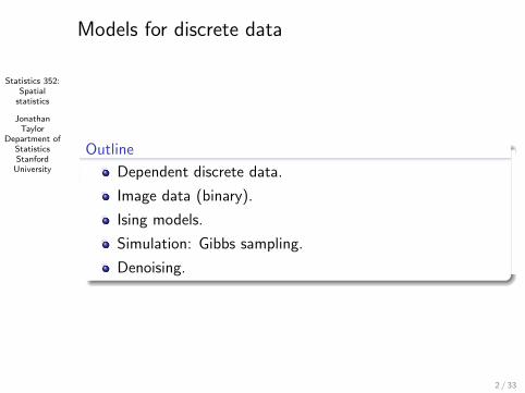
Outline

Dependent discrete data.

Image data (binary).

Ising models.

Simulation: Gibbs sampling.

Denoising.

2 / 33


statistics

JonathanTaylor


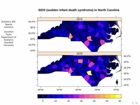
SIDS (sudden infant death syndrome) in North Carolina

34°°N

34.5°°N

35°°N

35.5°°N

36°°N

36.5°°N1974

84°°W 82°°W 80°°W 78°°W 76°°W

34°°N

34.5°°N

35°°N

35.5°°N

36°°N

36.5°°N1979

0 10 20 30 40 50 603 / 33


statistics

JonathanTaylor


Discrete data

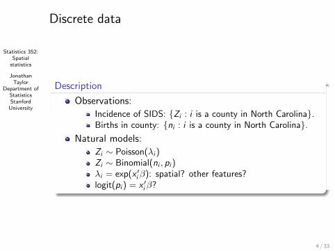
Description

Observations:

Incidence of SIDS: {Zi : i is a county in North Carolina}.Births in county: {ni : i is a county in North Carolina}.

Natural models:

Zi ∼ Poisson(λi )Zi ∼ Binomial(ni , pi )λi = exp(x ′

i β): spatial? other features?logit(pi ) = x ′

i β?

4 / 33


statistics

JonathanTaylor


Discrete data

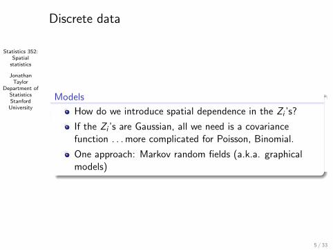
Models

How do we introduce spatial dependence in the Zi ’s?

If the Zi ’s are Gaussian, all we need is a covariancefunction . . . more complicated for Poisson, Binomial.

One approach: Markov random fields (a.k.a. graphicalmodels)

5 / 33


statistics

JonathanTaylor


Discrete data

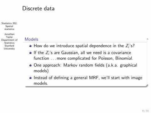
Models

How do we introduce spatial dependence in the Zi ’s?

If the Zi ’s are Gaussian, all we need is a covariancefunction . . . more complicated for Poisson, Binomial.

One approach: Markov random fields (a.k.a. graphicalmodels)

Instead of defining a general MRF, we’ll start with imagemodels.

6 / 33


statistics

JonathanTaylor


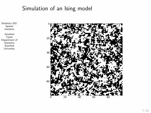
Simulation of an Ising model

7 / 33


statistics

JonathanTaylor


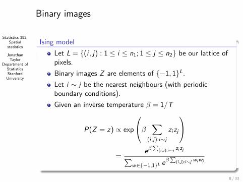
Binary images

Ising model

Let L = {(i , j) : 1 ≤ i ≤ n1; 1 ≤ j ≤ n2} be our lattice ofpixels.

Binary images Z are elements of {−1, 1}L.

Let i ∼ j be the nearest neighbours (with periodicboundary conditions).

Given an inverse temperature β = 1/T

P(Z = z) ∝ exp

β ∑(i ,j):i∼j

zizj

=

eβP

(i,j):i∼j zizj∑w∈{−1,1}L eβ

P(i,j):i∼j wiwj

8 / 33


statistics

JonathanTaylor


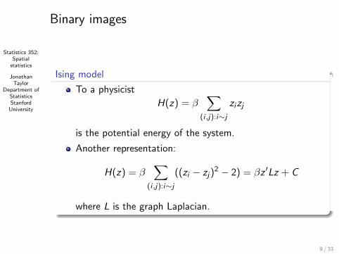
Binary images

Ising model

To a physicist

H(z) = β∑

(i ,j):i∼j

zizj

is the potential energy of the system.

Another representation:

H(z) = β∑

(i ,j):i∼j

((zi − zj)2 − 2) = βz ′Lz + C

where L is the graph Laplacian.

9 / 33


statistics

JonathanTaylor


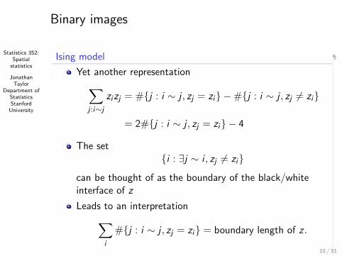
Binary images

Ising model

Yet another representation∑j :i∼j

zizj = #{j : i ∼ j , zj = zi} −#{j : i ∼ j , zj 6= zi}

= 2#{j : i ∼ j , zj = zi} − 4

The set{i : ∃j ∼ i , zj 6= zi}

can be thought of as the boundary of the black/whiteinterface of z

Leads to an interpretation∑i

#{j : i ∼ j , zj = zi} = boundary length of z .

10 / 33


statistics

JonathanTaylor


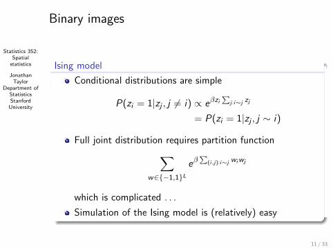
Binary images

Ising model

Conditional distributions are simple

P(zi = 1|zj , j 6= i) ∝ eβziP

j :i∼j zj

= P(zi = 1|zj , j ∼ i)

Full joint distribution requires partition function∑w∈{−1,1}L

eβP

(i,j):i∼j wiwj

which is complicated . . .

Simulation of the Ising model is (relatively) easy

11 / 33


statistics

JonathanTaylor


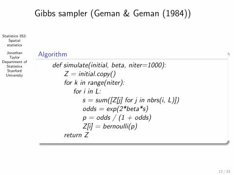
Gibbs sampler (Geman & Geman (1984))

Algorithm

def simulate(initial, beta, niter=1000):Z = initial.copy()for k in range(niter):

for i in L:s = sum([Z[j] for j in nbrs(i, L)])odds = exp(2*beta*s)p = odds / (1 + odds)Z[i] = bernoulli(p)

return Z

12 / 33


statistics

JonathanTaylor


Gibbs sampler

Convergence

For whatever initial configuration initial , as niter →∞

Zniter niter→∞⇒ Zβ

where Zβ is a realization of the Ising model.

In fact, as a process (Z i )1≤i≤niter is a Markov chain thathas stationary distribution Zβ.

This is the basis of most of the MCMC literature . . .

We’ll see the Gibbs sampler again for more general MRFs.

13 / 33


statistics

JonathanTaylor


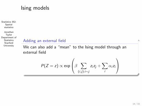
Ising models

Adding an external field

We can also add a “mean” to the Ising model through anexternal field

P(Z = z) ∝ exp

β ∑(i ,j):i∼j

zizj +∑

i

αizi

14 / 33


statistics

JonathanTaylor


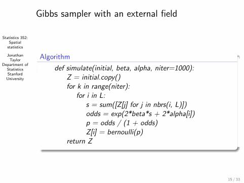
Gibbs sampler with an external field

Algorithm

def simulate(initial, beta, alpha, niter=1000):Z = initial.copy()for k in range(niter):

for i in L:s = sum([Z[j] for j in nbrs(i, L)])odds = exp(2*beta*s + 2*alpha[i])p = odds / (1 + odds)Z[i] = bernoulli(p)

return Z

15 / 33


statistics

JonathanTaylor


Denoising

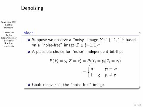
Model

Suppose we observe a “noisy” image Y ∈ {−1, 1}L basedon a “noise-free” image Z ∈ {−1, 1}L

A plausible choice for “noise” independent bit-flips

P(Yi = yi |Z = z) = P(Yi = yi |Zi = zi )

=

{q yi = zi

1− q yi 6= zi

Goal: recover Z , the “noise-free” image.

16 / 33


statistics

JonathanTaylor


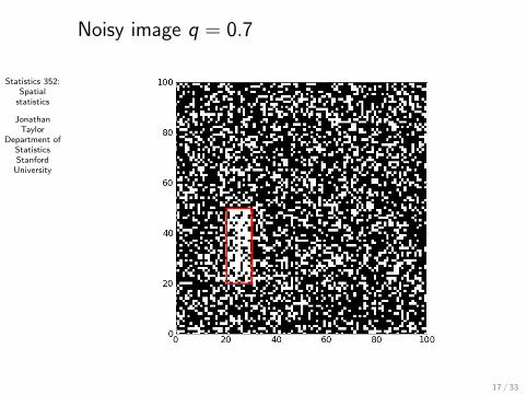
Noisy image q = 0.7

17 / 33


statistics

JonathanTaylor


Denoising

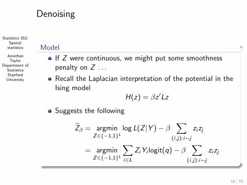
Model

If Z were continuous, we might put some smoothnesspenalty on Z . . .

Recall the Laplacian interpretation of the potential in theIsing model

H(z) = βz ′Lz

Suggests the following

Zβ = argminZ∈{−1,1}L

log L(Z |Y )− β∑

(i ,j):i∼j

zizj

= argminZ∈{−1,1}L

∑i∈L

ZiYi logit(q)− β∑

(i ,j):i∼j

zizj

18 / 33


statistics

JonathanTaylor


Denoising

Model

Our “suggested” estimator is the mode of an Ising modelwith parameter β and field αi = logit(q)Yi . . .

In Bayesian terms, if our prior for Z is Ising withparameter β, the posterior is Ising with a field dependenton the observations Y .

If it’s Bayesian, we can sample from the posterior usingGibbs sampler.

19 / 33


statistics

JonathanTaylor


Denoising

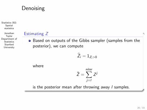
Estimating Z

Based on outputs of the Gibbs sampler (samples from theposterior), we can compute

Zi = 1Zi>0

where

Z =niter∑j=l

Z j

is the posterior mean after throwing away l samples.

20 / 33


statistics

JonathanTaylor


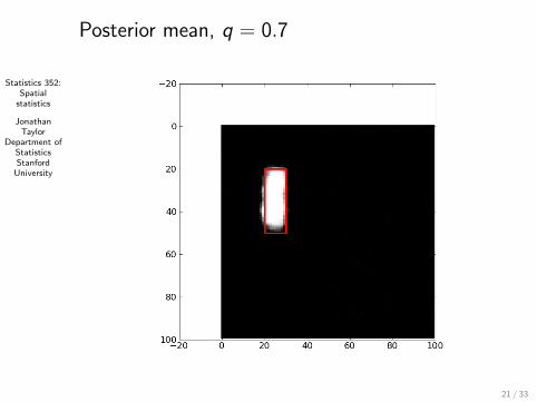
Posterior mean, q = 0.7

21 / 33


statistics

JonathanTaylor


Denoising

Computing the MAP

Our original estimator was the MAP for this prior.

Finding the MAP is a combinatorial optimization problem:{−1, 1}L possible configurations to search through.

A general approach is based on “simulated annealing”.(Geman & Geman, 1984).

22 / 33


statistics

JonathanTaylor


Denoising

Simulated annealing

Basic observation: Zβ(Y ) is also the mode of

PT ,β,Y (z) ∝ exp

− 1

T

β ∑(i ,j):i∼j

zizj − logit(q)∑i∈L

Yizi

BUT, for T > 1, PT ,β,Y is more sharply peaked thanP1,β,Y .

Depends on a choice of temperature schedule . . .

To prove things, one often has to assume Titer = log(iter).

23 / 33


statistics

JonathanTaylor


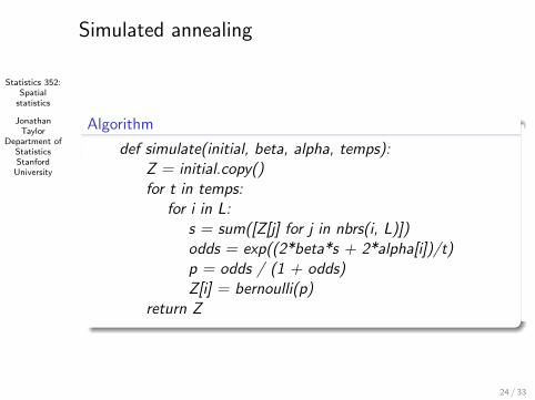
Simulated annealing

Algorithm

def simulate(initial, beta, alpha, temps):Z = initial.copy()for t in temps:

for i in L:s = sum([Z[j] for j in nbrs(i, L)])odds = exp((2*beta*s + 2*alpha[i])/t)p = odds / (1 + odds)Z[i] = bernoulli(p)

return Z

24 / 33


statistics

JonathanTaylor


Denoising

Additive Gaussian noise

Let the new noisy data be

Yi = Zi + εi

with εiIID∼ N(0, σ2)

The field is nowαi = Yizi

and i ∼ i (i.e. a new term in the neighbourhood relation).

25 / 33


statistics

JonathanTaylor


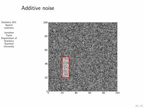
Additive noise

26 / 33


statistics

JonathanTaylor


Additive noise

27 / 33


statistics

JonathanTaylor


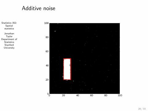
Additive noise

28 / 33


statistics

JonathanTaylor


Denoising

Mixture model

The additive noise example can be thought of as atwo-class mixture model.

Suggests using LDA (or QDA if variances unequal) toclassify.

Problem: the mixing proportion is 0.03...

29 / 33


statistics

JonathanTaylor


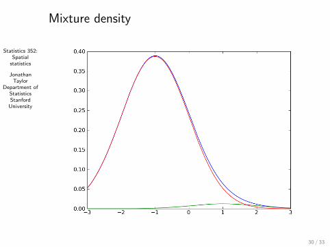
Mixture density

30 / 33


statistics

JonathanTaylor


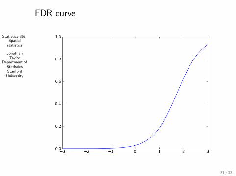
FDR curve

31 / 33


statistics

JonathanTaylor


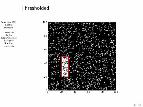
Thresholded

32 / 33


statistics

JonathanTaylor


Where this leaves us

Markov random fields

MRFs generally have distributions “like” an Ising model.

Gibbs sampler can be used to simulate MRFs.

Simulated annealing can also generally be used to findMAP (i.e. modes of an MRF).

Bayesian image analysis is a huge field.

33 / 33

Documents

Statistics 352: Spatial statistics - Models for discrete datastatweb.stanford.edu/~jtaylo/courses/stats352/notes/... · 2009-05-26 · Statistics 352: Spatial statistics Jonathan