Statistical Arbitrage in BalancingMarkets

and the Impact of Time Delay

Stefan Kermer, Derek Bunn

1

Agenda

• Introduction– Austrian Imbalance Settlement Design

– Market Players‘ Perspectives

• Predicting the Conditional Distribution of Imbalance– Quantile Regression Model

– Results with different time delays

• BackTesting Simulations

2

Austrian Imbalance Settlement Design

3

Source: APCS, July 2015

imb

𝑝𝐵𝐴

𝑝 𝐵𝑎𝑠𝑖𝑠

𝑖𝑚𝑏𝑚𝑎𝑥

𝑈𝑚𝑎𝑥

System long System short

Under Production

Short position

Over Production

Long position

𝑝𝐵𝑎𝑠𝑖𝑠

min ptert,pID , pDA for imb<0 and activated tertary

min pID, pDA for imb<0 and no tertiary

max ptert,pID , pDA for imb>0 and activated tertary

max pID, pDA for imb>0 and no tertiary

𝑇 = min(𝑈𝑚𝑖𝑛 +𝑈𝑚𝑎𝑥 − 𝑈𝑚𝑖𝑛

imb𝑚𝑎𝑥2 × 𝑖𝑚𝑏2 ; 𝑈𝑚𝑎𝑥)

𝑝𝐵𝐴 = 𝑝𝐵𝑎𝑠𝑖𝑠 ± 𝑇

Market Player´s Perspectives

4

+

𝑣 = ( 𝑥 𝑖𝑚𝑏 −𝑀𝐶) ∗ 𝑥𝐵𝐴

Pay off function for rational decisions

Needs a rational expectation for 𝑖𝑚𝑏

Information update Imbalance Wind and solar error EPEX spot last price DPI

IL

DI

DI … decision and internal schedule transmission

DPI… delivery period internal schedule changes (15 minutes)

IL… TSO processing information lead time is 10 minutes for imbalance, furthermore we

assume the same lead time for solar-, wind error

IT… Information time delay

IT

Physical Player e.g. gas turbine

IL

DE

DE … decision and internal schedule transmission

DPE… delivery period internal schedule 60 minutes à 15 minutes balancing prices

IL… TSO processing Information lead tim10 minutes for imbalance, furthermore we

assume the same lead time for solar-, wind error

PLE… TSO processing lead time for external schedule nomination (45 minutes)

IT… Information time delay

DPE1 DPE2 DP

E3 DP

E4

PLE

IT

Non-Physical Player (external schedules)

Information perspectiveDecision perspective

Quantile Regression Forecast

5

imbi j = βi1 ∗ imbi j−r + βi2 ∗ EPEXi j−r + βi3 × wind_ei j−r + βi4 ∗ solar_ei j−r + c𝑖

We identified 4 explanatory variables to describe the

response variable 𝑖𝑚𝑏𝑖 𝑗:

𝑖𝑚𝑏𝑖 𝑗−𝑟 Imbalance(j-r) autoregressive parameter with

a time lag of j-r. 𝐸𝑃𝐸𝑋𝑖 𝑗−𝑟Last price EPEX(j-r) EPEX spot intraday

trading closes at j-r. 𝑤𝑖𝑛𝑑_𝑒𝑖 𝑗−𝑟Wind error(j-r) is calculated as the

difference between the day ahead forecast and the actual measured. 𝑠𝑜𝑙𝑎𝑟_𝑒𝑖 𝑗−𝑟Solar error(j-r) is calculated as the

difference between the day ahead forecast and the actual measured value.

𝐼𝑀𝐵 q2.5 q10 q20 q30 q40 q50 q60 q70 q80 iq90 q97.5

Time lags 1 to 8 Parametrizing 2 months (January and July) Outcome: A conditional distribution

Information time delay in [minutes]

Quantile Regression Forecast

6

𝑾𝒉𝒂𝒕 𝒅𝒐 𝒘𝒆 𝒈𝒆𝒕 𝒇𝒓𝒐𝒎 𝒕𝒉𝒂𝒕 𝒂𝒏𝒂𝒍𝒚𝒔𝒊𝒔?

Lag 1 model

Lag 8 model

A more accurate portrayal of the relationship between the response variable and the observed explanatory variables

Expected Value Model

7

𝑚𝑎𝑥𝑘 𝐸𝑉(𝑥𝑘) =

𝑖∈𝐼

𝑣𝑖 𝑘 𝜌(𝑠𝑖)

The expected value for a given course of action is the weighted sum of possible pay offs for each alternative. It is obtained by summing the payoffs for each course of action multiplied by the probabilities 𝜌(𝑠𝑖) associated with each state of nature 𝑠𝑖. The course of action 𝑥𝑘 is chosen which has the highest expected value 𝐸𝑉(𝑥𝑘).

Physical Player

Non-physical player

v𝑙𝑜𝑛𝑔 = ( 𝑖𝑚𝑏 −𝑀𝐶) ∗ 𝑥

v𝑠ℎ𝑜𝑟𝑡 = 𝑀𝐶𝐷𝐴 −𝑝𝑔𝑎𝑠𝑠ℎ𝑜𝑟𝑡 − 𝑝 𝑥 𝑖𝑚𝑏 ) ∗ 𝑥

𝑣 = 𝑝 𝑥. 𝑖𝑚𝑏 − 𝑀𝐶𝐸𝑃𝐸𝑋 ∗ 𝑥

ma k(𝑗

𝑖∈𝐼

𝑣𝑖 𝑗 𝑘 ∗ 𝜌( 𝑖𝑚𝑏𝑖) )

Pay offs:

OUR OBJECTIVE:

Index for time 𝑗 ∈ {T}

Index for state of nature 𝑖 ∈𝐼𝑀𝐵

Index for position 𝑘 ∈ {−100…0. . +100} in MWh

Assumption:Physical player is in part-load

Assumption:Non-Physical player trades last price at EPEX Spot

Back Testing with observed datawinter and summer month 2015Benchmark and key performanceindicators

Results Physical/Non-Physical Player

8

-

500.000

1.000.000

1.500.000

2.000.000

2.500.000

realizedprofit

expectedprofit

realizedprofit

expectedprofit

summer summer winter winter

pro

fit

[EU

R/m

on

th]

physical player non-physical player

-

500.000

1.000.000

1.500.000

2.000.000

2.500.000

3.000.000

summer wintersyst

em

co

sts

in [

EUR

/mo

nt]

observation physical player non-physical player

20,00

22,00

24,00

26,00

28,00

30,00

32,00

summer winterstan

dar

d d

evi

atio

n in

[M

Wh

]

observation physical player non-physical player

48.000 50.000 52.000 54.000 56.000 58.000 60.000 62.000 64.000 66.000

winter summer

abso

lute

imb

alan

ce in

[M

Wh

]

observation physical player non-physical player

Results Physical/Non-Physical Player

9

physical player non-physical player

short positions winter 380 1641

short positions summer 271 1466

long positions winter 63 867

long positions summer 53 1050

Dynamic Analysis

10

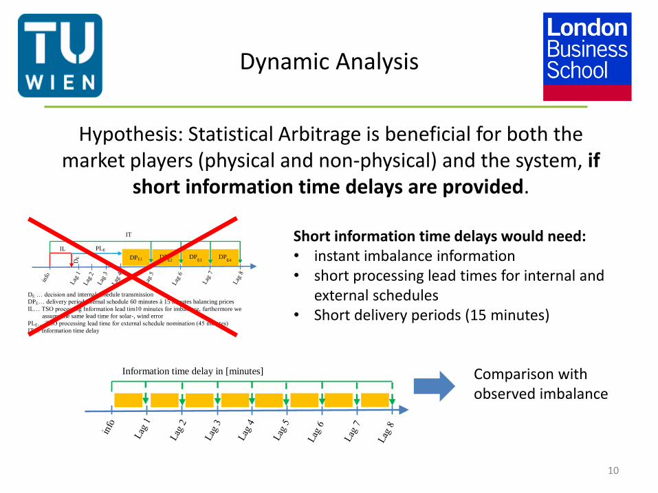
Hypothesis: Statistical Arbitrage is beneficial for both the market players (physical and non-physical) and the system, if

short information time delays are provided.

Short information time delays would need:• instant imbalance information• short processing lead times for internal and

external schedules• Short delivery periods (15 minutes)

IL

DE

DE … decision and internal schedule transmission

DPE… delivery period internal schedule 60 minutes à 15 minutes balancing prices

IL… TSO processing Information lead tim10 minutes for imbalance, furthermore we

assume the same lead time for solar-, wind error

PLE… TSO processing lead time for external schedule nomination (45 minutes)

IT… Information time delay

DPE1 DPE2 DP

E3 DP

E4

PLE

IT

Information time delay in [minutes] Comparison withobserved imbalance

Dynamic Analysis Non-Physical PlayerSystem Costs and Parameters

11

Financial and system behavioural metrics show a win-win situation

WINTER SUMMERSystem costs System costs

Absolute imbalance Standard deviation

System costs System costs

Absolute imbalance Standard deviation

Dynamic Analysis Non-Physical PlayerSystem Costs and Parameters

12

With long information time delays the actions are inefficient.

WINTER SUMMERSystem costs System costs

Absolute imbalance Standard deviation

System costs System costs

Absolute imbalance Standard deviation

Dynamic Analysis Non-Physical PlayerHow often did they take positions?

13

0%10%20%30%40%50%60%70%

qu

anti

ty s

um

me

r

short positions non-physical player wintershort positions physical player winterlong positions non-physical player winterlong positions physical player winter

0%10%20%30%40%50%60%70%

qu

anti

ty s

um

me

r

short positions non-physical player wintershort positions physical player winterlong positions non-physical player winterlong positions physical player winter

0%

10%

20%

30%

40%

50%

60%

70%

80%

90%

100%

pe

rce

nta

ge o

f p

osi

tio

ns

quantity of positions non-physical player summer

quantity of positions non-physical player winter

quantity of positions physical player summer

quantity of positions physical player winter

How often do theyspill/short themarket?

From 2683 15 minute intervals in winter/summer thephysical player traded less than 20 percent of time intervals whereas the non-physical EPEX Spot trading model suggested over 90% of the time to take a imbalance position.

Dynamic Analysis Non-Physical PlayerImbalance Extremes

14

WINTER SUMMER

imb

𝑝𝐵𝐴

𝑝 𝐵𝑎𝑠𝑖𝑠

𝑖𝑚𝑏𝑚𝑎𝑥

𝑈𝑚𝑎𝑥

System long System short

Under Production

Short position

Over Production

Long position

System long >70 MWh decreased significantlySystem Short >70 MWh remained constant for physicalplayer and increased slightly for non-physical player

Dynamic Analysis Non-Physical PlayerImbalance Half-cycles

15

- 100 200 300 400 500 600 700 800 900

1.000

imb

alan

ce h

alf

cycl

es

[-]

half cycles winter half cycles summer

Half cycles in case of participation of the physical player increased by 80% for the lag 1 modelFor the physical player only a slight increase is observed.

Conclusion

16

Research Questions:Does statistical arbitrage help the system to decrease system imbalance and system costs? What is the impact of information time delay?

For the physical player YES! Short time delays decrease system costs and stabilize the

system significantly.

For the non-physical player a more differentiated point of view is necessary:

• The current nomination regulation offers arbitrage potential for the non-physical player(profitpotential), but it is not as beneficial from system perspective

• In the dynamic analysis we observed a significant reduction of imbalance extremes if the system imbalance was long, but a slight increase for short imbalance extremes

• Furthermore we saw that up to a time lag of 30 minutes the non-physical player wouldbe able to help the system, but the frequency of trades in this single player simulationwas very high, which potentially would lead to overreactions in the market in a multiplayer setting.

BACK UP

• In August, 2 short extremes can be described by LAST Epex spot price extremes

17

REF Time

OLS IMB

EST

OLS_pBA_i

mb_est_N

O_x

OLS_pBA_d

ec x-decision imbalance_obs imb_obs+x obs_pBA_BASE

obs_pBA_Op

timized_no_t

ert

expected

spread spread p_ID

20908 557 8,63 60,03 -00 100,00 0,71 100,71 59,54 96,54 -180,00 83,46 180,00

22851 2500 -15,83 13,35 -00 100,00 -37,08 62,92 5,95 66,42 -198,00 131,58 198,00