Embed Size (px)
Citation preview
Realized GARCH: A Joint Model for Returns and Realized
Measures of Volatility∗
Peter Reinhard Hansen† Zhuo Huang‡ Howard Howan Shek§
November 2, 2010
Abstract
We introduce a new framework, Realized GARCH, for the joint modeling of returns and realized
measures of volatility. A key feature is a measurement equation that relates the realized measure to
the conditional variance of returns. The measurement equation facilitates a simple modeling of the
dependence between returns and future volatility. Realized GARCH models with a linear or log-linear
speci�cation have many attractive features. They are parsimonious, simple to estimate, and imply an
ARMA structure for the conditional variance and the realized measure. An empirical application with
DJIA stocks and an exchange traded index fund shows that a simple Realized GARCH structure leads to
substantial improvements in the empirical �t over standard GARCH models that only use daily returns.
Keywords: GARCH; High Frequency Data; Realized Variance; Leverage E�ect.
JEL Classi�cation: C10; C22; C80
∗We thank Tim Bollerslev, Giampiero Gallo, Asger Lunde, and seminar participants at Humboldt University, the EinaudiInstitute, the 2009 Stanford Institute for Theoretical Economics, and the Volatility Institute at New York University SternSchool of Business for valuable comments.†Stanford University, Department of Economics & CREATES.‡Peking University, China Center for Economic Research, National School of Development & Stanford University§Stanford University, iCME.
1
1 Introduction
The latent volatility process of asset returns is relevant for a wide variety of applications, such as option pricing
and risk management, and GARCH models are widely used to model the dynamic features of volatility. This
has sparked the development of a large number of ARCH and GARCH models since the seminal paper
by Engle (1982). Within the GARCH framework, the key element is the speci�cation for the conditional
variance. Standard GARCH models utilize daily returns (typically squared returns) to extract information
about the current level of volatility, and this information is used to form expectations about the next period's
volatility. A single return only o�ers a weak signal about the current level of volatility. The implication is
that GARCH models are poorly suited for situations where volatility changes rapidly to a new level. The
reason is that a GARCH model is slow at �catching up� and it will take many periods for the conditional
variance (implied by the GARCH model) to reach its new level, as discussed in Andersen et al. (2003).
High-frequency �nancial data are now widely available and the literature has recently introduced a number
of realized measures of volatility, including the realized variance, the bipower variation, the realized kernel,
and many related quantities, see Andersen and Bollerslev (1998), Andersen, Bollerslev, Diebold, and Labys
(2001), Barndor�-Nielsen and Shephard (2002, 2004), , Barndor�-Nielsen, Hansen, Lunde, and Shephard
(2008), Andersen et al. (2008), Hansen and Horel (2009) and references therein. Any of these measures is
far more informative about the current level of volatility than is the squared return. This makes realized
measures very useful for modeling and forecasting future volatility. Estimating a GARCH model that includes
a realized measure in the GARCH equation (known as a GARCH-X model) provides a good illustration of
this point. Such models were estimated by Engle (2002) who used the realized variance, see also Forsberg and
Bollerslev (2002). Within the GARCH-X framework no e�ort is paid to explain the variation in the realized
measures, so these GARCH-X models are partial (incomplete) models that have nothing to say about returns
and volatility beyond a single period into the future.
Engle and Gallo (2006) introduced the �rst �complete� model in this context. Their model speci�es
a GARCH structure for each of the realized measures, so that an additional latent volatility process is
introduced for each realized measure in the model. The model by Engle and Gallo (2006) is known as the
Multiplicative Error Model (MEM), because it builds on the MEM structure proposed by Engle (2002).
Another complete model is the HEAVY model by Shephard and Sheppard (2010) that, in terms of its
mathematical structure, is nested in the MEM framework. Unlike the traditional GARCH models, these
models operate with multiple latent volatility processes. For instance, the MEM by Engle and Gallo (2006)
has a total of three latent volatility processes and the HEAVY model by Shephard and Sheppard (2010) has
two (or more) latent volatility processes. Within the context of stochastic volatility models, Takahashi et al.
(2009) proposed a joint model for returns and a realized measure of volatility. Importantly, the economic and
statistical gains from incorporating realized measures in volatility models are typically found to be large, see
e.g. Christo�ersen et al. (2010) and Dobrev and Szerszen (2010).
In this paper we introduce a new framework that combines a GARCH structure for returns with an
2
integrated model for realized measures of volatility. Models within our framework are called Realized GARCH
models, a name that transpires both the objective of these models (similar to GARCH) and the means by
which these models operate (using realized measures).
To illustrate our framework and �x ideas, consider a canonical version of the Realized GARCH model
that will be referred to as the RealGARCH(1,1) model with a linear speci�cation. This model is given by
the following three equations
rt =√htzt,
ht = ω + βht−1 + γxt−1,
xt = ξ + ϕht + τ(zt) + ut,
where rt is the return, xt a realized measure of volatility, zt ∼ iid(0, 1), ut ∼ iid(0, σ2u), and ht = var(rt|Ft−1)
with Ft = σ(rt, xt, rt−1, xt−1, . . .). The last equation relates the observed realized measure to the latent
volatility, and is therefore called the measurement equation. This equation is natural when xt is a consistent
estimator of the integrated variance, because the integrated variance may be viewed as the conditional
variance plus a random innovation. The latter is, in our model, absorbed by τ(zt) + ut. It is easy to verify
that ht is an autoregressive process of order one, ht = µ + πht−1 + wt−1, where µ = ω + γξ, π = β + ϕγ,
and wt = γτ(zt) + γut. So it is natural to adopt the nomenclature of GARCH (generalized autoregressive
conditional heteroskedasticity) models. The inclusion of the realized measure in the model and the fact that
xt has an autoregressive moving average (ARMA) representation motivate the name Realized GARCH. A
simple, yet potent speci�cation of the leverage function is τ(z) = τ1z + τ2(z2 − 1), which can generate an
asymmetric response in volatility to return shocks. The simple structure of the model makes the model easy
to estimate and interpret, and leads to a tractable analysis of the quasi maximum likelihood estimator. The
framework allows us to use a realized measure that is computed from a shorter period (e.g. 6.5 hours) than
the interval that the conditional variance refers to (e.g. 24 hours). In such instances we should expect ϕ < 1.
We apply the Realized GARCH framework to the DJIA stocks and an exchange traded index fund, SPY.
We �nd, in all cases, substantial improvements in the log-likelihood function (both in-sample and out-of-
sample) when benchmarked to a standard GARCH model. This is not too surprising, because the standard
GARCH model is based on a more limited information set that only includes daily returns. The empirical
evidence strongly favors inclusion of the leverage function, and the parameter estimates are remarkably similar
across stocks.
The paper is organized as follows. Section 2 introduces the Realized GARCH framework as a natural
extension to GARCH. We focus on linear and log-linear speci�cation and show that squared returns, the
conditional variance, and realized measures have ARMA representations in this class of Realized GARCH
models. Our Realized GARCH framework is compared to MEM and related models in Section 3. Likelihood-
based inference is analyzed in Section 4, where we derive the asymptotic properties of the QMLE estimator.
Our empirical analysis is given in Section 5. We estimate a range of Realized GARCH models using time
3
series for 28 stocks and an exchange traded index fund. In Section 6 we derive results related to forecasting
and the skewness and kurtosis of returns over one or more periods. The latter shows that the Realized
GARCH is capable of generating substantial skewness and kurtosis. Concluding remarks are given in Section
7, and Appendix A presents all proofs.
2 Realized GARCH
In this section we introduce the Realized GARCH model. The key variable of interest is the conditional
variance, ht = var(rt|Ft−1), where {rt} is a time series of returns. In the GARCH(1,1) model the conditional
variance, ht, is a function of ht−1 and r2t−1. In the present framework, ht will also depend on xt−1, that
represents a realized measure of volatility, such as the realized variance. More generally, xt will denote a
vector of realized measures, such as the realized variance, the bipower variation, the intraday range, and the
squared return. A measurement equation, which ties the realized measure to the latent volatility, �completes�
the model. So the Realized GARCH model fully speci�es the dynamic properties of both returns and the
realized measure.
To simplify the exposition we will assume E(rt|Ft−1) = 0. A more general speci�cations for the conditional
mean, such as a constant or the GARCH-in-mean by Engle et al. (1987), is accommodated by reinterpreting
rt as the return less its conditional mean. The general framework for the Realized GARCH model is presented
next.
2.1 The General Formulation
The general structure of the RealGARCH(p,q) model is given by
rt =√htzt, (1)
ht = v(ht−1, . . . , ht−p, xt−1, . . . , xt−q), (2)
xt = m(ht, zt, ut), (3)
where zt ∼ iid (0, 1) and ut ∼ iid (0, σ2u), with zt and ut being mutually independent.
We refer to the �rst two equations as the return equation and the GARCH equation, and these de�ne
a class of GARCH-X models, including those that were estimated by Engle (2002), Barndor�-Nielsen and
Shephard (2007), and Visser (2010). The GARCH-X acronym refers to the the fact that xt is treated as
an exogenous variable. The HYBRID GARCH framework by Chen et al. (2009) includes variants of the
GARCH-X models and some related models.
We shall refer to (3) as the measurement equation, because the realized measure, xt, can often be in-
terpreted as a measurement of ht. The simplest example of a measurement equation is: xt = ht + ut. The
measurement equation is an important component because it �completes� the model. Moreover, the measure-
ment equation provides a simple way to model the joint dependence between rt and xt, which is known to be
4
empirically important. This dependence is modeled though the presence of zt in the measurement equation,
which we �nd to be highly signi�cant in our empirical analysis.
It is worth noting that most (if not all) variants of ARCH and GARCH models are nested in the Realized
GARCH framework. See Bollerslev (2009) for a comprehensive list of such models. The nesting can be
achieved by setting xt = rt or xt = r2t , and the measurement equation is redundant for such models, because
it is reduced to a simple identity. Naturally, the interesting case is when xt is a high-frequency based realized
measure, or a vector containing several realized measures. Next we consider some particular variants of the
Realized GARCH model.
2.2 Realized GARCH with a Log-Linear Speci�cation
The Realized GARCH model with a simple log-linear speci�cation is characterized by the following GARCH
and measurement equations.
log ht = ω +∑p
i=1βi log ht−i +
∑q
j=1γj log xt−j , (4)
log xt = ξ + ϕ log ht + τ(zt) + ut, (5)
where zt = rt/√ht ∼ iid (0, 1), ut ∼ iid (0, σ2
u), and τ(z) is called the leverage function. Without loss of
generality we assume Eτ(zt) = 0.
A logarithmic speci�cation for the measurement equation seems natural in this context. The reason is
that (1) implies that
log r2t = log ht + log z2t , (6)
and a realized measure is in many ways similar to the squared return, r2t , albeit a more accurate measure
of ht. It is therefore natural to explore speci�cations where log xt is expressed as a function of log ht and zt,
such as (5). A logarithmic form for the measurement equation makes it convenient to specify the GARCH
equation with a logarithmic form, because this induces a convenient ARMA structure.
In our empirical application we adopt a quadratic speci�cation for the leverage function, τ(zt). The
conditional variance, ht is adapted to Ft−1. So Ft must be such that xt ∈ Ft (unless γ = 0). This requirement
is satis�ed with, Ft = σ(rt, xt, rt−1, xt−1, . . .), but Ft could in principle be an even richer σ-�eld. Also, note
that the measurement equation does not require xt to be an unbiased measure of ht. For instance, xt could be
a realized measure that is computed with 6.5 hours of high-frequency data while the return is a close-to-close
return that spans 24 hours.
An attractive feature of the log-linear Realized GARCH model is that it preserves the ARMA structure
that characterizes some of the standard GARCH models. This shows that the �ARCH� nomenclature is
appropriate for the Realized GARCH model. For the sake of generality we derive the result for the case
where the GARCH equation includes lagged squared returns. Thus consider the following GARCH equation,
5
log ht = ω +∑p
i=1βi log ht−i +
∑q
j=1γj log xt−j +
∑q
j=1αj log r2t−j , (7)
where q = maxi{(αi, γi) 6= (0, 0)}.
Proposition 1. De�ne wt = τ(zt) +ut and vt = log z2t −κ, where κ = E log z2t . The Realized GARCH model
de�ned by (5) and (7) implies
log ht = µh +
p∨q∑i=1
(αi + βi + ϕγi) log ht−i +
q∑j=1
(γjwt−j + αjvt−j),
log xt = µx +
p∨q∑i=1
(αi + βi + ϕγi) log xt−i + wt +
p∨q∑j=1
{−(αj + βj)wt−j + ϕαjvt−j} ,
log r2t = µr +
p∨q∑i=1
(αi + βi + ϕγi) log r2t−i + vt +
p∨q∑j=1
{γi(wt−j − ϕvt−j)− βjvt−j} ,
where µh = ω + γ•ξ + α•κ, µx = ϕ(ω + α•κ) + (1 − α• − β•)ξ, and µr = ω + γ•ξ + (1 − β• − ϕγ•)κ, with
α• =∑qj=1 αj, β• =
∑pi=1 βi, and γ• =
∑qj=1 γj, and the conventions βi = γj = αj = 0 for i > p and j > q.
So the log-linear Realized GARCH model implies that log ht is ARMA(p ∨ q, q − 1), whereas log r2t and
log xt are ARMA(p ∨ q, p ∨ q). If α1 = · · · = αq = 0, then log xt is ARMA(p ∨ q, p).
From Proposition 1 we see that the persistence of volatility is summarized by a persistence parameter
π =
p∨q∑i=1
(αi + βi + ϕγi) = α• + β• + ϕγ•.
Example 1. For the case p = q = 1 we have log ht = ω + β log ht−1 + γ log xt−1 and log xt = ξ + ϕ log ht +
τ(zt) + ut, so that log ht ∼AR(1) and log xt ∼ARMA(1,1). Speci�cally log ht = µh + π log ht−1 + γwt−1 and
log xt = µx + π log xt−1 + wt − βwt−1, where π = β + ϕγ.
The measurement equation induces a GARCH structure that is similar to an EGARCH with a stochastic
volatility component. Take the case in Example 1 where log ht = µh+π log ht−1+γτ(zt−1)+γut−1. Note that
γτ(zt−1) captures the leverage e�ects whereas γut−1 adds an additional stochastic component that resembles
that of stochastic volatility models. So the Realized GARCH model can induce a �exible stochastic volatility
structure, similar to that in Yu (2008), but does in fact have a GARCH structure because ut−1 is Ft−1-
measurable. Interestingly, for the purpose of forecasting (beyond one-step ahead predictions), the Realized
GARCH is much like a stochastic volatility model since future values of ut are unknown. This analogy does
not apply to one-step ahead predictions because the lagged values, τ(zt−1) and ut−1, are known at time t−1.
An obvious advantage of using a logarithmic speci�cation is that it automatically ensures a positive vari-
ance. Here it should be noted that the GARCH model with a logarithmic speci�cation, known as LGARCH,
see Geweke (1986), Pantula (1986), and Milhøj (1987), has some practical drawbacks. These drawbacks may
6
explain that the LGARCH is less popular in applied work than the conventional GARCH model that uses a
speci�cation for the level of volatility, see Teräsvirta (2009). One drawback is that zero returns occasionally
are observed, and such will cause havoc for the log-speci�cation unless we impose some ad-hoc censoring.
Within the Realized GARCH framework, zero returns are not problematic, because log r2t−1 does not appear
in its GARCH equation.
2.2.1 The Leverage Function
The function τ(z) is called the leverage function because it captures the dependence between returns and
future volatility, a phenomenon that is referred to as the leverage e�ect. We normalize such functions by
Eτ(zt) = 0, and we focus on those that have the form
τ(zt) = τ1a1(zt) + · · ·+ τkak(zt), where Eak(zt) = 0, for all k,
so that the function is linear in the unknown parameters. We shall see that the leverage function induces
an EGARCH type structure in the GARCH equation, and we note that the functional form used in Nelson
(1991), τ(zt) = τ1z + τ+(|zt| − E|zt|) is within this class of leverage functions. In this paper we focus on
leverage functions that are constructed from Hermite polynomials, i.e.
τ(z) = τ1z + τ2(z2 − 1) + τ3(z3 − 3z) + τ4(z4 − 6z2 + 3) + · · · ,
and our baseline choice for the leverage function is a simple quadratic form τ(zt) = τ1zt + τ2(z2t − 1). This
choice is convenient because it ensures that Eτ(zt) = 0, for any distribution with Ezt = 0 and var(zt) = 1.
The polynomial form is also convenient in our quasi-likelihood analysis, and in our derivations of the kurtosis
of returns generated by this model.
The leverage function τ(z) is closely related to the news impact curve, see Engle and Ng (1993), that
maps out how positive and negative shocks to the price a�ect future volatility. We can de�ne the news
impact curve by ν(z) = E(log ht+1|zt = z)−E(log ht+1), so that 100ν(z) measures the percentage impact on
volatility as a function of the studentized return. From the ARMA representation in Proposition 1 it follows
that ν(z) = γ1τ(z).
2.3 Realized GARCH with a Linear Speci�cation
In this section we adopt a linear structure that is more similar to the original GARCH model, by Bollerslev
(1986). One advantage of this formulation is that the measurement equation is simple to interpret in this
model. For instance if xt is computed from intermittent high-frequency data (i.e. over 6.5 hours) whereas rt
is a close-to-close return that spans 24 hours. Then we would expect ϕ to re�ect how much of daily volatility
7
that occurs during the trading hours. The linear Realized GARCH model is de�ned by,
xtht = ω +∑p
i=1βiht−i +
∑q
j=1γjxt−j , and = ξ + ϕht + τ(zt) + ut,
As is the case for the GARCH(1,1) model the RealGARCH(1,1) model with the linear speci�cation implies
that ht has an AR(1) representation ht = (ω + γξ) + (β + γϕ)ht−1 + γwt−1, where wt = ut + τ(zt) is an iid
process, and that the realized measure, xt, is ARMA(1,1), which is consistent with the time-series properties
of realized measures in this context, see Meddahi (2003).
3 Comparison to Related Models
In this section we relate the Realized GARCH model to the Multiplicative Error Model (MEM) by Engle
and Gallo (2006) and the HEAVY model by Shephard and Sheppard (2010),1 and some related approaches.
The MEM by Engle and Gallo (2006) utilizes two realized measures in addition to the squared returns.
These are the intraday range (high minus low) and the realized variance, whereas the HEAVY model by
Shephard and Sheppard (2010) uses the realized kernel (RK) by Barndor�-Nielsen et al. (2008). These
models introduce an additional latent volatility process for each of the realized measures. So the MEM and
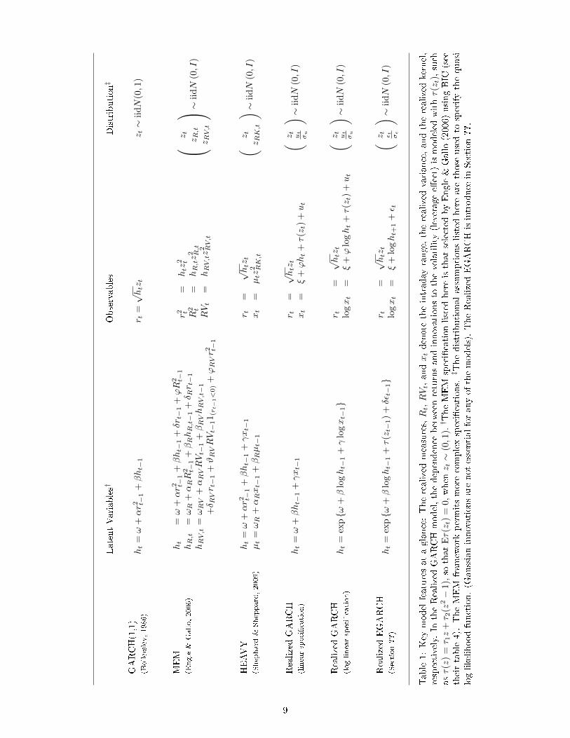
the HEAVY digress from the traditional GARCH models that only have a single latent volatility factor. Key
model features are given in Table 1. We have included the level speci�cation of the Realized GARCH model
because it is most similar to the GARCH, MEM, and HEAVY models. Based on our empirical analysis in
Section 5 we recommend the log-linear speci�cation in practice.
Brownless and Gallo (2010) estimates a restricted MEM model that is closely related to the Realized
GARCH with the linear speci�cation. They utilize a single realized measure, which leads to two latent
volatility processes in their model, ht = E(r2t |Ft−1) and µt = E(xt|Ft−1). However, their model is e�ectively
reduced to a single factor model as they introduce the constraint, ht = c+ dµt.
The usual MEM formulation is based on a vector of non-negative random innovations, ηt, that are required
to have mean E(ηt) = (1, . . . , 1)′. The literature has explored distributions with this property such as certain
multivariate Gamma distributions, and Cipollini, Engle, and Gallo (2009) use copula methods that entail
a very �exible class of distributions with the required structure. (A perhaps simpler way to achieve this
structure is by setting ηt = Zt � Zt, and work with the vector of mean-zero unit-variance random variables,
Zt, instead.) The estimates in Engle and Gallo (2006) and Shephard and Sheppard (2010) are based on
a likelihood where the elements of ηt are independent χ2-distributed random variables with one degree of
freedom, which maps into Zt ∼ N(0, I). We have used the alternative formulation in Table 1 so that
(z2t , z2R,t, z
2RV,t)
′ corresponds to ηt in the MEM by Engle and Gallo (2006).
1The Realized GARCH model was conceptualized and developed concurrently and independently of Shephard and Sheppard(2010). However, in our current presentation of the model we have adopted some terminology from Shephard and Sheppard(2010).
8
LatentVariables†
Observables
Distribution‡
GARCH(1,1)
(Bollerslev,1986)
ht
=ω
+αr2 t−1
+βht−
1r t
=√htz t
z t∼
iidN
(0,1
)
MEM
(Engle&Gallo,2006)
ht
=ω
+αr2 t−1
+βht−
1+δrt−
1+ϕR
2 t−1
hR,t
=ωR
+αRR
2 t−1
+βRhR,t−1
+δ Rr t−1
hRV,t
=ωRV
+αRVRVt−
1+βRVhRV,t−1
+δ RVr t−1
+ϑRVRVt−
11 (rt−
1<0)
+ϕRVr2 t−1
r2 t=
htz2 t
R2 t
=hR,tz2 R,t
RVt
=hRV,tz2 RV,t
z t z R,t
z RV,t
∼ii
dN
(0,I
)
HEAVY
(Shephard
&Sheppard,2009)
ht
=ω
+αr2 t−1
+βht−
1+γxt−
1
µt
=ωR
+αRxt−
1+βRµt−
1
r t=
√htz t
xt
=µtz2 RK,t
(z t
z RK,t
) ∼ii
dN
(0,I
)
RealizedGARCH
(linearspeci�cation)
ht
=ω
+βht−
1+γxt−
1r t
=√htz t
xt
=ξ
+ϕht
+τ(zt)
+ut
( ztut
σu
) ∼ii
dN
(0,I
)
RealizedGARCH
(log-linearspeci�cation)
ht
=ex
p{ω
+β
loght−
1+γ
logxt−
1}
r t=√htz t
logxt
=ξ
+ϕ
loght
+τ(zt)
+ut
( ztut
σu
) ∼ii
dN
(0,I
)
RealizedEGARCH
(Section??)
ht
=ex
p{ω
+β
loght−
1+τ(zt−
1)
+δεt−
1}
r t=√htz t
logxt
=ξ
+lo
ght+
1+ε t
( z t ε t σ ε) ∼
iidN
(0,I
)
Table1:Key
modelfeaturesataglance:Therealizedmeasures,Rt,RVt,andxtdenote
theintraday
range,therealizedvariance,andtherealizedkernel,
respectively.In
theRealizedGARCHmodel,thedependence
betweenreturnsandinnovationsto
thevolatility
(leveragee�ect)
ismodeled
withτ(zt),such
asτ(z
)=τ 1z
+τ 2
(z2−
1),so
that
Eτ(zt)
=0,when
z t∼
(0,1
).† T
heMEM
speci�cationlisted
hereisthatselected
byEngle&Gallo(2006)usingBIC
(see
theirtable4).
TheMEM
framew
ork
permitsmore
complexspeci�cations.‡ T
hedistributionalassumptionslisted
hereare
those
usedto
specifythequasi
log-likelihoodfunction.(G
aussianinnovationsare
notessentialforanyofthemodels).TheRealizedEGARCHisintroduce
inSection??.
9
3.1 Multi-Factor Realized GARCH Models
The Realized GARCH framework can be extended to a multi-factor structure. For instance with m realized
measures (including the squared return) we could specify a model with k ≤ m latent volatility factors.
The Realized GARCH model introduced in this paper has k = 1 whereas the MEM has m = k. This hybrid
framework with 1 ≤ k ≤ m, provides a way to bridge the Realized GARCH models with the MEM framework.
All these models can be viewed as extensions of standard GARCH models, where the extensions are achieved
by incorporating realized measures into the model in various ways.2
4 Quasi-Maximum Likelihood Analysis
In this section we discuss the asymptotic properties of the quasi-maximum likelihood estimator within the
Realized GARCH(p, q) model. The structure of the QMLE analysis is very similar to that of the standard
GARCH model, see Bollerslev and Wooldridge (1992), Lee and Hansen (1994), Lumsdaine (1996), Jensen
and Rahbek (2004a,b), and Straumann and Mikosch (2006). Both Engle and Gallo (2006) and Shephard and
Sheppard (2010) justify the standard errors they report, by referencing existing QMLE results for GARCH
models. This argument hinges on the fact that the joint log-likelihood in the MEM is decomposed into a
sum of univariate GARCH-X models, whose likelihood can be maximized separately. The factorization of
the likelihood is achieved by two facets of these models: One is that all observables (i.e. squared return and
each of the realized measures) are being tied to their individual latent volatility process. The other is that
the primitive innovations in these models are taken to be independent in the formulation of the likelihood
function. The latter inhibits a direct modeling of leverage e�ect with a function such as τ(zt), which is one
of the traits of the Realized GARCH model. However, in the MEM framework one can generate a leverage
type dependence by including suitable realized measures in various GARCH equations, such as the realized
semivariance, see Barndor�-Nielsen et al. (2009b), or by introducing suitable indicator functions as in Engle
and Gallo (2006).
In this section we will derive the underlying QMLE structure for the log-linear Realized GARCH model.
The structure of the linear Realized GARCH model is similar. We provide closed-form expressions for the
�rst and second derivatives of the log-likelihood function. These expressions facilitate direct computation of
robust standard errors, and provide insight about regularity conditions that would justify QMLE inference.
For instance, the �rst derivative will unearth regularity conditions that enable a central limit theorem be
applied to the score function.
For the purpose of estimation, we adopt a Gaussian speci�cation, so that the log likelihood function is
given by
`(r, x; θ) = −1
2
n∑t=1
[log(ht) + r2t /ht + log(σ2u) + u2t/σ
2u].
2A realized measure simply refers to a statistic that is constructed from high-frequency data. Well known examples include:the realized variance, the realized kernel, intraday range, the number of transactions, and trading volume.
10
We write the leverage function as τ ′at = τ1a1(zt) + · · · + τkak(zt), and denote the parameters in the model
by
θ = (λ′, ψ′, σ2u)′, where λ = (ω, β1, . . . , βp, γ1, . . . , γq)
′, ψ = (ξ, ϕ, τ ′)′.
To simplify the notation we write ht = log ht and xt = log xt, and de�ne gt = (1, ht−1, . . . , ht−p, xt−1, . . . , xt−q)′
and mt = (1, ht, a′t)′. So the GARCH and measurement equations can be expresses as ht = λ′gt and
xt = ψ′mt + ut, respectively. The dynamics that underlies the score and Hessian are driven by ht and its
derivatives with respect to λ. The properties of these derivatives are stated next.
Lemma 1. De�ne ht = ∂ht∂λ and ht = ∂2ht
∂λ∂λ′ . Then hs = 0 and hs = 0 for s ≤ 0, and
ht =
p∑i=1
βiht−i + gt and ht =
p∑i=1
βiht−i + (Ht−1 + H ′t−1),
where Ht−1 =(
01+p+q×1, ht−1, . . . , ht−p, 01+p+q×q
)is a p+ q + 1× p+ q + 1 matrix.
Proposition 2. (i) The score, ∂`∂θ =
n∑t=1
∂`t∂θ , is given by
∂`t∂θ
= −1
2
{(1− z2t +
2utσ2u
ut)ht,−2utσ2u
mt,σ2u − u2tσ4u
}′,
where ut = ∂ut/∂ log ht = −ϕ+ 12ztτ
′at with at = ∂a(zt)/∂zt.
(ii) The second derivative, ∂2`∂θ∂θ′ =
n∑t=1
∂2`t∂θ∂θ′ , is given by
∂2`t∂θ∂θ′
=
− 1
2
{z2t +
2(u2t+utut)σ2u
}hth′t − 1
2
{1− z2t + 2utut
σ2u
}ht • •
utσ2umth
′t + ut
σ2ubth′t − 1
σ2umtm
′t •
ututσ4uh′t
utσ4um′t
12σ2u−2u
2t
σ6u
,
where bt = (0, 1,− 12zta
′t)′ and ut = − 1
4τ′ {ztat + z2t at
}with at = ∂2a(zt)/∂z
2t .
An advantage of our framework is that we can draw upon results for generalized hidden Markov models.
Consider the case p = q = 1. From Carrasco and Chen (2002, proposition 2) it follows that ht has a
stationary representation provided that π = β+ϕγ ∈ (−1, 1). If we assign h0 its invariant distribution, then
ht is strictly stationary and β-mixing with exponential decay, and E|ht|s <∞ if E|τ(zt)+ut|s <∞.Moreover,
{(rt, xt), t ≥ 0} is a generalized hidden Markov model, with hidden chain {ht, t ≥ 0}, and so by Carrasco
and Chen (2002, proposition 4) it follows that also {(rt, xt)} is stationary β-mixing with exponentially decay
rate.3
The robustness of the QMLE as de�ned by the Gaussian likelihood is, in part, re�ected by the weak
assumptions that make the score a martingale di�erence sequence. These are stated in the following Propo-
sition.3See also Straumann and Mikosch (2006) who adopt a stochastic recurrence approach to analyze the QMLE properties for a
broad class of GARCH models.
11
Proposition 3. (i) Suppose that E(ut|zt,Ft−1) = 0, E(z2t |Ft−1) = 1, and E(u2t |Ft−1) = σ2u. Then st(θ) =
∂`t(θ)∂θ is a martingale di�erence sequence.
(ii) Suppose, in addition, that {(rt, xt, ht)} is stationary and ergodic. Then
1√n
n∑t=1
∂`t∂θ
d→ N(0,Jθ) and − 1
n
n∑t=1
∂2`t∂θ∂θ′
p→ Iθ,
provided that
Jθ =
14E(1− z2t + 2ut
σ2uut)
2E(hth′t
)• •
− 1σ2u
E(utmth
′t
)1σ2u
E(mtm′t) •
−E(u3t )E(ut)2σ6u
E(h′t)E(u3
t )2σ6uE(m′t)
E(u2t/σ
2u−1)
2
4σ4u
,
and
Iθ =
{
12 +
E(u2t )
σ2u
}E(hth
′t) • 0
− 1σ2u
E{
(utmt + utbt) h′t
}1σ2u
E(mtm′t) 0
0 0 12σ4u
,
are �nite.
Note that in the stationary case we have Jθ = E(∂`t∂θ
∂`t∂θ′
), so a necessary condition for |Jθ| <∞ is that zt
and ut have �nite forth moments. Additional moments may be required for zt, depending on the complexity
of the leverage function τ(z), because ut depends on τ(zt).
The mathematical structure of the Gaussian quasi log-likelihood function for the Realized GARCH model
is quite similar to the structure analyzed in Straumann and Mikosch (2006). So we conjecture that Straumann
and Mikosch (2006, theorem 7.1) can be adapted to the present framework, so that
√n(θn − θ
)→ N
(0, I−1θ JθI
−1θ
).
To make this result rigorous we would need to adapt and verify conditions N.1-N.4 in Straumann and
Mikosch (2006). This is not straightforward and would take up much space, so we leave this for future
research. Moreover, the results in Straumann and Mikosch (2006) only apply to the stationary case, π < 1,
so the non-stationary case would have to be analyzed separately using methods similar to those in Jensen and
Rahbek (2004a,b). For simple ARCH and GARCH models, Jensen and Rahbek (2004a,b) have shown that the
QMLE estimator is consistent with a Gaussian limit distribution regardless of the process being stationary or
non-stationary. So unlike the case for autoregressive processes, we need not have a discontinuity of the limit
distribution at the knife-edge in the parameter space that separates stationary and non-stationary processes.
A similar result may apply to the Realized GARCH model with the linear speci�cation. However, the log-
linear speci�cation generates a score function with a structure that may result in convergence to a stochastic
integrals in the unit root case. We leave this important inference problem for future research.
12
5 Empirical Analysis
In this section we present empirical results using returns and realized measures for 28 stocks and and exchange-
traded index fund, SPY, that tracks the S&P 500 index. Detailed results are presented for SPY, whereas our
results for the other 28 time series are presented with fewer details to conserve space. We adopt the realized
kernel, introduced by Barndor�-Nielsen et al. (2008), as the realized measure, xt. We estimate the realized
GARCH models using both open-to-close returns and close-to-close returns. High-frequency prices are only
available between �open� and �close�, so the population quantity that is estimated by the realized kernel is
directly related to the volatility of open-to-close returns, but only captures a fraction of the volatility of
close-to-close returns.
We compare the linear and log-linear speci�cations and argue that the latter is better suited for the
problem at hand. So we will mainly present empirical results based on the log-linear speci�cation. We report
empirical results for all 29 assets in Table 3 and �nd the point estimates to be remarkable similar across the
many time series. In-sample and out-of-sample likelihood ratio statistics are computed in Table 4. These
results strongly favor the inclusion of the leverage function and show that the realized GARCH framework
is superior to standard GARCH models, because the partial log-likelihood of any Realized GARCH models
is substantially better than that of a standard GARCH(1,1). This is found to be the case in-sample, as well
as out-of-sample.
5.1 Data Description
Our sample spans the period from January 1, 2002 to August 31, 2008, which we divide into an in-sample
period: January 1, 2002 to December 31, 2007; leaving the eight months, 2008-01-02 to 2008-08-31, for
out-of-sample analysis. We adopt the realized kernel as the realized measure, xt, using the Parzen kernel
function. This estimator is similar to the well known realized variance, but is robust to market microstructure
noise and is a more accurate estimator of the quadratic variation. Our implementation of the realized kernel
follows Barndor�-Nielsen, Hansen, Lunde, and Shephard (2010) that guarantees a positive estimate, which is
important for our log-linear speci�cation. The exact computation is explained in great details in Barndor�-
Nielsen, Hansen, Lunde, and Shephard (2009a). To avoid outliers that would result from half trading days,
we removed days where high-frequency data spanned less than 90% of the o�cial 6.5 hours between 9:30am
and 4:00pm. This removes about three daily observation per year, such as the day after Thanksgiving and
days around Christmas. When we estimate a model that involves log r2t , we deal with zero returns by the
truncation max(r2t , ε) with ε = 10−20. Summary statistics are available in a separate web-appendix.
13
5.2 Some Notation Related to the Likelihood and Leverage E�ect
The log-likelihood function is (conditionally on F0 = σ({rt, xt, ht}, t ≤ 0)) given by
logL({rt, xt}nt=1; θ) =
n∑t=1
log f(rt, xt|Ft−1).
Standard GARCH models do not model xt, so the log-likelihood we obtain for these models cannot be
compared to those of the Realized GARCH model. However, we can factorize the joint conditional density
for (rt, xt) by
f(rt, xt|Ft−1) = f(rt|Ft−1)f(xt|rt,Ft−1),
and compare the partial log-likelihood, `(r) :=n∑t=1
log f(rt|Ft−1), with that of a standard GARCH model.
Speci�cally for the Gaussian speci�cation for zt and ut, we split the joint likelihood, into the sum
`(r, x) = −1
2
n∑t=1
[log(2π) + log(ht) + r2t /ht]︸ ︷︷ ︸=`(r)
+−1
2
n∑t=1
[log(2π) + log(σ2u) + u2t/σ
2u]︸ ︷︷ ︸
=`(x|r)
.
Asymmetries in the leverage function are summarized by the following two statistics, ρ− = corr{τ(zt) +
ut, zt|zt < 0} and ρ+ = corr{τ(zt) + ut, zt|zt > 0}, which capture the average slope of the news impact curve
for negative and positive returns.
5.3 Empirical Results for the Linear Realized GARCH Model
Detailed empirical results for the linear speci�cation are available in a separate web appendix. We do want
to emphasize one empirical observation that concerns the di�erence between open-to-close returns and close-
to-close returns. With open-to-close SPY returns our estimates for the RealGARCH(1,1) models is
ht = 0.09(0.05)
+ 0.29(0.16)
ht−1 + 0.63(0.18)
xt−1,
xt = −0.05(0.09)
+ 1.01(0.19)
ht − 0.02(0.02)
zt + 0.06(0.01)
(z2t − 1) + ut,
where the numbers in brackets are standard errors. Note that the empirical estimates of ϕ and ξ in the mea-
surement equation are consistent with the belief that the realized kernel is roughly an unbiased measurement
of (open-to-close) ht. With close-to-close returns we obtain the following estimates,
ht = 0.07(0.04)
+ 0.29(0.15)
ht−1 + 0.87(0.25)
xt−1,
xt = 0.00(0.08)
+ 0.74(0.14)
ht − 0.07(0.02)
zt + 0.03(0.01)
(z2t − 1) + ut,
14
and it is not surprising that the estimate of ϕ is less than one in this case. The point estimate of ϕ suggests
that volatility during the �open period� amounts to about 75% of daily volatility.
5.4 Empirical Results for the Log-Linear Realized GARCH Model
In this section we present detailed results for Realized GARCH models with a log-linear speci�cation of
the GARCH and measurement equations. We strongly favor the log-linear speci�cation over the linear
speci�cation for reasons that will be evident in Section 5.5 where we compare empirical aspects of the two
speci�cations.
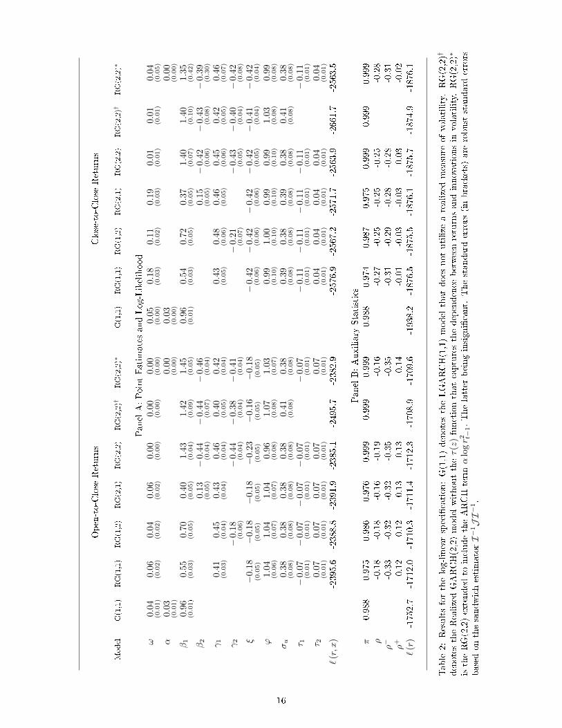
5.4.1 Log-Linear Models for SPY (Table 2)
Table 2 presents out empirical results for the log-linear speci�cation using six variants of the Realized GARCH
model. For the sake of comparison we use the logarithmic GARCH(1,1) model as the conventional benchmark,
when comparing the empirical �t in terms of the partial likelihood function (for returns). The left panel has
the empirical results for open-to-close SPY returns and the right panel has the corresponding results for
close-to-close SPY returns.
From Table 2 we see that the extended model RG(2, 2)∗, which includes the squared return in the GARCH
equation, results in very marginal improvements over the standard model RG(2, 2), and the ARCH parameter,
α, is clearly insigni�cant. Comparing the RG(2, 2)† with the standard model shows that the leverage function
is highly signi�cant. The improvement in the log-likelihood function is almost 100 units.
The robust standard errors suggest that β2 is signi�cant, when it is actually not the case. This is simply
a manifestation of a common problem with standard errors and t-statistics in the context with collinearity.
In this case, log ht−1 and log ht−2 are highly collinear which causes the likelihood surface to be almost �at
along lines where β1 + β2 is constant, while there is su�cient curvature along the axis to make the standard
errors small.
The estimates of ϕ are close to unity, ϕ ' 1, for both open-to-close and close-to-close returns. This
suggests that the realized measure, xt, is roughly proportional to the conditional variance for both open-
to-close returns and close-to-close returns. The fact that ξ is estimated to be smaller (more negative) for
close-to-close returns than for open-to-close returns simply re�ects that the realized measure is computed
over an interval that spans a shorter period than close-to-close returns.
In terms of partial log-likelihood function, `(r), the Realized GARCH models clearly dominate the con-
ventional logarithmic GARCH(1,1). The corresponding results for the Realized GARCH models based on a
linear speci�cation, are reported in a separate web appendix. These show that the log-linear speci�cation
dominates the linear speci�cation. In the RG(2, 2)∗ which includes log r2t−1 in the GARCH equation, we
replace about ten squared zero close-to-close returns by the truncation parameter ε. The standard errors in
this model are rather sensitive to the value of the truncation parameter. The problem disappears if we use
a smaller truncation parameter, but the smaller truncation parameter also causes the performance of the
15
Open-to-Close
Returns
Close-to-Close
Returns
Model
G(1,1)
RG(1,1)
RG(1,2)
RG(2,1)
RG(2,2)
RG(2,2)†
RG(2,2)∗
G(1,1)
RG(1,1)
RG(1,2)
RG(2,1)
RG(2,2)
RG(2,2)†
RG(2,2)∗
PanelA:PointEstimatesandLog-Likelihood
ω0.
04(0.01)
0.06
(0.02)
0.04
(0.02)
0.06
(0.02)
0.00
(0.00)
0.00
(0.00)
0.0
0(0.00)
0.05
(0.00)
0.1
8(0.03)
0.11
(0.02)
0.1
9(0.03)
0.01
(0.01)
0.01
(0.01)
0.04
(0.05)
α0.0
3(0.01)
0.0
0(0.00)
0.03
(0.00)
0.00
(0.00)
β1
0.96
(0.01)
0.55
(0.03)
0.7
0(0.05)
0.40
(0.05)
1.4
3(0.04)
1.42
(0.09)
1.4
5(0.05)
0.96
(0.01)
0.5
4(0.03)
0.72
(0.05)
0.3
7(0.05)
1.40
(0.07)
1.40
(0.10)
1.35
(0.42)
β2
0.13
(0.05)−
0.4
4(0.04)
−0.
44
(0.07)
−0.4
6(0.04)
0.1
5(0.05)−
0.42
(0.06)
−0.
43
(0.08)
−0.
39
(0.30)
γ1
0.41
(0.03)
0.4
5(0.04)
0.43
(0.04)
0.4
6(0.04)
0.40
(0.05)
0.4
2(0.04)
0.43
(0.05)
0.48
(0.06)
0.46
(0.05)
0.45
(0.06)
0.42
(0.05)
0.46
(0.07)
γ2
−0.1
8(0.06)
−0.4
4(0.04)
−0.3
8(0.04)
−0.4
1(0.04)
−0.
21
(0.07)
−0.
43
(0.05)
−0.
40
(0.04)
−0.
42
(0.08)
ξ−
0.18
(0.05)
−0.
18(0.05)
−0.
18(0.05)
−0.
23
(0.05)
−0.
16
(0.05)
−0.
18
(0.05)
−0.
42
(0.06)−
0.4
2(0.06)−
0.42
(0.06)−
0.4
2(0.05)
−0.
41
(0.04)
−0.4
2(0.04)
ϕ1.
04(0.06)
1.04
(0.07)
1.04
(0.07)
0.96
(0.08)
1.0
7(0.08)
1.03
(0.07)
0.99
(0.10)
1.0
0(0.10)
0.99
(0.10)
0.9
9(0.10)
1.03
(0.08)
0.9
9(0.08)
σu
0.3
8(0.08)
0.38
(0.08)
0.3
8(0.08)
0.38
(0.08)
0.4
1(0.08)
0.38
(0.08)
0.39
(0.08)
0.3
8(0.08)
0.39
(0.08)
0.3
8(0.08)
0.41
(0.08)
0.3
8(0.08)
τ 1−
0.0
7(0.01)−
0.07
(0.01)−
0.0
7(0.01)−
0.07
(0.01)
−0.
07
(0.01)
−0.
11
(0.01)−
0.1
1(0.01)−
0.11
(0.01)−
0.11
(0.01)
−0.1
1(0.01)
τ 20.0
7(0.01)
0.07
(0.01)
0.0
7(0.01)
0.07
(0.01)
0.07
(0.01)
0.04
(0.01)
0.04
(0.01)
0.04
(0.01)
0.04
(0.01)
0.04
(0.01)
`(r,x
)-2395.6
-2388.8
-2391.9
-2385.1
-2495.7
-2382.9
-2576.9
-2567.2
-2571.7
-2563.9
-2661.7
-2563.5
PanelB:Auxiliary
Statistics
π0.988
0.975
0.986
0.976
0.999
0.999
0.999
0.988
0.974
0.987
0.975
0.999
0.999
0.999
ρ-0.18
-0.18
-0.16
-0.19
-0.16
-0.27
-0.25
-0.25
-0.25
-0.28
ρ−
-0.33
-0.32
-0.32
-0.35
-0.35
-0.31
-0.29
-0.28
-0.28
-0.31
ρ+
0.12
0.12
0.13
0.13
0.14
-0.01
-0.03
-0.03
0.03
-0.02
`(r
)-1752.7
-1712.0
-1710.3
-1711.4
-1712.3
-1708.9
-1709.6
-1938.2
-1876.5
-1875.5
-1876.1
-1875.7
-1874.9
-1876.1
Table2:Resultsforthelog-linearspeci�cation:G(1,1)denotestheLGARCH(1,1)modelthatdoes
notutilize
arealizedmeasure
ofvolatility.RG(2,2)†
denotestheRealizedGARCH(2,2)modelwithouttheτ(z
)functionthatcapturesthedependence
betweenreturnsandinnovationsin
volatility.RG(2,2)∗
istheRG(2,2)extended
toincludetheARCH-termα
logr2 t−1.Thelatter
beinginsigni�cant.
Thestandard
errors
(inbrackets)
are
robust
standard
errors
basedonthesandwichestimatorI−
1JI−
1.
16
LGARCH to deteriorate substantially.
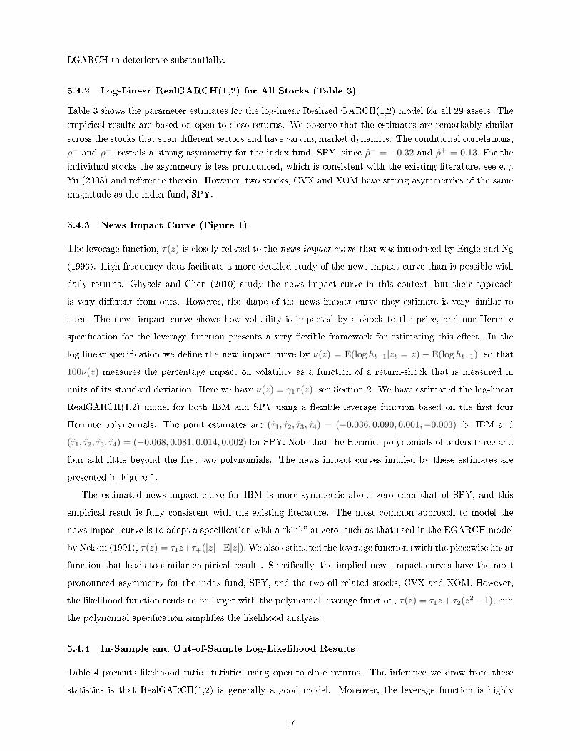
5.4.2 Log-Linear RealGARCH(1,2) for All Stocks (Table 3)
Table 3 shows the parameter estimates for the log-linear Realized GARCH(1,2) model for all 29 assets. The
empirical results are based on open-to-close returns. We observe that the estimates are remarkably similar
across the stocks that span di�erent sectors and have varying market dynamics. The conditional correlations,
ρ− and ρ+, reveals a strong asymmetry for the index fund, SPY, since ρ− = −0.32 and ρ+ = 0.13. For the
individual stocks the asymmetry is less pronounced, which is consistent with the existing literature, see e.g.
Yu (2008) and reference therein. However, two stocks, CVX and XOM have strong asymmetries of the same
magnitude as the index fund, SPY.
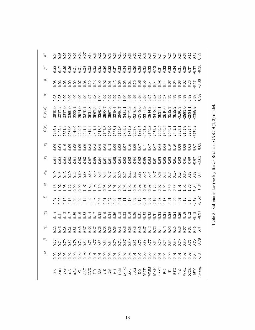
5.4.3 News Impact Curve (Figure 1)
The leverage function, τ(z) is closely related to the news impact curve that was introduced by Engle and Ng
(1993). High frequency data facilitate a more detailed study of the news impact curve than is possible with
daily returns. Ghysels and Chen (2010) study the news impact curve in this context, but their approach
is very di�erent from ours. However, the shape of the news impact curve they estimate is very similar to
ours. The news impact curve shows how volatility is impacted by a shock to the price, and our Hermite
speci�cation for the leverage function presents a very �exible framework for estimating this e�ect. In the
log-linear speci�cation we de�ne the new impact curve by ν(z) = E(log ht+1|zt = z) − E(log ht+1), so that
100ν(z) measures the percentage impact on volatility as a function of a return-shock that is measured in
units of its standard deviation. Here we have ν(z) = γ1τ(z), see Section 2. We have estimated the log-linear
RealGARCH(1,2) model for both IBM and SPY using a �exible leverage function based on the �rst four
Hermite polynomials. The point estimates are (τ1, τ2, τ3, τ4) = (−0.036, 0.090, 0.001,−0.003) for IBM and
(τ1, τ2, τ3, τ4) = (−0.068, 0.081, 0.014, 0.002) for SPY. Note that the Hermite polynomials of orders three and
four add little beyond the �rst two polynomials. The news impact curves implied by these estimates are
presented in Figure 1.
The estimated news impact curve for IBM is more symmetric about zero than that of SPY, and this
empirical result is fully consistent with the existing literature. The most common approach to model the
news impact curve is to adopt a speci�cation with a �kink� at zero, such as that used in the EGARCH model
by Nelson (1991), τ(z) = τ1z+τ+(|z|−E|z|).We also estimated the leverage functions with the piecewise linear
function that leads to similar empirical results. Speci�cally, the implied news impact curves have the most
pronounced asymmetry for the index fund, SPY, and the two oil related stocks, CVX and XOM. However,
the likelihood function tends to be larger with the polynomial leverage function, τ(z) = τ1z+ τ2(z2− 1), and
the polynomial speci�cation simpli�es the likelihood analysis.
5.4.4 In-Sample and Out-of-Sample Log-Likelihood Results
Table 4 presents likelihood ratio statistics using open-to-close returns. The inference we draw from these
statistics is that RealGARCH(1,2) is generally a good model. Moreover, the leverage function is highly
17
ωβ
γ1
γ2
ξϕ
σu
τ 1τ 2
`(r
)`
(r,x
)π
ρρ−
ρ+
AA
0.03
0.77
0.33
-0.14
-0.07
1.15
0.40
-0.04
0.09
-2776.4
-3519.9
0.98
-0.08
-0.32
0.24
AIG
0.02
0.74
0.45
-0.21
-0.06
1.02
0.45
-0.02
0.04
-2403.1
-3317.2
0.98
-0.06
-0.17
0.08
AXP
0.05
0.70
0.38
-0.12
-0.16
1.08
0.43
-0.02
0.10
-2371.1
-3217.9
0.99
-0.05
-0.30
0.25
BA
0.02
0.82
0.31
-0.17
-0.13
1.22
0.39
-0.03
0.09
-2536.0
-3260.0
0.99
-0.09
-0.36
0.26
BAC
0.00
0.78
0.51
-0.29
0.00
0.99
0.42
-0.04
0.08
-2016.9
-2823.4
0.99
-0.09
-0.31
0.21
C-0.02
0.74
0.45
-0.19
0.09
0.99
0.39
-0.03
0.09
-2260.5
-2974.0
0.99
-0.07
-0.31
0.24
CAT
0.03
0.82
0.37
-0.22
-0.14
1.07
0.38
-0.03
0.09
-2621.1
-3279.4
0.99
-0.08
-0.32
0.27
CVX
0.03
0.71
0.33
-0.14
-0.09
1.32
0.39
-0.08
0.08
-2319.1
-3021.8
0.97
-0.19
-0.35
0.14
DD
-0.01
0.77
0.37
-0.17
0.08
1.08
0.40
-0.05
0.08
-2301.2
-3067.3
0.98
-0.13
-0.35
0.20
DIS
0.01
0.85
0.39
-0.25
-0.05
1.10
0.41
-0.04
0.09
-2518.5
-3289.6
1.00
-0.09
-0.35
0.22
GE
0.00
0.81
0.38
-0.19
0.01
0.98
0.41
-0.01
0.08
-2197.8
-2988.7
0.99
-0.02
-0.26
0.25
GM
0.06
0.84
0.39
-0.24
-0.32
1.02
0.47
-0.01
0.12
-2987.9
-3967.3
0.99
-0.01
-0.33
0.31
HD
0.01
0.79
0.39
-0.20
0.00
1.01
0.41
-0.05
0.09
-2538.4
-3318.4
0.99
-0.13
-0.37
0.20
IBM
0.00
0.74
0.41
-0.15
0.01
0.94
0.39
-0.04
0.08
-2192.6
-2896.7
0.98
-0.09
-0.32
0.24
INTC
0.02
0.87
0.46
-0.33
-0.11
1.03
0.36
-0.02
0.07
-2869.1
-3481.1
1.00
-0.05
-0.24
0.22
JNJ
-0.03
0.80
0.38
-0.19
0.13
1.04
0.44
0.02
0.10
-1874.8
-2777.3
0.99
0.04
-0.25
0.30
JPM
0.01
0.81
0.49
-0.30
-0.02
0.98
0.42
-0.04
0.09
-2463.0
-3276.8
0.99
-0.10
-0.30
0.22
KO
-0.05
0.76
0.45
-0.21
0.19
0.93
0.38
-0.02
0.07
-1886.7
-2573.6
0.99
-0.06
-0.28
0.19
MCD
0.00
0.88
0.37
-0.25
-0.01
0.98
0.45
-0.05
0.11
-2461.8
-3371.9
0.99
-0.09
-0.35
0.26
MMM
0.00
0.77
0.43
-0.23
0.02
0.98
0.41
-0.02
0.07
-2140.3
-2944.8
0.97
-0.04
-0.23
0.21
MRK
0.03
0.84
0.33
-0.21
-0.19
1.23
0.47
0.01
0.07
-2479.2
-3478.5
0.98
0.04
-0.13
0.18
MSFT
-0.01
0.79
0.44
-0.22
0.08
0.92
0.38
-0.03
0.08
-2330.7
-3021.1
0.99
-0.08
-0.31
0.24
PG
-0.04
0.78
0.43
-0.25
0.18
1.04
0.41
-0.05
0.08
-1850.7
-2646.6
0.98
-0.14
-0.32
0.14
T0.00
0.86
0.53
-0.38
0.01
0.86
0.46
-0.03
0.10
-2560.4
-3512.7
0.99
-0.07
-0.32
0.25
UTX
-0.01
0.80
0.45
-0.24
0.06
0.88
0.40
-0.01
0.10
-2302.4
-3059.2
0.99
-0.05
-0.34
0.29
VZ
-0.01
0.79
0.40
-0.20
0.07
1.01
0.43
-0.03
0.09
-2343.4
-3196.7
0.99
-0.08
-0.31
0.23
WMT
-0.02
0.80
0.37
-0.19
0.12
1.04
0.39
-0.01
0.09
-2164.9
-2893.6
0.99
-0.02
-0.29
0.30
XOM
0.03
0.71
0.34
-0.12
-0.10
1.26
0.38
-0.08
0.08
-2334.7
-2994.1
0.98
-0.20
-0.37
0.15
SPY
0.04
0.70
0.45
-0.18
-0.18
1.04
0.38
-0.07
0.07
-1710.3
-2388.8
0.99
-0.17
-0.32
0.13
Average
0.01
0.79
0.41
-0.21
-0.02
1.04
0.41
-0.03
0.09
0.99
-0.08
-0.30
0.22
Table3:Estimatesforthelog-linearRealizedGARCH
(1,2
)model.
18
Figure 1: News impact curve for IBM and SPY
signi�cant while α is insigni�cant.
The statistics in Panel A are conventional likelihood ratio statistics,
LRi = 2{`RG(2,2)∗(r, x)− `i(r, x)
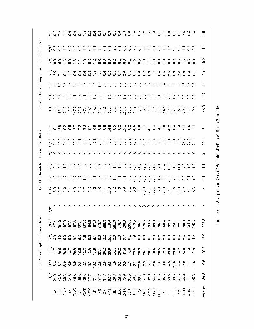
}, i = 1, . . . , 5,
where each of the �ve smaller models are benchmarked against the largest model. The largest model is the
log-linear RealGARCH(2,2) model that includes the squared returns in the GARCH equation (in addition
to the realized measure). In the QMLE framework the limit distribution of likelihood ratio statistic, LRi,
is usually given as a weighted sum of χ2-distributed random variables. So comparing the LRi to the usual
critical value of a χ2-distribution is only indicative of signi�cance. The LR statistics in the column labeled
�(2,2)� are small in most cases, so there is little evidence that α is signi�cant. This is consistent with
the existing literature, since squared returns are typically found to be insigni�cant once a realized measure
is included in the GARCH equation. The LR statistics in column �(2,2)†� are well over 100 in all cases.
This shows that the leverage function, τ(zt), is highly signi�cant. Similarly, the LR statistics shows that the
hypothesis, β2 = γ2 = 0, is rejected in most cases. So the empirical evidence does not support a simpli�cation
of the model to the RealGARCH(1,1). The results for the two sub-hypotheses, β2 = 0 and γ2 = 0, are less
conclusive. The likelihood ratio statistics for the hypothesis, β2 = 0 (which is given as the di�erence between
the statistics in columns �(1,2)� and �(2,2)�) are on average 5.7 = 9.6 − 3.9. In a correctly speci�ed model,
this would be borderline signi�cant. The LR statistics for the hypothesis, γ2 = 0, tend to be larger with an
average value of 16.6 = 20.5 − 3.9. So the empirical evidence favors the RealGARCH(1,2) model over the
RealGARCH(2,1) model.
The statistics in Panel B are out-of-sample likelihood ratio statistics, de�ned by√
nm{`RG(2,2)(r, x) −
19
`j(r, x)}, where n and m denote the sample sizes, in-sample and out-of-sample, respectively. The in-sample
estimates are simply plugged into the out-of-sample log-likelihood function. The asymptotic distribution of
the out-of-sample LR statistic is non-standard. However in a nested comparison where the larger model has
k additional parameters (that are all zero in population) it can be shows that
√n
m{`i(r, x)− `j(r, x)} d→ Z ′1ΛZ2, as m,n→∞ with m/n→ 0,
where Z1 and Z2 are independent Zi ∼ Nk(0, I), and Λ is a diagonal matrix with the eigenvalues from I−1J ,
see Hansen (2009). For correctly speci�ed models (Λ = I) the (two-sided) critical values can be inferred
from the distribution of |Z ′1Z2|. For k = 1 the 5% and 1% critical values are 2.25 and 3.67, respectively,
and for two degrees of freedom (k = 2), these are 3.05 and 4.83, respectively. While our model is likely
to be misspeci�ed to some degree, we will later argue that the log-linear Gaussian speci�cation is not very
misspeci�ed. So we will take these critical values as reasonably approximation. Compared to these critical
values we �nd, on average, signi�cant evidence in favor of a model with more lags than RealGARCH(1,1).
The statistical evidence in favor of a leverage function is again very strong. Adding the ARCH parameter, α,
will (on average) result in a worse out-of-sample log-likelihood. On average, we have a tie between the three
models: RealGARCH(1,2), RealGARCH(2,1), and RealGARCH(2,2).
In Panel C, we report partial out-of-sample likelihood ratio statistics that are de�ned by 2{maxi `i(r|x)−
`j(r|x)}. This LR statistics are based on the partial likelihood for returns, which enables us to compare
the empirical �t to the conventional LGARCH. Again we see that the Realized GARCH models strongly
dominate the LGARCH(1,1) model. This is impressive because the Realized GARCH models are not seeking
to maximize the partial likelihood, as is the objective for the LGARCH model.4
5.5 A Comparison of the Linear and Log-Linear Speci�cations
One of the reasons we prefer the log-linear Gaussian speci�cation over the linear Gaussian speci�cation
is because the former is much less at odds with data. The log-linear speci�cation results in far less het-
eroskedasticity, as is evident from Figure 2. The left panel is a scatter plot of xt against ht, (for the linear
RealGARCH(1,2) model) and the right panel is a scatter plot of log xt against log ht (for the log-linear
RealGARCH(1,2) model). The two models produce very similar value for ht, however there is obviously a
very pronounced degree of heteroskedasticity in the linear models. The linear model may be improved by
modifying the leverage function, but our point is that the simple measurement equation does a good job
within the log-linear speci�cation. Homoskedastic errors are not essential for the quasi maximum likelihood
estimators but heteroskedasticity causes the QMLE to be ine�cient. Moreover, misspeci�cation causes the
likelihood ratio statistic to have an asymptotic distribution that is a weighted sum of χ2(1)-distributed ran-
dom variables, rather than a pure sum of such. Comparing likelihood ratio statistics to critical values to a
4The asymptotic distribution of these statistics is very non-standard (and generally unknown) because we are comparinga model that maximizes the partial likelihood (the LGARCH(1,1) model) with models that maximize a joint likelihood (theRealized GARCH models).
20
PanelA:In-Sample
LikelihoodRatio
PanelB:Out-of-Sample
LikelihoodRatio
PanelC:Out-of-Sample
PartialLikelihoodRatio
(1,1)
(1,2)
(2,1)
(2,2)
(2,2)†
(2,2)∗
(1,1)
(1,2)
(2,1)
(2,2)
(2,2)†
(2,2)∗
G11
(1,1)
(1,2)
(2,1)
(2,2)
(2,2)†
(2,2)∗
AA
24.0
8.3
11.7
3.9
187.4
06.9
4.5
6.4
021.9
0.1
4.6
3.3
1.4
2.6
0.0
0.6
0.7
AIG
43.8
15.2
20.6
14.2
201.2
015.7
-0.2
6.0
025.5
12.5
56.1
9.3
5.9
7.4
6.0
0.0
7.2
AXP
30.5
25.0
26.0
0.0
197.0
01.2
2.7
1.5
013.3
0.2
24.0
0.0
0.3
0.1
1.3
1.7
1.4
BA
34.8
6.0
18.8
0.0
197.1
0-1.4
0.4
-2.6
024.5
0.0
1.1
0.6
1.8
1.7
0.0
0.3
0.0
BAC
46.3
5.9
20.5
5.1
198.8
08.0
-0.7
-0.3
056.5
-2.8
147.9
4.1
0.6
0.0
1.5
19.7
0.9
C26.8
9.5
16.0
6.3
228.4
01.3
-2.7
-2.5
0-0.1
-7.2
26.9
0.3
0.9
0.5
1.1
0.0
0.4
CAT
39.8
2.3
13.8
1.6
227.3
01.7
-1.0
-4.2
09.0
2.2
47.3
0.1
0.8
0.0
1.0
1.6
1.5
CVX
17.7
0.1
3.5
0.0
194.6
05.3
0.0
2.2
020.8
-0.1
30.1
0.6
0.3
0.2
0.3
0.0
0.3
DD
31.1
10.8
15.9
6.1
167.0
04.6
4.1
3.0
0-7.1
6.9
19.2
1.2
1.5
1.5
1.2
1.4
0.0
DIS
57.7
12.6
33.1
0.0
213.7
04.8
4.8
3.7
024.3
0.0
35.4
0.0
2.0
1.4
0.8
1.1
0.8
GE
37.7
12.6
20.2
12.2
200.3
014.1
0.6
5.9
09.3
0.6
41.6
0.9
0.0
0.6
0.0
0.3
0.7
GM
62.7
18.8
39.9
18.4
319.9
017.0
-0.2
6.8
07.2
14.6
57.5
1.4
0.0
0.2
0.0
0.3
0.9
HD
29.8
4.0
14.4
2.0
201.3
02.2
-1.0
-1.0
028.9
0.5
45.5
0.9
0.0
0.1
0.2
2.1
0.4
IBM
28.5
16.2
20.2
1.0
176.7
03.3
-0.1
1.0
025.0
-0.2
12.0
0.4
0.5
0.7
0.1
0.3
0.0
INTC
75.9
13.9
47.8
9.7
130.8
00.9
0.1
-3.4
036.8
19.1
133.1
1.7
0.5
2.0
0.0
0.1
1.8
JNJ
34.6
1.3
4.8
0.1
235.4
07.1
-0.8
2.0
030.7
0.2
21.8
0.4
0.0
0.1
0.1
0.1
0.0
JPM
50.7
3.5
23.6
1.9
213.5
00.3
-2.5
-5.4
0-3.6
-0.6
34.9
0.0
1.3
0.1
1.6
2.0
1.6
KO
39.7
22.0
28.3
0.0
186.1
02.1
-2.8
-1.0
022.6
0.0
5.6
0.4
0.6
0.0
0.5
0.9
0.5
MCD
54.8
2.9
26.1
0.8
278.6
0-13.0
-0.6
-9.3
047.4
1.4
6.8
0.0
1.5
0.2
1.8
2.0
1.7
MMM
32.0
6.7
20.4
0.1
183.5
0-2.4
-0.2
-2.8
024.5
-0.1
14.5
0.0
1.9
0.9
1.4
1.0
1.4
MRK
64.6
12.0
10.6
2.9
309.0
0-3.4
-2.5
-1.2
032.4
0.4
11.8
0.0
1.6
1.7
1.9
2.4
1.8
MSFT
37.3
11.5
20.5
10.2
186.1
08.3
4.2
7.1
017.0
4.1
37.1
0.1
0.5
0.4
0.0
0.2
0.1
PG
36.5
3.0
12.3
2.9
160.4
0-1.3
0.3
-0.4
035.0
1.0
24.8
0.0
1.4
0.6
1.3
1.5
1.7
T69.8
4.8
39.0
0.0
198.3
019.7
-0.3
13.5
035.1
-0.2
19.2
2.8
0.2
2.6
0.0
1.7
0.0
UTX
39.6
21.6
29.0
0.0
223.7
05.8
-2.0
1.2
033.1
-0.4
12.3
1.4
0.2
0.9
0.2
0.0
0.1
VZ
31.5
4.3
13.2
0.5
188.7
015.0
3.2
11.1
016.6
-1.3
8.7
3.5
0.7
2.8
0.3
0.0
0.1
WMT
36.2
12.0
23.0
8.3
190.0
0-7.2
-3.8
-7.9
028.7
9.4
30.5
0.0
0.6
0.0
1.3
1.4
2.6
XOM
14.7
1.1
4.3
0.9
234.0
05.7
-0.1
1.0
027.9
0.6
21.6
0.0
0.5
0.3
0.5
0.5
0.5
SPY
25.3
11.6
17.9
4.2
225.6
06.3
-1.2
1.9
024.4
1.4
40.8
0.8
0.6
0.7
0.0
2.5
1.3
Average
39.8
9.6
20.5
3.9
208.8
04.4
0.1
1.1
023.0
2.1
33.5
1.2
1.0
1.0
0.8
1.6
1.0
Table4:In-SampleandOut-of-SampleLikelihoodRatioStatistics
21
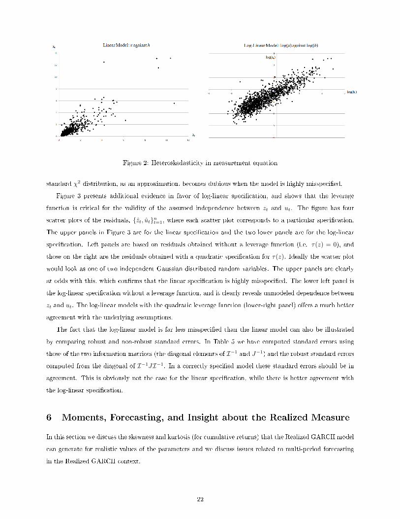
Figure 2: Heteroskedasticity in measurement equation
standard χ2-distribution, as an approximation, becomes dubious when the model is highly misspeci�ed.
Figure 3 presents additional evidence in favor of log-linear speci�cation, and shows that the leverage
function is critical for the validity of the assumed independence between zt and ut. The �gure has four
scatter plots of the residuals, {zt, ut}nt=1, where each scatter plot corresponds to a particular speci�cation.
The upper panels in Figure 3 are for the linear speci�cation and the two lower panels are for the log-linear
speci�cation. Left panels are based on residuals obtained without a leverage function (i.e. τ(z) = 0), and
those on the right are the residuals obtained with a quadratic speci�cation for τ(z). Ideally the scatter plot
would look as one of two independent Gaussian distributed random variables. The upper panels are clearly
at odds with this, which con�rms that the linear speci�cation is highly misspeci�ed. The lower-left panel is
the log-linear speci�cation without a leverage function, and it clearly reveals unmodeled dependence between
zt and ut. The log-linear models with the quadratic leverage function (lower-right panel) o�ers a much better
agreement with the underlying assumptions.
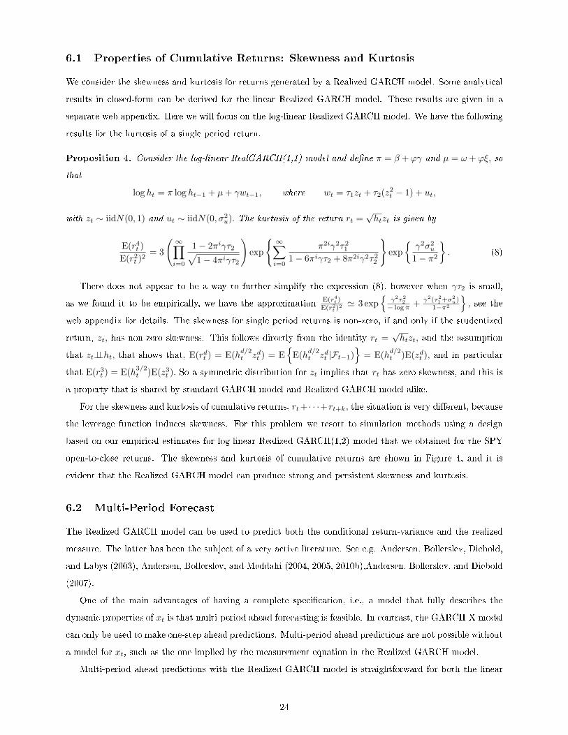
The fact that the log-linear model is far less misspeci�ed than the linear model can also be illustrated
by comparing robust and non-robust standard errors. In Table 5 we have computed standard errors using
those of the two information matrices (the diagonal elements of I−1 and J−1) and the robust standard errors
computed from the diagonal of I−1JI−1. In a correctly speci�ed model these standard errors should be in
agreement. This is obviously not the case for the linear speci�cation, while there is better agreement with
the log-linear speci�cation.
6 Moments, Forecasting, and Insight about the Realized Measure
In this section we discuss the skewness and kurtosis (for cumulative returns) that the Realized GARCH model
can generate for realistic values of the parameters and we discuss issues related to multi-period forecasting
in the Realized GARCH context.
22
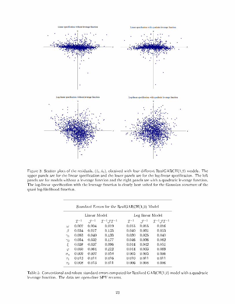
Figure 3: Scatter plots of the residuals, (zt, ut), obtained with four di�erent RealGARCH(1,2) models. Theupper panels are for the linear speci�cation and the lower panels are for the log-linear speci�cation. The leftpanels are for models without a leverage function and the right panels are with a quadratic leverage function.The log-linear speci�cation with the leverage function is clearly best suited for the Gaussian structure of thequasi log-likelihood function.
Standard Errors for the RealGARCH(1,2) Model
Linear Model Log-linear Model
I−1 J−1 I−1J I−1 I−1 J−1 I−1J I−1ω 0.007 0.004 0.019 0.015 0.015 0.016β 0.034 0.017 0.125 0.040 0.031 0.053γ1 0.053 0.040 0.133 0.030 0.025 0.040γ2 0.054 0.032 0.177 0.046 0.036 0.062ξ 0.038 0.037 0.096 0.044 0.042 0.051ϕ 0.080 0.064 0.212 0.044 0.033 0.069σu 0.009 0.002 0.054 0.005 0.005 0.006τ1 0.013 0.014 0.016 0.010 0.011 0.011τ2 0.008 0.013 0.011 0.006 0.008 0.006
Table 5: Conventional and robust standard errors computed for Realized GARCH(1,2) model with a quadraticleverage function. The data are open-close SPY returns.
23
6.1 Properties of Cumulative Returns: Skewness and Kurtosis
We consider the skewness and kurtosis for returns generated by a Realized GARCH model. Some analytical
results in closed-form can be derived for the linear Realized GARCH model. These results are given in a
separate web appendix. Here we will focus on the log-linear Realized GARCH model. We have the following
results for the kurtosis of a single period return.
Proposition 4. Consider the log-linear RealGARCH(1,1) model and de�ne π = β + ϕγ and µ = ω + ϕξ, so
that
log ht = π log ht−1 + µ+ γwt−1, where wt = τ1zt + τ2(z2t − 1) + ut,
with zt ∼ iidN(0, 1) and ut ∼ iidN(0, σ2u). The kurtosis of the return rt =
√htzt is given by
E(r4t )
E(r2t )2
= 3
( ∞∏i=0
1− 2πiγτ2√1− 4πiγτ2
)exp
{ ∞∑i=0
π2iγ2τ211− 6πiγτ2 + 8π2iγ2τ22
}exp
{γ2σ2
u
1− π2
}. (8)
There does not appear to be a way to further simplify the expression (8), however when γτ2 is small,
as we found it to be empirically, we have the approximationE(r4t )
E(r2t )2 ' 3 exp
{γ2τ2
2
− log π +γ2(τ2
1+σ2u)
1−π2
}, see the
web appendix for details. The skewness for single period returns is non-zero, if and only if the studentized
return, zt, has non-zero skewness. This follows directly from the identity rt =√htzt, and the assumption
that zt⊥⊥ht, that shows that, E(rdt ) = E(hd/2t zdt ) = E
{E(h
d/2t zdt |Ft−1)
}= E(h
d/2t )E(zdt ), and in particular
that E(r3t ) = E(h3/2t )E(z3t ). So a symmetric distribution for zt implies that rt has zero skewness, and this is
a property that is shared by standard GARCH model and Realized GARCH model alike.
For the skewness and kurtosis of cumulative returns, rt+ · · ·+rt+k, the situation is very di�erent, because
the leverage function induces skewness. For this problem we resort to simulation methods using a design
based on our empirical estimates for log-linear Realized GARCH(1,2) model that we obtained for the SPY
open-to-close returns. The skewness and kurtosis of cumulative returns are shown in Figure 4, and it is
evident that the Realized GARCH model can produce strong and persistent skewness and kurtosis.
6.2 Multi-Period Forecast
The Realized GARCH model can be used to predict both the conditional return-variance and the realized
measure. The latter has been the subject of a very active literature. See e.g. Andersen, Bollerslev, Diebold,
and Labys (2003), Andersen, Bollerslev, and Meddahi (2004, 2005, 2010b),Andersen, Bollerslev, and Diebold
(2007).
One of the main advantages of having a complete speci�cation, i.e., a model that fully describes the
dynamic properties of xt is that multi-period ahead forecasting is feasible. In contrast, the GARCH-X model
can only be used to make one-step ahead predictions. Multi-period ahead predictions are not possible without
a model for xt, such as the one implied by the measurement equation in the Realized GARCH model.
Multi-period ahead predictions with the Realized GARCH model is straightforward for both the linear
24
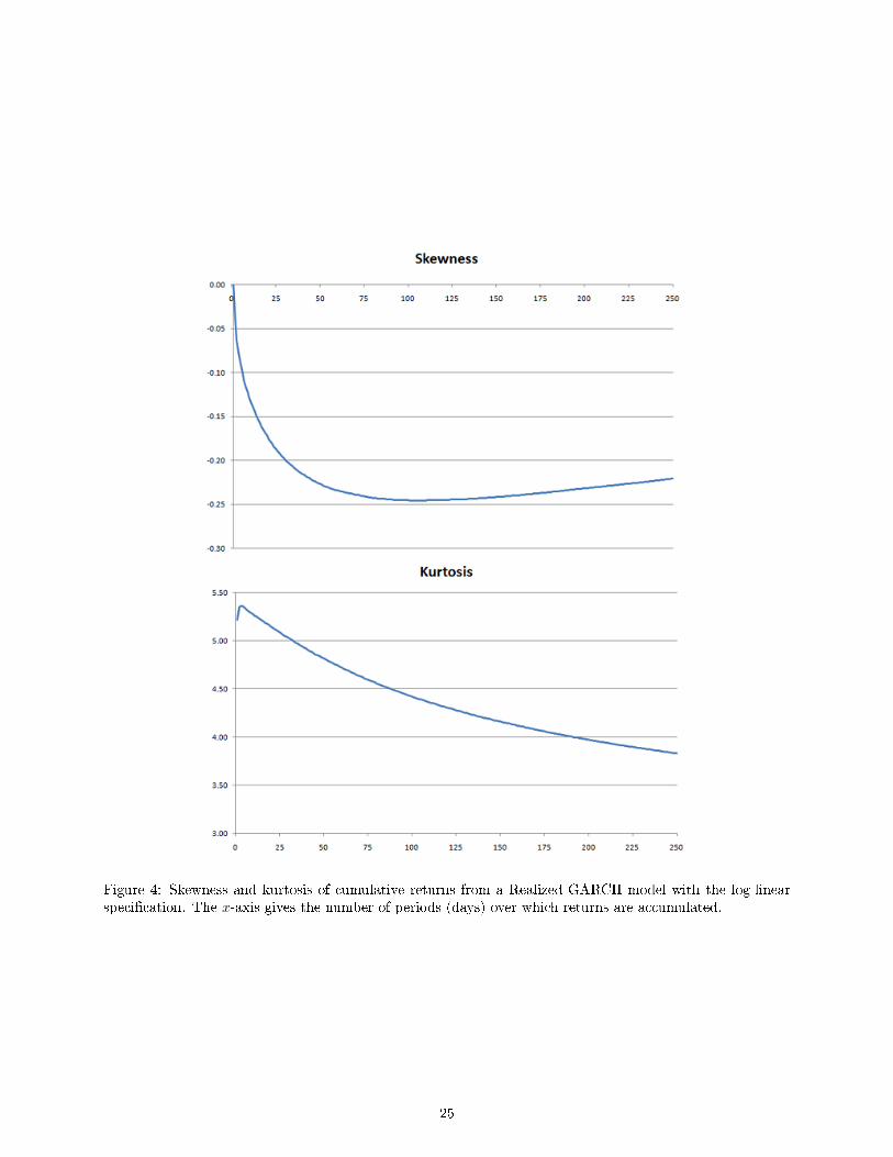
Figure 4: Skewness and kurtosis of cumulative returns from a Realized GARCH model with the log-linearspeci�cation. The x-axis gives the number of periods (days) over which returns are accumulated.
25
and log-linear Realized GARCH models. Let ht denote either ht or log ht, and consider �rst the case where
p = q = 1. By substituting the GARCH equation into measurement equation we obtain the VARMA(1,1)
structure ht
xt
=
β γ
ϕβ ϕγ
ht−1
xt−1
+
ω
ξ + ϕω
+
0
τ(zt) + ut
,that can be used to generate the predictive distribution of future values of ht, xt, as well as returns rt, using
ht+k
xt+k
=
β γ
ϕβ ϕγ
h ht
xt
+
k−1∑j=0
β γ
ϕβ ϕγ
j ω
ξ + ϕω
+
0
τ(zt+h−j) + ut+h−j
.
This is easily extended to the general case (p, q ≥ 1) where we have Yt = AYt−1 + b+ εt, with the conventions
Yt =
ht
.
.
.
ht−p+1
xt
.
.
.
xt−q+1
, A =
(β1, . . . , βp) (γ1, . . . , γq)
(Ip−1×p−1, 0p−1×1) 0p−1×q
ϕ(β1, . . . , βp) ϕ(γ1, . . . , γq)
0q−1×p (Iq−1×q−1, 0q−1×1)
, b =
ω
0p−1×1
ξ + ϕω
0q−1×1
, εt =
0p×1
τ(zt) + ut
0q×1
,
so that Yt+k = AkYt +∑k−1j=0 A
j(b+ εt+k−j). The predictive distribution for ht+h and/or xt+h, is given from
the distribution of∑k−1i=0 A
iεt+h−i, which also enables us to compute a predictive distribution for rt+k, and
cumulative returns rt+1 + · · · + rt+k. An advantage of the linear speci�cation is that it directly produces
a point forecast of future volatility, (ht+1, . . . , ht+k). With the log-linear speci�cation one would have to
account for distributional aspects of log ht+k, in order to produce an unbiased forecast of ht+k. This should
not be a major obstacle because the log-linear Gaussian speci�cation appears to work well with these data.
Note that one is not required to generate axillary future values of the realized measure, when the objective
is to predict future values of ht or the distribution of future (cumulative) returns. The reason is that the
innovations, zt and ut, are su�cient for generating the volatility path (and returns).
7 Conclusion
In this paper we have proposed a complete model for returns and realized measures of volatility, xt, where the
latter is tied directly to the conditional volatility ht. We have demonstrated that the model is straightforward
to estimate and o�ers a substantial improvement in the empirical �t, relative to standard GARCH models
based on daily returns only. The model is informative about realized measurement, such as its accuracy.
Our empirical analysis can be extended in a number of ways. For instance, inclusion of a jump robust
realized measure would be an interesting extension, because Andersen et al. (2007) have shown that the
predictability in volatility is largely driven by the continuous component of volatility. Moreover, Bollerslev,
Kretschmer, Pigorsch, and Tauchen (2009) have found that the leverage e�ect primarily acts through the
26

continuous volatility component. Another possible extension is to introduce a bivariate model of open-to-close
and close-to-open returns, as an alternative to modeling close-to-close returns, see Andersen et al. (2010a).
The Realized GARCH framework is naturally extended to a multi-factor structure. Say m realized
measures and k latent volatility variables. The Realized GARCH model discussed in this paper corresponds
to the case k = 1, whereas the MEM framework corresponds to the case m = k. Such a hybrid framework
would enable us to conduct inference about the number of latent factors, k. We could, in particular, test the
one-factor structure used in this paper, against the multi-factor structure implied by MEM.
A Appendix of Proofs
Proof of Proposition 1. The �rst result follows by substituting log xt = ϕ log ht+ ξ+wt and log r2t = log ht+κ+ vt into the
GARCH equation and rearranging. Next, we substitute log ht = (log xt − ξ −wt)/ϕ, log r2t = (log xt − ξ −wt)/ϕ+ κ+ vt, and
multiply by ϕ, and �nd
log xt − ξ − wt = ϕω +∑p∨q
i=1(βi + αi)(log xt−i − ξ − wt−i) + ϕ
∑q
j=1γj log xt−j + ϕ
∑q
j=1αj(κ+ vt−j)
so with πi = αi + βi + γiϕ we have
log xt = ξ(1− β• − α•) + ϕκα• + ϕω +
p∨q∑i=1
πi log xt−i + wt −∑p
i=1(αi + βi)wt−i + ϕ
∑q
j=1αjvt−j .
When ϕ = 0 the measurement equation shows that log xt is an iid process. �
Proof of Lemma 1. First note that∂g′t∂λ
=(0, ht−1, . . . , ht−p, 0p+q+1×q
)=: Ht−1. Thus from the GARCH equation,
ht = λ′gt, we have that ht =∂g′t∂λ
λ+ gt = Ht−1λ+ gt =∑pi=1 βiht−i + gt. Similarly, the second order derivative, is given by
ht =∂(gt + Ht−1λ)
∂λ′=∂gt
∂λ′+ Ht−1 +
Ht−1
∂λ′λ = H′t−1 + Ht−1 +
p∑i=1
βi∂ht−i
∂λ′=
p∑i=1
βiht−i + H′t−1 + Ht−1.
For the starting values we observe the following: Regardless of (h0, . . . , hp−1) being treated as �xed or as a vector of unknown
parameters, we have hs = hs = 0. Given the structure of ht this implies h1 = 0. When p = q = 1 it follows immediately
that ht =∑t−1j=0 β
jgt−j . Similarly we have ht =∑t−1j=0 β
j(Ht−1−j + Ht−1−j) =∑t−2j=0 β
j(Ht−1−j + Ht−1−j), where Ht =
(03×1, ht, 03×1) and where the second equality follows by H0 = 0. The result now follows from
t−2∑i=0
βiht−1−i =t−2∑i=0
βit−1−i−1∑j=0
βjgt−1−i−j =
t−2∑i=0
βit−i−2∑
k−i−1=0
βk−i−1gt−k =
t−2∑i=0
t−1∑k=i+1
βk−1gt−k =
t−1∑k=1
kβk−1gt−k.
�
Proof of Proposition 2. Recall that ut = xt − ψ′mt and ht= g′tλ. So the derivatives with respect to ht are given by
∂zt
∂ht=
∂rt exp(− 12ht)
∂ht= −
1
2zt so that
∂z2t∂ht
= −z2t ,
ut =∂ut
∂ht= −ϕ+
1
2ztτ′at, and ut =
∂ut
∂ht=∂(−ϕ+ 1
2zta(zt)′τ
)∂ht
= −1
4τ ′(ztat + z2t at
).
So with `t = − 12{ht + z2t + log(σ2
u) + u2t /σ2u} we have
∂`t
∂ut= 2
ut
σ2u
and∂`t
∂ht= −
1
2
{1 +
∂z2t∂ht
+∂u2t /∂ht
σ2u
}= −
1
2
{1− z2t +
2utut
σ2u
}.
Derivatives with respect to λ are ∂zt∂λ
= ∂zt∂ht
∂ht∂λ
= − 12ztht,
∂ut∂λ
= ∂ut∂ht
∂ht∂λ
= utht,∂ut∂λ′ = uth′t, and
∂`t∂λ
= ∂`t∂ht
ht =
− 12
{1− z2t + 2utut
σ2u
}ht. Derivatives with respect to ψ are ∂ut
∂ξ= −1, ∂ut
∂ξ= 0, ∂`t
∂ξ= ∂`t
∂ut
∂ut∂ξ
= −2 utσ2u, ∂ut∂ϕ
= −ht, ∂ut∂ϕ= −1,
27
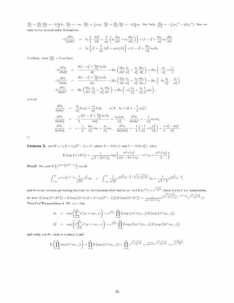
∂`t∂ϕ
= ∂`t∂ut
∂ut∂ϕ
= −2 utσ2uht,
∂ut∂τ
= −at, ∂ut∂τ = 12ztat,
∂`t∂τ
= ∂`t∂ut
∂ut∂τ
= −2 utσ2uat. Similarly,
∂`t∂σ2u
= − 12(σ−2u − u2tσ
−4u ). Now we
turn to the second order derivatives.
−2∂2`t
∂λ∂λ′= ht
{−∂z2t∂λ′
+2
σ2u
(ut∂ut
∂λ′+ ut
∂ut
∂λ′
)}+ (1− z2t +
2ut
σ2u
ut)∂ht
∂λ′
= ht
{z2t +
2
σ2u
(u2t + utut
)h′t
}+ (1− z2t +
2ut
σ2u
ut)ht.
Similarly, since ∂zt∂ψ
= 0 we have
−2∂2`t
∂λ∂ξ=
∂(1− z2t + 2utσ2uut)ht
∂ξ= 2ht
(∂ut
∂ψ′ut
σ2u
+ut
σ2u
∂ut
∂ξ
)= 2ht
(−ut
σ2u
+ 0
)
−2∂2`t
∂λ∂ϕ=
∂(1− z2t + 2utσ2uut)ht
∂ϕ= 2ht
(∂ut
∂ϕ
ut
σ2u
+ut
σ2u
∂ut
∂ϕ
)= 2ht
(−ht
ut
σ2u
−ut
σ2u
)−2
∂2`t
∂λ∂τ ′= 2ht
(∂ut
∂τ ′ut
σ2u
+ut
σ2u
∂ut
∂τ ′
)= 2ht
(−a′t
ut
σ2u
+ut
σ2u
1
2ztat
),
so that
∂2`t
∂λ∂ψ′=
ut
σ2u
htm′t +
ut
σ2u
htb′t, with bt = (0, 1,−
1
2zta′t)′,
∂2`t
∂λ∂σ2u
= −1
2
∂(1− z2t + 2utσ2uut)ht
∂σ2u
=ututht
σ4u
,∂2`t
∂ψ∂ψ′= −
1
σ2u
mtm′t,
∂2`t
∂ψ∂σ2u
= = −1
2(−
2ut
σ4u
)mt =ut
σ4u
mt,∂2`t
∂σ2u∂σ
2u
= −1
2
(−1σ4u
+ 2u2tσ6u
)=
1
2
σ2u − 2u2tσ6u
.
�
Lemma 2. Let W = τ1Z + τ2(Z2 − 1) + U, where Z ∼ N(0, 1) and U ∼ N(0, σ2u). Then
E(exp
{πiγW
})=
1√1− 2πiγτ2
exp
{π2iγ2τ21
2(1− 2πiγτ2)− πiγτ2 +
π2iγ2σ2u
2
}.
Proof . We have E(eaZ+ b
2(Z2−1)
)equals
ˆ ∞−∞
eaz+b2(z2−1) 1
√2πez2
2 dz =
ˆ ∞−∞
1√2πe
a2
2(1−b)−b2− 1
2
(z− a
1−b)
(1−b)−1 )dz =
1√1− b
ea2
2(1−b)−b2 ,
and from the moment generating function for the Gaussian distribution we have E(ecU
)= e
c2σ2u2 . Since Z and U are independent,
we have E(exp
{πiγW
})= E
(exp
{πiγτ1Z + πiγτ2(Z2 − 1)
})E(exp
{πiγU
})= 1√
1−2πiγτ2e
π2iγ2τ212(1−2πiγτ2)
−πiγτ2eπ2iγ2σ2u
2 .�
Proof of Proposition 4. We note that
ht = exp
( ∞∑i=0
πi(µ+ γwt−1)
)= e
µ1−π
∞∏i=0
Eexp(γπiτ(zt−i)
)E(exp
{πiγut−i
}),
h2t = exp
(2
∞∑i=0
πi(µ+ γwt−1)
)= e
2µ1−π
∞∏i=0
Eexp(2γπiτ(zt−i)
)E(exp
{2πiγut−i
}),
and using results, such as Lemma 2 and
E
( ∞∏i=0
exp{πiγut−i
})=
∞∏i=0
E(exp
{πiγut−i
})=∞∏i=0
eπ2iγ2σ2u
2 = e∑∞i=0
π2iγ2σ2u2 = e
γ2σ2u/2
1−π2 ,
28
we �nd thatEh2t
(Eht)2=
e2µ
1−π ∏∞i=0 E exp(2γπiwt−1)
e2µ
1−π ∏∞i=0{E exp(γπiwt−1)}2
equals
( ∞∏i=0
1− 2πiγτ2√1− 4πiγτ2
)e
∑∞i=0
4π2iγ2τ212(1−4πiγτ2)
e2∑∞i=0
π2iγ2τ212(1−2πiγτ2)
e− 2γτ2
1−π
e−2
γτ21−π
e2γ2σ2u1−π2
eγ2σ2u1−π2
=
( ∞∏i=0
1− 2πiγτ2√1− 4πiγτ2
)e
∑∞i=0
2π2iγ2τ21(1−4πiγτ2)
−π2iγ2τ21
(1−2πiγτ2) eγ2σ2u1−π2
=
( ∞∏i=0
1− 2πiγτ2√1− 4πiγτ2
)e
∑∞i=0
π2iγ2τ21(1−6πiγτ2+8π2iγ2τ22 ) e
γ2σ2u1−π2
where the last equality uses that2π2iγ2τ21
(1−4πiγτ2)− π2iγ2τ21
(1−2πiγτ2)equals
2π2iγ2τ21 (1− 2πiγτ2)− π2iγ2τ21 (1− 4πiγτ2)
(1− 4πiγτ2)(1− 2πiγτ2)=
π2iγ2τ21(1− 4πiγτ2)(1− 2πiγτ2)
=π2iγ2τ21
(1− 6πiγτ2 + 8π2iγ2τ22 ).
�
References
Andersen, T., Bollerslev, T., Diebold, F. X., 2007. Roughing it up: Including jump components in the measurement, modelingand forecasting of return volatility. Review of Economics and Statistics 89, 701�720.
Andersen, T., Dobrev, D., Schaumburg, E., 2008. Duration-based volatility estimation. working paper.
Andersen, T. G., Bollerslev, T., 1998. Answering the skeptics: Yes, standard volatility models do provide accurate forecasts.International Economic Review 39 (4), 885�905.
Andersen, T. G., Bollerslev, T., Diebold, F. X., Labys, P., 2001. The distribution of exchange rate volatility. Journal of theAmerican Statistical Association 96 (453), 42�55, correction published in 2003, volume 98, page 501.
Andersen, T. G., Bollerslev, T., Diebold, F. X., Labys, P., 2003. Modeling and forecasting realized volatility. Econometrica71 (2), 579�625.
Andersen, T. G., Bollerslev, T., Huang, X., 2010a. A reduced form framework for modeling volatility of speculative prices basedon realized variation measures. Forthcoming in Jounal of Econometrics.
Andersen, T. G., Bollerslev, T., Meddahi, N., 2004. Analytic evaluation of volatility forecasts. International Economic Review45, 1079�1110.
Andersen, T. G., Bollerslev, T., Meddahi, N., 2005. Correcting the errors: Volatility forecast evaluation using high-frequencydata and realized volatilities. Econometrica 73, 279�296.
Andersen, T. G., Bollerslev, T., Meddahi, N., 2010b. Market microstructure noise and realized volatility forecasting. Journal ofEconometrics.
Barndor�-Nielsen, O. E., Hansen, P. R., Lunde, A., Shephard, N., 2008. Designing realised kernels to measure the ex-postvariation of equity prices in the presence of noise. Econometrica 76, 1481�536.
Barndor�-Nielsen, O. E., Hansen, P. R., Lunde, A., Shephard, N., 2009a. Realised kernels in practice: Trades and quotes.Econometrics Journal 12, 1�33.
Barndor�-Nielsen, O. E., Hansen, P. R., Lunde, A., Shephard, N., 2010. Multivariate realised kernels: consistent positivesemi-de�nite estimators of the covariation of equity prices with noise and non-synchronous trading. Jounal of Econometricsforthcoming.
Barndor�-Nielsen, O. E., Kinnebrock, S., Shephard, N., 2009b. Measuring downside risk - realised semivariance. In: Watson,M. W., Bollerslev, T., Russell, J. (Eds.), Volatility and Time Series Econometrics: Essays in Honor of Robert Engle. OxfordUniversity Press.
Barndor�-Nielsen, O. E., Shephard, N., 2002. Econometric analysis of realised volatility and its use in estimating stochasticvolatility models. Journal of the Royal Statistical Society B 64, 253�280.
Barndor�-Nielsen, O. E., Shephard, N., 2004. Power and bipower variation with stochastic volatility and jumps (with discussion).Journal of Financial Econometrics 2, 1�48.
Barndor�-Nielsen, O. E., Shephard, N., 2007. Advances in Economics and Econometrics. Theory and Applications, Ninth WorldCongress. Econometric Society Monographs. Cambridge University Press, Ch. Variation, jumps and high frequency data in�nancial econometrics, pp. 328�372.
29
Bollerslev, T., 1986. Generalized autoregressive heteroskedasticity. Journal of Econometrics 31, 307�327.
Bollerslev, T., 2009. Glossary to ARCH (GARCH). In: Bollerslev, T., Russell, J. R., Watson, M. (Eds.), Volatility and TimeSeries Econometrics: Essays in Honour of Robert F. Engle. Oxford University Press, Oxford, UK.
Bollerslev, T., Kretschmer, U., Pigorsch, C., Tauchen, G., 2009. A discrete-time model for daily s&p500 returns and realizedvariations: Jumps and leverage e�ects. Journal of Econometrics 150, 151�166.
Bollerslev, T., Wooldridge, J. M., 1992. Quasi-maximum likelihood estimation and inference in dynamic models with time-varyingcovariance. Econometric Reviews 11, 143�172.
Brownless, C. T., Gallo, G. M., 2010. Comparison of volatility measures: A risk management perspective. Journal of FinancialEconometrics 8, 29�56.
Carrasco, M., Chen, X., 2002. Mixing and moment properties of various GARCH and stochastic volatility models. EconometricTheory 18, 17�39.
Chen, X., Ghysels, E., Wang, F., 2009. The HYBRID GARCH class of models. working paper.
Christo�ersen, P., Feunou, B., Jacobs, K., Meddahi, N., 2010. The economic value of realized volatility. working paper.
Cipollini, F., Engle, R. F., Gallo, G. M., 2009. A model for multivariate non-negative valued processes in �nancial econometrics.working paper.
Dobrev, D., Szerszen, P., 2010. The information content of high-frequency data for estimating equity return models and fore-casting risk. working paper.
Engle, R. F., 1982. Autoregressive conditional heteroskedasticity with estimates of the variance of U.K. in�ation. Econometrica45, 987�1007.
Engle, R. F., 2002. New frontiers of ARCH models. Journal of Applied Econometrics 17, 425�446.
Engle, R. F., Gallo, G., 2006. A multiple indicators model for volatility using intra-daily data. Journal of Econometrics 131,3�27.
Engle, R. F., Lilien, D. V., Robins, R. P., 1987. Estimating time varying risk premia in the term structure: The ARCH-Mmodel. Econometrica 55, 391�407.
Engle, R. F., Ng, V., 1993. Measuring and testing the impact of news on volatility. Journal of Finance 48, 1747�1778.
Forsberg, L., Bollerslev, T., 2002. Bridging the gab between the distribution of realized (ECU) volatility and ARCH modeling(of the EURO): The GARCH-NIG model. Journal of Applied Econometrics 17 (5), 535�548.
Geweke, J., 1986. Modelling persistence in conditional variances: A comment. Econometric Reviews 5, 57�61.
Ghysels, E., Chen, X., 2010. News � good or bad � and its impact on volatility predictions over multiple horizons. Review ofFinancial Studies, forthcoming.
Hansen, P. R., 2009. In-sample �t and out-of-sample �t: Their joint distribution and its implications for model selection. WorkingPaper.
Hansen, P. R., Horel, G., 2009. Quadratic variation by markov chains. working paperhttp://www.stanford.edu/people/peter.hansen.
Jensen, S. T., Rahbek, A., 2004a. Asymptotic inference for nonstationary GARCH. Econometric Theory 20, 1203�1226.
Jensen, S. T., Rahbek, A., 2004b. Asymptotic normality of the QMLE estimator of ARCH in the nonstationary case. Econo-metrica 72, 641�646.
Lee, S., Hansen, B. E., 1994. Asymptotic theory for the GARCH(1,1) quasi-maximum likelihood estimator. Econometric Theory10, 29�52.
Lumsdaine, R. L., 1996. Consistency and asymptotic normality of the quasi-maximum likelihood estimator in IGARCH(1,1)and covariance stationary GARCH(1,1) models. Econometrica 10, 29�52.
Meddahi, N., 2003. ARMA representation of integrated and realized variances. Econometrics Journal 6, 335�356.
Milhøj, A., 1987. A multiplicative parameterization of ARCH models. Tech. rep., Department of Statistics, University of Copen-hagen.
Nelson, D. B., 1991. Conditional heteroskedasticity in asset returns: A new approach. Econometrica 59 (2), 347�370.
Pantula, S. G., 1986. Modelling persistence in conditional variances: A comment. Econometric Reviews 5, 71�74.
Shephard, N., Sheppard, K., 2010. Realising the future: Forecasting with high frequency based volatility (HEAVY) models.Journal of Applied Econometrics 25, 197�231.
30

Straumann, D., Mikosch, T., 2006. Quasi-maximum-likelihood estimation in conditionally heteroscedastic time series: A stochas-tic recurrence equation approach. Annals of Statistics 34, 2449�2495.
Takahashi, M., Omori, Y., Watanabe, T., 2009. Estimating stochastic volatility models using daily returns and realized volatilitysimultaneously. Computational Statistics and Data Analysis 53, 2404�2406.
Teräsvirta, T., 2009. An introduction to univariate GARCH models. In: Mikosch, T., Kreiss, T., Davis, J.-P., Andersen, R. A.,Gustav, T. (Eds.), Handbook of Financial Time Series. Springer, pp. 17�42.
Visser, M. P., 2010. Garch parameter estimation using high-frequency data. Journal of Financial Econometrics, forthcoming.
Yu, J., 2008. A semiparametric stochastic volatility model. Working paper.
31