Embed Size (px)
Citation preview

REVIEWS OF MODERN PHYSICS, VOLUME 74, JANUARY 2002
Statistical mechanics of complex networks
Reka Albert* and Albert-Laszlo Barabasi
Department of Physics, University of Notre Dame, Notre Dame, Indiana 46556
(Published 30 January 2002)
Complex networks describe a wide range of systems in nature and society. Frequently cited examplesinclude the cell, a network of chemicals linked by chemical reactions, and the Internet, a network ofrouters and computers connected by physical links. While traditionally these systems have beenmodeled as random graphs, it is increasingly recognized that the topology and evolution of realnetworks are governed by robust organizing principles. This article reviews the recent advances in thefield of complex networks, focusing on the statistical mechanics of network topology and dynamics.After reviewing the empirical data that motivated the recent interest in networks, the authors discussthe main models and analytical tools, covering random graphs, small-world and scale-free networks,the emerging theory of evolving networks, and the interplay between topology and the network’srobustness against failures and attacks.
CONTENTS
I. Introduction 48II. The Topology of Real Networks: Empirical Results 49
A. World Wide Web 49B. Internet 50C. Movie actor collaboration network 52D. Science collaboration graph 52E. The web of human sexual contacts 52F. Cellular networks 52G. Ecological networks 53H. Phone call network 53I. Citation networks 53J. Networks in linguistics 53K. Power and neural networks 54L. Protein folding 54
III. Random-Graph Theory 54A. The Erdos-Renyi model 54B. Subgraphs 55C. Graph evolution 56D. Degree distribution 57E. Connectedness and diameter 58F. Clustering coefficient 58G. Graph spectra 59
IV. Percolation Theory 59A. Quantities of interest in percolation theory 60B. General results 60
1. The subcritical phase (p,pc) 602. The supercritical phase (p.pc) 61
C. Exact solutions: Percolation on a Cayley tree 61D. Scaling in the critical region 62E. Cluster structure 62F. Infinite-dimensional percolation 62G. Parallels between random-graph theory and
percolation 63V. Generalized Random Graphs 63
A. Thresholds in a scale-free random graph 64B. Generating function formalism 64
1. Component sizes and phase transitions 652. Average path length 65
*Present address: School of Mathematics, University of Min-nesota, Minneapolis, Minnesota 55455.
0034-6861/2002/74(1)/47(51)/$35.00 47
C. Random graphs with power-law degreedistribution 66
D. Bipartite graphs and the clustering coefficient 66VI. Small-World Networks 67
A. The Watts-Strogatz model 67B. Properties of small-world networks 68
1. Average path length 682. Clustering coefficient 693. Degree distribution 704. Spectral properties 70
VII. Scale-Free Networks 71A. The Barabasi-Albert model 71B. Theoretical approaches 71C. Limiting cases of the Barabasi-Albert model 73D. Properties of the Barabasi-Albert model 74
1. Average path length 742. Node degree correlations 753. Clustering coefficient 754. Spectral properties 75
VIII. The Theory of Evolving Networks 76A. Preferential attachment P(k) 76
1. Measuring P(k) for real networks 762. Nonlinear preferential attachment 773. Initial attractiveness 77
B. Growth 781. Empirical results 782. Analytical results 78
C. Local events 791. Internal edges and rewiring 792. Internal edges and edge removal 79
D. Growth constraints 801. Aging and cost 802. Gradual aging 81
E. Competition in evolving networks 811. Fitness model 812. Edge inheritance 82
F. Alternative mechanisms for preferentialattachment 821. Copying mechanism 822. Edge redirection 823. Walking on a network 834. Attaching to edges 83
G. Connection to other problems in statisticalmechanics 831. The Simon model 832. Bose-Einstein condensation 85
©2002 The American Physical Society
48 R. Albert and A.-L. Barabasi: Statistical mechanics of complex networks
IX. Error and Attack Tolerance 86A. Numerical results 86
1. Random network, random node removal 872. Scale-free network, random node removal 873. Preferential node removal 87
B. Error tolerance: analytical results 88C. Attack tolerance: Analytical results 89D. The robustness of real networks 90
1. Communication networks 902. Cellular networks 913. Ecological networks 91
X. Outlook 91A. Dynamical processes on networks 91B. Directed networks 92C. Weighted networks, optimization, allometric
scaling 92D. Internet and World Wide Web 93E. General questions 93F. Conclusions 94
Acknowledgments 94References 94
I. INTRODUCTION
Complex weblike structures describe a wide variety ofsystems of high technological and intellectual impor-tance. For example, the cell is best described as a com-plex network of chemicals connected by chemical reac-tions; the Internet is a complex network of routers andcomputers linked by various physical or wireless links;fads and ideas spread on the social network, whosenodes are human beings and whose edges representvarious social relationships; the World Wide Web is anenormous virtual network of Web pages connected byhyperlinks. These systems represent just a few of themany examples that have recently prompted the scien-tific community to investigate the mechanisms that de-termine the topology of complex networks. The desireto understand such interwoven systems has encounteredsignificant challenges as well. Physics, a major benefi-ciary of reductionism, has developed an arsenal of suc-cessful tools for predicting the behavior of a system as awhole from the properties of its constituents. We nowunderstand how magnetism emerges from the collectivebehavior of millions of spins, or how quantum particleslead to such spectacular phenomena as Bose-Einsteincondensation or superfluidity. The success of these mod-eling efforts is based on the simplicity of the interactionsbetween the elements: there is no ambiguity as to whatinteracts with what, and the interaction strength isuniquely determined by the physical distance. We are ata loss, however, to describe systems for which physicaldistance is irrelevant or for which there is ambiguity asto whether two components interact. While for manycomplex systems with nontrivial network topology suchambiguity is naturally present, in the past few years wehave increasingly recognized that the tools of statisticalmechanics offer an ideal framework for describing theseinterwoven systems as well. These developments haveintroduced new and challenging problems for statisticalphysics and unexpected links to major topics in
Rev. Mod. Phys., Vol. 74, No. 1, January 2002
condensed-matter physics, ranging from percolation toBose-Einstein condensation.
Traditionally the study of complex networks has beenthe territory of graph theory. While graph theory ini-tially focused on regular graphs, since the 1950s large-scale networks with no apparent design principles havebeen described as random graphs, proposed as the sim-plest and most straightforward realization of a complexnetwork. Random graphs were first studied by the Hun-garian mathematicians Paul Erdos and Alfred Renyi.According to the Erdos-Renyi model, we start with Nnodes and connect every pair of nodes with probabilityp , creating a graph with approximately pN(N21)/2edges distributed randomly. This model has guided ourthinking about complex networks for decades since itsintroduction. But the growing interest in complex sys-tems has prompted many scientists to reconsider thismodeling paradigm and ask a simple question: are thereal networks behind such diverse complex systems asthe cell or the Internet fundamentally random? Our in-tuition clearly indicates that complex systems must dis-play some organizing principles, which should be atsome level encoded in their topology. But if the topologyof these networks indeed deviates from a random graph,we need to develop tools and measurements to capturein quantitative terms the underlying organizing prin-ciples.
In the past few years we have witnessed dramatic ad-vances in this direction, prompted by several parallel de-velopments. First, the computerization of data acquisi-tion in all fields led to the emergence of large databaseson the topology of various real networks. Second, theincreased computing power allowed us to investigatenetworks containing millions of nodes, exploring ques-tions that could not be addressed before. Third, the slowbut noticeable breakdown of boundaries between disci-plines offered researchers access to diverse databases,allowing them to uncover the generic properties of com-plex networks. Finally, there is an increasingly voicedneed to move beyond reductionist approaches and try tounderstand the behavior of the system as a whole. Alongthis route, understanding the topology of the interac-tions between the components, i.e., networks, is un-avoidable.
Motivated by these converging developments and cir-cumstances, many new concepts and measures havebeen proposed and investigated in depth in the past fewyears. However, three concepts occupy a prominentplace in contemporary thinking about complex net-works. Here we define and briefly discuss them, a discus-sion to be expanded in the coming sections.
Small worlds: The small-world concept in simpleterms describes the fact that despite their often largesize, in most networks there is a relatively short pathbetween any two nodes. The distance between twonodes is defined as the number of edges along the short-est path connecting them. The most popular manifesta-tion of small worlds is the ‘‘six degrees of separation’’concept, uncovered by the social psychologist StanleyMilgram (1967), who concluded that there was a path of

49R. Albert and A.-L. Barabasi: Statistical mechanics of complex networks
acquaintances with a typical length of about six betweenmost pairs of people in the United States (Kochen,1989). The small-world property appears to characterizemost complex networks: the actors in Hollywood are onaverage within three co-stars from each other, or thechemicals in a cell are typically separated by three reac-tions. The small-world concept, while intriguing, is notan indication of a particular organizing principle. In-deed, as Erdos and Renyi have demonstrated, the typi-cal distance between any two nodes in a random graphscales as the logarithm of the number of nodes. Thusrandom graphs are small worlds as well.
Clustering: A common property of social networks isthat cliques form, representing circles of friends or ac-quaintances in which every member knows every othermember. This inherent tendency to cluster is quantifiedby the clustering coefficient (Watts and Strogatz, 1998),a concept that has its roots in sociology, appearing underthe name ‘‘fraction of transitive triples’’ (Wassermannand Faust, 1994). Let us focus first on a selected node iin the network, having ki edges which connect it to kiother nodes. If the nearest neighbors of the originalnode were part of a clique, there would be ki(ki21)/2edges between them. The ratio between the number Eiof edges that actually exist between these ki nodes andthe total number ki(ki21)/2 gives the value of the clus-tering coefficient of node i ,
Ci52Ei
ki~ki21 !. (1)
The clustering coefficient of the whole network is theaverage of all individual Ci’s. An alternative definitionof C that is often used in the literature is discussed inSec. VI.B.2 (Barrat and Weigt, 2000; Newman, Strogatz,and Watts, 2000).
In a random graph, since the edges are distributedrandomly, the clustering coefficient is C5p (Sec. III.F).However, in most, if not all, real networks the clusteringcoefficient is typically much larger than it is in a compa-rable random network (i.e., having the same number ofnodes and edges as the real network).
Degree distribution: Not all nodes in a network havethe same number of edges (same node degree). Thespread in the node degrees is characterized by a distri-bution function P(k), which gives the probability that arandomly selected node has exactly k edges. Since in arandom graph the edges are placed randomly, the major-ity of nodes have approximately the same degree, closeto the average degree ^k& of the network. The degreedistribution of a random graph is a Poisson distributionwith a peak at P(^k&). One of the most interesting de-velopments in our understanding of complex networkswas the discovery that for most large networks the de-gree distribution significantly deviates from a Poissondistribution. In particular, for a large number of net-works, including the World Wide Web (Albert, Jeong,and Barabasi, 1999), the Internet (Faloutsos et al., 1999),or metabolic networks (Jeong et al., 2000), the degreedistribution has a power-law tail,
Rev. Mod. Phys., Vol. 74, No. 1, January 2002
P~k !;k2g. (2)
Such networks are called scale free (Barabasi and Al-bert, 1999). While some networks display an exponentialtail, often the functional form of P(k) still deviates sig-nificantly from the Poisson distribution expected for arandom graph.
These discoveries have initiated a revival of networkmodeling in the past few years, resulting in the introduc-tion and study of three main classes of modeling para-digms. First, random graphs, which are variants of theErdos-Renyi model, are still widely used in many fieldsand serve as a benchmark for many modeling and em-pirical studies. Second, motivated by clustering, a classof models, collectively called small-world models, hasbeen proposed. These models interpolate between thehighly clustered regular lattices and random graphs. Fi-nally, the discovery of the power-law degree distributionhas led to the construction of various scale-free modelsthat, by focusing on the network dynamics, aim to offera universal theory of network evolution.
The purpose of this article is to review each of thesemodeling efforts, focusing on the statistical mechanics ofcomplex networks. Our main goal is to present the the-oretical developments in parallel with the empirical datathat initiated and support the various models and theo-retical tools. To achieve this, we start with a brief de-scription of the real networks and databases that repre-sent the testing ground for most current modelingefforts.
II. THE TOPOLOGY OF REAL NETWORKS: EMPIRICALRESULTS
The study of most complex networks has been initi-ated by a desire to understand various real systems,ranging from communication networks to ecologicalwebs. Thus the databases available for study span sev-eral disciplines. In this section we review briefly thosethat have been studied by researchers aiming to uncoverthe general features of complex networks. Beyond a de-scription of the databases, we shall focus on three robustmeasures of a network’s topology: average path length,clustering coefficient, and degree distribution. Otherquantities, as discussed in the following sections, willagain be tested on these databases. The properties of theinvestigated databases, as well as the obtained expo-nents, are summarized in Tables I and II.
A. World Wide Web
The World Wide Web represents the largest networkfor which topological information is currently available.The nodes of the network are the documents (webpages) and the edges are the hyperlinks (URL’s) thatpoint from one document to another (see Fig. 1). Thesize of this network was close to one billion nodes at theend of 1999 (Lawrence and Giles, 1998, 1999). The in-terest in the World Wide Web as a network boomedafter it was discovered that the degree distribution of theweb pages follows a power law over several orders ofmagnitude (Albert, Jeong, and Barabasi, 1999; Kumar

50 R. Albert and A.-L. Barabasi: Statistical mechanics of complex networks
TABLE I. The general characteristics of several real networks. For each network we have indicated the number of nodes, theaverage degree ^k&, the average path length l , and the clustering coefficient C . For a comparison we have included the averagepath length l rand and clustering coefficient Crand of a random graph of the same size and average degree. The numbers in the lastcolumn are keyed to the symbols in Figs. 8 and 9.
Network Size ^k& l l rand C Crand Reference Nr.
WWW, site level, undir. 153 127 35.21 3.1 3.35 0.1078 0.00023 Adamic, 1999 1Internet, domain level 3015–6209 3.52–4.11 3.7–3.76 6.36–6.18 0.18–0.3 0.001 Yook et al., 2001a,
Pastor-Satorras et al., 20012
Movie actors 225 226 61 3.65 2.99 0.79 0.00027 Watts and Strogatz, 1998 3LANL co-authorship 52 909 9.7 5.9 4.79 0.43 1.831024 Newman, 2001a, 2001b, 2001c 4
MEDLINE co-authorship 1 520 251 18.1 4.6 4.91 0.066 1.131025 Newman, 2001a, 2001b, 2001c 5SPIRES co-authorship 56 627 173 4.0 2.12 0.726 0.003 Newman, 2001a, 2001b, 2001c 6
NCSTRL co-authorship 11 994 3.59 9.7 7.34 0.496 331024 Newman, 2001a, 2001b, 2001c 7Math. co-authorship 70 975 3.9 9.5 8.2 0.59 5.431025 Barabasi et al., 2001 8
Neurosci. co-authorship 209 293 11.5 6 5.01 0.76 5.531025 Barabasi et al., 2001 9E. coli, substrate graph 282 7.35 2.9 3.04 0.32 0.026 Wagner and Fell, 2000 10E. coli, reaction graph 315 28.3 2.62 1.98 0.59 0.09 Wagner and Fell, 2000 11
Ythan estuary food web 134 8.7 2.43 2.26 0.22 0.06 Montoya and Sole, 2000 12Silwood Park food web 154 4.75 3.40 3.23 0.15 0.03 Montoya and Sole, 2000 13Words, co-occurrence 460.902 70.13 2.67 3.03 0.437 0.0001 Ferrer i Cancho and Sole, 2001 14
Words, synonyms 22 311 13.48 4.5 3.84 0.7 0.0006 Yook et al., 2001b 15Power grid 4941 2.67 18.7 12.4 0.08 0.005 Watts and Strogatz, 1998 16C. Elegans 282 14 2.65 2.25 0.28 0.05 Watts and Strogatz, 1998 17
et al., 1999). Since the edges of the World Wide Web aredirected, the network is characterized by two degree dis-tributions: the distribution of outgoing edges, Pout(k),signifies the probability that a document has k outgoinghyperlinks, and the distribution of incoming edges,Pin(k), is the probability that k hyperlinks point to acertain document. Several studies have established thatboth Pout(k) and Pin(k) have power-law tails:
Pout~k !;k2gout and Pin~k !;k2g in. (3)
Albert, Jeong, and Barabasi (1999) have studied asubset of the World Wide Web containing 325 729 nodesand have found gout52.45 and g in52.1. Kumar et al.(1999) used a 40-million-document crawl by Alexa Inc.,obtaining gout52.38 and g in52.1 (see also Kleinberget al., 1999). A later survey of the World Wide Web to-pology by Broder et al. (2000) used two 1999 Altavistacrawls containing in total 200 million documents, obtain-ing gout52.72 and g in52.1 with scaling holding close tofive orders of magnitude (Fig. 2). Adamic and Huber-man (2000) used a somewhat different representation ofthe World Wide Web, with each node representing aseparate domain name and two nodes being connected ifany of the pages in one domain linked to any page in theother. While this method lumped together pages thatwere on the same domain, representing a nontrivial ag-gregation of the nodes, the distribution of incomingedges still followed a power law with g in
dom51.94.Note that g in is the same for all measurements at the
document level despite the two-years’ time delay be-tween the first and last web crawl, during which theWorld Wide Web had grown at least five times larger.However, gout has a tendency to increase with thesample size or time (see Table II).
Rev. Mod. Phys., Vol. 74, No. 1, January 2002
Despite the large number of nodes, the World WideWeb displays the small-world property. This was first re-ported by Albert, Jeong, and Barabasi (1999), whofound that the average path length for a sample of325 729 nodes was 11.2 and predicted, using finite sizescaling, that for the full World Wide Web of 800 millionnodes that would be a path length of around 19. Subse-quent measurements by Broder et al. (2000) found thatthe average path length between nodes in a 50-million-node sample of the World Wide Web is 16, in agreementwith the finite size prediction for a sample of this size.Finally, the domain-level network displays an averagepath length of 3.1 (Adamic, 1999).
The directed nature of the World Wide Web does notallow us to measure the clustering coefficient using Eq.(1). One way to avoid this difficulty is to make the net-work undirected, making each edge bidirectional. Thiswas the path followed by Adamic (1999), who studiedthe World Wide Web at the domain level using a 1997Alexa crawl of 50 million web pages distributed among259 794 sites. Adamic removed the nodes that had haveonly one edge, focusing on a network of 153 127 sites.While these modifications are expected to increase theclustering coefficient somewhat, she found C50.1078,orders of magnitude higher than Crand50.000 23 corre-sponding to a random graph of the same size and aver-age degree.
B. Internet
The Internet is a network of physical links betweencomputers and other telecommunication devices (Fig.

51R. Albert and A.-L. Barabasi: Statistical mechanics of complex networks
TABLE II. The scaling exponents characterizing the degree distribution of several scale-free networks, for which P(k) follows apower law (2). We indicate the size of the network, its average degree ^k&, and the cutoff k for the power-law scaling. For directednetworks we list separately the indegree (g in) and outdegree (gout) exponents, while for the undirected networks, marked with anasterisk (* ), these values are identical. The columns lreal , lrand , and lpow compare the average path lengths of real networks withpower-law degree distribution and the predictions of random-graph theory (17) and of Newman, Strogatz, and Watts (2001) [alsosee Eq. (63) above], as discussed in Sec. V. The numbers in the last column are keyed to the symbols in Figs. 8 and 9.
Network Size ^k& k gout g in l real l rand l pow Reference Nr.
WWW 325 729 4.51 900 2.45 2.1 11.2 8.32 4.77 Albert, Jeong, and Barabasi 1999 1WWW 43107 7 2.38 2.1 Kumar et al., 1999 2WWW 23108 7.5 4000 2.72 2.1 16 8.85 7.61 Broder et al., 2000 3
WWW, site 260 000 1.94 Huberman and Adamic, 2000 4Internet, domain* 3015–4389 3.42–3.76 30–40 2.1–2.2 2.1–2.2 4 6.3 5.2 Faloutsos, 1999 5Internet, router* 3888 2.57 30 2.48 2.48 12.15 8.75 7.67 Faloutsos, 1999 6Internet, router* 150 000 2.66 60 2.4 2.4 11 12.8 7.47 Govindan, 2000 7
Movie actors* 212 250 28.78 900 2.3 2.3 4.54 3.65 4.01 Barabasi and Albert, 1999 8Co-authors, SPIRES* 56 627 173 1100 1.2 1.2 4 2.12 1.95 Newman, 2001b 9Co-authors, neuro.* 209 293 11.54 400 2.1 2.1 6 5.01 3.86 Barabasi et al., 2001 10Co-authors, math.* 70 975 3.9 120 2.5 2.5 9.5 8.2 6.53 Barabasi et al., 2001 11
Sexual contacts* 2810 3.4 3.4 Liljeros et al., 2001 12Metabolic, E. coli 778 7.4 110 2.2 2.2 3.2 3.32 2.89 Jeong et al., 2000 13Protein, S. cerev.* 1870 2.39 2.4 2.4 Jeong, Mason, et al., 2001 14
Ythan estuary* 134 8.7 35 1.05 1.05 2.43 2.26 1.71 Montoya and Sole, 2000 14Silwood Park* 154 4.75 27 1.13 1.13 3.4 3.23 2 Montoya and Sole, 2000 16
Citation 783 339 8.57 3 Redner, 1998 17Phone call 533106 3.16 2.1 2.1 Aiello et al., 2000 18
Words, co-occurrence* 460 902 70.13 2.7 2.7 Ferrer i Cancho and Sole, 2001 19Words, synonyms* 22 311 13.48 2.8 2.8 Yook et al., 2001b 20
FIG. 1. Network structure of the World Wide Web and theInternet. Upper panel: the nodes of the World Wide Web areweb documents, connected with directed hyperlinks (URL’s).Lower panel: on the Internet the nodes are the routers andcomputers, and the edges are the wires and cables that physi-cally connect them. Figure courtesy of Istvan Albert.
Rev. Mod. Phys., Vol. 74, No. 1, January 2002
1). The topology of the Internet is studied at two differ-ent levels. At the router level, the nodes are the routers,and edges are the physical connections between them.At the interdomain (or autonomous system) level, each
FIG. 2. Degree distribution of the World Wide Web from twodifferent measurements: h, the 325 729-node sample of Albertet al. (1999); s, the measurements of over 200 million pages byBroder et al. (2000); (a) degree distribution of the outgoingedges; (b) degree distribution of the incoming edges. The datahave been binned logarithmically to reduce noise. Courtesy ofAltavista and Andrew Tomkins. The authors wish to thankLuis Amaral for correcting a mistake in a previous version ofthis figure (see Mossa et al., 2001).

52 R. Albert and A.-L. Barabasi: Statistical mechanics of complex networks
domain, composed of hundreds of routers and comput-ers, is represented by a single node, and an edge isdrawn between two domains if there is at least one routethat connects them. Faloutsos et al. (1999) have studiedthe Internet at both levels, concluding that in each casethe degree distribution follows a power law. The inter-domain topology of the Internet, captured at three dif-ferent dates between 1997 and the end of 1998, resultedin degree exponents between gI
as52.15 and gIas52.2.
The 1995 survey of Internet topology at the router level,containing 3888 nodes, found gI
r52.48 (Faloutsos et al.,1999). Recently Govindan and Tangmunarunkit (2000)mapped the connectivity of nearly 150 000 router inter-faces and nearly 200 000 router adjacencies, confirmingthe power-law scaling with gI
r.2.3 [see Fig. 3(a)].The Internet as a network does display clustering and
small path length as well. Yook et al. (2001a) and Pastor-Satorras et al. (2001), studying the Internet at the do-main level between 1997 and 1999, found that its clus-tering coefficient ranged between 0.18 and 0.3, to becompared with Crand.0.001 for random networks withsimilar parameters. The average path length of the In-ternet at the domain level ranged between 3.70 and 3.77(Pastor-Satorras et al., 2001; Yook et al. 2001a) and atthe router level it was around 9 (Yook et al., 2001a),indicating its small-world character.
C. Movie actor collaboration network
A much-studied database is the movie actor collabo-ration network, based on the Internet Movie Database,
FIG. 3. The degree distribution of several real networks: (a)Internet at the router level. Data courtesy of Ramesh Govin-dan; (b) movie actor collaboration network. After Barabasiand Albert 1999. Note that if TV series are included as well,which aggregate a large number of actors, an exponential cut-off emerges for large k (Amaral et al., 2000); (c) co-authorshipnetwork of high-energy physicists. After Newman (2001a,2001b); (d) co-authorship network of neuroscientists. AfterBarabasi et al. (2001).
Rev. Mod. Phys., Vol. 74, No. 1, January 2002
which contains all movies and their casts since the 1890s.In this network the nodes are the actors, and two nodeshave a common edge if the corresponding actors haveacted in a movie together. This is a continuously expand-ing network, with 225 226 nodes in 1998 (Watts and Stro-gatz, 1998), which grew to 449 913 nodes by May 2000(Newman, Strogatz, and Watts, 2000). The average pathlength of the actor network is close to that of a randomgraph with the same size and average degree, 3.65 com-pared with 2.9, but its clustering coefficient is more than100 times higher than a random graph (Watts and Stro-gatz, 1998). The degree distribution of the movie actornetwork has a power-law tail for large k [see Fig. 3(b)],following P(k);k2gactor, where gactor52.360.1 (Bara-basi and Albert, 1999; Albert and Barabasi, 2000; Ama-ral et al., 2000).
D. Science collaboration graph
A collaboration network similar to that of the movieactors can be constructed for scientists, where the nodesare the scientists and two nodes are connected if the twoscientists have written an article together. To uncoverthe topology of this complex graph, Newman (2001a,2001b, 2001c) studied four databases spanning physics,biomedical research, high-energy physics, and computerscience over a five-year window (1995–1999). All thesenetworks show a small average path length but a highclustering coefficient, as summarized in Table I. The de-gree distribution of the collaboration network of high-energy physicists is an almost perfect power law with anexponent of 1.2 [Fig. 3(c)], while the other databasesdisplay power laws with a larger exponent in the tail.
Barabasi et al. (2001) investigated the collaborationgraph of mathematicians and neuroscientists publishingbetween 1991 and 1998. The average path length ofthese networks is around l math59.5 and l nsci56, theirclustering coefficient being Cmath50.59 and Cnsci50.76. The degree distributions of these collaborationnetworks are consistent with power laws with degree ex-ponents 2.1 and 2.5, respectively [see Fig. 3(d)].
E. The web of human sexual contacts
Many sexually transmitted diseases, including AIDS,spread on a network of sexual relationships. Liljeroset al. (2001) have studied the web constructed from thesexual relations of 2810 individuals, based on an exten-sive survey conducted in Sweden in 1996. Since theedges in this network are relatively short lived, they ana-lyzed the distribution of partners over a single year, ob-taining for both females and males a power-law degreedistribution with an exponent g f53.560.2 and gm53.360.2, respectively.
F. Cellular networks
Jeong et al. (2000) studied the metabolism of 43 or-ganisms representing all three domains of life, recon-structing them in networks in which the nodes are the

53R. Albert and A.-L. Barabasi: Statistical mechanics of complex networks
substrates (such as ATP, ADP, H2O) and the edges rep-resent the predominantly directed chemical reactions inwhich these substrates can participate. The distributionsof the outgoing and incoming edges have been found tofollow power laws for all organisms, with the degree ex-ponents varying between 2.0 and 2.4. While due to thenetwork’s directedness the clustering coefficient has notbeen determined, the average path length was found tobe approximately the same in all organisms, with a valueof 3.3.
The clustering coefficient was studied by Wagner andFell (2000; see also Fell and Wagner, 2000), focusing onthe energy and biosynthesis metabolism of the Escheri-chia coli bacterium. They found that, in addition to thepower law degree distribution, the undirected version ofthis substrate graph has a small average path length anda large clustering coefficient (see Table I).
Another important network characterizing the cell de-scribes protein-protein interactions, where the nodes areproteins and they are connected if it has been experi-mentally demonstrated that they bind together. A studyof these physical interactions shows that the degree dis-tribution of the physical protein interaction map foryeast follows a power law with an exponential cutoffP(k);(k1k0)2ge2(k1k0)/kc with k051, kc520, and g52.4 (Jeong, Mason, et al., 2001).
G. Ecological networks
Food webs are used regularly by ecologists to quantifythe interaction between various species (Pimm, 1991). Ina food web the nodes are species and the edges repre-sent predator-prey relationships between them. In a re-cent study, Williams et al. (2000) investigated the topol-ogy of the seven most documented and largest foodwebs, namely, those of Skipwith Pond, Little Rock Lake,Bridge Brook Lake, Chesapeake Bay, Ythan Estuary,Coachella Valley, and St. Martin Island. While thesewebs differ widely in the number of species or their av-erage degree, they all indicate that species in habitatsare three or fewer edges from each other. This result wassupported by the independent investigations of Montoyaand Sole (2000) and Camacho et al. (2001a), whoshowed that food webs are highly clustered as well. Thedegree distribution was first addressed by Montoya andSole (2000), focusing on the food webs of Ythan Estuary,Silwood Park, and Little Rock Lake, considering thesenetworks as being nondirected. Although the size ofthese webs is small (the largest of them has 186 nodes),they appear to share the nonrandom properties of theirlarger counterparts. In particular, Montoya and Sole(2000) concluded that the degree distribution is consis-tent with a power law with an unusually small exponentof g.1.1. The small size of these webs does leave room,however, for some ambiguity in P(k). Camacho et al.(2001a, 2001b) find that for some food webs an exponen-tial fit works equally well. While the well-documentedexistence of key species that play an important role infood web topology points towards the existence of hubs(a common feature of scale-free networks), an unam-
Rev. Mod. Phys., Vol. 74, No. 1, January 2002
biguous determination of the network’s topology couldbenefit from larger datasets. Due to the inherent diffi-culty in the data collection process (Williams et al.,2000), this is not expected anytime soon.
H. Phone call network
A large directed graph has been constructed fromlong-distance telephone call patterns, where nodes arephone numbers and every completed phone call is anedge, directed from the caller to the receiver. Abello,Pardalos, and Resende (1999) and Aiello, Chung, andLu (2000) studied the call graph of long-distance tele-phone calls made during a single day, finding that thedegree distributions of the outgoing and incoming edgesfollowed a power law with exponent gout5g in52.1.
I. Citation networks
A rather complex network is formed by the citationpatterns of scientific publications, the nodes standing forpublished articles and a directed edge representing a ref-erence to a previously published article. Redner (1998),studying the citation distribution of 783 339 papers cata-loged by the Institute for Scientific Information and24 296 papers published in Physical Review D between1975 and 1994, has found that the probability that a pa-per is cited k times follows a power law with exponentgcite53, indicating that the incoming degree distributionof the citation network follows a power law. A recentstudy by Vazquez (2001) extended these studies to theoutgoing degree distribution as well, finding that it hasan exponential tail.
J. Networks in linguistics
The complexity of human languages offers severalpossibilities for defining and studying complex networks.Recently Ferrer i Cancho and Sole (2001) have con-structed such a network for the English language, basedon the British National Corpus, with words as nodes;these nodes are linked if they appear next to or oneword apart from each other in sentences. They havefound that the resulting network of 440 902 words dis-plays a small average path length l 52.67, a high clus-tering coefficient C50.437, and a two-regime power-lawdegree distribution. Words with degree k<103 decaywith a degree exponent g,51.5, while words with 103
,k,105 follow a power law with g..2.7.A different study (Yook, Jeong, and Barabasi, 2001b)
linked words based on their meanings, i.e., two wordswere connected to each other if they were known to besynonyms according to the Merriam-Webster Dictio-nary. The results indicate the existence of a giant clusterof 22 311 words from the total of 23 279 words that havesynonyms, with an average path length l 54.5, and arather high clustering coefficient C50.7 compared toCrand50.0006 for an equivalent random network. In ad-dition, the degree distribution followed had a power-law
54 R. Albert and A.-L. Barabasi: Statistical mechanics of complex networks
tail with gsyn52.8. These results indicate that in manyrespects language also forms a complex network withorganizing principles not so different from the examplesdiscussed earlier (see also Steyvers and Tenenbaum,2001).
K. Power and neural networks
The power grid of the western United States is de-scribed by a complex network whose nodes are genera-tors, transformers, and substations, and the edges arehigh-voltage transmission lines. The number of nodes inthe power grid is N54941, and ^k&52.67. In the tiny(N5282) neural network of the nematode worm C. el-egans, the nodes are the neurons, and an edge joins twoneurons if they are connected by either a synapse or agap junction. Watts and Strogatz (1998) found that,while for both networks the average path length wasapproximately equal to that of a random graph of thesame size and average degree, their clustering coefficientwas much higher (Table I). The degree distribution ofthe power grid is consistent with an exponential, whilefor the C. elegans neural network it has a peak at anintermediate k after which it decays following an expo-nential (Amaral et al., 2000).
L. Protein folding
During folding a protein takes up consecutive confor-mations. Representing with a node each distinct state,two conformations are linked if they can be obtainedfrom each other by an elementary move. Scala, Amaral,and Barthelemy (2001) studied the network formed bythe conformations of a two-dimensional (2D) latticepolymer, finding that it has small-world properties. Spe-cifically, the average path length increases logarithmi-cally when the size of the polymer (and consequently thesize of the network) increases, similarly to the behaviorseen in a random graph. The clustering coefficient, how-ever, is much larger than Crand , a difference that in-creases with the network size. The degree distribution ofthis conformation network is consistent with a Gaussian(Amaral et al., 2000).
The databases discussed above served as motivationand a source of inspiration for uncovering the topologi-cal properties of real networks. We shall refer to themfrequently to validate various theoretical predictions orto understand the limitations of the modeling efforts. Inthe remainder of this review we discuss the various the-oretical tools developed to model these complex net-works. In this respect, we need to start with the motherof all network models: the random-graph theory ofErdos and Renyi.
III. RANDOM-GRAPH THEORY
In mathematical terms a network is represented by agraph. A graph is a pair of sets G5$P ,E%, where P is aset of N nodes (or vertices or points) P1 ,P2 ,. . . ,PN andE is a set of edges (or links or lines) that connect two
Rev. Mod. Phys., Vol. 74, No. 1, January 2002
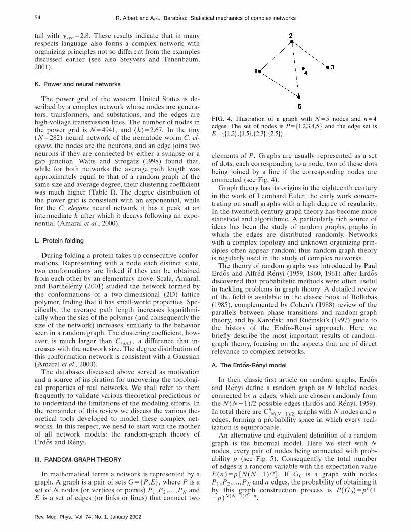
elements of P . Graphs are usually represented as a setof dots, each corresponding to a node, two of these dotsbeing joined by a line if the corresponding nodes areconnected (see Fig. 4).
Graph theory has its origins in the eighteenth centuryin the work of Leonhard Euler, the early work concen-trating on small graphs with a high degree of regularity.In the twentieth century graph theory has become morestatistical and algorithmic. A particularly rich source ofideas has been the study of random graphs, graphs inwhich the edges are distributed randomly. Networkswith a complex topology and unknown organizing prin-ciples often appear random; thus random-graph theoryis regularly used in the study of complex networks.
The theory of random graphs was introduced by PaulErdos and Alfred Renyi (1959, 1960, 1961) after Erdosdiscovered that probabilistic methods were often usefulin tackling problems in graph theory. A detailed reviewof the field is available in the classic book of Bollobas(1985), complemented by Cohen’s (1988) review of theparallels between phase transitions and random-graphtheory, and by Karonski and Rucinski’s (1997) guide tothe history of the Erdos-Renyi approach. Here webriefly describe the most important results of random-graph theory, focusing on the aspects that are of directrelevance to complex networks.
A. The Erdos-Renyi model
In their classic first article on random graphs, Erdosand Renyi define a random graph as N labeled nodesconnected by n edges, which are chosen randomly fromthe N(N21)/2 possible edges (Erdos and Renyi, 1959).In total there are C @N(N21)/2#
n graphs with N nodes and nedges, forming a probability space in which every real-ization is equiprobable.
An alternative and equivalent definition of a randomgraph is the binomial model. Here we start with Nnodes, every pair of nodes being connected with prob-ability p (see Fig. 5). Consequently the total numberof edges is a random variable with the expectation valueE(n)5p @N(N21)/2# . If G0 is a graph with nodesP1 ,P2 ,. . . ,PN and n edges, the probability of obtaining itby this graph construction process is P(G0)5pn(12p)N(N21)/2 2n.
FIG. 4. Illustration of a graph with N55 nodes and n54edges. The set of nodes is P5$1,2,3,4,5% and the edge set isE5$$1,2%,$1,5%,$2,3%,$2,5%%.

55R. Albert and A.-L. Barabasi: Statistical mechanics of complex networks
Random-graph theory studies the properties of theprobability space associated with graphs with N nodes asN→` . Many properties of such random graphs can bedetermined using probabilistic arguments. In this respectErdos and Renyi used the definition that almost everygraph has a property Q if the probability of having Qapproaches 1 as N→` . Among the questions addressedby Erdos and Renyi, some have direct relevance to anunderstanding of complex networks as well, such as: Is atypical graph connected? Does it contain a triangle ofconnected nodes? How does its diameter depend on itssize?
In the mathematical literature the construction of arandom graph is often called an evolution: starting witha set of N isolated vertices, the graph develops by thesuccessive addition of random edges. The graphs ob-tained at different stages of this process correspond tolarger and larger connection probabilities p , eventuallyobtaining a fully connected graph [having the maximumnumber of edges n5N(N21)/2] for p→1. The maingoal of random-graph theory is to determine at whatconnection probability p a particular property of a graphwill most likely arise. The greatest discovery of Erdosand Renyi was that many important properties of ran-dom graphs appear quite suddenly. That is, at a givenprobability either almost every graph has some propertyQ (e.g., every pair of nodes is connected by a path ofconsecutive edges) or, conversely, almost no graph has it.The transition from a property’s being very unlikely toits being very likely is usually swift. For many such prop-erties there is a critical probability pc(N). If p(N)grows more slowly than pc(N) as N→` , then almostevery graph with connection probability p(N) fails tohave Q . If p(N) grows somewhat faster than pc(N),then almost every graph has the property Q . Thus the
FIG. 5. Illustration of the graph evolution process for theErdos-Renyi model. We start with N510 isolated nodes (up-per panel), then connect every pair of nodes with probabilityp . The lower panel of the figure shows two different stages inthe graph’s development, corresponding to p50.1 and p50.15. We can notice the emergence of trees (a tree of order 3,drawn with long-dashed lines) and cycles (a cycle of order 3,drawn with short-dashed lines) in the graph, and a connectedcluster that unites half of the nodes at p50.1551.5/N .
Rev. Mod. Phys., Vol. 74, No. 1, January 2002
probability that a graph with N nodes and connectionprobability p5p(N) has property Q satisfies
limN→`
PN ,p~Q !5H 0 ifp~N !
pc~N !→0
1 ifp~N !
pc~N !→` .
(4)
An important note is in order here. Physicists trainedin critical phenomena will recognize in pc(N) the criticalprobability familiar in percolation. In the physics litera-ture the system is usually viewed at a fixed system size Nand then the different regimes in Eq. (4) reduce to thequestion of whether p is smaller or larger than pc . Theproper value of pc , that is, the limit pc5pc(N→`), isobtained by finite size scaling. The basis of this proce-dure is the assumption that this limit exists, reflectingthe fact that ultimately the percolation threshold is inde-pendent of the system size. This is usually the case infinite-dimensional systems, which include most physicalsystems of interest for percolation theory and criticalphenomena. In contrast, networks are by definition infi-nite dimensional: the number of neighbors a node canhave increases with the system size. Consequently inrandom-graph theory the occupation probability is de-fined as a function of the system size: p represents thefraction of the edges that are present from the possibleN(N21)/2. Larger graphs with the same p will containmore edges, and consequently properties like the ap-pearance of cycles could occur for smaller p in largegraphs than in smaller ones. This means that for manyproperties Q in random graphs there is no unique,N-independent threshold, but we have to define athreshold function that depends on the system size, andpc(N→`)→0. However, we shall see that the averagedegree of the graph
^k&52n/N5p~N21 !.pN (5)
does have a critical value that is independent of the sys-tem size. In the coming subsection we illustrate theseideas by looking at the emergence of various subgraphsin random graphs.
B. Subgraphs
The first property of random graphs to be studied byErdos and Renyi (1959) was the appearance of sub-graphs. A graph G1 consisting of a set P1 of nodes and aset E1 of edges is a subgraph of a graph G5$P ,E% if allnodes in P1 are also nodes of P and all edges in E1 arealso edges of E . The simplest examples of subgraphs arecycles, trees, and complete subgraphs (see Fig. 5). Acycle of order k is a closed loop of k edges such thatevery two consecutive edges and only those have a com-mon node. That is, graphically a triangle is a cycle oforder 3, while a rectangle is a cycle of order 4. The av-erage degree of a cycle is equal to 2, since every nodehas two edges. The opposite of cycles are the trees,which cannot form closed loops. More precisely, a graphis a tree of order k if it has k nodes and k21 edges,

56 R. Albert and A.-L. Barabasi: Statistical mechanics of complex networks
and none of its subgraphs is a cycle. The average degreeof a tree of order k is ^k&5222/k , approaching 2 forlarge trees. Complete subgraphs of order k contain knodes and all the possible k(k21)/2 edges—in otherwords, they are completely connected.
Let us consider the evolution process described in Fig.5 for a graph G5GN ,p . We start from N isolated nodes,then connect every pair of nodes with probability p . Forsmall connection probabilities the edges are isolated, butas p , and with it the number of edges, increases, twoedges can attach at a common node, forming a tree oforder 3. An interesting problem is to determine the criti-cal probability pc(N) at which almost every graph Gcontains a tree of order 3. Most generally we can askwhether there is a critical probability that marks the ap-pearance of arbitrary subgraphs consisting of k nodesand l edges.
In random-graph theory there is a rigorously provenanswer to this question (Bollobas, 1985). Consider a ran-dom graph G5GN ,p . In addition, consider a smallgraph F consisting of k nodes and l edges. In principle,the random graph G can contain several such subgraphsF . Our first goal is to determine how many such sub-graphs exist. The k nodes can be chosen from the totalnumber of nodes N in CN
k ways and the l edges areformed with probability pl. In addition, we can permutethe k nodes and potentially obtain k! new graphs (thecorrect value is k!/a , where a is the number of graphsthat are isomorphic to each other). Thus the expectednumber of subgraphs F contained in G is
E~X !5CNk k!
apl.
Nkpl
a. (6)
This notation suggests that the actual number of suchsubgraphs, X , can be different from E(X), but in themajority of cases it will be close to it. Note that thesubgraphs do not have to be isolated, i.e., there can existedges with one node inside the subgraph but the otheroutside of it.
Equation (6) indicates that if p(N) is such thatp(N)Nk/l→0 as N→0, the expected number of sub-graphs E(X)→0, i.e., almost none of the random graphscontains a subgraph F . However, if p(N)5cN2k/l, themean number of subgraphs is a finite number, denotedby l5cl/a , indicating that this function might be thecritical probability. The validity of this finding can betested by calculating the distribution of subgraph num-bers, Pp(X5r), obtaining (Bollobas, 1985)
limN→`
Pp~X5r !5e2llr
r!. (7)
The probability that G contains at least one subgraph Fis then
Pp~G.F !5(r51
`
Pp~X5r !512e2l, (8)
which converges to 1 as c increases. For p values satis-fying pNk/l→` the probability Pp(G.F) converges to
Rev. Mod. Phys., Vol. 74, No. 1, January 2002
1. Thus, indeed, the critical probability at which almostevery graph contains a subgraph with k nodes and ledges is pc(N)5cN2k/l.
A few important special cases directly follow from Eq.(8):
(a) The critical probability of having a tree of order kis pc(N)5cN2k/(k21);
(b) The critical probability of having a cycle of orderk is pc(N)5cN21;
(c) The critical probability of having a complete sub-graph of order k is pc(N)5cN22/(k21).
C. Graph evolution
It is instructive to look at the results discussed abovefrom a different point of view. Consider a random graphwith N nodes and assume that the connection probabil-ity p(N) scales as Nz, where z is a tunable parameterthat can take any value between 2` and 0 (Fig. 6). Forz less than 23/2 almost all graphs contain only isolatednodes and edges. When z passes through 23/2, trees oforder 3 suddenly appear. When z reaches 24/3, trees oforder 4 appear, and as z approaches 21, the graph con-tains trees of larger and larger order. However, as longas z,21, such that the average degree of the graph^k&5pN→0 as N→` , the graph is a union of disjointtrees, and cycles are absent. Exactly when z passesthrough 21, corresponding to ^k&5const, even though zis changing smoothly, the asymptotic probability ofcycles of all orders jumps from 0 to 1. Cycles of order 3can also be viewed as complete subgraphs of order 3.Complete subgraphs of order 4 appear at z522/3, andas z continues to increase, complete subgraphs of largerand larger order continue to emerge. Finally, as z ap-proaches 0, the graph contains complete subgraphs of allfinite order.
Further results can be derived for z521, i.e., whenwe have p}N21 and the average degree of the nodes is^k&5const. For p}N21 a random graph contains treesand cycles of all order, but so far we have not discussedthe size and structure of a typical graph component. Acomponent of a graph is by definition a connected, iso-
FIG. 6. The threshold probabilities at which different sub-graphs appear in a random graph. For pN3/2→0 the graphconsists of isolated nodes and edges. For p;N23/2 trees oforder 3 appear, while for p;N24/3 trees of order 4 appear. Atp;N21 trees of all orders are present, and at the same timecycles of all orders appear. The probability p;N22/3 marks theappearance of complete subgraphs of order 4 and p;N21/2
corresponds to complete subgraphs of order 5. As z ap-proaches 0, the graph contains complete subgraphs of increas-ing order.
57R. Albert and A.-L. Barabasi: Statistical mechanics of complex networks
lated subgraph, also called a cluster in network researchand percolation theory. As Erdos and Renyi (1960)show, there is an abrupt change in the cluster structureof a random graph as ^k& approaches 1.
If 0,^k&,1, almost surely all clusters are either treesor clusters containing exactly one cycle. Although cyclesare present, almost all nodes belong to trees. The meannumber of clusters is of order N2n , where n is thenumber of edges, i.e., in this range when a new edge isadded the number of clusters decreases by 1. The largestcluster is a tree, and its size is proportional to ln N.
When ^k& passes the threshold ^k&c51, the structureof the graph changes abruptly. While for ^k&,1 thegreatest cluster is a tree, for ^k&c51 it has approxi-mately N2/3 nodes and has a rather complex structure.Moreover for ^k&.1 the greatest (giant) cluster has @12f(^k&)#N nodes, where f(x) is a function that de-creases exponentially from f(1)51 to 0 for x→` . Thusa finite fraction S512f(^k&) of the nodes belongs tothe largest cluster. Except for this giant cluster, all otherclusters are relatively small, most of them being trees,the total number of nodes belonging to trees beingNf(^k&). As ^k& increases, the small clusters coalesceand join the giant cluster, the smaller clusters having thehigher chance of survival.
Thus at pc.1/N the random graph changes its topol-ogy abruptly from a loose collection of small clusters toa system dominated by a single giant cluster. The begin-ning of the supercritical phase was studied by Bollobas(1984), Kolchin (1986), and Luczak (1990). Their resultsshow that in this region the largest cluster clearly sepa-rates from the rest of the clusters, its size S increasingproportionally with the separation from the criticalprobability,
S}~p2pc!. (9)
As we shall see in Sec. IV.F, this dependence is analo-gous to the scaling of the percolation probability ininfinite-dimensional percolation.
D. Degree distribution
Erdos and Renyi (1959) were the first to study thedistribution of the maximum and minimum degree in arandom graph, the full degree distribution being derivedlater by Bollobas (1981).
In a random graph with connection probability p thedegree ki of a node i follows a binomial distributionwith parameters N21 and p :
P~ki5k !5CN21k pk~12p !N212k. (10)
This probability represents the number of ways in whichk edges can be drawn from a certain node: the probabil-ity of k edges is pk, the probability of the absence ofadditional edges is (12p)N212k, and there are CN21
k
equivalent ways of selecting the k end points for theseedges. Furthermore, if i and j are different nodes, P(ki5k) and P(kj5k) are close to being independent ran-dom variables. To find the degree distribution of thegraph, we need to study the number of nodes with de-
Rev. Mod. Phys., Vol. 74, No. 1, January 2002
gree k ,Xk . Our main goal is to determine the probabil-ity that Xk takes on a given value, P(Xk5r).
According to Eq. (10), the expectation value of thenumber of nodes with degree k is
E~Xk!5NP~ki5k !5lk , (11)
where
lk5NCN21k pk~12p !N212k. (12)
As in the derivation of the existence conditions ofsubgraphs (see Sec. III.B), the distribution of the Xkvalues, P(Xk5r), approaches a Poisson distribution,
P~Xk5r !5e2lklk
r
r!. (13)
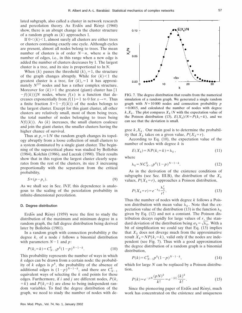
Thus the number of nodes with degree k follows a Pois-son distribution with mean value lk . Note that the ex-pectation value of the distribution (13) is the function lkgiven by Eq. (12) and not a constant. The Poisson dis-tribution decays rapidly for large values of r , the stan-dard deviation of the distribution being sk5Alk. With abit of simplification we could say that Eq. (13) impliesthat Xk does not diverge much from the approximativeresult Xk5NP(ki5k), valid only if the nodes are inde-pendent (see Fig. 7). Thus with a good approximationthe degree distribution of a random graph is a binomialdistribution,
P~k !5CN21k pk~12p !N212k, (14)
which for large N can be replaced by a Poisson distribu-tion,
P~k !.e2pN~pN !k
k!5e2^k&
^k&k
k!. (15)
Since the pioneering paper of Erdos and Renyi, muchwork has concentrated on the existence and uniqueness
FIG. 7. The degree distribution that results from the numericalsimulation of a random graph. We generated a single randomgraph with N510 000 nodes and connection probability p50.0015, and calculated the number of nodes with degreek ,Xk . The plot compares Xk /N with the expectation value ofthe Poisson distribution (13), E(Xk)/N5P(ki5k), and wecan see that the deviation is small.

58 R. Albert and A.-L. Barabasi: Statistical mechanics of complex networks
of the minimum and maximum degree of a randomgraph. The results indicate that for a large range of pvalues both the maximum and the minimum degrees aredetermined and finite. For example, if p(N);N2121/k
(and thus the graph is a set of isolated trees of order atmost k11), almost no graph has nodes with degreehigher than k . At the other extreme, if p5$ln(N)1k ln@ln(N)#1c%/N, almost every random graph has aminimum degree of at least k . Furthermore, for a suffi-ciently high p , respectively, if pN/ln(N)→`, the maxi-mum degree of almost all random graphs has the sameorder of magnitude as the average degree. Thus, despitethe fact that the position of the edges is random, a typi-cal random graph is rather homogeneous, the majorityof the nodes having the same number of edges.
E. Connectedness and diameter
The diameter of a graph is the maximal distance be-tween any pair of its nodes. Strictly speaking, the diam-eter of a disconnected graph (i.e., one made up of sev-eral isolated clusters) is infinite, but it can be defined asthe maximum diameter of its clusters. Random graphstend to have small diameters, provided p is not toosmall. The reason for this is that a random graph is likelyto be spreading: with large probability the number ofnodes at a distance l from a given node is not muchsmaller than ^k& l. Equating ^k& l with N we find that thediameter is proportional to ln(N)/ln(^k&); thus it dependsonly logarithmically on the number of nodes.
The diameter of a random graph has been studied bymany authors (see Chung and Lu, 2001). A general con-clusion is that for most values of p , almost all graphswith the same N and p have precisely the same diameter.This means that when we consider all graphs with Nnodes and connection probability p , the range of valuesin which the diameters of these graphs can vary is verysmall, usually concentrated around
d5ln~N !
ln~pN !5
ln~N !
ln~^k&!. (16)
Below we summarize a few important results:
• If ^k&5pN,1, a typical graph is composed of isolatedtrees and its diameter equals the diameter of a tree.
• If ^k&.1, a giant cluster appears. The diameter of thegraph equals the diameter of the giant cluster if ^k&>3.5, and is proportional to ln(N)/ln(^k&).
• If ^k&>ln(N), almost every graph is totally connected.The diameters of the graphs having the same N and^k& are concentrated on a few values aroundln(N)/ln(^k&).
Another way to characterize the spread of a randomgraph is to calculate the average distance between anypair of nodes, or the average path length. One expectsthat the average path length scales with the number ofnodes in the same way as the diameter,
l rand;ln~N !
ln~^k&!. (17)
Rev. Mod. Phys., Vol. 74, No. 1, January 2002
In Sec. II we presented evidence that the average pathlength of real networks is close to the average pathlength of random graphs with the same size. Equation(17) gives us an opportunity to better compare randomgraphs and real networks (see Newman 2001a, 2001c).According to Eq. (17), the product l rand ln(^k&) is equalto ln(N), so plotting l rand ln(^k&) as a function of ln(N)for random graphs of different sizes gives a straight lineof slope 1. In Fig. 8 we plot a similar product for severalreal networks, l real log(^k&), as a function of the net-work size, comparing it with the prediction of Eq. (17).We can see that the trend of the data is similar to thetheoretical prediction, and with several exceptions Eq.(17) gives a reasonable first estimate.
F. Clustering coefficient
As we mentioned in Sec. II, complex networks exhibita large degree of clustering. If we consider a node in arandom graph and its nearest neighbors, the probabilitythat two of these neighbors are connected is equal to theprobability that two randomly selected nodes are con-nected. Consequently the clustering coefficient of a ran-dom graph is
Crand5p5^k&N
. (18)
According to Eq. (18), if we plot the ratio Crand /^k&as a function of N for random graphs of different sizes,on a log-log plot they will align along a straight line ofslope 21. In Fig. 9 we plot the ratio of the clusteringcoefficient of real networks and their average degree asa function of their size, comparing it with the predictionof Eq. (18). The plot convincingly indicates that real net-works do not follow the prediction of random graphs.The fraction C/^k& does not decrease as N21; instead, itappears to be independent of N . This property is char-
FIG. 8. Comparison between the average path lengths of realnetworks and the prediction (17) of random-graph theory(dashed line). For each symbol we indicate the correspondingnumber in Table I or Table II: small s, I.12; large s, I.13; !,I.17; small h, I.10; medium h, I.11; large h, II.13; small d, II.6;medium d, I.2; 3 , I.16; small n, I.7; small j, I.15; large n, I.4;small v, I.5; large v, I.6; large d, II.6; small l, I.1; small x,I.7; ,, I.3; medium l, II.1; large j, I.14; large x, I.5; large l,II.3.

59R. Albert and A.-L. Barabasi: Statistical mechanics of complex networks
acteristic of large ordered lattices, whose clustering co-efficient depends only on the coordination number ofthe lattice and not their size (Watts and Strogatz, 1998).
G. Graph spectra
Any graph G with N nodes can be represented by itsadjacency matrix A(G) with N3N elements Aij , whosevalue is Aij5Aji51 if nodes i and j are connected, and0 otherwise. The spectrum of graph G is the set of ei-genvalues of its adjacency matrix A(G). A graph withN nodes has N eigenvalues l j , and it is useful to defineits spectral density as
r~l!51N (
j51
N
d~l2l j!, (19)
which approaches a continuous function if N→` . Theinterest in spectral properties is related to the fact thatthe spectral density can be directly linked to the graph’stopological features, since its kth moment can be writtenas
1N (
j51
N
~l j!k5
1N (
i1 ,i2 ,.. . ,ik
Ai1 ,i2Ai2i3
¯Aiki1, (20)
i.e., the number of paths returning to the same node inthe graph. Note that these paths can contain nodes thatwere already visited.
Let us consider a random graph GN ,p satisfyingp(N)5cN2z. For z,1 there is an infinite cluster in thegraph (see Sec. III.C), and as N→` , any node belongsalmost surely to the infinite cluster. In this case the spec-tral density of the random graph converges to a semicir-cular distribution (Fig. 10),
r~l!5H A4Np~12p !2l2
2pNp~12p !if ulu,2ANp~12p !
0 otherwise.(21)
Known as Wigner’s law (see Wigner, 1955, 1957, 1958) orthe semicircle law, Eq. (21) has many applications in
FIG. 9. Comparison between the clustering coefficients of realnetworks and random graphs. All networks from Table I areincluded in the figure, the symbols being the same as in Fig. 8.The dashed line corresponds to Eq. (18).
Rev. Mod. Phys., Vol. 74, No. 1, January 2002
quantum, statistical, and solid-state physics (Mehta,1991; Crisanti et al., 1993; Guhr et al., 1998). The largest(principal) eigenvalue, l1 , is isolated from the bulk ofthe spectrum, and it increases with the network size aspN .
When z.1 the spectral density deviates from thesemicircle law. The most striking feature of r(l) is thatits odd moments are equal to zero, indicating that theonly way that a path comes back to the original node isif it returns following exactly the same nodes. This is asalient feature of a tree structure, and, indeed, in Sec.III.B we have seen that in this case the random graph iscomposed of trees.
IV. PERCOLATION THEORY
One of the most interesting findings of random-graphtheory is the existence of a critical probability at which agiant cluster forms. Translated into network language,the theory indicates the existence of a critical probabilitypc such that below pc the network is composed of iso-lated clusters but above pc a giant cluster spans the en-tire network. This phenomenon is markedly similar to apercolation transition, a topic much studied both inmathematics and in statistical mechanics (Stauffer andAharony, 1992; Bunde and Havlin, 1994, 1996; Grim-mett, 1999; ben Avraham and Havlin, 2000). Indeed, apercolation transition and the emergence of a giant clus-ter are the same phenomenon expressed in different lan-guages. Percolation theory, however, does not simply re-produce the predictions of random-graph theory. Askingquestions from a different perspective, it addresses sev-eral issues that are crucial for understanding real net-works but are not discussed by random graph theory.Consequently it is important to review the predictions of
FIG. 10. Rescaled spectral density of three random graphshaving p50.05 and size N5100 (solid line), N5300 (long-dashed line), and N51000 (short-dashed line). The isolatedpeak corresponds to the principal eigenvalue. After Farkaset al. (2001).
60 R. Albert and A.-L. Barabasi: Statistical mechanics of complex networks
percolation theory relevant to networks, as they are cru-cial for an understanding of important aspects of thenetwork topology.
A. Quantities of interest in percolation theory
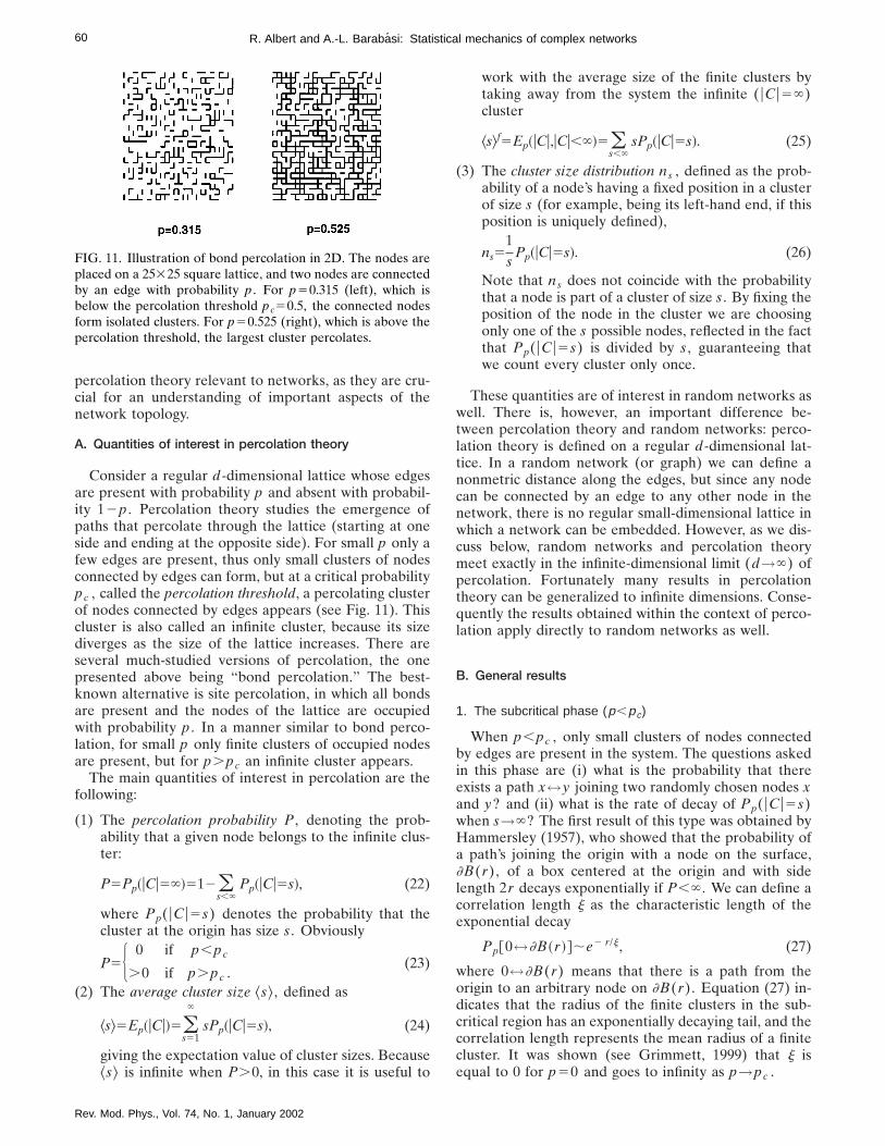
Consider a regular d-dimensional lattice whose edgesare present with probability p and absent with probabil-ity 12p . Percolation theory studies the emergence ofpaths that percolate through the lattice (starting at oneside and ending at the opposite side). For small p only afew edges are present, thus only small clusters of nodesconnected by edges can form, but at a critical probabilitypc , called the percolation threshold, a percolating clusterof nodes connected by edges appears (see Fig. 11). Thiscluster is also called an infinite cluster, because its sizediverges as the size of the lattice increases. There areseveral much-studied versions of percolation, the onepresented above being ‘‘bond percolation.’’ The best-known alternative is site percolation, in which all bondsare present and the nodes of the lattice are occupiedwith probability p . In a manner similar to bond perco-lation, for small p only finite clusters of occupied nodesare present, but for p.pc an infinite cluster appears.
The main quantities of interest in percolation are thefollowing:
(1) The percolation probability P , denoting the prob-ability that a given node belongs to the infinite clus-ter:
P5Pp~uCu5`!512(s,`
Pp~uCu5s!, (22)
where Pp(uCu5s) denotes the probability that thecluster at the origin has size s . Obviously
P5H 0 if p,pc
.0 if p.pc .(23)
(2) The average cluster size ^s&, defined as
^s&5Ep~uCu!5(s51
`
sPp~uCu5s!, (24)
giving the expectation value of cluster sizes. Because^s& is infinite when P.0, in this case it is useful to
FIG. 11. Illustration of bond percolation in 2D. The nodes areplaced on a 25325 square lattice, and two nodes are connectedby an edge with probability p . For p50.315 (left), which isbelow the percolation threshold pc50.5, the connected nodesform isolated clusters. For p50.525 (right), which is above thepercolation threshold, the largest cluster percolates.
Rev. Mod. Phys., Vol. 74, No. 1, January 2002
work with the average size of the finite clusters bytaking away from the system the infinite (uCu5`)cluster
^s&f5Ep~uCu,uCu,`!5(s,`
sPp~uCu5s!. (25)
(3) The cluster size distribution ns , defined as the prob-ability of a node’s having a fixed position in a clusterof size s (for example, being its left-hand end, if thisposition is uniquely defined),
ns51s
Pp~uCu5s!. (26)
Note that ns does not coincide with the probabilitythat a node is part of a cluster of size s . By fixing theposition of the node in the cluster we are choosingonly one of the s possible nodes, reflected in the factthat Pp(uCu5s) is divided by s , guaranteeing thatwe count every cluster only once.
These quantities are of interest in random networks aswell. There is, however, an important difference be-tween percolation theory and random networks: perco-lation theory is defined on a regular d-dimensional lat-tice. In a random network (or graph) we can define anonmetric distance along the edges, but since any nodecan be connected by an edge to any other node in thenetwork, there is no regular small-dimensional lattice inwhich a network can be embedded. However, as we dis-cuss below, random networks and percolation theorymeet exactly in the infinite-dimensional limit (d→`) ofpercolation. Fortunately many results in percolationtheory can be generalized to infinite dimensions. Conse-quently the results obtained within the context of perco-lation apply directly to random networks as well.
B. General results
1. The subcritical phase (p,pc)
When p,pc , only small clusters of nodes connectedby edges are present in the system. The questions askedin this phase are (i) what is the probability that thereexists a path x↔y joining two randomly chosen nodes xand y? and (ii) what is the rate of decay of Pp(uCu5s)when s→`? The first result of this type was obtained byHammersley (1957), who showed that the probability ofa path’s joining the origin with a node on the surface,]B(r), of a box centered at the origin and with sidelength 2r decays exponentially if P,` . We can define acorrelation length j as the characteristic length of theexponential decay
Pp@0↔]B~r !#;e2 r/j, (27)
where 0↔]B(r) means that there is a path from theorigin to an arbitrary node on ]B(r). Equation (27) in-dicates that the radius of the finite clusters in the sub-critical region has an exponentially decaying tail, and thecorrelation length represents the mean radius of a finitecluster. It was shown (see Grimmett, 1999) that j isequal to 0 for p50 and goes to infinity as p→pc .
61R. Albert and A.-L. Barabasi: Statistical mechanics of complex networks
The exponential decay of cluster radii implies that theprobability that a cluster has size s , Pp(uCu5s), alsodecays exponentially for large s :
Pp~ uCu5s !;e2a(p)s as s→` , (28)
where a(p)→` as p→0 and a(pc)50.
2. The supercritical phase (p.pc)
For P.0 there is exactly one infinite cluster (Burtonand Keane, 1989). In this supercritical phase the previ-ously studied quantities are dominated by the contribu-tion of the infinite cluster; thus it is useful to study thecorresponding probabilities in terms of finite clusters.The probability that there is a path from the origin tothe surface of a box of edge length 2r that is not part ofthe infinite cluster decays exponentially as
Pp@0↔]B~r !,uCu,`#;e2 r/j. (29)
Unlike the subcritical phase, though, the decay of thecluster sizes, Pp(uCu5s,`), follows a stretch exponen-tial, e2b(p)s(d21)/d
, offering the first important quantitythat depends on the dimensionality of the lattice, buteven this dependence vanishes as d→` , and the clustersize distribution decays exponentially as in the subcriti-cal phase.
C. Exact solutions: Percolation on a Cayley tree
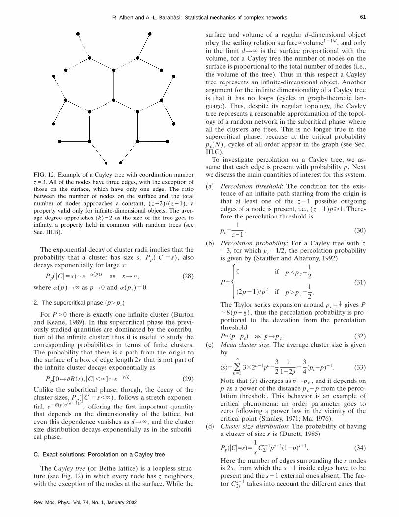
The Cayley tree (or Bethe lattice) is a loopless struc-ture (see Fig. 12) in which every node has z neighbors,with the exception of the nodes at the surface. While the
FIG. 12. Example of a Cayley tree with coordination numberz53. All of the nodes have three edges, with the exception ofthose on the surface, which have only one edge. The ratiobetween the number of nodes on the surface and the totalnumber of nodes approaches a constant, (z22)/(z21), aproperty valid only for infinite-dimensional objects. The aver-age degree approaches ^k&52 as the size of the tree goes toinfinity, a property held in common with random trees (seeSec. III.B).
Rev. Mod. Phys., Vol. 74, No. 1, January 2002
surface and volume of a regular d-dimensional objectobey the scaling relation surface}volume121/d, and onlyin the limit d→` is the surface proportional with thevolume, for a Cayley tree the number of nodes on thesurface is proportional to the total number of nodes (i.e.,the volume of the tree). Thus in this respect a Cayleytree represents an infinite-dimensional object. Anotherargument for the infinite dimensionality of a Cayley treeis that it has no loops (cycles in graph-theoretic lan-guage). Thus, despite its regular topology, the Cayleytree represents a reasonable approximation of the topol-ogy of a random network in the subcritical phase, whereall the clusters are trees. This is no longer true in thesupercritical phase, because at the critical probabilitypc(N), cycles of all order appear in the graph (see Sec.III.C).
To investigate percolation on a Cayley tree, we as-sume that each edge is present with probability p . Nextwe discuss the main quantities of interest for this system.
(a) Percolation threshold: The condition for the exis-tence of an infinite path starting from the origin isthat at least one of the z21 possible outgoingedges of a node is present, i.e., (z21)p>1. There-fore the percolation threshold is
pc51
z21. (30)
(b) Percolation probability: For a Cayley tree with z53, for which pc51/2, the percolation probabilityis given by (Stauffer and Aharony, 1992)
P5H0 if p,pc512
~2p21 !/p2 if p.pc512
.
(31)
The Taylor series expansion around pc5 12 gives P
.8(p2 12 ), thus the percolation probability is pro-
portional to the deviation from the percolationthresholdP}~p2pc! as p→pc . (32)
(c) Mean cluster size: The average cluster size is givenby
^s&5(n51
`
332n21pn532
1122p
534
~pc2p!21. (33)
Note that ^s& diverges as p→pc , and it depends onp as a power of the distance pc2p from the perco-lation threshold. This behavior is an example ofcritical phenomena: an order parameter goes tozero following a power law in the vicinity of thecritical point (Stanley, 1971; Ma, 1976).
(d) Cluster size distribution: The probability of havinga cluster of size s is (Durett, 1985)
Pp~uCu5s!51s
C2ss21ps21~12p!s11. (34)
Here the number of edges surrounding the s nodesis 2s , from which the s21 inside edges have to bepresent and the s11 external ones absent. The fac-tor C2s
s21 takes into account the different cases that
62 R. Albert and A.-L. Barabasi: Statistical mechanics of complex networks
can be obtained when permuting the edges, andthe 1/s is a normalization factor. Since ns5(1/s) Pp(uCu5s), after using Stirling’s formulawe obtain
ns}s25/2ps21~12p !s11. (35)
In the vicinity of the percolation threshold this ex-pression can be approximated as
ns;s25/2e2cs with c}~p2pc!2. (36)
Thus the cluster size distribution follows a powerlaw with an exponential cutoff: only clusters withsize s,sj51/c}(p2pc)22 contribute significantlyto cluster averages. For these clusters, ns is effec-tively equal to ns(pc)}s25/2. Clusters with s@sj
are exponentially rare, and their properties are nolonger dominated by the behavior at pc . The no-tation sj illustrates that as the correlation length jis the characteristic length scale for the cluster di-ameters, sj is an intrinsic characteristic of clustersizes. The correlation length of a tree is not welldefined, but we shall see in the more general casesthat sj and j are related by a simple power law.
D. Scaling in the critical region
The principal ansatz of percolation theory is that eventhe most general percolation problem in any dimensionobeys a scaling relation similar to Eq. (36) near the per-colation threshold. Thus in general the cluster size dis-tribution can be written as
ns~p !;H s2tf2~ up2pcu1/ss ! as p<pc
s2tf1~ up2pcu1/ss ! as p>pc .(37)
Here t and s are critical exponents whose numericalvalue needs to be determined, f2 and f1 are smoothfunctions on [0,`), and f2(0)5f1(0). The results ofSec. IV.B suggest that f2(x).e2Ax and f1(x).e2Bx(d21)/d
for x@1. This ansatz indicates that the roleof sj}up2pcu21/s as a cutoff is the same as in a Cayleytree. The general form (37) contains as a special case theCayley tree (36) with t55/2, s51/2, and f6(x)5e2x.
Another element of the scaling hypothesis is that thecorrelation length diverges near the percolation thresh-old following a power law:
j~p !;up2pcu2n as p→pc . (38)
This ansatz introduces the correlation exponent n andindicates that j and sj are related by a power law sj
5j1/sn. From these two hypotheses we find that the per-colation probability (22) is given by
P;~p2pc!b with b5t22
s, (39)
which scales as a positive power of p2pc for p>pc ;thus it is 0 for p5pc and increases when p.pc . Theaverage size of finite clusters, ^s& f, which can be calcu-lated on both sides of the percolation threshold, obeys
Rev. Mod. Phys., Vol. 74, No. 1, January 2002
^s& f;up2pcu2g with g532t
s, (40)
diverging for p→pc . The exponents b and g are calledthe critical exponents of the percolation probability andaverage cluster size, respectively.
E. Cluster structure
Until now we have discussed cluster sizes and radii,ignoring their internal structure. Let us now consider theperimeter of a cluster t denoting the number of nodessituated on the most external edges (the leaf nodes).The perimeter ts of a very large but finite cluster of sizes scales as (Leath, 1976)
ts5s12p
p1Asz as s→` , (41)
where z51 for p,pc and z5121/d for p.pc . Thusbelow pc the perimeter of a cluster is proportional to itsvolume, a highly irregular property, which is neverthe-less true for trees, including the Cayley tree.
Another way of understanding the unusual structureof finite clusters is by looking at the relation betweentheir radii and volume. The correlation length j is ameasure of the mean cluster radius, and we know that jscales with the cutoff cluster size sj as j}sj
1/ns . Thusfinite clusters are fractals (see Mandelbrot, 1982) be-cause their size does not scale as their radius to the dthpower, but as
s~r !;rdf, (42)
where df51/sn . It can also be shown that at the perco-lation threshold an infinite cluster is still a fractal, but forp.pc it becomes a normal d-dimensional object.
While the cluster radii and the correlation length j aredefined using Euclidian distances on the lattice, thechemical distance is defined as the length of the shortestpath between two arbitrary sites on a cluster (Havlinand Nossal, 1984). Thus the chemical distance is theequivalent of the distance on random graphs. The num-ber of nodes within chemical distance l scales as
s~ l !;l d l , (43)
where d l is called the graph dimension of the cluster.While the fractal dimension df of the Euclidian distanceshas been related to the other critical exponents, no suchrelation has yet been found for the graph dimension d l .
F. Infinite-dimensional percolation
Percolation is known to have a critical dimension dc ,below which some exponents depend on d , but for anydimension above dc the exponents are the same. Whileit is generally believed that the critical dimension of per-colation is dc56, the dimension independence of thecritical exponents is proven rigorously only for d>19(see Hara and Slade, 1990). Thus for d.dc the results ofinfinite-dimensional percolation theory apply, which pre-dict that

63R. Albert and A.-L. Barabasi: Statistical mechanics of complex networks
• P;(p2pc) as p→pc ;• ^s&;(pc2p)21 as p→pc ;• ns;s25/2e2up2pcu2s as p→pc ;• j;up2pcu21/2 as p→pc .
Consequently the critical exponents of infinite-dimensional percolation are t`55/2, s`51/2, and n`51/2. The fractal dimension of an infinite cluster at thepercolation threshold is df54, while the graph dimen-sion is d l 52 (Bunde and Havlin, 1996). Thus the char-acteristic chemical distance on a finite cluster or infinitecluster at the percolation threshold scales with its size as
l ;s2/df5s1/2. (44)
G. Parallels between random-graph theory and percolation
In random-graph theory we study a graph of N nodes,each pair of nodes being connected with probability p .This corresponds to percolation in at most N dimen-sions, such that each two connected nodes are neigh-bors, and the edges between graph nodes are the edgesin the percolation problem. Since random-graph theoryinvestigates the N→` regime, it is analogous to infinite-dimensional percolation.
We have seen in Sec. IV.C that infinite-dimensionalpercolation is similar to percolation on a Cayley tree.The percolation threshold of a Cayley tree is pc51/(z21), where z is the coordination number of the tree. Ina random graph of N nodes the coordination number isN21; thus the ‘‘percolation threshold,’’ denoting theconnection probability at which a giant cluster appears,should be pc.1/N . Indeed, this is exactly the probabilityat which the phase transition leading to a giant compo-nent appears in random graphs, as Erdos and Renyishowed (see Sec. III.C).
Compare the predictions of random-graph theory andinfinite-dimensional percolation, some of which reflect acomplete analogy:
(1) For p,pc51/N
• The probability of a giant cluster in a graph, and of aninfinite cluster in percolation, is equal to 0.
• The clusters of a random graph are trees, while theclusters in percolation have a fractal structure and aperimeter proportional with their volume.
• The largest cluster in a random graph is a tree withln(N) nodes, while in general for percolation Pp(uCu5s);e2s/sj [see Eq. (28) in Sec. IV.B], suggesting thatthe size of the largest cluster scales as ln(N).
(2) For p5pc51/N
• A unique giant cluster or an infinite cluster appears.• The size of the giant cluster is N2/3; while for infinite-
dimensional percolation Pp(uCu5s);s23/2, thus thesize of the largest cluster scales as N2/3.
(3) For p.pc51/N
• The size of the giant cluster is „f(pcN)2f(pN)…N ,where f is an exponentially decreasing function withf(1)51. The size of the infinite cluster is PN}(p2pc)N .
Rev. Mod. Phys., Vol. 74, No. 1, January 2002
• The giant cluster has a complex structure containingcycles, while the infinite cluster is no longer fractal,but compact.
All these correspondences indicate that the phasetransition in random graphs belongs in the same univer-sality class as mean-field percolation. Numerical simula-tions of random graphs (see, for example, Christensenet al., 1998) have confirmed that the critical exponents ofthe phase transition are equal to the critical exponentsof infinite-dimensional percolation. The equivalence ofthese two theories is very important because it offers usdifferent perspectives on the same problem. For ex-ample, it is often of interest to look at the cluster sizedistribution of a random network with a fixed number ofnodes. This question is answered in a simpler way inpercolation theory. However, random-graph theory an-swers questions of major importance for networks, suchas the appearance of trees and cycles, which are largelyignored by percolation theory.
In some cases there is an apparent discrepancy be-tween the predictions of random-graph theory and per-colation theory. For example, percolation theory pre-dicts that the chemical distance between two nodes in aninfinite cluster scales as a power of the size of the cluster[see Eq. (44)]. However, random-graph theory predicts[Eq. (16)] that the diameter of an infinite cluster scaleslogarithmically with its size (see Chung and Lu, 2001).The origin of the apparent discrepancy is that these twopredictions refer to different regimes. While Eq. (44) isvalid only when the infinite cluster is barely formed [i.e.,p5pc and ^k&51] and is still a fractal, the prediction ofrandom-graph theory is valid only well beyond the per-colation transition, when ^k&@1. Consequently, by usingthese two limits we can address the evolution of thechemical distance in an infinite cluster (see Cohen et al.,2001). Thus for a full characterization of random net-works we need to be aware of both of these complemen-tary approaches.
V. GENERALIZED RANDOM GRAPHS
In Sec. II we have seen that real networks differ fromrandom graphs in that often their degree distributionfollows a power law P(k);k2g. Since power laws arefree of a characteristic scale, these networks are called‘‘scale-free networks’’ (Barabasi and Albert, 1999; Bara-basi, Albert, and Jeong, 1999). As random graphs do notcapture the scale-free character of real networks, weneed a different model to describe these systems. Oneapproach is to generalize random graphs by constructinga model that has the degree distribution as an input butis random in all other respects. In other words, the edgesconnect randomly selected nodes, with the constraintthat the degree distribution is restricted to a power law.The theory of such semirandom graphs should answersimilar questions to those asked by Erdos and Renyi andpercolation theory (see Secs. III, IV): Is there a thresh-old at which a giant cluster appears? How do the sizeand topology of the clusters evolve? When does the

64 R. Albert and A.-L. Barabasi: Statistical mechanics of complex networks
graph become connected? In addition, we need to deter-mine the average path length and clustering coefficientof such graphs.
The first step in developing such a theory is to identifythe relevant parameter that, together with the networksize, gives a statistically complete characterization of thenetwork. In the case of random graphs this parameter isthe connection probability (see Sec. III.A); for percola-tion theory it is the bond occupation probability (seeSec. IV). Since the only restriction for these graphs isthat their degree distribution follow a power law, theexponent g of the degree distribution could play the roleof the control parameter. Accordingly, we study scale-free random networks by systematically varying g andsee if there is a threshold value of g at which the net-works’ important properties abruptly change.
We start by sketching a few intuitive expectations.Consider a large network with degree distributionP(k);k2g, in which g decreases from ` to 0. The av-erage degree of the network, or equivalently, the num-ber of edges, increases as g decreases, since ^k&;kmax
2g12 , where kmax,N is the maximum degree of thegraph. This is very similar to the graph evolution processdescribed by Erdos and Renyi (see Sec. III.C). Conse-quently we expect that, while at large g the networkconsists of isolated small clusters, there is a critical valueof g at which a giant cluster forms, and at an evensmaller g the network becomes completely connected.
The theory of random graphs with given degree se-quence is relatively recent. One of the first results is dueto Luczak (1992), who showed that almost all randomgraphs with a fixed degree distribution and no nodes ofdegree smaller than 2 have a unique giant cluster. Mol-loy and Reed (1995, 1998) have proven that for a ran-dom graph with degree distribution P(k) an infinitecluster emerges almost surely when
Q[ (k>1
k~k22 !P~k !.0, (45)
provided that the maximum degree is less than N1/4. Themethod of Molloy and Reed was applied to randomgraphs with power-law degree distributions by Aiello,Chung, and Lu (2000). As we show next, their results arein excellent agreement with the expectations outlinedabove.
A. Thresholds in a scale-free random graph
Aiello, Chung, and Lu (2000) introduce a two-parameter random-graph model P(a ,g) defined as fol-lows: Let Nk be the number of nodes with degree k .P(a ,g) assigns uniform probability to all graphs withNk5eak2g. Thus in this model it is not the total numberof nodes that is specified—along with the exponentg—from the beginning, but the number of nodes withdegree 1. Nevertheless the number of nodes and edgesin the graph can be deduced, noting that the maximumdegree of the graph is ea/g. To find the condition for theappearance of a giant cluster in this model, we insert
Rev. Mod. Phys., Vol. 74, No. 1, January 2002
P(a ,g) into Eq. (45), finding as a solution g053.478 75 . . . . Thus when g.g0 the random graph al-most surely has no infinite cluster. On the other hand,when g,g0 there is almost surely a unique infinite clus-ter.
An important question is whether the graph is con-nected or not. Certainly for g.g0 the graph is discon-nected as it is made of independent finite clusters. In the0,g,g0 regime Aiello, Chung, and Lu (2000) study thesize of the second-largest cluster, finding that for 2<g<g0 the second-largest cluster almost surely has a sizeof the order of ln N; thus it is relatively small. However,for 1,g,2 almost surely every node with degreegreater than ln(N) belongs to the infinite cluster. Thesecond-largest cluster has a size of order 1, i.e., its sizedoes not increase as the size of the graph goes to infinity.This means that the fraction of nodes in the infinite clus-ter approaches 1 as the system size increases; thus thegraph becomes totally connected in the limit of infinitesystem size. Finally, for 0,g,1 the graph is almostsurely connected.
B. Generating function formalism
A general approach to random graphs with given de-gree distribution was developed by Newman, Strogatz,and Watts (2001) using a generating function formalism(Wilf, 1990). The generating function of the degree dis-tribution,
G0~x !5 (k50
`
P~k !xk, (46)
encapsulates all the information contained in P(k),since
P~k !51k!
dkG0
dxk Ux50
. (47)
An important quantity for studying cluster structure isthe generating function for the degree distribution of thenearest neighbors of a randomly selected node. This canbe obtained in the following way: a randomly selectededge reaches a node with degree k with probability pro-portional to kP(k) (i.e., it is easier to find a well-connected node). If we start from a randomly chosennode and follow each of the edges starting from it, thenthe nodes we visit have their degree distribution gener-ated by kP(k). In addition, the generating function willcontain a term xk21 [instead of xk as in Eq. (46)] be-cause we have to discount the edge through which wereached the node. Thus the distribution of outgoingedges is generated by the function
G1~x !5
(k
kP~k !xk21
(k
kP~k !
51
^k&G08~x !. (48)
The average number of first neighbors is equal to theaverage degree of the graph,
z15^k&5(k
kP~k !5G08~1 !. (49)

65R. Albert and A.-L. Barabasi: Statistical mechanics of complex networks
1. Component sizes and phase transitions
When we identify a cluster using a burning (breadth-first-search) algorithm, we start from an arbitrary nodeand follow its edges until we reach its nearest neighbors.We record these nodes as part of the cluster, then followtheir outside edges (avoiding the already recordednodes) and record the nodes we arrive at as next-nearestneighbors of the starting node. This process is repeateduntil no new nodes are found, the set of identified nodesforming an isolated cluster. This algorithm is implicitlyincorporated into the generating function method. Thegenerating function, H1(x), for the size distribution ofthe clusters reached by following a random edge satisfiesthe iterative equation
H1~x !5
(k
kP~k !@H1~x !#k
(k
kP~k !
5xG1@H1~x !# . (50)
Here kP(k) is proportional to the probability that arandom edge arrives at a node with degree k , and@H1(x)#k represents the k ways in which the cluster canbe continued recursively (i.e., by finding the nearestneighbors of a previously found node). If we start at arandomly chosen node then we have one such cluster atthe end of each edge leaving that node, and hence thegenerating function for the size of the whole cluster is
H0~x !5x(k
P~k !@H1~x !#k5xG0@H1~x !# . (51)
When there is no giant cluster present in the graph,the average cluster size is given by
^s&5H08~1 !511G08~1 !
12G18~1 !. (52)
This expression diverges when G18(1)51, indicating theappearance of a giant cluster. Substituting the definitionof G0(x) we can write the condition of the emergence ofthe giant cluster as
(k
k~k22 !P~k !50, (53)
identical to Eq. (45) derived by Molloy and Reed (1995).Equation (53) gives an implicit relation for the criticaldegree distribution of a random graph: For any degreedistribution for which the sum on the left-hand side isnegative, no giant cluster is present in the graph, butdegree distributions that give a positive sum lead to theappearance of a giant cluster.
When a giant cluster is present, H0(x) generates theprobability distribution of the finite clusters. This meansthat H0(1) is no longer unity but instead takes on thevalue 12S , where S is the fraction of nodes in the giantcluster. We can use this to calculate the size of the giantcluster S as (Molloy and Reed, 1998)
S512G0~u !, (54)
Rev. Mod. Phys., Vol. 74, No. 1, January 2002
where u is the smallest non-negative real solution of theequation u5G1(u).
Since we are dealing with random graphs (althoughwith an arbitrary degree distribution), percolationtheory (see Sec. IV) indicates that close to the phasetransition the tail of cluster size distribution, ns , behavesas
ns;s2te2s/sj. (55)
The characteristic cluster size sj can be related to thefirst singularity of H0(x), x* , and at the phase transitionx* 51 and sj→` . Using a Taylor expansion around thecritical point, we find that H0(x) scales as
H0~x !;~12x !a as x→1, (56)
with a5 12 . This exponent can be related to the exponent
t by using the connection between ns and H0(x), ob-taining t5a125 5
2 , regardless of degree distribution.Thus close to the critical point the cluster size distribu-tion follows ns
c;s25/2, as predicted by infinite-dimensional percolation (Sec. IV.F), but now extendedto a large family of random graphs with arbitrary degreedistribution.
2. Average path length
Extending the method of calculating the average num-ber of nearest neighbors, we find the average number ofmth neighbors,
zm5@G18~1 !#m21G08~1 !5Fz2
z1Gm21
z1 , (57)
where z1 and z2 are the numbers of nearest and next-nearest neighbors. Using this expression, we can derivean approximative relation for the average path length ofthe graph. Let us start from a given node and find thenumber of its nearest, next-nearest, . . . , mth neighbors.Assuming that all nodes in the graph can be reachedwithin l steps, we have
11 (m51
l
n~m !5N , (58)
where n(m) is the number of mth neighbors of the ini-tial node. To estimate the average path length, we canreplace n(m) with zm , obtaining
11 (m51
l
zm5N . (59)
As for most graphs N@z1 and z2@z1 , we obtain
l 5ln~N/z1!
ln~z2 /z1!11. (60)
A more rigorous method exists in the case of connectedtree graphs (Ambjorn, Durhuus, and Jonsson, 1990;Burda, Correia, and Krzywicki, 2001), yielding that theaverage pathlength of connected trees with power-lawdegree distribution scales as N(g22)/(g21), where g is thedegree exponent. Although this scaling has a differentfunctional form, for g approaching 2 the dependence onthe system size becomes very weak and practically indis-tinguishable from a logarithmic dependence.

66 R. Albert and A.-L. Barabasi: Statistical mechanics of complex networks
C. Random graphs with power-law degree distribution
As an application of the generating function formal-ism, Newman, Strogatz, and Watts (2001) consider thecase of a degree distribution of type
P~k !5Ck2ge2k/k for k>1, (61)
where C , g, and k are constants. The exponential cutoff,present in some social and biological networks (seeAmaral et al., 2000; Jeong, Mason, et al., 2001; Newman2001a), has the technical advantage of making the distri-bution normalizable for all g, not just g>2, as in thecase of a pure power law. The constant C is fixed bynormalization, giving C5@Lig(e21/k)#21, where Lin(x)is the nth polylogarithm of x . Thus the degree distribu-tion is characterized by two independent parameters,the exponent g and the cutoff k. Following the formal-ism described above, we find that the size of an infinitecluster is
S512Lig~ue21/k!
Lig~e21/k!, (62)
where u is the smallest non-negative real solution of theequation u5Lig21(ue21/k)/@uLig21(e21/k)# . Forgraphs with purely power-law distribution (k→`), theabove equation becomes u5Lig21(u)/@uz(g21)# ,where z(x) is the Riemann z function. For all g<2 thisgives u50, and hence S51, implying that a randomlychosen node belongs to the giant cluster with probabilityconverging to 1 as k→` . For graphs with g.2 this isnever the case, even for infinite k, indicating that such agraph contains finite clusters, i.e., it is not connected, inagreement with the conclusions of Aiello, Chung, andLu (2000).
The average path length is
l 5ln N1ln@Lig~e21/k!/Lig21~e21/k!#
ln@Lig22~e21/k!/Lig21~e21/k!21#11, (63)
which in the limit k→` becomes
l 5ln N1ln@z~g!/z~g21 !#
ln@z~g22 !/z~g21 !21#11. (64)
Note that this expression does not have a finite positivereal value for any g,3, indicating that one must specifya finite cutoff k for the degree distribution to get a well-defined average path length. Equations (60) and (63)reproduce the result of finite size scaling simulations ofthe World Wide Web, indicating that its average pathlength scales logarithmically with its size (Albert, Jeong,and Barabasi, 1999). But do they offer a good estimatefor the average path lengths of real networks? In Sec. IIwe saw that the prediction of random-graph theory is inqualitative agreement with the average path lengths ofreal networks, but that there also are significant devia-tions from it. It is thus important to see if taking intoaccount the correct degree distribution gives a better fit.
In Fig. 13 we compare the prediction of Eq. (63)with the average path length of a real network byplotting A(l 21)2B as a function of the network size
Rev. Mod. Phys., Vol. 74, No. 1, January 2002
N , where A5log@Lig22(e21/k)/Lig21(e21/k)21# and B5log@Lig(e21/k)/Lig21(e21/k)# , and we use the cutofflength k as obtained from the empirical degree distribu-tions. For directed networks we used the gout values.For random networks with the same N , g, and k as thereal networks, the Al 2B values would align along astraight line with slope 1 in a log-linear plot, given by thedashed line on the figure. The actual values for real net-works obey the trend, but they seem to be systematicallylarger than the prediction of Eq. (63), indicating that theaverage path lengths of real networks are larger thanthose of random graphs with power-law degree distribu-tion. This conclusion is further supported by the lastthree columns of Table II, which directly compare theaverage path lengths of real networks with power-lawdegree distribution l real , with the estimates of random-graph theory l rand , and with scale-free random-graphtheory l pow . We can see that the general trend is forl real to be larger than both l pow and l rand , an indica-tion of the nonrandom aspects of the topology of realnetworks.
D. Bipartite graphs and the clustering coefficient
The clustering coefficient of a scale-free randomgraph has not yet been calculated in the literature, butwe can get some idea of its general characteristics if wetake into account that scale-free random graphs aresimilar to Erdos-Renyi random graphs in the sense thattheir edges are distributed randomly. Consequently theclustering coefficients of scale-free random graphs con-verge to 0 as the network size increases.
It is worth noting, however, that some of the real-world networks presented in Sec. II, for example, thecollaboration networks, can be more completely de-scribed by bipartite graphs (Newman, Strogatz, andWatts, 2001). In a bipartite graph there are two kinds of
FIG. 13. Comparison between the average path lengths of realscale-free networks and the prediction (63) of scale-free ran-dom graphs (dashed line). For each network we have plottedA(l 21)2B as a function of N , where A and B are given inthe text. The networks included in the figure, indicated by theirnumber in Table I or Table II, are small s, I.12; large s, I.13;small h, I.10; medium h, I.11; large h, II.13; small d, II.6;medium d, I.2; small v, I.6; large v, I.8; large d, II.7; ,, I.9;x, I.3; medium l, II.1; large, l II.3.

67R. Albert and A.-L. Barabasi: Statistical mechanics of complex networks
nodes, and edges connect only nodes of different kinds.For example, the collaboration network of movie actorsis in fact a projection of a bipartite actor-movie graph, inwhich the two types of nodes are the actors and movies,and an edge connects each movie with the actors playingin it (see Fig. 14). The same approach is applicable tothe collaborations between scientists (where scientistsand papers are the two types of nodes) and metabolicnetworks (where nodes can be the substrates or reac-tions). The generating function method can be general-ized to bipartite graphs (see Newman, Strogatz, andWatts, 2001), and it results in a nonvanishing clusteringcoefficient inherent to the bipartite structure,
C51
11~m22m1!~n22n1!2
m1n1~2n123n21n3!
, (65)
where mn5(kknPa(k) and nn5(kknPm(k). In theactor-movie framework, Pa(k) represents the fraction ofactors who appeared in k movies, while Pm(k) meansthe fraction of movies in which k actors have appeared.
The prediction of Eq. (65) has been tested for severalcollaboration graphs (Newman, Strogatz, and Watts,2001). In some cases there is excellent agreement, but inothers it deviates by a factor of 2 from the clusteringcoefficient of the real network. Consequently we canconclude that the order present in real networks is notdue solely to the definition of the network, but an as yetunknown organizing principle.
VI. SMALL-WORLD NETWORKS
In Secs. II and III.A we saw (Table I, Figs. 8 and 9)that real-world networks have a small-world character
FIG. 14. A schematic representation of a bipartite graph, suchas the graph of movies and the actors who have appeared inthem. In this small graph we have four movies, labeled 1 to 4,and eleven actors, labeled A to K , with edges joining eachmovie to the actors in its cast. The bottom figure shows theone-mode projection of the graph for the eleven actors. AfterNewman, Strogatz, and Watts (2001).
Rev. Mod. Phys., Vol. 74, No. 1, January 2002
like random graphs, but they have unusually large clus-tering coefficients. Furthermore, as Fig. 9 demonstrates,the clustering coefficient appears to be independent ofthe network size. This latter property is characteristic ofordered lattices, whose clustering coefficient is size inde-pendent and depends only on the coordination number.For example, in a one-dimensional lattice with periodicboundary conditions (i.e., a ring of nodes), in which eachnode is connected to the K nodes closest to it (see Fig.15), most of the immediate neighbors of any site are alsoneighbors of one another, i.e., the lattice is clustered. Forsuch a lattice the clustering coefficient is
C53~K22 !
4~K21 !, (66)
which converges to 3/4 in the limit of large K . Suchlow-dimensional regular lattices, however, do not haveshort path lengths: for a d-dimensional hypercubic lat-tice the average node-node distance scales as N1/d,which increases much faster with N than the logarithmicincrease observed for random and real graphs. The firstsuccessful attempt to generate graphs with high cluster-ing coefficients and small l is that of Watts and Strogatz(1998).
A. The Watts-Strogatz model
Watts and Strogatz (1998) proposed a one-parametermodel that interpolates between an ordered finite-dimensional lattice and a random graph. The algorithmbehind the model is the following (Fig. 15):
(1) Start with order: Start with a ring lattice with Nnodes in which every node is connected to its first Kneighbors (K/2 on either side). In order to have a sparsebut connected network at all times, consider N@K@ln(N)@1.
(2) Randomize: Randomly rewire each edge of thelattice with probability p such that self-connections andduplicate edges are excluded. This process introducespNK/2 long-range edges which connect nodes that oth-
FIG. 15. The random rewiring procedure of the Watts-Strogatzmodel, which interpolates between a regular ring lattice and arandom network without altering the number of nodes oredges. We start with N520 nodes, each connected to its fournearest neighbors. For p50 the original ring is unchanged; asp increases the network becomes increasingly disordered untilfor p51 all edges are rewired randomly. After Watts and Stro-gatz, 1998.

68 R. Albert and A.-L. Barabasi: Statistical mechanics of complex networks
erwise would be part of different neighborhoods. Byvarying p one can closely monitor the transition be-tween order (p50) and randomness (p51).
This model has its roots in social systems in whichmost people are friends with their immediateneighbors—neighbors on the same street, colleagues,people their friends introduce them to. However, every-body has one or two friends who are a long way away—people in other countries, old acquaintances—who arerepresented by the long-range edges obtained by rewir-ing in the Watts-Strogatz model.
To understand the coexistence of small path lengthand clustering, we study the behavior of the clusteringcoefficient C(p) and the average path length l (p) as afunction of the rewiring probability p . For a ring latticel (0).N/2K@1 and C(0).3/4; thus l scales linearlywith the system size, and the clustering coefficient islarge. On the other hand, for p→1 the model convergesto a random graph for which l (1);ln(N)/ln(K); andC(1);K/N ; thus l scales logarithmically with N , andthe clustering coefficient decreases with N . These limit-ing cases might suggest that large C is always associatedwith large l , and small C with small l . On the contrary,Watts and Strogatz (1998) found that there is a broadinterval of p over which l (p) is close to l (1) yetC(p)@C(1) (Fig. 16). This regime originates in a rapiddrop of l (p) for small values of p , while C(p) staysalmost unchanged, resulting in networks that are clus-tered but have a small characteristic path length. Thiscoexistence of small l and large C is in excellent agree-ment with the characteristics of real networks discussedin Sec. II, prompting many to call such systems small-world networks.
B. Properties of small-world networks
The pioneering article of Watts and Strogatz startedan avalanche of research on the properties of small-
FIG. 16. Characteristic path length l (p) and clustering coef-ficient C(p) for the Watts-Strogatz model. The data are nor-malized by the values l (0) and C(0) for a regular lattice. Alogarithmic horizontal scale resolves the rapid drop in l (p),corresponding to the onset of the small-world phenomenon.During this drop C(p) remains almost constant, indicatingthat the transition to a small world is almost undetectable atthe local level. After Watts and Strogatz, 1998.
Rev. Mod. Phys., Vol. 74, No. 1, January 2002
world networks and the Watts-Strogatz (WS) model. Amuch-studied variant of the WS model was proposed byNewman and Watts (1999a, 1999b), in which edges areadded between randomly chosen pairs of sites, but noedges are removed from the regular lattice. This modelis somewhat easier to analyze than the original Watts-Strogatz model because it does not lead to the formationof isolated clusters, whereas this can happen in the origi-nal model. For sufficiently small p and large N thismodel is equivalent to the WS model. In the followingwe shall summarize the main results regarding the prop-erties of small-world models.
1. Average path length
As we discussed above, in the Watts-Strogatz modelthere is a change in the scaling of the characteristic pathlength l as the fraction p of the rewired edges is in-creased. For small p , l scales linearly with the systemsize, while for large p the scaling is logarithmic. As dis-cussed by Watts (1999) and Pandit and Amritkar (1999),the origin of the rapid drop in l is the appearance ofshortcuts between nodes. Every shortcut, created at ran-dom, is likely to connect widely separated parts of thegraph, and thus has a significant impact on the charac-teristic path length of the entire graph. Even a relativelylow fraction of shortcuts is sufficient to drastically de-crease the average path length, yet locally the networkremains highly ordered.
An important question regarding the average pathlength is whether the onset of small-world behavior isdependent on the system size. It was Watts (1999) whofirst noticed that l does not begin to decrease until p>2/NK , guaranteeing the existence of at least oneshortcut. This implies that the transition p depends onthe system size, or conversely, there exists ap-dependent crossover length (size) N* such that if N,N* , l ;N , but if N.N* , l ;ln(N). The concept ofthe crossover size was introduced by Barthelemy andAmaral (1999), who conjectured that the characteristicpath length scales as (see Fig. 17)
l ~N ,p !;N* FS N
N* D , (67)
where
F~u !5H u if u!1
ln~u ! if u@1.(68)
Numerical simulations and analytical arguments (Bar-rat 1999; Barthelemy and Amaral, 1999; Newman andWatts, 1999a; Argollo de Menezes et al., 2000; Barratand Weigt, 2000) concluded that the crossover size N*scales with p as N* ;p2t, where t51/d and d is thedimension of the original lattice to which the randomedges are added (Fig. 18). Thus for the original WSmodel, defined on a circle (d51), we have t51, theonset of small-world behavior taking place at the rewir-ing probability p* ;1/N .
It is now widely accepted that the characteristic pathlength obeys the general scaling form
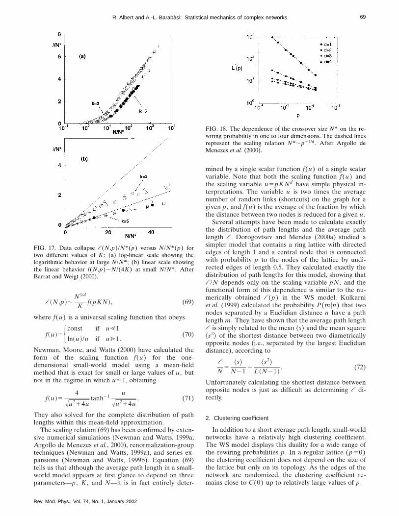
69R. Albert and A.-L. Barabasi: Statistical mechanics of complex networks
l ~N ,p !;N1/d
Kf~pKN !, (69)
where f(u) is a universal scaling function that obeys
f~u !5H const if u!1
ln~u !/u if u@1.(70)
Newman, Moore, and Watts (2000) have calculated theform of the scaling function f(u) for the one-dimensional small-world model using a mean-fieldmethod that is exact for small or large values of u , butnot in the regime in which u.1, obtaining
f~u !54
Au214utanh21
u
Au214u. (71)
They also solved for the complete distribution of pathlengths within this mean-field approximation.
The scaling relation (69) has been confirmed by exten-sive numerical simulations (Newman and Watts, 1999a;Argollo de Menezes et al., 2000), renormalization-grouptechniques (Newman and Watts, 1999a), and series ex-pansions (Newman and Watts, 1999b). Equation (69)tells us that although the average path length in a small-world model appears at first glance to depend on threeparameters—p , K , and N—it is in fact entirely deter-
FIG. 17. Data collapse l (N ,p)/N* (p) versus N/N* (p) fortwo different values of K : (a) log-linear scale showing thelogarithmic behavior at large N/N* ; (b) linear scale showingthe linear behavior l(N ,p);N/(4K) at small N/N* . AfterBarrat and Weigt (2000).
Rev. Mod. Phys., Vol. 74, No. 1, January 2002
mined by a single scalar function f(u) of a single scalarvariable. Note that both the scaling function f(u) andthe scaling variable u5pKNd have simple physical in-terpretations. The variable u is two times the averagenumber of random links (shortcuts) on the graph for agiven p , and f(u) is the average of the fraction by whichthe distance between two nodes is reduced for a given u .
Several attempts have been made to calculate exactlythe distribution of path lengths and the average pathlength l . Dorogovtsev and Mendes (2000a) studied asimpler model that contains a ring lattice with directededges of length 1 and a central node that is connectedwith probability p to the nodes of the lattice by undi-rected edges of length 0.5. They calculated exactly thedistribution of path lengths for this model, showing thatl /N depends only on the scaling variable pN , and thefunctional form of this dependence is similar to the nu-merically obtained l (p) in the WS model. Kulkarniet al. (1999) calculated the probability P(mun) that twonodes separated by a Euclidian distance n have a pathlength m . They have shown that the average path lengthl is simply related to the mean ^s& and the mean square^s2& of the shortest distance between two diametricallyopposite nodes (i.e., separated by the largest Euclidiandistance), according to
l
N5
^s&N21
2^s2&
L~N21 !. (72)
Unfortunately calculating the shortest distance betweenopposite nodes is just as difficult as determining l di-rectly.
2. Clustering coefficient
In addition to a short average path length, small-worldnetworks have a relatively high clustering coefficient.The WS model displays this duality for a wide range ofthe rewiring probabilities p . In a regular lattice (p50)the clustering coefficient does not depend on the size ofthe lattice but only on its topology. As the edges of thenetwork are randomized, the clustering coefficient re-mains close to C(0) up to relatively large values of p .
FIG. 18. The dependence of the crossover size N* on the re-wiring probability in one to four dimensions. The dashed linesrepresent the scaling relation N* ;p21/d. After Argollo deMenezes et al. (2000).

70 R. Albert and A.-L. Barabasi: Statistical mechanics of complex networks
The dependence of C(p) on p can be derived using aslightly different but equivalent definition of C , intro-duced by Barrat and Weigt (2000). According to thisdefinition, C8(p) is the fraction between the mean num-ber of edges between the neighbors of a node and themean number of possible edges between those neigh-bors. In a more graphic formulation (Newman, Strogatz,and Watts, 2001),
C8533number of triangles
number of connected triples. (73)
Here triangles are trios of nodes in which each node isconnected to both of the others, and connected triplesare trios in which at least one is connected to both oth-ers, the factor 3 accounting for the fact that each trianglecontributes to three connected triples. This definitioncorresponds to the concept of the ‘‘fraction of transitivetriples’’ used in sociology (see Wasserman and Faust,1994).
To calculate C8(p) for the WS model, let us startwith a regular lattice with a clustering coefficient C(0).For p.0, two neighbors of a node i that were connectedat p50 are still neighbors of i and connected by anedge with probability (12p)3, since there are threeedges that need to remain intact. Consequently C8(p).C(0)(12p)3. Barrat and Weigt (2000) have verifiedthat the deviation of C(p) from this expression is smalland goes to zero as N→` . The corresponding expres-sion for the Newman-Watts model is (Newman, 2001e)
C8~p !53K~K21 !
2K~2K21 !18pK214p2K2 . (74)
3. Degree distribution
In the WS model for p50 each node has the samedegree K . Thus the degree distribution is a delta func-tion centered at K . A nonzero p introduces disorder inthe network, broadening the degree distribution whilemaintaining the average degree equal to K . Since only asingle end of every edge is rewired (pNK/2 edges intotal), each node has at least K/2 edges after the rewir-ing process. Consequently for K.2 there are no isolatednodes and the network is usually connected, unlike arandom graph which consists of isolated clusters for awide range of connection probabilities.
For p.0, the degree ki of a vertex i can be written as(Barrat and Weigt, 2000) ki5K/21ci , where ci can bedivided into two parts: ci
1<K/2 edges have been left inplace (with probability 12p), while ci
25ci2ci1 edges
have been rewired towards i , each with probability 1/N .The probability distributions of ci
1 and ci2 are
P1~ci1!5CK/2
ci1
~12p !ci1pK/22ci
1(75)
and
P2~ci2!5CpNK/2
ci2 S 1
N D ci2S 12
1N D pNK/22ci
2
.~pK/2!ci
2
ci2!
e2pK/2 (76)
Rev. Mod. Phys., Vol. 74, No. 1, January 2002
for large N . Combining these two factors, the degreedistribution follows
P~k !5 (n50
f(k ,K)
CK/2n ~12p !npK/22n
~pK/2!k2K/22n
~k2K/22n !!e2pK/2
(77)
for k>K/2, where f(k ,K)5min(k2K/2,K/2).The shape of the degree distribution is similar to that
of a random graph. It has a pronounced peak at ^k&5K and decays exponentially for large k (Fig. 19). Thusthe topology of the network is relatively homogeneous,all nodes having approximately the same number ofedges.
4. Spectral properties
As discussed in Sec. III.G, the spectral density r(l) ofa graph reveals important information about its topol-ogy. Specifically, we have seen that for large randomgraphs r(l) converges to a semicircle. It comes as nosurprise that the spectrum of the Watts-Strogatz modeldepends on the rewiring probability p (Farkas et al.,2001). For p50 the network is regular and periodical;consequently r(l) contains numerous singularities [Fig.20(a)]. For intermediate values of p these singularitiesbecome blurred, but r(l) retains a strong skewness[Figs. 20(b) and (c)]. Finally, as p→1, r(l) approachesthe semicircle law characterizing random graphs [Fig.20(d)]. While the details of the spectral density changeconsiderably with p , the third moment of r(l) is con-sistently high, indicating a high number of triangles inthe network. Thus the results summarized in Fig. 20 al-low us to conclude that a high number of triangles is abasic property of the WS model (see also Gleis et al.,2000). The high regularity of small-world models for a
FIG. 19. Degree distribution of the Watts-Strogatz model forK53 and various p . We can see that only k>K/2 values arepresent, and the mean degree is ^k&5K . The symbols are ob-tained from numerical simulations of the Watts-Strogatz modelwith N51000, and the lines correspond to Eq. (77). As a com-parison, the degree distribution of a random graph with thesame parameters is plotted with filled symbols. After Barratand Weigt (2000).
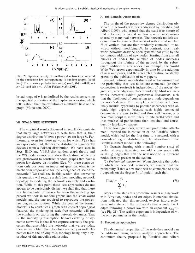
71R. Albert and A.-L. Barabasi: Statistical mechanics of complex networks
broad range of p is underlined by the results concerningthe spectral properties of the Laplacian operator, whichtell us about the time evolution of a diffusive field on thegraph (Monasson, 2000).
VII. SCALE-FREE NETWORKS
The empirical results discussed in Sec. II demonstratethat many large networks are scale free, that is, theirdegree distribution follows a power law for large k . Fur-thermore, even for those networks for which P(k) hasan exponential tail, the degree distribution significantlydeviates from a Poisson distribution. We have seen inSecs. III.D and VI.B.3 that random-graph theory andthe WS model cannot reproduce this feature. While it isstraightforward to construct random graphs that have apower-law degree distribution (Sec. V), these construc-tions only postpone an important question: what is themechanism responsible for the emergence of scale-freenetworks? We shall see in this section that answeringthis question will require a shift from modeling networktopology to modeling the network assembly and evolu-tion. While at this point these two approaches do notappear to be particularly distinct, we shall find that thereis a fundamental difference between the modeling ap-proach we took in random graphs and the small-worldmodels, and the one required to reproduce the power-law degree distribution. While the goal of the formermodels is to construct a graph with correct topologicalfeatures, the modeling of scale-free networks will putthe emphasis on capturing the network dynamics. Thatis, the underlying assumption behind evolving or dy-namic networks is that if we capture correctly the pro-cesses that assembled the networks that we see today,then we will obtain their topology correctly as well. Dy-namics takes the driving role, topology being only a by-product of this modeling philosophy.
FIG. 20. Spectral density of small-world networks, comparedto the semicircle law corresponding to random graphs (solidline). The rewiring probabilities are (a) p50; (b) p50.01; (c)p50.3; and (d) p51. After Farkas et al. (2001).
Rev. Mod. Phys., Vol. 74, No. 1, January 2002
A. The Barabasi-Albert model
The origin of the power-law degree distribution ob-served in networks was first addressed by Barabasi andAlbert (1999), who argued that the scale-free nature ofreal networks is rooted in two generic mechanismsshared by many real networks. The network models dis-cussed thus far assume that we start with a fixed numberN of vertices that are then randomly connected or re-wired, without modifying N . In contrast, most real-world networks describe open systems that grow by thecontinuous addition of new nodes. Starting from a smallnucleus of nodes, the number of nodes increasesthroughout the lifetime of the network by the subse-quent addition of new nodes. For example, the WorldWide Web grows exponentially in time by the additionof new web pages, and the research literature constantlygrows by the publication of new papers.
Second, network models discussed so far assume thatthe probability that two nodes are connected (or theirconnection is rewired) is independent of the nodes’ de-gree, i.e., new edges are placed randomly. Most real net-works, however, exhibit preferential attachment, suchthat the likelihood of connecting to a node depends onthe node’s degree. For example, a web page will morelikely include hyperlinks to popular documents with al-ready high degrees, because such highly connecteddocuments are easy to find and thus well known, or anew manuscript is more likely to cite well-known andthus much-cited publications than less-cited and conse-quently less-known papers.
These two ingredients, growth and preferential attach-ment, inspired the introduction of the Barabasi-Albertmodel, which led for the first time to a network with apower-law degree distribution. The algorithm of theBarabasi-Albert model is the following:
(1) Growth: Starting with a small number (m0) ofnodes, at every time step, we add a new node withm(<m0) edges that link the new node to m differentnodes already present in the system.
(2) Preferential attachment: When choosing the nodesto which the new node connects, we assume that theprobability P that a new node will be connected to nodei depends on the degree ki of node i , such that
P~ki!5ki
(j
kj
. (78)
After t time steps this procedure results in a networkwith N5t1m0 nodes and mt edges. Numerical simula-tions indicated that this network evolves into a scale-invariant state with the probability that a node has kedges following a power law with an exponent gBA53(see Fig. 21). The scaling exponent is independent of m ,the only parameter in the model.
B. Theoretical approaches
The dynamical properties of the scale-free model canbe addressed using various analytic approaches. Thecontinuum theory proposed by Barabasi and Albert

72 R. Albert and A.-L. Barabasi: Statistical mechanics of complex networks
FIG. 21. Numerical simulations of network evolution: (a) Degree distribution of the Barabasi-Albert model, with N5m01t5300 000 and s, m05m51; h, m05m53; L, m05m55; and n, m05m57. The slope of the dashed line is g52.9, providingthe best fit to the data. The inset shows the rescaled distribution (see text) P(k)/2m2 for the same values of m , the slope of thedashed line being g53; (b) P(k) for m05m55 and various system sizes, s, N5100 000; h, N5150 000; L, N5200 000. Theinset shows the time evolution for the degree of two vertices, added to the system at t155 and t2595. Here m05m55, and thedashed line has slope 0.5, as predicted by Eq. (81). After Barabasi, Albert, and Jeong (1999).
(1999) focuses on the dynamics of node degrees, fol-lowed by the master-equation approach of Dorogovtsev,Mendes, and Samukhin (2000a) and the rate-equationapproach introduced by Krapivsky, Redner, and Leyvraz(2000). As these methods are often used interchange-ably in the subsequent section, we briefly review each ofthem.
Continuum theory: The continuum approach intro-duced by Barabasi and Albert (1999) and Barabasi, Al-bert, and Jeong (1999) calculates the time dependenceof the degree ki of a given node i . This degree will in-crease every time a new node enters the system andlinks to node i , the probability of this process beingP(ki). Assuming that ki is a continuous real variable,the rate at which ki changes is expected to be propor-tional to P(ki). Consequently ki satisfies the dynamicalequation
]ki
]t5mP~ki!5m
ki
(j51
N21
kj
. (79)
The sum in the denominator goes over all nodes in thesystem except the newly introduced one; thus its value is( jkj52mt2m , leading to
]ki
]t5
ki
2t. (80)
The solution of this equation, with the initial conditionthat every node i at its introduction has ki(t i)5m , is
Rev. Mod. Phys., Vol. 74, No. 1, January 2002
ki~ t !5mS t
t iD b
with b512
. (81)
Equation (81) indicates that the degree of all nodesevolves the same way, following a power law, the onlydifference being the intercept of the power law.
Using Eq. (81), one can write the probability that anode has a degree ki(t) smaller than k , P@ki(t),k# , as
P@ki~ t !,k#5PS t i.m1/bt
k1/b D . (82)
Assuming that we add the nodes at equal time intervalsto the network, the t i values have a constant probabilitydensity
P~ t i!51
m01t. (83)
Substituting this into Eq. (82) we obtain
PS t i.m1/bt
k1/b D512m1/bt
k1/b~ t1m0!. (84)
The degree distribution P(k) can be obtained using
P~k !5]P@ki~ t !,k#
]k5
2m1/bt
m01t
1k1/b11 , (85)
predicting that asymptotically (t→`)
P~k !;2m1/bk2g with g51b
1153 (86)
being independent of m , in agreement with the numeri-cal results.

73R. Albert and A.-L. Barabasi: Statistical mechanics of complex networks
As the power law observed for real networks de-scribes systems of rather different sizes, it is expectedthat a correct model should provide a time-independentdegree distribution. Indeed, Eq. (85) predicts that as-ymptotically the degree distribution of the Barabasi-Albert model is independent of time (and subsequentlyindependent of the system size N5m01t), indicatingthat, despite its continuous growth, the network reachesa stationary scale-free state. Furthermore, Eq. (85) alsoindicates that the coefficient of the power-law distribu-tion is proportional to m2. All these predictions are con-firmed by numerical simulations (see Fig. 21).
Master-equation approach: The method introduced byDorogovtsev, Mendes, and Samukhin (2000a; see alsoKullmann and Kertesz, 2001) studies the probabilityp(k ,t i ,t) that at time t a node i introduced at time t i hasa degree k . In the Barabasi-Albert model, when a newnode with m edges enters the system, the degree of nodei increases by 1 with a probability mP(k)5k/2t ; other-wise it stays the same. Consequently the master equa-tion governing p(k ,t i ,t) for the Barabasi-Albert modelhas the form
p~k ,t i ,t11 !5k21
2tp~k21,t i ,t !1S 12
k
2t Dp~k ,t i ,t !.
(87)
The degree distribution can be obtained as
P~k !5 limt→`
S (t i
p~k ,t i ,t ! D Y t . (88)
Equation (87) implies that P(k) is the solution of therecursive equation
P~k !5H k21k12
P~k21 ! for k>m11
2/~m12 ! for k5m ,(89)
giving
P~k !52m~m11 !
k~k11 !~k12 !, (90)
very close to Eq. (86) obtained using the continuumtheory.
Rate-equation approach: The rate-equation approach,introduced by Krapivsky, Redner, and Leyvraz (2000),focuses on the average number Nk(t) of nodes with kedges at time t . When a new node enters the network inthe scale-free model, Nk(t) changes as
dNk
dt5m
~k21 !Nk21~ t !2kNk~ t !
(k
kNk~ t !1dk ,m . (91)
Here the first term accounts for the new edges that con-nect to nodes with k21 edges, thus increasing their de-gree to k . The second term describes the new edgesconnecting to nodes with k edges turning them intonodes with k11 edges, decreasing the number of nodeswith k edges. The third term accounts for the new nodeswith m edges. In the asymptotic limit Nk(t)5tP(k) and
Rev. Mod. Phys., Vol. 74, No. 1, January 2002
(kkNk(t)52mt , leading to the same recursive equation(89), as predicted by the master-equation approach.
The master-equation and rate-equation approachesare completely equivalent and offer the same asymptoticresults as the continuum theory. Thus for calculating thescaling behavior of the degree distribution they can beused interchangeably. In addition, these methods, notusing a continuum assumption, appear more suitable forobtaining exact results in more challenging networkmodels.
C. Limiting cases of the Barabasi-Albert model
The power-law scaling in the Barabasi-Albert modelindicates that growth and preferential attachment playimportant roles in network development. But are bothof them necessary for the emergence of power-law scal-ing? To address this question, two limiting cases of theBarabasi-Albert model have been investigated, whichcontain only one of these two mechanisms (Barabasiand Albert, 1999; Barabasi, Albert, and Jeong, 1999).
Model A keeps the growing character of the networkwithout preferential attachment. Starting with a smallnumber of nodes (m0), at every time step we add a newnode with m(<m0) edges. We assume that the newnode connects with equal probability to the nodes al-ready present in the system, i.e., P(ki)51/(m01t21),independent of ki .
The continuum theory predicts that ki(t) follows alogarithmic time dependence, and for t→` the degreedistribution decays exponentially, following [Fig. 22(a)]
P~k !5e
mexpS 2
k
m D . (92)
The exponential character of the distribution indicatesthat the absence of preferential attachment eliminatesthe scale-free character of the resulting network.
Model B starts with N nodes and no edges. At eachtime step a node is selected randomly and connectedwith probability P(ki)5ki /( jkj to a node i in the sys-tem. Consequently model B eliminates the growth pro-cess, the number of nodes being kept constant duringthe network evolution. Numerical simulations indicatethat while at early times the model exhibits power-lawscaling, P(k) is not stationary (Fig. 22). Since N is con-stant and the number of edges increases with time, afterT.N2 time steps the system reaches a state in which allnodes are connected.
The time evolution of the individual degrees can becalculated analytically using the continuum theory, indi-cating that
ki~ t !.2N
t , (93)
assuming N@1, in agreement with the numerical results[Fig. 22(b)].
Since the continuum theory predicts that after a tran-sient period the average degree of all nodes should havethe same value given by Eq. (93), we expect that the

74 R. Albert and A.-L. Barabasi: Statistical mechanics of complex networks
FIG. 22. Degree distributionfor two models: (a) Degree dis-tribution for model A: s, m05m51; h, m05m53; L, m05m55; n, m05m57. The sizeof the network is N5800 000.Inset: time evolution for the de-gree of two vertices added tothe system at t157 and t2597.Here m05m53. The dashedline follows ki(t)5mln(m01t21); (b) the degree distributionfor model B for N510 000: s,t5N ; h, t55N ; and L, t540N . Inset: time dependenceof the degrees of two vertices.The system size is N510 000.After Barabasi, Albert, andJeong (1999).
degree distribution becomes a Gaussian around its meanvalue. Indeed, Fig. 22(b) shows that the shape of P(k)changes from the initial power law to a Gaussian.
Motivated by correlations between stocks in financialmarkets and airline route maps, a prior model incorpo-rating preferential attachment while keeping N constantwas independently proposed and studied by Amaralet al. (1999).
The failure of models A and B to lead to a scale-freedistribution indicates that growth and preferential at-tachment are needed simultaneously to reproduce thestationary power-law distribution observed in real net-works.
D. Properties of the Barabasi-Albert model
While the Barabasi-Albert model captures the power-law tail of the degree distribution, it has other propertiesthat may or may not agree with empirical results on realnetworks. As we discussed in Sec. I, a characteristic fea-ture of real networks is the coexistence of clustering andshort path lengths. Thus we need to investigate whetherthe network generated by the model has a small-worldcharacter.
1. Average path length
Figure 23 shows the average path length of aBarabasi-Albert network with average degree ^k&54 asa function of the network size N , compared with theaverage path length of a random graph with the samesize and average degree. The figure indicates that theaverage path length is smaller in the Barabasi-Albertnetwork than in a random graph for any N , indicatingthat the heterogeneous scale-free topology is more effi-cient in bringing the nodes close than is the homoge-neous topology of random graphs. We find that the av-erage path length of the Barabasi-Albert network
Rev. Mod. Phys., Vol. 74, No. 1, January 2002
increases approximately logarithmically with N , the bestfit following a generalized logarithmic form
l 5A ln~N2B !1C . (94)
Recent analytical results indicate that there is a doublelogarithmic correction to the logarithmic N dependence,i.e., l ;ln(N)/lnln(N) (Bollobas and Riordan, 2001).
In Fig. 23 we also show the prediction of Eq. (60) forthese networks, using the numerically determined num-ber of nearest and next-nearest neighbors. While the fitis good for the random graph, Eq. (60) systematicallyunderestimates the average path length of the Barabasi-
FIG. 23. Characteristic path length l versus network size N ina Barabasi-Albert (BA) network with ^k&54 (s), comparedwith a random graph of the same size and average degree gen-erated with the algorithm described in Sec. III.A (h). Thedashed line follows Eq. (94), and the solid lines represent Eq.(60) with z15^k& and z2 the numerically obtained number ofnext-nearest neighbors in the respective networks.

75R. Albert and A.-L. Barabasi: Statistical mechanics of complex networks
Albert network, as it does the average path length ofreal networks (see Table II, last three columns).
The failure of Eq. (60) underlies the fact that the to-pology of the network generated by the Barabasi-Albertmodel is different from the topology of a random net-work with power-law degree distribution (Sec. V). Thedynamical process that generates the network intro-duces nontrivial correlations that affect all topologicalproperties.
2. Node degree correlations
In random-graph models with arbitrary degree distri-bution (see Aiello et al., 2000 and Newman, Strogatz,and Watts, 2001), the node degrees are uncorrelated.Krapivsky and Redner (2001) have shown that in theBarabasi-Albert model correlations develop spontane-ously between the degrees of connected nodes.
Let us consider all node pairs with degree k and lconnected by an edge. Without loss of generality we as-sume that the node with degree k was added later to thesystem, implying that k,l since, according to Eq. (81),older nodes have higher degree than younger ones, andfor simplicity we use m51. Denoting by Nkl(t) thenumber of connected pairs of nodes with degree k and l ,we have
dNkl
dt5
~k21 !Nk21,l2kNkl
(k
kN~k !
1~ l21 !Nk ,l212lNkl
(k
kN~k !
1~ l21 !Nl21dk1 . (95)
The first term on the right-hand side accounts for thechange in Nkl due to the addition of an edge to a nodeof degree k21 or k that is connected to a node of de-gree l . Since the addition of a new edge increases thenode’s degree by 1, the first term in the numerator cor-responds to a gain in Nkl , while the second correspondsto a loss. The second term on the right-hand side incor-porates the same effects as the first applied to the othernode. The last term takes into account the possibilitythat k51; thus the edge that is added to the node withdegree l21 is the same edge that connects the twonodes.
This equation can be transformed into a time-independent recursion relation using the hypotheses(kkN(k)→2t and Nkl(t)→tnkl . Solving for nkl we ob-tain
nkl54~ l21 !
k~k11 !~k1l !~k1l11 !~k1l12 !
112~ l21 !
k~k1l21 !~k1l !~k1l11 !~k1l12 !. (96)
For a network with an arbitrary degree distribution, ifthe edges are placed randomly, nkl5nknl . The most im-portant feature of the result (96) is that the joint distri-bution does not factorize, i.e., nklÞnknl . This indicatesthe spontaneous appearance of correlations between the
Rev. Mod. Phys., Vol. 74, No. 1, January 2002
degrees of the connected nodes. The only case in whichnkl can be simplified to a factorized expression is when1!k!l , and nkl becomes
nkl.k22l22, (97)
but even then it is different from nkl5k23l23, as ex-pected if correlations are absent from the network. Thisresult offers the first explicit proof that the dynamicalprocess that creates a scale-free network builds up non-trivial correlations between the nodes that are notpresent in the uncorrelated models discussed in Sec. V.
3. Clustering coefficient
While the clustering coefficient has been much inves-tigated for the Watts-Strogatz model (Sec. VI.B.2), thereis no analytical prediction for the Barabasi-Albertmodel. Figure 24 shows the clustering coefficient of aBarabasi-Albert network with average degree ^k&54and different sizes, compared with the clustering coeffi-cient Crand5^k&/N of a random graph. We find that theclustering coefficient of the scale-free network is aboutfive times higher than that of the random graph, and thisfactor slowly increases with the number of nodes. How-ever, the clustering coefficient of the Barabasi-Albertmodel decreases with the network size, following ap-proximately a power law C;N20.75, which, while aslower decay than the C5^k&N21 decay observed forrandom graphs, is still different from the behavior of thesmall-world models, where C is independent of N .
4. Spectral properties
The spectral density of the Barabasi-Albert model iscontinuous, but it has a markedly different shape fromthe semicircular spectral density of random graphs (Far-kas et al., 2001; Goh, Kahng, and Kim, 2001). Numericalsimulations indicate that the bulk of r(l) has a triangle-like shape with the top lying well above the semicircleand edges decaying as a power law (Fig. 25). This power-
FIG. 24. Clustering coefficient versus size of the Barabasi-Albert (BA) model with ^k&54, compared with the clusteringcoefficient of a random graph, Crand.^k&/N .
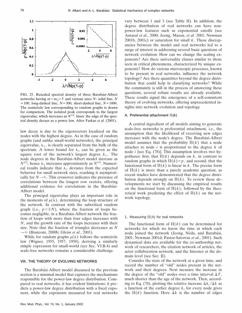
76 R. Albert and A.-L. Barabasi: Statistical mechanics of complex networks
law decay is due to the eigenvectors localized on thenodes with the highest degree. As in the case of randomgraphs (and unlike small-world networks), the principaleigenvalue, l1 , is clearly separated from the bulk of thespectrum. A lower bound for l1 can be given as thesquare root of the network’s largest degree k1 . Thenode degrees in the Barabasi-Albert model increase asN1/2; hence l1 increases approximately as N1/4. Numeri-cal results indicate that l1 deviates from the expectedbehavior for small network sizes, reaching it asymptoti-cally for N→` . This crossover indicates the presence ofcorrelations between the longest row vectors, offeringadditional evidence for correlations in the Barabasi-Albert model.
The principal eigenvalue plays an important role inthe moments of r(l), determining the loop structure ofthe network. In contrast with the subcritical randomgraph (i.e., p,1/N), where the fraction of loops be-comes negligible, in a Barabasi-Albert network the frac-tion of loops with more than four edges increases withN , and the growth rate of the loops increases with theirsize. Note that the fraction of triangles decreases as N→` (Bianconi, 2000b; Gleiss et al., 2001).
While for random graphs r(l) follows the semicirclelaw (Wigner, 1955, 1957, 1958), deriving a similarlysimple expression for small-world (see Sec. VI.B.4) andscale-free networks remains a considerable challenge.
VIII. THE THEORY OF EVOLVING NETWORKS
The Barabasi-Albert model discussed in the previoussection is a minimal model that captures the mechanismsresponsible for the power-law degree distribution. Com-pared to real networks, it has evident limitations: it pre-dicts a power-law degree distribution with a fixed expo-nent, while the exponents measured for real networks
FIG. 25. Rescaled spectral density of three Barabasi-Albertnetworks having m5m055 and various sizes N : solid line, N5100; long-dashed line, N5300; short-dashed line, N51000.The semicircle law corresponding to random graphs is drawnfor comparison. The isolated peak corresponds to the largesteigenvalue, which increases as N1/4. Inset: the edge of the spec-tral density decays as a power law. After Farkas et al. (2001).
Rev. Mod. Phys., Vol. 74, No. 1, January 2002
vary between 1 and 3 (see Table II). In addition, thedegree distribution of real networks can have non-power-law features such as exponential cutoffs (seeAmaral et al., 2000; Jeong, Mason, et al. 2001; Newman2001b, 2001c) or saturation for small k . These discrep-ancies between the model and real networks led to asurge of interest in addressing several basic questions ofnetwork evolution: How can we change the scaling ex-ponents? Are there universality classes similar to thoseseen in critical phenomena, characterized by unique ex-ponents? How do various microscopic processes, knownto be present in real networks, influence the networktopology? Are there quantities beyond the degree distri-bution that could help in classifying networks? Whilethe community is still in the process of answering thesequestions, several robust results are already available.These results signal the emergence of a self-consistenttheory of evolving networks, offering unprecedented in-sights into network evolution and topology.
A. Preferential attachment P(k)
A central ingredient of all models aiming to generatescale-free networks is preferential attachment, i.e., theassumption that the likelihood of receiving new edgesincreases with the node’s degree. The Barabasi-Albertmodel assumes that the probability P(k) that a nodeattaches to node i is proportional to the degree k ofnode i [see Eq. (78)]. This assumption involves two hy-potheses: first, that P(k) depends on k , in contrast torandom graphs in which P(k)5p , and second, that thefunctional form of P(k) is linear in k . The precise formof P(k) is more than a purely academic question, asrecent studies have demonstrated that the degree distri-bution depends strongly on P(k). To review these de-velopments we start by discussing the empirical resultson the functional form of P(k), followed by the theo-retical work predicting the effect of P(k) on the net-work topology.
1. Measuring P(k) for real networks
The functional form of P(k) can be determined fornetworks for which we know the time at which eachnode joined the network (Jeong, Neda, and Barabasi,2001; Newman 2001d; Pastor-Satorras et al., 2001). Suchdynamical data are available for the co-authorship net-work of researchers, the citation network of articles, theactor collaboration network, and the Internet at the do-main level (see Sec. II).
Consider the state of the network at a given time, andrecord the number of ‘‘old’’ nodes present in the net-work and their degrees. Next measure the increase inthe degree of the ‘‘old’’ nodes over a time interval DT ,much shorter than the age of the network. Then, accord-ing to Eq. (78), plotting the relative increase Dki /Dk asa function of the earlier degree ki for every node givesthe P(k) function. Here Dk is the number of edges

77R. Albert and A.-L. Barabasi: Statistical mechanics of complex networks
added to the network in the time DT . We can reducefluctuations in the data by plotting the cumulative distri-bution
k~k !5 (ki50
k
P~ki!. (98)
As Fig. 26 shows, the obtained P(k) supports the ex-istence of preferential attachment. Furthermore, it ap-pears that in each case P(k) follows a power law, i.e.,
P~k !;ka. (99)
In some cases, such as the Internet (Jeong, Neda, andBarabasi, 2001; Pastor-Satorras et al., 2001), the citationnetwork (Jeong, Neda, and Barabasi, 2001), Medline,and the Los Alamos archive (Newman, 2001d) we havea.1, i.e., P(k) depends linearly on k as assumed in theBarabasi-Albert model. For other networks the depen-dence is sublinear, with a50.860.1 for the neuroscienceco-authorship and the actor collaboration networks(Jeong, Neda, and Barabasi, 2001).
2. Nonlinear preferential attachment
The effect of a nonlinear P(k) on the network dy-namics and topology was explained by Krapivsky, Red-ner, and Leyvraz (2000). Replacing linear preferentialattachment [Eq. (78)] with Eq. (99) in a directed net-work model, Krapivsky, Redner, and Leyvraz calculate
FIG. 26. Cumulative preferential attachment for (a) the cita-tion network; (b) the Internet; (c) the neuroscience scientificcollaboration network; (d) the actor collaboration network. Inall panels the dashed line corresponds to linear preferentialattachment, and the solid line to no preferential attachment.After Jeong, Neda, and Barabasi (2001).
Rev. Mod. Phys., Vol. 74, No. 1, January 2002
the average number Nk(t) of nodes with k21 incomingedges at time t by the rate-equation approach (see Sec.VII.B). The time evolution of Nk(t) follows
dNk
dt5
1Ma
@~k21 !aNk212kaNk#1dk1 , (100)
where Ma(t)5(kaNk(t) is the ath moment of Nk(t).In Eq. (100) the first term accounts for new nodes thatconnect to nodes with k21 edges, thus increasing theirdegree to k . The second term describes new nodes con-necting to nodes with k edges, turning them into nodeswith k11 edges and hence decreasing the number ofnodes with k edges. The third term accounts for the con-tinuous introduction of new nodes with a single outgoingedge.
Depending on the value of a, distinct phases havebeen identified:
(a) Sublinear case (a,1): In this regime in the long-time limit Ma(t) satisfies Ma(t)5mt , with a pre-factor 1<m5m(a)<2. Substituting Ma(t) and Nkinto Eq. (100), we obtain the degree distribution
P~k!5m
ka )j51
k S11m
jaD21
. (101)
This product can be expanded in series, and theresult is a stretch exponential in which a new termarises whenever a decreases below 1/l , where l isan arbitrary positive integer.
(b) Superlinear preferential attachment (a.1): In thisregime Eq. (100) has no analytical solution, but itsdiscretized version can be used to determine recur-sively the leading behavior of each Nk as t→` . Fora.2 a ‘‘winner-takes-all’’ phenomenon emerges,such that almost all nodes have a single edge, con-necting them to a ‘‘gel’’ node that has the rest ofthe edges of the network. For 3/2,a,2 the num-ber of nodes with two edges grows as t22a, whilethe number of nodes with more than two edges isagain finite. Again, the rest of the edges belong tothe gel node. In general for (l11)/l,a,l/(l21)the number of nodes with more than l edges is fi-nite even in infinite systems, while Nk;tk2(k21)a
for k<l .
In conclusion, the analytical calculations of Krapivsky,Redner, and Leyvraz demonstrate that the scale-free na-ture of the network is destroyed for nonlinear preferen-tial attachment. The only case in which the topology ofthe network is scale free is that in which the preferentialattachment is asymptotically linear, i.e., P(ki);a`ki aski→` . In this case the rate equation leads to
P~k !;k2g with g511m
a`. (102)
This way the exponent of the degree distribution can betuned to any value between 2 and `.
3. Initial attractiveness
Another general feature of P(k) in real networks isthat P(0)Þ0, i.e., there is a nonzero probability that a
78 R. Albert and A.-L. Barabasi: Statistical mechanics of complex networks
new node attaches to an isolated node (Jeong, Neda,and Barabasi, 2001). Thus in general P(k) has the form
P~k !5A1ka, (103)
where A is the initial attractiveness of the node i (Dor-ogovtsev, Mendes, and Samukhin, 2000a). Indeed, if A50, a node that has k50 can never increase its connec-tivity according to Eq. (78). However, in real networksevery node has a finite chance to be ‘‘discovered’’ andlinked to, even if it has no edges to start with. Thus theparameter A describes the likelihood that an isolatednode will be discovered, such as a new article’s beingcited the first time.
Dorogovtsev, Mendes, and Samukhin (2000a) gave anexact solution for a class of growing network modelsusing the master-equation approach (see Sec. VII.B). Intheir model at every time step a new node is added tothe network, followed by the addition of m directededges pointing from any node in the network to prefer-entially chosen nodes. The probability that a node willreceive an incoming edge is proportional to the sum ofan initial attractiveness and the number of incomingedges, i.e., P(kin)5A1kin . The calculations indicatethat the degree distribution follows P(k);k2g with g521 A/m . Consequently initial attractiveness does notdestroy the scale-free nature of the degree distribution;it only changes the degree exponent. These results agreewith the conclusion of Krapivsky, Redner, and Leyvraz(2000), who find that the power law P(k) is preservedfor a shifted linear P(k), since the effect of the initialattractiveness diminishes as k→` . A generalization ofthe Dorogovtsev-Mendes-Samukhin model (Dorogovt-sev, Mendes, and Samukhin, 2000b) allows for the ran-dom distribution of nr edges and an initial degree n ofevery new node. These changes do not modify the as-ymptotically linear scaling of the preferential attach-ment; thus this model also gives a power-law degree dis-tribution with g521(nr1n1A)/m .
B. Growth
In the Barabasi-Albert model the number of nodesand edges increases linearly in time, and consequentlythe average degree of the network is constant. In thissection we discuss the effect of nonlinear growth rateson the network dynamics and topology.
1. Empirical results
The ability of networks to follow different growth pat-terns is supported by several recent measurements. Forexample, the average degree of the Internet in Novem-ber of 1997 was 3.42, but it increased to 3.96 by Decem-ber of 1998 (Faloutsos et al., 1999). Similarly, the WorldWide Web has increased its average degree from 7.22 to7.86 in the five months between the measurements ofBroder et al. (2000). The average degree of the co-authorship network of scientists has been found to con-tinuously increase over an eight-year period (Barabasiet al., 2001). Finally, comparison of metabolic networksof organisms of different sizes indicates that the average
Rev. Mod. Phys., Vol. 74, No. 1, January 2002
degree of the substrates increases approximately linearlywith the number of substrates involved in the metabo-lism (Jeong et al., 2000). The increase of the average de-gree indicates that in many real systems the number ofedges increases faster than the number of nodes, sup-porting the presence of a phenomenon called acceleratedgrowth.
2. Analytical results
Dorogovtsev and Mendes (2001a) studied analyticallythe effect of accelerated growth on the degree distribu-tion, generalizing the directed model with the asymptoti-cally linear preferential attachment of Dorogovtsev,Mendes, and Samukhin (2000a; see also Sec. VIII.A). Inthis model, at every step a new node is added to thenetwork, which receives n incoming edges from randomnodes in the system. Additionally c0tu new edges aredistributed, each of them being directed from a ran-domly selected node to a node with high incoming de-gree, with asymptotically linear preferential attachmentP(kin)}A1kin . The authors show that acceleratedgrowth, controlled by the exponent u, does not changethe scale-free nature of the degree distribution, but itmodifies the degree exponent, which now becomes
g5111
11u. (104)
While the model of Dorogovtsev and Mendes (2001a)is based on a directed network, Barabasi et al. (2001)discuss an undirected model motivated by measure-ments on the evolution of the co-authorship network. Inthe model new nodes are added to the system with aconstant rate, and these new nodes connect to b nodesalready in the system with preferential attachment
Pi5bki
(j
kj
. (105)
Additionally, at every time step a linearly increasingnumber of edges (constituting a fraction a of the nodesthat are present in the network) are distributed betweenthe nodes, the probability that an edge is added betweennodes i and j being
Pij5kikj
( 8s ,l
kskl
N~ t !a . (106)
Here N(t) is the number of nodes in the system andthe summation goes over all nonequal values of s and l .As a result of these two processes the average degree ofthe network increases linearly in time, following ^k&5at12b , in agreement with the measurements on thereal co-author network. The continuum theory predictsthat the time-dependent degree distribution displays acrossover at a critical degree,
kc5Ab2t~212at/b !3/2, (107)
79R. Albert and A.-L. Barabasi: Statistical mechanics of complex networks
such that for k!kc , P(k) follows a power law with ex-ponent g51.5 and for k@kc the exponent is g53. Thisresult explains the fast-decaying tail of the degree distri-butions measured by Newman (2001a), and it indicatesthat as time increases the scaling behavior with g51.5becomes increasingly visible. An equivalent model, pro-posed by Dorogovtsev and Mendes (2001c), was able toreproduce the two separate power-law regimes in thedistribution of word combinations (Ferrer i Cancho andSole, 2001).
C. Local events
The Barabasi-Albert model incorporates only onemechanism for network growth: the addition of newnodes that connect to the nodes already in the system. Inreal systems, however, a series of microscopic eventsshape the network evolution, including the addition orrewiring of new edges or the removal of nodes or edges.Lately several models have been proposed to investigatethe effect of selected processes on the scale-free natureof the degree distribution, offering a more realistic de-scription of various real networks. Any local change inthe network topology can be obtained through a combi-nation of four elementary processes: addition or re-moval of a node and addition or removal of an edge. Butin reality these events come jointly; for example, therewiring of an edge is a combination of an edge removaland addition. Next we briefly review several studies thataddress in general terms the effects of local events onnetwork topology.
1. Internal edges and rewiring
A model that incorporates new edges between exist-ing nodes and the rewiring of edges was discussed byAlbert and Barabasi (2000). Starting with m0 isolatednodes, at each time step we perform one of the followingthree operations:
(i) With probability p we add m(m<m0) new edges.One end of a new edge is selected randomly, theother with probability
P~ki!5ki11
(j
~kj11!
. (108)
(ii) With probability q we rewire m edges. For this werandomly select a node i and remove an edge l ijconnected to it, replacing it with a new edge l ij8that connects i with node j8 chosen with probabil-ity P(kj8) given by Eq. (108).
(iii) With probability 12p2q we add a new node.The new node has m new edges that with prob-ability P(ki) are connected to nodes i alreadypresent in the system.
In the continuum theory the growth rate of the degreeof a node i is given by
Rev. Mod. Phys., Vol. 74, No. 1, January 2002
]ki
]t5~p2q !m
1N
1mki11
(j
~kj11 !
. (109)
The first term on the right-hand side corresponds to therandom selection of node i as a starting point of a newedge (with probability p) or as the end point from whichan edge is disconnected (with probability q). The secondterm corresponds to the selection of node i as an endpoint of an edge with the preferential attachmentpresent in all three of the possible processes.
The solution of Eq. (109) has the form
ki~ t !5@A~p ,q ,m !1m11#S t
t iD 1/B(p ,q ,m)
2A~p ,q ,m !21, (110)
where
A~p ,q ,m !5~p2q !S 2m~12q !
12p2q11 D ,
B~p ,q ,m !52m~12q !112p2q
m. (111)
The corresponding degree distribution has the gener-alized power-law form
P~k !}@k1k~p ,q ,m !#2g(p ,q ,m), (112)
where k(p ,q ,m)5A(p ,q ,m)11 and g(p ,q ,m)5B(p ,q ,m)11.
Equation (112) is valid only when A(p ,q ,m)1m11.0, which, for fixed p and m , translates into q,qmax5min$12p,(12p1m)/(112m)%. Thus the (p ,q) phasediagram separates into two regions: For q,qmax the de-gree distribution is given by Eq. (112), following a gen-eralized power law. For q.qmax , however, Eq. (112) isnot valid, but numerical simulations indicate that P(k)approaches an exponential.
While a power-law tail is present in any point of thescale-free regime, for small k the probability saturates atP@k(p ,q ,m)# , a feature seen in many real networks[Figs. 3(b) and (d)]. In addition, the exponent g(p ,q ,m)characterizing the tail of P(k) for k@k(p ,q) changescontinuously with p , q , and m , predicting a range ofexponents between 2 and `. The realistic nature of P(k)was confirmed by successfully fitting it to the degree dis-tribution of the actor collaboration network (Albert andBarabasi, 2000).
2. Internal edges and edge removal
Dorogovtsev and Mendes (2000c) consider a class ofundirected models in which new edges are added be-tween old sites and existing edges can be removed. Inthe first variant of the model, called a developing net-work, c new edges are introduced at every time step,which connect two unconnected nodes i and j with aprobability proportional to the product of their degrees[as in Eq. (106)], an assumption confirmed by empiricalmeasurements on the co-authorship network (Barabasi

80 R. Albert and A.-L. Barabasi: Statistical mechanics of complex networks
et al., 2001). It is assumed that c can be tuned continu-ously, such that c.0 for a developing and c,0 for adecaying network. The continuum theory predicts thatthe rate of change of the node degrees has the form
]ki
]t5
ki~ t !
E0
tkj~ t !dtj
12c
ki~ t !F E0
tkj~ t !dtj2ki~ t !G
F E0
tkj~ t !dtjG 2
2E0
tkj
2~ t !dtj
,
(113)
where the summation over all nodes ( jkj has been ap-proximated by an integral over all introduction times t j .The first term on the right-hand side incorporates linearpreferential attachment, while the second term corre-sponds to the addition of c new edges. Every node canbe at either end of the new edge, and the probability ofa node i becoming an end of the new edge is propor-tional to the product of its degree ki and the sum of thedegrees kj of all other nodes. The normalization factor isthe sum of all products kikj with i different from j .
In the asymptotic limit the second term can be ne-glected compared with the first term in both the numera-tor and denominator, and Eq. (113) becomes
]ki
]t5~112c !
ki~ t !
E0
tkj~ t !dtj
, (114)
which predicts the dynamic exponent (81) as
b5112c
2~11c !(115)
and the degree exponent as
g5211
112c. (116)
The limiting cases of this developing network are c50when the familiar Barabasi-Albert values b51/2 and g53 are obtained, and c→` , when b→1 and g→2.
In the decaying network at every time step ucu edgesare removed randomly. The decrease in the node de-grees due to this process is proportional to their currentvalue, so Eq. (114) applies here as well, the only differ-ence being that now c,0. A more rigorous calculationaccounting for the fact that only existing edges can beremoved confirms that the end result is identical withEqs. (115) and (116), only with negative c . The limitingvalue of c is 21, since the rate of removal of edgescannot be higher than the rate of addition of new nodesand edges, leading to the limit exponents b→2` andg→` .
D. Growth constraints
For many real networks the nodes have a finite life-time (for example, in social networks) or a finite edgecapacity (Internet routers or nodes in the electricalpower grid). Recently several groups have addressed thedegree to which such constraints affect the degree distri-bution.
Rev. Mod. Phys., Vol. 74, No. 1, January 2002
1. Aging and cost
Amaral et al. (2000) suggested that while several net-works do show deviations from the power-law behavior,they are far from being random networks. For example,the degree distribution of the electric power grid ofsouthern California and of the neural network of theworm C. elegans is more consistent with a single-scaleexponential distribution. Other networks, like the ex-tended actor collaboration network, in which TV filmsand series are included, have a degree distribution inwhich power-law scaling is followed by an exponentialcutoff for large k . In all these examples there are con-straints limiting the addition of new edges. For example,the actors have a finite active period during which theyare able to collect new edges, while for the electricalpower grid or neural networks there are constraints onthe total number of edges a particular node can have,driven by economic, physical, or evolutionary reasons.Amaral et al. propose that in order to explain these de-viations from a pure power law we need to incorporate
FIG. 27. Deviation from a power law of the degree distribu-tion due to adding (a) age and (b) capacity constraints to theBarabasi-Albert model. The constraints result in cutoffs of thepower-law scaling. After Amaral et al. (2000).

81R. Albert and A.-L. Barabasi: Statistical mechanics of complex networks
aging and cost or capacity constraints. The model stud-ied by them evolves following growth and preferentialattachment, but when a node reaches a certain age (ag-ing) or has more than a critical number of edges (capac-ity constraints), new edges cannot connect to it. In bothcases numerical simulations indicate that while for smallk the degree distribution still follows a power law, forlarge k an exponential cutoff develops (Fig. 27).
2. Gradual aging
Dorogovtsev and Mendes (2000b) propose that insome systems the probability that a new node connectsto a node i is not only proportional to the degree ki ofnode i , but it also depends on its age, decaying as (t2t i)
2n, where n is a tunable parameter. Papers or actorsgradually lose their ability to attract more edges, themodel assuming that this phaseout follows a power law.The calculations predict that the degree distribution de-pends on the exponent n: power-law scaling is presentonly for n,1, and the degree exponent depends on n(Fig. 28). Moreover, when n.1 power-law scaling com-pletely disappears, the degree distribution approachingan exponential.
E. Competition in evolving networks
The Barabasi-Albert model assumes that all nodes in-crease their degree following a power-law time depen-dence with the same dynamic exponent b51/2 [Eq.(81)]. As a consequence, the oldest nodes have the high-est number of edges, since they had the longest lifetimeto accumulate them. However, numerous examples indi-
FIG. 28. The dependence of the degree exponent g on theaging exponent n in the model of Dorogovtsev and Mendes(2000b). The points are obtained from simulations, while thesolid line is the prediction of the continuum theory. After Dor-ogovtsev and Mendes (2000b).
Rev. Mod. Phys., Vol. 74, No. 1, January 2002
cate that in real networks a node’s degree and growthrate do not depend on age alone. For example, on theWorld Wide Web some documents acquire a large num-ber of edges in a very short time through a combinationof good content and marketing (Adamic and Huberman,2000), and some research papers acquire many more ci-tations than their peers. Several studies have offeredmodels that address this phenomenon.
1. Fitness model
Bianconi and Barabasi (2001a) argue that real net-works have a competitive aspect, as each node has anintrinsic ability to compete for edges at the expense ofother nodes. They propose a model in which each nodeis assigned a fitness parameter h i which does not changein time. Thus at every time step a new node j with afitness h j is added to the system, where h j is chosen froma distribution r(h). Each new node connects with medges to the nodes already in the network, and the prob-ability of connecting to a node i is proportional to thedegree and the fitness of node i ,
P i5h iki
(j
h jkj
. (117)
This generalized preferential attachment ensures thateven a relatively young node with a few edges can ac-quire edges at a high rate if it has a high fitness param-eter. The continuum theory predicts that the rate ofchange of the degree of node i is
]ki
]t5m
h iki
(k
h jkj
. (118)
Assuming that the time evolution of ki follows Eq.(81) with a fitness-dependent b(h),
kh i~ t ,t i!5mS t
t iD b(h i)
, (119)
the dynamic exponent satisfies
FIG. 29. Time dependence of the degree kh(t), for nodes withfitness h50.3, 0.6, and 0.9. Note that kh(t) follows a powerlaw in each case and the dynamic exponent b(h), given by theslope of k(t), increases with h. After Bianconi and Barabasi(2000a).

82 R. Albert and A.-L. Barabasi: Statistical mechanics of complex networks
b~h!5h
Cwith C5E r~h!
h
12b~h!dh . (120)
Thus b is described by a spectrum of values governedby the fitness distribution (Fig. 29). Equation (119) indi-cates that nodes with higher fitness increase their degreefaster than those with lower fitness. Thus the fitnessmodel allows for late but fit nodes to take a central rolein the network topology. The degree distribution of themodel is a weighted sum of different power laws,
P~k !;E r~h!C
h S m
k D C/h 11
, (121)
which depends on the choice of the fitness distribution(see Sec. VIII.G.2). For example, for a uniform fitnessdistribution Eq. (120) gives C51.255 and b(h)5h/1.255, and the degree distribution is
P~k !;k2C21
ln~k !, (122)
i.e., a power law with a logarithmic correction. The fit-ness model can be extended to incorporate additionalprocesses, such as internal edges, which affect the expo-nents, a problem studied by Ergun and Rodgers (2001).
2. Edge inheritance
A different mechanism that gives individuality to thenew nodes is proposed by Dorogovtsev, Mendes, andSamukhin (2000c). They build on the evolving directed-network algorithm introduced in their earlier paper(Dorogovtsev, Mendes, and Samukhin, 2000a), this timeassuming that the degree of the new nodes is not con-stant but depends on the state of the network at the timethe new node is added to the system. Specifically, everynew node is assumed to be an ‘‘heir’’ of a randomlychosen old node, and it inherits a fraction c of the oldnode’s incoming edges (i.e., a fraction c of the nodes thatpoint to the parent node will also point to the heir). Theparameter c is assumed to be distributed with a prob-ability density h(c).
The time-dependent degree distribution for uniformlydistributed c indicates that the fraction of nodes with noincoming edges increases and tends to 1 asymptotically.The distribution of nonzero incoming edges tends to adistribution
P~kin ,kinÞ0 !5d
kin&
ln~akin!, (123)
where d.0.174 and a.0.84.
F. Alternative mechanisms for preferential attachment
It is now established that highly connected nodes havebetter chances of acquiring new edges than their less-connected counterparts. The Barabasi-Albert model re-flects this fact by incorporating it explicitly through pref-erential attachment (78). But where does preferentialattachment come from? We do not yet have a universalanswer to this question, and there is a growing suspicion
Rev. Mod. Phys., Vol. 74, No. 1, January 2002
that the mechanisms responsible for preferential attach-ment are system dependent. However, recently severalpapers have offered promising proposals and modelsthat shed some light on this issue. The unifying theme ofthese models is that while a preferential attachment isnot explicitly introduced, the mechanisms used to placenodes and edges effectively induce one. The diversity ofthe proposals vividly illustrates the wide range of micro-scopic mechanisms that could effect the evolution ofgrowing networks and still lead to the observed scale-free topologies.
1. Copying mechanism
Motivated by the desire to explain the power-law de-gree distribution of the World Wide Web, Kleinberget al. (1999) and Kumar et al. (2000a, 2000b) assume thatnew Web pages dedicated to a certain topic copy linksfrom existing pages on the same topic. In this model, ateach time step a new node is added to the network,which connects to the rest of the nodes with a constantnumber of directed edges. At the same time a ‘‘proto-type’’ node is chosen randomly from the nodes alreadyin the system. The outgoing edges of the new node aredistributed in the following way: with probability p thedestination of the ith edge is selected randomly, andwith probability 12p it is taken to be the destination ofthe ith edge of the prototype node. This second processincreases the probability of high-degree nodes’ receivingnew incoming edges. In fact, since the prototype nodesare selected randomly, the probability that a Web pagewith degree k will receive a new hyperlink is propor-tional to (12p)k , indicating that the copying mecha-nism effectively amounts to a linear preferential attach-ment. Kumar et al. prove that the expectation of theincoming degree distribution is
P~kin!5k2(22p)/(12p); (124)
thus P(k) follows a power law with an exponent thatvaries between 2 (for p→0) and ` (for p→1).
2. Edge redirection
Although inspired by a different mechanism, thegrowing network with the redirection model of Krapiv-sky and Redner (2001) is mathematically equivalentwith the model of Kumar et al. (2000a, 2000b) discussedabove. In this model at every time step a new node isadded to the system and an earlier node i is selecteduniformly as a possible target for attachment. Withprobability 12r a directed edge from the new node to iis created; however, with probability r the edge is redi-rected to the ancestor node j of node i (i.e., the node atwhich i attached when it was first added to the network).
When the rate-equation approach (Sec. VII.B) is ap-plied, the number of nodes N(k) with degree k evolvesas

83R. Albert and A.-L. Barabasi: Statistical mechanics of complex networks
dN~k !
dt5dk11
12r
M0~Nk212Nk!1
r
M0@~k22 !Nk21
2~k21 !Nk# . (125)
The first term corresponds to nodes that are just addedto the network. The second term indicates the randomselection of a node to which the new node will attach.This process affects N(k) if this node has a degree k21 [in which case its degree will become k , increasingN(k)] or k [in which case N(k) decreases by one]. Thenormalization factor M0 is the sum of all degrees. Thethird term corresponds to the rewiring process. Since theinitial node is chosen uniformly, if redirection does oc-cur, the probability that a node with k21 preexistingedges will receive the redirected edge is proportional tok22, the number of preexisting incoming edges. Thusredirection also leads to a linear preferential attach-ment.
This rate equation is equivalent with Eq. (100) with anasymptotically linear attachment P(k);k2211/r .Thus this model leads to a power-law degree distributionwith degree exponent g5111/r , which can be tuned toany value larger than 2.
3. Walking on a network
The walking mechanism proposed by Vazquez (2000)was inspired by citation networks. Entering a new field,we are usually aware of a few important papers and fol-low the references included in these to find other rel-evant articles. This process is continued recursively, suchthat a manuscript will contain references to papers dis-covered this way. Vazquez formulates the correspondingnetwork algorithm in the following way: We start withan isolated node. At every time step a new node isadded that links with a directed edge to a randomly se-lected node, and then it follows the edges starting fromthis node and links to their end points with probabilityp . This last step is repeated starting from the nodes towhich connections were established, until no new targetnode is found. In fact, this algorithm is similar to thebreadth-first search used in determining the clusterstructure of a network, with the exception that not alledges are followed, but only a fraction equal to p . In thespecial case of p51 one can see that nodes of high de-gree will be more likely to acquire new incoming edges,leading to a preferential attachment P(k)5(11k)/N .Consequently, the degree distribution follows a powerlaw with g52. If p varies between 0 and 1, numericalsimulations indicate a phase transition: for p,pc.0.4the degree distribution decays exponentially, while forp.pc it has a power-law tail with g very close to 2, thevalue corresponding to p51. Thus, while the modeldoes not explicitly include preferential attachment, themechanism responsible for creation of the edges inducesone.
4. Attaching to edges
Perhaps the simplest model of a scale-free networkwithout explicit preferential attachment was proposed
Rev. Mod. Phys., Vol. 74, No. 1, January 2002
by Dorogovtsev, Mendes, and Samukhin (2001a). In thismodel at every time step a new node connects to bothends of a randomly selected edge. Consequently theprobability that a node will receive a new edge is di-rectly proportional to its degree; in other words, thismodel has exactly the same preferential attachment asthe Barabasi-Albert model. It readily follows that thedegree distribution has the same asymptotic form as theBarabasi-Albert model, i.e., P(k);k23.
The evolving network models presented in this sectionattempt to capture the mechanisms that govern the evo-lution of network topology (see Table III), guided by theinformation contained in the degree distribution. Less isknown, however, about the clustering coefficients ofthese models. Notable exceptions are the models ofBarabasi et al. (2001; see also Sec. VIII.B) and Dor-ogovtsev, Mendes, and Samukhin (2001a; see also Sec.VIII.F). The clustering coefficient of the model of Bara-basi et al. displays a complex behavior as the networkincreases, first decreasing, going through a minimum,then increasing again, while the model of Dorogovtsev,Mendes, and Samukhin (2000d) has a constantasymptotic clustering coefficient. These results suggestthat evolving network models can capture the high clus-tering coefficients of real networks.
G. Connection to other problems in statistical mechanics
The modeling of complex networks has offered fertileground for statistical mechanics. Indeed, many advancesin our understanding of the scaling properties of bothsmall-world and evolving networks have benefited fromconcepts ranging from critical phenomena to nucleationtheory and gelation. On the other hand, there appears tobe another close link between statistical mechanics andevolving networks: the continuum theories proposed topredict the degree distribution can be mapped, often ex-actly, onto some well-known problems investigated instatistical physics. In the following we shall discuss twosuch mappings, relating evolving networks to the Simonmodel (Simon, 1955; see Amaral et al., 2000; Bornholdtand Ebel, 2001) and to a Bose gas (Bianconi and Bara-basi, 2001b).
1. The Simon model
Aiming to account for the wide range of empiricaldistributions following a power law, such as the fre-quency of word occurrences (Zipf, 1949), the number ofarticles published by scientists (Lotka, 1926), the popu-lations of cities (Zipf, 1949), or the distribution of in-comes (Pareto, 1898), Simon (1955) proposed a class ofstochastic models that result in a power-law distributionfunction. The simplest variant of the Simon model, de-scribed in terms of word frequencies, has the followingalgorithm: Consider a book that is being written and hasreached a length of N words. Denote by fN(i) the num-ber of different words that each occurred exactly i timesin the text. Thus fN(1) denotes the number of differentwords that have occurred only once. The text is contin-
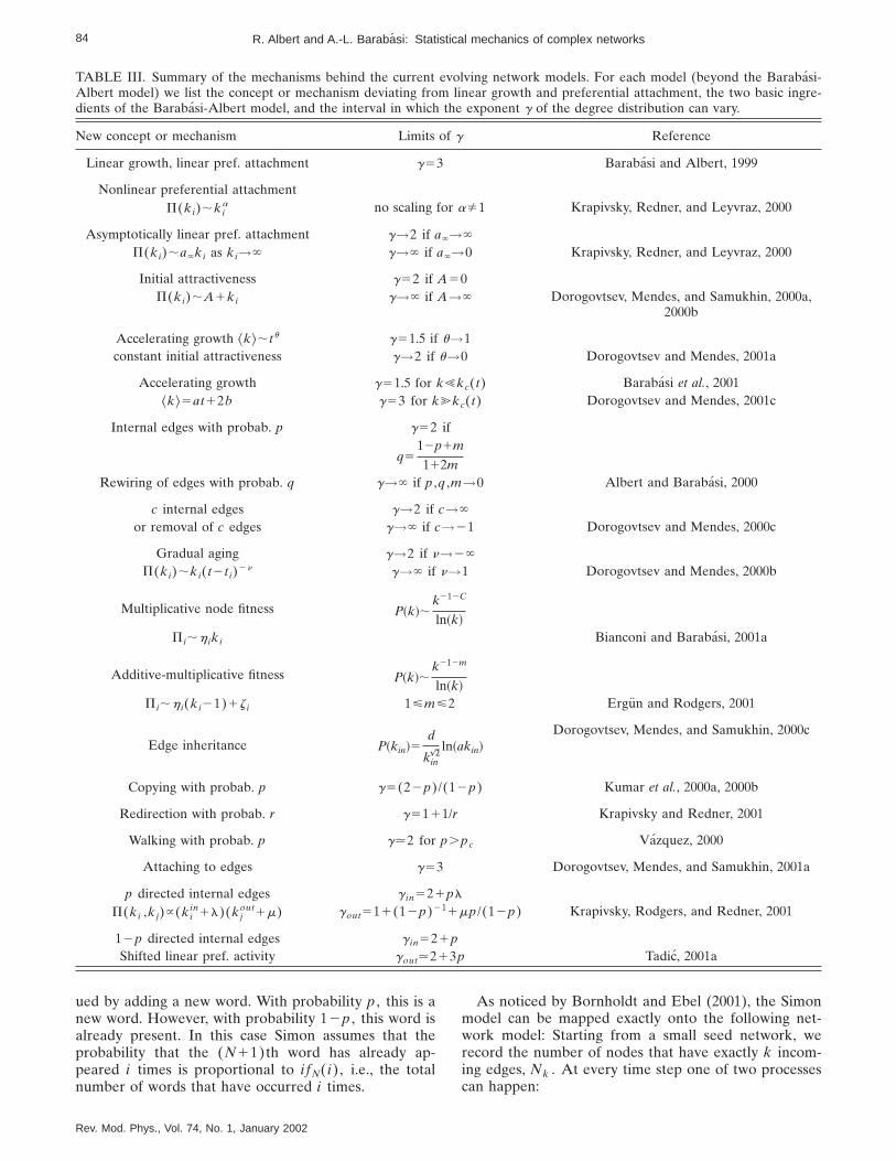
84 R. Albert and A.-L. Barabasi: Statistical mechanics of complex networks
TABLE III. Summary of the mechanisms behind the current evolving network models. For each model (beyond the Barabasi-Albert model) we list the concept or mechanism deviating from linear growth and preferential attachment, the two basic ingre-dients of the Barabasi-Albert model, and the interval in which the exponent g of the degree distribution can vary.
New concept or mechanism Limits of g Reference
Linear growth, linear pref. attachment g53 Barabasi and Albert, 1999
Nonlinear preferential attachmentP(ki);ki
a no scaling for aÞ1 Krapivsky, Redner, and Leyvraz, 2000
Asymptotically linear pref. attachment g→2 if a`→`
P(ki);a`ki as ki→` g→` if a`→0 Krapivsky, Redner, and Leyvraz, 2000
Initial attractiveness g52 if A50P(ki);A1ki g→` if A→` Dorogovtsev, Mendes, and Samukhin, 2000a,
2000b
Accelerating growth ^k&;tu g51.5 if u→1constant initial attractiveness g→2 if u→0 Dorogovtsev and Mendes, 2001a
Accelerating growth g51.5 for k!kc(t) Barabasi et al., 2001^k&5at12b g53 for k@kc(t) Dorogovtsev and Mendes, 2001c
Internal edges with probab. p g52 if
q512p1m
112mRewiring of edges with probab. q g→` if p ,q ,m→0 Albert and Barabasi, 2000
c internal edges g→2 if c→`
or removal of c edges g→` if c→21 Dorogovtsev and Mendes, 2000c
Gradual aging g→2 if n→2`
P(ki);ki(t2t i)2n g→` if n→1 Dorogovtsev and Mendes, 2000b
Multiplicative node fitness P~k!;k212C
ln~k!
P i;h iki Bianconi and Barabasi, 2001a
Additive-multiplicative fitness P~k!;k212m
ln~k!
P i;h i(ki21)1z i 1<m<2 Ergun and Rodgers, 2001
Edge inheritance P~kin!5d
kin&
ln~akin!Dorogovtsev, Mendes, and Samukhin, 2000c
Copying with probab. p g5(22p)/(12p) Kumar et al., 2000a, 2000b
Redirection with probab. r g5111/r Krapivsky and Redner, 2001
Walking with probab. p g.2 for p.pc Vazquez, 2000
Attaching to edges g53 Dorogovtsev, Mendes, and Samukhin, 2001a
p directed internal edges g in521pl
P(ki ,kj)}(kiin1l)(kj
out1m) gout511(12p)211mp/(12p) Krapivsky, Rodgers, and Redner, 2001
12p directed internal edges g in521pShifted linear pref. activity gout.213p Tadic, 2001a
ued by adding a new word. With probability p , this is anew word. However, with probability 12p , this word isalready present. In this case Simon assumes that theprobability that the (N11)th word has already ap-peared i times is proportional to ifN(i), i.e., the totalnumber of words that have occurred i times.
Rev. Mod. Phys., Vol. 74, No. 1, January 2002
As noticed by Bornholdt and Ebel (2001), the Simonmodel can be mapped exactly onto the following net-work model: Starting from a small seed network, werecord the number of nodes that have exactly k incom-ing edges, Nk . At every time step one of two processescan happen:

85R. Albert and A.-L. Barabasi: Statistical mechanics of complex networks
(a) With probability p a new node is added, and a ran-domly selected node will point to the new node.
(b) With probability 12p a directed edge between twoexisting nodes is added. The starting point of thisedge is selected randomly, while its end point isselected such that the probability that a node be-longing to the Nk nodes with k incoming edges willbe chosen is
P~class k !}kNk . (126)
To appreciate the nature of this mapping, we need toclarify several issues:
(1) While Eq. (126) represents a form of the ‘‘rich-get-richer’’ phenomenon, it does not imply preferentialattachment [Eq. (78)] as used in various evolvingnetwork models. However, Eq. (78) implies Eq.(126). Thus the Simon model describes a generalclass of stochastic processes that can result in apower-law distribution, appropriate to capturePareto and Zipf’s laws.
(2) The interest in evolving network models comes fromtheir ability to describe the topology of complex net-works. The Simon model does not have an underly-ing network structure, as it was designed to describeevents whose frequency follows a power law. Thusnetwork measures going beyond the degree distribu-tion, such as the average path length, spectral prop-erties, or clustering coefficient, cannot be obtainedfrom this mapping.
(3) The mapping described above leads to a directednetwork with internal edges, different from theBarabasi-Albert model. However, it is close to themodel proposed by Dorogovtsev, Mendes, and Sam-ukhin (2000a, 2000b) discussed in Sec. VIII.A.3,with the only difference being that here the initialattractiveness is present only for the isolated nodes.Since Eq. (126) corresponds to an asymptoticallylinear preferential attachment, a correspondencecan be made with the model of Krapivsky, Redner,and Leyvraz (2000) as well.
2. Bose-Einstein condensation
Bianconi and Barabasi (2001b) show the existence ofa close link between evolving networks and an equilib-rium Bose gas. Starting with the fitness model intro-duced in Sec. VIII.E.1, the mapping to a Bose gas can bedone by assigning an energy e i to each node, determinedby its fitness through the relation
e i521b
ln h i , (127)
where b51/T plays the role of inverse temperature. Anedge between two nodes i and j , having energies e i ande j , corresponds to two noninteracting particles, one oneach energy level (see Fig. 30). Adding a new node l tothe network corresponds to adding a new energy level e land 2m new particles to the system. Half of these par-ticles are deposited on the level e l (since all new edges
Rev. Mod. Phys., Vol. 74, No. 1, January 2002
start from the new node), while the other half are dis-tributed between the energy levels of the end points ofthe new edges, the probability that a particle lands onlevel i being given by
P i5e2be iki
( e2be iki
. (128)
The continuum theory predicts that the rate at whichparticles accumulate on energy level e i is given by
]ki~e i ,t ,t i!
]t5m
e2be iki~e i ,t ,t i!
Zt, (129)
where ki(e i ,t ,t i) is the occupation number of level i andZt is the partition function, defined as Zt5( j51te2be jkj(e j ,t ,t j). The solution of Eq. (129) is
ki~e i ,t ,t i!5mS t
t iD f(e i)
, (130)
where the dynamic exponent f(e) satisfies f(e)5e2b(e2m), m plays the role of the chemical potential,satisfying the equation
FIG. 30. Fitness and mapping between the network model andthe Bose gas: (a) On the left we have a network of five nodes,each characterized by a fitness h i . Equation (127) assigns anenergy e i to each h i (right). An edge from node i to node jcorresponds to a particle at level e i and one at e j . The networkevolves by adding a new node (dashed circle, h6), which con-nects to m52 other nodes (dashed lines), chosen following Eq.(78). In the gas this results in the addition of a new energylevel (e6 , dashed) populated by m52 new particles (s), andthe deposition of m52 other particles to energy levels towhich the new node is connected (e2 and e5). (b) In the fit-get-rich (FGR) phase we have a continuous degree distribu-tion, the several high-degree nodes linking the low-degreenodes together. In the energy diagram this corresponds to adecreasing occupation number with increasing energy. (c) Inthe Bose-Einstein condensate the fittest node attracts a finitefraction of all edges, corresponding to a highly populatedground level and sparsely populated higher energies. After Bi-anconi and Barabasi (2001b).

86 R. Albert and A.-L. Barabasi: Statistical mechanics of complex networks
E deg~e!1
eb(e2m)2151, (131)
and deg(e) is the degeneracy of the energy level e.Equation (131) suggests that in the t→` limit the occu-pation number, giving the number of particles with en-ergy e, follows the familiar Bose statistics
n~e!51
eb(e2m)21. (132)
The existence of the solution (130) depends on thefunctional form of the distribution g(e) of the energylevels, determined by the r(h) fitness distribution (seeSec. VIII.E.1). Specifically, if Eq. (131) has no non-negative solution for a given g(e) and b, we can observea Bose-Einstein condensation, indicating that a finitefraction of the particles condens on the lowest energylevel [see Fig. 30(c)].
This mapping to a Bose gas predicts the existence oftwo distinct phases as a function of the energy distribu-tion. In the fit-get-rich phase, describing the case of uni-form fitness discussed in Sec. VIII.E.1, the fitter nodesacquire edges at a higher rate than older but less fitnodes. In the end the fittest node will have the mostedges, but the richest node is not an absolute winner,since its share of the edges (i.e., the ratio of its edges andthe total number of edges in the network) decays to zerofor large system sizes [Fig. 30(b)]. The unexpected out-come of this mapping is the possibility of Bose-Einsteincondensation for T,TBE , when the fittest node ac-quires a finite fraction of the edges and maintains thisshare of edges over time [Fig. 30(c)]. A representativefitness distribution that leads to condensation is r(h)5(12h)l with l.1.
The temperature in Eq. (127) plays the role of adummy variable, since if we define a fixed distributionr(h), the existence of Bose-Einstein condensation orthe fit-get-rich phase depends only on the functionalform of r(h) and is independent of b. Indeed, b falls outat the end from all topologically relevant quantities. AsDorogovtsev and Mendes (2001b) have subsequentlyshown, the existence of Bose-Einstein condensation canbe derived directly from the fitness model, without em-ploying the mapping to a Bose gas. While the condensa-tion phenomenon appears to be similar to the gelationprocess observed by Krapivsky, Redner, and Leyvraz,(2000) in the case of superlinear preferential attach-ment, it is not clear at this point if this similarity ispurely accidental or if there is a deeper connection be-tween the fitness model and the fitness-free superlinearmodel.
IX. ERROR AND ATTACK TOLERANCE
Many complex systems display a surprising degree oftolerance for errors (Albert, Jeong, and Barabasi, 2000).For example, relatively simple organisms grow, persist,and reproduce despite drastic pharmaceutical or envi-ronmental interventions, an error tolerance attributed tothe robustness of the underlying metabolic and genetic
Rev. Mod. Phys., Vol. 74, No. 1, January 2002
network (Jeong et al., 2000; Jeong, Mason, et al., 2001).Complex communication networks display a high degreeof robustness: while key components regularly malfunc-tion, local failures rarely lead to loss of the globalinformation-carrying ability of the network. The stabilityof these and other complex systems is often attributed tothe redundant wiring of their underlying network struc-ture. But could the network topology, beyond redun-dancy, play a role in the error tolerance of such complexsystems?
While error tolerance and robustness almost alwayshave a dynamical component, here we shall focus onlyon the topological aspects of robustness, caused by edgeand/or node removal. The first results regarding networkreliability when subjected to edge removal came fromrandom-graph theory (Moore and Shannon, 1956a,1956b; Margulis, 1974; Bollobas, 1985). Consider an ar-bitrary connected graph HN of N nodes, and assumethat a p fraction of the edges have been removed. Whatis the probability that the resulting subgraph is con-nected, and how does it depend on the removal prob-ability p? For a broad class of starting graphs HN (Mar-gulis, 1974) there exists a threshold probability pc(N)such that if p,pc(N) the subgraph is connected, but ifp.pc(N) it is disconnected. This phenomenon is in factan inverse bond percolation problem defined on a graph,with the slight difference (already encountered in theevolution of a random graph) that the critical probabil-ity depends on N .
As the removal of a node implies the malfunctioningof all of its edges as well, node removal inflicts moredamage than edge removal. Does a threshold phenom-enon appear for node removal too? And to what degreedoes the topology of the network determine the net-work’s robustness? In the following we shall call a net-work error tolerant (or robust) if it contains a giant clus-ter comprised of most of the nodes even after a fractionof its nodes are removed. The results indicate a strongcorrelation between robustness and network topology.In particular, scale-free networks are more robust thanrandom networks against random node failures, but aremore vulnerable when the most connected nodes aretargeted (Albert, Jeong, and Barabasi, 2000).
A. Numerical results
In the first study comparing the robustness of theErdos-Renyi random graph and a scale-free networkgenerated by the Barabasi-Albert model, Albert, Jeong,and Barabasi (2000) investigated networks that have thesame number of nodes and edges, differing only in thedegree distribution. Two types of node removal wereconsidered. Random perturbations can cause the failureof some nodes; thus the first mechanism studied was theremoval of randomly selected nodes. The second mecha-nism, in which the most highly connected nodes are re-moved at each step, was selected because it is the mostdamaging to the integrity of the system. This secondchoice emulates an intentional attack on the network.

87R. Albert and A.-L. Barabasi: Statistical mechanics of complex networks
Let us start from a connected network, and at eachtime step remove a node. The disappearance of the nodeimplies the removal of all edges that connect to it, dis-rupting some of the paths between the remaining nodes(Fig. 31). One way to monitor the disruption of an ini-tially connected network is to study the relative size ofthe largest cluster that remains connected, S , and theaverage path length l of this cluster, as a function of thefraction f of the nodes removed from the system. Weexpect that the size of the largest cluster will decreaseand its average path length increase as an increasingnumber of nodes are removed from the network.
1. Random network, random node removal
We start by investigating the response of a randomnetwork to the random removal of its nodes [see Fig.
FIG. 31. Illustration of the effects of node removal on an ini-tially connected network. In the unperturbed state the distancebetween nodes A and B is 2, but after two nodes are removedfrom the system, it increases to 6. At the same time the net-work breaks into five isolated clusters.
FIG. 32. The relative size S (a),(b) and average path length l
(c),(d) of the largest cluster in an initially connected networkwhen a fraction f of the nodes are removed. (a),(c) Erdos-Renyi random network with N510 000 and ^k&54; (b),(d)scale-free network generated by the Barabasi-Albert modelwith N510 000 and ^k&54. h, random node removal; s, pref-erential removal of the most connected nodes. After Albert,Jeong, and Barabasi (2000).
Rev. Mod. Phys., Vol. 74, No. 1, January 2002
32(a), h], looking at the changes in the relative size ofthe largest cluster S (i.e., the fraction of nodes containedin the largest cluster) and its average path length l as anincreasing number of nodes are randomly removed.
As expected, for a random network, the size S of thelargest cluster decreases from S51 as f increases. If onlythe removed nodes were missing from the largest cluster,S would follow the diagonal corresponding to S51 forf50 and S50 for f51. While for small f , S follows thisline, as f increases the decrease becomes more rapid,indicating that clusters of nodes become isolated fromthe main cluster. At a critical fraction fc , S drops to 0,indicating that the network breaks into tiny isolatedclusters. These numerical results indicate an inverse per-colation transition. Indeed, percolation theory can beused to calculate the critical fraction fc (Sec. IX.B).
The behavior of the average path length l also con-firms this percolationlike transition: it starts from a valuecharacteristic of an unperturbed random graph, in-creases with f as paths are disrupted in the network, andpeaks at fc [Fig. 32(c), filled squares]. After the networkbreaks into isolated clusters, l decreases as well, since inthis regime the size of the largest cluster decreases veryrapidly.
When f is small we can use the prediction of random-graph theory, Eq. (16), indicating that l scales asln(SN)/ln(^k&), where ^k& is the average degree of thelargest cluster (Sec. IV.G). Since the number of edgesdecreases more rapidly than the number of nodes duringnode removal (the disruption of each node inducing thedisruption of several edges), ^k& decreases faster withincreasing f than SN , and consequently l increases.However, for f.fc the prediction of percolation theorybecomes valid, and Eq. (44) indicates that l no longerdepends on ^k& and decreases with S .
2. Scale-free network, random node removal
While a random network undergoes an inverse perco-lation transition when a critical fraction of its nodes arerandomly removed, the situation is dramatically differ-ent for a Barabasi-Albert network [Figs. 32(b) and (d),square datapoints]. Simulations indicate that while thesize of the largest cluster decreases, it reaches 0 at ahigher f . At the same time, l increases much moreslowly than in the random case, and its peak is much lessprominent. The behavior of the system still suggests apercolation transition, but analytical calculations indi-cate that this is merely a finite size effect, and fc→1 fora scale-free network as the size of the network increases(Sec. IX.B). In simple terms, scale-free networks displayan exceptional robustness against random node failures.
3. Preferential node removal
In the case of an intentional attack, when the nodeswith the highest number of edges are targeted, the net-work breaks down faster than in the case of randomnode removal. The general breakdown scenario againfollows an inverse percolation transition, but now thecritical fraction is much lower than in the random case.

88 R. Albert and A.-L. Barabasi: Statistical mechanics of complex networks
This is understandable, since at every step the highestpossible number of edges are removed from the system.Again, the two network topologies respond differentlyto attacks (Fig. 32, circular datapoints): the scale-freenetwork, due to its reliance on the highly connectednodes, breaks down earlier than the random network.
In conclusion, numerical simulations indicate thatscale-free networks display a topological robustnessagainst random node failures. The origin of this errortolerance lies in their heterogeneous topology: low-degree nodes are far more abundant than nodes withhigh degree, so random node selection will more likelyaffect the nodes that play a marginal role in the overallnetwork topology. But the same heterogeneity makesscale-free networks fragile to intentional attacks, sincethe removal of the highly connected nodes has a dra-matic disruptive effect on the network.
B. Error tolerance: analytical results
The first analytical approach to calculating the criticalthreshold for fragmentation, fc , of a network under ran-dom node failures was developed by Cohen et al. (2000).An alternative approach was proposed independently byCallaway et al. (2000). Cohen et al. (2000) argue that fora random network with a given degree distribution, fccan be determined using the following criterion: a giantcluster, with size proportional to the size of the originalnetwork, exists if an arbitrary node i , connected to anode j in the giant cluster, is also connected to at leastone other node. If i is connected only to j , the networkis fragmented. If we assume that loops can be neglected(true for large fragmented systems) and use the Baye-sian rules for conditional probabilities (see Cohen et al.,2000), this criterion can be written as
^k2&
^k&52. (133)
Consider a node with initial degree k0 chosen from aninitial distribution P(k0). After the random removal ofa fraction f of the nodes, the probability that the degreeof that node becomes k is Ck0
k (12f )kfk02k, and the newdegree distribution is
P~k !5 (k05k
`
P~k0!Ck0
k ~12f !kfk02k. (134)
Thus the average degree and its second moment for thenew system follows ^k&5^k0&(12f ) and ^k2&5^k0
2&(12f )21^k0&f(12f ), allowing us to rewrite the criterion(133) for criticality as
fc5121
^k02&
^k0&21
, (135)
where fc is the critical fraction of removed nodes and^k0
2& ,^k0& are computed from the original distributionbefore the node removal.
As a test of the applicability of Eq. (133), let us re-move a fraction f of the nodes from a random graph.
Rev. Mod. Phys., Vol. 74, No. 1, January 2002
Since in the original graph k05pN and k025(pN)2
1pN (see Sec. III.C), Eq. (135) implies that fc5121/(pN). If in the original system ^k0
2&/^k0&52, mean-ing that pN5^k&51 (the familiar condition for the ap-pearance of the giant cluster in a random graph), theabove equation indicates that fc50, i.e., any amount ofnode removal leads to the network’s fragmentation. Thehigher the original degree ^k0& of the network, thelarger the damage it can survive without breaking apart.
The critical probability is rather different for a scale-free networks. If the degree distribution follows a powerlaw
P~k !5ck2g, k5m ,m11, . . . ,K , (136)
where m and K.mN1/g21 are the smallest and the larg-est degree values, respectively, using a continuum ap-proximation valid in the limit K@m@1, we obtain
^k02&
^k0&→ u22gu
u32gu3H m if g.3
mg22K32g if 2,g,3
K if 1,g,2.
(137)
We can see that for g.3 the ratio is finite and there isa transition at
fc5121
g22g23
m21(138)
(see Fig. 33).However, for g,3 Eq. (137) indicates that the ratio
diverges with K . For example, in the case 2,g,3,
fc5121
g2232g
mg22K32g21(139)
(Fig. 33), and thus fc→1 when N→` , true also for g,2. This result implies that infinite systems with g,3 donot break down under random failures, as a spanning
FIG. 33. The fraction of nodes in a giant cluster S as a functionof the fraction of randomly removed nodes for scale-free ran-dom networks with g53.5 (3) and g52.5 (s,h,n). In thelatter case three different system sizes were used, with corre-sponding largest degree values K : s, K525; h, K5100; n,K5400. The different curves illustrate that the fragmentationtransition exists only for finite networks, while fc→1 as N→` . After Cohen et al. (2000).

89R. Albert and A.-L. Barabasi: Statistical mechanics of complex networks
cluster exists for arbitrarily large f . In finite systems atransition is observed, although the transition thresholdis very high. This result is in agreement with the numeri-cal results discussed in the previous subsection (Albert,Jeong, and Barabasi, 2000) indicating a delayed and verysmall peak in the l curve for the failure of the Barabasi-Albert model (having g53).
Callaway et al. (2000) investigate percolation on gen-eralized random networks, considering that the occupa-tion probability of nodes is coupled to the node degree.The authors use the method of generating functions dis-cussed in Sec. V.B and generalize it to include the prob-ability of occupancy of a certain node. The generatingfunction for the degree distribution, corresponding toEq. (46) in Sec. V.B, becomes
F0~x !5 (k50
`
P~k !qkxk, (140)
where qk stands for the probability that a node withdegree k is present. The overall fraction of nodes thatare present in the network is q5F0(1), which is alsoequal to 12f where f is the fraction of nodes missingfrom the system. This formulation includes the randomoccupancy (or conversely, random failure) case as thespecial case of uniform occupation probability qk5q .
The authors consider random networks with a trun-cated power-law degree distribution
P~k !5H 0 for k50
Ck2ge2k/k for k>1.(141)
The exponential cutoff of this distribution has the role ofregularizing the calculations in the same way as the larg-est degree K in the study of Cohen et al. (2000).
In the case of uniform occupation probability q corre-sponding to the random breakdown of a fraction f512q of the nodes, the critical occupation probability fol-lows
qc512fc51
Lig22~e21/k!
Lig21~e21/k!21
. (142)
Here Lin(x) is the nth polylogarithm of x , defined asLin(x)5(k51
` xk/kn. This expression is similar to Eqs.(138) and (139) derived by Cohen et al. (2000). In thecase of infinite network size we can take k→` , and theexpression for the critical occupation probability be-comes
qc51
z~g22 !
z~g21 !21
, (143)
where z(x) is the Riemann z function defined in theregion x.1; thus this expression is valid only for g.3.Since z(x)→` as x→1, qc becomes zero as g ap-proaches 3, indicating that for infinite scale-free net-works even infinitesimal occupation probabilities canensure the presence of an infinite cluster.
Rev. Mod. Phys., Vol. 74, No. 1, January 2002
C. Attack tolerance: Analytical results
In the general framework of Callaway et al. (2000), anintentional attack targeting the nodes with the highestdegree is equivalent to setting
qk5u~kmax2k !5H 1 if k<kmax
0 if k.kmax.(144)
This way only the nodes with degree k<kmax are occu-pied, which is equivalent to removing all nodes with k.kmax . The number of removed nodes can be increasedby lowering the value of kmax . Callaway et al. (2000) cal-culate the fraction of nodes in the largest cluster S as afunction of f and kmax (Fig. 34). This figure is in agree-ment with the results of Albert, Jeong, and Barabasi(2000) indicating that scale-free networks become frag-mented after a small fraction fc of highly connectednodes is removed. It also indicates that a small percent-age of the most highly connected nodes can containnodes with surprisingly low degree, agreeing also withthe finding of Broder et al. (2000) that the World WideWeb is resilient to the removal of all nodes with degreehigher than 5.
The theoretical framework of Cohen et al. (2000) canalso be extended to the case of intentional attack on ascale-free network with degree distribution (136) (Co-hen et al., 2001). Under attack two things happen: (a)the cutoff degree K is reduced to a new value K,K ,and (b) the degree distribution of the remaining nodes ischanged. The new cutoff can be estimated from the re-lation
(k5K
K
P~k !5 (k5K
`
P~k !21N
5f , (145)
which for large N implies
K5mf1/(12g). (146)
FIG. 34. Fraction of nodes in a spanning cluster in a scale-freerandom network with all nodes of degree greater than kmax
unoccupied: s, g52.4, h, g52.7; n, g53.0. The solid linesare the analytical prediction. Upper frame: as a function of f .Lower frame: as a function of the cutoff kmax . After Callawayet al. (2000).

90 R. Albert and A.-L. Barabasi: Statistical mechanics of complex networks
The removal of a fraction f of the most connected nodesresults in a random removal of a fraction f of edges fromthe remaining nodes. The probability that an edge leadsto a deleted node equals the fraction of edges belongingto deleted nodes,
f5
(k5K
K
kP~k !
^k0&5f(22g)/(12g), (147)
for g.2. We can see that in the limit g→2 any nonzerof will lead to f→1 and thus to the breakdown of thewhole network. Even in a finite network, where the up-per cutoff of Eq. (145) is K.N , in the limit g52, f5ln(Nf/m), thus very small f values can lead to the de-struction of a large fraction of the edges.
Since for random node deletion the probability of anedge’s leading to a deleted node equals the fraction ofdeleted nodes, Cohen et al. (2001) argue that the net-work after undergoing an attack is equivalent to a scale-free network with cutoff K that has undergone randomremoval of a fraction f of its nodes. Replacing f with fand K with K in Eq. (135), we obtain the followingequation for K :
S K
m D 22g
22522g
32gmF S K
m D 32g
21G . (148)
This equation can be solved numerically to obtain Kas a function of m and g, and fc(m ,g) can then be de-termined from Eq. (146). The results indicate that abreakdown phase transition exists for g.2, and fc isvery small for all g values, on the order of a few percent.An interesting feature of the fc(g) curve is that it has amaximum around g52.25. It is not surprising thatsmaller g values lead to increased vulnerability to at-tacks due to the special role the highly connected nodesplay in connecting the system. However, Cohen et al.(2001) argue that the cause of the increased susceptibil-ity of high g networks is that for these even the originalnetwork is formed by several independent clusters, andthe size of the largest cluster decreases with increasing g.Indeed, the results of Aiello, Chung, and Lu (2000; seealso Sec. V) indicate that for 2,g,3.478 the originalnetwork contains an infinite cluster and several smallerclusters of size at most ln N, and for g.3.478 the origi-nal network has no infinite cluster.
D. The robustness of real networks
Systematic studies of the error and attack tolerance ofreal networks are available for three systems highly rel-evant to science and technology.
1. Communication networks
The error and attack tolerance of the Internet and theWorld Wide Web was investigated by Albert, Jeong, andBarabasi (2000). Of the two networks, the Internet’s ro-bustness has more practical significance, as about 0.3%
Rev. Mod. Phys., Vol. 74, No. 1, January 2002
of the routers regularly malfunction (random errors),and the Internet is occasionally subject to hacker attackstargeting some of the most connected nodes. The re-sults, based on the latest map of the Internet topology atthe interdomain (autonomous system) level, indicatethat the average path length on the Internet is unaf-fected by the random removal of as many as 60% of thenodes, while if the most connected nodes are eliminated(attack), l peaks at a very small f [Fig. 35(a)]. Similarly,the large connected cluster persists for high rates of ran-dom node removal, but if nodes are removed in the at-tack mode, the size of the fragments that break off in-creases rapidly, the critical point appearing at a verysmall threshold, fc
I.0.03 [Fig. 35(c)].The World Wide Web study was limited to a subset of
the web containing 325 729 nodes, the sample investi-gated in Albert, Jeong, and Barabasi (1999). As theWorld Wide Web is directed, not all nodes can bereached from all nodes, even for the starting network.To resolve this problem, only distances between nodesthat had a path between them were included in the av-erage distance between nodes. Second, directed net-works cannot be separated into clusters unambiguously:two nodes can be seen as part of the same cluster whenstarting from a certain node, yet they appear to be inseparate clusters when starting from another. Hence thenumber of independent clusters was ambiguous, but thelargest cluster could still be determined. Third, whensimulating an attack on the World Wide Web, the nodeswith the highest number of outgoing edges were re-moved, since kout can be readily obtained by looking ata web document, while kin can only be determined from
FIG. 35. The relative size S (a),(b) and average path length l
(c),(d) of the largest cluster in two communication networkswhen a fraction f of the nodes are removed: (a),(c) Internet atthe domain level, N56209, ^k&53.93; (b),(d) subset of theWorld Wide Web (WWW) with N5325 729 and ^k&54.59. h,random node removal; s, preferential removal of the mostconnected nodes. After Albert, Jeong, and Barabasi (2000).

91R. Albert and A.-L. Barabasi: Statistical mechanics of complex networks
a map of the whole web. Despite these methodologicaldifferences, the response of the World Wide Web is simi-lar to that of the undirected networks: after a slight ini-tial increase, l remains constant in the case of randomfailures [Fig. 35(b)], while it increases for attacks. Thenetwork survives as a large cluster under high rates offailure, but under attack the system abruptly falls apartat fc
w50.067 [Fig. 35(d)].
2. Cellular networks
Cellular networks can be subject to random errors asa result of mutations or protein misfolding, as well asharsh external conditions eliminating essential metabo-lites. Jeong et al. (2000) studied the responses of themetabolic networks of several organisms to random andpreferential node removal. Removing up to 8% of thesubstrates, they found that the average path length didnot increase when nodes were removed randomly, but itincreased rapidly upon removal of the most-connectednodes, attaining a 500% increase with the removal ofonly 8% of the nodes. Similar results have been ob-tained for the protein network of yeast as well (Jeong,Mason, et al., 2001; see also Vogelstein, Lane, and Le-vine 2000).
3. Ecological networks
As a result of human actions or environmentalchanges, species are deleted from food webs, an issue ofmajor concern for ecology and environmental science.Sole and Montoya (2001) studied the response of thefood webs discussed in Sec. II to the removal of species(nodes; Montoya and Sole, 2000). The authors measuredthe relative size S of the largest cluster, the average size^s& of the rest of the species clusters, and the fraction ofspecies becoming isolated due to the removal of otherspecies on whom their survival depended (secondary ex-tinctions). The results indicate that random species re-moval causes the fraction of species contained in thelargest cluster to decrease linearly. At the same time thevalues of ^s& remain 0 or 1, and the secondary extinctionrates remain very low (smaller than 0.1) even when ahigh fraction of the nodes is removed. The estimate ofEq. (135) for the critical fraction at which the networkfragments gives fc
fail values around 0.95 for all networks,indicating that these networks are error tolerant. How-ever, when the most connected (keystone) species aresuccessively removed, S decays quickly and becomeszero at fc
attack.0.2, while ^s& peaks. The secondary ex-tinctions increase dramatically, reaching 1 at relativelylow values of f (f.0.16 for the Silwood Park web).
The results presented in this section offer a simple butcompelling picture: scale-free networks display a highdegree of robustness against random errors, coupledwith a susceptibility to attacks. This double feature is theresult of the heterogeneity of the network topology, en-coded by the power-law degree distribution. While wefocused on two measures only, S and l , it is likely thatmost network measures will show distinct behavior forscale-free and random networks.
Rev. Mod. Phys., Vol. 74, No. 1, January 2002
The types of disturbances we considered were static,that is, the removal of a node affected other nodes onlyin the topological sense. However, in many networksthere is a dynamical aspect to error tolerance: the re-moval of a node could affect the functionality of othernodes as well. For example, the removal of a highly con-nected router on the Internet will redirect traffic toother routers that may not have the capacity to handlethe increased traffic, creating an effective denial of ser-vice. Thus in many systems errors lead to cascading fail-ures, affecting a large fraction of the network. Whilelittle is known about such events, Watts (2000) has re-cently shown that the network topology makes a big dif-ference under cascading failures as well. He investigateda binary model in which the state of a node changedfrom off to on if a threshold fraction of its neighborswere on. In this model the probability that a perturba-tion in an initially all-off state will spread to the entirenetwork can be connected to the existence of a giantcluster of vulnerable nodes. Using the method of gener-ating functions, Watts (2000) showed that scale-free ran-dom graphs are much less vulnerable to random pertur-bations than are Erdos-Renyi random graphs with thesame average degree.
It is often assumed that the robustness of many com-plex systems is rooted in their redundancy, which fornetworks represents the existence of many alternativepaths that can preserve communication between nodeseven if some nodes are absent. We are not aware of anyresearch that would attempt to address this issue inquantitative terms, uncovering the degree to which re-dundancy plays a role.
X. OUTLOOK
The field of complex networks is rapidly evolving.While the potential for new and important discoveries ishigh, the field has attained a degree of coherence thatmade a review necessary and appropriate. The fact thatthe obtained results have reached a critical mass is bestillustrated by the amount of work that had to be omittedfrom this review for lack of space. Being forced to makea choice, we focused on the mechanisms and models thatdescribe network topology. In the following we brieflydiscuss some results that could not be covered in thisapproach but that are important for the field. In manyways work in these areas is as important as the workcovered so far.
A. Dynamical processes on networks
Most networks offer support for various dynamicalprocesses, and often the topology plays a crucial role indetermining the system’s dynamical features. The rangeof possible dynamical processes is wide. Watts (1999)studied the impact of clustering on several processes,including games, cooperation, the Prisoner’s Dilemma,cellular automata, and synchronization (see also Lago-Fernandez et al., 2001). Wang and Chen (2001) haveshown that the inhomogeneous scale-free topology plays

92 R. Albert and A.-L. Barabasi: Statistical mechanics of complex networks
an important role in determining synchronization in acomplex network, but search and random walks in com-plex networks is also a much investigated topic (Huber-man et al., 1998; Kleinberg, 2000; Adamic et al., 2001;Bilke and Peterson, 2001; Burda et al., 2001; Walsh,2001). Modeling dynamics on a fixed topology is legiti-mate when the time scales describing the network topol-ogy and the dynamical process superposed to the net-work differ widely. A good example is Internet traffic,whose modeling requires time resolutions from millisec-onds up to a day (Crovella and Bestavros, 1997; Will-inger et al., 1997; Sole and Valverde, 2001), comparedwith the months required for significant topologicalchanges. Similarly, within a cell the concentrations ofdifferent chemicals change much faster than the cellularnetwork topology (Savageau, 1998; Schilling and Pals-son, 1998; Elowitz and Leibler, 2000; Gardner et al.,2000), which is shaped by evolution over many genera-tions.
The network structure plays a crucial role in deter-mining the spread of ideas, innovations, or computer vi-ruses (Coleman, Menzel, and Katz, 1957; Valente, 1995).In this light, spreading and diffusion has been studied onseveral types of networks regular (Kauffman, 1993;Keeling, 1999), random (Solomonoff and Rapoport,1951; Rapoport, 1957; Weigt and Hartmann, 2001),small-world (Moukarzel, 1999; Newman and Watts,1999a, 1999b; Moore and Newman, 2000a, 2000b; New-man, Moore, and Watts, 2000; Kuperman and Abram-son, 2001), and scale-free (Johansen and Sornette, 2000;Bilke and Peterson, 2001; Tadic, 2001b; Watts, 2000). Aparticularly surprising result was offered recently byPastor-Satorras and Vespignani (2001a, 2001b), whostudied the effect of network topology on the spead ofdisease. They showed that while for random networks alocal infection spreads to the whole network only if thespreading rate is larger than a critical value lc , for scale-free networks any spreading rate leads to the infectionof the whole network. That is, for scale-free networksthe critical spreading rate reduces to zero, a highly un-expected result that goes against volumes of particleswritten on this topic.
When the time scales governing the dynamics on thenetwork are comparable to that characterizing the net-work assembly, the dynamical processes can influencethe topological evolution. This appears to be the case invarious biological models inspired by the evolution ofcommunities or the emergence of the cellular topology(Slanina and Kotrla, 1999, 2000; Bornholdt andSneppen, 2000; Hornquist, 2001; Jain and Krishna, 2001;Lassig et al., 2001). In the current models these systemsare often not allowed to ‘‘grow,’’ but they exist in a sta-tionary state that gives room for diverse network topolo-gies (Slanina and Kotrla, 1999, 2000). Interestingly, thesemodels do not lead to scale-free networks in the station-ary state, although it is known that cellular networks arescale free (Jeong et al., 2000; Wagner and Fell, 2000;Jeong, Mason, et al., 2001). Thus it is an open challengeto design evolutionary models that, based on selection
Rev. Mod. Phys., Vol. 74, No. 1, January 2002
or optimization mechanisms, could produce topologiessimilar to those seen in the real world.
In general, when it comes to understanding the dy-namics of networks, as well as the coupling between thedynamics and network assembly, we are only at the be-ginning of a promising journey (Strogatz, 2001). So farwe lack simple organizing principles that would matchthe coherence and universality characterizing networktopology. Due to the importance of the problem and therapid advances we have witnessed in describing networktopology, we foresee it as being a rapidly growing area.
B. Directed networks
Many important networks, including the World WideWeb or metabolic networks, have directed edges. In di-rected networks, however, not all nodes can be reachedfrom a given node. This leads to a fragmented clusterstructure in which the clusters are not unique, but de-pend on the starting point of the inquiry. Beyond somegeneral aspects, little is known about such directed net-works, but important insights could emerge in the nearfuture. A promising step in this direction is the empiricalstudy of the cluster structure of the World Wide Web(Broder et al., 2000), finding that the web can be parti-tioned into several qualitatively different domains. Theresults indicate that 28% of the nodes are part of thestrongly connected component, in which any pair ofnodes is connected by paths in either direction. Another23% of the nodes can be reached from the strongly con-nected component but cannot connect to it in the otherdirection, while a roughly equal fraction of the nodeshave paths leading to the strongly connected componentbut cannot be reached from it. As several groups havepointed out, this structure is not specific to the WorldWide Web but is common to all directed networks, rang-ing from cell metabolism to citation networks (Newman,Strogatz, and Watts, 2000; Dorogovtsev, Mendes, andSamukhin, 2001b).
Most network models (including small-world andevolving networks) ignore the network’s directedness.However, as the World Wide Web measurements haveshown, incoming and outgoing edges could follow differ-ent scaling laws. In this respect, the Barabasi-Albertmodel (Barabasi and Albert, 1999) explains only the in-coming degree distribution, as, due to its construction,each node has exactly m outgoing edges; thus the out-going degree distribution is a delta function (Sec.VII.A). While several models have recently investigateddirected evolving networks, obtaining a power law forboth outgoing and incoming edges (Krapivsky, Rodgers,and Redner, 2001; Tadic, 2001a, 2001b). The generic fea-tures of such complex directed models could hold fur-ther surprises.
C. Weighted networks, optimization, allometric scaling
Many real networks are weighted networks, in con-trast with the binary networks investigated so far, inwhich the edge weights can have only two values 0 and 1

93R. Albert and A.-L. Barabasi: Statistical mechanics of complex networks
(absent or present). Indeed, in social networks it is oftenimportant to assign a strength to each acquaintanceedge, indicating how well the two individuals know eachother (Newman, 2001b, 2001c). Similarly, cellular net-works are characterized by reaction rates, and the edgeson the Internet by bandwidth. What are the mechanismsthat determine these weights? Do they obey nontrivialscaling behavior? To what degree are they determinedby the network topology? Most answers to these ques-tions come from two directions: theoretical biology andecology, concerned with issues related to allometric scal-ing, and random resistor networks (Derrida and Vanni-menus, 1982; Duxbury, Beale, and Moukarzel, 1995), atopic much studied in statistical mechanics. Allometricscaling describes the transport of material through theunderlying network characterizing various biologicalsystems. Most of these systems have a branching, tree-like topology. The combination of the tree topology withthe desire to minimize the cost of transportation leads tonontrivial scaling in the weights of the edges (West et al.,1997; Enquist et al., 1998, 1999).
In a more general context, Banavar and collaboratorshave shown that when the aim is to minimize the cost oftransportation, the optimal network topology can varywidely, ranging from treelike structures to spirals orloop-dominated highly interconnected networks (Bana-var et al., 1999, 2000). Beyond giving systematic methodsand principles to predict the topology of transportationnetworks, these studies raise some important questionsthat need to be addressed in the future. For example, towhat degree is the network topology shaped by globaloptimization, or the local processes seen in scale-freenetworks? There are fundamental differences betweentransportation and evolving networks. In transportationmodels the network topology is determined by a globaloptimization process, in which edges are positioned tominimize, over the whole network, some predefinedquantity, such as cost or energy of transportation. Incontrast, for evolving networks such global optimizationis absent, as the decision about where to link is del-egated to the node level. However, this decision is notentirely local in scale-free networks either, as the nodehas information about the degree of all nodes in thenetwork, from which it chooses one following Eq. (78),the normalization factor making the system fullycoupled. The interplay between such local and globaloptimization processes is far from being fully under-stood (Carlson and Doyle, 1999, 2000; Doyle and Carl-son, 2000).
While edge weights are well understood for trees andsome much-studied physical networks, ranging fromriver networks (Banavar et al., 1997; Rodrıguez-Iturbeand Rinaldo, 1997) to random resistor networks (Der-rida and Vannimenus, 1982; Duxbury, Beale, andMoukarzel, 1995), little work has been done on theseproblems in the case of small-world or scale-free net-works. Recently Yook et al. (2001) have investigated anevolving network model in which the weights wereadded dynamically, resulting in unexpected scaling be-havior. Newman (2001b) has also assigned weights to
Rev. Mod. Phys., Vol. 74, No. 1, January 2002
characterize the collaboration strength between scien-tists. These studies make an important point, however:despite the practical relevance and potential phenom-enological richness, the understanding of weighted net-works is still in its infancy.
D. Internet and World Wide Web
A few real networks, with high technological or intel-lectual importance, have received special attention. Inthese studies the goal is to develop models that go be-yond the basic growth mechanisms and incorporate thespecific and often unique details of a given system.Along these lines much attention has focused on devel-oping realistic World Wide Web models that explain ev-erything from the average path length to incoming andoutgoing degree distribution (Adamic and Huberman,1999; Flake et al., 2000; Krapivsky, Rodgers, and Redner,2001; Tadic, 2001a). Many studies focus on the identifi-cation of web communities as well, representing clustersof nodes that are highly connected to each other (Gib-son et al., 1998; Adamic and Adar, 2000; Flake et al.,2000; Pennock et al., 2000).
There is a race in computer science to create goodInternet topology generators (Paxson and Floyd, 1997;Comellas et al., 2000). New Internet protocols are testedon model networks before their implementation, andprotocol optimization is sensitive to the underlying net-work topology (Labovitz et al., 2000). Prompted by thediscovery that the Internet is a scale-free network, alltopology generators are being reviewed and redesigned.These studies have resulted in careful investigations intowhat processes could contribute to the correct topology,reaffirming that growth and preferential attachment arenecessary conditions for realistic Internet models (Me-dina et al., 2000; Palmer and Steffan, 2000; Jeong, Neda,and Barabasi, 2001; Pastor-Satorras et al., 2001; Yook,Jeong, and Barabasi, 2001b). In addition, an interestinglink has recently been found (Caldarelli et al., 2000) toriver networks, a much-studied topic in statistical me-chanics (see Banavar et al., 1999; Dodds and Rothman2000, 2001a, 2001b, 2001c).
E. General questions
The high interest in scale-free networks might give theimpression that all complex networks in nature havepower-law degree distributions. As we discussed in Sec.II, that is far from being the case. It is true that severalcomplex networks of high interest for the scientific com-munity, such as the World Wide Web, cellular networks,the Internet, some social networks, and the citation net-work, are scale free. However, others, such as the powergrid or the neural network of C. elegans, appear to beexponential. Does that mean that they are random? Farfrom it. These systems are best described as evolvingnetworks. As we have seen in many examples in Sec.VIII, evolving networks can develop both power-lawand exponential degree distributions. While the power-law regime appears to be robust, sublinear preferential

94 R. Albert and A.-L. Barabasi: Statistical mechanics of complex networks
attachment, aging effects, and growth constraints lead tocrossovers to exponential decay. Thus, while evolvingnetworks are rather successful at describing a widerange of systems, the functional form of P(k) cannot beguessed until the microscopic details of the network evo-lution are fully understood. If all processes shaping thetopology of a certain network are properly incorporated,the resulting P(k) often has a rather complex form, de-scribed by a combination of power laws and exponen-tials.
In critical phenomena we are accustomed to uniquescaling exponents that characterize complex systems. In-deed, the critical exponents are uniquely determined byrobust factors, such as the dimension of the space orconservation laws (Stanley, 1971; Ma, 1976; Hohenbergand Halperin, 1977). The most studied exponents interms of evolving networks are the dynamic exponent band the degree exponent g. While the former character-izes the network dynamics, the latter is a measure of thenetwork topology. The inseparability of the topologyand dynamics of evolving networks is shown by the factthat these exponents are related by the scaling relation(86) (Dorogovtsev, Mendes, and Samukhin, 2000a), un-derlying the fact that a network’s assembly uniquely de-termines its topology. However, in no case are these ex-ponents unique. They can be tuned continuously by suchparameters as the frequency of internal edges, rewiringrates, initial node attractiveness, and so on. While it isdifficult to search for universality in the value of theexponents, this does not imply that the exponents arenot uniquely defined. Indeed, if all processes contribut-ing to the network assembly and evolution are known,the exponents can be calculated exactly. But they do notassume the discrete values we are accustomed to in criti-cal phenomena.
Some real networks have an underlying bipartitestructure (Sec. V.D). For example, the actor network canbe represented as a graph consisting of two types ofnodes: actors and movies, the edges always connectingtwo nodes of different types. These networks can be de-scribed as generalized random graphs (Newman, Stro-gatz, and Watts, 2001). It is important to note, however,that both subsets of these bipartite graphs are growing intime. While it has not yet been attempted, the theoreti-cal methods developed for evolving networks can begeneralized for bipartite networks as well, leading tocoupled continuum equations. We expect that extendingthese methods, whenever appropriate, would lead to amuch more realistic description of several real systems.
The classical thinking on complex networks, rooted inpercolation and random-graph theory (see Aldous,1999), is that they appear as a result of a percolationprocess in which isolated nodes eventually join a giantcluster as the number of edges increases between them.Thus a much-studied question concerns the threshold atwhich the giant cluster appears. With a few exceptions(Callaway et al., 2001), evolving networks do not followthis percolation picture, since they are connected from
Rev. Mod. Phys., Vol. 74, No. 1, January 2002
their construction. Naturally, if node or edge removal isallowed, percolation-type questions do emerge (Sec.IX).
F. Conclusions
The shift that we have experienced in the past threeyears in our understanding of networks was swift andunexpected. We have learned through empirical studies,models, and analytic approaches that real networks arefar from being random, but display generic organizingprinciples shared by rather different systems. These ad-vances have created a prolific branch of statistical me-chanics, followed with equal interest by sociologists, bi-ologists, and computer scientists. Our goal here was tosummarize, in a coherent fashion, what is known so far.Yet we believe that these results are only the tip of theiceberg. We have uncovered some generic topologicaland dynamical principles, but the answers to the openquestions could hide new concepts and ideas that mightturn out to be just as exciting as those we have encoun-tered so far. The future could bring new tools as well, asthe recent importation of ideas from field theory (Burdaet al., 2001) and quantum statistics (Bianconi, 2000a,2001; Bianconi and Barabasi, 2001b; Zizzi, 2001) indi-cates. Consequently this article is intended to be asmuch a review as a catalyst for further advances. Wehope that the latter aspect will dominate.
ACKNOWLEDGMENTS
We wish to thank Istvan Albert, Alain Barrat,Ginestra Bianconi, Duncan Callaway, Reuven Cohen,Ramesh Govindan, Jose Mendes, Christian Moukarzel,Zoltan Neda, Mark Newman, Steven Strogatz, AndrewTomkins, Duncan Watts, and Altavista for allowing us toreproduce their figures. We are grateful to Luis N. Ama-ral, Alain Barrat, Duncan Callaway, Reuven Cohen,Imre Derenyi, Sergei Dorogovtsev, Illes Farkas, ShlomoHavlin, Miroslav Kotrla, Paul Krapivsky, Jose Mendes,Christian Moukarzel, Mark Newman, Sidney Redner,Frantisek Slanina, Ricard Sole, Steven Strogatz, BosiljkaTadic, Tamas Vicsek, and Duncan Watts for reading ourmanuscript and providing helpful suggestions. We havebenefited from discussions with Istvan Albert, GinestraBianconi, Zoltan Dezso, Hawoong Jeong, Zoltan Neda,Erzsebet Ravasz, and Soon-Hyung Yook. This researchwas supported by NSF-DMR-9710998 and NSF-PHYS-9988674.
REFERENCES
Abello, J., P. M. Pardalos, and M. G. C. Resende, 1999, inExternal Memory Algorithms, edited by J. Abello and J. Vit-ter, DIMACS Series in Discrete Mathematics TheoreticalComputer Science (American Mathematical Society), p. 119.
Adamic, L. A., 1999, Proceedings of the Third European Con-ference, ECDL’99 (Springer-Verlag, Berlin), p. 443.
Adamic, L. A., and E. Adar, 2000, preprint, www.hpl.hp.com/shl/papers/web10/index.html

95R. Albert and A.-L. Barabasi: Statistical mechanics of complex networks
Adamic, L. A., and B. A. Huberman, 1999, Nature (London)401, 131.
Adamic, L. A., and B. A. Huberman, 2000, Science 287, 2115.Adamic, L. A., R. M. Lukose, A. R. Puniyani, and B. A. Hu-
berman, 2001, Phys. Rev. E 64, 046135.Aiello, W., F. Chung, and L. Lu, 2000, Proceedings of the 32nd
ACM Symposium on the Theory of Computing (ACM, NewYork), p. 171.
Albert, R., and A.-L. Barabasi, 2000, Phys. Rev. Lett. 85, 5234.Albert, R., H. Jeong, and A.-L. Barabasi, 1999, Nature (Lon-
don) 401, 130.Albert, R., H. Jeong, and A.-L. Barabasi, 2000, Nature (Lon-
don) 406, 378; 2001, 409, 542(E).Aldous, D., 1999, Bernoulli 5, 3.Amaral, L. A. N., M. Barthelemy, and P. Gopikrishnan, 1999,
unpublished.Amaral, L. A. N., A. Scala, M. Barthelemy, and H. E. Stanley,
2000, Proc. Natl. Acad. Sci. U.S.A. 97, 11 149.Ambjorn, J., B. Durhuus, and T. Jonsson, 1990, Phys. Lett. B
244, 403.Argollo de Menezes, M., C. F. Moukarzel, and T. J. P. Penna,
2000, Europhys. Lett. 50, 574.Banavar, J. R., F. Colaiori, A. Flammini, A. Giacometti, A.
Maritan, and A. Rinaldo, 1997, Phys. Rev. Lett. 78, 4522.Banavar, J. R., F. Colaiori, A. Flammini, A. Maritan, and A.
Rinaldo, 2000, Phys. Rev. Lett. 84, 4745.Banavar, J. R., A. Maritan, and A. Rinaldo, 1999, Nature
(London) 399, 130.Barabasi, A.-L., and R. Albert, 1999, Science 286, 509.Barabasi, A.-L., R. Albert, and H. Jeong, 1999, Physica A 272,
173.Barabasi, A.-L., H. Jeong, E. Ravasz, Z. Neda, A. Schubert,
and T. Vicsek, 2001, preprint cond-mat/0104162.Barrat, A., 1999, e-print cond-mat/9903323.Barrat, A., and M. Weigt, 2000, Eur. Phys. J. B 13, 547.Barthelemy, M., and L. A. N. Amaral, 1999, Phys. Rev. Lett.
82, 3180; 82, 5180(E).ben Avraham, D., and S. Havlin, 2000, Diffusion and Reactions
in Fractals and Disordered Systems (Cambridge UniversityPress, Cambridge/New York).
Bianconi, G., 2000a, Int. J. Mod. Phys. B 14, 3356.Bianconi, G., 2000b, unpublished.Bianconi, G., 2001, Int. J. Mod. Phys. B 15, 313.Bianconi, G., and A.-L. Barabasi, 2001a, Europhys. Lett. 54,
436.Bianconi, G., and A.-L. Barabasi, 2001b, Phys. Rev. Lett. 86,
5632.Bilke, S., and C. Peterson, 2001, Phys. Rev. E 64, 036106.Bollobas, B., 1981, Discrete Math. 33, 1.Bollobas, B., 1984, Trans. Am. Math. Soc. 286, 257.Bollobas, B., 1985, Random Graphs (Academic, London).Bollobas, B., and O. Riordan, 2001, ‘‘The diameter of a scale-
free random graph,’’ preprint.Bornholdt, S., and H. Ebel, 2001, Phys. Rev. E 64, 035104(R).Bornholdt, S., and K. Sneppen, 2000, Proc. R. Soc. London,
Ser. B 267, 2281.Broder, A., R. Kumar, F. Maghoul, P. Raghavan, S. Rajalopa-
gan, R. Stata, A. Tomkins, and J. Wiener, 2000, Comput.Netw. 33, 309.
Bunde, A., and S. Havlin, 1994, Eds., Fractals in Science(Springer, Berlin).
Bunde, A., and S. Havlin, 1996, Eds., Fractals and DisorderedSystems (Springer, Berlin).
Rev. Mod. Phys., Vol. 74, No. 1, January 2002
Burda, Z., J. D. Correira, and A. Krzywicki, 2001, Phys. Rev. E64, 046118.
Burton, R. M., and M. Keane, 1989, Commun. Math. Phys.121, 501.
Caldarelli, G., R. Marchetti, and L. Pietronero, 2000, Euro-phys. Lett. 52, 386.
Callaway, D. S., J. E. Hopcroft, J. M. Kleinberg, M. E. J. New-man, and S. H. Strogatz, 2001, Phys. Rev. E 64, 041902.
Callaway, D. S., M. E. J. Newman, S. H. Strogatz, and D. J.Watts, 2000, Phys. Rev. Lett. 85, 5468.
Camacho, J., R. Guimera, and L. A. N. Amaral, 2001a, pre-print cond-mat/0102127.
Camacho, J., R. Guimera, and L. A. N. Amaral, 2001b, pre-print cond-mat/0103114.
Carlson, J. M., and J. Doyle, 1999, Phys. Rev. E 60, 1412.Carlson, J. M., and J. Doyle, 2000, Phys. Rev. Lett. 84, 2529.Christensen, K., R. Donangelo, B. Koiler, and K. Sneppen,
1998, Phys. Rev. Lett. 81, 2380.Chung, F., and L. Lu, 2001, Adv. Appl. Math. 26, 257.Cohen, J. E., 1988, Discrete Appl. Math. 19, 113.Cohen, R., K. Erez, D. ben-Avraham, and S. Havlin, 2000,
Phys. Rev. Lett. 85, 4626.Cohen, R., K. Erez, D. ben-Avraham, and S. Havlin, 2001,
Phys. Rev. Lett. 86, 3682.Coleman, J. S., H. Menzel, and E. Katz, 1957, Sociometry 20,
253.Comellas, F., J. Ozon, and J. G. Peters, 2000, Inf. Process. Lett.
76, 83.Crisanti, A., G. Paladin, and A. Vulpiani, 1993, Products of
Random Matrices in Statistical Physics (Springer, Berlin).Crovella, M. E., and A. Bestavros, 1997, IEEE/ACM Trans.
Netw. 5, 835.Derrida, B., and J. Vannimenus, 1982, J. Phys. A 15, L557.Dodds, P. S., and D. H. Rothman, 2000, Annu. Rev. Earth
Planet Sci. 28, 571.Dodds, P. S., and D. H. Rothman, 2001a, Phys. Rev. E 63,
016115.Dodds, P. S., and D. H. Rothman, 2001b, Phys. Rev. E 63,
016116.Dodds, P. S., and D. H. Rothman, 2001c, Phys. Rev. E 63,
016117.Dorogovtsev, S. N., and J. F. F. Mendes, 2000a, Europhys. Lett.
50, 1.Dorogovtsev, S. N., and J. F. F. Mendes, 2000b, Phys. Rev. E
62, 1842.Dorogovtsev, S. N., and J. F. F. Mendes, 2000c, Europhys. Lett.
52, 33.Dorogovtsev, S. N., and J. F. F. Mendes, 2001a, Phys. Rev. E 63,
025101.Dorogovtsev, S. N., and J. F. F. Mendes, 2001b, Phys. Rev. E
63, 056125.Dorogovtsev, S. N., and J. F. F. Mendes, 2001c, Proc. R. Soc.
London Ser. B 268, 2603.Dorogovtsev, S. N., J. F. F. Mendes, and A. N. Samukhin,
2000a Phys. Rev. Lett. 85, 4633.Dorogovtsev, S. N., J. F. F. Mendes, and A. N. Samukhin,
2000b, preprint cond-mat/0009090.Dorogovtsev, S. N., J. F. F. Mendes, and A. N. Samukhin,
2001c, preprint cond-mat/0011077.Dorogovtsev, S. N., J. F. F. Mendes, and A. N. Samukhin,
2001a, Phys. Rev. E 63, 056125.Dorogovtsev, S. N., J. F. F. Mendes, and A. N. Samukhin,
2001b, Phys. Rev. E 64, R025101.

96 R. Albert and A.-L. Barabasi: Statistical mechanics of complex networks
Doyle, J., and J. M. Carlson, 2000, Phys. Rev. Lett. 84, 5656.Durrett, R. T., 1985, Z. Wahrscheinlichkeitstheor. Verwandte
Geb. 69, 421.Duxbury, P. M., P. D. Beale, and C. Moukarzel, 1995, Phys.
Rev. B 51, 3476.Elowitz, M. B., and S. Leibler, 2000, Nature (London) 403, 335.Enquist, B. J., J. H. Brown, and G. B. West, 1998, Nature
(London) 395, 163.Enquist, B. J., G. B. West, E. L. Charnov, and J. H. Brown,
1999, Nature (London) 401, 907.Erdos, P., and A. Renyi, 1959, Publ. Math. (Debrecen) 6, 290.Erdos, P., and A. Renyi, 1960, Publ. Math. Inst. Hung. Acad.
Sci. 5, 17.Erdos, P., and A. Renyi, 1961, Bull. Inst. Int. Stat. 38, 343.Ergun, G., and G. J. Rodgers, 2001, preprint
cond-mat/0103423.Faloutsos, M., P. Faloutsos, and C. Faloutsos, 1999, Comput.
Commun. Rev. 29, 251.Farkas, I. J., I. Derenyi, A.-L. Barabasi, and T. Vicsek, 2001,
Phys. Rev. E 64, 026704.Fell, D. A., and A. Wagner, 2000, Nat. Biotechnol. 18, 1121.Ferrer i Cancho, R., and R. V. Sole, 2001, Santa Fe Institute
working paper 01-03-016.Flake, G., S. Lawrence, and C. L. Giles, 2000, Proceedings of
the 6th ACM SIGKDD International Conference on Knowl-edge Discovery and Data Mining, Boston, MA, August 2000(ACM, New York), p. 150.
Gardner, T. S., C. R. Cantor, and J. J. Collins, 2000, Nature(London) 403, 520.
Gibson, D., J. Kleinberg, and P. Raghavan, 1998, Proceedingsof the 9th ACM Conference on Hypertext and Hypermedia,New York, 1998 (ACM, New York), p. 225.
Gleiss, P. M., P. F. Stadler, A. Wagner, and D. Fell, 2001, Adv.Complex Syst. 4, 207.
Goh, K.-I., B. Kahng, and D. Kim, 2001, Phys. Rev. E 64,051903.
Govindan, R., and H. Tangmunarunkit, 2000, in Proceedings ofIEEE INFOCOM 2000, Tel Aviv, Israel (IEEE, Piscataway,N.J.), Vol. 3, p. 1371.
Granovetter, M. S., 1973, Am. J. Sociol. 78, 1360.Grimmett, G., 1999, Percolation (Springer, Berlin).Guhr, T., A. Muller-Groeling, and H. A. Weidenmuller, 1998,
Phys. Rep. 299, 189.Guimera, R., A. Arenas, and A. Dıaz-Guilera, 2001, Physica A
299, 247.Hammersley, J. M., 1957, Ann. Math. Stat. 28, 790.Hara, T., and G. Slade, 1990, Commun. Math. Phys. 128, 333.Hartwell, L. H., J. J. Hopfield, S. Leibler, and A. W. Murray,
1999, Nature (London) 402, C47.Havlin, S., and R. Nossal, 1984, J. Phys. A 17, L427.Hohenberg, P. C., and B. I. Halperin, 1977, Rev. Mod. Phys. 49,
435.Hornquist, M., 2001, preprint nlin.AO/0104016.Hubermann, B. A., P. L. T. Pirolli, J. E. Pitkow, and R. M.
Lukose, 1998, Science 280, 95.Jain, S., and S. Krishna, 2001, Proc. Natl. Acad. Sci. U.S.A. 98,
543.Jeong, H., S. P. Mason, Z. N. Oltvai, and A.-L. Barabasi, 2001,
Nature (London) 411, 41.Jeong, H., Z. Neda, and A.-L. Barabasi, 2001, preprint
cond-mat/0104131.Jeong, H., B. Tombor, R. Albert, Z. N. Oltvai, and A.-L. Bara-
basi, 2000, Nature (London) 407, 651.
Rev. Mod. Phys., Vol. 74, No. 1, January 2002
Jespersen, S., and A. Blumen, 2000, Phys. Rev. E 62, 6270.Johansen, A., and D. Sornette, 2000, Physica A 276, 338.Karonski, M., and A. Rucinski, 1997, in The Mathematics of
Paul Erdos, edited by R. L. Graham and J. Nesetril (Springer,Berlin).
Kasturirangan, R., 1999, e-print cond-mat/9904419.Kauffman, S. A., 1993, The Origins of Order (Oxford Univer-
sity, New York).Kauffman, S. A., 1995, At Home in the Universe: The Search
for Laws of Self-Organization and Complexity (Oxford Uni-versity, New York).
Keeling, M. J., 1999, Proc. R. Soc. London, Ser. B 266, 859.Kleinberg, J. M., 2000, Nature (London) 406, 845.Kleinberg, J. M., R. Kumar, P. Raghavan, S. Rajagopalan, and
A. Tomkins, 1999, Proceedings of the 5th Annual Interna-tional Conference, COCOON’99, Tokyo, July 1999 (Springer-Verlag, Berlin), p. 1.
Kochen, M., 1989, Ed., The Small World (Ablex, Norwood,NJ).
Kolchin, V. F., 1986, Theor. Probab. Appl. 31, 439.Krapivsky, P. L., and S. Redner, 2001, Phys. Rev. E 63, 066123.Krapivsky, P. L., S. Redner, and F. Leyvraz, 2000, Phys. Rev.
Lett. 85, 4629.Krapivsky, P. L., G. J. Rodgers, and S. Redner, 2001, Phys. Rev.
Lett. 86, 5401.Kulkarni, R. V., E. Almaas, and D. Stroud, 2000, Phys. Rev. E
61, 4268.Kullmann, L., and J. Kertesz, 2001, Phys. Rev. E 63, 051112.Kumar, R., P. Raghavan, S. Rajalopagan, D. Sivakumar, A. S.
Tomkins, and E. Upfal, 2000a, Proceedings of the 19th Sym-posium on Principles of Database Systems, p. 1.
Kumar, R., P. Raghavan, S. Rajalopagan, D. Sivakumar, A. S.Tomkins, and E. Upfal, 2000b, Proceedings of the 41st IEEESymposium on Foundations of Computer Science (IEEEComputing Society, Los Alamitos, Calif.), p. 57.
Kumar, R., P. Raghavan, S. Rajalopagan, and A. Tomkins,1999, Proceedings of the 9th ACM Symposium on Principlesof Database Systems, p. 1.
Kuperman, M., and G. Abramson, 2001, Phys. Rev. Lett. 86,2909.
Labovitz, C., R. Wattenhofer, S. Venkatachar y, and A. Ahuja,2000, Technical Report MSR-TR-2000-74, Microsoft Re-search.
Lago-Fernandez, L. F., R. Huerta, F. Corbacho, and J. A.Siguenza, 2000, Phys. Rev. Lett. 84, 2758.
Lassig, M., U. Bastolla, S. C. Manrubia, and A. Valleriani,2001, Phys. Rev. Lett. 86, 4418.
Lawrence, S., and C. L. Giles, 1998, Science 280, 98.Lawrence, S., and C. L. Giles, 1999, Nature (London) 400, 107.Leath, P. L., 1976, Phys. Rev. B 14, 5064.Liljeros, F., C. R. Edling, L. A. N. Amaral, H. E. Stanley, and
Y. Aberg, 2001, Nature (London) 411, 907.Lotka, A. J., 1926, J. Wash. Acad. Sci. 16, 317.Luczak, T., 1990, Random Struct. Algorithms 1, 287.Ma, S. K., 1976, Modern Theory of Critical Phenomena
(Benjamin/Cummings, Reading).Mandelbrot, B. B., 1982, The Fractal Geometry of Nature
(Freeman, New York).Margulis, G. A., 1974, Probl. Inf. Transm. 10, 101.Medina, A., I. Matta, and J. Byers, 2000, Comput. Commun.
Rev. 30, 18.Mehta, M. L., 1991, Random Matrices, 2nd ed. (Academic,
New York).

97R. Albert and A.-L. Barabasi: Statistical mechanics of complex networks
Milgram, S., 1967, Psychol. Today 1, 60.Molloy, M., and B. Reed, 1995, Random Struct. Algorithms 6,
161.Molloy, M., and B. Reed, 1998, Combinatorics, Probab. Com-
put. 7, 295.Monasson, R., 2000, Eur. Phys. J. B 12, 555.Montoya, J. M., and R. V. Sole, 2000, preprint
cond-mat/0011195.Moore, C., and M. E. J. Newman, 2000a, Phys. Rev. E 61, 5678.Moore, C., and M. E. J. Newman, 2000b, Phys. Rev. E 62, 7059.Moore, E. F., and C. E. Shannon, 1956a, J. Franklin Inst. 262,
201.Moore, E. F., and C. E. Shannon, 1956b, J. Franklin Inst. 262,
281.Morra, S., M. Barthelemy, S. H. Stanley, and L. A. N. Amaral,
2001, ‘‘Information filtering and the growth of scale-free net-works: Power law with exponential tail,’’ preprint.
Moukarzel, C., 1999, Phys. Rev. E 60, R6263.Newman, M. E. J., 2000, J. Stat. Phys. 101, 819.Newman, M. E. J., 2001a, Proc. Natl. Acad. Sci. U.S.A. 98, 404.Newman, M. E. J., 2001b, Phys. Rev. E 64, 016131.Newman, M. E. J., 2001c, Phys. Rev. E 64, 016132.Newman, M. E. J., 2001d, Phys. Rev. E 64, 025102(R).Newman, M. E. J., 2001e, unpublished.Newman, M. E. J., C. Moore, and D. J. Watts, 2000, Phys. Rev.
Lett. 84, 3201.Newman, M. E. J., and D. J. Watts, 1999a, Phys. Lett. A 263,
341.Newman, M. E. J., and D. J. Watts, 1999b, Phys. Rev. E 60,
7332.Newman, M. E. J., S. H. Strogatz, and D. J. Watts, 2001, Phys.
Rev. E 64, 026118.Palmer, C. R., and J. G. Steffan, 2000, in Proceedings of IEEE
Globecom’00, San Francisco, Calif. (IEEE, Piscataway, N.J.),Vol. 1, p. 434.
Pandit, S. A., and R. A. Amritkar, 1999, Phys. Rev. E 60,R1119.
Pareto, V., 1897, Cours d’Economie Politique, Vol. 2 (Univer-site de Lausanne, Lausanne).
Pastor-Satorras, R., A. Vazquez and A. Vespignani, 2001, pre-print cond-mat/0105161.
Pastor-Satorras, R., and A. Vespignani, 2001a, Phys. Rev. Lett.86, 3200.
Pastor-Satorras, R., and A. Vespignani, 2001b, preprintcond-mat/0102028.
Paxson, V., and S. Floyd, 1997, Proceedings of the 1997 WinterSimulation Conference, San Diego (Conference Board of Di-rectors, San Diego), p. 1037.
Pennock, D. M., C. L. Giles, G. W. Flake, S. Lawrence, and E.Glover, 2000, NEC Research Institute Technical Report 2000-164.
Pimm, S. L., 1991, The Balance of Nature (University of Chi-cago, Chicago).
Rapoport, A., 1957, Bull. Math. Biophys. 19, 257.Redner, S., 1998, Eur. Phys. J. B 4, 131.Rodrıguez-Iturbe, I., and A. Rinaldo, 1997, Fractal River Ba-
sins (Cambridge University, Cambridge/New York).Savageau, M. A., 1998, BioSystems 47, 9.Scala, A., L. A. N. Amaral, and M. Barthelemy, 2000, Euro-
phys. Lett. 55, 594.Schilling, C. H., and B. O. Palsson, 1998, Proc. Natl. Acad. Sci.
U.S.A. 95, 4193.
Rev. Mod. Phys., Vol. 74, No. 1, January 2002
Simon, H. A., 1955, Biometrika 42, 425.Slanina, F., and M. Kotrla, 1999, Phys. Rev. Lett. 83, 5587.Slanina, F., and M. Kotrla, 2000, Phys. Rev. E 62, 6170.Sole, R. V., and J. M. Montoya, 2001, Proc. R. Soc. London
Ser. B 268, 2039.Sole, R. V., and S. Valverde, 2001, Physica A 289, 595.Solomonoff, R., and A. Rapoport, 1951, Bull. Math. Biophys.
13, 107.Stanley, H. E., 1971, Introduction to Phase Transitions and
Critical Phenomena (Oxford University, New York).Stauffer, D., and A. Aharony, 1992, Introduction to Percolation
Theory (Taylor & Francis, London).Steyvers, M., and J. B. Tenenbaum, 2001, preprint, www-
psych.stanford.edu/;jbt/Strogatz, S. H., 2001, Nature (London) 410, 268.Tadic, B., 2001a, Physica A 293, 273.Tadic, B., 2001b, preprint cond-mat/0104029.Valente, T., 1995, Network Models of the Diffusion of Innova-
tions (Hampton, Cresskill, NJ).Vazquez, A., 2000, preprint cond-mat/0006132.Vazquez, A., 2001, preprint cond-mat/0105031.Vogelstein, B., D. Lane, and A. J. Levine, 2000, Nature (Lon-
don) 408, 307.Wagner, A., and D. Fell, 2000, Technical Report No. 00-07-041,
Santa Fe Institute.Walsh, T., 2001, in Proceedings of the Seventeenth International
Joint Conference on Artificial Intelligence, August 2001, Se-attle.
Wang, X. F., and G. Chen, 2001, preprint cond-mat/0105014.Wasserman, S., and K. Faust, 1994, Social Network Analysis:
Methods and Applications (Cambridge University, Cam-bridge).
Watts, D. J., 1999, Small Worlds: The Dynamics of Networksbetween Order and Randomness (Princeton University, Prin-ceton, NJ).
Watts, D. J., 2000, Santa Fe Working Paper No. 00-12-062.Watts, D. J., and S. H. Strogatz, 1998, Nature (London) 393,
440.Weigt, M., and A. K. Hartmann, 2001, Phys. Rev. Lett. 86,
1658.West, G. B., J. H. Brown, and B. J. Enquist, 1997, Science 276,
122.Wigner, E. P., 1955, Ann. Math. 62, 548.Wigner, E. P., 1957, Ann. Math. 65, 203.Wigner, E. P., 1958, Ann. Math. 67, 325.Wilf, H. S., 1990, Generating Functionology (Academic, Bos-
ton).Williams, R. J., N. D. Martinez, E. L. Berlow, J. A. Dunne,
and A.-L. Barabasi, 2000, Santa Fe Institute Working Paper01-07-036.
Willinger, W., M. S. Taqqu, R. Sherman, and D. V. Wilson,1997, IEEE/ACM Trans. Netw. 5, 71.
Yook, S., H. Jeong, and A.-L. Barabasi, 2001a, preprintcond-mat/0107417.
Yook, S., H. Jeong, and A.-L. Barabasi, 2001b, unpublished.Yook, S., H. Jeong, A.-L. Barabasi, and Y. Tu, 2001, Phys. Rev.
Lett. 86, 5835.Zipf, G. K., 1949, Human Behavior and the Principle of Least
Effort: An Introduction to Human Ecology (Addison-Wesley,Cambridge, MA).
Zizzi, P. A., 2001, preprint gr-qc/0103002.