Embed Size (px)
Citation preview
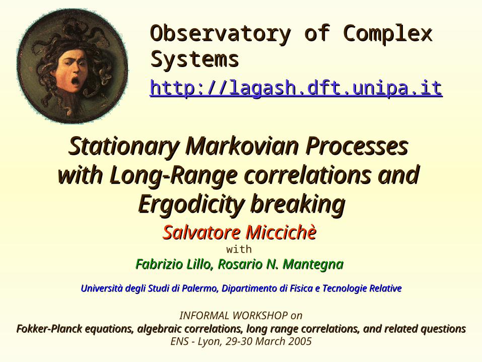
Stationary Markovian Processes Stationary Markovian Processes with Long-Range correlations and with Long-Range correlations and
Ergodicity breakingErgodicity breakingSalvatore MiccichèSalvatore Miccichè
with
Fabrizio Lillo, Rosario N. MantegnaFabrizio Lillo, Rosario N. Mantegna
http://lagash.dft.unipa.ithttp://lagash.dft.unipa.it
Observatory of Complex Observatory of Complex SystemsSystems
Università degli Studi di Palermo, Dipartimento di Fisica e Tecnologie RelativeUniversità degli Studi di Palermo, Dipartimento di Fisica e Tecnologie Relative
INFORMAL WORKSHOP onFokker-Planck equations, algebraic correlations, long range correlations, and related Fokker-Planck equations, algebraic correlations, long range correlations, and related
questionsquestionsENS - Lyon, 29-30 March 2005
Stationary Markovian Processes with Long-Range correlations and Ergodicity Stationary Markovian Processes with Long-Range correlations and Ergodicity breakingbreaking
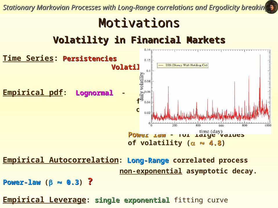
Volatility in Financial MarketsVolatility in Financial Markets
Time Series: PersistenciesPersistencies Volatility ClusteringVolatility Clustering
Empirical pdf: LognormalLognormal - for intermediate values of volatility
Power lawPower law - for large values of volatility ( 4.8 4.8)
Empirical Autocorrelation: Long-RangeLong-Range correlated process
non-exponential asymptotic decay. Power-lawPower-law ( 0.3 0.3) ??
Empirical Leverage: single exponentialsingle exponential fitting curve
MotivationsMotivations
Stationary Markovian Processes with Long-Range correlations and Ergodicity Stationary Markovian Processes with Long-Range correlations and Ergodicity breakingbreaking
MotivationsMotivations
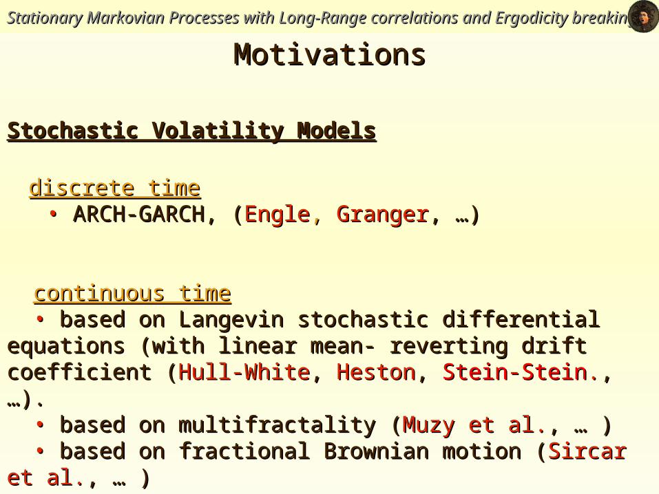
Stochastic Volatility ModelsStochastic Volatility Models
discrete timediscrete time •• ARCH-GARCH, (ARCH-GARCH, (EngleEngle, , GrangerGranger, …), …)
continuous timecontinuous time • • based on Langevin stochastic differential equations (with linear mean- based on Langevin stochastic differential equations (with linear mean- reverting drift coefficient (reverting drift coefficient (Hull-WhiteHull-White, , HestonHeston, , Stein-SteinStein-Stein.., …)., …). •• based on multifractality (based on multifractality (Muzy et al.Muzy et al., … ), … ) •• based on fractional Brownian motion (based on fractional Brownian motion (Sircar et al.Sircar et al., … ), … ) • • ……
Stationary Markovian Processes with Long-Range correlations and Ergodicity Stationary Markovian Processes with Long-Range correlations and Ergodicity breakingbreaking
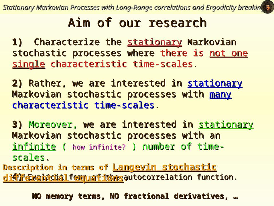
1) 1) Characterize the Characterize the stationarystationary MMarkovian stochastic arkovian stochastic processes whereprocesses where there is there is not one singlenot one single characteristic time-scalescharacteristic time-scales.
2) 2) Rather, we are interested in Rather, we are interested in stationarystationary Markovian Markovian stochastic processes withstochastic processes with manymany characteristic time- characteristic time-scalesscales.
3) 3) Moreover, Moreover, we are interested in we are interested in stationarystationary Markovian Markovian stochastic processes with anstochastic processes with an infiniteinfinite ( ( how infinite?how infinite? ) ) number of time-scalesnumber of time-scales..
4)4) Explicit form of the autocorrelation function.Explicit form of the autocorrelation function.
Aim of our researchAim of our research
Description in terms of Description in terms of Langevin stochastic differential Langevin stochastic differential equationsequations..
NO memory terms, NO fractional derivatives, … NO memory terms, NO fractional derivatives, …
Stationary Markovian Processes with Long-Range correlations and Ergodicity Stationary Markovian Processes with Long-Range correlations and Ergodicity breakingbreaking
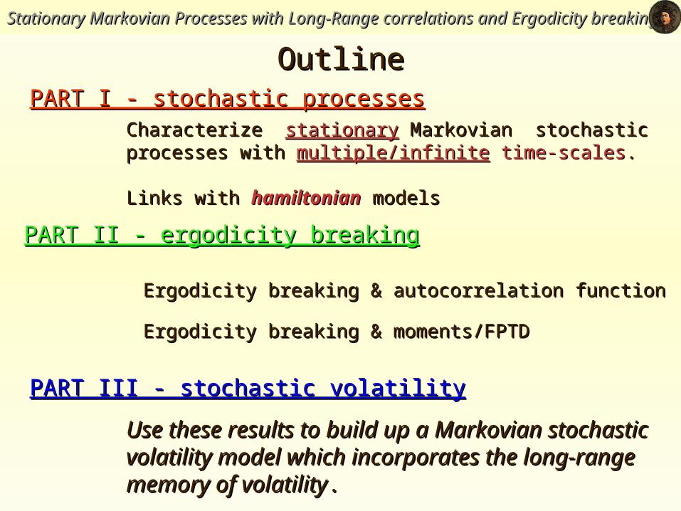
PART I - stochastic processesPART I - stochastic processes
PART III - stochastic volatilityPART III - stochastic volatility
OutlineOutline
CharacterizeCharacterize stationarystationary Markovian stochastic Markovian stochastic processes with processes with multiple/infinitemultiple/infinite time-scales time-scales..
Use these results to build up a Markovian Use these results to build up a Markovian stochastic volatility model which incorporates stochastic volatility model which incorporates the long-range memory of volatilitythe long-range memory of volatility..
PART II - ergodicity breakingPART II - ergodicity breaking
Ergodicity breaking & autocorrelation functionErgodicity breaking & autocorrelation function
Ergodicity breaking & moments/FPTDErgodicity breaking & moments/FPTD
Links with Links with hamiltonianhamiltonian models models
Stationary Markovian Stochastic Processes with Multiple Time-ScalesStationary Markovian Stochastic Processes with Multiple Time-Scales
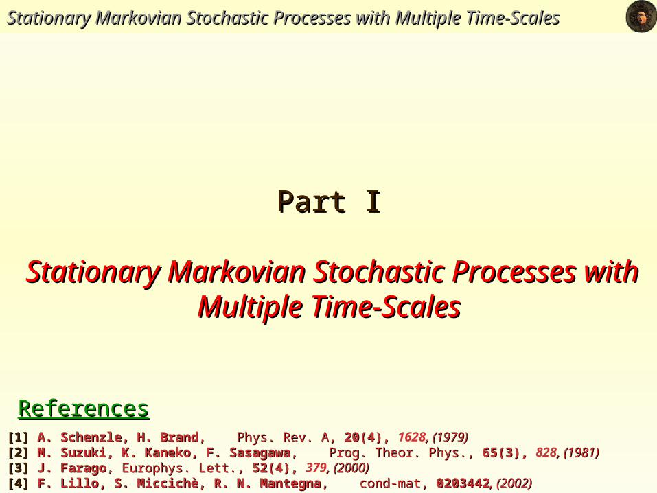
Part IPart I
Stationary Markovian Stochastic Processes Stationary Markovian Stochastic Processes with Multiple Time-Scaleswith Multiple Time-Scales
ReferencesReferences[1] [1] A. Schenzle, H. BrandA. Schenzle, H. Brand, Phys. Rev. A, , Phys. Rev. A, 20(4), 20(4), 1628, (1979) , (1979) [2][2] M. Suzuki, K. Kaneko, F. Sasagawa M. Suzuki, K. Kaneko, F. Sasagawa, Prog. Theor. Phys., , Prog. Theor. Phys., 65(3), 65(3), 828, (1981), (1981)[3][3] J. Farago J. Farago, Europhys. Lett., , Europhys. Lett., 52(4), 52(4), 379, (2000) , (2000) [4][4] F. Lillo, S. Miccichè, R. N. Mantegna F. Lillo, S. Miccichè, R. N. Mantegna, cond-mat, , cond-mat, 02034420203442, (2002), (2002)
Stationary Markovian Stochastic Processes with Multiple Time-ScalesStationary Markovian Stochastic Processes with Multiple Time-Scales
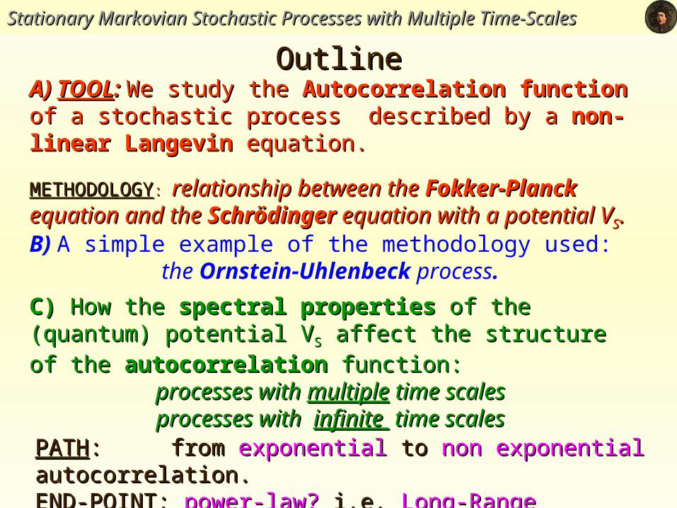
A) A) TOOLTOOL: : We study the We study the Autocorrelation functionAutocorrelation function of of a stochastic process described by a a stochastic process described by a non-linear non-linear LangevinLangevin equation. equation.
METHODOLOGYMETHODOLOGY: : relationship between the relationship between the Fokker-PlanckFokker-Planck equation and the equation and the SchrödingerSchrödinger equation with a equation with a potential Vpotential VSS.. B) A simple example of the methodology used:
the Ornstein-Uhlenbeck process.
C) C) How the How the spectral propertiesspectral properties of the (quantum) potential V of the (quantum) potential VSS
affect the structure of the affect the structure of the autocorrelationautocorrelation function: function:processes with processes with multiplemultiple time scales time scalesprocesses with processes with infinite infinite time scales time scales
OutlineOutline
PATHPATH: : from from exponentialexponential to to non exponential non exponential autocorrelation.autocorrelation.END-POINTEND-POINT:: power-law? power-law? i.e.i.e. Long-Range CorrelatedLong-Range Correlated processes processes ??
Stationary Markovian Stochastic Processes with Multiple Time-ScalesStationary Markovian Stochastic Processes with Multiple Time-Scales
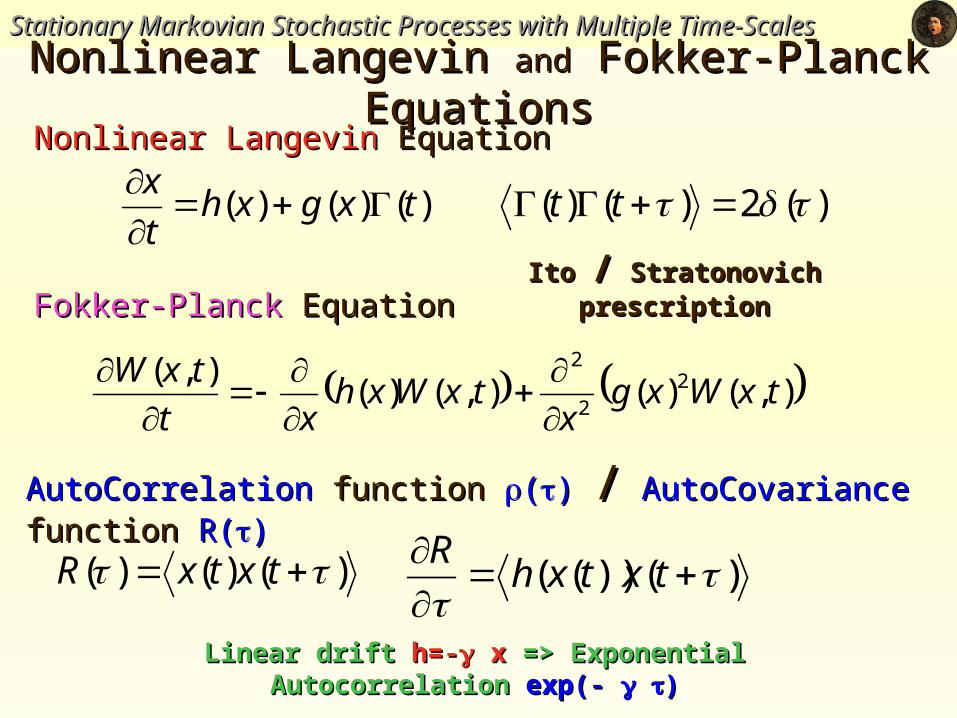
Nonlinear LangevinNonlinear Langevin Equation Equation
Fokker-Planck Fokker-Planck EquationEquation
AutoCorrelationAutoCorrelation function function (()) // AutoCovarianceAutoCovariance function function R(R())
Nonlinear Langevin Nonlinear Langevin andand Fokker-Planck Fokker-Planck EquationsEquations
)()()( txgxht
x
)(2)()( tt
),()(),()(),( 2
2
2
txWxgx
txWxhxt
txW
Linear drift Linear drift h=-h=- x x => Exponential Autocorrelation => Exponential Autocorrelation exp(- exp(- ))
)()()( txtxR )())((
txtxhR
Ito Ito // Stratonovich prescription Stratonovich prescription
Stationary Markovian Stochastic Processes with Multiple Time-ScalesStationary Markovian Stochastic Processes with Multiple Time-Scales
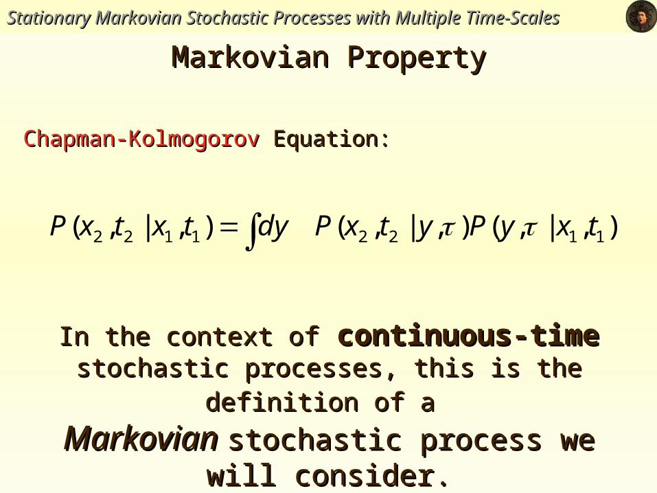
Chapman-Kolmogorov Chapman-Kolmogorov Equation:Equation:
Markovian PropertyMarkovian Property
),|,(),|,(),|,( 11221122 txyPytxPdytxtxP
In the context ofIn the context of continuous-timecontinuous-time stochastic stochastic
processes, this is the definition of aprocesses, this is the definition of a Markovian Markovian stochastic process we will consider.stochastic process we will consider.
Stationary Markovian Stochastic Processes with Multiple Time-ScalesStationary Markovian Stochastic Processes with Multiple Time-Scales
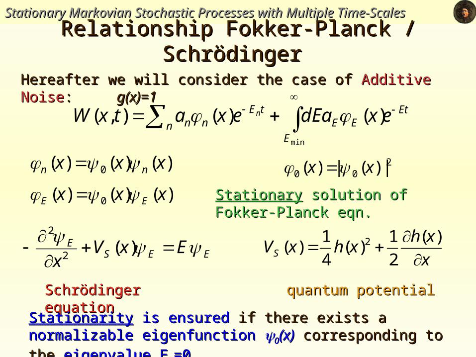
Relationship Fokker-Planck / Schrödinger Relationship Fokker-Planck / Schrödinger
Et
E
EEn
tEnn exdEaexatxW n
min
)()(),(
Hereafter we will consider the case of Hereafter we will consider the case of Additive NoiseAdditive Noise: : g(x)=1g(x)=1
)()()( 0 xxx nn
)()()( 0 xxx EE
EESE ExV
x
)(2
2
x
xhxhxVS
)(
2
1)(
4
1)( 2
200 |)(|)( xx
StationaryStationary solution of Fokker-Planck eqn. solution of Fokker-Planck eqn.
Schrödinger equationSchrödinger equation quantum potentialquantum potential
StationarityStationarity is ensured is ensured if there exists aif there exists a normalizable eigenfunction normalizable eigenfunction 00(x)(x)
corresponding to thecorresponding to the eigenvalue E eigenvalue E00=0.=0.
Stationary Markovian Stochastic Processes with Multiple Time-ScalesStationary Markovian Stochastic Processes with Multiple Time-Scales
Relationship Fokker-Planck / Schrödinger Relationship Fokker-Planck / Schrödinger
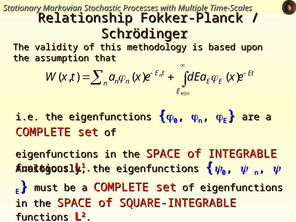
The validity of this methodology is based upon the assumption thatThe validity of this methodology is based upon the assumption that
i.e. the eigenfunctions i.e. the eigenfunctions {{00, , nn, , EE}} are a are a COMPLETECOMPLETE setset of of
eigenfunctions in the eigenfunctions in the SPACE of INTEGRABLESPACE of INTEGRABLE functions functions LL11..
Analogously, the eigenfunctions Analogously, the eigenfunctions {{00, , nn, , EE}} must be a must be a
COMPLETECOMPLETE setset of eigenfunctions in the of eigenfunctions in the SPACE of SPACE of SQUARE-INTEGRABLESQUARE-INTEGRABLE functions functions LL22..
Et
E
EEn
tEnn exdEaexatxW n
min
)()(),(
Stationary Markovian Stochastic Processes with Multiple Time-ScalesStationary Markovian Stochastic Processes with Multiple Time-Scales
Relationship Fokker-Planck / Schrödinger Relationship Fokker-Planck / Schrödinger
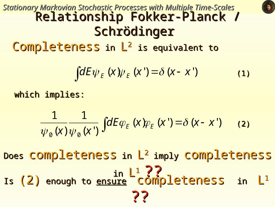
CompletenessCompleteness in in LL22 is equivalent to is equivalent to
)'()'()( xxxxdE EE
Is Is (2)(2) enough to enough to ensureensure completeness completeness in in LL11 ????
)'()'()()'(
1
)(
1
00
xxxxdExx EE
Does Does completenesscompleteness in in LL22 imply imply completenesscompleteness in in LL1 1 ????
(1)(1)
(2)(2)
which implies: which implies:
Stationary Markovian Stochastic Processes with Multiple Time-ScalesStationary Markovian Stochastic Processes with Multiple Time-Scales
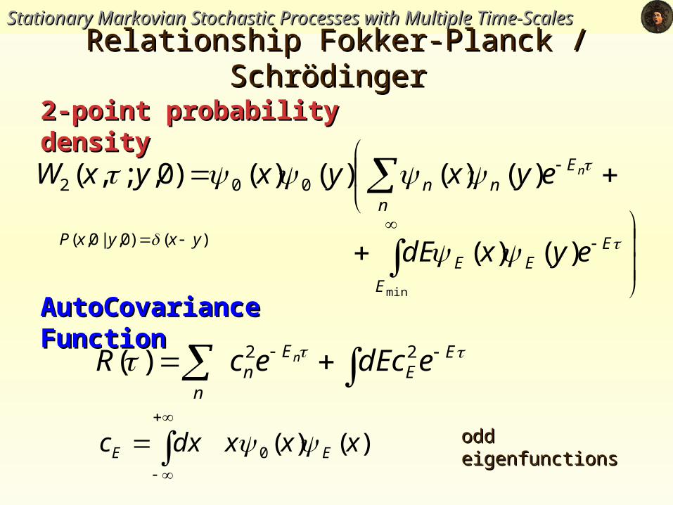
AutoCovariance FunctionAutoCovariance Function
Relationship Fokker-Planck / Schrödinger Relationship Fokker-Planck / Schrödinger
nE
nn
n eyxyxyxW )()()()()0,;,( 002
2-point probability density2-point probability density
)()(0 xxxdxc EE
EE
En
n
ecdEecR n 22)(
EEE
E
eyxdE )()(min
odd eigenfunctionsodd eigenfunctions
)()0,|0,( yxyxP
Stationary Markovian Stochastic Processes with Multiple Time-ScalesStationary Markovian Stochastic Processes with Multiple Time-Scales
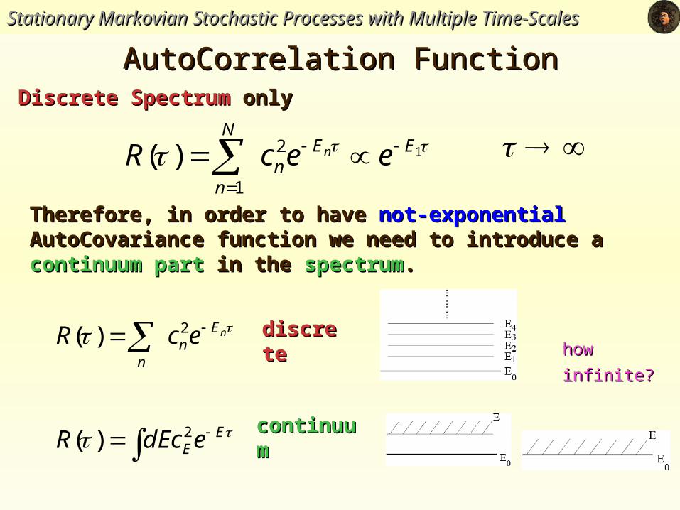
AutoCorrelation FunctionAutoCorrelation FunctionDiscrete SpectrumDiscrete Spectrum only only
Therefore, in order to have Therefore, in order to have not-exponentialnot-exponential AutoCovariance function AutoCovariance function we need to introduce a we need to introduce a continuum partcontinuum part in the in the spectrumspectrum..
12
1
)( EEn
N
n
eecR n
nEn
n
ecR 2)(
EEecdER 2)(
discretediscrete
continuumcontinuum
how how
infinite?infinite?
Stationary Markovian Stochastic Processes with Multiple Time-ScalesStationary Markovian Stochastic Processes with Multiple Time-Scales
Ornstein-Uhlenbeck processOrnstein-Uhlenbeck process
Linear driftLinear drift
Exponential autocorrelation expectedExponential autocorrelation expected
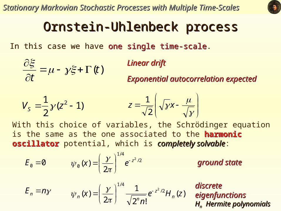
In this case we have one single time-scale.
)(tt
)1(2
1 2 zVS
xz
2
1
In this case we have one single time-scaleone single time-scale.
With this choice of variables, the Schrödinger equation is the same as the one associated to the harmonic oscillatorharmonic oscillator potential, which is completely solvablecompletely solvable:
2/4/1
0
2
2)( zex
)(!2
1
2)( 2/
4/12
zHen
x nz
nn
00 E
nEn
ground stateground state
discrete eigenfunctionsdiscrete eigenfunctionsHHnn Hermite polynomials Hermite polynomials
Stationary Markovian Stochastic Processes with Multiple Time-ScalesStationary Markovian Stochastic Processes with Multiple Time-Scales
Ornstein-Uhlenbeck processOrnstein-Uhlenbeck process
01
11
n
ncn
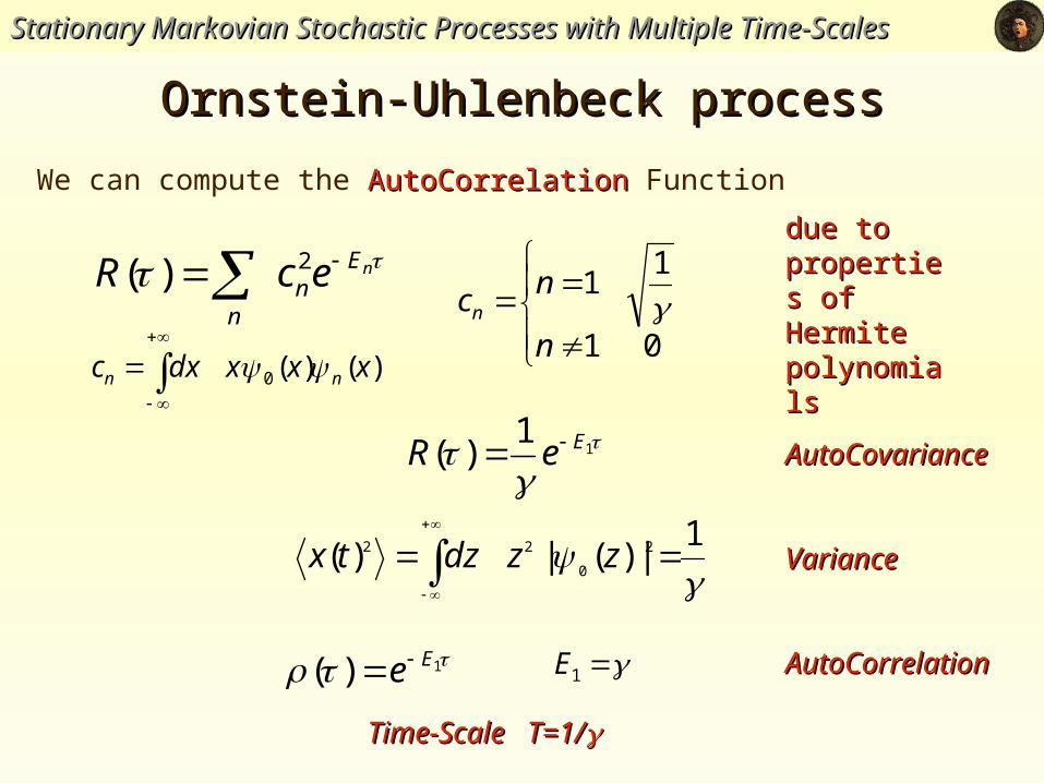
We can compute the AutoCorrelationAutoCorrelation Function
AutoCovarianceAutoCovariance
nEn
n
ecR 2)(
1
1)( EeR
due to due to properties of properties of Hermite Hermite polynomialspolynomials
1
|)(|)( 2
0
22
zzdztx VarianceVariance
1)( Ee AutoCorrelationAutoCorrelation
)()(0 xxxdxc nn
1E
Time-Scale T=1/Time-Scale T=1/
Stationary Markovian Stochastic Processes with Multiple Time-ScalesStationary Markovian Stochastic Processes with Multiple Time-Scales
The Square Well The Square Well
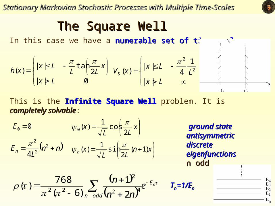
0||
2tan||
)(Lx
xLL
Lxxh
In this case we have a numerable set of time-scalesnumerable set of time-scales.
Lx
LLx
xVS
||
1
4||
)( 2
2
x
LLx
2cos
1)(0
xn
LLxn )1(
2sin
1)(
00 E
nnL
En 22
2
4
ground stateground state
antisymmetricantisymmetricdiscrete eigenfunctionsdiscrete eigenfunctionsn oddn odd
nE
oddn
enn
n
42
2
222
1
)6(
768)(
This is the Infinite Square Well Infinite Square Well problem. It is completely solvablecompletely solvable:
TTnn=1/E=1/Enn
Stationary Markovian Stochastic Processes with Multiple Time-ScalesStationary Markovian Stochastic Processes with Multiple Time-Scales
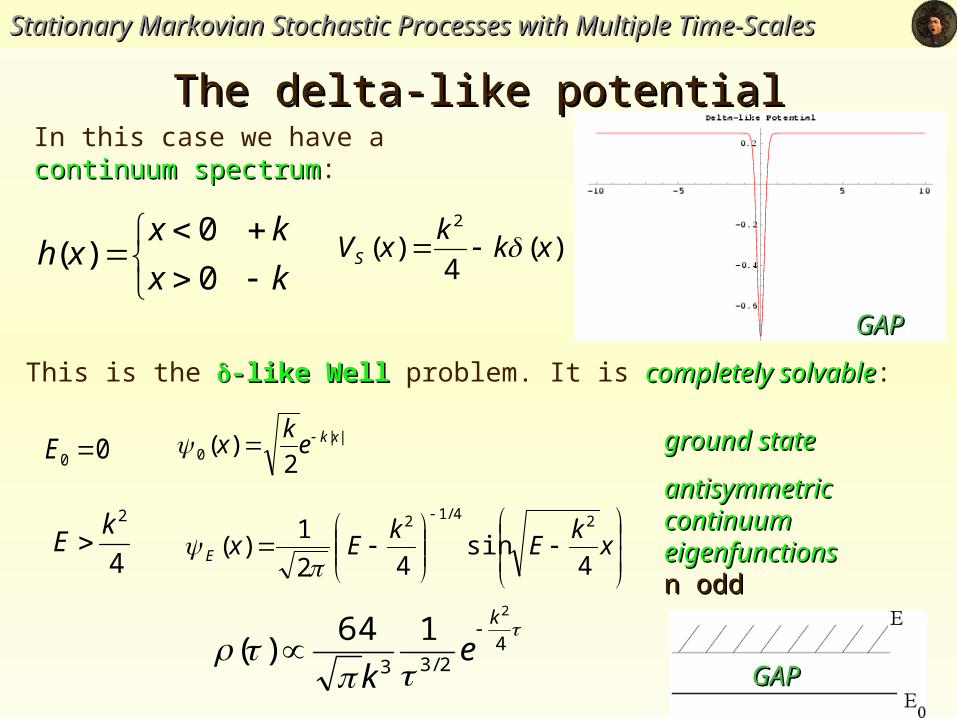
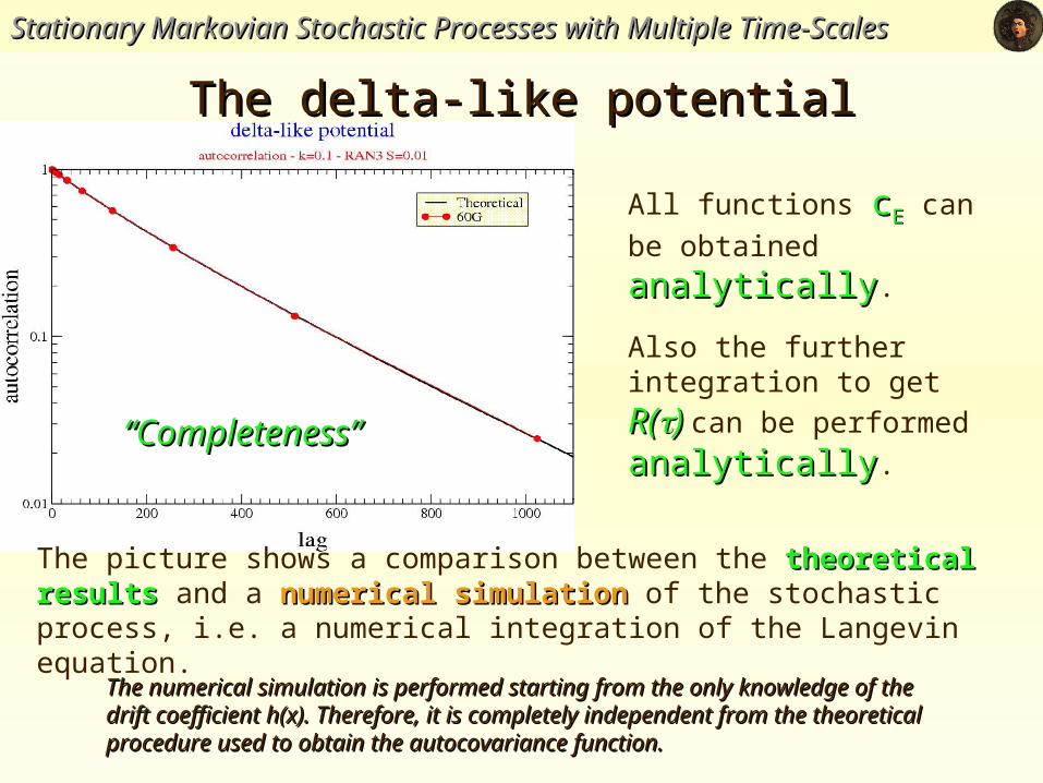
The delta-like potentialThe delta-like potentialIn this case we have a continuum spectrumcontinuum spectrum:
kx
kxxh
0
0)( )(
4)(
2
xkk
xVS
||0 2
)( xkek
x
xk
Ek
ExE 4sin
42
1)(
24/12
00 E
4
2kE
ground stateground state
antisymmetricantisymmetriccontinuum eigenfunctionscontinuum eigenfunctionsn oddn odd
4
2/33
2
164)(
k
ek
This is the -like Well-like Well problem. It is completely solvablecompletely solvable:
GAPGAP
GAPGAP
Stationary Markovian Stochastic Processes with Multiple Time-ScalesStationary Markovian Stochastic Processes with Multiple Time-Scales
The delta-like potentialThe delta-like potential
All functions ccEE can be
obtained analyticallyanalytically.
Also the further integration to
get R(R()) can be performed
analyticallyanalytically.
The picture shows a comparison between the theoretical resultstheoretical results and a numerical numerical simulationsimulation of the stochastic process, i.e. a numerical integration of the Langevin equation.
The numerical simulation is performed starting from the only knowledge of the drift The numerical simulation is performed starting from the only knowledge of the drift coefficient h(x). Therefore, it is completely independent from the theoretical procedure coefficient h(x). Therefore, it is completely independent from the theoretical procedure used to obtain the autocovariance function.used to obtain the autocovariance function.
““Completeness”Completeness”
Stationary Markovian Stochastic Processes with Multiple Time-ScalesStationary Markovian Stochastic Processes with Multiple Time-Scales
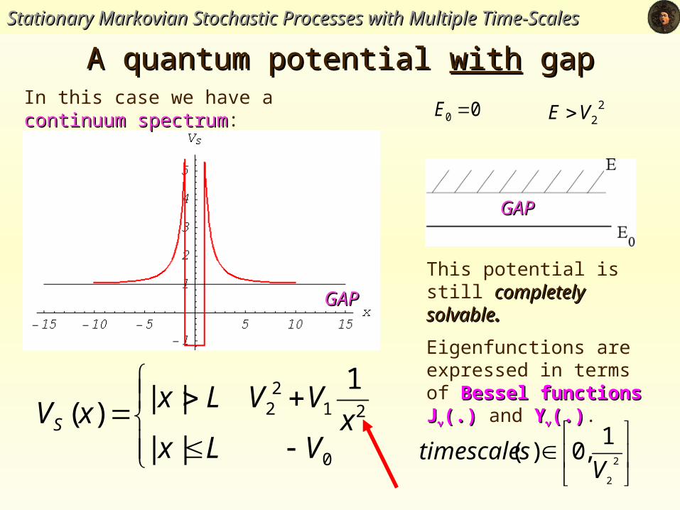
A quantum potential A quantum potential withwith gap gap
0
212
2
||
1||)(
VLxx
VVLxxVS
In this case we have a continuum spectrumcontinuum spectrum:
This potential is still completely solvablecompletely solvable..
Eigenfunctions are expressed in terms of Bessel functions Bessel functions JJ(.)(.) and YY(.)(.).
GAPGAP
GAPGAP
00 E
2
2
1,0)(V
stimescale
22VE
Stationary Markovian Stochastic Processes with Multiple Time-ScalesStationary Markovian Stochastic Processes with Multiple Time-Scales
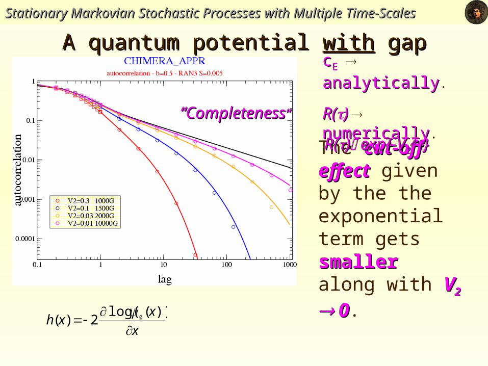
A quantum potential A quantum potential withwith gap gap
ccEE analyticallyanalytically.
R(R()) numericallynumerically.
The cut-off effectcut-off effect given by the the exponential term gets smallersmaller along with VV2 2 0 0.
R(R()) exp{-V exp{-V2222}}
““CompletenessCompleteness““
x
xxh
))(log(
2)( 0
So far: continuum spectrumcontinuum spectrum non exponentialnon exponential autocorrelation
Stationary Markovian Stochastic Processes with Multiple Time-ScalesStationary Markovian Stochastic Processes with Multiple Time-Scales
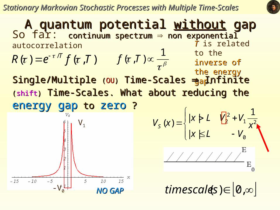
A quantum potential A quantum potential withoutwithout gap gap
1
),( TfTT is related to the inverse of the inverse of the energy gapenergy gap..
),()( / TfeR T
Single/MultipleSingle/Multiple ((OUOU)) Time-ScalesTime-Scales InfiniteInfinite ((shiftshift)) Time-Scales. What Time-Scales. What
about reducing theabout reducing the energy gapenergy gap to to zerozero ? ?
0
212
2
||
1||)(
VLxx
VVLxxVS
NO GAPNO GAP
V1
-V0 ,0)(stimescale
Eigenfunctions x>L
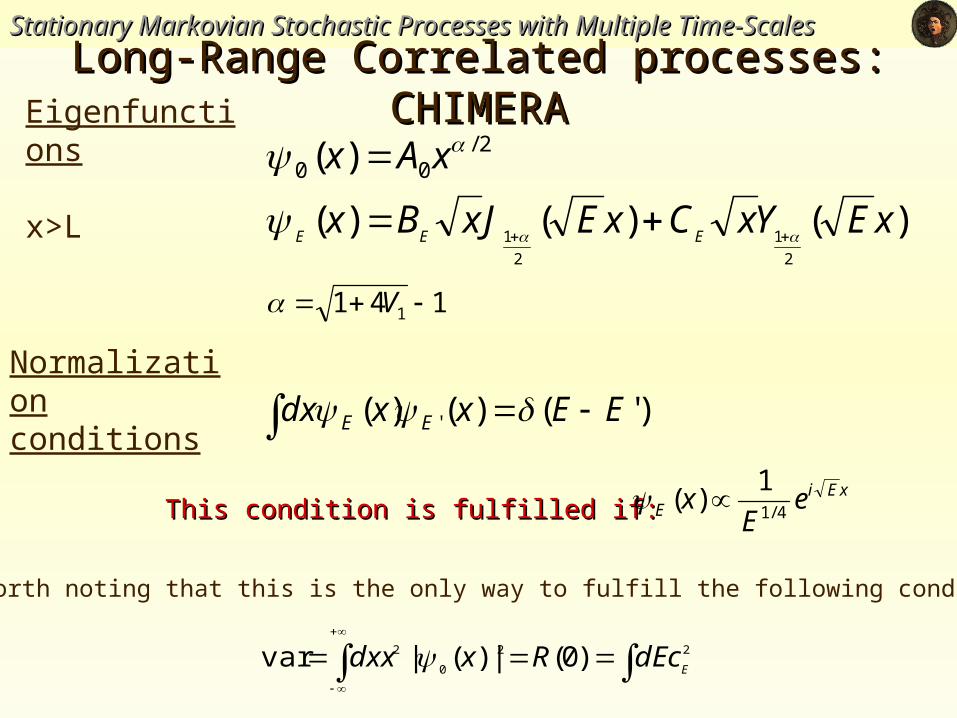
Stationary Markovian Stochastic Processes with Multiple Time-ScalesStationary Markovian Stochastic Processes with Multiple Time-ScalesLong-Range Correlated processes: Long-Range Correlated processes:
CHIMERACHIMERA2/
00 )( xAx
)()()(2
1
2
1xEYxCxEJxBx
EEE
)'()()( ' EExxdx EE
This condition is fulfilled if:This condition is fulfilled if:xEi
E eE
x4/1
1)(
It is worth noting that this is the only way to fulfill the following condition:
22
0
2 )0(|)(|varE
cdERxdxx
Normalizationconditions
141 1 V
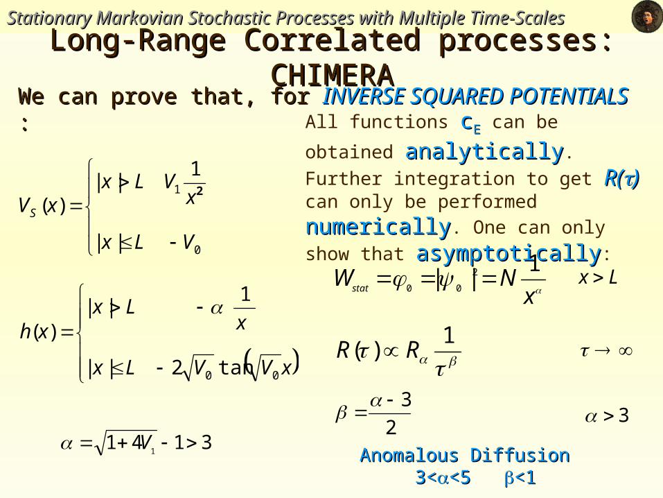
Stationary Markovian Stochastic Processes with Multiple Time-ScalesStationary Markovian Stochastic Processes with Multiple Time-ScalesLong-Range Correlated processes: Long-Range Correlated processes:
CHIMERACHIMERA
0
1
||
1||
)(
VLx
xVLx
xVS
2
We can prove that, for We can prove that, for INVERSE SQUARED POTENTIALS INVERSE SQUARED POTENTIALS ::
xVVLx
xLx
xh
00 tan2||
1||
)(
All functions ccEE can be obtained
analyticallyanalytically. Further integration to get
R(R()) can only be performed numericallynumerically.
One can only show that asymptoticallyasymptotically:
31411
V
1
)( RR
2
3
xNW
stat
1|| 2
00
3
Lx
Anomalous Diffusion 3<Anomalous Diffusion 3<<5 <5 <1<1
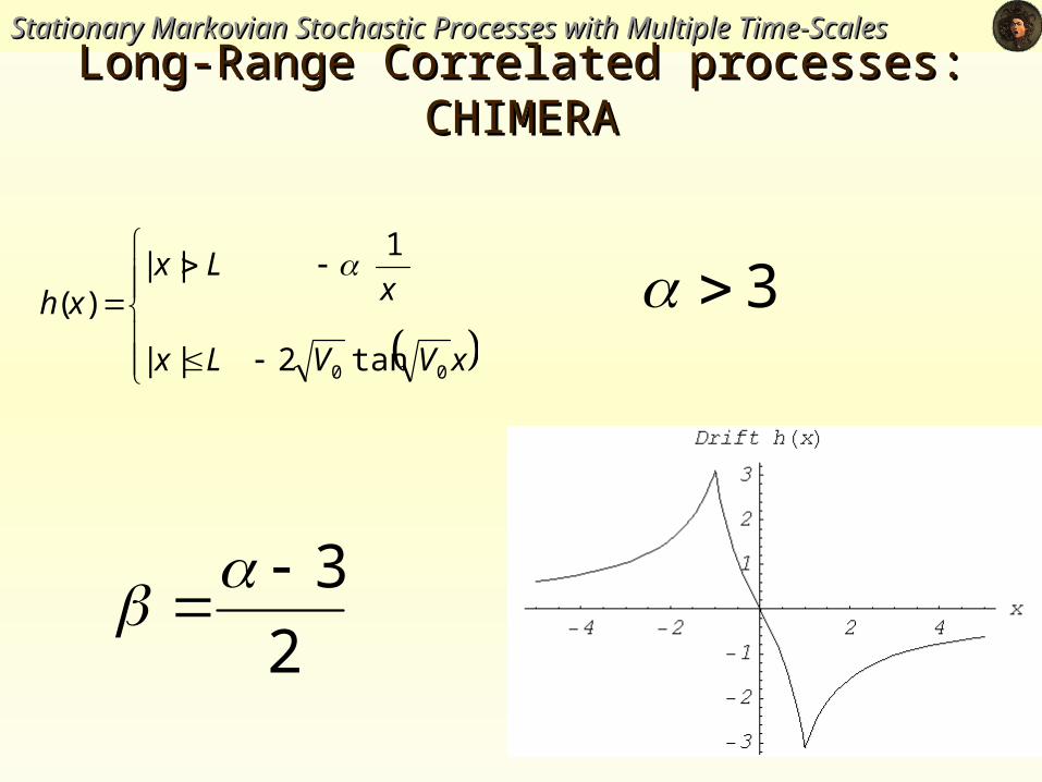
Stationary Markovian Stochastic Processes with Multiple Time-ScalesStationary Markovian Stochastic Processes with Multiple Time-ScalesLong-Range Correlated processes: Long-Range Correlated processes:
CHIMERACHIMERA
xVVLx
xLx
xh
00 tan2||
1||
)( 3
2
3
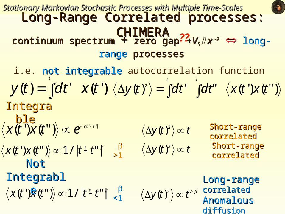
continuum spectrum continuum spectrum ++ zero gap zero gap ++VVS S x x -2-2 long-rangelong-range processes processes
i.e. not integrablenot integrable autocorrelation function
Stationary Markovian Stochastic Processes with Multiple Time-ScalesStationary Markovian Stochastic Processes with Multiple Time-ScalesLong-Range Correlated processes: Long-Range Correlated processes:
CHIMERACHIMERA
t
txdtty )'(')( t t
txtxdtdtty )"()'("')( 2
|"'|)"()'( ttetxtx
|"'|/1)"()'( tttxtx
|"'|/1)"()'( tttxtx
tty 2)(
tty 2)(
22)( tty
>1>1
<1<1
Short-range correlatedShort-range correlated
Short-range correlatedShort-range correlated
Long-rangeLong-range correlated correlated
AnomalousAnomalous diffusion diffusion
??
Not IntegrableNot Integrable
Integrable Integrable
Stationary Markovian Stochastic Processes with Multiple Time-ScalesStationary Markovian Stochastic Processes with Multiple Time-ScalesLong-Range Correlated processes: Long-Range Correlated processes:
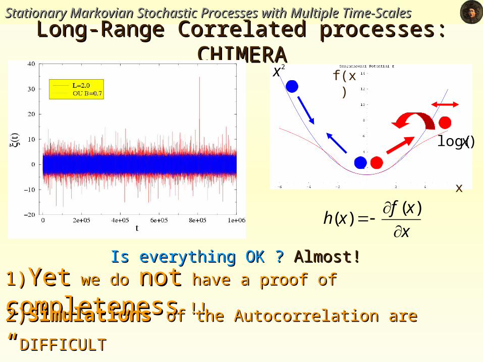
CHIMERACHIMERA
x
xfxh
)(
)(
Is everything OK ? Is everything OK ? Almost!Almost!
1)1)YetYet we do we do notnot have a proof of have a proof of
completenesscompleteness !! !!
2)2)SimulationsSimulations of the Autocorrelation areof the Autocorrelation are “ “DIFFICULTDIFFICULT””
x
f(x)
)log(x
2x
Stationary Markovian Stochastic Processes with Multiple Time-ScalesStationary Markovian Stochastic Processes with Multiple Time-ScalesLong-Range Correlated processes: Long-Range Correlated processes:
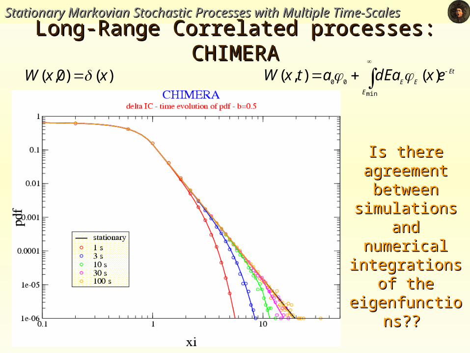
CHIMERACHIMERA
Is there Is there agreement agreement between between
simulations simulations and numerical and numerical integrations of integrations of
the the eigenfunctionseigenfunctions
????
Et
E
EEexdEaatxW
min
00)(),( )()0,( xxW
Stationary Markovian Stochastic Processes with Multiple Time-ScalesStationary Markovian Stochastic Processes with Multiple Time-ScalesLong-Range Correlated processes: Long-Range Correlated processes:
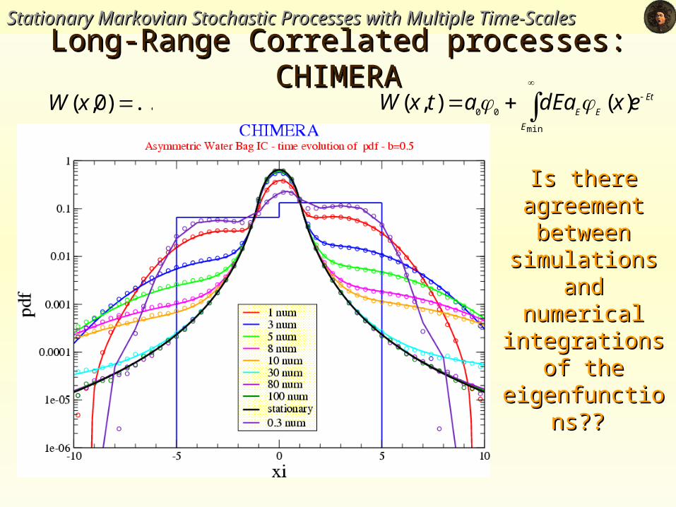
CHIMERACHIMERA
Is there Is there agreement agreement between between
simulations simulations and numerical and numerical integrations of integrations of
the the eigenfunctionseigenfunctions
????
Et
E
EEexdEaatxW
min
00)(),( ...)0,( xW
Stationary Markovian Stochastic Processes with Multiple Time-ScalesStationary Markovian Stochastic Processes with Multiple Time-Scales
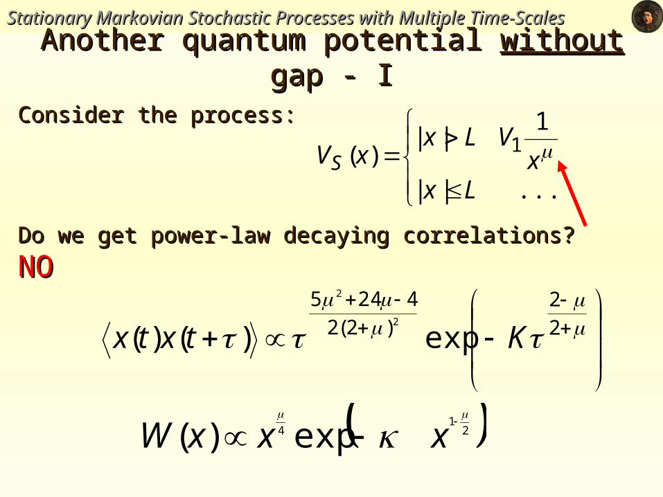
Another quantum potential Another quantum potential withoutwithout gap - I gap - I
Consider the process:Consider the process:
....||
1||
)( 1
Lxx
VLxxVS
Do we get power-law decaying correlations? Do we get power-law decaying correlations? NONO
2
2)2(2
4245
exp)()(2
2
Ktxtx
21
4 exp)(
xxxW
Stationary Markovian Stochastic Processes with Multiple Time-ScalesStationary Markovian Stochastic Processes with Multiple Time-Scales
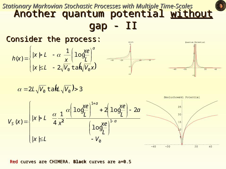
Another quantum potential Another quantum potential withoutwithout gap - II gap - II
Consider the process:Consider the process:
xVVLxL
xe
xLx
xh
a
00 tan2||
log1
||)(
3tan2 00 VLVL
0
1
1
||
log
2log2log1
4||
)(
VLxLxe
aLxe
Lxe
xLx
xV a
a
S
2
RedRed curves are CHIMERA. curves are CHIMERA. BlackBlack curves are a=0.5 curves are a=0.5
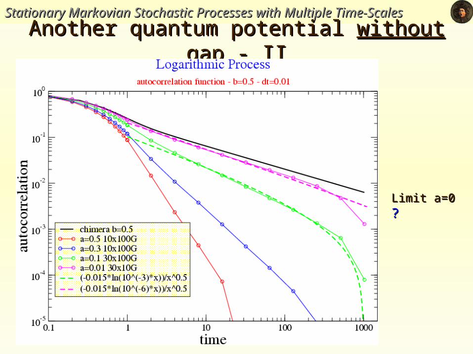
Stationary Markovian Stochastic Processes with Multiple Time-ScalesStationary Markovian Stochastic Processes with Multiple Time-Scales
Another quantum potential Another quantum potential withoutwithout gap - II gap - II
Limit a=0Limit a=0 ? ?
Stationary Markovian Stochastic Processes with Multiple Time-ScalesStationary Markovian Stochastic Processes with Multiple Time-Scales
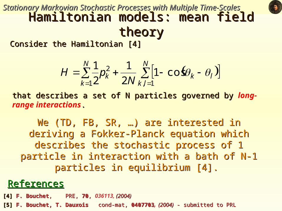
Hamiltonian models: mean field theoryHamiltonian models: mean field theory
We (TD, FB, SR, …) are interested in deriving a We (TD, FB, SR, …) are interested in deriving a Fokker-Planck equation which describes the Fokker-Planck equation which describes the
stochastic process of 1 particle in interaction with a stochastic process of 1 particle in interaction with a bath of N-1 particles in equilibrium [4].bath of N-1 particles in equilibrium [4].
Consider the Hamiltonian [4]Consider the Hamiltonian [4]
that describes a set of N particles governed by that describes a set of N particles governed by long-range interactions..
ReferencesReferences[4][4] F. Bouchet F. Bouchet, PRE, , PRE, 7070, , 036113, (2004)(2004)
[5][5] F. Bouchet, T. Dauxois F. Bouchet, T. Dauxois cond-mat, cond-mat, 04077030407703, (2004)(2004) - submitted to PRL - submitted to PRL
N
lklkk
N
k NpH
1,
2
1cos1
2
1
2
1
Stationary Markovian Stochastic Processes with Multiple Time-ScalesStationary Markovian Stochastic Processes with Multiple Time-Scales
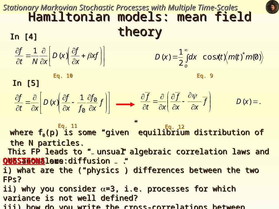
Hamiltonian models: mean field theoryHamiltonian models: mean field theoryIn [4]In [4]
In [5]In [5]Eq. 10Eq. 10
This FP leads to “This FP leads to “… … unsual algebraic correlation laws and to anomalous diffusion unsual algebraic correlation laws and to anomalous diffusion ……”.”.
where fwhere f00(p) is some “given” equilibrium distribution of the N particles.(p) is some “given” equilibrium distribution of the N particles.
QUESTIONSQUESTIONS are: are:i) what are the (“physics”) differences between the two FPs?i) what are the (“physics”) differences between the two FPs?ii) why you consider ii) why you consider =3, i.e. processes for which variance is not well defined?=3, i.e. processes for which variance is not well defined?iii) how do you write the cross-correlations between particles ?iii) how do you write the cross-correlations between particles ?
xfx
fxD
xNt
f )(1
Eq. 11Eq. 11 Eq. 12Eq. 12
Eq. 9Eq. 9
)0()()cos(2
1)( *mtmxtdxxD
o
fx
f
fx
fxD
xt
f 0
0
1)(
fxx
f
xt
f ...)( xD
ConclusionsConclusionsStationary Markovian Stochastic Processes with Multiple Time-ScalesStationary Markovian Stochastic Processes with Multiple Time-Scales
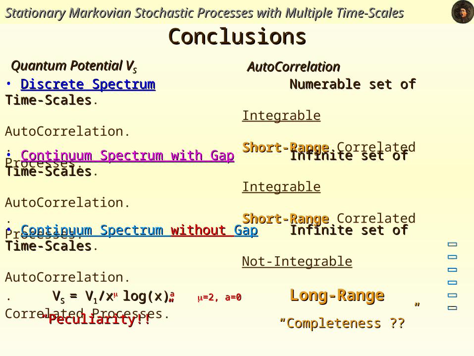
• Discrete SpectrumDiscrete Spectrum Numerable set of Time-ScalesNumerable set of Time-Scales. Integrable AutoCorrelation.. Short-RangeShort-Range Correlated Processes.
• Continuum Spectrum with GapContinuum Spectrum with Gap Infinite set of Time-ScalesInfinite set of Time-Scales. Integrable AutoCorrelation.. Short-RangeShort-Range Correlated Processes.
• Continuum Spectrum Continuum Spectrum without without GapGap Infinite set of Time-ScalesInfinite set of Time-Scales. Not-Integrable AutoCorrelation.
. VVS S = V= V11/x/x log(x)log(x)aa =2, a=0=2, a=0 Long-RangeLong-Range Correlated Processes.
““Completeness ??”Completeness ??”
Quantum Potential VQuantum Potential VSS AutoCorrelationAutoCorrelation
““Peculiarity!! ”Peculiarity!! ”
Ergodicity breakingErgodicity breaking
Part IIPart II
Ergodicity BreakingErgodicity Breaking
ReferencesReferences[1] [1] E. LutzE. Lutz, PRL, , PRL, 9393, , 190602, , (2004)(2004)[2][2] S. Miccichè, F. Lillo, R. N. Mantegna S. Miccichè, F. Lillo, R. N. Mantegna, in preparation, in preparation[3] [3] J.-P. BouchaudJ.-P. Bouchaud, J. Phys. I France, , J. Phys. I France, 22, , 1705, , (1992)(1992)[4][4] G. Bel, E. Barkai G. Bel, E. Barkai, cond-mat/0502154, cond-mat/0502154
Ergodicity breakingErgodicity breaking
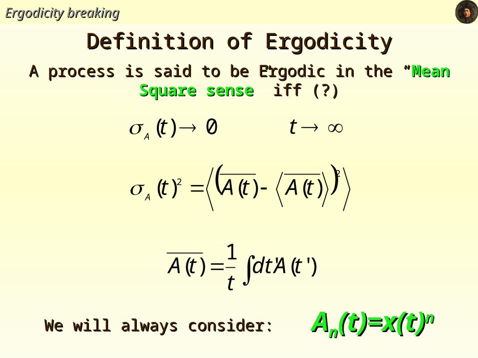
A process is said to be Ergodic in the “A process is said to be Ergodic in the “Mean Square Mean Square sensesense” iff (?)” iff (?)
22 )()()( tAtAtA
0)( tA
t
)'('1
)( tAdtt
tA
Definition of ErgodicityDefinition of Ergodicity
We will always consider: We will always consider: AAnn(t)=x(t)(t)=x(t)nn
Ergodicity breakingErgodicity breaking
Ergodicity for CHIMERAErgodicity for CHIMERA
ttA
2)(
2
)12(
n
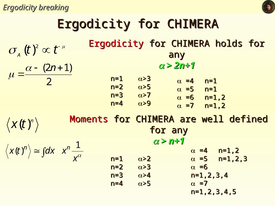
ErgodicityErgodicity for CHIMERA holds for any for CHIMERA holds for any > 2n+1 > 2n+1
n=1n=1 >3>3n=2n=2 >5>5n=3n=3 >7>7n=4n=4 >9>9
ntx )( MomentsMoments for CHIMERA are well defined for for CHIMERA are well defined for anyany
> n+1 > n+1
n=1n=1 >2>2n=2n=2 >3>3n=3n=3 >4>4n=4n=4 >5>5
=4=4 n=1,2n=1,2 =5 =5 n=1,2,3n=1,2,3 =6 =6 n=1,2,3,4n=1,2,3,4 =7 =7n=1,2,3,4,5n=1,2,3,4,5
=4=4 n=1n=1 =5 =5 n=1n=1 =6 =6 n=1,2n=1,2 =7 =7 n=1,2n=1,2
xxdxtx nn 1
)(
Ergodicity breakingErgodicity breaking
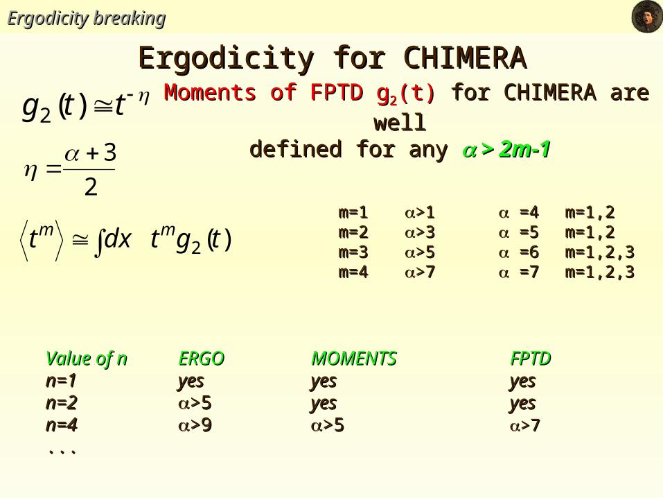
ttg )(2 Moments of FPTD gMoments of FPTD g22(t)(t) for CHIMERA are well for CHIMERA are well defined for any defined for any > 2m-1 > 2m-1
=4=4 m=1,2m=1,2 =5 =5 m=1,2m=1,2 =6 =6m=1,2,3m=1,2,3 =7 =7m=1,2,3m=1,2,3
Value of nValue of n ERGOERGO MOMENTSMOMENTS FPTDFPTDn=1n=1 yesyes yesyes yesyesn=2n=2 >5>5 yes yes yesyes n=4n=4 >9>9 >5>5 >7>7 ......
Ergodicity for CHIMERAErgodicity for CHIMERA
m=1m=1 >1>1m=2m=2 >3>3m=3m=3 >5>5m=4m=4 >7>7
)(2 tgtdxt mm
2
3
Ergodicity breakingErgodicity breaking
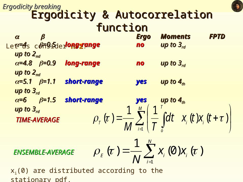
Let us consider n=2n=2:
Ergodicity & Autocorrelation functionErgodicity & Autocorrelation function
ErgoErgo MomentsMoments FPTDFPTD=4=4 =0.5=0.5 long-rangelong-range nono up to 3up to 3rd rd up to 2up to 2ndnd
=4.8=4.8 =0.9=0.9 long-rangelong-range nono up to 3up to 3rd rd up to 2up to 2ndnd
=5.1=5.1 =1.1=1.1 short-rangeshort-range yesyes up to 4up to 4thth up to up to 33rdrd
=6=6 =1.5=1.5 short-rangeshort-range yesyes up to 4up to 4th th up to 3up to 3rdrd
TIME-AVERAGETIME-AVERAGE
ENSEMBLE-ENSEMBLE-AVERAGEAVERAGE
N
iiiE
xxN 1
)()0(1
)(
M
i
T
o
iiTtxtxdt
TM 1
)()(11
)(
xi(0) are distributed according to the stationary pdf.
Ergodicity breakingErgodicity breaking
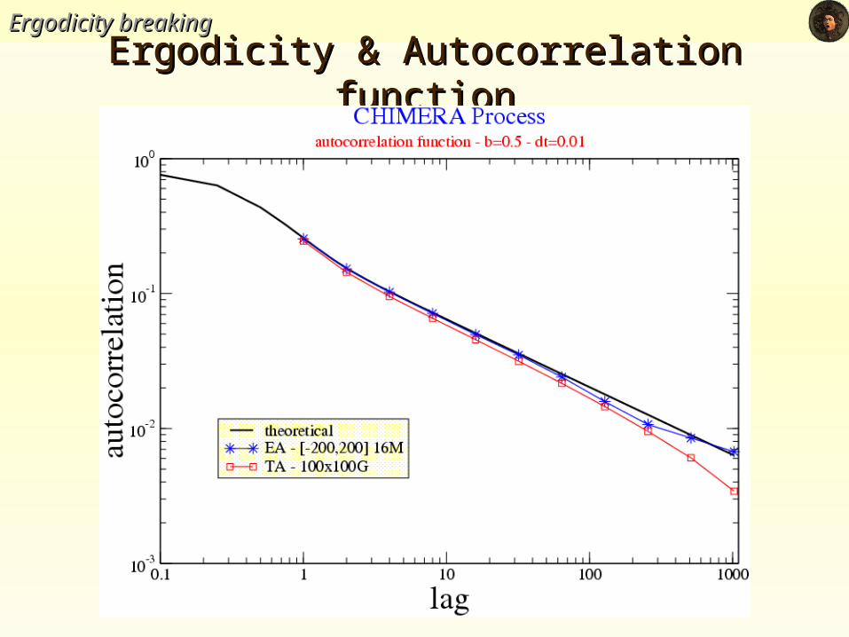
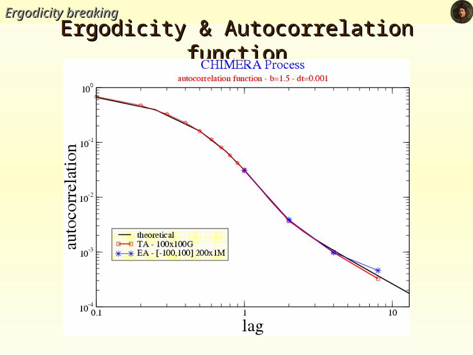
Ergodicity & Autocorrelation functionErgodicity & Autocorrelation function
Ergodicity breakingErgodicity breaking
Ergodicity & Autocorrelation functionErgodicity & Autocorrelation function
Ergodicity breakingErgodicity breaking
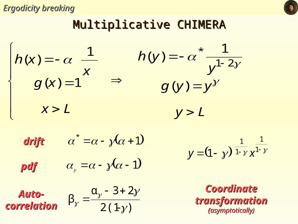
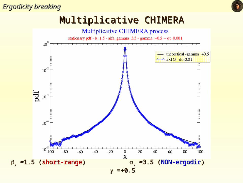
Multiplicative CHIMERAMultiplicative CHIMERA
)-2(1
23αβ
Ly
yyg
yyh
Lx
xgx
xh
)(
1)(
1)(
1)( 21
*
1 pdfpdf
Auto-Auto-correlatiocorrelatio
nn
driftdrift 1*
CoordinateCoordinatetransformationtransformation
((asymptotically)asymptotically)
1
1
1
1
1 xy
Ergodicity breakingErgodicity breaking
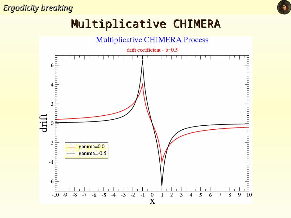
Multiplicative CHIMERAMultiplicative CHIMERA
Ergodicity breakingErgodicity breaking
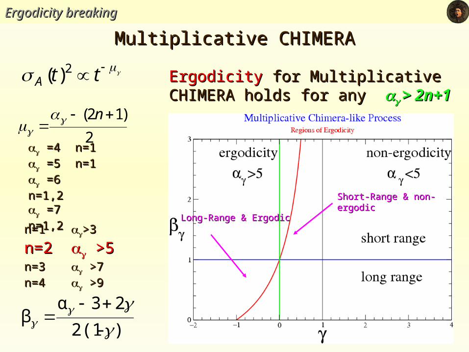
Multiplicative CHIMERAMultiplicative CHIMERA
ttA2)(
2
)12(
n
ErgodicityErgodicity for Multiplicative CHIMERA for Multiplicative CHIMERA holds for any holds for any > 2n+1> 2n+1
n=1n=1 >3>3
n=2n=2 >5 >5n=3n=3 >7 >7n=4n=4 >9 >9
=4=4 n=1n=1 =5 =5 n=1n=1 =6 =6n=1,2n=1,2 =7 =7n=1,2n=1,2
)-2(1
23αβ
Short-Range & non-Short-Range & non-ergodicergodic
Long-Range & ErgodicLong-Range & Ergodic
Ergodicity breakingErgodicity breaking
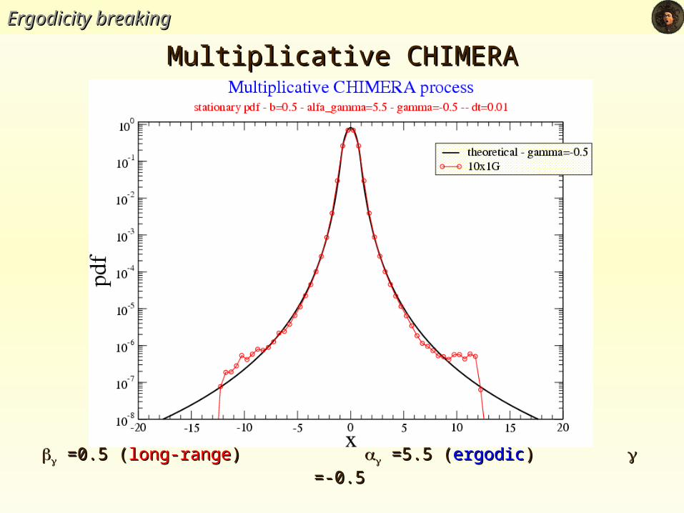
Multiplicative CHIMERAMultiplicative CHIMERA
=0.5 (=0.5 (long-rangelong-range) ) =5.5 ( =5.5 (ergodicergodic) ) =-0.5 =-0.5
Ergodicity breakingErgodicity breaking
Multiplicative CHIMERAMultiplicative CHIMERA
=1.5 (=1.5 (short-rangeshort-range) ) =3.5 ( =3.5 (NON-ergodicNON-ergodic) ) =+0.5 =+0.5
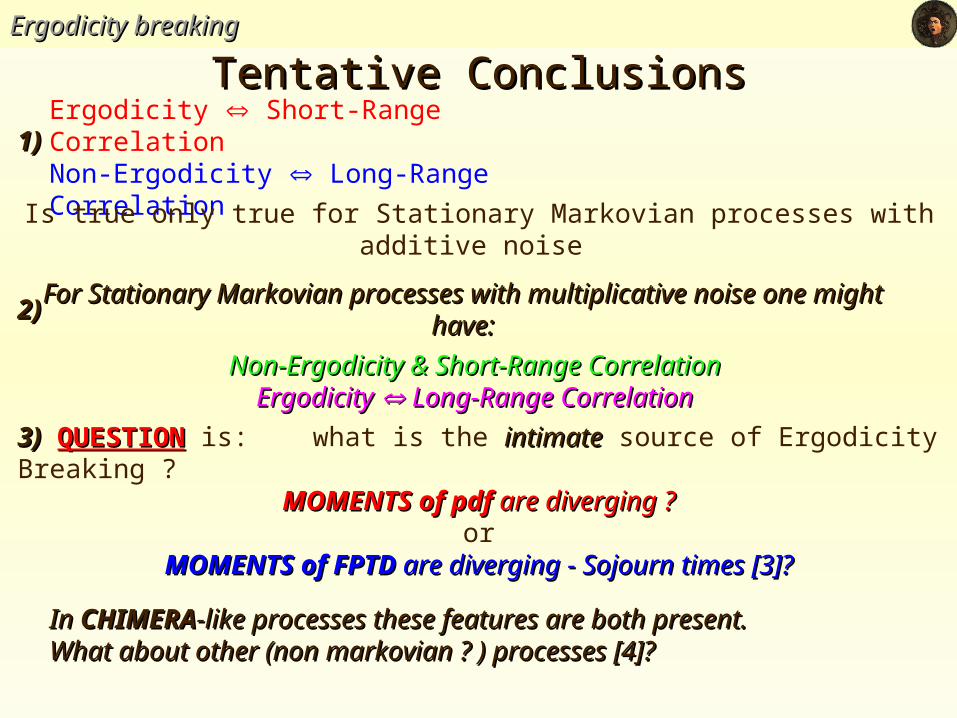
Tentative ConclusionsTentative ConclusionsErgodicity breakingErgodicity breaking
Ergodicity Short-Range CorrelationNon-Ergodicity Long-Range CorrelationIs true only true for Stationary Markovian processes with additive
noise
1)1)
For Stationary Markovian processes with multiplicative noise one For Stationary Markovian processes with multiplicative noise one might have:might have:2)2)
Non-Ergodicity & Short-Range Non-Ergodicity & Short-Range CorrelationCorrelation
Ergodicity Ergodicity Long-Range Correlation Long-Range Correlation
MOMENTS of pdfMOMENTS of pdf are diverging ? are diverging ?or
MOMENTS of FPTDMOMENTS of FPTD are diverging - Sojourn times [3]? are diverging - Sojourn times [3]?
3)3) QUESTIONQUESTION is: what is the intimateintimate source of Ergodicity Breaking ?
In In CHIMERACHIMERA-like processes these features are both present. -like processes these features are both present. What about other (non markovian ? ) processes [4]?What about other (non markovian ? ) processes [4]?
A Two-Region Stochastic Volatility ModelA Two-Region Stochastic Volatility Model
Part IIIPart III
EconoEcono PhysicsPhysics
from from -PHYSICS-PHYSICS to to ECONO-ECONO- (?) (?)
A Two-Region Stochastic Volatility ModelA Two-Region Stochastic Volatility Model
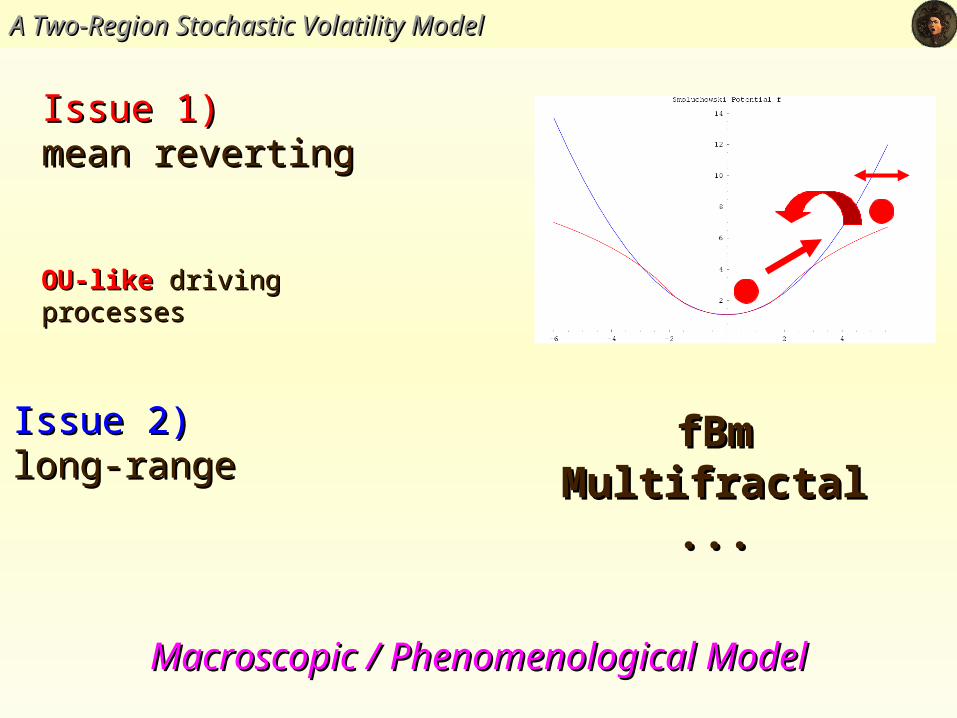
Issue 1)Issue 1) mean revertingmean reverting
OU-likeOU-like driving processes driving processes
Issue 2)Issue 2) long-rangelong-range
fBmfBmMultifractalMultifractal
......
Macroscopic / Phenomenological ModelMacroscopic / Phenomenological Model
A Two-Region Stochastic Volatility ModelA Two-Region Stochastic Volatility Model
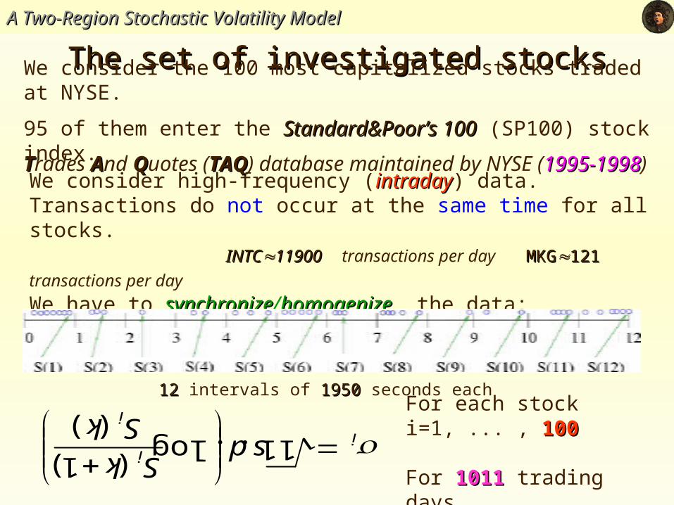
The set of investigated stocksThe set of investigated stocksWe consider the 100 most capitalized stocks traded at NYSE.
95 of them enter the Standard&Poor’s 100Standard&Poor’s 100 (SP100) stock index.
We consider high-frequency (intradayintraday) data. Transactions do not occur at the same time for all stocks. INTCINTC1190011900 transactions per day MKGMKG121 121 transactions per day We have to synchronizesynchronize/homogenizehomogenize the data:
) (
)1 (log . . 11
k S
k Sds
i
ii For each stock i=1, ... , 100100
For 10111011 trading days
1212 intervals of 19501950 seconds each
TTrades AAnd QQuotes (TAQTAQ) database maintained by NYSE (1995-19981995-1998)
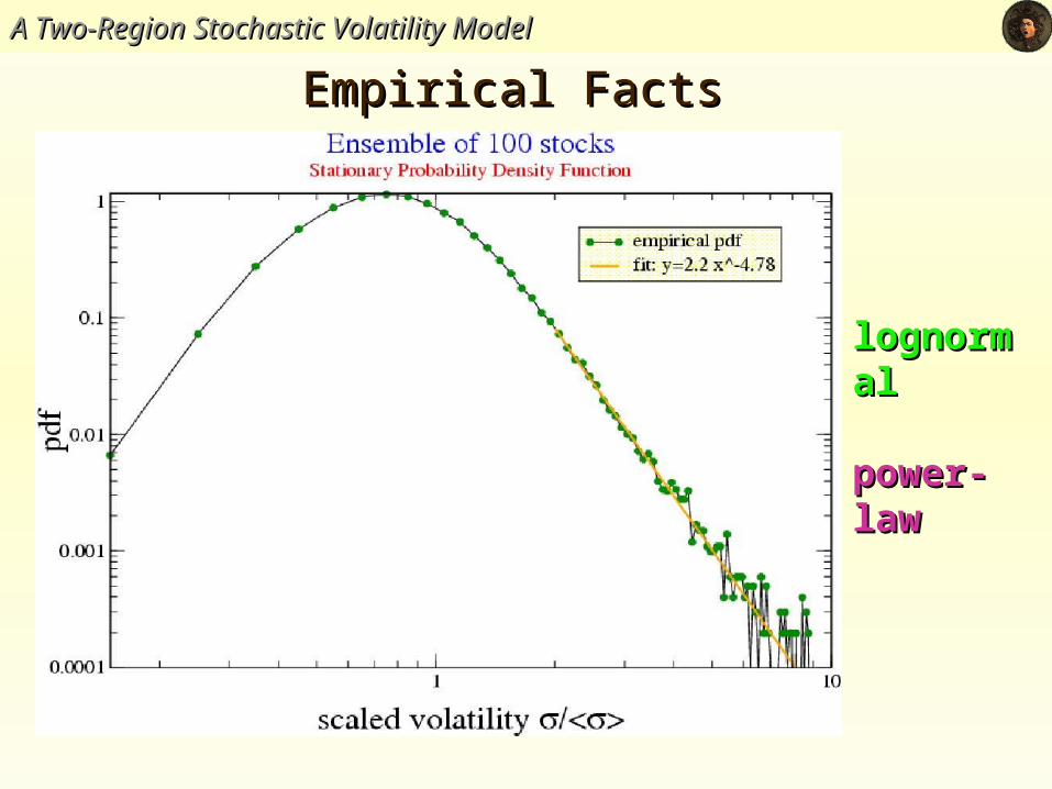
Empirical FactsEmpirical Facts A Two-Region Stochastic Volatility ModelA Two-Region Stochastic Volatility Model
lognormallognormal
power-lawpower-law

Empirical Facts Empirical Facts A Two-Region Stochastic Volatility ModelA Two-Region Stochastic Volatility Model
(()) --
0.30.3
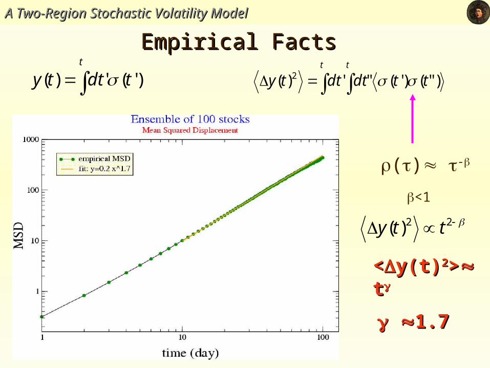
Empirical Facts Empirical Facts A Two-Region Stochastic Volatility ModelA Two-Region Stochastic Volatility Model
<<y(t)y(t)22>> t t
1.71.7
() -
<1
t
tdtty )'(')( t t
ttdtdtty )"()'("')( 2
22)( tty
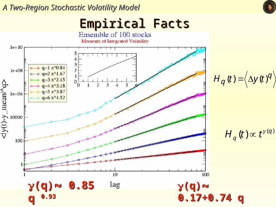
Empirical Facts Empirical Facts A Two-Region Stochastic Volatility ModelA Two-Region Stochastic Volatility Model
qq tytH )()(
)()( qq ttH
(q)(q) 0.17+0.74 0.17+0.74 qq
(q)(q) 0.85 q 0.85 q 0.930.93
Empirical Facts Empirical Facts A Two-Region Stochastic Volatility ModelA Two-Region Stochastic Volatility Model
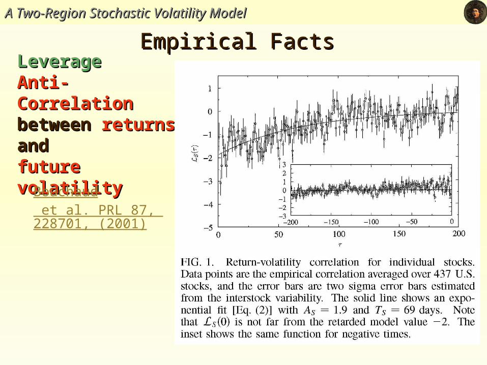
LeverageLeverage Anti-Correlation Anti-Correlation between between returnsreturns and and future volatility future volatility
Bouchaud et al. PRL 87, 228701, (2001)
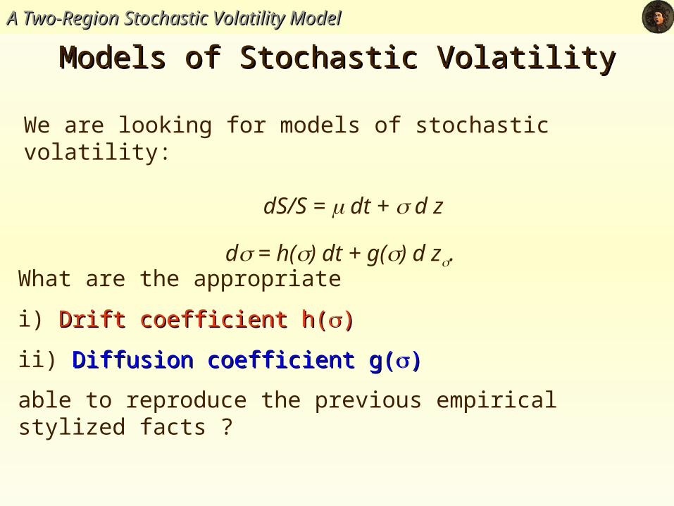
Models of Stochastic VolatilityModels of Stochastic VolatilityA Two-Region Stochastic Volatility ModelA Two-Region Stochastic Volatility Model
What are the appropriate
i) Drift coefficient h(Drift coefficient h())
ii) Diffusion coefficient g(Diffusion coefficient g())
able to reproduce the previous empirical stylized facts ?
We are looking for models of stochastic volatility:
dS/S = dt + d z
d = h() dt + g() d z.
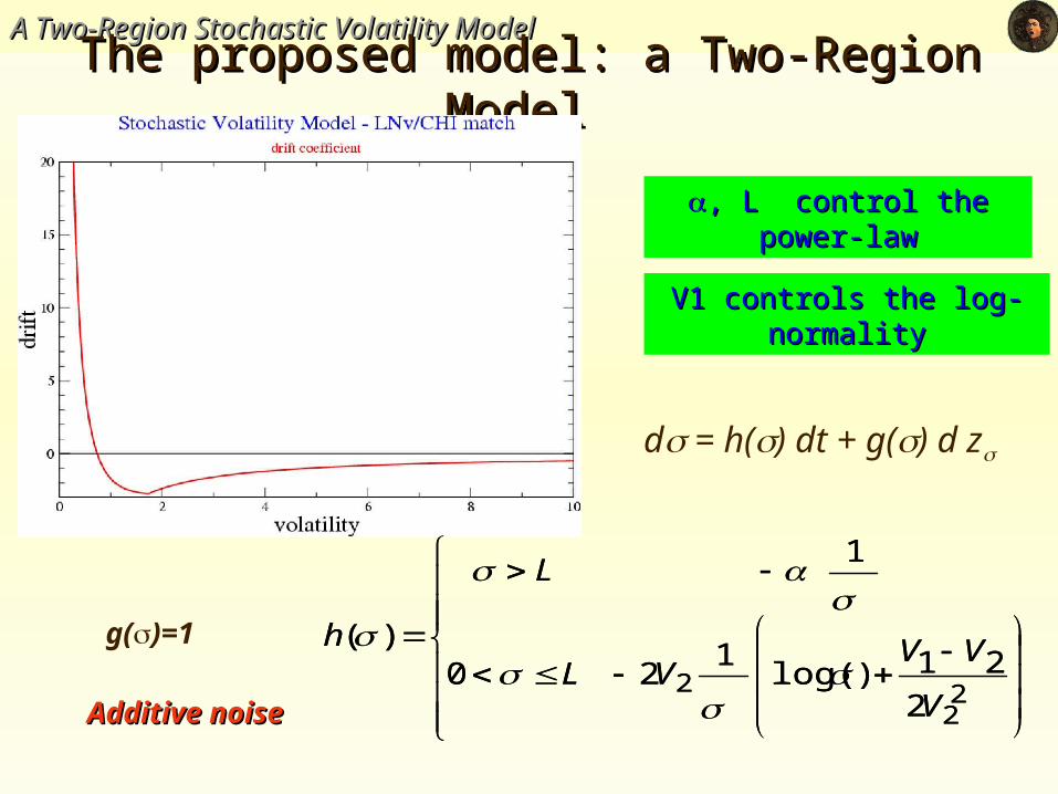
A Two-Region Stochastic Volatility ModelA Two-Region Stochastic Volatility Model
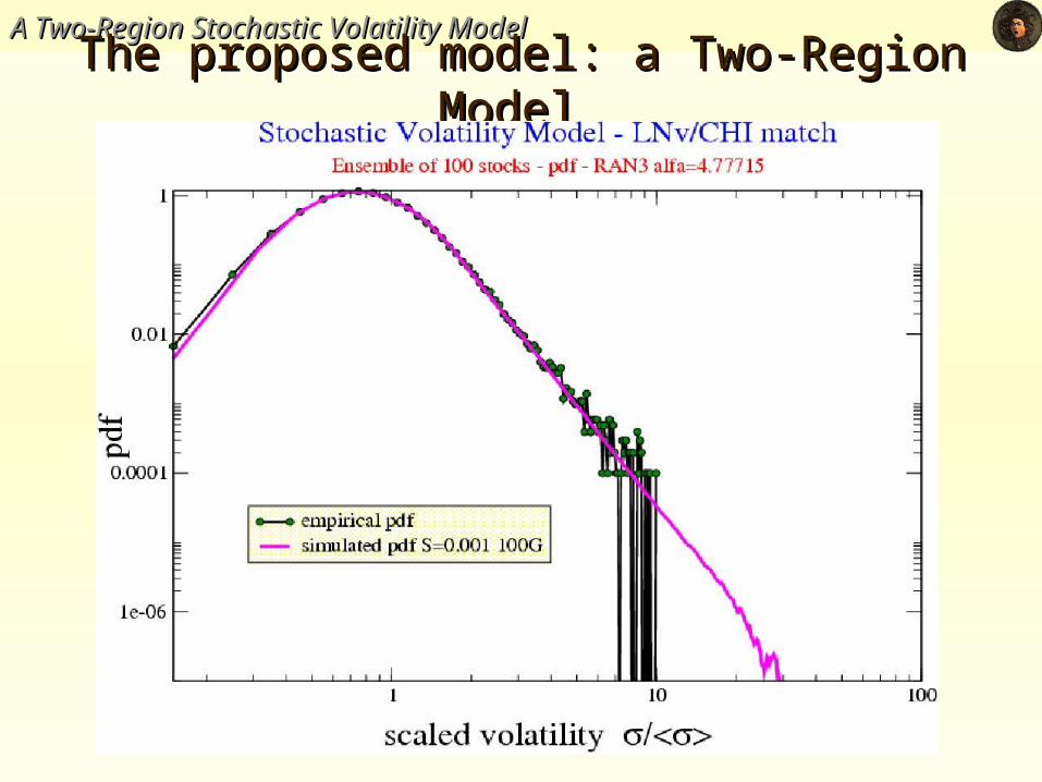
The proposed model: a Two-Region Model The proposed model: a Two-Region Model
22
22
21)log(1
20
1
)(
V
VVVL
L
h
g()=1
Additive noiseAdditive noise
, L control the power-, L control the power-lawlaw
V1 controls the log-V1 controls the log-normalitynormality
22
22
21)log(1
20
1
)(
V
VVVL
L
h
d = h() dt + g() d z
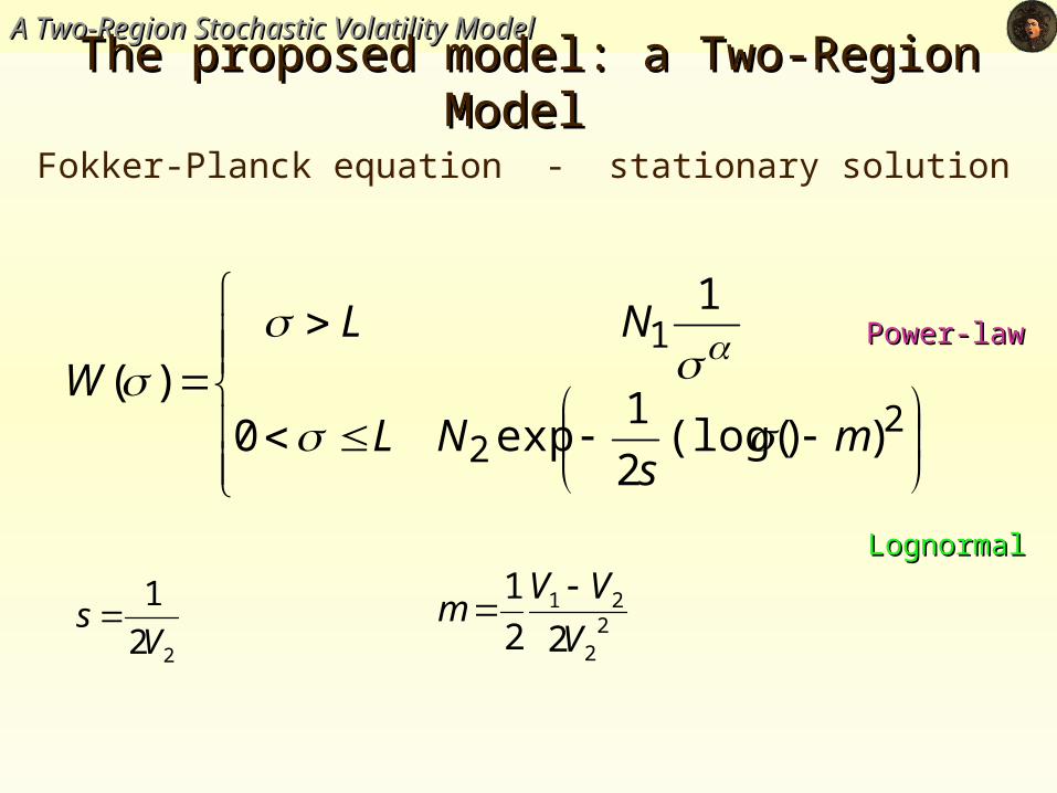
A Two-Region Stochastic Volatility ModelA Two-Region Stochastic Volatility Model
The proposed model: a Two-Region Model The proposed model: a Two-Region Model
22
1
))(log(2
1exp0
1
)(m
sNL
NLW
22
21
22
1
V
VVm
22
1
Vs
LognormalLognormal
Power-lawPower-law
Fokker-Planck equation - stationary solution
A Two-Region Stochastic Volatility ModelA Two-Region Stochastic Volatility Model
The proposed model: a Two-Region Model The proposed model: a Two-Region Model
A Two-Region Stochastic Volatility ModelA Two-Region Stochastic Volatility Model
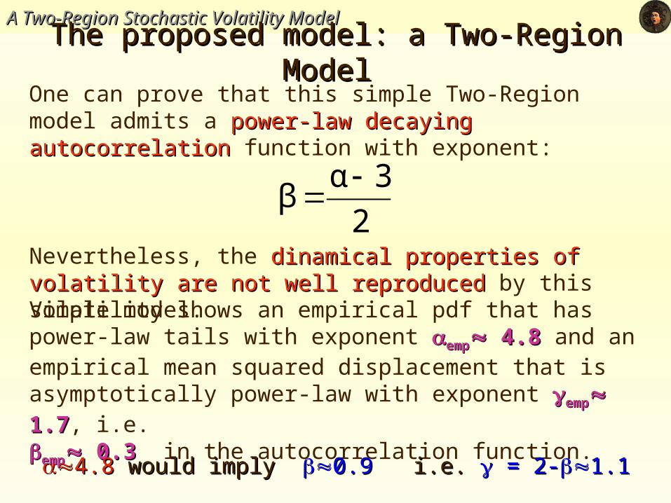
Nevertheless, the dinamical properties of volatility are not well dinamical properties of volatility are not well reproducedreproduced by this simple model.
The proposed model: a Two-Region Model The proposed model: a Two-Region Model
Volatility shows an empirical pdf that has power-law tails with exponent empemp 4.8 4.8 and an empirical mean squared displacement that is asymptotically power-law with exponent empemp 1.7 1.7, i.e.
empemp 0.3 0.3 in the autocorrelation function.
One can prove that this simple Two-Region model admits a power-power-law decaying autocorrelationlaw decaying autocorrelation function with exponent:
2
3αβ
4.8 4.8 would imply would imply 0.9 0.9 i.e.i.e. = 2- = 2-1.11.1
A Two-Region Stochastic Volatility ModelA Two-Region Stochastic Volatility Model
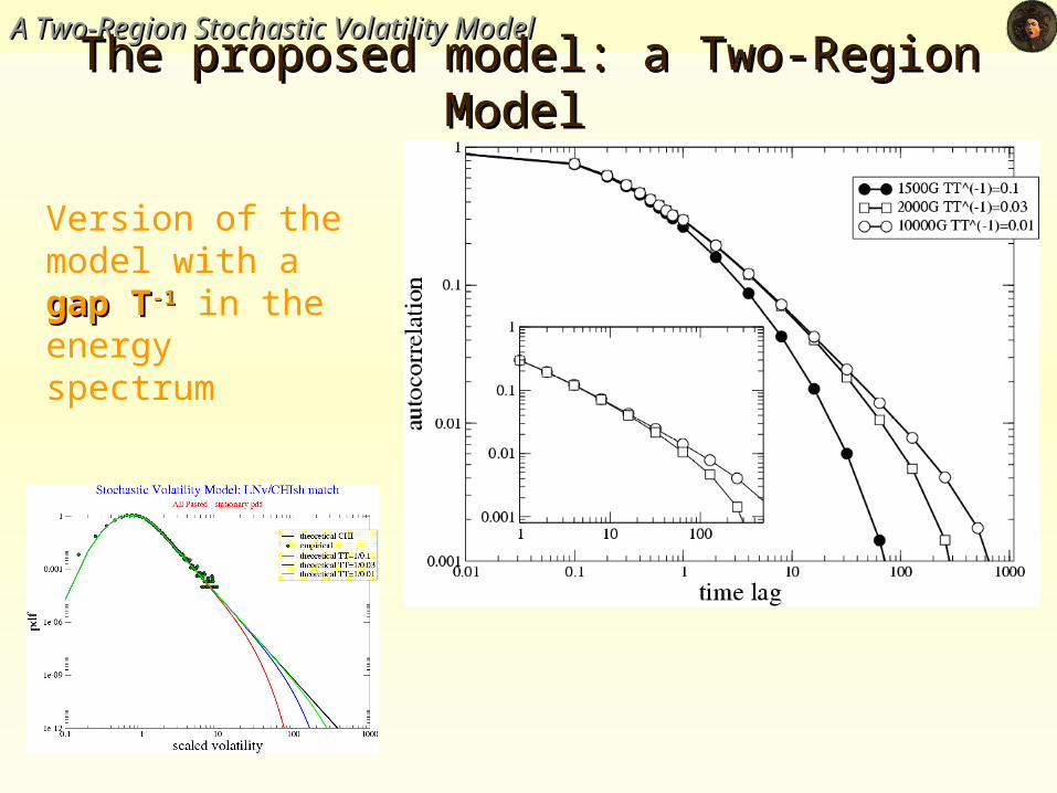
The proposed model: a Two-Region Model The proposed model: a Two-Region Model
Version of the model with a gapgap TT-1-1 in the energy spectrum
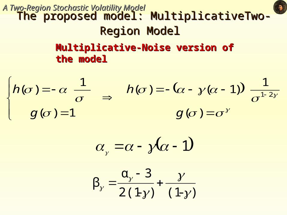
A Two-Region Stochastic Volatility ModelA Two-Region Stochastic Volatility ModelThe proposed model: MultiplicativeTwo-Region The proposed model: MultiplicativeTwo-Region
ModelModel
Multiplicative-Noise version of the modelMultiplicative-Noise version of the model
)-(1)-2(1
3αβ
)(
1)1()(
1)(
1)(
21
g
h
g
h
1
A Two-Region Stochastic Volatility ModelA Two-Region Stochastic Volatility Model
The proposed model: a Two-Region Model The proposed model: a Two-Region Model
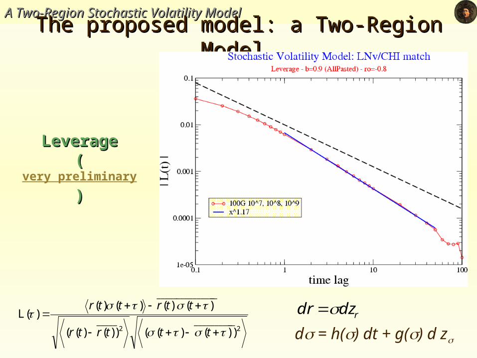
LeverageLeverage((very preliminary))
2___________
2_____
________________
))()(())()((
)()()()()(L
tttrtr
ttrttrrdzdr
d = h() dt + g() d z
A Two-Region Stochastic Volatility ModelA Two-Region Stochastic Volatility Model
ConclusionsConclusions
ReferencesReferences•S. Miccichè, G. Bonanno, F. Lillo, R. N. MantegnaS. Miccichè, G. Bonanno, F. Lillo, R. N. Mantegna , Physica A, , Physica A, 314314, , 756-761756-761, (2002), (2002)•S. Miccichè, G. Bonanno, F. Lillo, R. N. MantegnaS. Miccichè, G. Bonanno, F. Lillo, R. N. Mantegna , , Proceedings of: "The Second Nikkey Proceedings of: "The Second Nikkey Econophysics Research Workshop and Symposium", 12-14 November 2002, Tokio, Japan Econophysics Research Workshop and Symposium", 12-14 November 2002, Tokio, Japan Springer Verlag, Tokio, edited by H. Takayasu Springer Verlag, Tokio, edited by H. Takayasu
This simple model reproduces the empirical pdfempirical pdf quite well
The empirical Autocorrelation function is power-law. . The and exponents can be made independent from each other by generalizing the model as to considering a diffusion coefficient like g(g())
((multiplicative noise)).
The leverage effectleverage effect ...
The structure of smilestructure of smile, option pricingoption pricing, ...
A Two-Region Stochastic Volatility ModelA Two-Region Stochastic Volatility Model
Additional SlidesAdditional Slides
Stationary Markovian Stochastic Processes with Multiple Time-ScalesStationary Markovian Stochastic Processes with Multiple Time-Scales
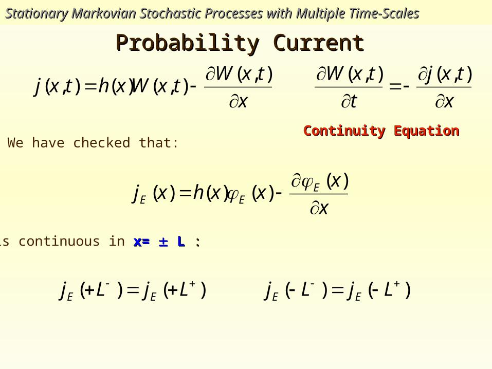
Probability Current Probability Current
x
txWtxWxhtxj
),(
),()(),(
We have checked that:
x
xxxhxj E
EE
)(
)()()(
is continuous in x= x= L L ::
)()( LjLj EE )()( LjLj EE
x
txj
t
txW
),(),(
Continuity EquationContinuity Equation
Stationary Markovian Stochastic Processes with Multiple Time-ScalesStationary Markovian Stochastic Processes with Multiple Time-Scales
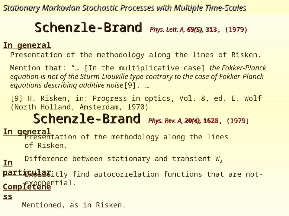
Schenzle-Brand Schenzle-Brand Phys. Rev. A, Phys. Rev. A, 20(4), 20(4), 16281628, (1979), (1979)
Completeness
In particular
Presentation of the methodology along the lines of Risken.
Difference between stationary and transient W2
Explicitly find autocorrelation functions that are not-exponential.
In general
Mentioned, as in Risken.
Schenzle-Brand Schenzle-Brand Phys. Lett. A, Phys. Lett. A, 69(5), 69(5), 313313, (1979), (1979)
Presentation of the methodology along the lines of Risken.
Mention that: “… [In the multiplicative case] the Fokker-Planck equation is not of the Sturm-Liouville type contrary to the case of Fokker-Planck equations describing additive noise[9]. …
[9] H. Risken, in: Progress in optics, Vol. 8, ed. E. Wolf (North Holland, Amsterdam, 1970)”
In general
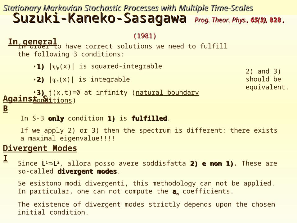
Stationary Markovian Stochastic Processes with Multiple Time-ScalesStationary Markovian Stochastic Processes with Multiple Time-ScalesSuzuki-Kaneko-Sasagawa Suzuki-Kaneko-Sasagawa Prog. Theor. Phys., Prog. Theor. Phys., 65(3), 65(3), 828828, ,
(1981)(1981) In general
Against S-B
Divergent Modes I
In order to have correct solutions we need to fulfill the following 3 conditions:
•1)1) |E(x)| is squared-integrable
•2)2) |E(x)| is integrable
•3)3) j(x,t)=0 at infinity (natural boundary conditions)
In S-B onlyonly condition 1)1) is fulfilledfulfilled.
If we apply 2) or 3) then the spectrum is different: there exists a maximal eigenvalue!!!!
2) and 3) should be equivalent.
Since LL11LL22, allora posso avere soddisfatta 2) e non 1)2) e non 1). These are so-called divergent modesdivergent modes.
Se esistono modi divergenti, this methodology can not be applied. In particular, one can not compute the aann coefficients.
The existence of divergent modes strictly depends upon the chosen initial condition.
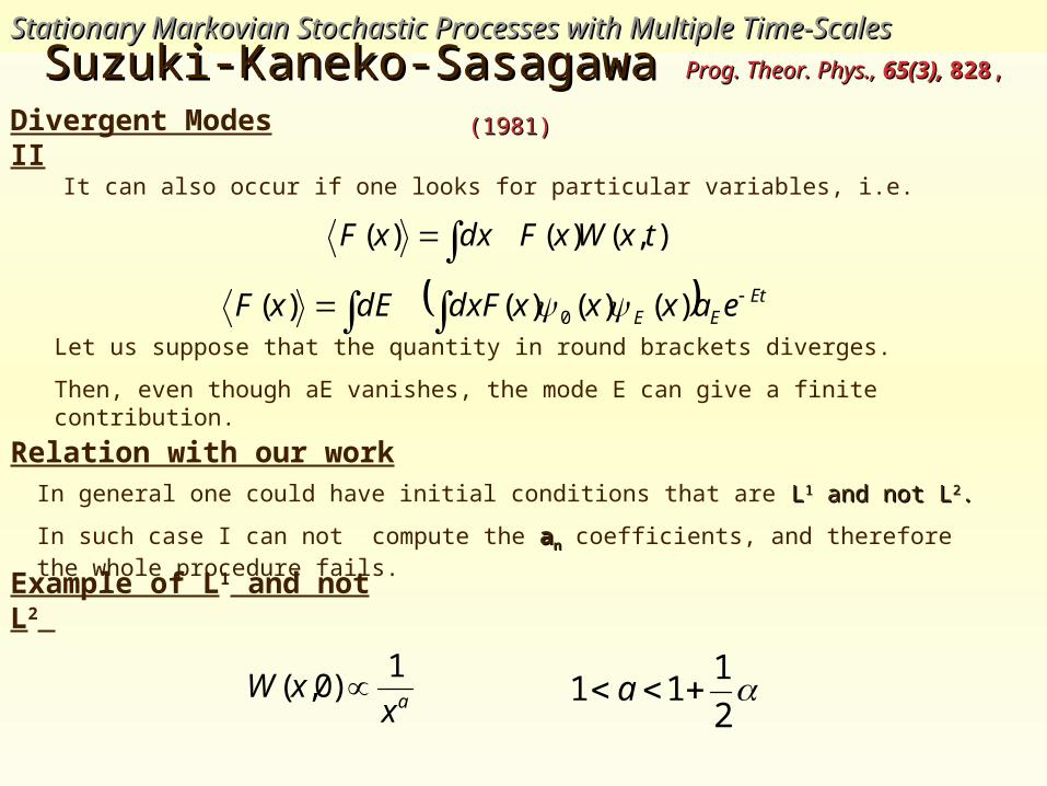
Stationary Markovian Stochastic Processes with Multiple Time-ScalesStationary Markovian Stochastic Processes with Multiple Time-ScalesSuzuki-Kaneko-Sasagawa Suzuki-Kaneko-Sasagawa Prog. Theor. Phys., Prog. Theor. Phys., 65(3), 65(3), 828828, ,
(1981)(1981)
Relation with our work
In general one could have initial conditions that are LL11 and not L and not L22..
In such case I can not compute the aann coefficients, and therefore the whole procedure fails.
Divergent Modes II
It can also occur if one looks for particular variables, i.e.
),()()( txWxFdxxF
EtEE eaxxxdxFdExF )()()()( 0
Let us suppose that the quantity in round brackets diverges.
Then, even though aE vanishes, the mode E can give a finite contribution.
Example of L1 and not L2
axxW
1)0,(
2
111 a
Stationary Markovian Stochastic Processes with Multiple Time-ScalesStationary Markovian Stochastic Processes with Multiple Time-Scales
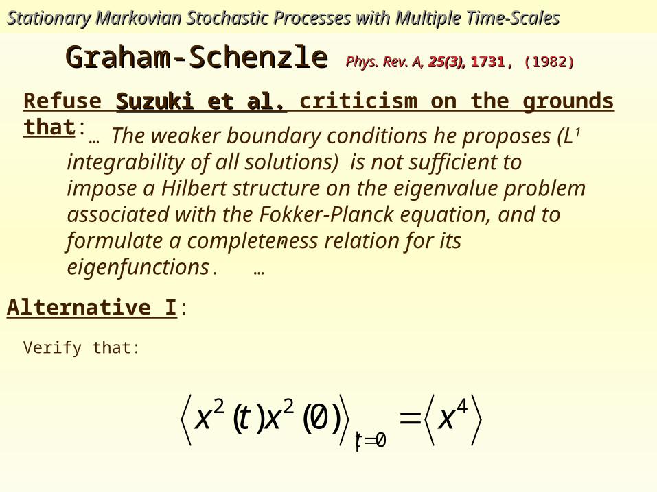
Graham-Schenzle Graham-Schenzle Phys. Rev. A, Phys. Rev. A, 25(3), 25(3), 17311731, (1982), (1982)
“ … The weaker boundary conditions he proposes (L1 integrability of all solutions) is not sufficient to impose a Hilbert structure on the eigenvalue problem associated with the Fokker-Planck equation, and to formulate a completeness relation for its eigenfunctions. …”
Verify that:
4
0|
22 )0()( xxtxt
Refuse Suzuki et al.Suzuki et al. criticism on the grounds that:
Alternative I:
Stationary Markovian Stochastic Processes with Multiple Time-ScalesStationary Markovian Stochastic Processes with Multiple Time-Scales
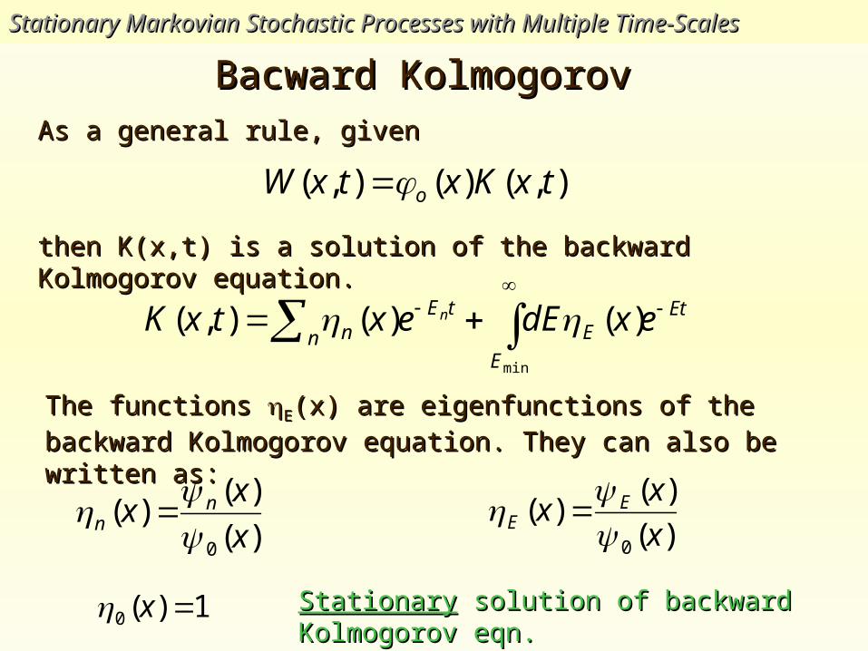
Bacward Kolmogorov Bacward Kolmogorov
),()(),( txKxtxW oAs a general rule, givenAs a general rule, given
)(
)()(
0 x
xx n
n
)(
)()(
0 x
xx E
E
1)(0 x StationaryStationary solution of backward Kolmogorov eqn. solution of backward Kolmogorov eqn.
then K(x,t) is a solution of the backward Kolmogorov equation.then K(x,t) is a solution of the backward Kolmogorov equation.
Et
E
En
tEn exdEextxK n
min
)()(),(
The functions The functions EE(x) are eigenfunctions of the backward Kolmogorov (x) are eigenfunctions of the backward Kolmogorov
equation. They can also be written as:equation. They can also be written as:


![N. Mantegna arXiv:1107.3942v1 [q-fin.TR] 20 Jul 2011 of](https://img.pdfslide.us/doc/110x75/625414675af99c695a7ba41d/n-mantegna-arxiv11073942v1-q-fintr-20-jul-2011-of-.jpg)