SOME NOVEL DEVELOPMENTS IN FINITE ELEMENT PROCEDURES … · international journal for numerical methods in engineering, vol.39, 2477-2505 (1996) some novel developments in finite

Some novel developments in finite element proceduresfor gradient-dependent plasticityde Borst, R.; Pamin, J.

Published in:International Journal for Numerical Methods in Engineering

DOI:10.1002/(SICI)1097-0207(19960730)39:14<2477::AID-NME962>3.0.CO;2-E

Published: 01/01/1996

Document VersionPublisher’s PDF, also known as Version of Record (includes final page, issue and volume numbers)

Please check the document version of this publication:

• A submitted manuscript is the author's version of the article upon submission and before peer-review. There can be important differencesbetween the submitted version and the official published version of record. People interested in the research are advised to contact theauthor for the final version of the publication, or visit the DOI to the publisher's website.• The final author version and the galley proof are versions of the publication after peer review.• The final published version features the final layout of the paper including the volume, issue and page numbers.

Link to publication

General rightsCopyright and moral rights for the publications made accessible in the public portal are retained by the authors and/or other copyright ownersand it is a condition of accessing publications that users recognise and abide by the legal requirements associated with these rights.

• Users may download and print one copy of any publication from the public portal for the purpose of private study or research. • You may not further distribute the material or use it for any profit-making activity or commercial gain • You may freely distribute the URL identifying the publication in the public portal ?

Take down policyIf you believe that this document breaches copyright please contact us providing details, and we will remove access to the work immediatelyand investigate your claim.

Download date: 25. Aug. 2018

https://doi.org/10.1002/(SICI)1097-0207(19960730)39:14<2477::AID-NME962>3.0.CO;2-E

https://research.tue.nl/en/publications/some-novel-developments-in-finite-element-procedures-for-gradientdependent-plasticity(6f15af10-bfdf-4c54-ac2f-be6815591f97).html

INTERNATIONAL JOURNAL FOR NUMERICAL METHODS IN ENGINEERING, VOL. 39, 2477-2505 (1996)

SOME NOVEL DEVELOPMENTS IN FINITE ELEMENT PROCEDURES FOR GRADIENT-DEPENDENT PLASTICITY

RENE DE BORST* AND JERZY PAMIN'

Dew University of Technology, Faculty of Civil Engineering, P.O. Box 5048,2600 G A Dew, The Netherlands

SUMMARY Improved algorithms are proposed for a gradient plasticity theory in which the Laplacian of an invariant plastic strain measure enters the yield function. Particular attention is given to the type of finite elements that can be used within the format of gradient-dependent plasticity. Assuming a weak satisfaction of the yield function, mixed finite elements are developed, in which the invariant plastic strain measure and the displacements are discretized. Two families of finite elements are developed: one in which the invariant plastic strain measure is interpolated using C '-continuous polynomials, and one in which penalty-enhanced C'continuous interpolants are used. The performance of both families of finite elements is assessed numerically in one-dimensional and two-dimensional boundary value problems. The regularizing effect of the used gradient enhancement in computations of elastoplastic solids is demonstrated, both for mesh refinement and for the directional bias of the grid lines.

KEY WORDS higher-order continua; plasticity; localization; mixed elements

1. INTRODUCTION

Conventional constitutive models which incorporate strain softening tend to exhibit an extreme mesh sensitivity when numerical methods are applied to the solution of boundary value problems. The introduction of strain softening triggers localized zones of high strain intensity. In standard, rate-independent continuum models, the size of these localization zones is not specified and is therefore fully determined by the discretization. Also, the direction of the localization zones is biased by the mesh lines. The underlying reason is the fact that the set of governing partial differential equations can locally change type at the onset of strain softening. Whether this indeed occurs depends on the applied constitutive model and the particular boundary value problem.

Upon the emergence of a localization zone, the standard, rate-independent continuum model together with the equilibrium equations and the kinematic relations no longer results in a set of partial differential equations that is elliptic under static loading conditions. Instead, locally the set of equations becomes hyperbolic, which allows for the occurrence of discontinuities in the strain distribution. As a consequence localization of deformation can take place in a set of measure zero (a line in two-dimensional configurations and a plane in three-dimensional problems). The finite element solution attempts to reproduce this discontinuity by a localization band that is between one and two elements wide, depending on the angle between the propagation direction of the localization band and the grid lines.

* Also at Eindhoven University of Technology, Faculty of Mechanical Engineering 'On leave from Cracow University of Technology, Faculty of Civil Engineering

CCC 0029-5981/96/142477-29 0 1996 by John Wiley & Sons, Ltd.

Received 15 December 1994 Revised 24 July 1995

2478 R. DE BORST AND J. PAMIN

Various approaches have been suggested to avoid this change of character of the governing set of partial differential equations.' - Herein gradient plasticity is explored for this purpose.4- lo

Specifically, a theory is utilized in which the yield function depends on second-order spatial derivatives of an invariant plastic strain measure. This dependence introduces an internal length scale in the continuum model, which defines the width of the localization band and preserves ellipticity until far into the softening regime.

From a physical point of view, one can associate the occurrence of higher-order gradients in the macroscopic constitutive model with the non-local interaction between microstructural deformation carriers. Alternatively, gradient plasticity may be thought of as an approximation to fully non-local plasticity model^.'^^^ " 9 l 2 H owever, the physical justification of the introduction of higher-order deformation gradients is not the prime concern of this contribution, as an abund- ance of arguments exists in the literature in support of t h i ~ . ~ , ~ , ' ' Rather, we shall focus on the computational implications which result from the introduction of higher-order gradients of the inelastic strain in the constitutive description.

Due to the gradient dependence of the yield function, the consistency condition, which governs the plastic flow, becomes a partial differential equation. A possibility is to satisfy the yield condition in a distributed sense and to discretize the plastic strain field in addition to the usual discretization of the displacement^.'.^ Previous work includes a general formulation and an algorithm for gradient plasticity theory' and some applications to soil instability and concrete fracture.' ' This paper can be considered as an extension to and an improvement on the material presented in Reference 9, in the sense that a new family of elements is derived with Co-continuous interpolation functions, suitable for gradient plasticity, and that an improved algorithm for the stress computation is presented, including the derivation of a consistent tangent operator.

2. GRADIENT-DEPENDENT PLASTICITY

We start the discussion by briefly summarizing the rate boundary value p r ~ b l e m . ~ . ' ~ We introduce the displacement vector u = (ux, uy, u,), the strain tensor in a vector form E = ( E ~ ~ , cyy , E,,, yxy, yyz , yZx) and the stress tensor in a vector form ts = (oxx, oYy, o,,, oxy, oyz, orx). Under the assumption of small deformations and static loadings we have the following equations for an elastoplastic body occupying a volume I/:

LTI = 0 (1)

& = LU

ir = ~ " ( 1 : - dm)

where superimposed dots denote the derivative with respect to time and the superscript T is the transpose symbol. In the above equations L is a differential operator matrix and D" is the elastic stiffness matrix. Body forces have been skipped in equation (1) for simplicity. Equation (3) contains the definition of the plastic strain-rate vector, called the flow rule:

i p = jm (4)

in which is a plastic multiplier and m defines the direction of the plastic flow. The vector m may be derived from a plastic potential function G: m = aG/da.

The gradient dependence is included in the definition of the yield function F :

F = F ( c , K , V ? I C ) (5 )

NOVEL DEVELOPMENTS IN FINITE ELEMENT PROCEDURES 2479

in which u is an invariant plastic strain measure (hardening parameter). Together with equations (1H3) the Kuhn-Tucker conditions

X30, F<O, X F = O (6) must be fulfilled. To complete the rate boundary value problem we specify the standard static and kinematic boundary conditions on complementary parts of the body surface S:

cv, = t, u = us (7)

where X is the stress tensor in a matrix form, v, denotes the outward normal to the surface S and t is the boundary traction vector. It is noted that when the equation of motion is used instead of the equilibrium equation (l), and when appropriate initial conditions are supplied, an initial value problem can be formulated for dynamic loading^.^' l4

The gradient dependence of the yield function makes the plastic consistency condition P = 0 become a differential equation:

(gy6 + & aF li: + Fu aF V2K = 0

We introduce the gradient of the yield function n:

aF n = - aa

the (variable) hardening modulus h:

K aF h(lc,V21c) = - T-

Iz alc

and the gradient influence variable g:

ic aF g(u) = T-

,I avZK

(9)

which is assumed to be a function of K only. We limit our consideration to the theories of plastic flow, for which we can write

k = g A (12) with q a positive constant. This relation is broad enough to encompass the Huber-Mises, Drucker-Prager and Rankine yield functions with some form of strain hardening hypothesis. Then, we can write equation (8) in the form

nT6 - h i + g V z i = 0 (13) The partial differential equation (13), which must hold in the plastic part of the body V,, is characteristic for the present theory. For softening the modulus h is negative and the additional variable g must be positive. For g = 0 the classical flow theory of plasticity is retrieved. Then, the consistency condition is a non-linear algebraic equation, from which the plastic multiplier can be determined locally.

In this contribution we focus attention on the Huber-Mises gradient plasticity model, for which the yield function can be written in the following format:

F = f i - *#(K, v2K) (14)


with J z the second invariant of the deviatoric stress tensor and Og the (non-negative) yield strength. Introducing a symmetric matrix P,

3 3 1 - 3 0 0 0 _ - 1 2 _ - : o o o _ - 1 _ - I 5 0 0 0

- 2 - _ - 3 3

3 3

0 0 0 2 0 0

0 0 0 0 2 0

- 0 0 0 0 0 2

the function F can be written in the following form:

so that the gradient to the yield function equals

To determine the relation between k and 2 we adopt the strain-hardening hypothesis:

(18) r;: = (3k!’.iP.)1/2 = [$(iP)TQiP]3”2 1J II

with Q = diagC1, 1, 1, f, 9, f]. For an associated flow rule, the plastic strain rate is given by i p = An. Substitution of this identity into the definition of k and noting that PQP = P leads to

k = 1 , q = l (19)

The important advantage of the Huber-Mises yield function is its smoothness, since the presence of singular edges on the yield surface poses a difficulty for the gradient plasticity a1g0rithm.I~

3. INCREMENTAL FORMULATION

In order to derive an incremental-iterative algorithm for gradient plasticity, we require a weak satisfaction of the equilibrium condition9~’

and the yield condition

at the end of iterationj + 1 of the current loading step, where b denotes a variation of a quantity. Equation (20) can be modified using integration by parts and the standard boundary condi-

tions (7)1y and decomposing oj+ as aj + du, where d indicates an increment, i.e. the difference between the values of a variable at the end of iterationj + 1 and iteration j:

J 6zTdodV = J 6uTtj+l dS - 6ETujdV V S J V

NOVEL DEVELOPMENTS IN FINITE ELEMENT PROCEDURES 248 1

Using the incremental form of the relationship between the stress vector and the elastic strain vector

d a = D’(ds - d lm) (23)

we obtain the following integral equation:

Sy6sTDe(ds - dAm)dV = ss 6uTtj+l dS - jv6sTujdV (24)

We observe that this equation does not depend explicitly on the Laplacian of the plastic multiplier and has a form similar to the incremental equilibrium equations used for classical plasticity.

Strictly speaking, relation (23) and therefore also the ensuing equation hold for infinitesimally small changes of stress and strain. If a return mapping algorithm is used to integrate the rate equations, the resulting set of equations can be differentiated for consistent linearization, again yielding an equation of the form (23), but with the elastic stiffness matrix D‘ replaced by an algorithmic stiffness matrix H, see Section 6.2.

The yield function F in equation (21) is developed in a Taylor series around (aj, K ~ , V’K~) and truncated after the linear terms. With the definitions (9Hll) we obtain

F ( C ~ + ~ , K ~ + ~ , V ’ K ~ + ~ ) = F ( u ~ , K ~ , V ’ K ~ ) + nTda - h d l + gV’(dL) (25)

which, after substitution into equation (21), results in

61[nTD’da - (h + nTD‘m)dl + gV’(dl)]dV = - 61F(aj, KjrVZKj)dl/ (26)

The values of n, m, h and g on the left-hand side of equation (26) are determined at the end of iterationj, i.e. for the state defined by (aj, I C ~ , V’K~). Using integration by parts for the last term on the left-hand side of equation (26) we obtain

J:

r r r ! 6A[oTD’ds - (h + nTD‘m)dA]dV - ! g(V6A)T(VdL)dV = - 6AF(uj,Kj.V2Kj)dV VA V1 J V *

provided the non-standard boundary conditions

6 A = O or (Vdl)Tvrl=O (28)

are fulfilled on the whole boundary S1 of the plastic part of the body. The first condition is delicate for finite increments, since the elastic-plastic boundary moves when the plastic zone in the body evolves. During this process the boundary condition 82 = 0 on the momentary elastic-plastic boundary may not be true and (28), must hold. If the same mesh is used for both the equilibrium and yield condition, i.e. if integrals over the whole volume V appear in equations (21) and (26)/(27), either the admissible d l must vanish or we must enforce F = 0, n = m = 0 and d 1 = 0 in the elastic part of the body.

The dependence of the yield function on the Laplacian of the plastic strain measure is essential for the plastification condition and for the calculation of the non-standard residual forces on the right-hand side of equations (26)/(27). To enable expansion of the plastic process from the


originally imperfect zones, the numerical solution must correctly determine a positive value of the Laplacian at the elastic-plastic boundary. The boundary conditions (28)2 require the existence of derivatives of 1 as nodal degrees of freedom. Therefore C'-continuous interpolation functions are necessary for 1 whether equation (26) or equation (27) is di~cretized.'~ This issue has raised some doubts in the past,' since the formulation of the variational principle for gradient plasticity' suggests that the use of a standard Co-interpolation for the plastic multiplier is sufficient.

4. REMARKS ON C'-CONTINUOUS FORMULATION

In the integral equations (24) and (26)/(27) there appear at most first-order derivatives of the displacements and second-order derivatives of the plastic multiplier. Therefore, the discretization of the displacement field u requires Co-continuous interpolation functions N and the discretization of the plastic multiplier 1 requires C'-continuous shape functions h:

u = N a , I = h T A (29)

where a is a nodal displacement vector and A denotes a vector of nodal degrees of freedom for the plastic multiplier field. The strain vector E can then be written as

E = Ba (30)

where B = LN according to the linear kinematic relation (2). The gradient of the plastic multiplier VA and the Laplacian of the plastic multiplier Vz 1 are then discretized as follows:

V 1 = qTA, V 2 1 = pTA (3 1)

where qT = VhT and p contains the Laplacians of the C'-continuous interpolation functions in h. Discretizing the integral equations (24) and (26) using equations (29H31) and requiring that the result holds for all admissible 6a and 6A, one arrives at a non-linear algebraic set of equations'

with the elastic stiffness matrix

K,,= BTDeBdV I (33)

the off-diagonal matrices

BTDemhTdV, KA, = - (34)

the gradient-dependent matrix

[(h + nT Dem) hhT - g hpT] d Y (35)

and the vectors

N'tj+ldS, f a = - F(aj,Ij,V21j)hdV


respectively. The matrix KAA is non-symmetric due to the gradient dependence even for an associated flow rule as considered here (m = n). If equation (27) is used as a point of departure instead of equation (26) the matrix KA1 becomes symmetric:

[(h + nTD'm)hhT + gqqT] dV (37)

With respect to the non-standard boundary conditions for the plastic multiplier field, we notice that both boundary conditions (28) are satisfied at the evolving elastic-plastic boundary if C'-continuity is satisfied. However, the second of the conditions (28) must be enforced on the outer boundary of the plastic part or, in practice, on the whole surface of the body if the tangent operator in equation (32) is symmetric or if it does not possess a sufficient rank for elastic elements. To illustrate this point we consider a structure which is initially elastic and then, due to an inhomogeneous stress distribution, exhibits a partial plastification. If all elements are elastic, we have K1, = 0 since the gradient vectors m and n are set to zero. Then we obtain from equation (32) the classical set of equations in da

K,,,da = f, + fa (38)

and the additional set of equations in dA

For the elastic state we have F <O and we set the residual forces f, to zero. Equation (39) then yields the desired solution dA = 0 if the global matrix Ki, is non-singular after the element assembly and, if necessary, after the introduction of boundary conditions for the A degrees of freedom. If plastic elements appear in the structure, we have f, # 0 in elastic elements adjacent to the plastic zone and we compute non-zero dA from equation (39).

To avoid singularity of the tangent operator for elastic elements the hardening modulus h in equation (35) is initially set equal to Young's modulus E. The gradient term may be neglected in the matrix K:, for elastic elements as its inclusion only slightly influences the results. Using numerical integration the matrix Ki, is then determined as

where Vi is a volume contribution of an integration point. The rank of submatrix K;, should be examined in order to determine the number of integration points and additional boundary conditions necessary to avoid spurious kinematic modes for the plastic multiplier field.

On the other hand, a high-order integration scheme and too many additional boundary conditions of the A field can lead to an overconstrained plastic flow and have a negative influence on the accuracy of finite element predictions. Since the yield condition can be conceived as a differential constraint to the equilibrium condition of a non-linear solid, the number of constraints for the plastic multiplier field must be limited, otherwise the solution will be inaccurate or will lock, just as happens for some standard elements under isochoric deformations. In other words, we have a two-field theory similar to the mixed formulation with independent displacement and pressure interpolation and a proper constraint ratio between the displacement and R degrees of freedom should be satisfied.


5. Co-FORMULATION WITH A PENALTY CONSTRAINT

In order to be able to use Co-continuous interpolation functions for the plastic multiplier field, we introduce new variables cpx, cpy and cp,:

and collect them in a vector + = (cpx, cpy , cp,). In this fashion we can write the gradient of the plastic mu!tiplier as

V A = + (42)

and represents the Laplacian of I as

where the scalar product of the operator VT and the vector field + denotes the divergence operator. The result of equation (43) can be substituted in equation (26) or (27), but the constraint (42) must be added to the formulation.

Since we want to avoid the introduction of a Lagrangian multiplier field in addition to the introduced fields u, 1 and Q,, we make use of a penalty approach. We include the constraint by means of an additional variational equation:

where k is a penalty factor. In practical calculations we use k = E3, where E is Young's modulus. Using the incremental form of equation (44) together with equations (24) and (26) we obtain a set of three integral equations:

J 6ETDe(d& - dAm)dV = 6uTtj+, dS - J GETujdV (45) V V

jv61[nTWd& - (h + nTDem)dA + gVTd+]dV = - 61F(uj, ~ ~ , V ~ i ~ ~ ) d i / (46) J-V

where according to equations (12) and (43) we calculate V'K = qVT+ and

k 61VT[V(dI) - d+] dV - k S+'[V(dn) - d+] dV = 0 (47) J: IV The above equations are now discretized using Co-continuous interpolation functions. The interpolation functions for the displacement field are like in the previous section, but the shape functions h for the plastic multiplier field in equation (29)~ are now Co-continuous. The following interpolation for the new variables in Q, is used:

+=P@ (48)


where @ contains the nodal values of 'px, 'p,, and 'pz and P is a matrix of shape functions, similar to N in equation (29),. Upon the discretization of equations (45H47) and the usual argument that the resulting equations

r r r

haT J [BTDeBda - BTD'mhTdA]dV = daT NTtj+ldV - SaT J BTajdV (49) V V

dATjv[ - hnTDeBda + (h + nTDem)hhTdA - ghVTPd@]dV = 6AT F(aj, K ~ , V ' K ~ ) ~ ~ V I and

kGAT J q(qTdA - Pd@)dV - k6mT PT(qTdA - Pd@)dV = 0 V J Y

must hold for any admissible Sa, 6A and 6@, we obtain the following set of algebraic equations in a matrix form:

where K,,, Kan and K,, are given in equations (33) and (34), K1, and K, are defined as r r

Knn = (h + nTDem)hhTdV, KI, = - [ghVTP] dV J v J v (53)

and the submatrices with the superscript c in the additional (symmetric) matrix introducing the constraint (42) are defined as

I

Kf;, = qqTdV, K & = j vPTPdV, K;, = jv - qPdV b (54)

As in the preceding section, due to the gradient dependence the tangent operator in equation (52) is non-symmetric.

If we substitute the definitions (42) and (43) into equation (27), instead of into equation (26), the symmetric formulation of the tangent stiffness matrix ensues. In particular, we obtain the weak form of the yield condition as

r r r

6,1[nTDedE -(h + nTDem)dl]dV - gS+d+dV = - dAF(aj, Kj,V2Kj)dV (55) JV JV JV

in which the derivatives of + appear only on the right-hand side in V'K~. Substitution of equations (29),, (30) and (48) gives the second form of the discretized yield condition:

dATSv[ -hnTDcBda + ( h + nTDem)hhTdA]dV + gdcDTPTPd@dV SV


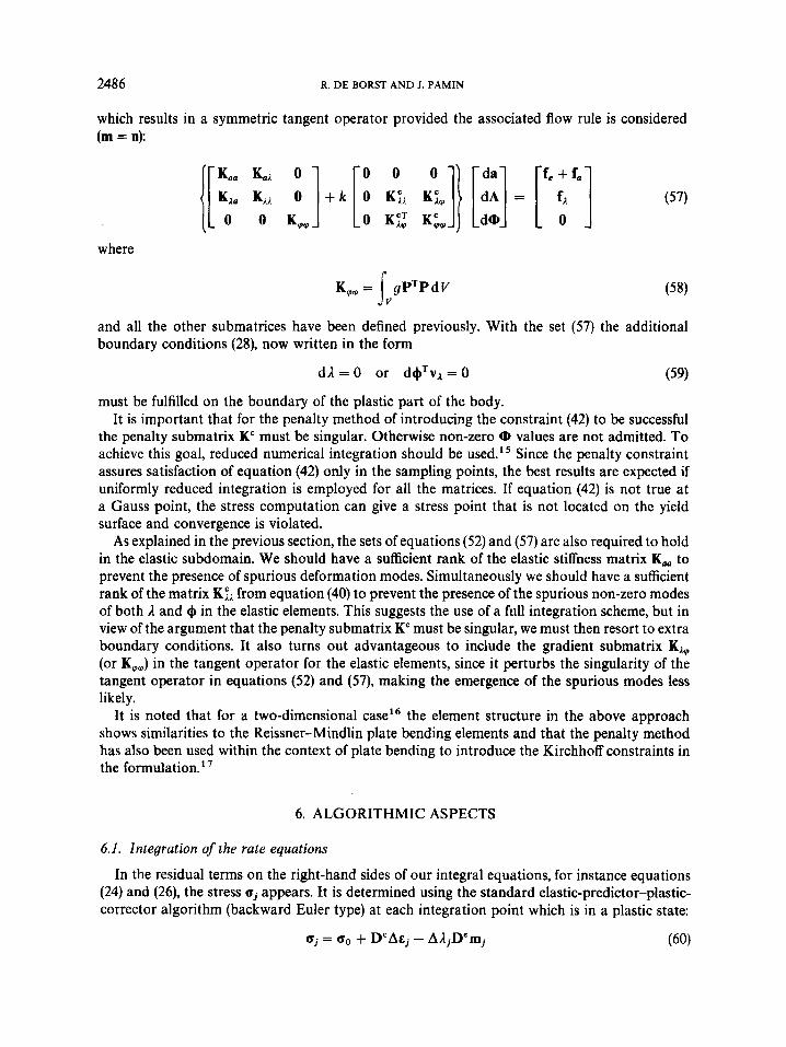
which results in a symmetric tangent operator provided the associated flow rule is considered (m = 0):

where

K,,= gPTPdV b and all the other submatrices have been defined previously. With the set (57) the additional boundary conditions (28), now written in the form

dA=O or d$'vA=O (59)

must be fulfilled on the boundary of the plastic part of the body. It is important that for the penalty method of introducing the constraint (42) to be successful

the penalty submatrix K" must be singular. Otherwise non-zero 8 values are not admitted. To achieve this goal, reduced numerical integration should be used." Since the penalty constraint assures satisfaction of equation (42) only in the sampling points, the best results are expected if uniformly reduced integration is employed for all the matrices. If equation (42) is not true at a Gauss point, the stress computation can give a stress point that is not located on the yield surface and convergence is violated.

As explained in the previous section, the sets of equations (52) and (57) are also required to hold in the elastic subdomain. We should have a sufficient rank of the elastic stiffness matrix K,, to prevent the presence of spurious deformation modes. Simultaneously we should have a sufficient rank of the matrix K:A from equation (40) to prevent the presence of the spurious non-zero modes of both 3, and $ in the elastic elements. This suggests the use of a full integration scheme, but in view of the argument that the penalty submatrix K" must be singular, we must then resort to extra boundary conditions. It also turns out advantageous to include the gradient submatrix K, (or KVV) in the tangent operator for the elastic elements, since it perturbs the singularity of the tangent operator in equations (52) and (57), making the emergence of the spurious modes less likely.

It is noted that for a two-dimensional case' the element structure in the above approach shows similarities to the Reissner-Mindlin plate bending elements and that the penalty method has also been used within the context of plate bending to introduce the Kirchhoff constraints in the formulation. l 7

6. ALGORITHMIC ASPECTS

6.1. Integration of the rate equations

In the residual terms on the right-hand sides of our integral equations, for instance equations (24) and (26), the stress aj appears. It is determined using the standard elastic-predictor-plastic- corrector algorithm (backward Euler type) at each integration point which is in a plastic state:

aj = a,, + D'Azj - AljD'mj (60)


where a. is the stress state at the end of the previous (converged) load increment and A denotes a total increment (from state 0 to iterationj). The values of K~ and V21cj are also updated using total increments. Since the vector mj is known only after the mapping in equation (60), it is approximated by the gradient m, calculated for the 'trial' stress:

= GO + DCA&j (61) To decide whether an elastic point enters the plastic regime, or whether a plastic point begins elastic unloading the trial value of the yield function F, is calculated at each integration point:

Ft = F(at, 8g(Kj,VzKj)) (62)

5, = (T(Kj) - g(Kj)vz l j (63)

where the gradient-dependent yield strength 5, is determined as follows:

An integration point is assumed to be in the plastic state when F, > O and in the elastic state when F, <O. In the elastic elements I = 0, so that for spreading of the plastic zone it is crucial that the numerical solution allows V21 > 0 at the elastic-plastic boundary. The gradient-dependent yield strength 5, is then reduced as a result of the plastic process in the neighbourhood.

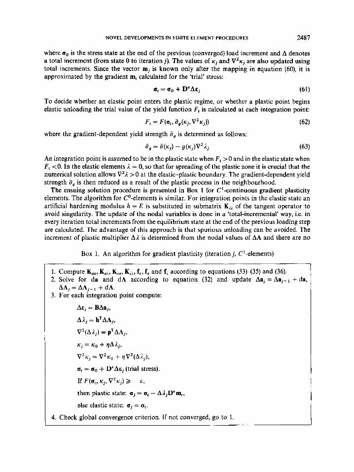
The ensuing solution procedure is presented in Box 1 for C1-continuous gradient plasticity elements. The algorithm for Co-elements is similar. For integration points in the elastic state an artificial hardening modulus h = E is substituted in submatrix KA1 of the tangent operator to avoid singularity. The update of the nodal variables is done in a 'total-incremental' way, i.e. in every iteration total increments from the equilibrium state at the end of the previous loading step are calculated. The advantage of this approach is that spurious unloading can be avoided. The increment of plastic multiplier A l is determined from the nodal values of AA and there are no

Box 1. An algorithm for gradient plasticity (iteration j , C'-elements)

1. Compute K,,, KO,, K,,, KIA, f,, f, and f, according to equations (33H35) and (36). 2. Solve for da and dA according to equation (32) and update Aaj = Aaj-l + da,

3. For each integration point compute: AAj = AAj-1 + dA.

= BAaj,

A I j = bTAAj,

V2(AAj) = pTAAj,

Kj = KO + qAAj,

V2icj = v 2 ~ o + qv2(AAj),

a, = a. + D e A z j (trial stress).

If F(o , , K j , V2ICj) > - E ,

then plastic state: aj = a, - AAjDem,,

else elastic state: aj = at.

4. Check global convergence criterion. If not converged, go to 1.


additional iterations at the integration point level. The updated values of the hardening parameter K~ and its Laplacian VZxj are already available at the trial stress state and are used in the yield condition, but alternatively the memorized values from the previous increment ic0 and V2q, can be used, which results in a slightly delayed plastification. The relation of the present algorithm to the tangent-cutting-plane algorithm18 is not so close as in the ‘delta-incremental’ algorithm in Reference 9.

Because the plastic multiplier is an independent variable determined in the solution of the global set of equations, the weak form of the yield condition (21) is not satisfied until convergence is achieved. It can happen that due to stress redistribution or non-linear softening the increment A 1 results in a return mapping to the inside of the yield surface. In the present total-incremental algorithm this does not cause the detection of unloading, but changes sign of the residual forces, which results further in a proper correction (decrease) of AL. However, difficulties may arise, if the value of the yield function has different signs at the integration points within one element. The respective contributions to residual force f, get averaged because of the weak formulation and improper values of corrections dA are obtained from the global set of equations. Therefore the best convergence is found for those finite elements in which, at the sampling points, the value of the yield function F converges to zero with the decrease of the residual force norm.

The algorithm in Box 1 can also be used for gradient-independent plasticity. However, the introduction of additional nodal degrees of freedom makes it seem inferior to the standard return mapping algorithms. It is noted that for a homogeneous stress state the new formulation can be proved equivalent to the standard plasticity formulation.

6.2. Consistent linearization

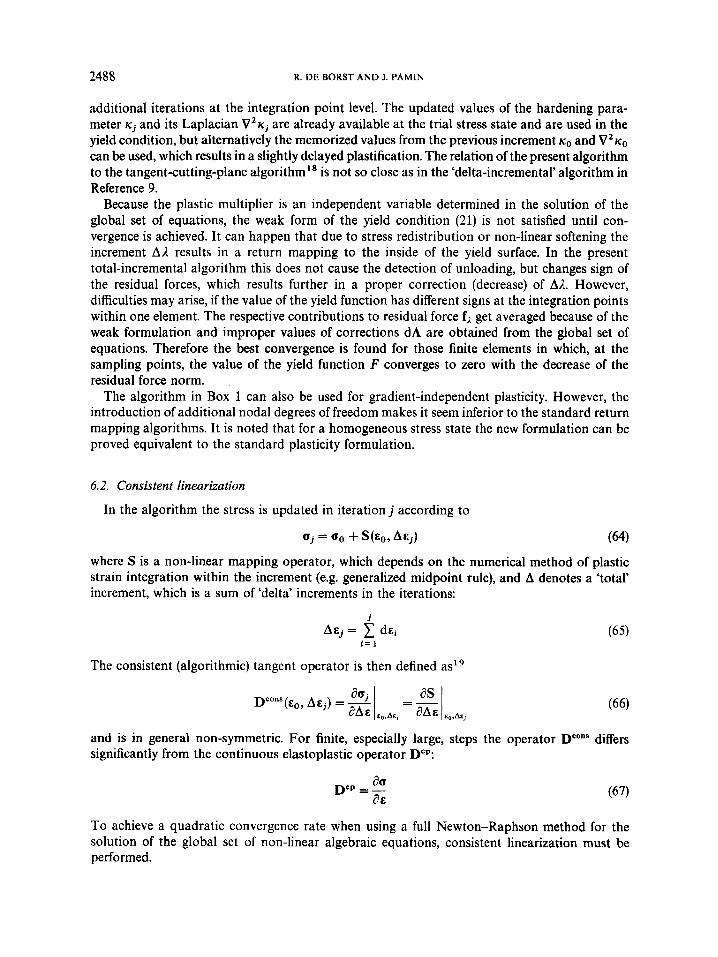
In the algorithm the stress is updated in iteration j according to

where S is a non-linear mapping operator, which depends on the numerical method of plastic strain integration within the increment (e.g. generalized midpoint rule), and A denotes a ‘total’ increment, which is a sum of ‘delta’ increments in the iterations:

j A E ~ = C d&i

i = 1

The consistent (algorithmic) tangent operator is then defined as”

and is in general non-symmetric. For finite, especially large, steps the operator Dcons differs significantly from the continuous elastoplastic operator Dep:

To achieve a quadratic convergence rate when using a full Newton-Raphson method for the solution of the global set of non-linear algebraic equations, consistent linearization must be performed.


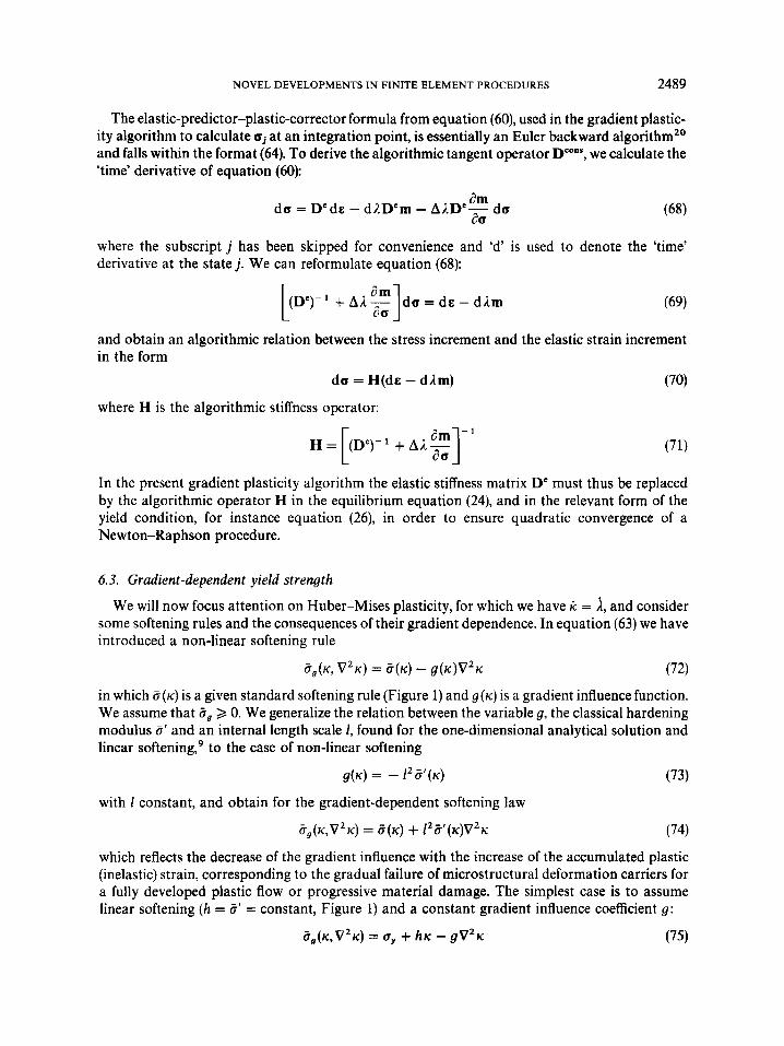
The elastic-predictor-plastic-corrector formula from equation (60), used in the gradient plasticity algorithm to calculate oj at an integration point, is essentially an Euler backward algorithm” and falls within the format (64). To derive the algorithmic tangent operator DCons, we calculate the ‘time’ derivative of equation (60):

dm d a = D”de - dlD‘m - AADe- d a

aa

where the subscript j has been skipped for convenience and ‘d’ is used to denote the ‘time’ derivative at the state j . We can reformulate equation (68):

and obtain an algorithmic relation between the stress increment and the elastic strain increment in the form

d o = H(de - d h ) (70)

where H is the algorithmic stiffness operator:

In the present gradient plasticity algorithm the elastic stiffness matrix D’ must thus be replaced by the algorithmic operator H in the equilibrium equation (24), and in the relevant form of the yield condition, for instance equation (26), in order to ensure quadratic convergence of a Newton-Raphson procedure.

6.3. Gradient-dependent yield strength

We will now focus attention on Huber-Mises plasticity, for which we have ic = A, and consider some softening rules and the consequences of their gradient dependence. In equation (63) we have introduced a non-linear softening rule

( r s ( K , v2K) = C ( K ) - g ( K ) v z K (72)

in which d ( ~ ) is a given standard softening rule (Figure 1) and g ( K ) is a gradient influence function. We assume that Cg 2 0. We generalize the relation between the variable g, the classical hardening modulus 0’ and an internal length scale 1, found for the one-dimensional analytical solution and linear softening,’ to the case of non-linear softening

g ( K ) = - l 2 8 ’ ( K ) (73)

with 1 constant, and obtain for the gradient-dependent softening law

(r,(K,V2K) = C(K) + IZi?’(K)V2K (74)

which reflects the decrease of the gradient influence with the increase of the accumulated plastic (inelastic) strain, corresponding to the gradual failure of microstructural deformation carriers for a fully developed plastic flow or progressive material damage. The simplest case is to assume linear softening (h = 5’ = constant, Figure 1) and a constant gradient influence coefficient g :

c g ( ~ , V 2 ~ ) = oy + h K - gVZK (75)


The gradient-dependent yield strength in equation (72) is composed of two contributions. The gradient contribution -g(K)V2rc may be positive or negative as shown in Figure 2. The former case occurs in the middle of the localization band, giving additional carrying capacity to the gradient-dependent material in this area: even if 5 equals zero, the yield strength 5, is larger than zero. The case of negative gradient contribution occurs at the elastic-plastic boundary, making it possible for the localization zone to spread, since the elastic elements close to the elastic-plastic boundary have an apparent reduced yield strength. These modifications of the standard yield strength ~ ( I c ) are the algorithmic essence of the gradient regularization.

We consider now the problem of a vanishing yield strength. When the local residual strength is exhausted in standard softening plasticity, i.e. when the yield surface has shrunk to zero @(K) -, 0), further calculations should still be possible under displacement control. However, in this limiting case the yield function becomes singular and the tangent operator may become ill-conditioned. To prevent this a small positive number can be introduced instead of zero as the limit value of the yield strength 5 ( ~ , ) , cf. Figure 1.

The problem is more delicate in gradient plasticity. As shown in Figure 2, the limit case 5, + 0 can be reached at a state, for which 5 > O (IC <xu). This happens easily for linear softening and less

Figure 1. Linear and non-linear softening diagrams

Figure 2. Gradient contribution to the yield strength

NOVEL DEVELOPMENTS IN FINITE ELEMENT PROCEDURES 249 1

quickly for non-linear softening functions as in Figure 1, since the gradient contribution in equation (74) goes to zero together with if@). To prevent the occurrence of numerical difficulties when the yield strength reaches zero as well as the unacceptable situation of a negative Cq, its value is bounded by a small positive number (e.g. 5, > and a corrective procedure is suggested to avoid a spurious return mapping to stress states of the opposite sign. The procedure resolves in one additional (global) iteration the case of return mapping to the other side or to the inside of the shrinking yield surface (cf. Figure 2). From the numerical viewpoint, for non-linear softening both limits aq -, 0 and g --* 0 should be avoided. Therefore non-linear softening to zero is not allowed and the values of 6 and g for K = 0.98 K , are kept constant for K > 0.98~". From the physical viewpoint, the element topology should be modified at this stage by introducing interface elements modelling a discrete displacement discontinuity.

7. SOME ELEMENTS FOR GRADIENT PLASTICITY

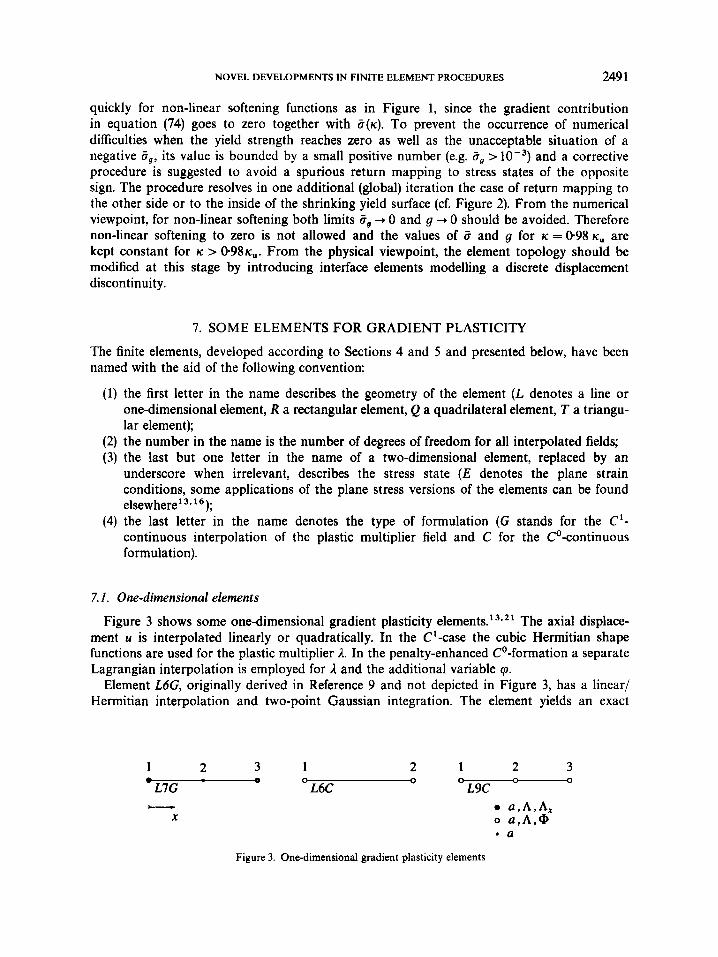
The finite elements, developed according to Sections 4 and 5 and presented below, have been named with the aid of the following convention:

(1) the first letter in the name describes the geometry of the element ( L denotes a line or one-dimensional element, R a rectangular element, Q a quadrilateral element, T a triangular element);

(2) the number in the name is the number of degrees of freedom for all interpolated fields; (3) the last but one letter in the name of a two-dimensional element, replaced by an

underscore when irrelevant, describes the stress state (E denotes the plane strain conditions, some applications of the plane stress versions of the elements can be found elsewhere' 3* ' );

(4) the last letter in the name denotes the type of formulation (G stands for the C'- continuous interpolation of the plastic multiplier field and C for the Co-continuous formulation).

7.1. One-dimensional elements

Figure 3 shows some one-dimensional gradient plasticity elements.' 3*2 The axial displacement u is interpolated linearly or quadratically. In the Cl-case the cubic Hermitian shape functions are used for the plastic multiplier 1. In the penalty-enhanced Co-formation a separate Lagrangian interpolation is employed for 1 and the additional variable cp.

Element L6G, originally derived in Reference 9 and not depicted in Figure 3, has a linear/ Hermitian interpolation and two-point Gaussian integration. The element yields an exact

1 2 3 1 2 1 2 3

' L7G L6C 0 0 0 -

OL9C - 0 - X

Figure 3. One-dimensional gradient plasticity elements


fulfilment of the yield condition at the integration points, which means that when f, --+ 0, then F j = F ( G ~ , K ~ , V ~ K ~ ) + 0, but stress oscillations are observed. This phenomenon may cause a failure of convergence at an early stage of softening as soon as the oscillating stresses reach a state with Cq + 0.

For element L7G, which has a quadratic/Hermitian interpolation (cf. Figure 3) and two- point integration, the balance between the interpolation for u and ;1 is optimal, i.e. the stress integration in equation (60) gives a stress state oj , which is constant within an element and which fulfils exactly the yield condition. Convergence in one iteration is observed unless the softening zone spreads or non-linear softening is used. This behaviour is attributed to the special qualities of the integration stations, so-called Barlow points,22 in which higher-order accuracy of interpolated field derivatives is obtained. In fact, these are the only points in which the third-order terms in F (aj, l c j , V2xj) cancel the first-order terms, so that the yield function equals zero.

The above properties are exhibited by the non-symmetric formulation with KAA from equation (35). If the symmetric format for KLA according to equation (37) is used together with the required boundary conditions and two-point (reduced) integration, convergence is lost. This behaviour is attributed to a numerical integration error, since for three-point integration the symmetric and non-symmetric formulations give the same results. However, for the three-point integration too many constraints are introduced and the results are inaccurate. The stresses at one or more points are then mapped to the inside of the yield surface ( F j cO), which violates the Kuhn-Tucker conditions (6) and results in a disturbance of convergence.

The Co-continuous element L6C uses linear shape function for all the unknowns and one integration point. It is the point in which the constraint cp = I , , is fulfilled. The element is perfectly convergent since the integration station is a Barlow point.22 Element L9C uses quadratic shape functions and two Gauss points, which are again optimal for convergence and therefore the return mapping is exact. In the presence of the additional boundary conditions (59) the symmetric and non-symmetric formulations give the same results for the one-dimensional penalty-enhanced elements, because the employed numerical integration schemes are sufficient for an exact integration of the shape function polynomials.

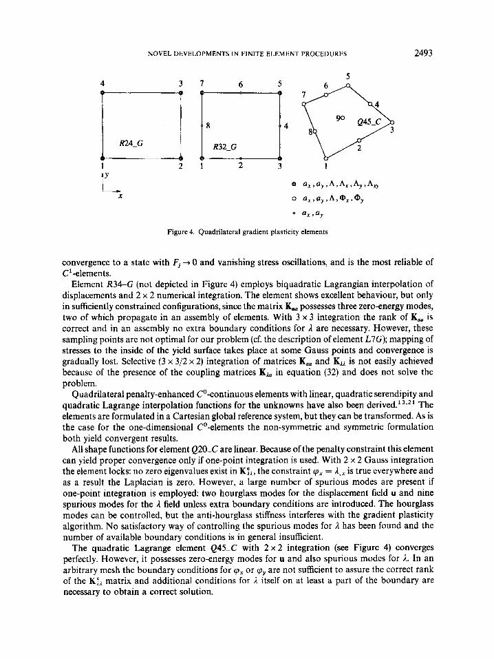
7.2. Quadrilateral elements

Figure 4 shows some of the possible quadrilateral gradient plasticity elements.' 3 7 2 1 The C'-continuous rectangles have a varying interpolation of the displacements and the same bi-Hermitian shape functions for the plastic multiplier field. The elements are formulated in a Cartesian global reference system and cannot be transformed because of the presence of the mixed derivative degrees of freedom Axy in the C'4nterpolation of I . Only the non-symmetric formulation of the problem yields in this case fully convergent results.

Element R24-G employs a bilinear interpolation of the displacements and selective integration. Matrix K,, possesses the correct rank, but the matrix KZL requires 12 additional constraints, which can be introduced by extra boundary conditions for derivatives of A. For an arbitrary assembly the conditions An = 0 and Axy = 0 on the whole model boundary supply exactly the required number of constraints. Element R24-G gives Fj -+ 0 at the integration point, but as the one-dimensional element L6G it shows stress oscillations due to the lack of balance between the employed interpolations.

Element R32-G employs eight-noded serendipity interpolation of displacements and 2 x 2 Gauss integration. The matrix K,, possesses one zero-energy mode that disappears in an assembly of elements. With the matrix K; described above, this element shows proper


4 3

1 2

L X

Figure 4. Quadrilateral gradient plasticity elements

convergence to a state with Fj + 0 and vanishing stress oscillations, and is the most reliable of C'-elements.

Element R34-G (not depicted in Figure 4) employs biquadratic Lagrangian interpolation of displacements and 2 x 2 numerical integration. The element shows excellent behaviour, but only in sufficiently constrained configurations, since the matrix K,, possesses three zero-energy modes, two of which propagate in an assembly of elements. With 3 x 3 integration the rank of K,, is correct and in an assembly no extra boundary conditions for 1 are necessary. However, these sampling points are not optimal for our problem (cf. the description of element L7G); mapping of stresses to the inside of the yield surface takes place at some Gauss points and convergence is gradually lost. Selective (3 x 3/2 x 2) integration of matrices K,, and K I A is not easily achieved because of the presence of the coupling matrices KI, in equation (32) and does not solve the problem.

Quadrilateral penalty-enhanced Co-continuous elements with linear, quadratic serendipity and quadratic Lagrange interpolation functions for the unknowns have also been derived.' 3*21 The elements are formulated in a Cartesian global reference system, but they can be transformed. As is the case for the one-dimensional Co-elements the non-symmetric and symmetric formulation both yield convergent results.

All shape functions for element Q20-C are linear. Because of the penalty constraint this element can yield proper convergence only if one-point integration is used. With 2 x 2 Gauss integration the element locks: no zero eigenvalues exist in K:l, the constraint cpx = is true everywhere and as a result the Laplacian is zero. However, a large number of spurious modes are present if one-point integration is employed: two hourglass modes for the displacement field u and nine spurious modes for the I field unless extra boundary conditions are introduced. The hourglass modes can be controlled, but the anti-hourglass stiffness interferes with the gradient plasticity algorithm. No satisfactory way of controlling the spurious modes for il has been found and the number of available boundary conditions is in general insufficient.

The quadratic Lagrange element Q45-C with 2 x 2 integration (see Figure 4) converges perfectly. However, it possesses zero-energy modes for u and also spurious modes for 1. In an arbitrary mesh the boundary conditions for cpx or cpy are not sufficient to assure the correct rank of the K:). matrix and additional conditions for I I itself on at least a part of the boundary are necessary to obtain a correct solution.


The quadratic serendipity element Q40-C with 2 x 2 integration does not converge very well, since the return mapping in equation (60) is inaccurate for this element. Apparently the quadratic terms missing in the serendipity interpolation are important for interpolation compatibility. Since an assembly of elements Q40-C does not possess hourglass deformation modes, a combination of eight-noded interpolation of displacements and nine-noded interpolation of the I and 4 fields is suggested and gives rise to element Q43-C, quite similar to the' 'heterosis' plate bending elements.23 This element converges better and is a Co-equivalent of the eight-noded element R32G.

7.3. Triangular elements

For a triangular element geometry the problem of choosing well-balanced interpolations of displacements and plastic multiplier as well as optimal integration scheme becomes even more d i f f i~ul t . '~*~ ' Experience with rectangles suggests the use of the lowest possible interpolation order and reduced integration. Figure 5 shows three triangular elements, which have a quadratic interpolation of displacements. The elements are formulated in area co-ordinates and, to avoid transformations, are referred to the global axes.

Element T21-G has a cubic interpolation of 1 based on a non-conforming plate bending triangle.z3 The element does not fulfill the continuity requirements for I,, on its boundary and is included in the group of C'-elements because of the presence of A, and A, degrees of freedom. Integration with three Gauss points or three Hammer points (at the midsides of the triangle) is applied. Neither of these integration schemes is optimal: stresses are mapped inside the yield surface and stress oscillations are found. Additional boundary conditions for the plastic multiplier field are necessary to prevent the existence of non-zero A modes in the elastic elements.

Element T30-G employs the shape functions derived in Reference 24, has a quintic interpolation of A and cubic distribution of A,, along the sides and is fully C'-compatible. To prevent spurious 1 modes six integration points and extra boundary conditions, involving A,, or A, and sometimes also second-order derivatives of the plastic multiplier are necessary.

It seems that for the above elements it is not possible to find sampling points in which higher-order accuracy of stress approximation and convergence of Fj to zero is obtained. Consequently neither of them exhibits a fast convergence and stress oscillations are observed that may lead to violation of the positive yield strength condition and sometimes also to local

1

L X

1

Figure 5. Triangular gradient plasticity elements


unloading. Nevertheless, in numerical tests with Huber-Mises gradient plasticity they give reasonable predictions of the global response and shear banding.

It is also difficult to construct Co-continuous triangular elements which satisfy the requirements for interpolation and numerical integration. We have limited our research to a low-order interpolation and have obtained only one applicable element.'3*21 This element, called T30-C, has a uniform quadratic interpolation and is integrated using three Gauss points. Although full convergence is not achieved-mapping of stresses to the inside of the yield surface is observed and stress oscillations are found-this element gives acceptable results. In constrained configurations the use of one-point integration yields fast convergence and three integration points may cause locking.

8. THE REGULARIZING EFFECT OF GRADIENT PLASTICITY

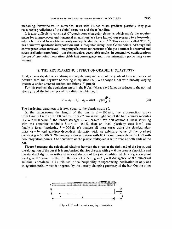
First, we investigate the stabilizing and regularizing influence of the gradient term in the case of positive, zero and negative hardening in equation (72). We analyse a bar with linearly varying thickness under uniaxial tension conditions (Figure 6).

For this problem the equivalent stress in the Huber-Mises yield function reduces to the normal stress ox and the following yield condition is obtained:

The hardening parameter IC is now equal to the plastic strain 6;. In the calculations the length of the bar is L = 100 mm, the cross-section grows

from 1 mm x 1 mm at the left end to 1 mm x 2 mm at the right end of the bar, Young's modulus is E = 20000 N/mm2, the tensile strength oy = 2 N/mm2. We first assume a linear softening with the softening modulus h = 8' = - 0.1 E, then an ideal plasticity case h = 0 and finally a linear hardening h = 005 E. We analyse all these cases using the classical plasticity (g = 0) and gradient-dependent plasticity with an arbitrary value of the gradient constant g = 50000 N. We employ a discretization with 80 C'-continuous elements L7G with two integration points. The derivative of the plastic multiplier is set to zero at both ends of the bar.

Figure 7 presents the calculated relations between the stress at the right end of the bar o, and the elongation of the bar U. It is emphasized that for the case with g = 0 the present algorithm and the standard algorithm with a strong satisfaction of the yield condition at the integration point level give the same results. For the case of softening and g = 0 divergence of the numerical solution is obtained. It is attributed to the incapability of reproducing localization in only one integration point, which is triggered by the linearly changing geometry of the bar. On the other

4

T I ' X

I- L P -

I c

Figure 6. Tensile bar with varying cross-section


hand the calculations for g = 50000 N converge perfectly and produce the expected smooth distribution of the plastic strains as shown in the right part of Figure 7. We observe that the localization zone first grows from the thinnest elements, then its width is almost constant while the solution follows the linear softening branch and finally, when U > 1.05 x mm, the plastic zone starts to grow again while the load-displacement diagram bends upwards. This effect will be further discussed in the next section.

The diagrams for ideal and hardening plasticity (Figure 7) demonstrate the stabilizing influence of the gradient term with g > O . Figures 8 and 9 compare distributions of plastic strains calculated in the analysed loading history for the classical and gradient-dependent case. In the classical ideal plasticity problem the strains are confined in a small zone at the weakest cross-section, which corresponds to the limiting case of the loss of material stability and ellipticity. The gradient term introduces an apparent hardening and produces a gradual expansion of the plastic zone (note that the strain scale is different in the two diagrams of Figure 8). In the hardening plasticity cases we

ur [Nlmm2] x~o-’ A

1.4

1.2

1

0.8

0.6

0.4

0.2

0

-gradient plasticity ---classical plasticify

6 O h 3 0.06 0.609 O.dl2 O h 5

1.5

1.2

0.9

0.6

0.3

0

ii [mm] x - coordinate [mm]

Figure 7. Load-displacement diagrams for softening/ideal/hardening plasticity (classical and gradient-dependent case) and localization of plastic strains at the smallest cross-section

XIO-~ A 10

8

6

4

2

0

X IO-~ A

I I 1.0

1 30 1 40

10.6

1 0 50

x - coordinate [mm] x - coordinate [mm]

Figure 8. Localization of plastic strains for classical ideal plasticity and evolution of plastic strains for gradient plasticity with zero hardening


x~o-' A x ~ o - ~ A


Figure 9. Evolution of the plastic front in classical and gradient-dependent hardening plasticity

observe the expected motion of the plastic front, but with g = 50000 N the expansion of the plastic zone is faster and the strain profiles are smooth (regularized).

9. LOCALIZATION ANALYSES USING GRADIENT PLASTICITY

9. I . One-dimensional elements

We analyse a similar bar in tension,' but now with a constant thickness (unit cross-section) and an imperfection as shown in Figure 10. The elements in the centre of the bar (d = 10 mm) have a 10 per cent smaller value of the tensile strength cry. The following data are as before: L = 100 mm, E = 20000 N/mm2, cry = 2 N/mmz. Two meshes with 20 and 80 one-dimensional gradient plasticity elements are used to examine the mesh sensitivity of results.

According to the analytical s ~ l u t i o n ~ . ' ~ for the case of linear softening the width of the localization zone, w, is related to the constant g via the internal length 1 and the hardening (softening) modulus h = 0':

w = 2x1, 1 = J--y/h (77)

First the case of linear softening is analysed with the softening modulus h = - 0.1E. The internal length 1 = 5 mm is assumed, which gives according to equation (77) the gradient constant g = - 12h = 50 000 N and the width of the localization zone w = 31.4 mm. We begin the comparison with Co-continuous penalty-enhanced elements. The left diagram in Figure 1 1 shows load-displacement paths obtained using elements L6C and L9C with the (optimal) one-point and two-point Gauss integration, respectively. In the same figure on the right stress-strain relations exhibited by different elements in the 20-element mesh are shown (element 10 lies at the symmetry axis, element 9 to the left etc.). As can be seen for elements 8 and 7, the yield strength is correctly reduced owing to the evolving plastic process in the adjacent elements (non-local behaviour). It is also stressed that in the absence of a localization limiter only the weaker element 10 would follow the softening path and the other elements would unload.

Immediate convergence has been observed in the calculations. While the coarse mesh with 20 linear elements L6C still gives slightly too stiff response and a disturbed L distribution (Figure 12),

2498

1.6 -

1.2 -

0.8 -

0.4 -

R. DE BORST AND J. PAMIN

O V

X . u r- I

Figure 10. Imperfect bar in pure tension

u [Nlmm2] 2.0 , I

u [Nlmm2] r2.0

----Average ---Elem. 10 ---Elem. 9 -Elem. 8

' \ \. \. -Elem. 7 \\ \-

-1.6

1.2

- L . 4

14 0!3 016 0:9 112 1:s 1:s

XIO-~ E

Figure 11. Load4isplacement diagrams for one-dimensional C'elements (left) and stress-strain paths followed by different elements in the middle of the bar discretized with 20 linear elements L6C (right)

x10-3 A x10-3 A 1.5 I I /

1.2

0.9

0.6

0.3

0 io 40 do 80 Id0 b do do do so 1

I 1

1.5

1.2

0.9

0.6

0.3

0

O x - coordinate [mm] x -coordinate [mm]

Figure 12. Evolution of the plastic strain distribution in the bar for 20 (left) and 80 (right) elements L6C

the fine mesh and both meshes for the quadratic L9C element yield identical results. It is observed that when all the plastic points in the structure are in the softening regime, the slope of the load-displacement diagram is equal to the analytical ~ a l u e ~ . ' ~ and the width of the localization band is set by the internal length 1. The calculations are stable when the strain in the centre elements exits the softening branch (IC > K"). The load-displacement diagrams then bend upwards


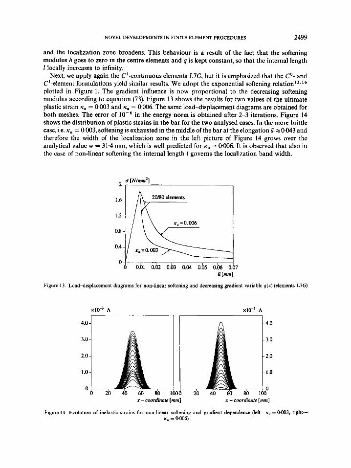
and the localization zone broadens. This behaviour is a result of the fact that the softening modulus h goes to zero in the centre elements and g is kept constant, so that the internal length I locally increases to infinity.

Next, we apply again the C1-continuous elements L7G, but it is emphasized that the Co- and C'-element formulations yield similar results. We adopt the exponential softening r e l a t i ~ n ' ~ . ' ~ plotted in Figure 1. The gradient influence is now proportional to the decreasing softening modulus according to equation (73). Figure 13 shows the results for two values of the ultimate plastic strain K , = 0.003 and K , = 0.006. The same load-displacement diagrams are obtained for both meshes. The error of in the energy norm is obtained after 2-3 iterations. Figure 14 shows the distribution of plastic strains in the bar for the two analysed cases. In the more brittle case, i.e. K , = 0.003, softening is exhausted in the middle of the bar at the elongation U ~ 0 . 0 4 3 and therefore the width of the localization zone in the left picture of Figure 14 grows over the analytical value w = 31.4 mm, which is well predicted for K, = 0.006. It is observed that also in the case of non-linear softening the internal length 1 governs the localization band width.

-

0 O h 1 0.b 0.03 0 . b 0.05 0.h 0.07 : [MI

Figure 13. Load4isplacement diagrams for non-linear softening and decreasing gradient variable g(K) (elements L7G)

x ~ o - ~ A x ~ o - ~ A

4.0

3.0

2.0

1 .o

0


Figure 14. Evolution of inelastic strains for non-linear softening and gradient dependence (left-ic. = O G I 3 , right- K, = 0.006)


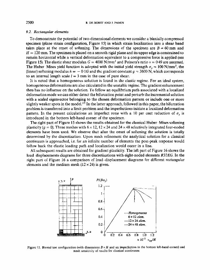
9.2. Rectangular elements

To demonstrate the potential of two-dimensional elements we consider a biaxially compressed specimen (plane strain configuration, Figure 15) in which strain localization into a shear band takes place at the onset of softening. The dimensions of the specimen are B = 60 mm and H = 120 mm. The specimen is placed on a smooth rigid plane and its upper edge is constrained to remain horizontal while a vertical deformation equivalent to a compressive force is applied (see Figure 15). The elastic shear modulus G = 4000 N/mm2 and Poisson’s ratio v = 0.49 are assumed. The Hube-Mises yield function is adopted with the initial yield strength cy = 100 N/mm2, the (linear) softening modulus h = - 0.1G and the gradient constant g = 3600 N, which corresponds to an internal length scale 1 = 3 mm in the case of pure shear.

It is noted that a homogeneous solution is found in the elastic regime. For an ideal system, homogeneous deformations are also calculated in the unstable regime. The gradient enhancement then has no influence on the solution. To follow an equilibrium path associated with a localized deformation mode we can either detect the bifurcation point and perturb the incremental solution with a scaled eigenvector belonging to the chosen deformation pattern or include one or more slightly weaker spots in the In the latter approach, followed in this paper, the bifurcation problem is transferred into a limit problem and the imperfections initiate a localized deformation pattern. In the present calculations an imperfect zone with a 10 per cent reduction of (T,, is introduced in the bottom left-hand corner of the specimen.

The right part of Figure 15 shows the results obtained for the classical Huber-Mises softening plasticity (g = 0). Three meshes with 6 x 12, 12 x 24 and 24 x 48 selectively integrated four-noded elements have been used. We observe that after the onset of softening the solution is totally determined by the discretization. Upon mesh refinement the analytical solution for a classical continuum is approached, i.e. for an infinite number of elements the post-peak response would follow back the elastic loading path and localization would occur in a line.

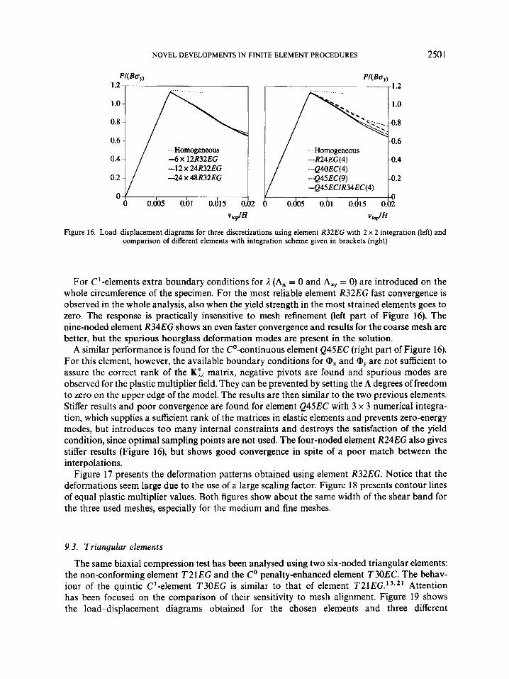
All subsequent results are obtained for gradient plasticity. The left part of Figure 16 shows the loadclisplacements diagrams for three discretizations with eight-noded elements R32EG. In the right part of Figure 16 a comparison of load-displacement diagrams for different rectangular elements and the medium mesh (12 x 24) is given.

W B U J

1.2

----Homogeneous 4 x 12 elem. -1 2 x 24 elem. -24 x 48 elem.

0 0.2 0.4 0.6 0.8 1.0 1.2 x V , ~ , / H

Figure 15. Biaxial test configuration (with dimensions B x H and an imperfection in the bottom left-hand corner) and mesh sensitivity of results for classical continuum


0.8

0.6 -.Homogeneous

-Q45ECIR34EC(4)

0.005 0.01 0.015 0.02 v*0plH

Figure 16. Load4isplacement diagrams for three discretizations using element R32EG with 2 x 2 integration (left) and comparison of different elements with integration scheme given in brackets (right)

For C1-elements extra boundary conditions for 1 (A,, = 0 and Axy = 0) are introduced on the whole circumference of the specimen. For the most reliable element R32EG fast convergence is observed in the whole analysis, also when the yield strength in the most strained elements goes to zero. The response is practically insensitive to mesh refinement (left part of Figure 16). The nine-noded element R34EG shows an even faster convergence and results for the coarse mesh are better, but the spurious hourglass deformation modes are present in the solution.

A similar performance is found for the Co-continuous element Q45EC (right part of Figure 16). For this element, however, the available boundary conditions for Ox and Oy are not sufficient to assure the correct rank of the K:A matrix, negative pivots are found and spurious modes are observed for the plastic multiplier field. They can be prevented by setting the A degrees of freedom to zero on the upper edge of the model. The results are then similar to the two previous elements. Stiffer results and poor convergence are found for element Q45EC with 3 x 3 numerical integration, which supplies a sufficient rank of the matrices in elastic elements and prevents zero-energy modes, but introduces too many internal constraints and destroys the satisfaction of the yield condition, since optimal sampling points are not used. The four-noded element R24EG also gives stiffer results (Figure 16), but shows good convergence in spite of a poor match between the interpolations.

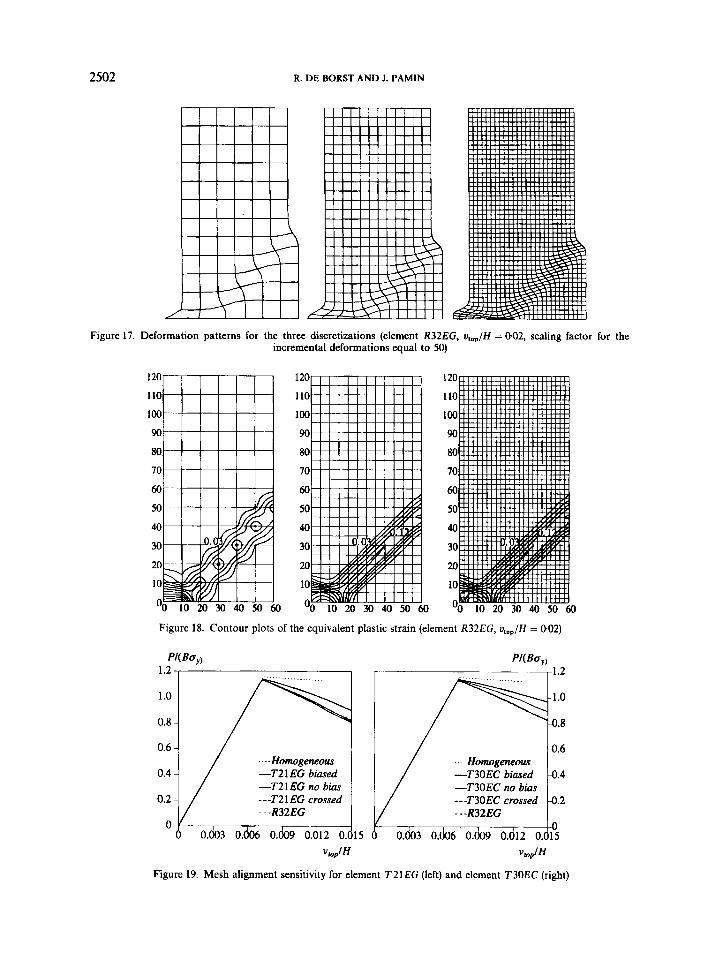
Figure 17 presents the deformation patterns obtained using element R32EG. Notice that the deformations seem large due to the use of a large scaling factor. Figure 18 presents contour lines of equal plastic multiplier values. Both figures show about the same width of the shear band for the three used meshes, especially for the medium and fine meshes.

9.3. Triangular elements

The same biaxial compression test has been analysed using two six-noded triangular elements: the non-conforming element T21 EG and the Co penalty-enhanced element T30EC. The behaviour of the quintic C'-element T30EG is similar to that of element T21EG.13**' Attention has been focused on the comparison of their sensitivity to mesh alignment. Figure 19 shows the load-displacement diagrams obtained for the chosen elements and three different


Figure 17. Deformation patterns for the three discretizations (element R32EG, u,.,/H = 002, scaling factor for the incremental deformations equal to 50)

120

110

100

90

80

70

60

50

40

30

20

10

OO LO 20 30 40 50 60

120

110

100

90

80

I0

60

50

40

30

20

10

'0 10 20 30 40 50 60

Figure 18. Contour plots of the equivalent plastic strain (element R32EG, u,&f = 0.02)

1.2

1 .o

0.8

0.6

0.4

0.2

0

- - - -Homogeneous -T21 EG biased -T21 EG no bias ---T21 EG crossed

; - -RTEG 1 0.003 0. 0.009 0. 12 0. 15

vmJH

Homogeneous -T30EC biased -T30EC no bias ---T30EC crossed - - -R32EG

.6

.4

.2

10 O h 3 O h 6 0 . b O.dl2 O.dl5

VtOplH

Figure 19. Mesh alignment sensitivity for element T 2 l E G (left) and element T30EC (right)


discretizations: 12 x 24 x 4 (crossed-diagonal), 12 x 24 x 2 with the element lines parallel to the expected direction of the shear band and 12 x 24 x 2 with the elements aligned perpendicularly to the shear band.

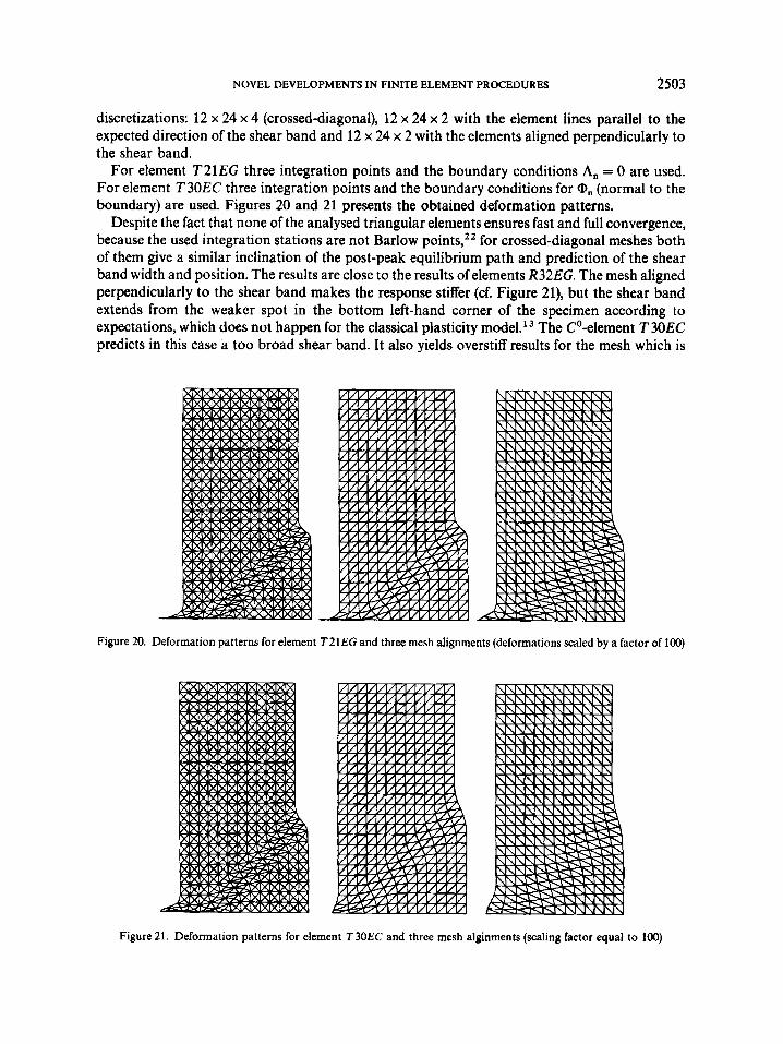
For element T21EG three integration points and the boundary conditions A,, = 0 are used. For element T30EC three integration points and the boundary conditions for Q,, (normal to the boundary) are used. Figures 20 and 21 presents the obtained deformation patterns.

Despite the fact that none of the analysed triangular elements ensures fast and full convergence, because the used integration stations are not Barlow points:' for crossed-diagonal meshes both of them give a similar inclination of the post-peak equilibrium path and prediction of the shear band width and position. The results are close to the results of elements R32EG. The mesh aligned perpendicularly to the shear band makes the response stiffer (cf. Figure 21), but the shear band extends from the weaker spot in the bottom left-hand corner of the specimen according to expectations, which does not happen for the classical plasticity m0de1.I~ The Co-element T 30EC predicts in this case a too broad shear band. It also yields overstiff results for the mesh which is

Figure 20. Deformation patterns for element T2lEG and three mesh alignments (deformations scaled by a factor of 100)

Figure 21. Deformation patterns for element T30EC and three mesh alginments (scaling factor equal to 100)


aligned parallel to the shear band direction. The results for element T21EG are better and the slight mesh alignment sensitivity is expected to vanish upon a further mesh refinement.

10. CONCLUDING REMARKS

In this paper various aspects of finite element implementation of gradient-dependent plasticity have been studied. The theory includes a regularizing dependence of the yield function on the Laplacian of a plastic strain measure. The fundamental feature of the used algorithm is the weak (and not pointwise) satisfaction of the yield condition, which is coupled with the weak equilibrium condition.

A new, Co-continuous formulation has been developed, in which the continuity requirements are relaxed by treating the first derivatives of the plastic multiplier as additional unknowns and connecting them to the plastic multiplier field using a penalty constraint. Several C'- and Co-continuous, one-dimensional, rectangular and triangular elements have been examined. The consistent tangent operator has been derived and the algorithmic consequences of the gradient dependence of the yield strength have been investigated.

The implemented elements introduce properly the stabilizing and regularizing properties of the gradient-dependent continuum. The results of finite element simulations are almost insensitive to mesh refinement and alignment, since the width of the shear bands is determined by the internal length scale included in the theory. However, it is emphasized that for robustness the elements should fulfill some additional conditions:

(a) The balance of interpolations for displacements u and plastic multiplier A. The best agreement is found between quadratic shape functions for u and cubic Hermitian polynomials for A or quadratic shape functions for A and its derivatives.

(b) The existence of a suitable integration quadrature. A proper number of integration points is necessary to prevent zero-energy modes for u and A fields without introducing too many constraints. The sampling positions should be optimal for accuracy.

(c) The availability of additional boundary conditions for the A field, necessary in combination with a symmetric tangent operator and helpful in removing spurious modes for the plastic multiplier field.

Failure to satisfy these conditions manifests itself by stress oscillations and/or incorrect return mappings, deteriorating the convergence rate and reliability of the solution. Since the employed set of integral equations for equilibrium and plastic yielding is coupled, an error in the satisfaction of one equation may affect adversely the other equation.

Among the analysed two-dimensional elements only the eight-noded serendipity/Hermitian element R32-G fulfils all the requirements, but the nine-noded elements R34-G and Q45-C/Q43-C also give proper results if a sufficient number of additional boundary constraints are introduced in the model. Among the implemented triangular elements the six-noded quadratic/non-conforming element T21-G with three integration points performs the best.

ACKNOWLEDGEMENTS

The calculations have been carried out with a pilot version of the DIANA finite element code of TNO Building and Construction Research. The financial support of the Commission of the European Communities through the Brite-Euram program (project BE-3275) and the fruitful discussions with Dr.-Ing. H.-B. Muhlhaus (CSIRO Division of Exploration and Mining) are gratefully acknowledged.


REFERENCES

1. R. de Borst, L. J. Sluys, H.-B. Miihlhaus and J. Pamin, ‘Fundamental issues in finite element analyses of localization of

2. K. J. Willam and A. Dietsche, ‘Fundamental aspects of strain-softening descriptions’, in Z. P. Baiant (ed.), Fracture

3. L. J. Sluys, ‘Wave propagation, localization and dispersion in softening solids’, Dissertation, Delft University of

4. E. C. Aifantis, ‘On the microstructural origin of certain inelastic models’, J. Eng. Mater. Techno/., 106,326-330(1984). 5. E. C. Aifantis, ‘The physics of plastic deformation’, Int. J . Plasticiry, 3, 211-247 (1987). 6. H. M. Zbib and E. C. Aifantis, ‘On the localization and postlocalization behavior of plastic deformation, I,lI,llI’, Res.

7. H.-B. Miihlhaus and E. C. Aifantis, ‘A variational principle for gradient plasticity’, Int. J. Solids Struct., 28,845-857

8. I. Vardoulakis and E. C. Aifantis, ‘A gradient flow theory of plasticity for granular materials’, Acta Mechanica, 87,

9. R. de Borst and H.-B. Miihlhaus, ‘Gradient-dependent plasticity: formulation and algorithmic aspects’, Int. j. numer.

10. E. C. Aifantis, ‘On the role of gradients in the localization of deformation and fracture’, Int. J. Eng. Sci., 30, 1279-1299

11. Z. P. Baiant and F.-B. Lin, “on-local yield limit degradation’, Int. j. numer. methods eng., 26, 1805-1823 (1988). 12. G. Pijaudier-Cabot and A. Huerta, ‘Discretization influence on regularization by two localization limiters’, J. Eng.

Mech. Diu. ASCE, 1198-1218 (1994). 13. J. Pamin. ‘Gradient-dependent plasticity in numerical simulation of localization phenomena’, Dissertation, Delft

University of Technology, Delft, 1994. 14. L. J. Sluys, R. de Borst and H.-B. Muhlhaus, ‘Wave propagation, localization and dispersion in a gradient-dependent

medium’, Int. J. Solids Struct., 30, 1153-1171 (1993). 15. 0. C. Zienkiewicz and S. Nakazawa, ‘The penalty function and its applications to the numerical solution of boundary

value problems’, Am. Soc. Mech. Eng. AMD, 51, 157-179 (1982). 16. J. Pamin and R. de Borst, ‘Gradient plasticity and finite elements in the simulation of concrete fracture’ in H. Mang

et a!. (eds.), Proc. EURO-C 1994 Int. Con& Computer Modelling of Concrete Structures, Pineridge Press, Swansea, 1994, pp. 393402.

17. M. Ortiz and G. R. Morris, ‘Co finite element discretization of Kirchhoff‘s equations of thin plate bending’, Int. j . numer methods eng., 26, 1551-1566 (1988).

18. M. Ortiz and J. C. Simo, ‘An analysis of a new class of integration algorithms for elastoplastic constitutive relations’, Int. j. numer. methods eng., 23, 353-366 (1986).

19. J. C. Simo and R. L. Taylor, ‘Consistent tangent operators for rate-independent elastoplasticity’, Comput. Methods Appl. Mech. Eng., 48, 101-118 (1985).

20. M. A. Crisfield, Non-Linear Finite Element Analysis ojsol ids and Structures, Vol. I, Chapter 6, Wiley, Chichester, 1991.

21. R. de Borst, J. Pamin and L. J. Sluys, ‘Computational issues in gradient plasticity’, in H.-B. Miihlhaus (ed.), Continuum Modelsfor Materials with Micro-Structure, Chapter 6, Wiley, Chichester, 1995.

22. J. Barlow, ‘Optimal stress locations in finite element model’, Int. j . numer. methods eng., 10, 243-251 (1976). 23. 0. C. Zienkiewicz and R. L. Taylor, The Finite Element Method, Vol. 2, Chapterl, 4th edn, McGraw-Hill, London,

24. S. Dasgupta and D. Sengupta, ‘A higher-order triangular plate bending element revisited‘, I n [ . j . numer. methods eng.,

25. R. de Borst, ‘Numerical methods for bifurcation analysis in geomechanics’, 1ng.-Arch., 59, 16C174 (1989).

deformation’, Eng. Comput., 10, 99-121 (1993).

Mechanics of Concrete Structures, Elsevier Applied Science, London, 1992, pp. 227-230.

Technology, Delft, 1992.

Mechanica, 23, 261-277,279-292,293-305 (1988).

(1991).

197-217 (1991).

methods eng., 35, 521-539 (1992).

(1992).

1991.

30,419430 (1990).

Documents

SOME NOVEL DEVELOPMENTS IN FINITE ELEMENT PROCEDURES … · international journal for numerical methods in engineering, vol.39, 2477-2505 (1996) some novel developments in finite