SOME RECENT DEVELOPMENTS IN FINITE ELEMENT ANALYSIS … · SOME RECENT DEVELOPMENTS IN FINITE ELEMENT ANALYSIS B. A. SZABO Greensfelder Professor of Civil Engineering, Washington

Camp. & Mnlhs. wifh Apple.. Vol. S. pp. 99-115 Pcrgamon Press Ltd., 1979. Printed in Great Britain

SOME RECENT DEVELOPMENTS IN FINITE ELEMENT ANALYSIS

B. A. SZABO Greensfelder Professor of Civil Engineering, Washington University, St. Louis, Missouri, MO 63130,

U.S.A.

Communicated by I. N. Katz

(Receiued October 1978)

Abstract-A survey of some recent results in the development of adaptive finite element software systems is presented. The points of view and terminology are those of an engineer-analyst and emphasis is on applications to structural stress analysis.

1. INTRODUCTION

Finite element analysis is the most widely used numerical method for solving certain types of differential equations of importance in a variety of engineering disciplines. The method is especially important in structural stress analysis. Although it enjoys general acceptance, it still has a large potential for further growth. There are substantial incentives for making the method more efficient and more responsive to the technological requirements of current design practice. In this paper some recent developments are surveyed which, in the opinion of the writer, will influence, perhaps to a significant degree, the course of future development of the finite element method. In order to clearly delineate the objective and scope of this paper, some definitions are necessary.

First, we must distinguish between two convergence processes in finite element analysis. In the conventional finite element convergence process, which we shall call h-convergence, the number and type of the interpolating (basis) functions over each element are fixed and the finite element mesh is refined in such a way that the maximum diameter of the elements, h, approaches zero. In the second convergence process, to which we shall refer as p-convergence, the number and distribution of finite elements is fixed and the number of basis functions, which are necessarily locally complete polynomials of order p, is progressively increased.

A finite element software system is said to be adaptive when it possesses some local a posteriori error estimation capability and a capability to increase, either automatically, or with minimal user-interaction, the number of degrees of freedom in regions where an error tolerance has been exceeded. Adaptive software systems should be designed to utilize the available solutions in order to obtain improved solutions as efficiently as possible.

Adaptive finite element software systems can be based on h-convergence, p-convergence, or a combination of both, and on any type of finite element formulation such as displacement, hybrid or mixed, for which convergence is guaranteed. Important considerations in the design of adaptive systems are the rate of convergence and the efficiency of the procedure for obtaining improved solutions.

Adaptiveness based on h convergence has been examined by Babuska and Rheinboldt [ l-4]. This paper is concerned with adaptive finite element software systems based on p-convergence and the displacement formulation. The development of such software systems has been made possible by three recent developments.

1. Hierarchic families of finite elements, based on the displacement formulation, have been developed.

2. It has been established that whenever h-convergence occurs, p-convergence will also occur, (and vice versa) and the rate of p-convergence cannot be slower than the rate of h-convergence, when h-convergence is based uniform or quasi-uniform mesh refinement.

3. Substantial computational experience has been accumulated which indicates that uniform p-convergent finite element approximations are superior in efficiency to uniform h-convergent

100 B. A. SZABO

approximations. (In this context “efficiency” is measnt to be measured in terms of both the computational and data preparation efforts involved in finite element analysis tasks).

Chronologically these developments did not occur in the sequence listed above. p-Con- vergent approximations were first studied numerically. Solutions were obtained for typical plate problems[5,6], plane elastic problems[7], stability problems[8] and shell problems[9]. It was found in all cases that p-convergent approximations required substantially fewer degrees of freedom to achieve a given level of precision than h-convergent approximations based on uniform mesh refinement did. Thus it seemed promising to pursue investigation of p-convergence in finite element analysis.

The first serious obstacle to computer implementation of p-convergent procedures for plate and shell problems was encountered in attempts to properly enforce C’ continuity requirements. In order to achieve generality and preserve uniformity of convergence, it was considered necessary to enforce the appropriate continuity requirements exactly and minimally and to preserve the completeness of the polynomial approximating sequences. Thus overcon- formity, nonconformity and incompleteness, common undesirable characteristics of plate and shell finite elements, were to be avoided. The use of superelement techniques was considered but rejected mainly because they require cumbersome operations at the element level and make it difficult to efficiently control the number and distribution of the degrees of freedom. In work reported in Refs. [5-91, standard numerical and analysis procedures were employed to identify and remove redundant constraints which arise when minimal C’ continuity is enforced. Subsequently linear programming techniques were developed and programmed [ l&13]. The name “constraint method” was used to refer to these procedures.

Drawing on the work of Dunne[l4] and Irons[lS], Peano clarified the reasons for occurrence of redundancies in ‘C’ continuity constraints and proposed methods for eliminating them a priori[ 16,341. Incidental to this work, Peano determined the dimensionality of C’ continuous polynomial approximation spaces for the class of triangulations normally used in engineering practice. The same problem was solved independently by Morgan and Scott[17].

Another very important development is also due to Peano[l6]. He generalized the idea of hierarchic approximations, first proposed by Zienkiewicz et af.[lS] in connection with joining finite elements of different polynomial order in h-convergent approximations, and developed shape functions for both c and C’ continuous finite elements[l6,19]. Hierarchic elements have the property that the shape functions corresponding to an element of order p constitute a subset of the shape functions of all higher order hierarchic elements of the same kind. Thus the stiffness matrix of each hierarchic element is embedded in the stiffness matrices of all higher order hierarchic elements of the same kind. In p-convergent approximations this property is very important, because the computational labor spent on triangularizing the (initial) stiffness matrix can be saved in subsequent computations.

Numerical studies of typical problems in linear elastic fracture mechanics revealed that the strain energy converges strongly and monotonically as the polynomial order is increased on a fixed mesh even when the approximated function contains severe stress singularities. It was also shown that in such cases pointwise convergence of the stresses can be achieved by averaging[20,21] and the rate of energy convergence, with respect to the number of degrees of freedom in the elements surrounding the crack tip, was established empirically[22,23]. Petruska investigated the important question of whether p-convergence can be guaranteed in all cases in which h-convergence occurs. He concluded that, at least for problems requiring C? approximations, the question can be answered in the affirmative[24]. More recently, Babuska has shown that the asymptotic rate of p-convergence in energy, with respect to the number of degrees of freedom, cannot be slower than the rate of h-convergence based on uniform or locally uniform mesh refinement[25]. This confirms and generalizes the results presented in Refs. [22-241.

Two finite element computer codes, with adaptive features based on p-convergence, are now in existence. COMET-X, developed at Washington University, was designed as an experimental prototype for an advanced finite element software system[26]. Another computer code, developed at the Istituto Sperimentale Modelli e Strutture (ISMES) in Bergamo, Italy has a self-adaptive capability based on p-convergence which was designed as a postprocessor for

Some recent developments in finite element analysis 101

an existing conventional finite element computer program [27,28]. Some of the numerical results obtained by means of COMET-X are discussed in this paper.

A substantial amount of work has been completed on making the computation of elemental stiffness matrices and load vectors for arbitrary order polynominal approximations as efficient as possible. This can be accomplished with the use of precomputed arrays, i.e. arrays which are computed once, stored on permanent file, and then re-used in all subsequent applications. References [29,30] present the development of precomputed arrays for two dimensional C” finite elements of arbitrary polynomial order and examples in which the relative efficiency of /I and p-convergent approximations are compared. It is concluded that p-convergent approximations are consistently superior in efficiency to h-convergent approximations based on uniform or quasi-uniform mesh refinement, even when the approximated function is not smooth. Other efforts to make the computation of elemental stiffness matrices more efficient were concerned with the integration of polynomials over elements with curved boundaries[31] and efficient integration of products of polynomials and rational functions over triangular domains [32].

In the following the key developments which make p-convergence not only a feasible but an attractive alternative to conventional finite element approximation procedures are presented and an outline for an adaptive finite element software system, based on p-convergence and the displacement formulation, is presented.

2. HIERARCHIC FINITE ELEMENTS

p-Convergent finite element approximations can be most efficiently implemented through the use of hierarchic families of finite elements. As mentioned in the Introduction, hierarchic finite elements were first considered by Zienkiewicz et a/.[181 in conjunction with joining finite elements of different polynomial order. The hierarchic elements described in Ref. [18] did not have nodal variables in the conventional sense. Rather, continuity was achieved by equating the amplitudes of corresponding quadratic, cubic and higher polynomial modes at interelement boundaries. In addition to this possibility, there is a unique set of nodal variables which lead to hierarchic Co and C’ finite elements[l6]. We shall briefly describe these families in the following.

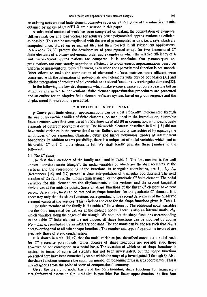
2.1 The Co family The first three members of the family are listed in Table 1. The first member is the well

known “constant strain triangle”, the nodal variables of which are the displacements at the vertices and the corresponding shape functions, in triangular coordinates, are L,, Lz, Ls. (References [16] and [19] present a clear interpretation of triangular coordinates.) The next member of the family is the “linear strain triangle” or the quadratic c finite element. The nodal variables for this element are the displacements at the vertices and the second tangential derivatives at the midside points. Since all shape functions of the linear Co element have zero second derivatives, they can be retained as shape functions for the quadratic (? element. It is necessary only that the shape functions corresponding to the second derivatives of the quadratic element vanish at the vertices. This is indeed the case for the shape functions given in Table 1.

The third member of the family is the cubic p finite element. The additional nodal variables are the third tangential derivatives at the midside nodes. There is also an internal mode, Nlo, which vanishes along the edges of the triangle. We note that the shape functions corresponding to the cubic Co finite element are not unique; all shape functions can be modified by adding Nlo = L1L2L3 multiplied by an arbitrary constant. The constants can be chosen such that Nlo is energy-orthogonal to all other shape functions. The number and type of operations involved.are precisely those of static condensation.

It is shown in Refs. [16,19] that the nodal variables just described constitute a nodal basis for C? piecewise polynomials. Other choices of shape functions are possible also, those however do not correspond to a nodal basis. The question of which set of shape functions is optimal in terms of numerical stability has not been investigated, but the shape functions presented here have been numerically stable within the range of p investigated (1 through 8). Also, the shape functions comprise the minimum number of monomial terms in area coordinates. This is advantageous from the point of view of computational economy.

Given the hierarchic nodal basis and the corresponding shape functions for triangles, a straightforward extension for tetrahedra is possible: For linear approximation the first four

B. A. SZABO

Table 1. Nodal variables and shape functions for the first three hierarchic triangular C” elements

3 terms: Values of the approximating polynomial at the vertices.

Normalizing factor: I

N,=L,, Nz=Lz, N,=L,

3 additional terms: Second derivatives of the approximating polynomial at the vertices.

Normalizing factor: -l/2

Nd=L,Lz, Ns=LzL,, Ng=L,L,

3. Cubic 4 additional terms: Three third derivatives of the approximating polynomial at the midpoints of edges.

Normalizing factor: l/l2

N,= L,‘L2-L,Lr2, NE = Lz’L, - LzL,~, Ns = L,2L, - L,‘L,

One internal mode:

NIO = LL2L3

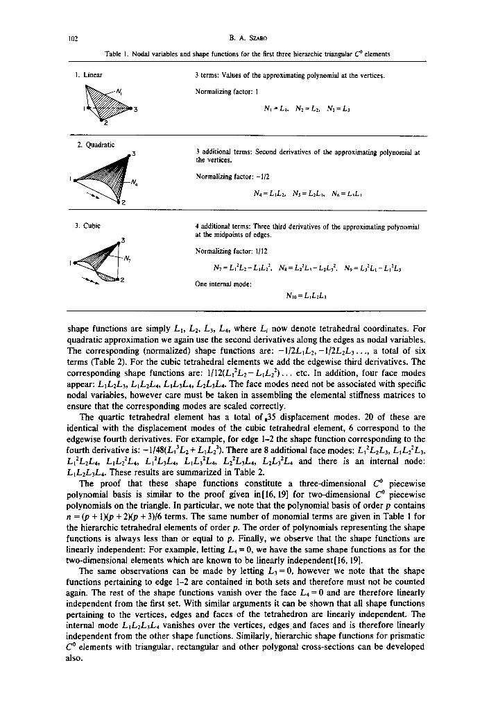
shape functions are simply L,, Lz, Lj, L4, where Li now denote tetrahedral coordinates. For quadratic approximation we again use the second derivatives along the edges as nodal variables. The corresponding (normalized) shape functions are: -1/2LiL~, -1/2L2L3.. ., a total of six terms (Table 2). For the cubic tetrahedral elements we add the edgewise third derivatives. The corresponding shape functions are: 1/12(Li*L2- LiLz*). . . etc. In addition, four face modes appear: LiLzL3, LILzL4, LIL3L4, L2L3L4. The face modes need not be associated with specific nodal variables, however care must be taken in assembling the elemental stiffness matrices to ensure that the corresponding modes are scaled correctly.

The quartic tetrahedral element has a total of $5 displacement modes. 20 of these are identical with the displacement modes of the cubic tetrahedral element, 6 correspond to the edgewise fourth derivatives. For example, for edge l-2 the shape function corresponding to the fourth derivative is: -1/48(Lr3L2+ L3Lz3). There are 8 additional face modes: L12L2L3, LIL2*L3,

Li2L2L4, LIL2*L4, L12L3L4, LIL3*L4, Lz2L3L4, LtL3*L4 and there is an internal node: LiL2L3L4. These results are summarized in Table 2.

The proof that these shape functions constitute a three-dimensional Co piecewise polynomial basis is similar to the proof given in[ 16,191 for two-dimensional C3 piecewise polynomials on the triangle. In particular, we note that the polynomial basis of order p contains n = (p + I)(p + 2)(p + 3)/6 terms. The same number of monomial terms are given in Table 1 for the hierarchic tetrahedral elements of order p. The order of polynomials representing the shape functions is always less than or equal to p. Finally, we observe that the shape functions are linearly independent: For example, letting L4 = 0, we have the same shape functions as for the two-dimensional elements which are known to be linearly independent[l6,19].

The same observations can be made by letting L3 = 0, however we note that the shape functions pertaining to edge l-2 are contained in both sets and therefore must not be counted again. The rest of the shape functions vanish over the face L4 = 0 and are therefore linearly independent from the first set. With similar arguments it can be shown that all shape functions pertaining to the vertices, edges and faces of the tetrahedron are linearly independent. The internal mode LIL2L3L.4 vanishes over the vertices, edges,and faces and is therefore linearly independent from the other shape functions. Similarly, hierarchic shape functions for prismatic C3 elements with triangular, rectangular and other polygonal cross-sections can be developed also.

Some recent developments in finite element analysis

Table 2. Nodal variables and shape functions for the first four hierarchic tetrahedral r? elements

103

4 3

Liz3 \ 2

1. Linear 4 terms: Values of the approximating function at the vertices.

N,= L,, Nz= Lz, N3= Ls, Nq= L,

2. Quadratic 6 additional terms: Second derivatives at the midpoints of edges.


Ns = L,Lz, Ne = LzL,. . . . NIO = LIL,

3. Cubic 10 additional terms: Six third derivatives at the midpoints of edges.

. I Normahzmg factor: 5

N,,=L,2L2-L,L;, N,,= L;L,-LzL?, . . . NM.=LI~L,-L,L~

Four face modes: 1

N,, = L,LzL~, N,s = LILZLC NW = L,L,Lc Nm = L2&4

4. Quartic 15 additional terms: Six fourth derivatives at the midpoints of edges.


N2, = L,3L2+ L,L>: Nz = Lz’L, + LzL,‘, . . . Nz= L,‘L,+ LIL,~

Eight face modes:

N2, = L,‘LzL,, Nts = L,Lz2L3, Nn = L12L2L Na = LIL~~L,,

N3, = L,2L,Ld, N32 = L,L,‘L,, NJ, = Lg*L,L,, Nw = LzL?L.

One internal mode:

N~s = L&zL&

2.2 The C’ family The subject of hierarchic C’ elements is best approached by first examining two complete,

exactly and minimally conforming non-hierarchic finite elements which preceded the development of the hierarchic C’ finite elements. Such developments were clearly motivated by. the desire to avoid problems caused by overconforming elements in approximating certain boundary and connectivity conditions such as those that occur at reentrant corners, sudden changes in plate thickness, shell intersections, etc.

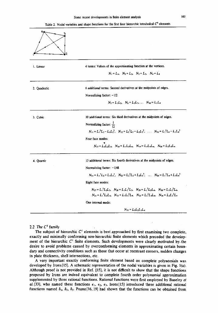
A very important exactly conforming finite element based on complete polynomials was developed by Irons[lS]. A schematic representation of the nodal variables is given in Fig. l(a). Although proof is not provided in Ref. [IS], it is not difficult to show that the shape functions proposed by Irons are indeed equivalent to complete fourth order polynomial approximation supplemented by three rational functions. Rational functions were first employed by Baseley et al. [33], who named these functions 61, EZ, ~3. Irons[lS] introduced three additional rational functions named Sr, 62, 83. Peano[l6,19] had shown that the functions can be obtained from

104 B. A. SZABO

simple combinations of a new set of rational functions, called vi, Q, . . ., q6:

The sums (7, + 77~)~ (773 + 774), (75 + 376) yield three quartic monomial terms. The c’s are given by:

El=q3+q5, E2=q2+%, E3=77,+774

and the S’s are given by[32]:

b=‘13-775, aZ=“rl2-% 83=7,,-7)4.

Thus the three independent rational functions which supplement the complete quartic polynomial in Irons’ quartic element are: (7, - n2), (773 - ?74), (r/5 - 776). The q functions have further significance: they are the shape functions associated with the mixed second partial derivatives, taken along the sides and normal to the sides of a triangle and evaluated at the vertices [ 16, 19,341.

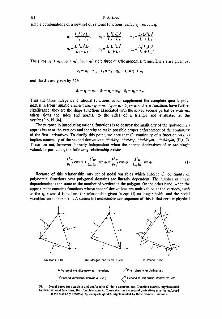
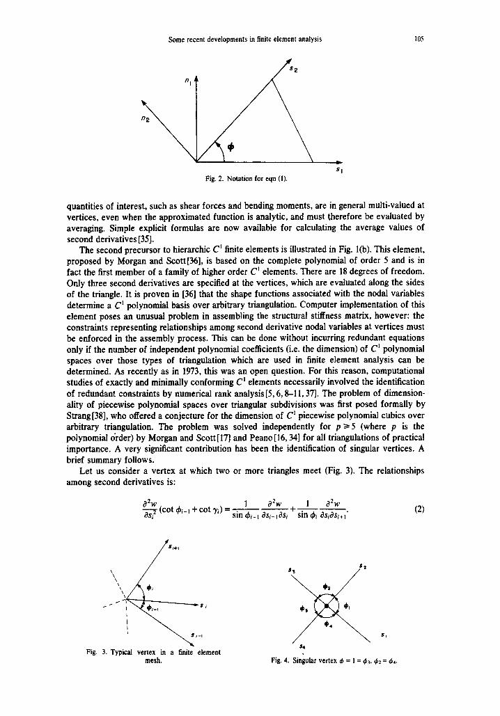
The purpose in introducing rational functions is to destroy the analiticity of the (polynomial) approximant at the vertices and thereby to make possible proper enforcement of the continuity of the first derivatives. To clarify this point, we note that C’ continuity of a function w(x, y) implies continuity of the second derivatives: ~*w/&~~, a*~/&~*, a2w/aslanl, a2wlas2dn2 (Fig. 2). These are not, however, linearly independent when the second derivatives of w are single valued. In particular, the following relationship exists:

2 2

gbs++&- I I I

sin4 =$cosr$- 2

ssind. (1)

Because of this relationship, any set of nodal variables which enforce C’ continuity of polynomial functions over polygonal domains are linearly dependent. The number of linear dependencies is the same as the number of vertices in the polygon. On the other hand, when the approximant contains functions whose second derivatives are multivalued at the vertices, such as the n, E and 6 functions, the relationship given in eqn (1) no longer holds, and the nodal variables are independent. A somewhat undesirable consequence of this is that certain physical

(a, Irons Cl51 lb) Morgan and Scott C361 (cl Rsano C I61

l Value of the displacement function; /First directional derivative;

f Second directional derivative, etc.;

0 Second mixed portial derivative, etc.

Fig. I. Nodal bases for complete and conforming C’ finite elements. (a). Complete quartic, supplemented by three rational functions; (b), Complete quintic. Constraints on the second derivatives must be enforced

in the assembly process; (c), Complete quintic, supplemented by three rational functions.


Fig. 2. Notation for eqn (I).

quantities of interest, such as shear forces and bending moments, are in general multi-valued at vertices, even when the approximated function is analytic, and must therefore be evaluated by averaging. Simple explicit formulas are now available for calculating the average values of second derivatives [35].

The second precursor to hierarchic C’ finite elements is illustrated in Fig. l(b). This element, proposed by Morgan and Scott[36], is based on the complete polynomial of order 5 and is in fact the first member of a family of higher order C’ elements. There are 18 degrees of freedom. Only three second derivatives are specified at the vertices, which are evaluated along the sides of the triangle. It is proven in [36] that the shape functions associated with the nodal variables determine a C’ polynomial basis over arbitrary triangulation. Computer implementation of this element poses an unusual problem in assembling the structural stiffness matrix, however: the constraints representing relationships among second derivative nodal variables at vertices must be enforced in the assembly process. This can be done without incurring redundant equations only if the number of independent polynomial coefficients (i.e. the dimension) of C’ polynomial spaces over those types of triangulation which are used in finite element analysis can be determined. As recently as in 1973, this was an open question. For this reason, computational studies of exactly and minimally conforming C’ elements necessarily involved the identification of redundant constraints by numerical rank analysis[5,6,&11,37]. The problem of dimensionality of piecewise polynomial spaces over triangular subdivisions was first posed formally by Strang [38], who offered a conjecture for the dimension of C’ piecewise polynomial cubits over arbitrary triangulation. The problem was solved independently for p 2 5 (where p is the polynomial order) by Morgan and Scott [ 171 and Peano [ 16,341 for all triangulations of practical importance. A very significant contribution has been the identification of singular vertices. A brief summary follows.

Let us consider a vertex at which two or more triangles meet (Fig. 3). The relationships among second derivatives is:

2 1 CY2W 1 a2w $(COt4i-j+COtR)=-- --

sin 4i-1 a&-l& + sin di as&i+r’

Fig. 3. Typical vertex in a fmite element mesh. Fig. 4. Singular vertex $ = 1 = 4,. C& = 6,.

106 B. A. SZABO

This constraint must be enforced in the process of assembling the structural stiffness matrix when the nodal basis proposed by Morgan and Scott is employed. A detailed discussion of this point can be found in [16,34]. A singular vertex occurs when four edges meet at a vertex and 4i= 63, 4~ = 1$4 (Fig. 5). In this case cot 4i-r + cot 4i = 0 and the relationship, given in eqn (2), enforced around the vertex, results in four homogeneous algebraic equations among the mixed second derivatives, one of which is redundant. In order to avoid such redundancies, one of the four constraints must not be enforced when a singular vertex is encountered.

The first member of the hierarchic family of C’ elements is illustrated in Fig. l(c). The element has 24 degrees of freedom, and its basis is equivalent to the complete fifth-order polynomial supplemented by the same three rational functions as Irons’ quartic element[l5]. For full description of this element, the reader is referred to the original expositions[l6,19,34]. Shape functions are available for higher-order hierarchic ,C’ elements as well.

As a practical matter, the importance of C’ plate and shell elements has decreased considerably with the introduction of numerically stable and efficient Co plate bending elements. Hierarchic c plate bending elements have been implemented in the experimental computer program, COMET-X[26]. Computational studies have shown the elements to be stable at least over the range of polynomial orders I-8 permitted by COMET-X.

3. RATE OF p-CONVERGENCE

Important advances have been made in the understanding of the p-convergence process in finite element approximation of elliptical boundary value problems. The results, briefly summarized in the following, have practical significance in that they establish p-convergence as a feasible and attractive method for achieving improved accuracy in adaptive finite element computations and provide an independent method for computing certain quantities of interest.

The rapid convergence in energy as well as pointwise convergence of finite element approximations employing high order finite elements, when the approximated function is smooth, has been recognized ‘by several investigators [5,7,9, Wl]. In practical problems, however, the approximated function is very seldom smooth. In the large majority of cases, the lack of smoothness is due to angular corners at external boundaries. In two dimensional elasticity, for example, the displacement vector components at corners are of the form:

ui = r”gi(O) + Gi(r, 6) (3)

in which i = 1,2; r and 0 are polar coordinates with the origin at the corner; Y > l/4, its value depends on the comer angle and the boundary conditions imposed at the corner; gi and Gr are smoother functions than Ui in the neighborhood of r = 0. The values of v for plane elastic and plate problems are given in [42].

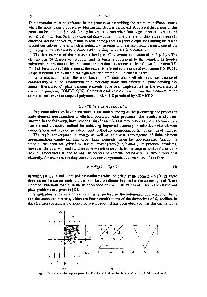
Singularities, such as a comer singularity, perturb fir, the polynomial approximation to Ui, and the computed stresses, which are linear combinations of the derivatives of iii, oscillate in the elements containing the source of perturbation. It has been observed that this oscillation is

(a) (b) (cl

Fig. 5. Centrally cracked square panel. (a), Problem definition; (b), E-Element mesh; (c), 3-Element mesh.


similar to the oscillation of Fourier series in the vicinity of jump discontinuities, in the sense that the average of successive partial sums (the first Cesaro sums) of the computed stresses approximate the true stress distribution with increasing precision as the order of polynomial approximation is increased [21,23,43]. This phenomenon has not been studied in detail and it certainly deserves further attention. However, obtaining close pointwise stress approximation in the vicinity of singularities is not necessary in stress analysis. Of primary importance is that the true energy density distribution be closely approximated in the finite element solution and the singularity should not significantly perturb the displacement and stress approximations in elements away from the crack tip. It has been demonstrated that rapid convergence in energy occurs when the polynomial displacement approximation is progressively increased on a fixed finite element mesh [22,23,43] and the stress oscillations caused by singularities are confined to the elements in the immediate vicinity of the singularities [23,43].

From the point of view of designing an adaptive finite element software system, it is important to consider the rate of (energy) convergence. When the number of degrees of freedom, N, is increased through uniform (or locally uniform) mesh refinement then the energy error is bounded by:

in which U is the exact strain energy; 0 is the computed strain energy; c is a constant which depends on the order p of the polynomial approximation, the value of the elastic constants and the geometry of the mesh, Y* = min (v, p) [44].

In contrast, when the number of degrees of freedom is increased through increasing the order of polynomial approximation, the error in strain energy is bounded by:

u-o+&. E > 0 arbitrary

in which k is a constant which depends only on the elastic constants, the geometry of the mesh and the distribution of polynomial orders over the mesh. The rate of convergence relationship expressed in eqn (5) was discovered in numerical experiments[22] and subsequently verified and generalized theoretically [25]. Thus, it has been established that the rate of p-convergence is twice the rate of h-convergence when corner singularities are present and the number of degrees of freedom are increased by uniform or quasi-uniform mesh refinement in the h-convergence process.

Numerical studies have indicated that the energy error is closely approximated by the bound given in eqn (5), even when the number of degrees of freedom is small. This is illustrated by an example, involving the centrally cracked square panel shown in Fig. 5(a). Due to symmetry, only one quarter of the panel had to be analyzed. Two finite element meshes were used: the eight-element mesh (Fig. 5b) and the three-element mesh (Fig. 5c) which comprises the minimum number of elements needed for describing the geometry for this problem. In the eight element mesh the polynomial orders of the displacement approximation were distributed in two ways: uniformly and non-uniformly. In the non-uniform or graded distribution the polynomial orders were increased over p = 3 only in the crack tip elements (numbered 1, 3, 4); the polynomial order was constant at p = 3 in the remote elements (numbered 5, 6, 8) and the transition elements (numbered 2, 7). However, in order to preserve completeness of the polynomial approximating functions in the crack tip elements, as well as Co continuity, it was necessary to add higher order shape functions to the transition elements corresponding to the higher order hierarchic nodal variables at their interelement boundaries with the crack tip elements.

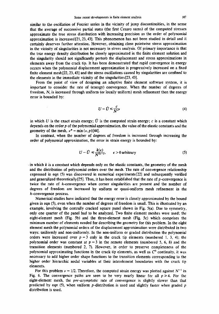
For this problem v = l/2. Therefore, the computed strain energy was plotted against N-’ in Fig. 6. The convergence paths are seen to be very nearly linear for all p a 4. For the eight-element mesh, the pre-asymptotic rate of convergence is slightly slower than that predicted by eqn (5), when uniform p-distribution is used and slightly faster when graded p distribution is used.

B. A. SZABO

1

0.750 Y

0.740 -

0.720’ ’ ’ I I t I I I 1 I I I,, I 1 ,

I 2 3 4 5 6 7 6 9 IO II 12 13 Y IS I6 17

1000/N Fig. 6. Centrally cracked panel. Computed strain energy (quarter panel only) for varying polynomial orders

(p) vs reciprocal of the net degrees of freedom. E, modulus of elasticity; t, Panel thickness.

The bound given by eqn (5) is sufficiently close within the range of mesh divisions and polynomial orders that can be employed in practical computations to permit estimation of the exact strain energy by extrapolation to well within one per cent of accuracy. For example, let us define o,, as an estimate of U based on eqn (5):

0

P

= NpZVOp - NC, ir,_, Np2' -N:'-, (6)

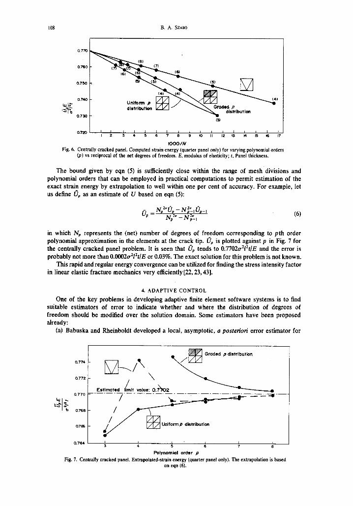
in which Np represents the (net) number of degrees of freedom corresponding to pth order polynomial approximation in the elements at the crack tip. 4 is plotted against p in Fig. 7 for the centrally cracked panel problem. It is seen that 4 tends to 0.7702a212t/E and the error is probably not more than 0.0002u212?/E or 0.03%. The exact solution for this problem is not known.

This rapid and regular energy convergence can be utilized for finding the stress intensity factor in linear elastic fracture mechanics very efficiently [22,23,43].

4. ADAPTIVE CONTROL

One of the key problems in developing adaptive finite element software systems is to find suitable estimators of error to indicate whether and where the distribution of degrees of freedom should be modified over the solution domain. Some estimators have been proposed already:

(a) Babuska and Rheinboldt developed a local, asymptotic, a posterion’ error estimator for

Graded p dlstrlbution

0.764 I I I I 1 I 3 4

I 5 6 7 6

Polynomial order p Fig. 7. Centrally cracked panel. Extrapolated-strain energy (quarter panel only). The extrapolation is based

on eqn (6).


h-convergent approximations [4]. The estimator requires element level computations only and measures the error in strain energy associated with an element. An optimal distribution of the degrees of freedom is obtained when this error measure is the same for all elements.

(b) Melosh and Marcal[45] proposed to measure the specific energy difference (SED), defined as the largest difference over the element domain between the computed strain energy density function and the same function evaluated at the origin of the elemental coordinate system. This measures the effect of modes, higher than those associated with the (generalized) constant strain states, on the distribution of strain energy density within finite elements. The criterion for mesh refinement is that SED be approximately the same for each finite element. In practical computations SED is approximated by the largest of the strain energy density differences evaluated at quadrature points only.

(c) Peano et al. [28,46] proposed a criterion for p-convergent approximations. This criterion is based on the rate of change of the total potential energy with respect to higher order displacement modes, evaluated before the higher displacement modes are actually introduced When the rate of change of the potential energy exceeds a prescribed tolerance, the stiffness terms corresponding to the higher modes are assembled and the new system or equations is solved. The hierarchic structure of the elemental stiffness matrices permits efficient use of block relaxation procedures in obtaining improved solutions.

(d) In Refs. [47,48], investigation of error estimators, similar to the estimators proposed by Babuska and Rheinboldt[4] but modified for p-convergent approximations, was reported. The results of these investigations are reviewed in the following:

Two estimators were defined. One, called the r-estimator, is a function of the unbalanced body forces within individual elements:

&jrirjWk(t dA)

in which: Ak is the area of the kth element; pk is the polynomial order of the displacement approximation over the kth element; a is a constant, determined by numerical experiments; E is the modulus of elasticity; Sij is the Kronecker delta; ri is the unbalanced body force vector component: ri = G& + (A + G)& + Xi. G and A are Lami’s parameters; iii is the ith component of the displacement vector computed by the finite element method; Xi is the imposed body force); wk is a weight function; and t is the panel thickness.

The other estimator, called the t-estimator, is a function of the unbalanced tractions at interelement boundaries:

(8)

in which: /3 is a constant, determined by numerical experiments; rk denotes the kth element boundary; ti is the vector of unbalanced tractions: ti = [&j”(s) - &l!‘(s)Jnj (S is the coordinate along the interelement boundary, S$) is the finite element solution for the stress tensor for the ath element, nj is the unit normal to the interelement boundary between elements a and b); Ok is a weight function.

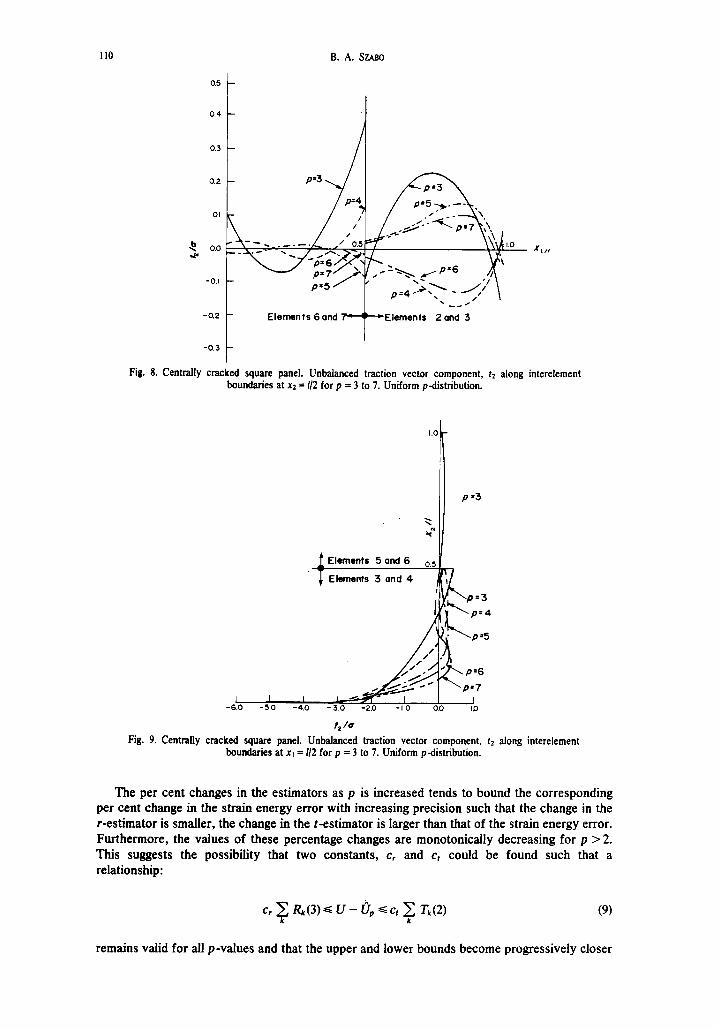
The typical variation of fi with increasing polynomial orders along interelement boundaries is illustrated in Figs. 8 and 9. In Fig. 8 the variation of t2 at x2 = l/2 is shown for the centrally cracked square panel discussed in the preceding section and shown in Fig. 5. Uniform pdistribution was employed. t2 attenuates rather slowly, however the signs alternate for even and odd p values indicating that the rate of attenuation of t2 can be increased by averaging.

The variation of tt along XI = l/2 is shown in Fig. 9. The attenuation of t2 between elements 5 and 6 is so rapid that only the value for p = 3 can be shown at the scale of this diagram. There is no appreciable attenuation on the other hand between the crack tip elements. Successive averaging smoothens f2 and shifts the peak progressively closer to the crack tip.

The computed dimensionless strain energy values, the corresponding errors and the values of the two error estimators for parameter values a = 3, p = 2 and weight function values wk = Wk = 1 are given in Table 3.

CAMWA. Vol. 5. No. 1-C

110 B. A. SZMO

t

Elements 6 and Elements 2and 3

-0.3

t

Fig. 8. Centrally cracked square panel. Unbalanced traction vector component, cz along interelement boundaries at xz = l/2 for p = 3 to 7. Uniform p-distribution.

1.0

” : p=3

3 c

Elements 5 and 6 o,5

Elements 3 and 4

Fig. 9. Centrally cracked square panel. Unbalanced traction vector component, f2 along interelement boundaries at x, = l/2 for p = 3 to 7. Uniform p-distribution.

The per cent changes in the estimators as p is increased tends to bound the corresponding per cent change in the strain energy error with increasing precision such that the change in the r-estimator is smaller, the change in the t-estimator is larger than that of the strain energy error. Furthermore, the values of these percentage changes are monotonically decreasing for p > 2. This suggests the possibility that two constants, c, and c, could be found such that a relationship:

k k (9)

remains valid for all p-values and that the upper and lower bounds become progressively closer

Some recent developments in finite element analysis

Table 3. Estimators for the error in strain energy. Cen- trally cracked panel, 8-clement mesh, uniform pdis-

tributiont

2 0.6936 0.0766 0.01080 0.0305 3 0.7305 0.0397 0.00668 0.0189 4 0.7461 0.0241 0.00401 0.0113 5 0.7538 0.0164 0.00273 0.0077 6 0.7584 0.0118 0.00201 0.0057 7 0.7613 0.0089 0.00158 0.0045

tTo convert entries into dimensioned values, multiply by a*1*t/E. Poisson’s ratio: 0.3.

to the strain energy error as p is increased. This is, of course, highly speculative at the present because no theoretical justification exists, but consistent with the observations of this numerical experiment. For example, if we choose C, = 5.633 and c, = 0.748, the two estimators will give the value of the strain energy error at p = 7. The resulting relationship between the strain energy error and the two estimators is illustrated in Fig. 10.

Similar results were obtained in other computational experiments in which the strength of corner singularity, as characterized by u, was varied[48]. Thus, the indications are that the r

and t estimators give respective lower and upper bounds for the strain energy error regardless of the strength of corner singularity.

The question naturally arises whether the same estimators would bound the energy error at the element level as well. Clearly, this approach will be useful only if the indicators tend to zero with increasing p at about the same rate as the error in strain energy does, not only for the entire solution domain but for individual finite elements as well. Study of the local error in the energy norm is complicated by the fact that the local error can be computed only if the exact solution is known. Studies concerned with the local behavior of the estimators are in progress. The available results indicate that the element to element variation of the r and t estimators conforms closely with the probable error variation in strain energy, indicating that the r and t

Fblynomlol order, p

‘0.05

0.04

0.03

QO2

0.01

/ / 0.0 I I I I I I

0.0 2.0 4.0 6.0 60 10.0 120

IOOWN

Fig. 10. Centrally cracked square panel. Energy error and energy error estimators vs reciprocal of the net number of degrees of freedom. The estimators were multiplied by suitable scaling constants.

112 B. A. .%?ABO

estimators or similar estimators may provide a suitable basis for adaptive redistribution of the degrees of freedom in finite element analysis.

5. ADAPTIVE FINITE ELEMENT SOFTWARE SYSTEM BASED ON p-CONVERGENCE

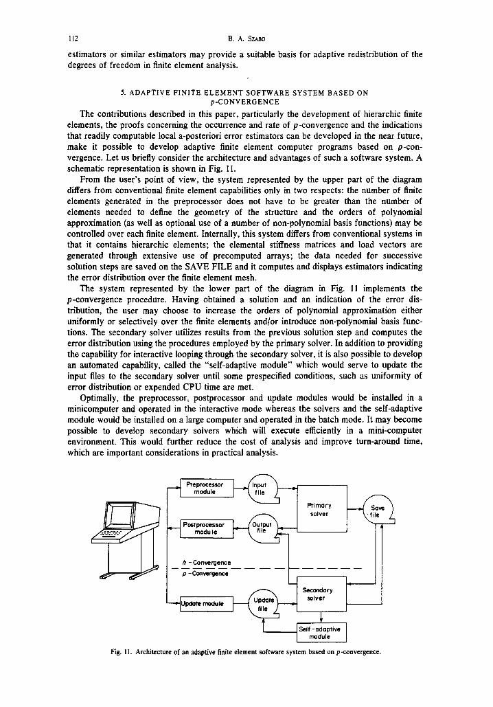
The contributions described in this paper, particularly the development of hierarchic finite elements, the proofs concerning the occurrence and rate of p-convergence and the indications that readily computable local a-posteriori error estimators can be developed in the near future, make it possible to develop adaptive finite element computer programs based on p-convergence. Let us briefly consider the architecture and advantages of such a software system. A schematic representation is shown in Fig. 11.

From the user’s point of view, the system represented by the upper part of the diagram differs from conventional finite element capabilities only in two respects: the number of finite elements generated in the preprocessor does not have to be greater than the number of elements needed to define the geometry of the structure and the orders of polynomial approximation (as well as optional use of a number of non-polynomial basis functions) may be controlled over each finite element. Internally, this system differs from conventional systems in that it contains hierarchic elements; the elemental stiffness matrices and load vectors are generated through extensive use of precomputed arrays; the data needed for successive solution steps are saved on the SAVE FILE and it computes and displays estimators indicating the error distribution over the finite element mesh.

The system represented by the lower part of the diagram in Fig. 11 implements the p-convergence procedure. Having obtained a solution and an indication of the error distribution, the user may choose to increase the orders of polynomial approximation either uniformly or selectively over the finite elements and/or introduce non-polynomial basis functions. The secondary solver utilizes results from the previous solution step and computes the error distribution using the procedures employed by the primary solver. In addition to providing the capability for interactive looping through the secondary solver, it is also possible to develop an automated capability, called the “self-adaptive module” which would serve to update the input files to the secondary solver until some prespecified conditions, such as uniformity of error distribution or expended CPU time are met.

Optimally, the preprocessor, postprocessor and update modules would be installed in a minicomputer and operated in the interactive mode whereas the solvers and the self-adaptive module would be installed on a large computer and operated in the batch mode. It may become possible to develop secondary solvers which will execute efficiently in a mini-computer environment. This would further reduce the cost of analysis and improve turn-around time, which are important considerations in practical analysis.

h -Conwqence ---_-----

p -Conwqenca

Primory n solver

Secondary solver

Fig. 11. Architecture of an adaptive finite element software system based on p-convergence.


Development of an adaptive finite element software system based on p-convergence yields the following significant advantages:

(a) A very large finite element library is available. Elements of any polynomial order can be used and the polynomials can be supplemented with non-polynomial basis functions.

(b) The number of finite elements is determined by the geometry rather than the considerations of accuracy.

(c) The distribution and number of degrees of freedom can be modified with minimal interactive and computational effort. Mesh refinement is not involved and the effort expended in triangularizing the stiffness matrix is saved for successive analyses (Hierarchical property).

(d) Very rapid energy convergence is obtained when the orders of polynomial approximation are increased on a fixed mesh even when the approximated function is not smooth, provided that discontinuities in loading, angular corners in boundaries and, in general, the sources of perturbation are located at interelement boundaries or vertices. This restriction is an acceptable one in most practical analyses.

(e) p-Convergence provides an efficient new method for computing stress intensity factors in linear elastic fracture mechanics.

(f) Based on the available information, it is estimated that in comparison with state-of-the- art methods, an order of magnitude reduction can be realized in the overall cost and time required for performing stress analysis tasks.

6. SOME UNSOLVED PROBLEMS

Until quite recently, convergence in finite element approximation was generally understood to mean h-convergence only. In the three fundamental aspects of the method: conditions for convergence to occur; asymptotic estimates for the rate of convergence and local, a-posteriori estimates of error distribution in various norms, a penetrating and elaborate mathematical support exists for h-convergent approximations. Adequate mathematical support now exists for p-convergent approximations in the fist two areas although some open questions still remain. In the third area, initial studies have indicated that readily computable a poster-hi error bounds that approach zero at about the same rate as the total error in strain energy exist but theoretical support is still lacking. The relationship between the local error and local error indicators is yet to be explored. This is perhaps the most important uncharted area in the theory of the finite element method.

There are other challenging problems as well: one concerns obtaining pointwise stress estimates in the neighborhood of singularities. It is known that averaging the stress solutions that result from progressively increasing orders of polynomial approximation on a fixed finite element mesh can smoothen the stress oscillations caused by singularities but techniques for optimal stress smoothing have not yet been developed.

Development of efficient secondary solvers is yet another unsolved problem. Block relaxation procedures have been employed and the results were found to be quite satisfactory: only very few iterations were needed [27,283. This subject deserves a systematic study, however, with particular reference to developing secondary solvers designed to operate on minicom- puters or in small partitions of large timesharing systems.

Extension of the convergence rate studies to three-dimensional problems in elasticity, particularly for studying problems posed by linear elastic fracture mechanics, is yet another promising area for research. Computational as well as theoretical studies are needed. Work in this area is currently in progress. For example, hierarchic shape functions of prismatic finite elements have been developed and implemented [49,50].

Application of adaptive finite element approximation methods based on p-convergence to non-linear problems is a completely unexplored area. The advantages of having a capability to adjust the distribution of degrees of freedom without mesh refinement and dealing with substantially fewer variables that require global operations, are likely to outweigh the disad- vantage of having to employ high order quadrature rules in generating elemental stiffness matrices. A particularly important computational problem in non-linear mechanics is posed by recent developments in the understanding of ductile fracture processes, which require evalua- tion of two energy related quantities, known as the “J-integral” and the “tearing modulus”,

114 B. A. Sweo

which measure the effect of crack length increments on the potential energy of non-linearly elastic solids 15 1,521.

7.SUMMARYANDCONCLUSIONS

The present state of development of a new finite element approximation procedure has been reviewed. In this procedure the finite element mesh is fixed and the number or type of basis functions is varied over the mesh, either uniformly or selectively, until some desired level of precision is reached. The basis functions are complete polynomials, optionally supplemented by rational or other non-polynomial basis functions. They are hierarchic, i.e. the set of basis functions associated with an element is a subset of the basis functions associated with each higher order element of the same kind. Consequently, the stiffness matrix of each element is embedded in the stiffness matrices of all higher order elements of the same kind. There are several computational advantages, the most important of which are that the rate of convergence is much faster than the rate of convergence achieved through mesh refinement and the number and distribution of degrees of freedom can be modified without sacrificing the effort spent on triangularizing the initial stiffness matrix. Thus the approximation error can be efficiently controlled.

It is concluded that development of adaptive finite element software systems, in which redistribution of the degrees of freedom is achieved through controlling the number and type of basis functions, is feasible. Such systems are likely to be more efficient, by an order of magnitude or more, than conventional finite element software systems.

Acknowledgements-The material surveyed here is the result of several years of effort of many investigators. The writer is particularly indebted to Professor Ivo Babuska of the University of Maryland, Dr. Albert0 Peano of the Polytechnic University of Milan and his colleagues at Washington University, Drs. I. N. Katz, M. P. Rossow and P. K. Basu for their contributions. Various phases of work on p-convergent approximations have been supported bv the National Science Foundation, the U.S. Department of Transportation,-the Association of American Railroads, AMCAR Division of ACF Industries, the Air Force Office of Scientific Research and the Electric Power Research Institute through giants and contracts awarded to Washington University.

REFERENCES I. I. Babuska. IIre Self-adaptive Approach in the Finite Element Method, ‘Ihe Mathematics of Finite Elements and

Applications II (Edited by J. R. Whiteman), pp. 125-142. Academic Press, New York (1976). 2. I. Babuska and W. C. Rheinboldt, Computational Aspects of the Finite Element Method. Mathematical Software 3,

225-25s (1977). 3. I. Babuska and W. C. Rheinboldt. Error Estimates for Adaptive Finite Element Computations. Technical Note BN-854,

Inst. for Physical Science and Technology, University of Maryland (May 1977). 4. 1. Babuska and W. C. Rheinboldt, A-Posteriori Error Estimates for the Finite Element Method. Tech. Rep. ‘JR-581,

University of Maryland (Sept. 1977). 5. Chung-Ta Tsai, Analysis of Plate Bending by the Quadratic Programming Approach. Doctoral Dissertation, Washing-

ton University, St. Louis, Missouri (1971). 6. B. A. Sxabo and Chung-Ta Tsai, The Quadratic Programming Approach to the Finite Element Method. Int. 1. Num.

Meth. Engng 5.375-381 (1973). 7. K. C. Chen, High-Precision Finite Elements for Plane Elastic Problems. Doctoral Dissertation, Washington University,

St. Louis, Missouri (1972). 8. J. H. Paliwala, Plate Stability Analysis by the Constraint Method. Doctoral Dissertation, Washington University, St.

Louis, Missouri (1974). 9. C. W. Godbold, Convergence Characteristics of Cylindrical Shell Finite Elements. Doctoral Dissertation, Washington

University, St. Louis, Missouri (1972). IO. Chung-Ta Tsai and B. A. Sxabo, The Constraint Method-A New Finite Element Technique. NASA Technical

Memorandum, NASA TM X-2893.551-568 (Sept. 1973). II. Il. A. Szabo, K. C. Chen and Chung-Ta Tsai, Conforming Finite Elements Based on Complete Polynomials. Comp.

Struct. 4, 521-530 (1974). 12. B. A. Sxabo and T. Kassos, Linear Equality Constraints in Finite Element Approximation. fnt. J. Num. Met/r. Engng 9,

563-580 ( 1975). 13. M. P. Rossow, K. C. Chen and J. C. Lee, Computer Implementation of the Constraint Method. Comp. Struct. 6,

203-209 (1976). 14. P. C. Dunne, Complete Polynominal Displacement Field for Finite Element Method. Awn. J. Royal Aeron. Sot. 72,

245-247 (1968) and discussions of the paper. IS. B. M. Irons, A Conforming Quartic Triangular Element for Plate Bending. Int. .I. Num. Met/t. Engng 1, 29-45 (1%9). 16. A. G. Peano, Hierarchies of Conforming Finite Elements. Doctoral Dissertation, Washington University, St Louis,

Missouri (1975). 17. J. Morgan and R. Scott, The Dimension of the Space of C’ Piecewise Polynomials. manuscript. 18. 0. C. Zienkiewicz, B. M. Irons, I. C. Scott and J. S. Campbell, Three Dimensional Stress Analysis. Froc. IUTAM

Symp. on High Speed Computing of Elastic Structures, Liege, Belgium, 1970, 1, 41-32 (1971).


21.

22.

23.

24. 25. 26.

21.

28.

29.

30.

31.

32.

33.

M. P. Rossow. A. K. Mehta and G. Petruska. First Cesaro Sums for Hind Order Finite Elements Near Sinmdarities. Short Communication. Int. 1. Num. Melhs. E&g 11.753-755 (1977). - B. A. Szabo and A. K. Mehta, p-Convergent Finite Element Approximations in Fracture Mechanics. Int. J. Num. Meths. Engng 12.551-560 (1978). A. G. Peano, B. A. Szabo and A. K. Mehta, Self-Adaptive Finite Elements in Fracture Mechanics. Comput. Methods Appl. Mech. Engng 16,69-g0 (1978). G. Petruska. Finite Element Convernence on Fixed Grid. Coma. Maths. with Appls. 4,67-71 (1978). I. Babuska, Private Communication-

. .

P. K. Basu, M. P. Rossow and B. A. Szabo, Theoretical Manual and Users’ Guide for COMET-X. Rep. FRAIORD- 77/60, Washington University (1977).

34. 35. 36.

31. 38. 39.

A. Pasini, A. Peano, R. Riccioni and R. Sardella, A Self-Adaptive Finite Element Analysis. 6th int. finite EIement Gong., Baden-Boden, FDR (l&l5 Nov. 1977). A. Peano, M. Fanelli, R. Riccioni and R. Sardella, Self-Adaptive Convergence at the Crack Tip of a Dam Buttress. Proc. Int. Conf. on Num. Meth. in Fracture Mechanics, Swansea, U.K. (P-13 Jan. 1978). 1. N. Katz, A. G. Peano and M. P. Rossow, Nodal Variables for Complete Conforming Finite Elements of Arbitrary Polynomial Order. Comp. & Maths. with Appls. 4,85-112 (1978). M. P. Rossow and I. N. Katz, Hierarchical Finite Elements and Precomputed Arrays. Int. 1. Num. Meth. Engng 12, 977-999 (1978). E. Y. Rodin, A New Method of Integration over Polynomial Finite Element Boundaries. Int. J. Num. Meth. Engng 8, 1115-I 124 (1976). I. N. Katz, Integration of Triangular Finite Elements Containing Corrective Rational Functions. Int. J. Num. Meth. Engng 11, 107-I 14 (1977). G. P. Baseley, Y. K. Cheung, B. M. Irons and 0. C. Zienkiewicz, Triangular Elements in Plate Bending-Conforming and Non-conforming Solutions. Proc. Conf. on Matrix Methods in Structural Mechanics, Wright Patterson AFB, Oct. I%5 (Report AFFDL-TR-66-80, pp. 547-576, Nov. 1966). A. G. Peano, Conforming Approximations for Kirchhoff Plates and Shells. Int. J. Num. Meth. Engng. to be published. I. N. Katz, Private Communication. J. Morgan and R. Scott, A Nodal Basis for C’ Piecewise Polynomials of Degree n > 5. Mathematics of Computation 29, 736-740 (1975). M. P. Rossow and A. K. Ibrahimkhail, Constraint Method Analysis of Stiffened Plates. Comput. Struct. 8,51-60 (1978). G. Strang, Piecewise Polynomials and the Finite Element Method. BUN. Am. Math. Sot. 79, 1128-l 137 (1973). G. R. Cowper, E. Kosko, G. Lindberg and M. Olson, Static and Dynamic Applications of a High Precision Triangular Plate Bending Element. AIAA 1. 7, 1957-1965 (1%9).

40. V. Hoppe, Finite Elements with Harmonic Interpolation Functions The Mathematics of Finite Elements and Applications (Edited by J. R. Whiteman), pp. 131-142. Academic Press, New York (1973).

41. C. Caramanlian, Finite Element Formulations in Plane Stress and Plate Bending. Doctoral Dissertation, University of Toronto (1975).

19. A. G. Peano, Hierarchies of Conforming Finite Elements for Plane Elasticity and Plate Bending. Camp. & Maths. with

Appls. 2,211-224 (1976). 20. G. Petruska, Private communication.

42. M. L. Williams, Stress Singularities Resulting from Various Boundary Conditions in Angular Comers of Plates in Extension. J. Appl. Mech. AShfE 526-528 (1952).

43. A. K. Mehta. oConveraent Finite Element Aooroximations in.Linear Fracture Mechanics. Doctoral Dissertation. Washington University $78).

. .

44. G. Strang and G. J. Fix, An Analysis of the Finite Element Method. Prentice Hall, Englewood Cliffs, New Jersey (1973).

45. R. J. Melosh and R. V. Marcal, An Energy Basis for Mesh Refinement of Solid Continua. Int. J. Num. Merh. Engng 11, 1083-1091 (1977).

46. A. G. Peano, Energy Gradient Technique for Adaptive Finite Element Analysis. 15th Ann. Meeting Sot. Engng Sci., Gainesoille, Florida (4-6 Dec. 1978).

47. B. A. Szabo, P. K. Basu and M. P. Rossow, Adaptive Finite Element Analysis Based on P-Convergence. Symposium on Furure Trends in Computerized Slrucrural Analysis and Synthesis, Washington, D.C., Nov. 1978. NASA Conference Publication 2059, pp. 43-50 (1978).

48. P. K. Basu and B. A. Szabo, Adaptive Control in P-Conuergent Approximations. Proc. 15th Annual Meeting, Sot. of Engineering Science, Gainesville, Florida, Dec. 1978.

49. I. N. Katz, A Hierarchical Family of Complete, Conforming Prismatic Finite Elements of Arbitrary Polynomial Order. SIAM 1978 National Meetina. Madison, Wisconsin (24-29 Mav 1978).

50. A Peano, A. Pasini, R. Ric&ni and L. Sardella, Adiptioe ApiroximcQions in Finite Element Srructuml Analysis and Synlhesis. Symposium on Future Trends in Computerized Structural Analysis and Synthesis, Washington, D.C., Nov. 1 1978. To be published in Comp. Struck

51. P. C. Paris, H. Tada, A. Zahoor and H. Ernst, A Treatment of the Subject of Tearing Instability. Rep. NUREG-0311, prepared for the Nuclear Regulatory Commission (Aug. 1977).

52. J. W. Hutchinson and P. C. Paris, Stability of Analysis of I-Controlled Crack Growth. ASTM Symposium on Elastic-Plastic Fracture, Atlanta, 1977, ASTM-STP 677 (1979).

Documents

SOME RECENT DEVELOPMENTS IN FINITE ELEMENT ANALYSIS … · SOME RECENT DEVELOPMENTS IN FINITE ELEMENT ANALYSIS B. A. SZABO Greensfelder Professor of Civil Engineering, Washington