SOME CLASSES OF GENERALIZED CYCLOTOMICPOLYNOMIALS

by

Abdullah Al-Shaghay

Submitted in partial fulfillment of the requirementsfor the degree of Doctor of Philosophy

at

Dalhousie UniversityHalifax, Nova Scotia

December 2019

c⃝ Copyright by Abdullah Al-Shaghay, 2019

Table of Contents

List of Tables . . . . . . . . . . . . . . . . . . . . . . . . . . . . . . . . . . . vi

List of Figures . . . . . . . . . . . . . . . . . . . . . . . . . . . . . . . . . . vii

Abstract . . . . . . . . . . . . . . . . . . . . . . . . . . . . . . . . . . . . . . viii

List of Abbreviations and Symbols Used . . . . . . . . . . . . . . . . . . ix

Acknowledgements . . . . . . . . . . . . . . . . . . . . . . . . . . . . . . . x

Chapter 1 Introduction . . . . . . . . . . . . . . . . . . . . . . . . . . 1

Chapter 2 Cyclotomic Subgroup-Polynomials . . . . . . . . . . . . . 3

2.1 Preliminaries . . . . . . . . . . . . . . . . . . . . . . . . . . . . . . . 3

2.2 Algebraic Background . . . . . . . . . . . . . . . . . . . . . . . . . . 4

2.3 Galois Irreducible Polynomials . . . . . . . . . . . . . . . . . . . . . . 5

2.4 Known Results . . . . . . . . . . . . . . . . . . . . . . . . . . . . . . 9

2.5 Cases of Interest . . . . . . . . . . . . . . . . . . . . . . . . . . . . . 13

2.6 Coefficients . . . . . . . . . . . . . . . . . . . . . . . . . . . . . . . . 13

2.6.1 The Case Jp,H(x) Where p is an Odd Prime . . . . . . . . . . 13

2.6.2 The Case Jp,{1,−1}(x) . . . . . . . . . . . . . . . . . . . . . . . 16

2.6.3 The Case Jp,H(x) When p ≡ 1 (mod 3) and |H| = 3 . . . . . . 19

ii

2.6.4 The Case Jp,H(x) When p ≡ 1 (mod 4) and |H| = 4 . . . . . . 20

2.7 Studying the Sets {Jn,H(x) |H ≤ (Z/nZ)×} . . . . . . . . . . . . . . 22

2.7.1 The Case n1 = p Compared to the Case n2 = 2p . . . . . . . . 22

2.7.2 The Case n1 = p Compared to the Cases n2 = 3p, 4p, . . . . . . 24

2.8 Vanishing Roots of Unity . . . . . . . . . . . . . . . . . . . . . . . . . 26

2.8.1 k-Balancing Numbers . . . . . . . . . . . . . . . . . . . . . . . 26

2.8.2 Reciprocal Polynomials . . . . . . . . . . . . . . . . . . . . . . 27

2.9 Gauss Period Sums . . . . . . . . . . . . . . . . . . . . . . . . . . . . 31

2.10 Integral Formula for the Constant Coefficient of the Cyclotomic Subgroup-

Polynomial . . . . . . . . . . . . . . . . . . . . . . . . . . . . . . . . 36

2.11 Resultants of Pairs of Certain Cyclotomic Subgroup-Polynomials . . . 39

2.11.1 Useful Results . . . . . . . . . . . . . . . . . . . . . . . . . . . 40

2.11.2 Proof of Theorem 2.65 . . . . . . . . . . . . . . . . . . . . . . 45

2.12 The Irreducibility of Jp,H(x) Revisited . . . . . . . . . . . . . . . . . 48

2.13 Congruence Property . . . . . . . . . . . . . . . . . . . . . . . . . . . 51

2.14 Roots . . . . . . . . . . . . . . . . . . . . . . . . . . . . . . . . . . . 53

Chapter 3 Certain Classes of Quadrinomials . . . . . . . . . . . . . 59

3.1 Background . . . . . . . . . . . . . . . . . . . . . . . . . . . . . . . . 59

3.2 Irreducibility . . . . . . . . . . . . . . . . . . . . . . . . . . . . . . . 61

iii

3.3 Roots . . . . . . . . . . . . . . . . . . . . . . . . . . . . . . . . . . . 65

3.4 Discriminants . . . . . . . . . . . . . . . . . . . . . . . . . . . . . . . 71

3.5 Results About Related Trinomials and Quadrinomials . . . . . . . . . 73

Chapter 4 Binomial Congruences and Honda’s Congruences . . . 75

4.1 Background . . . . . . . . . . . . . . . . . . . . . . . . . . . . . . . . 75

4.2 Parameter Introduced . . . . . . . . . . . . . . . . . . . . . . . . . . 76

4.3 Extended Search Space and an Observation . . . . . . . . . . . . . . 78

4.4 Honda’s Congruences . . . . . . . . . . . . . . . . . . . . . . . . . . . 79

4.5 Other Polynomials . . . . . . . . . . . . . . . . . . . . . . . . . . . . 86

4.6 Comments . . . . . . . . . . . . . . . . . . . . . . . . . . . . . . . . . 90

Chapter 5 Conclusion . . . . . . . . . . . . . . . . . . . . . . . . . . . . 93

5.1 Comments . . . . . . . . . . . . . . . . . . . . . . . . . . . . . . . . . 93

5.1.1 The case a = 0 in Chapter 3 . . . . . . . . . . . . . . . . . . . 93

5.1.2 Height of Jn,H(x) . . . . . . . . . . . . . . . . . . . . . . . . . 93

5.1.3 Potential Applications . . . . . . . . . . . . . . . . . . . . . . 93

5.2 Further Directions . . . . . . . . . . . . . . . . . . . . . . . . . . . . 94

Appendices . . . . . . . . . . . . . . . . . . . . . . . . . . . . . . . . . . . . 96

Appendix A Some Mathematical Background . . . . . . . . . . . . . . 97

iv

A.0.1 Properties of the Cyclotomic Polynomials . . . . . . . . . . . 97

A.0.2 Properties of Binomial Coefficients . . . . . . . . . . . . . . . 98

A.0.3 Chebyshev Polynomials . . . . . . . . . . . . . . . . . . . . . . 98

A.0.4 General Polynomial Results . . . . . . . . . . . . . . . . . . . 100

A.0.5 Algebra Results . . . . . . . . . . . . . . . . . . . . . . . . . . 102

A.0.6 Number Theory Results . . . . . . . . . . . . . . . . . . . . . 102

Appendix B SAGE Code . . . . . . . . . . . . . . . . . . . . . . . . . . . 103

Appendix C Maple Code . . . . . . . . . . . . . . . . . . . . . . . . . . . 105

Appendix D Table of Cyclotomic Subgroup-Polynomials . . . . . . . 110

Appendix E Plots of the Roots of fa,cn (x) . . . . . . . . . . . . . . . . . 111

Bibliography . . . . . . . . . . . . . . . . . . . . . . . . . . . . . . . . . . . 114

v

List of Tables

2.1 Some Coefficients of Jn,H(x) . . . . . . . . . . . . . . . . . . . 21

2.2 {J7,H(x)}H≤(Z/7Z)× Compared to {J14,H(x)}H≤(Z/14Z)× . . . . . 22

2.3 k-Balancing When n = 15 . . . . . . . . . . . . . . . . . . . . . 27

D.1 Cyclotomic Subgroup-Polynomials . . . . . . . . . . . . . . . . 110

vi

List of Figures

2.1 The Roots of {J7,H(x)}H≤(Z/7Z)× . . . . . . . . . . . . . . . . . 54

2.2 Roots of {J31,H(x)}H≤(Z/31Z)× . . . . . . . . . . . . . . . . . . 58

3.1 Roots of f 7,1225 (x) . . . . . . . . . . . . . . . . . . . . . . . . . 66

3.2 Comparison of Roots of Degree 50 . . . . . . . . . . . . . . . . 67

3.3 Comparison of Roots of Degree 100 . . . . . . . . . . . . . . . 68

E.1 Comparison of Roots of f 7,3n (x) when n = 15, 20, 25, 30. . . . . 111

E.2 Comparison of Roots of f 7,9n (x) when n = 15, 20, 25, 30. . . . . 112

E.3 Comparison of Roots of f 77,3n (x) when n = 15, 20, 25, 30. . . . . 113

vii

Abstract

For a positive integer n the nth cyclotomic polynomial can be written as

Φn(x) =n∏

k=1k∈(Z/nZ)×

(x− e2πikn ).

When n = p is an odd prime, the nth cyclotomic polynomial has the special form

Φp(x) =

p−1∑k=0

xk = xp−1 + xp−2 + . . .+ x+ 1.

These two representations of the cyclotomic polynomials highlight the roots of Φn(x)

and the coefficients of Φn(x), respectively. Continuing with the work of Kwon, J. Lee,

and K. Lee and Harrington we investigate the generalization of the cyclotomic poly-

nomials in two distinct ways; one affecting the roots of Φn(x) and the other affecting

the coefficients of Φn(x).

In the final chapter of the thesis we discuss congruences for particular binomial

sums and use those congruences to prove results concerning two special cases of Jacobi

polynomials, the Chebyshev polynomials and the Legendre polynomials.

viii

List of Abbreviations and Symbols Used

Notation Description

a ≡ b (mod n) a is congruent to b modulo n; that is, b− a = kn for some integer k.

a | b a divides b; that is, b = ak for some integer k.

(a, b) Greatest common divisor of a and b.(ap

)Legendre symbol of a and p defined for integers a and odd primes p for

which p ∤ a to be 1 if x2 ≡ a (mod p) for some x and -1 otherwise.(nk

)Binomial coefficient defined by n!

(n−k)!k!.

Φn(x) The nth cyclotomic polynomial.

Tn(x) The nth Chebyshev polynomial of the first kind.

Un(x) The nth Chebyshev polynomial of the second kind.

Pn(x) The nth Legendre polynomial.

φ(n) The Euler totient function.

µ(n) The Mobius function.

H ≤ G H is a subgroup of G.

H ⊴G H is a normal subgroup of G.

< x > The cyclic group generated by the element x.

|G| The order of the group G.

Z/nZ Ring of integers modulo n.

Qp Field of p-adic numbers.

Zp Ring of p-adic integers in Qp.

R× Group of units in R.

R[x] Ring of polynomials in x with coefficients in R.

F(α1, . . . , αn) The smallest subfield of C containing F and α1, . . . , αn.

R[α1, . . . , αn] The smallest subring of C containing R and α1, . . . , αn.

ρ(f(x), g(x)) The resultant of the two polynomials f(x) and g(x).

D(f(x)) The discriminant of the polynomial f(x).

ix

Acknowledgements

I would like to especially acknowledge and thank my supervisor, Dr. Karl Dilcher,

for everything he has done for me. Karl was my first year calculus professor and over

the past decade he has been and continues to be a wonderful teacher, supervisor, and

mentor. My academic pursuits would not have been possible without his assistance,

generosity, patience, and understanding. I will forever be grateful for his kindness.

I would like to thank my thesis committee and my external examiner, Dr. Keith

Johnson, Dr. Rob Noble, and Dr. Michael Filaseta. Thank you for taking the time

to read and comment on my thesis. I really value and respect your opinions and

suggestions. All of your help is greatly appreciated and this thesis is undoubtedly

improved because of your inputs.

I would like to thank the Department of Mathematics and Statistics at Dalhousie Uni-

versity for all of their support. The faculty, administrative staff, and other students

have made my experience very enjoyable and memorable.

x

Chapter 1

Introduction

The study of polynomials goes back to as early as 250 A.D with Diophantus. Deter-

mining the roots of polynomials and solving algebraic equations is one of the oldest

problems in mathematics. The theory of polynomials is closely linked to the theory of

fields and derives from the solution of algebraic equations and the geometric construc-

tion problems to which they were equivalent [25, ppg. 49–51]. Babylonian and Greek

mathematicians had success solving quadratic and certain quartic equations. Italian

mathematicians, working on cubic equations and the general quartic solution began to

notice a connection between the roots of a polynomial and its coefficients. Cardano

had the initial idea of the notion of the multiplicity of a root and began calcula-

tions with the square roots of negative numbers. Cardano’s pupils began formalizing

the rules for calculation with complex numbers and in 1545 L. Ferrari succeeded in

solving the general quartic. Viete explicitly described the relationship between the

roots and the coefficients of an algebraic equation. Descartes studied and managed

to distinguish between algebraic and transcendental functions. Due to work by Leib-

niz and Johann Bernoulli, the calculus of complex numbers began to be formalized

more and the question of the decomposition of a polynomial into linear factors was

pursued until the fundamental theorem of algebra was proved in 1806 by Argand [44].

Related to the study of polynomials, the study of binomial coefficients goes back

to as early as the 2nd Century BC with Pingala, although the notation we use today

was introduced in 1826 by von Ettingshausen. One of the avenues pursued in this

history has been the study of congruences of binomial coefficients modulo a prime p.

For a more detailed discussion regarding the history of polynomials, or mathe-

matics in general, the reader is referred to [21], [25], and [44].

1

2

Of particular historical interest to this thesis, in the late seventeenth century and

early eighteenth century Cotes and deMoivre reduced the solution of the equation

xn − 1 = 0 to the division of the circle into n equal parts. The nth cyclotomic

polynomial can also be thought of as the unique irreducible polynomial with integer

coefficients that divides xn − 1 but does not divide xk − 1 for any k < n. A well

known formula for the nth cyclotomic polynomial is given in the proposition below.

Proposition 1.1. For any positive integer n, the nth cyclotomic polynomial may be

calculated as

Φn(x) =∏

1≤k≤n(k,n)=1

(x− e2πikn ).

There is an inherent link between cyclotomic polynomials and primitive roots of

unity given by the following formula.

Proposition 1.2.

∏d|n

Φd(x) = xn − 1.

This shows us that x is a root of xn − 1 if and only if it is a dth primitive root of

unity for some d|n.

In the next two chapters of this thesis we study two separate generalizations of the

cyclotomic polynomial. The first generalization will be achieved by altering the roots

of the cyclotomic polynomials to arrive at a family of polynomials we have named

the Cyclotomic Subgroup-Polynomials. On the other hand, the second generalization

will be achieved by altering the coefficients of the cyclotomic polynomials. We then

present some binomial coefficient congruences that lead to polynomial congruences

for a special family of polynomials (the Jacobi polynomials) in the following chapter.

Chapter 2

Cyclotomic Subgroup-Polynomials

2.1 Preliminaries

In this chapter, we discuss a generalization of cyclotomic polynomials. In the next

chapter, we will alter the coefficients of a given cyclotomic polynomial to obtain one

possible generalization. Here, the roots of the cyclotomic polynomial will be altered

instead.

As we know, Φn(x) can be written as

Φn(x) =∏

k∈(Z/nZ)×(x− wk), (w = e

2πikn ),

where (Z/nZ)× is the group of units modulo n. In [35], M. Kwon, J. Lee, and K.S. Lee

used the fundamental theorem of Galois theory to generalize the idea of cyclotomic

polynomials and discussed irreducible polynomials associated with primitive nth roots

of unity.

While the motivation for this chapter comes from the work of Kwon, J. Lee, and

K.S. Lee, this type of polynomial construction appears in the literature in at least

two earlier instances: Wojcik’s paper of 1969 [57] and Stauduhar’s paper of 1973

[55]. In [55] Stauduhar gives a technique for the determination of the Galois groups

of irreducible polynomials with integer coefficients while in [57] Wojcik gives com-

pletely algebraic proofs of special cases of Dirichlet’s theorem on primes in arithmetic

progression.

3

4

2.2 Algebraic Background

In this section we will introduce only those results from Algebra that are required to

discuss the generalization of Kwon, Lee, and Lee in [35]. All of the results presented

here, as well as additional related ones, can be found in standard introductory text-

books in Algebra, such as [20] or [30].

Of importance to this chapter are the concepts of cyclic groups, normal subgroups,

quotient groups, and Galois groups. We now recall these below.

Definition 2.1. A group H is cyclic if H can be generated by a single element. That

is, there is some element x ∈ H such that H = {xn|n ∈ Z}, where the operation is

multiplication. The cyclic group generated by x is denoted by < x >.

A cyclic group is then completely determined by its generator. Therefore we have:

Theorem 2.2. Any two cyclic groups of the same order are isomorphic.

The number of subgroups of a finite cyclic group and the order of the subgroups of

a finite cyclic group are discussed with examples in [10], [51], and [56]. The structure

of cyclic groups can be completely determined as follows.

Theorem 2.3. Let H =< x > be a cyclic group.

(i) Every subgroup of H is cyclic.

(ii) If |H| = n < ∞, then for each positive integer a dividing n there is a unique

subgroup of order a. This subgroup is the cyclic group < xd >, where d = na.

Furthermore, for every integer m, < xm >=< x(n,m) >, so that the subgroups

of H correspond bijectively with the positive divisors of n.

A normal subgroup N ⊴ G is a subgroup that is invariant under conjugation

by elements of the group G. That is, gng−1 ∈ N for all g ∈ G, n ∈ N . Normal

subgroups N are also the subgroups such that left and right congruence modulo N

coincide. That is, left and right congruence define the same equivalence relation on

the group G. We formalize this equivalence relation below:

5

Theorem 2.4. If N is a normal subgroup of a group G and G/N is the set of all

(left) cosets of N in G, then G/N is a group under the binary operation given by

(aN)(bN) = (ab)N . Further, if G is finite then G/N has order |G|/|N |.

This construction defines an important group which is closely tied to homomor-

phisms on the larger group G.

Definition 2.5. The group G/N in Theorem 2.4 is called the quotient group or factor

group of G by N .

The set of all field automorphisms F → F that fix a given subfield K forms

a group under composition of functions, denoted by Gal (F/K) and referred to as

the Galois group of F/K. It was Galois who discovered that many of the group-

theoretical properties of this automorphism group correspond to properties of roots

of polynomials over the subfield K. This vast area of study is referred to as Galois

Theory. We only require the following small lemma:

Lemma 2.6. Let w = e2πikn with (k, n) = 1 be a primitive nth root of unity and

let Q(w) be the simple extension field of Q generated by w. Then the Galois group

Gal(Q(w)/Q) over Q is isomorphic to (Z/nZ)× via the mapping θ : (Z/nZ)× →Gal(Q(w)/Q), defined by θ[s](w) = ws, s ∈ (Z/nZ)×.

2.3 Galois Irreducible Polynomials

We are now ready to define the main object of study in [35] and the related papers

[37], [38]. Let w = e2πin be a primitive nth root of unity, H be a subgroup of (Z/nZ)×

and (Z/nZ)×/H = {h1H, h2H, . . . , hlH} be the corresponding quotient group. For

each 1 ≤ k ≤ l, let

ak =∑h∈H

whkh. (2.1)

The monic square-free polynomial having a1, . . . , al as its roots will be denoted by

Jn,H(x). That is,

Jn,H(x) = (x− a1)(x− a2) · · · (x− al). (2.2)

6

For a fixed positive integer n, Jn,H(x) only depends on the subgroup H and not

the choice of coset representatives hk. Choosing different coset representatives h′k ∈

(Z/nZ)× would only permute the sum that defines ak in (2.1) and therefore keep

Jn,H(x) unchanged. Irreducible polynomials with integer coefficients of the form of

Jn,H(x) were called Galois Irreducible Polynomials by the authors of [35] and [38].

Definition 2.7. In the general case, we will refer to Jn,H(x) as a Cyclotomic Subgroup-

Polynomial.

Example 2.8. If we take the trivial subgroup, {1}, which is obviously a subgroup of

(Z/nZ)× for all n, we recover the cyclotomic polynomials. Indeed, let n be a positive

integer and let G = (Z/nZ)×. Since H = {1}, we have

G/H ∼= G = {g1, g2, . . . , gφ(n)}.

Then,

ak = wgk , (w = e2πin ),

for k = 1, 2, . . . , φ(n) and we have

Jn,{1}(x) = (x− a1)(x− a2) · · · (x− aφ(n))

= (x− wg1)(x− wg2) · · · (x− wgφ(n))

=∏

k∈(Z/nZ)×(x− wk)

= Φn(x).

Since Jn,{1} = Φn(x), we see that these polynomials are indeed generalizations of

the cyclotomic polynomials. We now calculate some examples that do not only result

in a cyclotomic polynomial.

Example 2.9. If we consider the entire group, (Z/nZ)×, which is trivially a subgroup

of itself for all n, we obtain one of only three possible monic square-free polynomi-

als depending on the prime decomposition of the integer n. Specifically, if n is a

square-free positive integer with an odd number of prime factors we get x+ 1; if n is

7

a square-free positive integer with an even number of prime factors we get x− 1, and

if n has a squared prime factor, we get x, as we will now show.

Let n be a positive integer and G = (Z/nZ)×. Since H = {g1, g2, . . . , gφ(n)} = G,

we have

G/H ∼= {1}.

Then,

a1 = a = wg1 + wg2 + . . .+ wgφ(n) = µ(n), (w = e2πin ),

where

µ(n) =

⎧⎪⎪⎪⎪⎨⎪⎪⎪⎪⎩1 when n square-free and has an odd number of prime factors,

−1 when n square-free and has an even number of prime factors,

0 when n has a squared prime factor.

is the Mobius function evaluated at n and the last equality is obtained using Theorem

A.21 in Appendix A. Hence we have

Jn,G(x) =

⎧⎪⎪⎪⎪⎨⎪⎪⎪⎪⎩x+ 1 when n square-free and has an odd number of prime factors,

x− 1 when n square-free and has an even number of prime factors,

x when n has a squared prime factor.

Example 2.10. If we take n = 7, then G = (Z/7Z)× = {1, 2, 3, 4, 5, 6} and w = e2πi7 .

G has the four subgroups

H1 = {1},H2 = {1, 6},H3 = {1, 2, 4},H4 = {1, 2, 3, 4, 5, 6} = G,

8

with corresponding quotients

G/H1 = {{1}, {2}, {3}, {4}, {5}, {6}} ,G/H2 = {{1, 6}, {2, 5}, {3, 4}} ,G/H3 = {{1, 2, 4}, {3, 5, 6}} ,G/H4 = {1, 2, 3, 4, 5, 6}} .

We then have:

J7,H1(x) = (x− w)(x− w2)(x− w3)(x− w4)(x− w5)(x− w6)

= x6 + x5 + x4 + x3 + x2 + x+ 1 = Φ7(x).

J7,H2(x) = (x− (w + w6))(x− (w2 + w5))(x− (w3 + w4))

= x3 + x2 − 2x− 1.

J7,H3(x) = (x− (w + w2 + w4))(x− (w3 + w5 + w6))

= x2 + x+ 2.

J7,H4(x) = (x− (w + w2 + w3 + w4 + w5 + w6))

= x+ 1.

It is of note that, in this example, each Jn,Hj(x) is an irreducible polynomial. We will

see later in this chapter that this is not a coincidence and Jp,H(x) is irreducible for

all H when p > 2 is a prime number.

We close this section by summarizing our observations from Example 2.8 and

Example 2.9 with the following lemma.

Lemma 2.11. Let n be a positive integer and Jn,H(x) be the Cyclotomic Subgroup-

Polynomial corresponding to n and the subgroup H ≤ (Z/nZ)×. Then we have

(i) Jn,{1}(x) = Φn(x) for all n.

(ii) Jn,(Z/nZ)×(x) =

⎧⎪⎪⎪⎪⎨⎪⎪⎪⎪⎩x− 1 n square-free and has an even number of prime factors,

x n has a square prime factor,

x+ 1 n square-free and has an odd number of prime factors.

9

2.4 Known Results

Kwon, Lee, Lee, and Kim presented a number of interesting results regarding these

Galois Irreducible Polynomials in [35] and [38]. This section is meant to serve as a

collection of their results. For proofs, the reader is referred to the original papers [35]

and [38]. In this section, unless otherwise stated, we shall take n to be a positive

integer, p > 2 a prime number, and w = e2πin a primitive nth root of unity.

The first result shows us that the coefficients of the Cyclotomic Subgroup-Polyno-

mials are elements of the field Q:

Theorem 2.12 ([35], Theorem 2.2). For any subgroup H of (Z/nZ)×, Jn,H(x) ∈ Q[x].

It is of note that, in a remark in their paper [35], Kwon, J.E Lee, K.S Lee, and

Kim actually provide a proof of the stronger result that the coefficients of these poly-

nomials are indeed integers. That is, we have Jn,H(x) ∈ Z[x] for all integers n.

Kwon, Lee, and Lee then answer the question of when Jn,H(x) is a monomial:

Theorem 2.13 ([35], Corollary 2.4). Let H be a proper subgroup of (Z/nZ)×. If

ζ =∑

h∈H wh ∈ Q, then ζ = 0 and hence Jn,H(x) = xl, where l = |(Z/nZ)×/H|.

Example 2.14. Let us consider the case n = 8 and w = e2πi8 = e

πi4 . Then (Z/8Z)× =

{1, 3, 5, 7} and we look at the case H = {1, 5}. We calculate:

a1 = w + w5 = eπi4 + e

5πi4 = 0,

a2 = w3 + w7 = e3πi4 + e

7πi4 = 0,

J8,{1,5}(x) = (x− 0)(x− 0) = x2,

as expected.

In the following two results, the authors of [35] then consider the special case when

n = p is an odd prime:

Theorem 2.15 ([35], Theorem 2.5). If p is an odd prime number, then for any

subgroup H of (Z/pZ)× the polynomial Jp,H(x) is the minimal polynomial of ζ =∑h∈H wh over Q.

10

Since the minimal polynomial of an element is an irreducible polynomial, this

theorem confirms what was observed in Example 2.10, namely that J7,H(x) was ir-

reducible for all subgroups H ≤ (Z/7Z)×. Related to this observation, we have the

following theorem:

Theorem 2.16 ([35], Corollary 3.2). Let p be an odd prime number and w = e2πi/p.

Then any subfield F of Q(w) over Q can be expressed as F = Q(ζ), where ζ =∑h∈H wh for some subgroup H of (Z/nZ)×.

The irreducibility of Jn,H(x) for different integers n is addressed in these next

three theorems:

Theorem 2.17 ([35], Theorem 3.6). Let n be a square-free integer. Then Jn,H(x) is

irreducible over Q for any subgroup H of (Z/nZ)×.

We note that Theorem 2.16 is a special case of Theorem 2.17 since all primes are

square-free integers.

If we have certain information about the structure of the subgroup H of the group

G, the following two theorems allow us to conclude the irreducibility of Jn,H(x). More

specifically:

Theorem 2.18 ([35], Corollary 3.3). If H is a maximal proper subgroup of (Z/nZ)×

and ζ =∑

h∈H wh ∈ Q, then Jn,H(x) is irreducible over Q.

Example 2.19. If we take n = 12, then G = (Z/12Z)× = {1, 5, 7, 11} and w = eπi6 .

G has the five subgroups

H1 = {1}, ζ =

√3 + i

2,

H2 = {1, 5}, ζ = i,

H3 = {1, 7}, ζ = 0,

H4 = {1, 11}, ζ =√3,

H5 = {1, 5, 7, 11}, ζ = 0.

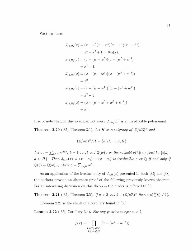
11

We then have:

J12,H1(x) = (x− w)(x− w5)(x− w7)(x− w11)

= x4 − x2 + 1 = Φ12(x).

J12,H2(x) = (x− (w + w5))(x− (w7 + w11)

= x2 + 1.

J12,H3(x) = (x− (w + w7))(x− (w5 + w11))

= x2.

J12,H4(x) = (x− (w + w11))(x− (w5 + w7))

= x2 − 3.

J12,H5(x) = (x− (w + w5 + w7 + w11))

= x.

It is of note that, in this example, not every Jn,Hj(x) is an irreducible polynomial.

Theorem 2.20 ([35], Theorem 3.1). Let H be a subgroup of (Z/nZ)× and

(Z/nZ)×/H = {h1H, . . . , hlH}.

Let ak =∑

h∈H whkh, k = 1, . . . , l and Q(w)H be the subfield of Q(w) fixed by {θ[h] :h ∈ H}. Then Jn,H(x) = (x − a1) · · · (x − al) is irreducible over Q if and only if

Q(ζ) = Q(w)H , where ζ =∑

h∈H wh.

As an application of the irreducibility of Jn,H(x) presented in both [35] and [38],

the authors provide an alternate proof of the following previously known theorem.

For an interesting discussion on this theorem the reader is referred to [8].

Theorem 2.21 ([35], Theorem 3.5). If n > 2 and k ∈ (Z/nZ)× then cos(2πnk) ∈ Q.

Theorem 2.21 is the result of a corollary found in [35]:

Lemma 2.22 ([35], Corollary 3.4). For any positive integer n > 2,

p(x) =∏

k∈(Z/nZ)×,k≤φ(n)/2.

(x− (wk − w−k))

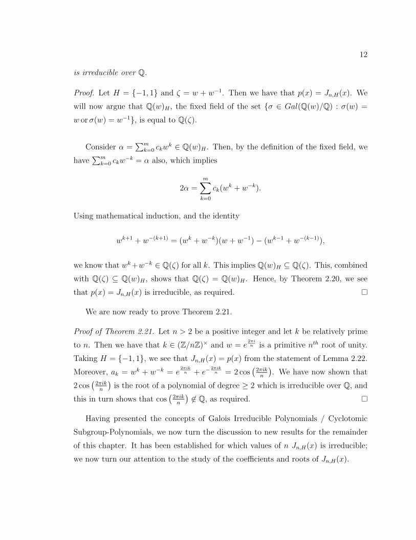
12

is irreducible over Q.

Proof. Let H = {−1, 1} and ζ = w + w−1. Then we have that p(x) = Jn,H(x). We

will now argue that Q(w)H , the fixed field of the set {σ ∈ Gal(Q(w)/Q) : σ(w) =

w orσ(w) = w−1}, is equal to Q(ζ).

Consider α =∑m

k=0 ckwk ∈ Q(w)H . Then, by the definition of the fixed field, we

have∑m

k=0 ckw−k = α also, which implies

2α =m∑k=0

ck(wk + w−k).

Using mathematical induction, and the identity

wk+1 + w−(k+1) = (wk + w−k)(w + w−1)− (wk−1 + w−(k−1)),

we know that wk+w−k ∈ Q(ζ) for all k. This implies Q(w)H ⊆ Q(ζ). This, combined

with Q(ζ) ⊆ Q(w)H , shows that Q(ζ) = Q(w)H . Hence, by Theorem 2.20, we see

that p(x) = Jn,H(x) is irreducible, as required.

We are now ready to prove Theorem 2.21.

Proof of Theorem 2.21. Let n > 2 be a positive integer and let k be relatively prime

to n. Then we have that k ∈ (Z/nZ)× and w = e2πin is a primitive nth root of unity.

Taking H = {−1, 1}, we see that Jn,H(x) = p(x) from the statement of Lemma 2.22.

Moreover, ak = wk + w−k = e2πikn + e−

2πikn = 2 cos

(2πikn

). We have now shown that

2 cos(2πikn

)is the root of a polynomial of degree ≥ 2 which is irreducible over Q, and

this in turn shows that cos(2πikn

)∈ Q, as required.

Having presented the concepts of Galois Irreducible Polynomials / Cyclotomic

Subgroup-Polynomials, we now turn the discussion to new results for the remainder

of this chapter. It has been established for which values of n Jn,H(x) is irreducible;

we now turn our attention to the study of the coefficients and roots of Jn,H(x).

13

2.5 Cases of Interest

To help focus our efforts, we will restrict the values of n to consider. Of special in-

terest to us will be the study of the Cyclotomic Subgroup-Polynomials corresponding

to those integers n for which G = (Z/nZ)× is a cyclic group. Since this choice means

that there exists a unique subgroup H ≤ G of order |H| = d for each d | |G|, wehave an expectation of the number of polynomials Jn,H(x) and their degrees for each

choice of n. The integers of interest are precisely those having primitive roots, and

so we restrict our attention to numbers of the form n = 2, 4, pα, and 2pα, where α is

a positive integer and p is an odd prime.

Moreover, of particular interest to us will be the cases when n is equal to a prime

that is congruent to 1 modulo 3 and when n is equal to a prime congruent to 1 modulo

4. In these cases, we are guaranteed a subgroup H ≤ G of index three and of index

four, respectively, as well as a cubic Cyclotomic Subgroup-Polynomial and a quartic

Cyclotomic Subgroup-Polynomial, respectively.

2.6 Coefficients

In this section, we will investigate the coefficients of different Cyclotomic Subgroup-

Polynomials. We will consider cases by one of two ways: we either restrict the degree

of the polynomial Jn,H(x) by picking a subgroupH of appropriate index, or we restrict

the order of the subgroup H, itself.

2.6.1 The Case Jp,H(x) Where p is an Odd Prime

We begin by studying the case n = p, for an arbitrary odd prime p, before specializing

to particular congruence classes.

We start this subsection by calculating all of the Cyclotomic Subgroup-Polynomials

for the prime p = 11 in the following example:

14

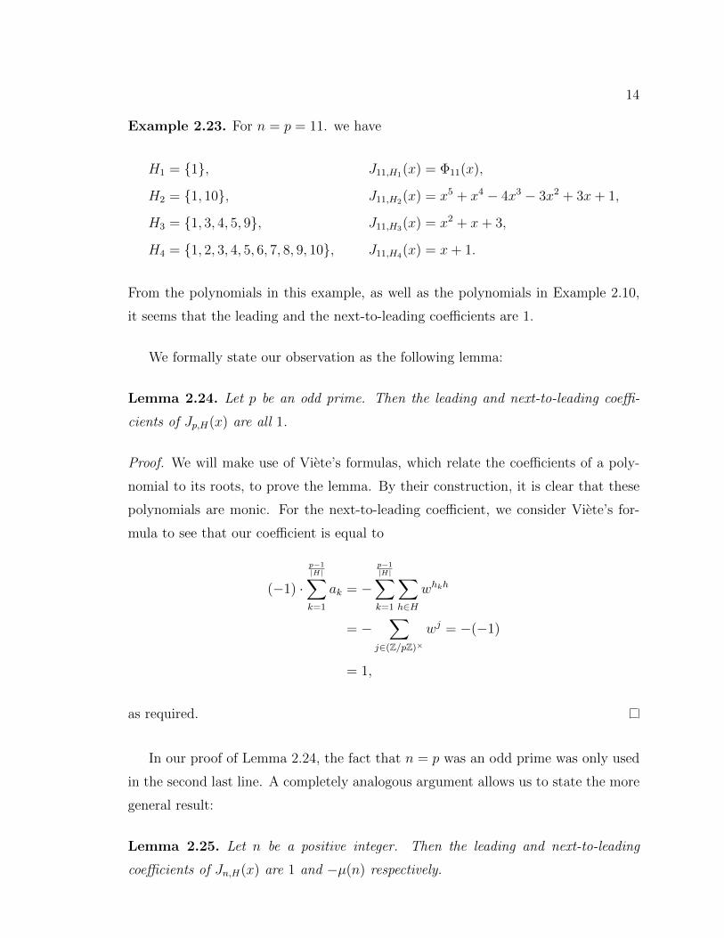
Example 2.23. For n = p = 11. we have

H1 = {1}, J11,H1(x) = Φ11(x),

H2 = {1, 10}, J11,H2(x) = x5 + x4 − 4x3 − 3x2 + 3x+ 1,

H3 = {1, 3, 4, 5, 9}, J11,H3(x) = x2 + x+ 3,

H4 = {1, 2, 3, 4, 5, 6, 7, 8, 9, 10}, J11,H4(x) = x+ 1.

From the polynomials in this example, as well as the polynomials in Example 2.10,

it seems that the leading and the next-to-leading coefficients are 1.

We formally state our observation as the following lemma:

Lemma 2.24. Let p be an odd prime. Then the leading and next-to-leading coeffi-

cients of Jp,H(x) are all 1.

Proof. We will make use of Viete’s formulas, which relate the coefficients of a poly-

nomial to its roots, to prove the lemma. By their construction, it is clear that these

polynomials are monic. For the next-to-leading coefficient, we consider Viete’s for-

mula to see that our coefficient is equal to

(−1) ·p−1|H|∑k=1

ak = −p−1|H|∑k=1

∑h∈H

whkh

= −∑

j∈(Z/pZ)×wj = −(−1)

= 1,

as required.

In our proof of Lemma 2.24, the fact that n = p was an odd prime was only used

in the second last line. A completely analogous argument allows us to state the more

general result:

Lemma 2.25. Let n be a positive integer. Then the leading and next-to-leading

coefficients of Jn,H(x) are 1 and −µ(n) respectively.

15

Proof. The proof of this lemma is analogous to that of Lemma 2.24 except for the

second last equality which is obtained using the identity

∑j∈(Z/nZ)×

wj = µ(n);

see again Theorem A.21 in the appendix.

From Example 2.10 and Example 2.23, as well as more numerical experimentation,

we find the following:

Lemma 2.26. Let Jp,H(x) = xm + xm−1 + bm−2xm−2 + . . .+ b0. Then

bm−2 =

⎧⎨⎩p−12

− |H|2, if |H| is even,

|H|+12

, if |H| is odd.

Proof. Using Viete’s formula, we know that the coefficient of interest is the sum over

all possible 2-products of the roots of Jp,H(x). We begin by calculating the total

number of terms in our “Viete sum”:

N := |H|2 ·(p−1

|H|2

)= |H|2 ·

p−1|H|

(p−1|H| − 1

)2

=(p− 1)(p− 1− |H|)

2.

Case 1 (The index of H is even): Because of the group structure of the quo-

tient group (Z/pZ)× /H ∼= Z/2kZ for an integer k, as well as the group structure of

(Z/pZ)×, we know that we will have no terms that equal 1 in our sum; each element

and its inverse are in the same coset. All of the terms will be in groups of (p − 1)

terms that equal −1, namely (w + w2 + . . .+ wp−1). Therefore,

bm−2 =N

(p− 1)=

p− 1− |H|2

=p− 1

2− |H|

2,

as required.

Case 2 (The index of H is odd): Because of the group structure of the quotient

group (Z/pZ)× /H ∼= Z/(2k + 1)Z for an integer k, as well as the group structure

of (Z/pZ)×, we know that we will have p−12

terms that equal 1 in our sum; each

16

element and its inverse are in different cosets and will be multiplied together. The

remainder of the terms will be in groups of (p− 1) that once again equal −1, namely

(w + w2 + . . .+ wp−1). Therefore,

bm−2 =p− 1

2− N − p−1

2

p− 1=

|H|+ 1

2,

as required.

2.6.2 The Case Jp,{1,−1}(x)

We now turn our attention to subgroups H ≤ (Z/pZ)× of order 2, where p is an

odd prime. This is a particular case of interest because not only does every group

(Z/pZ)× have a subgroup H of order 2, but we also know the two elements in H for

all p. Since p is an odd prime, we know that |(Z/pZ)×| = p − 1 will be even. Then

we have a cyclic group of even order, which must have a unique subgroup of order 2,

namely H = {−1, 1}. The polynomials Jp,{−1,1}(x) are the focus of this subsection.

We begin our discussion by listing the first few examples of these polynomials.

Example 2.27. The polynomials Jp,{−1,1}(x) for the primes p = 3, 5, 7, 11, 13, and 17

are as follows:

J3,{−1,1}(x) = x+ 1,

J5,{−1,1}(x) = x2 + x− 1,

J7,{−1,1}(x) = x3 + x2 − 2x− 1,

J11,{−1,1}(x) = x5 + x4 − 4x3 − 3x2 + 3x+ 1,

J13,{−1,1}(x) = x6 + x5 − 5x4 − 4x3 + 6x2 + 3x− 1,

J17,{−1,1}(x) = x8 + x7 − 7x6 − 6x5 + 15x4 + 10x3 − 10x2 − 4x+ 1.

As seen in Example 2.27, we notice an interesting pattern when considering these

polynomials for various primes p; their coefficients follow a “ladder” pattern in Pas-

cal’s triangle. The pattern depends on the congruence class of p modulo 4 as formal-

ized below:

(a) If p ≡ 1 (mod 4), then the coefficients follow the pattern

17( p−120

);( p−1

2−1

0

),( p−1

2−1

1

);( p−1

2−2

1

),( p−1

2−2

2

);( p−1

2−3

2

),( p−1

2−3

3

); . . . ;

( p−14

p−14

−1

),( p−1

4p−14

).

(b) If p ≡ 3 (mod 4), then the coefficients follow the pattern( p−120

);( p−1

2−1

0

),( p−1

2−1

1

);( p−1

2−2

1

),( p−1

2−2

2

);( p−1

2−3

2

),( p−1

2−3

3

); . . . ;

(⌊ p−14

⌋⌊ p−1

4⌋

).

If we split the odd-degree polynomials from the even-degree polynomials, a con-

nection with the Chebyshev polynomials becomes evident. Some basic properties of

the Chebyshev polynomials are summarized in the Appendix.

Theorem 2.28. For any prime p > 2, we have

Jp,{1,−1}(x) =

p−12∏

k=1

(x− 2 cos

(2πkp

))= Up−1

2

(x2

)+ Up−1

2−1

(x2

)=

(−1)p−12√

12− x

4

Tp

(√12− x

4

),

where Tn(x) denotes the nth Chebyshev polynomial of the first kind and Un(x) denotes

the nth Chebyshev polynomial of the second kind.

Proof. We have

(−1)p−12√

12− x

4

Tp

(√12− x

4

)=

(−1)p−12

2(√

12− x

4

) (Up

(√12− x

4

)− Up−2

(√12− x

4

))

=(−1)

p−12

2(√

12− x

4

)Up

(√12− x

4

)+

(−1)p−12

2(√

12− x

4

)Up−2

(√12− x

4

)

= U p−12

(x2

)+ U p−1

2−1

(x2

),

where we have applied both parts of Lemma A.7 to get the first and last equalities.

18

Now, knowing the roots of Tn(x) explicitly, we can write

(−1)p−12√

12− x

4

Tp

(√12− x

4

)=

(−1)p−12√

12− x

4

p∏k=1

(√12− x

4− cos

(2k−14n+2

π))

= (−1)p−12

p−12∏

k=1

(√12− x

4− cos

(2k−12p

π))

p∏k= p−1

2+2

(√12− x

4− cos

(2k−12p

π))

.

To complete the proof, we need to observe two things. First, the transformations

x → x2→√

12− x

4have doubled the number of roots (the original roots of Tn(x) and

their negatives). Second, the identity cos(θ) = − cos(θ + π) needs to be applied p

times, once for each root, which eliminates the extra factor of (−1)p−12 found above

and will leave us the desired roots and their negatives, as required.

Remark: In this proof, all instances of√

12− x

4could have been replaced with

−√

12− x

4as well.

We conclude this subsection with a corollary of Theorem 2.28. To prove this

corollary, we will require the following identity from [27].

Lemma 2.29 ([27], Identity 91.2.9, pg. 499). When n is an odd integer, we have

n−12∏

k=1

[cos(y)− cos

(2πkn

)]= 2

1−n2 sin

(ny2

)csc(y2

).

A more complete form of this lemma will be given in Section 2.11.

Corollary 2.30. For any prime p > 2, the constant coefficient of Jp,{−1,1}(x) is ±1.

Furthermore, the sign may be determined by the congruence class of p modulo 8.

Namely, if p ≡ 1, 3 (mod 8) then the constant coefficient will be 1 and if p ≡ 5, 7

(mod 8) then the constant coefficient will be −1.

19

Proof. From Theorem 2.28, we know that the constant coefficient will be equal to

(−1)p−12∏ p−1

2k=1 2 cos

(2πkp

). Applying Lemma 2.29, we have

(−1)p−12

p−12∏

k=1

2 cos(

2πkp

)= (−1)

p−12 2

p−12

(2

1−p2 sin

(pπ4

)csc(π4

))= (−1)

p−12 sin

(pπ4

)csc(π4

)= ±1.

If we consider pπ4, we see that if p ≡ 1, 3 (mod 8), then the argument of pπ

4lies in

quadrant 1 or quadrant 2, respectively, and (−1)p−12 sin

(pπ4

)csc(π4

)= 1, as required.

Similarly, if p ≡ 5, 7 (mod 8), then the argument of pπ4lies in quadrant 3 or quadrant

4, respectively, and (−1)p−12 sin

(pπ4

)csc(π4

)= −1, as required.

2.6.3 The Case Jp,H(x) When p ≡ 1 (mod 3) and |H| = 3

In this subsection, we will study another subset of the Cyclotomic Subgroup-Polynomials

Jp,H(x). We focus on primes p ≡ 1 (mod 3) and the subgroup H ≤ (Z/pZ)× of order

3. We begin by listing the first few such examples.

Example 2.31.

J7,{1,2,4}(x) = x2 + x+ 2,

J13,{1,3,9}(x) = x4 + x3 + 2x2 − 4x+ 3,

J19,{1,7,11}(x) = x6 + x5 + 2x4 − 8x3 − x2 + 5x+ 7,

J31,{1,5,25}(x) = x10 + x9 + 2x8 − 16x7 − 9x6 − 11x5 + 43x4 + 6x3 + 63x2 + 20x+ 25.

Lemma 2.32. Let p ≡ 1 (mod 3) and |H| = 3, and write Jp,H(x) = xm + xm−1 +

bm−2xm−2 + . . .+ b0. Then bm−2 = 2.

Proof. This is a direct corollary of Lemma 2.26. However, to illuminate the proof

through the use of a specific example, we present the following stand-alone proof.

Using Viete’s formula, we know that the coefficient in question is the sum over

all possible 2-products of the roots of Jp,H(x). Because we know that |H| = 3, the

total number of terms in the sum is 9 ·( p−1

32

). Because of the group structure of the

20

quotient group (Z/pZ)× /H and the group structure of the group Z/pZ×, we know

that we will have p−12

products that equal 1, namely (wn · wp−n) for n = 1, . . . , p−12.

The remaining terms can then be organized in groups of (p−1) summands that equal

−1, namely (w + w2 + . . .+ wp−1) = −1. Putting all of this together, we get

bm−2 =p− 1

2− 9 ·

( p−132

)− p−1

2

p− 1=

p− 1

2− p− 5

2= 2.

Thus we have shown that bm−2 = 2, as required.

Conjecture 2.33. Let p ≡ 1 (mod 3) and |H| = 3, and write Jp,H(x) = xm+xm−1+

bm−2xm−2 + . . .+ b0. Then

bm−3 = 2

(p− 1

3

)− 4 =

2p− 14

3.

Through numerical experimentation this conjecture has been verified for all odd

primes p ≡ 1 (mod 3), p < 10000. When attempting to prove this conjecture, the

major obstacle was determining the behaviour of sums of the form

∑i,j,k

gigjgk gi, gj, gk ∈ (Z/pZ)×/H

for a given prime p and subgroup H as in the statement of the conjecture.

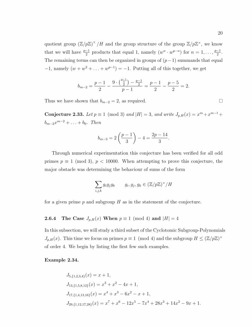
2.6.4 The Case Jp,H(x) When p ≡ 1 (mod 4) and |H| = 4

In this subsection, we will study a third subset of the Cyclotomic Subgroup-Polynomials

Jp,H(x). This time we focus on primes p ≡ 1 (mod 4) and the subgroupH ≤ (Z/pZ)×

of order 4. We begin by listing the first few such examples.

Example 2.34.

J5,{1,2,3,4}(x) = x+ 1,

J13,{1,5,8,12}(x) = x3 + x2 − 4x+ 1,

J17,{1,4,13,16}(x) = x4 + x3 − 6x2 − x+ 1,

J29,{1,12,17,28}(x) = x7 + x6 − 12x5 − 7x4 + 28x3 + 14x2 − 9x+ 1.

21

Lemma 2.35. Let p ≡ 1 (mod 4) and |H| = 4. Then the constant coefficient of

Jp,H(x) is equal to 1.

Proof. Since p ≡ 1 (mod 4), we know that each root of Jp,H(x) in this case is of the

form

ak = wg1k + wg2k + wg3k + wg4k

for k = 1, 2, . . . , p−14. Because H ∼= Z/4Z, we know that g1k = −g4k and g2k = −g3k

for each value of k; this means that every element of (Z/pZ)× is inside the same

coset as its inverse. The constant coefficient is the product of all of the ak and since

each wgik is in the same coset as w−gik there will be no cancellation in the product

defining ak and every element of (Z/pZ) will appear an equal number of times as an

exponent of w. The wgik will cancel each other out in groups of p elements because

w+w2+ . . .+wp−1 = −1 and w0 = 1. Since the total number of terms in the product∏ p−14

k=1 ak will be 4p−14 , we look to write this quantity in the form A · p+B for integers

A and B:

4p−14 = 2

p−12 =

1

p

(2

p−12 −

(2

p

))· p+

(2

p

).

This means that the product of the roots of Jp,H(x) is equal to the Legendre symbol(2p

). Using Viete’s formula, the constant coefficient is equal to (−1)n

(2p

)= 1, as

required.

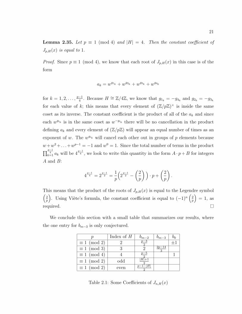
We conclude this section with a small table that summarizes our results, where

the one entry for bm−3 is only conjectured.

p Index of H bm−2 bm−3 b0≡ 1 (mod 2) 2 p−3

2±1

≡ 1 (mod 3) 3 2 2p−143

≡ 1 (mod 4) 4 p−52

1

≡ 1 (mod 2) odd |H|+12

≡ 1 (mod 2) even p−1−|H|2

Table 2.1: Some Coefficients of Jn,H(x)

22

2.7 Studying the Sets {Jn,H(x) |H ≤ (Z/nZ)×}

In this section, we investigate the relationship between sets of Cyclotomic Subgroup-

Polynomials {Jn1,H(x) |H ≤ (Z/n1Z)×} and {Jn2,H(x) |H ≤ (Z/n2Z)×} for different

positive integers n1 and n2.

2.7.1 The Case n1 = p Compared to the Case n2 = 2p

We first consider the case with n1 = p an odd prime and n2 = 2p. In this case,

(Z/pZ)× and (Z/2pZ)× are both cyclic, and φ(n1) = φ(n2) = p−1. So we know that

the two sets will be of equal cardinality, i.e., contain the same number of polynomials

with the same degrees. We calculate such an example with n1 = 7 and n2 = 14:

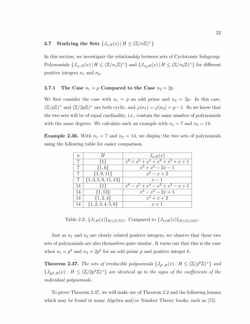
Example 2.36. With n1 = 7 and n2 = 14, we display the two sets of polynomials

using the following table for easier comparison.

n H Jn,H(x)7 {1} x6 + x5 + x4 + x3 + x2 + x+ 17 {1, 6} x3 + x2 − 2x− 17 {1, 9, 11} x2 − x+ 27 {1, 3, 5, 9, 11, 13} x− 114 {1} x6 − x5 + x4 − x3 + x2 − x+ 114 {1, 13} x3 − x2 − 2x+ 114 {1, 2, 4} x2 + x+ 214 {1, 2, 3, 4, 5, 6} x+ 1

Table 2.2: {J7,H(x)}H≤(Z/7Z)× Compared to {J14,H(x)}H≤(Z/14Z)×

Just as n1 and n2 are closely related positive integers, we observe that these two

sets of polynomials are also themselves quite similar. It turns out that this is the case

when n1 = pk and n2 = 2pk for an odd prime p and positive integer k.

Theorem 2.37. The sets of irreducible polynomials {Jpk,H(x) : H ≤ (Z/pkZ)×} and

{J2pk,H(x) : H ≤ (Z/2pkZ)×} are identical up to the signs of the coefficients of the

individual polynomials.

To prove Theorem 2.37, we will make use of Theorem 2.2 and the following lemma

which may be found in many Algebra and/or Number Theory books, such as [15]:

23

Lemma 2.38 ([15], Lemma 1.4.5). Let p be an odd prime, and let g be a primitive

root modulo pk. Then either g or (g+pk) (whichever is odd) is a primitive root modulo

2pk for all positive integers k.

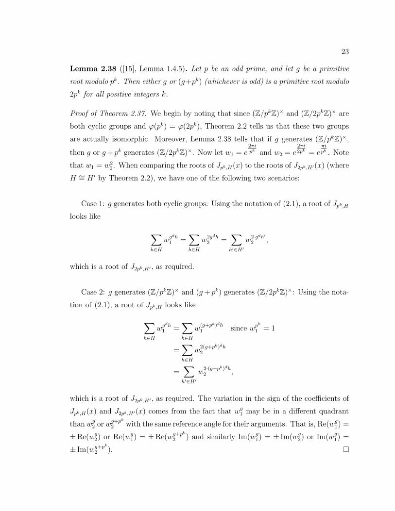
Proof of Theorem 2.37. We begin by noting that since (Z/pkZ)× and (Z/2pkZ)× are

both cyclic groups and φ(pk) = φ(2pk), Theorem 2.2 tells us that these two groups

are actually isomorphic. Moreover, Lemma 2.38 tells that if g generates (Z/pkZ)×,

then g or g+ pk generates (Z/2pkZ)×. Now let w1 = e2πipk and w2 = e

2πi2pk = e

πipk . Note

that w1 = w22. When comparing the roots of Jpk,H(x) to the roots of J2pk,H′(x) (where

H ∼= H ′ by Theorem 2.2), we have one of the following two scenarios:

Case 1: g generates both cyclic groups: Using the notation of (2.1), a root of Jpk,H

looks like

∑h∈H

wgdh1 =

∑h∈H

w2gdh2 =

∑h′∈H′

w2·gdh′

2 ,

which is a root of J2pk,H′ , as required.

Case 2: g generates (Z/pkZ)× and (g+ pk) generates (Z/2pkZ)×: Using the nota-

tion of (2.1), a root of Jpk,H looks like

∑h∈H

wgdh1 =

∑h∈H

w(g+pk)dh1 since wpk

1 = 1

=∑h∈H

w2(g+pk)dh2

=∑h′∈H′

w2·(g+pk)dh2 ,

which is a root of J2pk,H′ , as required. The variation in the sign of the coefficients of

Jpk,H(x) and J2pk,H′(x) comes from the fact that wg1 may be in a different quadrant

than wg2 or w

g+pk

2 with the same reference angle for their arguments. That is, Re(wg1) =

±Re(wg2) or Re(wg

1) = ±Re(wg+pk

2 ) and similarly Im(wg1) = ± Im(wg

2) or Im(wg1) =

± Im(wg+pk

2 ).

24

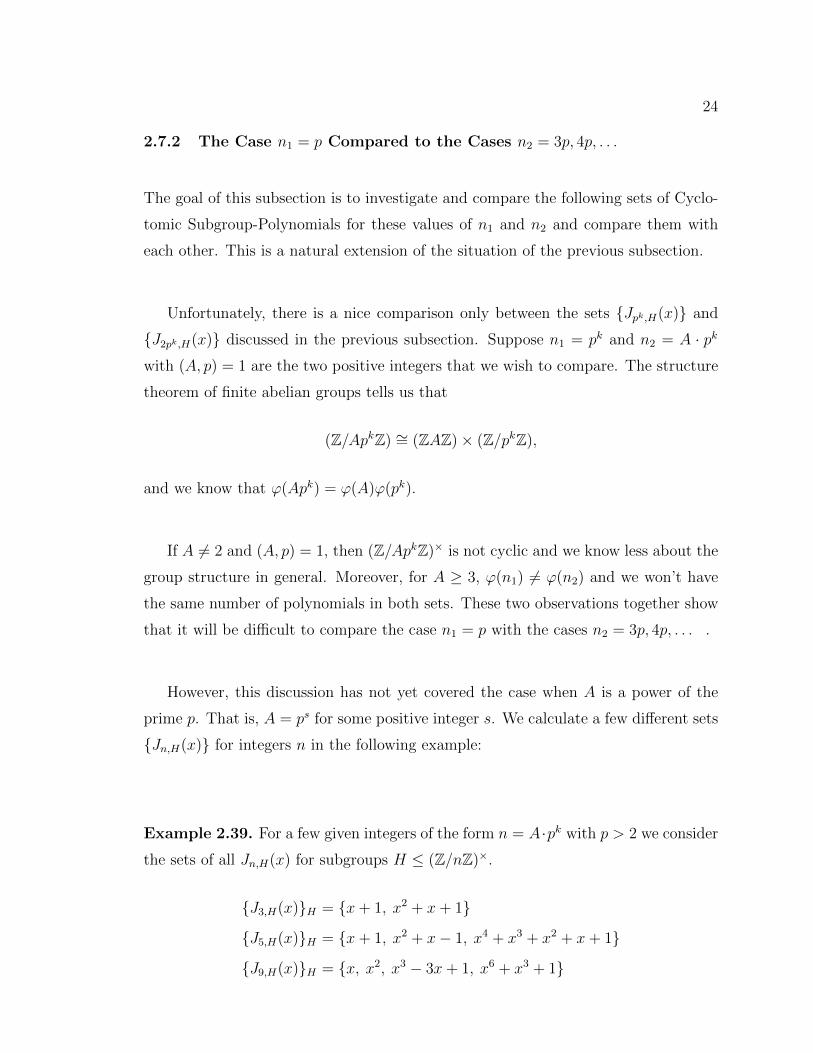
2.7.2 The Case n1 = p Compared to the Cases n2 = 3p, 4p, . . .

The goal of this subsection is to investigate and compare the following sets of Cyclo-

tomic Subgroup-Polynomials for these values of n1 and n2 and compare them with

each other. This is a natural extension of the situation of the previous subsection.

Unfortunately, there is a nice comparison only between the sets {Jpk,H(x)} and

{J2pk,H(x)} discussed in the previous subsection. Suppose n1 = pk and n2 = A · pk

with (A, p) = 1 are the two positive integers that we wish to compare. The structure

theorem of finite abelian groups tells us that

(Z/ApkZ) ∼= (ZAZ)× (Z/pkZ),

and we know that φ(Apk) = φ(A)φ(pk).

If A = 2 and (A, p) = 1, then (Z/ApkZ)× is not cyclic and we know less about the

group structure in general. Moreover, for A ≥ 3, φ(n1) = φ(n2) and we won’t have

the same number of polynomials in both sets. These two observations together show

that it will be difficult to compare the case n1 = p with the cases n2 = 3p, 4p, . . . .

However, this discussion has not yet covered the case when A is a power of the

prime p. That is, A = ps for some positive integer s. We calculate a few different sets

{Jn,H(x)} for integers n in the following example:

Example 2.39. For a few given integers of the form n = A·pk with p > 2 we consider

the sets of all Jn,H(x) for subgroups H ≤ (Z/nZ)×.

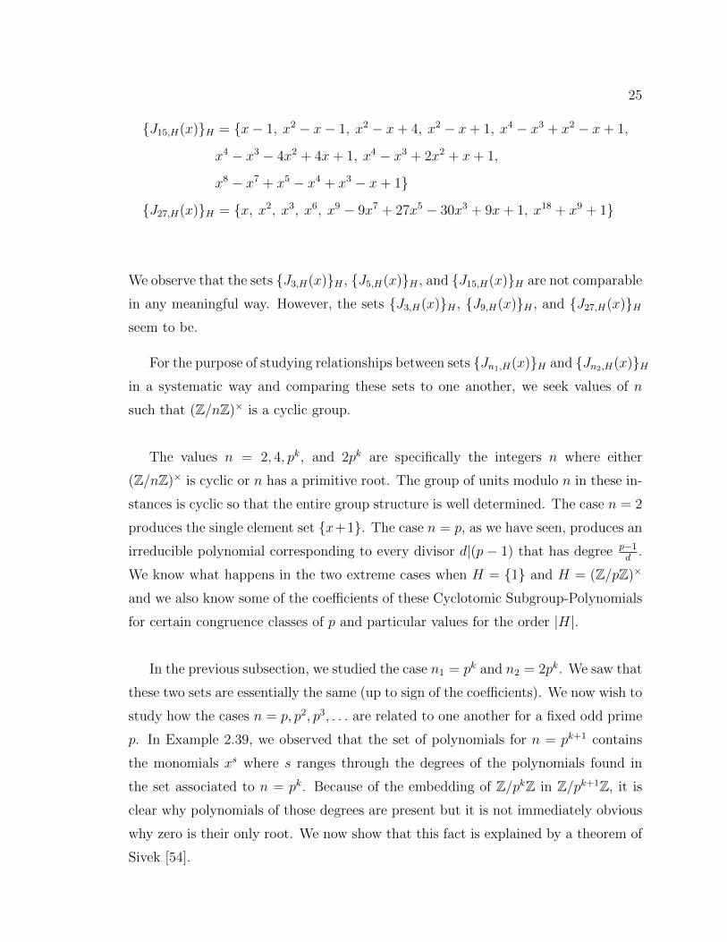
{J3,H(x)}H = {x+ 1, x2 + x+ 1}{J5,H(x)}H = {x+ 1, x2 + x− 1, x4 + x3 + x2 + x+ 1}{J9,H(x)}H = {x, x2, x3 − 3x+ 1, x6 + x3 + 1}

25

{J15,H(x)}H = {x− 1, x2 − x− 1, x2 − x+ 4, x2 − x+ 1, x4 − x3 + x2 − x+ 1,

x4 − x3 − 4x2 + 4x+ 1, x4 − x3 + 2x2 + x+ 1,

x8 − x7 + x5 − x4 + x3 − x+ 1}{J27,H(x)}H = {x, x2, x3, x6, x9 − 9x7 + 27x5 − 30x3 + 9x+ 1, x18 + x9 + 1}

We observe that the sets {J3,H(x)}H , {J5,H(x)}H , and {J15,H(x)}H are not comparable

in any meaningful way. However, the sets {J3,H(x)}H , {J9,H(x)}H , and {J27,H(x)}Hseem to be.

For the purpose of studying relationships between sets {Jn1,H(x)}H and {Jn2,H(x)}Hin a systematic way and comparing these sets to one another, we seek values of n

such that (Z/nZ)× is a cyclic group.

The values n = 2, 4, pk, and 2pk are specifically the integers n where either

(Z/nZ)× is cyclic or n has a primitive root. The group of units modulo n in these in-

stances is cyclic so that the entire group structure is well determined. The case n = 2

produces the single element set {x+1}. The case n = p, as we have seen, produces an

irreducible polynomial corresponding to every divisor d|(p − 1) that has degree p−1d.

We know what happens in the two extreme cases when H = {1} and H = (Z/pZ)×

and we also know some of the coefficients of these Cyclotomic Subgroup-Polynomials

for certain congruence classes of p and particular values for the order |H|.

In the previous subsection, we studied the case n1 = pk and n2 = 2pk. We saw that

these two sets are essentially the same (up to sign of the coefficients). We now wish to

study how the cases n = p, p2, p3, . . . are related to one another for a fixed odd prime

p. In Example 2.39, we observed that the set of polynomials for n = pk+1 contains

the monomials xs where s ranges through the degrees of the polynomials found in

the set associated to n = pk. Because of the embedding of Z/pkZ in Z/pk+1Z, it isclear why polynomials of those degrees are present but it is not immediately obvious

why zero is their only root. We now show that this fact is explained by a theorem of

Sivek [54].

26

2.8 Vanishing Roots of Unity

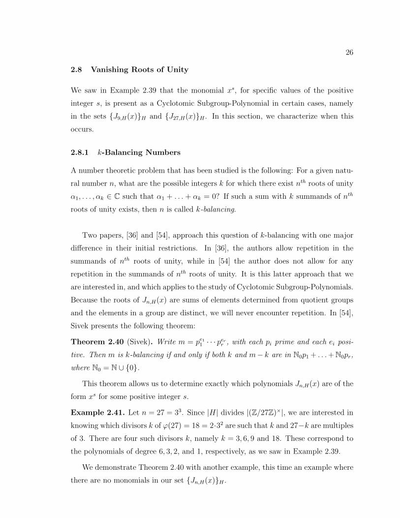
We saw in Example 2.39 that the monomial xs, for specific values of the positive

integer s, is present as a Cyclotomic Subgroup-Polynomial in certain cases, namely

in the sets {J9,H(x)}H and {J27,H(x)}H . In this section, we characterize when this

occurs.

2.8.1 k-Balancing Numbers

A number theoretic problem that has been studied is the following: For a given natu-

ral number n, what are the possible integers k for which there exist nth roots of unity

α1, . . . , αk ∈ C such that α1 + . . . + αk = 0? If such a sum with k summands of nth

roots of unity exists, then n is called k-balancing.

Two papers, [36] and [54], approach this question of k-balancing with one major

difference in their initial restrictions. In [36], the authors allow repetition in the

summands of nth roots of unity, while in [54] the author does not allow for any

repetition in the summands of nth roots of unity. It is this latter approach that we

are interested in, and which applies to the study of Cyclotomic Subgroup-Polynomials.

Because the roots of Jn,H(x) are sums of elements determined from quotient groups

and the elements in a group are distinct, we will never encounter repetition. In [54],

Sivek presents the following theorem:

Theorem 2.40 (Sivek). Write m = pe11 · · · perr , with each pi prime and each ei posi-

tive. Then m is k-balancing if and only if both k and m− k are in N0p1 + . . .+N0pr,

where N0 = N ∪ {0}.

This theorem allows us to determine exactly which polynomials Jn,H(x) are of the

form xs for some positive integer s.

Example 2.41. Let n = 27 = 33. Since |H| divides |(Z/27Z)×|, we are interested in

knowing which divisors k of φ(27) = 18 = 2·32 are such that k and 27−k are multiples

of 3. There are four such divisors k, namely k = 3, 6, 9 and 18. These correspond to

the polynomials of degree 6, 3, 2, and 1, respectively, as we saw in Example 2.39.

We demonstrate Theorem 2.40 with another example, this time an example where

there are no monomials in our set {Jn,H(x)}H .

27

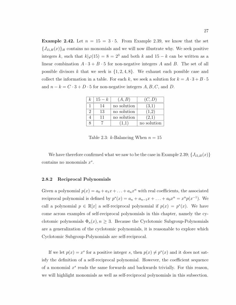
Example 2.42. Let n = 15 = 3 · 5. From Example 2.39, we know that the set

{J15,H(x)}H contains no monomials and we will now illustrate why. We seek positive

integers k, such that k|φ(15) = 8 = 23 and both k and 15 − k can be written as a

linear combination A · 3 + B · 5 for non-negative integers A and B. The set of all

possible divisors k that we seek is {1, 2, 4, 8}. We exhaust each possible case and

collect the information in a table. For each k, we seek a solution for k = A · 3 +B · 5and n− k = C · 3 +D · 5 for non-negative integers A,B,C, and D.

k 15− k (A,B) (C,D)

1 14 no solution (3,1)2 13 no solution (1,2)4 11 no solution (2,1)8 7 (1,1) no solution

Table 2.3: k-Balancing When n = 15

We have therefore confirmed what we saw to be the case in Example 2.39; {J15,H(x)}contains no monomials xs.

2.8.2 Reciprocal Polynomials

Given a polynomial p(x) = a0+ a1x+ . . .+ anxn with real coefficients, the associated

reciprocal polynomial is defined by p∗(x) = an + an−1x+ . . .+ a0xn = xnp(x−1). We

call a polynomial p ∈ R[x] a self-reciprocal polynomial if p(x) = p∗(x). We have

come across examples of self-reciprocal polynomials in this chapter, namely the cy-

clotomic polynomials Φn(x), n ≥ 3. Because the Cyclotomic Subgroup-Polynomials

are a generalization of the cyclotomic polynomials, it is reasonable to explore which

Cyclotomic Subgroup-Polynomials are self-reciprocal.

If we let p(x) = xs for a positive integer s, then p(x) = p∗(x) and it does not sat-

isfy the definition of a self-reciprocal polynomial. However, the coefficient sequence

of a monomial xs reads the same forwards and backwards trivially. For this reason,

we will highlight monomials as well as self-reciprocal polynomials in this subsection.

28

In [12], Cafure and Cesaratto give a useful characterization of self-reciprocal poly-

nomials in terms of their roots.

Theorem 2.43 (Cafure and Cesaratto). A polynomial f ∈ Q[x] is self-reciprocal if

and only if it satisfies the following two properties:

If 1 is a root of f , then its multiplicity is even.

If α is a root of f of multiplicity r, then 1αis a root of multiplicity r.

This characterization, based on the roots of a self-reciprocal polynomial, proves

to be the most useful characterization when discussing the Cyclotomic Subgroup-

Polynomials Jn,H(x) since they are generated by first calculating their roots. Theo-

rem 2.43 allows us to state and prove the following result.

Every family of Cyclotomic Subgroup-Polynomials contains the self-reciprocal

polynomial Jn,{1}(x) = Φn(x). In certain cases, depending on the prime decomposi-

tion of n, we can enumerate the exact number of self-reciprocal polynomials and/or

monomials found in the set {Jn,H(x)}H .

Theorem 2.44. (i) When n = p, we have the unique additional self-reciprocal poly-

nomial Jp,(Z/pZ)×(x) = x+ 1.

(ii) When n = pα, α > 1, we have the additional [d(p − 1) · (α − 1)] monomials,

where d(p− 1) is the number of divisors of (p− 1), and there are are no more.

(iii) When n = p1 · p2 · · · pk, we have an additional 2k − 2 self-reciprocal polynomials

for a total of exactly (2k − 1) self-reciprocal polynomials, and there are no more.

Proof. We begin by making a general remark regarding the conditions of Theorem

2.43. From (2.1), we see that the roots of the Cyclotomic Subgroup-Polynomials will

never be equal to 1 and therefore vacuously satisfy the condition that 1 is a root of

even multiplicity. Also from (2.1), we see that for ak and 1ak

to both be roots of the

polynomial, ak will need to itself be a root of unity since∑

h∈H whkh and 1∑h∈H whkh

would both have to be of the form ak′ =∑

h∈H wh′kh for some k

′. If ak is a root of

unity for some k, then every ak is a root of unity since they are all defined in terms

of coset representatives of the subgroup H. We now prove the theorem by addressing

29

each case individually and in order.

Let n = p and let H = (Z/pZ)×. From (2.1) we then have a1 =∑p−1

j=1 wj = −1

and from (2.2), we get Jp,(Z/pZ)×(x) = x + 1 as stated. To show that we do not

have any other self-reciprocal polynomials we use Theorem 2.43, and the fundamen-

tal theorem of finite abelian groups that tells us there is no subgroup H ≤ (Z/pZ)×

such that H ∼= (Z/mZ)× for some integer m since p has no non-trivial proper divisors.

Now let n = pα, α > 1. We will use Theorem 2.40 to help resolve this case.

Since φ(n) = φ(pα) = pα−1(p − 1), we see that if k is a divisor of φ(n), then

k = 1, p, p2, . . . , pα−1 or k|(p − 1) and all possible products are from both of these

sets. We then seek the cases where k and n − k are both multiples of p. We see

that this eliminates k = 1. The divisors k = p, p2, . . . , pα−1 all satisfy the condi-

tions of Theorem 2.40 and correspond to (α − 1) different monomials in our set of

Cyclotomic Subgroup-Polynomials. For any divisor s|(p − 1), s = 1, the product

k = sp, sp2, . . . , spα−1 also satisfy the conditions of Theorem 2.40. Moreover, the fun-

damental theorem of finite abelian groups tells us that there are no other subgroups

H ≤ (Z/nZ)× such that∑

h∈H whkh would be isomorphic to an mth root of unity for

some integer m since there are no other divisors of n.

Lastly, we now let n = p1 · p2 · · · pk. The fundamental theorem of finite abelian

groups tells us that

(Z/nZ)× ∼= (Z/p1Z)× × (Z/p2Z)× × · · · × (Z/pkZ)×.

We can quotient the group (Z/nZ)× by any combination of the subgroups (Z/pjZ)×

and the resulting quotient group will be isomorphic to the group of roots of unity of

order n/∏

j pj. There are 2k total combinations of these pj, and we exclude the two

extreme cases corresponding to choosing none of the pj and choosing all of the pj.

This gives us the required (2k − 2) self-reciprocal polynomials we seek.

We have exhausted all three cases and thus have proved the theorem.

30

We now conclude this section with three examples.

Example 2.45. Recall that in the case n = 7, by Example 2.10, we have a total of

2 self-reciprocal polynomials.

{J7,H(x)} = {x+ 1,

x2 + x+ 2,

x3 + x2 − 2x− 1,

x6 + x5 + x4 + x3 + x2 + x+ 1}.

The self-reciprocal polynomials have been underlined for emphasis.

Example 2.46. Recall that in the case n = 15 = 3 · 5, by Example 2.39, we have a

total of 22 − 1 = 3 self-reciprocal polynomials.

{J15,H(x)} = {x− 1,

x2 − x− 1,

x2 − x+ 4,

x2 − x+ 1,

x4 − x3 + x2 − x+ 1,

x4 − x3 − 4x2 + 4x+ 1,

x4 − x3 + 2x2 + x+ 1,

x8 − x7 + x5 − x4 + x3 − x+ 1}.

The self-reciprocal polynomials have again been underlined for emphasis.

Example 2.47. If we take n = 105 = 3 · 5 · 7, then the set {J105,H(x)} will contain

exactly 23 − 1 = 7 self-reciprocal polynomials. The degrees of these self-reciprocal

polynomials will be, in descending order, 48, 24, 12, 8, 6, 4, and 2. Due to its size,

we refrain from listing the entire set of Cyclotomic Subgroup-Polynomials in this

example.

For the integers that do not conform to one of the three specific cases of Theorem

2.44, the values presented in the theorem represent a lower bound. For example, if

31

n = Apα with (A, p) = 1 then we would have at least an additional [d(p− 1) · (α− 1)]

monomials and/or self-reciprocal polynomials.

2.9 Gauss Period Sums

Let Fpα be the finite field with pα elements for an odd prime p and let g be a primitive

root modulo pα, i.e., g generates the cyclic group (Z/pαZ)×. For any divisor d|(p−1),

we write p− 1 = dm; then Barcanescu [6] defines the Gauss d-periods to be

ηj =∑

x∈{gkd+j :k=0,1,...,m−1}

ζx, j = 0, 1, 2, . . . , d− 1,

where ζ is a fixed primitive root of unity of order p. In [47], the author calls these

ηj, “Gauss sums” as a convenient terminology but warns that the term doesn’t agree

with others in the literature.

In certain cases, namely when when α = 1 and we are considering sums over Fp,

these ηj’s are the roots of the Cyclotomic Subgroup-Polynomials, ak from (2.1). In

some cases of small degree, this allows us to calculate the coefficients of some of the

Cyclotomic Subgroup-Polynomials. Specifically these cases occur when n = p is an

odd prime and the polynomial is of degree two, three, and four.

To properly state the results regarding the Gauss Period Sums, we must discuss

the ability to write a prime number as a linear combination of two square integers.

These results, due to Fermat and proven by Euler, can be found, with proof, in [7]

and [17].

Theorem 2.48 (Fermat). (i) An odd prime p can be written as a sum of two in-

teger squares if and only if p ≡ 1 (mod 4).

(ii) An odd prime p can be written as p = x2 + 2y2, where x, y ∈ Z, if and only if

p ≡ 1, 3 (mod 8).

(iii) An odd prime p can be written as p = x2 + 3y2, where x, y ∈ Z, if and only if

p ≡ 2 (mod 3).

32

We note that when we write p = x2+y2, p = x2+2y2, or p = x2+3y2 for integers

x and y, these representations are unique up to the sign of x and y. For proofs of

this, see [48, pp. 167–174], and in particular, Corollary 3.23 and Theorem 3.27 with

d = −12 and d = −8, respectively.

Let p ≡ 1 (mod 3) be prime. By Theorem 2.48 we know that such primes p admit

a representation as a sum of an integer square and 3 times an integer square. But if

we consider such a representation p = x2 + 3y2 for integers x and y modulo 3, and

use the fact that the only squares modulo 3 are 0 and 1, we can conclude that x2 is

congruent to 1 modulo 3. The congruence x2 ≡ 1 (mod 3) then implies that x ≡ ±1

(mod 3). Finally, by switching the sign of x if necessary, we can assume that x ≡ 1

(mod 3). It follows that, with r = 2x, s = 2y we can represent 4p = r2+3s2 with r ≡ 1

(mod 3). The notation that will be used in Theorems 2.52–2.54 therefore makes sense.

When considering the general case given by p = x2+ny2 for integers x and y and

an arbitrary positive integer n one should be careful, the fact that a prime dividing an

integer of this form need not imply that the prime is of the same form. For example,

consider n = 5: 3 | 21 = 12 + 5 · 22 but 3 = x2 + 5y2 for integers x and y.

To completely answer the question of when a prime can be written as p = x2+ny2

for integers x, y and a given positive integer n, is beyond the scope of this thesis, and

we have listed only the results that will be needed for our use. We refer the interested

reader to [17] for a complete and thorough discussion of the subject.

We now list the first few examples of the specific Cyclotomic Subgroup-Polynomials

that will be the focus of this section, grouped by their degrees.

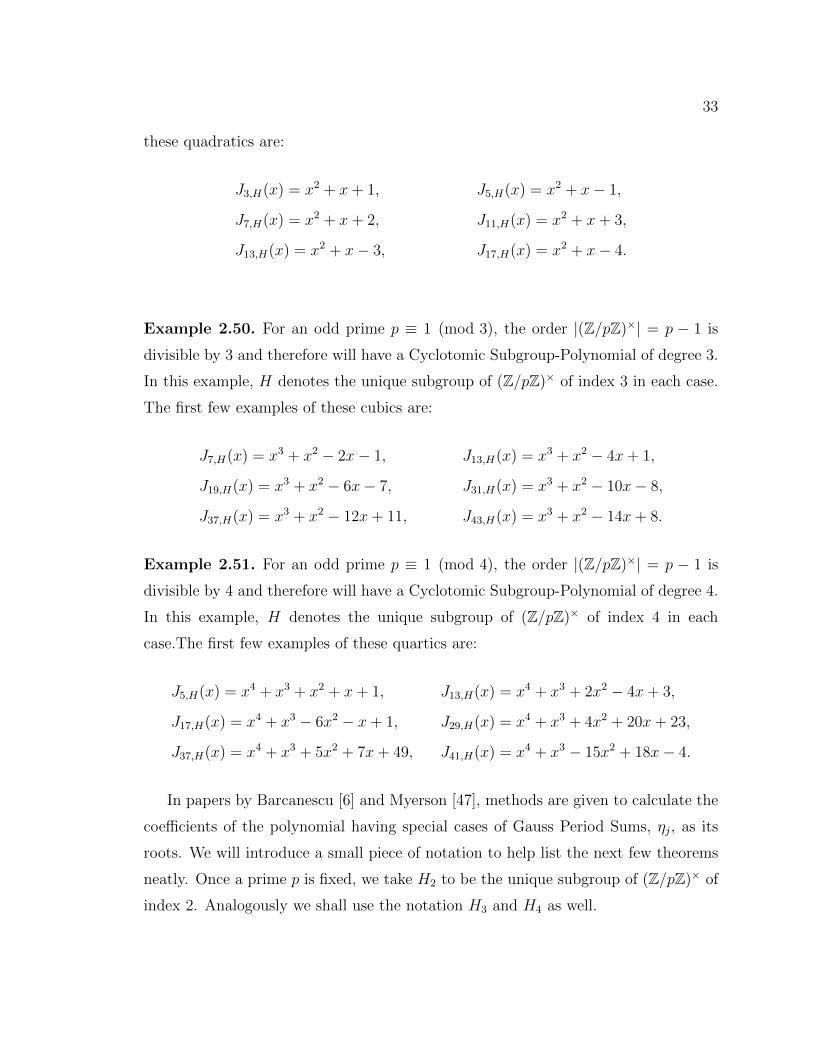
Example 2.49. For an odd prime p, the order |(Z/pZ)×| = p−1 is even and therefore

will have a Cyclotomic Subgroup-Polynomial of degree 2. In this example, H denotes

the unique subgroup of (Z/pZ)× of index 2 in each case. The first few examples of

33

these quadratics are:

J3,H(x) = x2 + x+ 1, J5,H(x) = x2 + x− 1,

J7,H(x) = x2 + x+ 2, J11,H(x) = x2 + x+ 3,

J13,H(x) = x2 + x− 3, J17,H(x) = x2 + x− 4.

Example 2.50. For an odd prime p ≡ 1 (mod 3), the order |(Z/pZ)×| = p − 1 is

divisible by 3 and therefore will have a Cyclotomic Subgroup-Polynomial of degree 3.

In this example, H denotes the unique subgroup of (Z/pZ)× of index 3 in each case.

The first few examples of these cubics are:

J7,H(x) = x3 + x2 − 2x− 1, J13,H(x) = x3 + x2 − 4x+ 1,

J19,H(x) = x3 + x2 − 6x− 7, J31,H(x) = x3 + x2 − 10x− 8,

J37,H(x) = x3 + x2 − 12x+ 11, J43,H(x) = x3 + x2 − 14x+ 8.

Example 2.51. For an odd prime p ≡ 1 (mod 4), the order |(Z/pZ)×| = p − 1 is

divisible by 4 and therefore will have a Cyclotomic Subgroup-Polynomial of degree 4.

In this example, H denotes the unique subgroup of (Z/pZ)× of index 4 in each

case.The first few examples of these quartics are:

J5,H(x) = x4 + x3 + x2 + x+ 1, J13,H(x) = x4 + x3 + 2x2 − 4x+ 3,

J17,H(x) = x4 + x3 − 6x2 − x+ 1, J29,H(x) = x4 + x3 + 4x2 + 20x+ 23,

J37,H(x) = x4 + x3 + 5x2 + 7x+ 49, J41,H(x) = x4 + x3 − 15x2 + 18x− 4.

In papers by Barcanescu [6] and Myerson [47], methods are given to calculate the

coefficients of the polynomial having special cases of Gauss Period Sums, ηj, as its

roots. We will introduce a small piece of notation to help list the next few theorems

neatly. Once a prime p is fixed, we take H2 to be the unique subgroup of (Z/pZ)× of

index 2. Analogously we shall use the notation H3 and H4 as well.

34

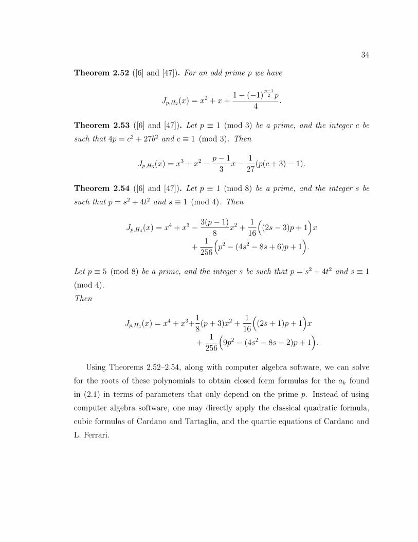
Theorem 2.52 ([6] and [47]). For an odd prime p we have

Jp,H2(x) = x2 + x+1− (−1)

p−12 p

4.

Theorem 2.53 ([6] and [47]). Let p ≡ 1 (mod 3) be a prime, and the integer c be

such that 4p = c2 + 27b2 and c ≡ 1 (mod 3). Then

Jp,H3(x) = x3 + x2 − p− 1

3x− 1

27(p(c+ 3)− 1).

Theorem 2.54 ([6] and [47]). Let p ≡ 1 (mod 8) be a prime, and the integer s be

such that p = s2 + 4t2 and s ≡ 1 (mod 4). Then

Jp,H4(x) = x4 + x3 − 3(p− 1)

8x2 +

1

16

((2s− 3)p+ 1

)x

+1

256

(p2 − (4s2 − 8s+ 6)p+ 1

).

Let p ≡ 5 (mod 8) be a prime, and the integer s be such that p = s2 + 4t2 and s ≡ 1

(mod 4).

Then

Jp,H4(x) = x4 + x3+1

8(p+ 3)x2 +

1

16

((2s+ 1)p+ 1

)x

+1

256

(9p2 − (4s2 − 8s− 2)p+ 1

).

Using Theorems 2.52–2.54, along with computer algebra software, we can solve

for the roots of these polynomials to obtain closed form formulas for the ak found

in (2.1) in terms of parameters that only depend on the prime p. Instead of using

computer algebra software, one may directly apply the classical quadratic formula,

cubic formulas of Cardano and Tartaglia, and the quartic equations of Cardano and

L. Ferrari.

35

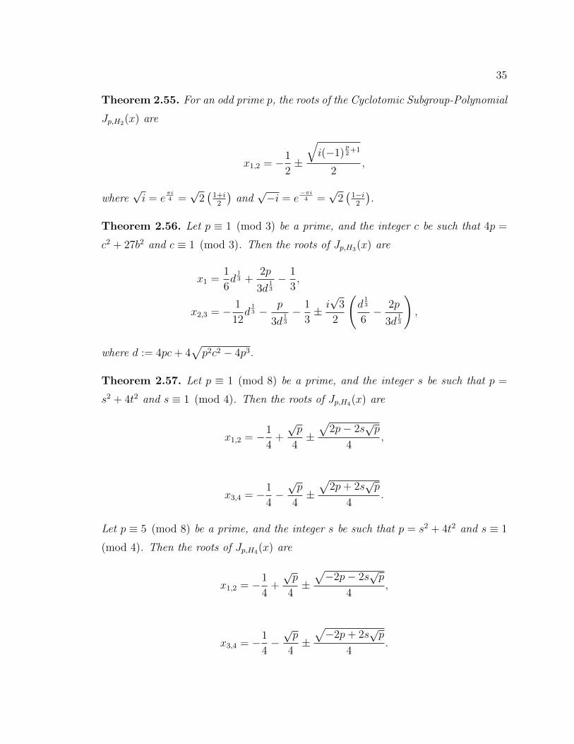
Theorem 2.55. For an odd prime p, the roots of the Cyclotomic Subgroup-Polynomial

Jp,H2(x) are

x1,2 = −1

2±

√i(−1)

p2+1

2,

where√i = e

πi4 =

√2(1+i2

)and

√−i = e

−πi4 =

√2(1−i2

).

Theorem 2.56. Let p ≡ 1 (mod 3) be a prime, and the integer c be such that 4p =

c2 + 27b2 and c ≡ 1 (mod 3). Then the roots of Jp,H3(x) are

x1 =1

6d

13 +

2p

3d13

− 1

3,

x2,3 = − 1

12d

13 − p

3d13

− 1

3± i

√3

2

(d

13

6− 2p

3d13

),

where d := 4pc+ 4√

p2c2 − 4p3.

Theorem 2.57. Let p ≡ 1 (mod 8) be a prime, and the integer s be such that p =

s2 + 4t2 and s ≡ 1 (mod 4). Then the roots of Jp,H4(x) are

x1,2 = −1

4+

√p

4±√

2p− 2s√p

4,

x3,4 = −1

4−

√p

4±√

2p+ 2s√p

4.

Let p ≡ 5 (mod 8) be a prime, and the integer s be such that p = s2 + 4t2 and s ≡ 1

(mod 4). Then the roots of Jp,H4(x) are

x1,2 = −1

4+

√p

4±√

−2p− 2s√p

4,

x3,4 = −1

4−

√p

4±√

−2p+ 2s√p

4.

36

2.10 Integral Formula for the Constant Coefficient of the Cyclotomic

Subgroup-Polynomial

In [1] and [2], Andrica and Bagdasar present the polygonal polynomials, Pn(x), which

they define as follows:

Definition 2.58. For a positive integer n,

Pn(z) = (z − 1)(z2 − 1) · · · (zn − 1).

The polygonal polynomials are a special case of a more general family of polyno-

mials, also introduced in [1] and [2], defined as follows.

Definition 2.59. For positive integers n,m1,m2, . . . ,mn, and complex numbers z1, z2,

. . . , zn which satisfy |zk| = 1 for k = 1, . . . , n, we define

F z1,z2,...,znm1,m2,...,mn

(z) =n∏

k=1

(zmk − zk).

Motivated by the results of Andrica and Bagdasar, in this section we apply the

methodology found in [2] to provide an integral formula for calculating the constant

coefficient of the Cyclotomic Subgroup-Polynomial Jn,H(x).

Theorem 2.60. The constant coefficient b0 of the Cyclotomic Subgroup-Polynomial

Jn,H(x) is given by the integral formula

b0 = |a1| · |a2| · · · |aN |(2i)N

π

∫ π

0

N∏k=1

sin(t− αk

N

)ei(Nt+

α2 )dt,

where N is the degree of Jn,H(x), and α = α1 +α2 + . . .+αN with arg(ak) = αk, and

a1, . . . , aN given by (2.1).

Proof. The proof is based on a combination of two proofs found in [1] and [2]. We

begin by scaling the roots ak found in (2.1) to be on the unit circle. We will account

for this change in the final step of the proof. Set Ak =ak|ak|

. Given equation (2.2), we

want to re-write the difference (x− Ak). We let x = cos(2t) + i sin(2t) for t ∈ [0, π].

37

We then have

x− Ak =(cos(2t)− cos(αk)

)+ i(sin(2t)− sin(αk)

)= −2 sin

(t− αk

2

)sin(t+ αk

2

)+ 2i sin

(t− αk

2

)cos(t+ αk

2

)= 2i sin

(t− αk

2

) (cos(t+ αk

2

)+ i sin

(t+ αk

2

) )= 2i sin

(t− αk

2

)ei(t+

αk

2 ).

We write ˜Jn,H(x) to indicate that we have manipulated the original roots of the

Cyclotomic Subgroup-Polynomial Jn,H(x). Then

˜Jn,H(x) = N∑j=0

cjxj =

N∏k=1

(x− Ak),

= (2i)NN∏k=1

sin(t− αk

2

)· ei(t+

αk

2 ),

= (2i)NN∏k=1

sin(t− αk

2

)· ei(Nt+

α2 ).

Separating the constant coefficient, we now have the following:

c0 +N∑k=1

ckxk =

N∏k=1

(x− Ak),

= (2i)NN∏k=1

sin(t− αk

2

)· ei(Nt+

α2 ),

= (2i)NN∏k=1

sin(t− αk

2

)· ei(Nt+

α2 ).

Since x = cos(2t) + i sin(2t), t ∈ [0, π], we observe that t = 0 and t = π return the

same value for x. Therefore:

∫ π

0

(c0 +

N∑k=1

ckxk

)dt =

∫ π

0

c0 dt+

∫ π

0

n∑k=1

ckxkdt

=

∫ π

0

c0 dt.

38

Then, adjusting for our scaled roots as well as integrating a constant function

over an interval of length π, the constant coefficient of the Cyclotomic Subgroup-

Polynomial Jn,H(x) is

b0 = (|a1| · |a2| · · · |aN |)(2i)N

π

∫ π

0

N∏k=1

sin(t− αk

2

)· ei(Nt+

α2 )dt,

as required, and the proof is now complete.

We now demonstrate an application of this theorem with an example.

Example 2.61. We saw in an earlier example that J17,{1,4,13,16}(x) = x4+x3− 6x2−x+ 1. We now use Theorem 2.60 to calculate the coefficients of this polynomial. We

set w = e2πi17 , and we calculate

a1 = w + w4 + w13 + w16 arg(a1) = 0

a2 = w2 + w8 + w9 + w15 arg(a2) = π

a3 = w3 + w5 + w12 + w14 arg(a3) = 0

a4 = w6 + w7 + w10 + w11 arg(a4) = π.

We also calculate:

|a1| ≈ 2.049481178 |a2| ≈ 0.4879283651

|a3| ≈ 0.3441507315 |a4| ≈ 2.905703545,

so that

|a1| · |a2| · |a3| · |a4| = 1.

39

Applying Theorem 2.60, we get that the constant coefficient is equal to

|a1| · |a2| · |a3| · |a4|(2i)4

π

∫ π

0

sin2(t) sin2(t− π

2

)ei(4t+π)dt = 1,

as expected. We note that the final integral was evaluated to be π16, using the computer

algebra system Maple.

2.11 Resultants of Pairs of Certain Cyclotomic Subgroup-Polynomials

In this section we study the resultant of pairs of Cyclotomic Subgroup-Polynomials

of the form Jn,{−1,1}(x). The resultant of two polynomials over a commutative ring

is defined to be the determinant of their Sylvester matrix (see, for example, [49, pg.

21]). If the coefficients of the polynomials belong to an integral domain, such as is the

case with the Cyclotomic Subgroup-Polynomials, then we can calculate the resultant

as follows:

Definition 2.62. Let f(x) = anxn + an−1x

n−1 + . . . + a1x + a0, an = 0 with roots

µ1, µ2, . . . , µn and g(x) = bmxm + am−1x

m−1 + . . . + b1x + b0, bm = 0 with roots

λ1, λ2, . . . , λm. Then the resultant of f(x) and g(x) can be calculated as

ρ(f, g) = amn bnm

∏1≤j≤n1≤i≤m

(µj − λi).

The resultants of pairs of cyclotomic polynomials was studied in [3] by Apostol,

and Dresden [18] presented a new proof of Apostol’s result, as well as a related

theorem regarding linear combinations of cyclotomic polynomials. The main result

concerning the resultant of cyclotomic polynomials is the following:

Theorem 2.63 (Apostol). For 0 < m < n integers, we have

ρ(Φm,Φn) =

⎧⎨⎩pφ(m) if n/m is a power of a prime p,

1 otherwise.

We will now calculate a few resultants of pairs of Cyclotomic Subgroup-Polynomials,

Jn,{−1,1}(x), in the following example.

40

Example 2.64. The following resultants were calculated using the computer algebra

system Maple using the built-in Resultant function.

ρ(J3,{−1,1}, J5,{−1,1}) = −1, ρ(J3,{−1,1}, J6,{−1,1}) = −2,

ρ(J3,{−1,1}, J7,{−1,1}) = 1, ρ(J5,{−1,1}, J10,{−1,1}) = −4,

ρ(J5,{−1,1}, J25,{−1,1}) = 25, ρ(J5,{−1,1}, J49,{−1,1}) = −1.

It seems that the calculated resultants are of the form ±1,±pk for a prime p.

We are now ready to state the main result of this section:

Theorem 2.65. For 0 < m < n integers, we have

ρ(Jm,{−1,1}, Jn,{−1,1}) =

⎧⎨⎩±pφ(m)

2 if n/m is a power of a prime p,

±1 otherwise,

where the signs can be specified in some cases.

To prove this result, we will require a number of identities. To allow for an

uninterrupted proof, we have collected all of these identities, in the order in which

they are used, in the following section preceding the proof.

2.11.1 Useful Results

Throughout this section we will use the Legendre symbol(

ap

)of a and p, defined for

integers a and odd primes p for which p ∤ a to be 1 if x2 ≡ a (mod p) for some x and

-1 otherwise. We begin with a famous result of Gauss; see, e.g., [48, pg. 132].

Theorem 2.66 (Lemma of Gauss). For any odd prime p let (a, p) = 1. Consider the

integers a, 2a, 3a, . . . , p−12a and their least positive residues modulo p. If n denotes the

number of these residues that exceed p2, then(

a

p

)= (−1)n,

where(

ap

)is the Legendre symbol of a modulo p.

41

Next, we quote [48, pg. 142].

Theorem 2.67. We call H a one-half set of reduced residues modulo p if H has the

property that h ∈ H if and only if −h ∈ H. Let H and H be two complementary one-

half sets. Suppose that (a, p) = 1. Let v be the number of h ∈ H for which ah ∈ H.

Then

(−1)v =

(a

p

),

aH and aH are complementary one-half sets, and

(a

p

)=∏h∈H

sin(

2πahp

)sin(

2πhp

) .

The following product involving differences of the cosine function can be found in

[27, pg. 499, Identity (91.2.9)].

Theorem 2.68. For positive integers n, we have

⌊n−12

⌋∏k=1

(cos(y)− cos

(2πk

n

))=

⎧⎨⎩212−n

2 sin(ny2

)csc(y2

)n odd,

21−n2 sin

(ny2

)csc(y) n even,

where ⌊x⌋ represents the floor of x.

The following product of the sine function can be found in [50, pg. 753, Identity 3].

Theorem 2.69. For positive integers n, we have

⌊n−12

⌋∏k=1

sin

(kπ

n

)= 2

1−n2 n

12 .

In this section we will also make use of the Mobius function µ(x) defined on the

positive integers. For the definition of the Mobius function and some of its properties,

see e.g. [48, Section 4.3]. We quote the following from [48, Section 4.3]:

42

Lemma 2.70. For positive integers n and divisors d of n, we have

∑d|n

µ(d) =

⎧⎨⎩0 if n = 1,

1 if n = 1,

and

∑d|n

µ(d)n

d= φ(n).

Lemma 2.71. For positive integers n and divisors d|n, we have

∏d|n

⎧⎪⎨⎪⎩(2

12− n

2d

)µ(d)if n

dodd,(

21−n2d

)µ(d)if n

deven

= 2−φ(n)

2 .

Proof. Due to the common base 2 in both of these products, we can combine them

into a single exponent: If we set

P :=∏d|n

⎧⎪⎨⎪⎩(2

12− n

2d

)µ(d)if n

dodd,(

21−n2d

)µ(d)if n

deven,

then

P =(2∑

ndodd

12− n

2d+∑

ndeven 1− n

2d

)µ(d).

Now we use the fact that as d ranges through the divisors of n, the value ndalso

ranges through the divisors of n. We also clear the denominator in the exponent by

multiplying the exponent by 2 and adjust by taking the square root:

P =((

2∑

dodd 1−nd+∑

deven 2−nd

)µ(d)) 12

=(2∑

d −µ(d)md+∑

d µ(d)) 1

2

= 2−φ(n)2 ,

where we have used Lemma 2.70. This completes the proof of Lemma 2.71.

43

Lemma 2.72. For positive integers n, we have

G(n) =

⌊n−12

⌋∏k=1,(k,n)=1

sin

(πk

n

)=

⎧⎪⎨⎪⎩√p

2φ(n)2

if n = pα,

1

2φ(n)2

if n = pα.

Proof. We begin by applying a multiplicative version of the Mobius inversion formula

to Theorem 2.69, as given in [41]:

⌊n−12

⌋∏k=1,(k,n)=1

sin

(πk

n

)=∏d|n

(2

1−nd

2

√n

d

)µ(d)

.

To prove the lemma, we need to consider the product

∏d|n

(√n

d

)µ(d)

(2.3)

for the two cases n = pα and n = pα. Let n = pα11 pα2

2 · · · pαss and consider the set

S = {p1, p2, . . . , ps}. As we apply the Mobius function to the divisors of n, we are

applying it to every non-empty subset of S as well as the case d = 1. If the given

subset is of odd order, then µ(d) = −1 and it will contribute to the denominator of

our product. If the given subset is of even order, then µ(d) = 1 and it will contribute

to the numerator of the product. We also note that, as the index ranges over the

divisors of n, we can replace ndwith d.

Case 1 (n = pα): In this case, S = {p} and the product in (2.3) has two factors:

∏d|n

(√n

d

)µ(d)

=

√pα√pα−1

=√p,

as required.

Case 2 (n = pα): In this case, |S| > 1 and we consider two cases separately, based

on the parity of |S|.Sub-case 1 (|S| is even): Let [j] denote the set of all possible quotients n

dby subsets

44

of S of order j. Then the product (2.3) becomes√(n)[2][4] · · · [s][1][3] · · · [s− 1]

.

We pair the quotient (n) which corresponds to the case d = 1 and the quotient

[s] to get n2

p1···ps , then we pair the(s2

)quotients in the set [2] with their matching

quotients in the set [s − 2] to get(s2

)copies of n2

p1···ps , and we continue this way in

the numerator and denominator. To verify that the number of copies of n2

p1···ps in the

numerator and denominator are equal, we use the binomial formula

(1− 1)s = 1−(s

1

)+ · · · −

(s

s− 1

)+

(s

s

)= 0.

Therefore

∏d|n

(√n

d

)µ(d)

= 1,

as required.

Sub-case 2 (|S| is odd): Then the product becomes√(n)[2][4] · · · [s− 1]

[1][3] · · · [s] .

We proceed in a similar fashion to the above sub-case, but this time we count the

number of times any given pr is in each [k]. Let pr be fixed; then there are(s−1k−1

)quotients in [k] that contain pr for each k. To verify that the number of copies of

n2

p1···ps in the numerator and denominator are equal we use the binomial formula

(1− 1)s−1 = 1−(s− 1

1

)+ · · · −

(s

s− 1

)+

(s− 1

s− 1

)= 0.

Therefore

45

∏d|n

(√n

d

)µ(d)

= 1,

as required. We have thus dealt with all cases, and the proof is complete.

2.11.2 Proof of Theorem 2.65

We begin by considering the following resultant for arbitrary positive numbers m and

n with n > m:

ρ(Jm,{−1,1}, Jn,{−1,1}) =

⌊n−12

⌋∏k=1,(k,n)=1

⌊m−12

⌋∏j=1,(j,m)=1

(e

2πikn − e

2πijm

)

=

⌊n−12

⌋∏k=1,(k,n)=1

⌊m−12

⌋∏j=1,(j,m)=1

(2 cos

(2πk

n

)− 2 cos

(2πj

m

))

= 2ϕ(n)ϕ(m)

4

⌊n−12

⌋∏k=1,(k,n)=1

⌊m−12

⌋∏j=1,(j,m)=1

(cos

(2πk

n

)− cos

(2πj

m

)).

From here, we will consider separate cases of the values of m and n to prove our

result in general.

In the special case when n = p, m = q, are distinct odd primes we have

ρ(Jp,{−1,1}, Jq,{−1,1}) = 2(p−1)(q−1)

4

p−12∏

k=1

q−12∏

j=1

(cos

(2πk

p

)− cos

(2πj

q

))

= 2(p−1)(q−1)

4

p−12∏

k=1

212− q

2 sin

(qπk

p

)csc

(πk

p

), (2.4)

by Theorem 2.68. Next, we simplify the terms of (2.4) to get

ρ(Jp,{−1,1}, Jq,{−1,1}) =

p−12∏

k=1

sin(q πk

p

)sin(

πkp

) =

(p

q

)= ±1,

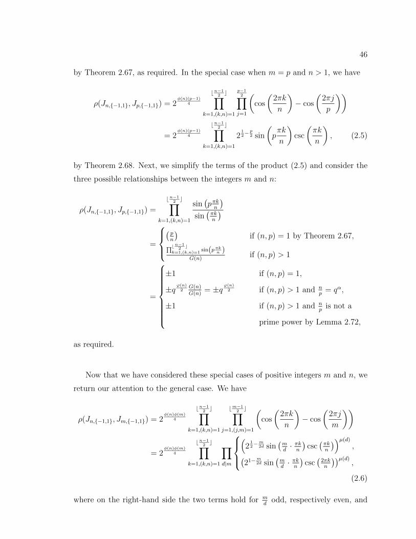
46

by Theorem 2.67, as required. In the special case when m = p and n > 1, we have

ρ(Jn,{−1,1}, Jp,{−1,1}) = 2ϕ(n)(p−1)

4

⌊n−12

⌋∏k=1,(k,n)=1

p−12∏

j=1

(cos

(2πk

n

)− cos

(2πj

p

))

= 2ϕ(n)(p−1)

4

⌊n−12

⌋∏k=1,(k,n)=1

212− p

2 sin

(pπk

n

)csc

(πk

n

), (2.5)

by Theorem 2.68. Next, we simplify the terms of the product (2.5) and consider the

three possible relationships between the integers m and n:

ρ(Jn,{−1,1}, Jp,{−1,1}) =

⌊n−12

⌋∏k=1,(k,n)=1

sin(pπk

n

)sin(πkn

)=

⎧⎪⎨⎪⎩(pn

)if (n, p) = 1 by Theorem 2.67,∏⌊n−1

2 ⌋k=1,(k,n)=1

sin(pπkn )

G(n)if (n, p) > 1

=

⎧⎪⎪⎪⎪⎪⎪⎪⎨⎪⎪⎪⎪⎪⎪⎪⎩

±1 if (n, p) = 1,

±qφ(n)2

G(n)G(n)

= ±qφ(n)2 if (n, p) > 1 and n

p= qα,

±1 if (n, p) > 1 and npis not a

prime power by Lemma 2.72,

as required.

Now that we have considered these special cases of positive integers m and n, we

return our attention to the general case. We have

ρ(Jn,{−1,1}, Jm,{−1,1}) = 2ϕ(n)ϕ(m)

4

⌊n−12

⌋∏k=1,(k,n)=1

⌊m−12

⌋∏j=1,(j,m)=1

(cos

(2πk

n

)− cos

(2πj

m

))

= 2ϕ(n)ϕ(m)

4

⌊n−12

⌋∏k=1,(k,n)=1

∏d|m

⎧⎪⎨⎪⎩(2

12−m

2d sin(md· πk

n

)csc(πkn

))µ(d),(

21−m2d sin

(md· πk

n

)csc(2πkn

))µ(d),

(2.6)

where on the right-hand side the two terms hold for mdodd, respectively even, and

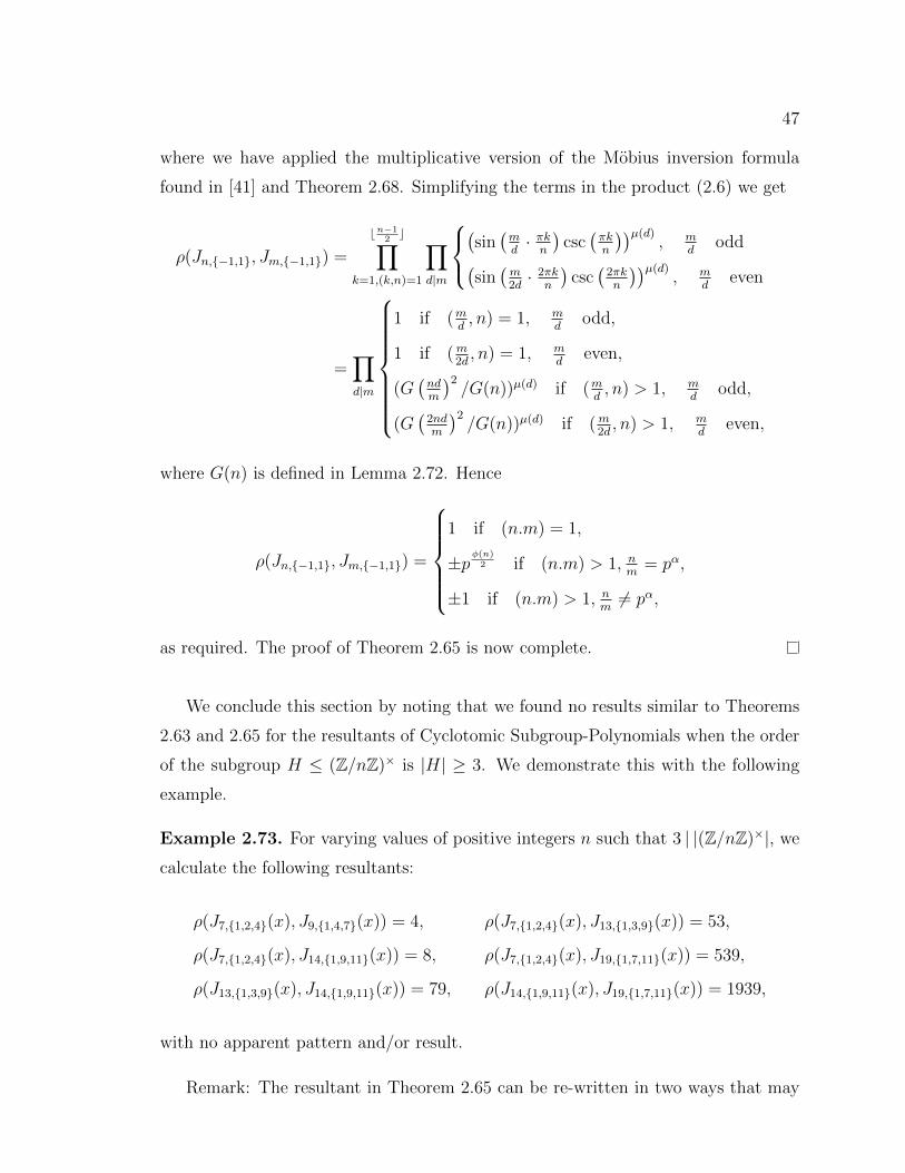
47

where we have applied the multiplicative version of the Mobius inversion formula

found in [41] and Theorem 2.68. Simplifying the terms in the product (2.6) we get

ρ(Jn,{−1,1}, Jm,{−1,1}) =

⌊n−12

⌋∏k=1,(k,n)=1

∏d|m

⎧⎨⎩(sin(md· πk

n

)csc(πkn

))µ(d), m

dodd(

sin(m2d

· 2πkn

)csc(2πkn

))µ(d), m

deven

=∏d|m

⎧⎪⎪⎪⎪⎪⎪⎪⎨⎪⎪⎪⎪⎪⎪⎪⎩

1 if (md, n) = 1, m

dodd,

1 if (m2d, n) = 1, m

deven,

(G(ndm

)2/G(n))µ(d) if (m

d, n) > 1, m

dodd,

(G(2ndm

)2/G(n))µ(d) if (m

2d, n) > 1, m

deven,

where G(n) is defined in Lemma 2.72. Hence

ρ(Jn,{−1,1}, Jm,{−1,1}) =

⎧⎪⎪⎪⎪⎨⎪⎪⎪⎪⎩1 if (n.m) = 1,

±pϕ(n)2 if (n.m) > 1, n

m= pα,

±1 if (n.m) > 1, nm

= pα,

as required. The proof of Theorem 2.65 is now complete.

We conclude this section by noting that we found no results similar to Theorems

2.63 and 2.65 for the resultants of Cyclotomic Subgroup-Polynomials when the order

of the subgroup H ≤ (Z/nZ)× is |H| ≥ 3. We demonstrate this with the following

example.

Example 2.73. For varying values of positive integers n such that 3 | |(Z/nZ)×|, wecalculate the following resultants:

ρ(J7,{1,2,4}(x), J9,{1,4,7}(x)) = 4, ρ(J7,{1,2,4}(x), J13,{1,3,9}(x)) = 53,

ρ(J7,{1,2,4}(x), J14,{1,9,11}(x)) = 8, ρ(J7,{1,2,4}(x), J19,{1,7,11}(x)) = 539,

ρ(J13,{1,3,9}(x), J14,{1,9,11}(x)) = 79, ρ(J14,{1,9,11}(x), J19,{1,7,11}(x)) = 1939,

with no apparent pattern and/or result.

Remark: The resultant in Theorem 2.65 can be re-written in two ways that may

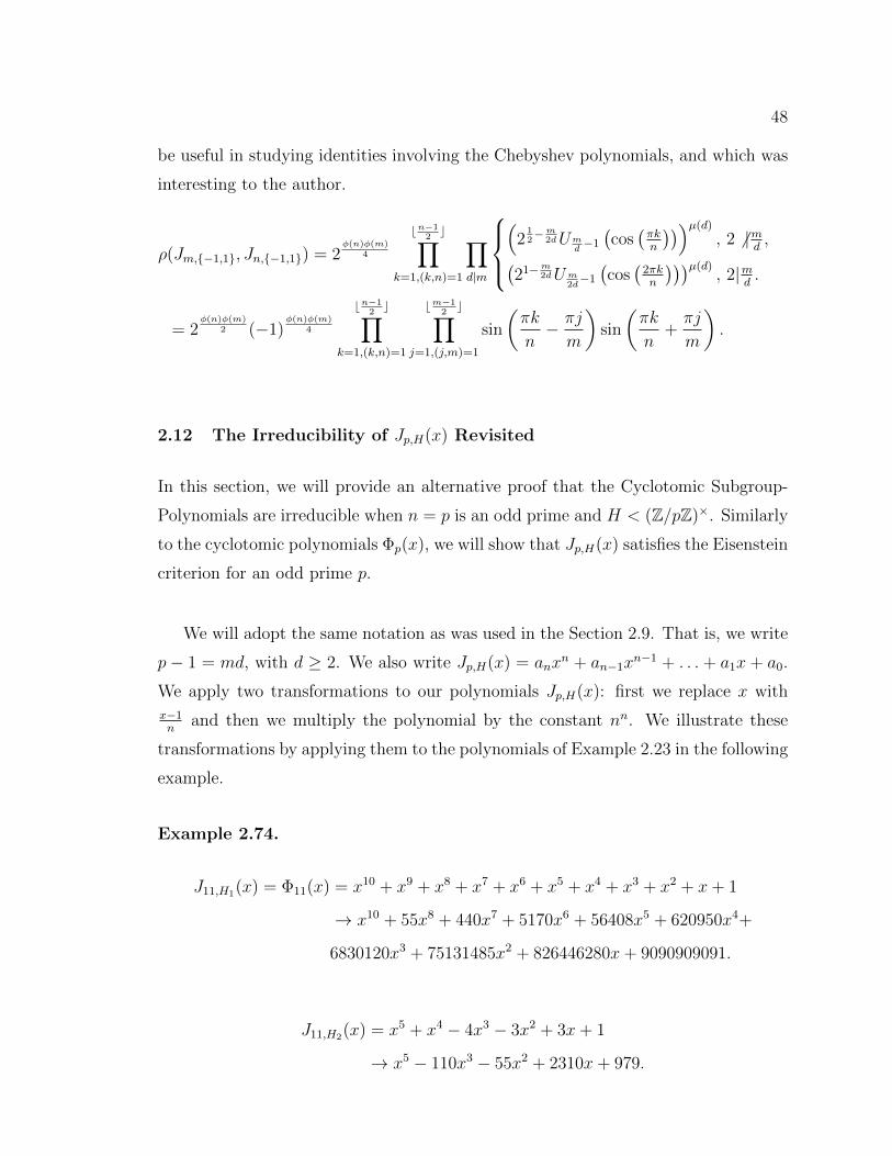
48

be useful in studying identities involving the Chebyshev polynomials, and which was

interesting to the author.

ρ(Jm,{−1,1}, Jn,{−1,1}) = 2ϕ(n)ϕ(m)

4

⌊n−12

⌋∏k=1,(k,n)=1

∏d|m

⎧⎪⎨⎪⎩(2

12−m

2dUmd−1

(cos(πkn

)))µ(d), 2 |m

d,(

21−m2dUm

2d−1

(cos(2πkn

)))µ(d), 2|m

d.

= 2ϕ(n)ϕ(m)

2 (−1)ϕ(n)ϕ(m)

4

⌊n−12

⌋∏k=1,(k,n)=1

⌊m−12

⌋∏j=1,(j,m)=1

sin

(πk

n− πj

m

)sin

(πk

n+

πj

m

).

2.12 The Irreducibility of Jp,H(x) Revisited

In this section, we will provide an alternative proof that the Cyclotomic Subgroup-

Polynomials are irreducible when n = p is an odd prime and H < (Z/pZ)×. Similarly

to the cyclotomic polynomials Φp(x), we will show that Jp,H(x) satisfies the Eisenstein

criterion for an odd prime p.

We will adopt the same notation as was used in the Section 2.9. That is, we write

p− 1 = md, with d ≥ 2. We also write Jp,H(x) = anxn + an−1x

n−1 + . . . + a1x + a0.

We apply two transformations to our polynomials Jp,H(x): first we replace x with

x−1n

and then we multiply the polynomial by the constant nn. We illustrate these

transformations by applying them to the polynomials of Example 2.23 in the following

example.

Example 2.74.

J11,H1(x) = Φ11(x) = x10 + x9 + x8 + x7 + x6 + x5 + x4 + x3 + x2 + x+ 1

→ x10 + 55x8 + 440x7 + 5170x6 + 56408x5 + 620950x4+

6830120x3 + 75131485x2 + 826446280x+ 9090909091.

J11,H2(x) = x5 + x4 − 4x3 − 3x2 + 3x+ 1

→ x5 − 110x3 − 55x2 + 2310x+ 979.

49

J11,H3(x) = x2 + x+ 3

→ x2 + 11

We note that all the modified polynomials in this example are 11-Eisenstein. This

is no coincidence:

Theorem 2.75. If p is an odd prime, then the polynomials Jp,H(x) become p-Eisenstein

polynomials for all proper subgroups H < (Z/pZ)× when x is replaced by x−1n

and the

polynomial is multiplied by the constant nn, where n = deg(Jp,H(x)) = [(Z/pZ)× : H].

Proof. We break this proof into two parts. We begin by showing that p divides all but

the leading coefficient. Then we show that p2 does not divide the constant coefficient.

Part 1. We transform Jp,H(x) by defining g(x) = nnJp,H(x−1n

). Then

g(x) = nnJp,H(x)(x−1n

)= nn

(an(x−1n

)n+ . . .+ a2

(x−1n

)2+ a1

(x−1n

)+ a0

)=

n∑j=0

nn−jaj(x− 1)j.

Now write g(x) = bnxn + . . .+ b2x

2 + b1x+ b0. Then

bi =n∑

k=i

nn−k

(k

i

)(−1)k−iak

≡d∑

k=i

dd−k−1

(k

i

)(−1)k−i

[(−1)d−k+1

(d

d− k

)md−k−1d−1

](mod p),

since d = p−1m

. Then we have:

bi ≡d∑

k=i

dd−k−1(−1)d+1−imd−k−1

(k

i

)(d

d− k

)

= dd−1md−1(−1)d+1−i

d∑k=i

(md)−k

(k

i

)(d

d− k

)

= dd−1md−1(−1)d+1−i

d∑k=i

(md)−k

(d

i

)(d− i

d− k

)(mod p),

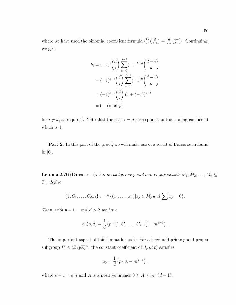
50

where we have used the binomial coefficient formula(ki

)(d

d−k

)=(di

)(d−id−k

). Continuing,

we get:

bi ≡ (−1)i(d

i

) d−i∑k=0

(−1)k+d

(d− i

k

)

= (−1)d−i

(d

i

) d−i∑k=0

(−1)k(d− i

k

)= (−1)d−i

(d

i

)(1 + (−1))d−i

= 0 (mod p),

for i = d, as required. Note that the case i = d corresponds to the leading coefficient

which is 1.

Part 2. In this part of the proof, we will make use of a result of Barcanescu found

in [6].

Lemma 2.76 (Barcanescu). For an odd prime p and non-empty subsets M1,M2, . . . ,Mn ⊆Fp, define

{1, C1, . . . , Cd−1} := #{(x1, . . . , xn)|xj ∈ Mj and∑

xj = 0}.

Then, with p− 1 = md, d > 2 we have

a0(p, d) =1

d

(p · {1, C1, . . . , Cd−1} −md−1

).

The important aspect of this lemma for us is: For a fixed odd prime p and proper

subgroup H ≤ (Z/pZ)×, the constant coefficient of Jp,H(x) satisfies

a0 =1

d

(p · A−md−1

),

where p− 1 = dm and A is a positive integer 0 ≤ A ≤ m · (d− 1).

51

Suppose, towards a contradiction, that a0 ≡ 0 (mod p2). Then

p · A−md−1 ≡ 0 (mod p2),

⇒ p · A = md−1 +Bp2,

⇒ md−1 = p · A−Bp2,

⇒ p|md−1.

This is a contradiction since p− 1 = md and p |m. This implies, in turn, that b0 ≡ 0

(mod p2) and combined with part 1 we have shown that g(x) is Eisenstein for the

odd prime p, as required.

2.13 Congruence Property

One of the properties of the cyclotomic polynomial is the fact that if n = pm, then

Φn(x) = Φp(xpm−1

). This is not true for every Cyclotomic Subgroup-Polynomial, as

we will see with the following example:

Example 2.77. We set p = 5 and take n = p2 = 25. If we choose H ≤ (Z/pZ)× to

be H = {1, 4}, then J5,H(x) = x2 + x− 1. The associated subgroup having the same

order H ′ ≤ (Z/25Z)× such that |H ′| = |H| is H ′ = {1, 24} and we have

J25,H′(x) = x10 − 10x8 + 35x6 + x5 − 50x4 − 5x3 + 25x2 + 5x− 1.

We observe that

J5,H(x5) = x10 + x5 − 1 = J25,H′(x).

However, we do note that

J25,H′(x) ≡ x10 + x5 − 1 (mod 5).

As it turns out, this is not a coincidence.

As we just saw, we do not have the direct equality that we desired; however, we

have the following analogue:

52

Theorem 2.78. If n = pm, then for each subgroup H ≤ (Z/pZ)× and associated

subgroup H ′ ≤ (Z/pmZ)× such that |H ′| = |H|, we have

Jpm,H′(x) ≡ Jp,H(xpm−1

) (mod p).

To prove Theorem 2.78, we will make use of the following theorem (this theorem

adds only a small variation to Theorem 2.3), which can be found in an Abstract

Algebra reference such as [30, pg. 35], for example.

Theorem 2.79. All subgroups of a cyclic group are cyclic. If G =< g > is a cyclic

group of order n, then for each divisor d|n there exists exactly one subgroup of order

d and it can be generated by the element gnd .

We now return to our proof.

Proof of Theorem 2.78. Let us denote w := e2πip and a := e2πi/p

m. We begin by

noting that if the element h generates the subgroup H ≤ (Z/pZ)×, then h′ = hpm−1

(mod pm) generates H ′ ≤ (Z/pmZ)×. That is,

ah′ ≡ ah

pm−1

(mod pm)

= ahp(m−1) = a(pm−1)h ≡ wh (mod p).

The roots of Jp,H and Jpm,H′ are of the form w∑

h∈H h and of the form a∑

h′∈H′ , where

the index runs through the coset representatives of H and H ′, respectively. If we then

apply the congruence ah′ ≡ wh (mod p) to each term in the summand defining the

roots, we get the required polynomial congruence.

Let us illustrate this theorem with our recurring example from this subsection:

Example 2.80. We set p = 5, n = 52 = 25, w = e2πi5 , and a = e

2πi25 . We take

H ≤ (Z/5Z)× to be H = {1, 4}. The unique subgroup of order 2 H ′ ≤ (Z/25Z)× is

53

H ′ = {1, 24}. We then calculate:

15 = 1 ≡ 1 (mod 25),

25 = 32 ≡ 7 (mod 25),

35 = 243 ≡ 18 (mod 25),

45 = 1024 ≡ 24 (mod 25);

w1 + w4 = 2 cos(2π

25), w2 + w3 = −2 cos(

π

5);

a1 + a24 = 2 cos(2π

25), a7 + a18 = −2 cos(

11π

25), . . .

Then

J5,{1,4}(x) = x2 + x− 1,

J25,{1,24}(x) = x10 − 10x8 + 35x6 + x5 − 50x4 − 5x3 + 25x2 + 5x− 1

≡ x10 + x5 − 1 (mod 5)

= J5,{1,4}(x5),

as required.

2.14 Roots

The aim of this section is to discuss the roots of the Cyclotomic Subgroup-Polynomials

for different values of n and subgroups H ≤ (Z/nZ)×. We start by considering the

roots of of the polynomials calculated in Example 2.10.

Example 2.81. As was calculated in Example 2.10, we have:

J7,H1(x) = x6 + x5 + x4 + x3 + x2 + x+ 1.

J7,H2(x) = x3 + x2 − 2x− 1.

J7,H3(x) = x2 + x+ 2.

J7,H4(x) = x− 1.

Plotting the roots of Jn,Hj(x), we have:

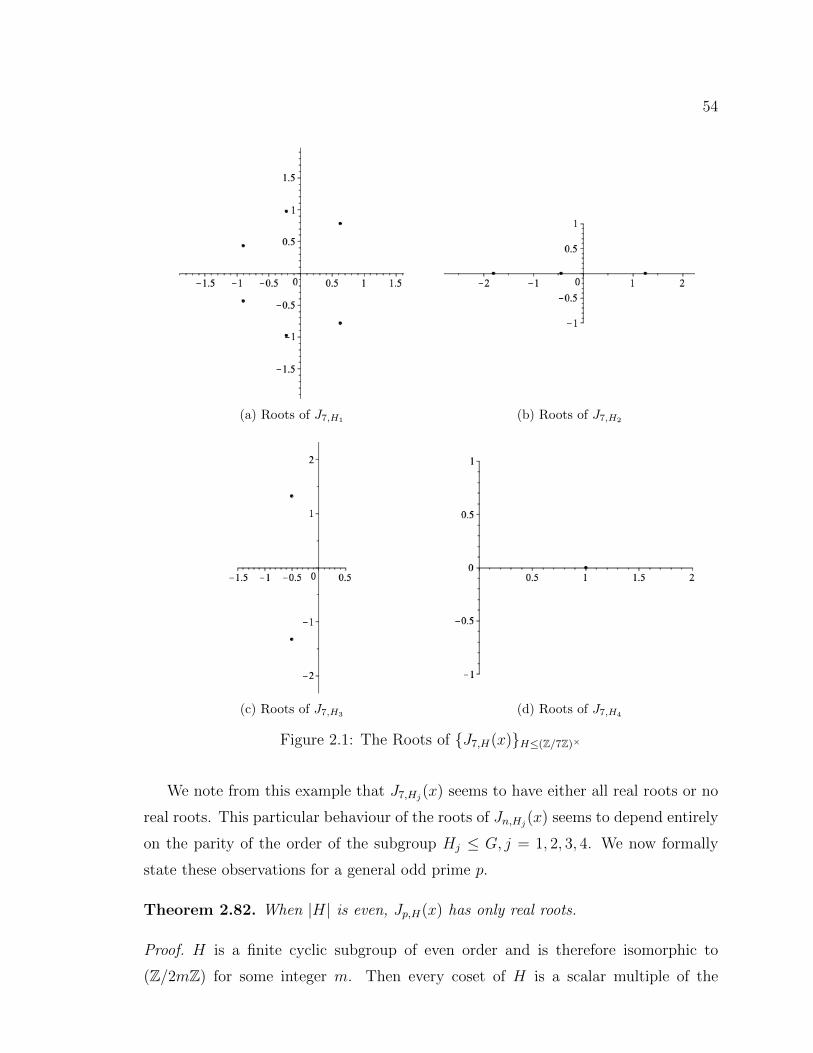
54

(a) Roots of J7,H1(b) Roots of J7,H2

(c) Roots of J7,H3 (d) Roots of J7,H4

Figure 2.1: The Roots of {J7,H(x)}H≤(Z/7Z)×

We note from this example that J7,Hj(x) seems to have either all real roots or no

real roots. This particular behaviour of the roots of Jn,Hj(x) seems to depend entirely

on the parity of the order of the subgroup Hj ≤ G, j = 1, 2, 3, 4. We now formally

state these observations for a general odd prime p.

Theorem 2.82. When |H| is even, Jp,H(x) has only real roots.

Proof. H is a finite cyclic subgroup of even order and is therefore isomorphic to

(Z/2mZ) for some integer m. Then every coset of H is a scalar multiple of the

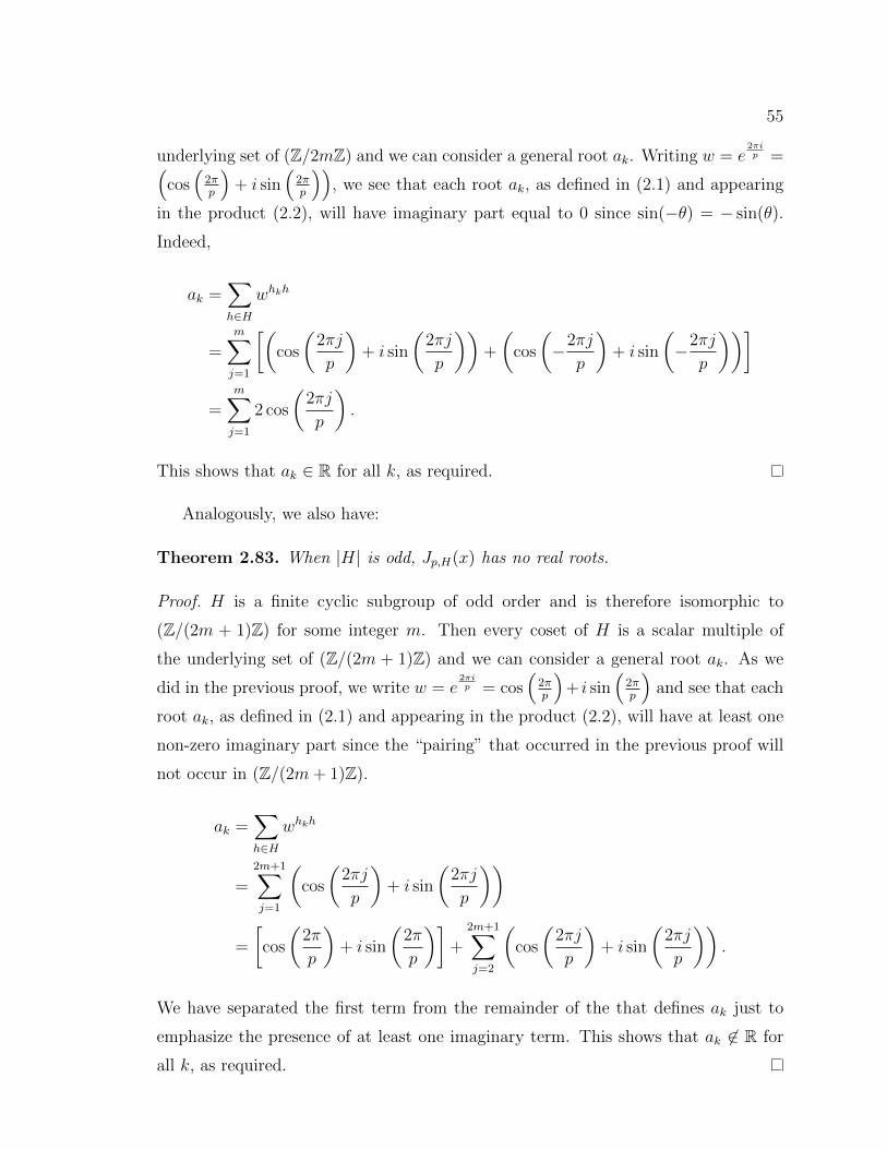
55

underlying set of (Z/2mZ) and we can consider a general root ak. Writing w = e2πip =(

cos(

2πp

)+ i sin

(2πp

)), we see that each root ak, as defined in (2.1) and appearing

in the product (2.2), will have imaginary part equal to 0 since sin(−θ) = − sin(θ).

Indeed,

ak =∑h∈H

whkh

=m∑j=1

[(cos

(2πj

p

)+ i sin

(2πj

p

))+

(cos

(−2πj

p

)+ i sin

(−2πj

p

))]

=m∑j=1

2 cos

(2πj

p

).

This shows that ak ∈ R for all k, as required.

Analogously, we also have:

Theorem 2.83. When |H| is odd, Jp,H(x) has no real roots.

Proof. H is a finite cyclic subgroup of odd order and is therefore isomorphic to

(Z/(2m + 1)Z) for some integer m. Then every coset of H is a scalar multiple of

the underlying set of (Z/(2m + 1)Z) and we can consider a general root ak. As we

did in the previous proof, we write w = e2πip = cos

(2πp

)+ i sin

(2πp

)and see that each

root ak, as defined in (2.1) and appearing in the product (2.2), will have at least one

non-zero imaginary part since the “pairing” that occurred in the previous proof will

not occur in (Z/(2m+ 1)Z).

ak =∑h∈H

whkh

=2m+1∑j=1

(cos

(2πj

p

)+ i sin

(2πj

p

))

=

[cos

(2π

p

)+ i sin

(2π

p

)]+

2m+1∑j=2

(cos

(2πj

p

)+ i sin

(2πj

p

)).

We have separated the first term from the remainder of the that defines ak just to

emphasize the presence of at least one imaginary term. This shows that ak ∈ R for

all k, as required.

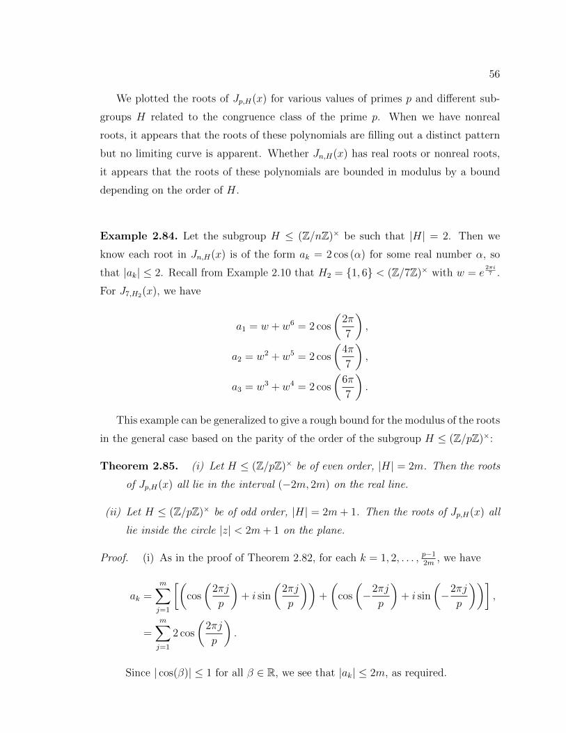
56

We plotted the roots of Jp,H(x) for various values of primes p and different sub-

groups H related to the congruence class of the prime p. When we have nonreal

roots, it appears that the roots of these polynomials are filling out a distinct pattern

but no limiting curve is apparent. Whether Jn,H(x) has real roots or nonreal roots,

it appears that the roots of these polynomials are bounded in modulus by a bound

depending on the order of H.

Example 2.84. Let the subgroup H ≤ (Z/nZ)× be such that |H| = 2. Then we

know each root in Jn,H(x) is of the form ak = 2 cos (α) for some real number α, so

that |ak| ≤ 2. Recall from Example 2.10 that H2 = {1, 6} < (Z/7Z)× with w = e2πi7 .

For J7,H2(x), we have

a1 = w + w6 = 2 cos

(2π

7

),

a2 = w2 + w5 = 2 cos

(4π

7

),

a3 = w3 + w4 = 2 cos

(6π

7

).

This example can be generalized to give a rough bound for the modulus of the roots

in the general case based on the parity of the order of the subgroup H ≤ (Z/pZ)×:

Theorem 2.85. (i) Let H ≤ (Z/pZ)× be of even order, |H| = 2m. Then the roots

of Jp,H(x) all lie in the interval (−2m, 2m) on the real line.

(ii) Let H ≤ (Z/pZ)× be of odd order, |H| = 2m+ 1. Then the roots of Jp,H(x) all

lie inside the circle |z| < 2m+ 1 on the plane.

Proof. (i) As in the proof of Theorem 2.82, for each k = 1, 2, . . . , p−12m

, we have

ak =m∑j=1

[(cos

(2πj

p

)+ i sin

(2πj

p

))+

(cos

(−2πj

p

)+ i sin

(−2πj

p

))],

=m∑j=1

2 cos

(2πj

p

).

Since | cos(β)| ≤ 1 for all β ∈ R, we see that |ak| ≤ 2m, as required.

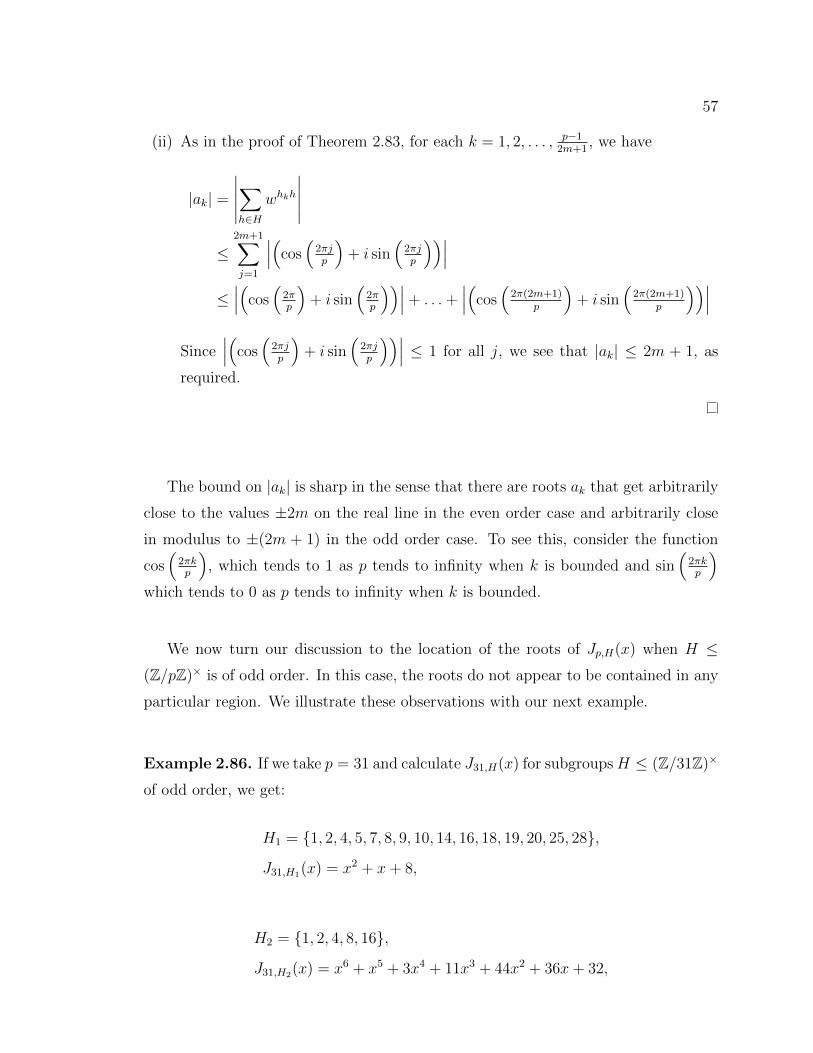
57

(ii) As in the proof of Theorem 2.83, for each k = 1, 2, . . . , p−12m+1

, we have

|ak| =∑h∈H

whkh

≤2m+1∑j=1

(cos(

2πjp

)+ i sin

(2πjp

))≤(cos(

2πp

)+ i sin

(2πp

))+ . . .+

(cos(

2π(2m+1)p

)+ i sin

(2π(2m+1)

p

))Since

(cos(

2πjp

)+ i sin

(2πjp

))≤ 1 for all j, we see that |ak| ≤ 2m + 1, as

required.

The bound on |ak| is sharp in the sense that there are roots ak that get arbitrarily

close to the values ±2m on the real line in the even order case and arbitrarily close

in modulus to ±(2m + 1) in the odd order case. To see this, consider the function

cos(

2πkp

), which tends to 1 as p tends to infinity when k is bounded and sin

(2πkp

)which tends to 0 as p tends to infinity when k is bounded.

We now turn our discussion to the location of the roots of Jp,H(x) when H ≤(Z/pZ)× is of odd order. In this case, the roots do not appear to be contained in any

particular region. We illustrate these observations with our next example.

Example 2.86. If we take p = 31 and calculate J31,H(x) for subgroupsH ≤ (Z/31Z)×

of odd order, we get:

H1 = {1, 2, 4, 5, 7, 8, 9, 10, 14, 16, 18, 19, 20, 25, 28},J31,H1(x) = x2 + x+ 8,

H2 = {1, 2, 4, 8, 16},J31,H2(x) = x6 + x5 + 3x4 + 11x3 + 44x2 + 36x+ 32,

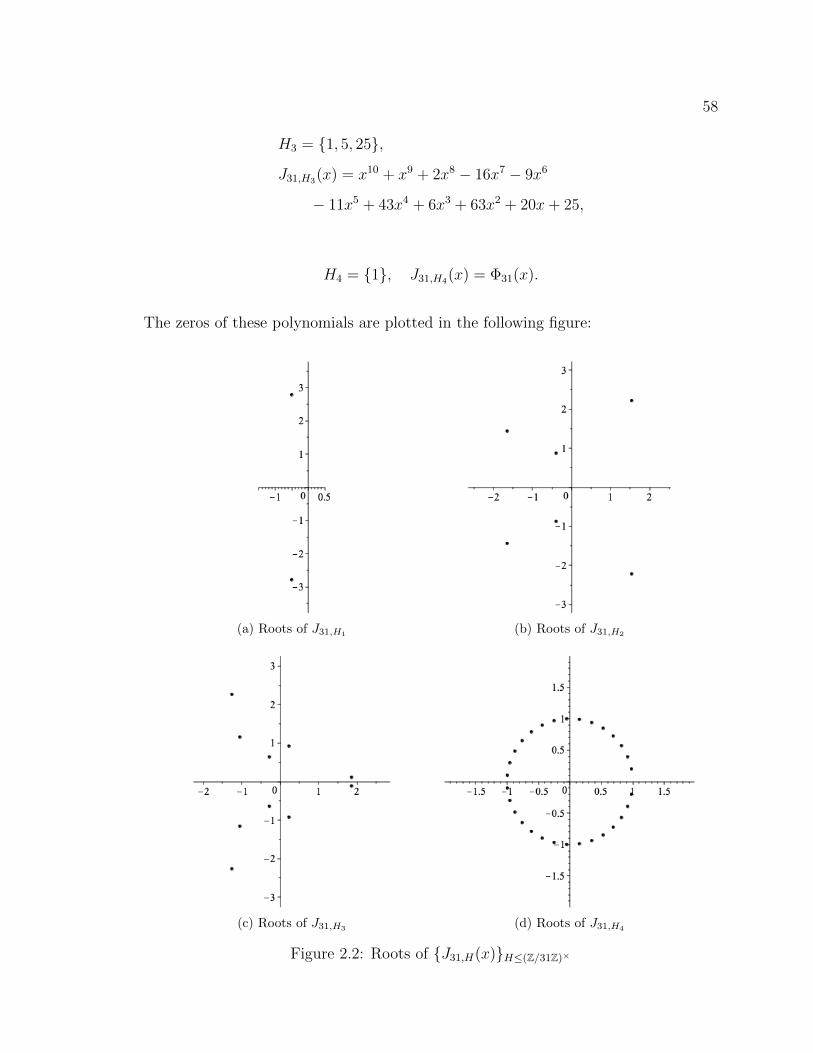
58

H3 = {1, 5, 25},J31,H3(x) = x10 + x9 + 2x8 − 16x7 − 9x6

− 11x5 + 43x4 + 6x3 + 63x2 + 20x+ 25,

H4 = {1}, J31,H4(x) = Φ31(x).

The zeros of these polynomials are plotted in the following figure:

(a) Roots of J31,H1 (b) Roots of J31,H2

(c) Roots of J31,H3(d) Roots of J31,H4

Figure 2.2: Roots of {J31,H(x)}H≤(Z/31Z)×

Chapter 3

Certain Classes of Quadrinomials

3.1 Background

For a positive integer n, the nth cyclotomic polynomial, denoted by Φn(x), is the

unique irreducible polynomial in Z[x] that divides xn − 1 but not xm − 1 for m < n.

In the special case that p is an odd prime, the cyclotomic polynomial takes the form

Φp(x) =

p−1∑k=0

xk = 1 + x+ x2 + · · ·+ xp−1, (3.1)

and the roots of this polynomial are the primitive pth roots of unity (equally spaced

around the unit circle without x = 1). One variation on the general nth cyclotomic

polynomial is obtained by keeping the leading coefficient equal to 1, but replacing the

remaining coefficients with an arbitrary positive integer c. In his investigation into

the factorization of such polynomials

fn(x) := xn + cxn−1 + cxn−2 + · · ·+ cx+ c ∈ Z[x], (3.2)

Harrington [28] posed two main questions:

(1) For what positive integers n and c is fn(x) irreducible?

(2) If fn(x) is reducible, then how does it factor?

For particular values of c, these questions have been answered. Indeed, if there

exists a prime p such that p|c but p2 |c, then the Eisenstein criterion applies and

we conclude that fn(x) is irreducible. If c = 1, the two questions become questions

related to cyclotomic polynomials and their answers are known. Harrington [28]

answers these questions in general for values of c satisfying c > 1. His main results

are as follows:

59

60

Theorem 3.1 (Harrington). Let n, c, and d be positive integers with n ≥ 3, d = c, d ≤2(c − 1), and (n, c) = (3, 3). If the trinomial h(x) = xn ± cxn−1 ± d is reducible in

Z[x], then h(x) = (x± 1)g(x) for some irreducible g(x) ∈ Z[x].

This theorem is then used to answer the two initial questions with the following

theorem below.

Theorem 3.2 (Harrington). Let n and c be positive integers with c ≥ 2. Then the

polynomials

f(x) = xn +n−1∑j=0

cxj, g(x) = xn +n−1∑j=0

(−1)n−jcxj,

h(x) = xn −n−1∑j=0

cxj, k(x) = xn −n−1∑j=0

(−1)n−jcxj,

are irreducible in Z[x] with the exceptions of f(x) = x2 + 4x + 4 = (x + 2)2 and

g(x) = x2 − 4x+ 4 = (x− 2)2.

It is the purpose of this chapter to obtain analogous results for the modified case

concerning polynomials of the form

xn + cxn−a−1 + cxn−a−2 + · · ·+ cx+ c ∈ Z[x], (3.3)

where a and c are positive integers. In other words, we will investigate analogues to

(3.2) with a gap after the leading coefficients. To align our notation with the original

notation found in [28], we make the following definition.

Definition 3.3. Let n, c and a be positive integers with c ≥ 2 and a < n. Then

denote:

fa,cn (x) = xn +

n−a−1∑j=0

cxj, ga,cn (x) = xn +n−a−1∑j=0

(−1)n−jcxj,

ha,cn (x) = xn −

n−a−1∑j=0

cxj, ka,cn (x) = xn −

n−a−1∑j=0

(−1)n−jcxj.

61

3.2 Irreducibility

In pursuit of an analogue to Theorem 3.1, we can multiply (3.3) by a linear factor

(x± 1). However, in this case, instead of the resulting polynomial being a trinomial

we actually get a quadrinomial. More specifically, our resulting quadrinomials are of

the form:

(x− 1)fa,cn (x) = xn+1 − xn + cxn−a − c,

(x+ 1)ga,cn (x) =

⎧⎨⎩xn+1 + xn − cxn−a + c if n− a ≡ 0 (mod 2),

xn+1 + xn + cxn−a + c if n− a ≡ 1 (mod 2),

(x− 1)ha,cn (x) = xn+1 − xn − cxn−a + c,

(x+ 1)ka,cn (x) =

⎧⎨⎩xn+1 + xn + cxn−a − c if n− a ≡ 0 (mod 2),

xn+1 + xn − cxn−a − c if n− a ≡ 1 (mod 2).

Unlike the case with Theorem 3.1, we are unable to determine the factorizations

of these quadrinomials in the most general case. We will make an additional comment

regarding an analogue to Theorem 3.1 in the conclusion of the thesis.

Similar to the case with Theorem 3.2, there are special factorizations of fa,cn , ga,cn , ha,c

n ,

and ka,cn that are known. For example, when c = sn is a perfect nth power, we have:

xn − c = (x− s)(xn−1 + sxn−2 + s2xn−3 + . . .+ sn−1), (3.4)

xn + c = (x+ s)(xn−1 − sxn−2 + s2xn−3 − . . .+ sn−1) if n is odd. (3.5)

Already this contrasts with Theorem 3.1 in the sense that we have infinitely many

exceptional cases. These are not the only reducible cases of fa,cn , ga,cn , ha,c

n , and ka,cn as

we will see in the following example.

Example 3.4. We have the following factorizations of f 3,86 (x) and h6,81

8 (x) respec-

tively:

f 3,86 (x) = x6 + 8x2 + 8x+ 8 = (x2 + 2x+ 2)(x4 − 2x3 + 2x2 + 4),

h6,818 (x) = x8 − 81x− 81 = (x2 + 3x+ 3)(x6 − 3x5 + 6x4 − 9x3 + 9x2 − 27).

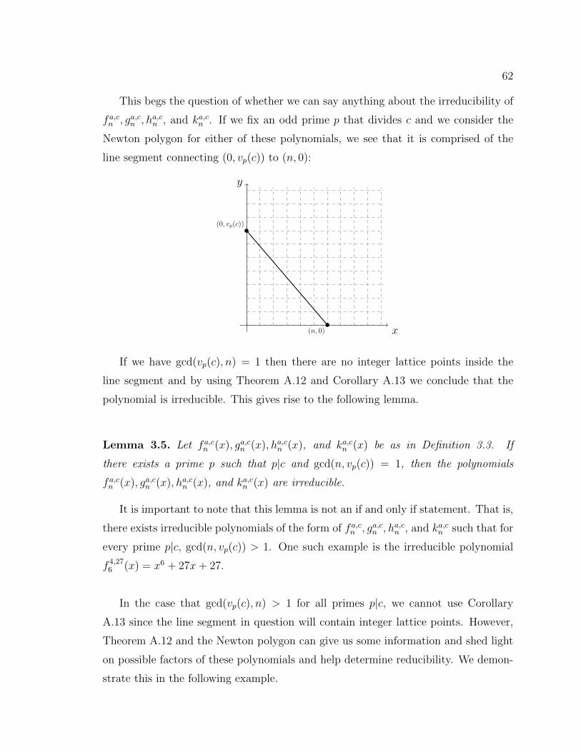
62

This begs the question of whether we can say anything about the irreducibility of

fa,cn , ga,cn , ha,c

n , and ka,cn . If we fix an odd prime p that divides c and we consider the

Newton polygon for either of these polynomials, we see that it is comprised of the

line segment connecting (0, vp(c)) to (n, 0):

(0, vp(c))

(n, 0) x

y

If we have gcd(vp(c), n) = 1 then there are no integer lattice points inside the

line segment and by using Theorem A.12 and Corollary A.13 we conclude that the

polynomial is irreducible. This gives rise to the following lemma.

Lemma 3.5. Let fa,cn (x), ga,cn (x), ha,c

n (x), and ka,cn (x) be as in Definition 3.3. If

there exists a prime p such that p|c and gcd(n, vp(c)) = 1, then the polynomials

fa,cn (x), ga,cn (x), ha,c

n (x), and ka,cn (x) are irreducible.

It is important to note that this lemma is not an if and only if statement. That is,

there exists irreducible polynomials of the form of fa,cn , ga,cn , ha,c

n , and ka,cn such that for

every prime p|c, gcd(n, vp(c)) > 1. One such example is the irreducible polynomial

f 4,276 (x) = x6 + 27x+ 27.

In the case that gcd(vp(c), n) > 1 for all primes p|c, we cannot use Corollary

A.13 since the line segment in question will contain integer lattice points. However,

Theorem A.12 and the Newton polygon can give us some information and shed light

on possible factors of these polynomials and help determine reducibility. We demon-

strate this in the following example.

63

Example 3.6. Let p be a prime and consider the polynomial f 4,p4

6 (x) = x6+p4x+p4.

We then have gcd(n, vp(c)) = gcd(6, 4) = 2 and the Newton polygon is the line

segment joining the points (0, 4) and (6, 0) which contains the integer lattice point

(3, 2). This tells us that if this polynomial factors, it factors as two cubic polynomials

where p2 divides the constant coefficient and the coefficient of x and p divides the

coefficient of x2 in each one. That is,

f 4,p4

6 (x) =(x3 + Apx2 +Bp2x+ Cp2

) (x3 + A′px2 +B′p2x+ C ′p2

). (3.6)

Comparing the constant coefficient on both sides of (3.6), we see that C = C ′ = 1.

We then have

f 4,p4

6 (x) =(x3 + Apx2 +Bp2x+ p2

) (x3 + A′px2 +B′p2x+ p2

). (3.7)

Comparing the coefficient of x5 on both sides of (3.7), we see that A′p + Ap = 0 or

A′ = −A. We then have

f 4,p4

6 (x) =(x3 + Apx2 +Bp2x+ p2

) (x3 − Apx2 +B′p2x+ p2

). (3.8)

Comparing the coefficient of x4 on both sides of (3.8), we see that B′p2+Bp2−A2p2 =

0 or B′ +B − A2 = 0. Comparing the coefficient of x3 on both sides of (3.8), we see

that 2p2 + AB′p3 − ABp3 = 0 or −Ap(B′ − B) = 2. This last equation indicates to

us that if our system of equations has a solution (i.e., f 4,p4

6 (x) is possibly reducible),

the only option is p must be equal to 2. We substitute p = 2 and see that indeed:

f 4,166 (x) = x6 + 16x+ 16 = (x3 − 2x2 + 4)(x3 + 2x2 + 4x+ 4).

This example allows us to state the following lemma:

Lemma 3.7. Let p be a prime and f 4,p4

6 (x) = x6+ p4x+ p4. Then f 4,p4

6 is irreducible

for all odd primes p and reducible for the prime p = 2.

To illustrate that this type of argument will not work in the most general case,

consider the polynomial f 12,37

14 (x) = x14+2187x+2187 which is reducible and factors

as a product of an irreducible quadratic and an irreducible polynomial of degree 12.

64

We will now consider another example illustrating the use of Newton polygons to

help determine the irreducibility of f 4,q3·p46 (x).

Example 3.8. Let p and q be distinct primes and consider the polynomial f 4,q3·p46 (x) =

x6 + q3p4x + q3p4. If we consider the Newton Polygon for this polynomial with re-

spect to q we see that it is comprised of the line segment joining the points (0, 3) and

(6, 0). This line segment contains the integer lattice points (2, 2) and (4, 1) which in-

dicates that if this polynomial does factor, it will do so as a product of an irreducible

quadratic and an irreducible quartic or as the product of three irreducible quadratics.

If we consider the Newton Polygon for this polynomial with respect to p we see that

is comprised of the line segment joining the points (0, 4) and (6, 0). This line segment

contains the integer lattice point (3, 2) which indicates that if this polynomial does

factor, it will do so as a product of two irreducible cubics. Since there is no way

to reconcile these possible factorizations, we conclude that this polynomial must be

irreducible.

The argument presented in this example was actually independent of the param-

eter a and allows us to state the following lemma.

Lemma 3.9. For distinct primes p and q and integer 0 ≤ a ≤ 5 the polynomial

fa,q3·p46 (x) = x6 + q3p4xn−a−1 + . . .+ q3p4x+ q3p4 is irreducible.

We now generalize the previous example for a special form of the integer c.

Example 3.10. Consider the polynomial fa,c30 (x) where c = p61 · p102 · p153 for distinct

primes p1, p2, and p3. We have n = 30 = 2 · 3 · 5 and gcd(6, 10, 15) = gcd(2, 15) = 1.

If we consider the Newton polygon of p1, p2, and p3 respectively we see that if fa,c30

was to be reducible:

(i) fa,c30 must factor as a product of at most 6 irreducible factors and the degree of

each factor needs to be a multiple of 5,

(ii) fa,c30 must factor as a product of at most 10 irreducible factors and the degree of

each factor needs to be a multiple of 3,

(iii) fa,c30 must factor as a product of at most 15 irreducible factors and the degree of

each factor needs to be a multiple of 2.

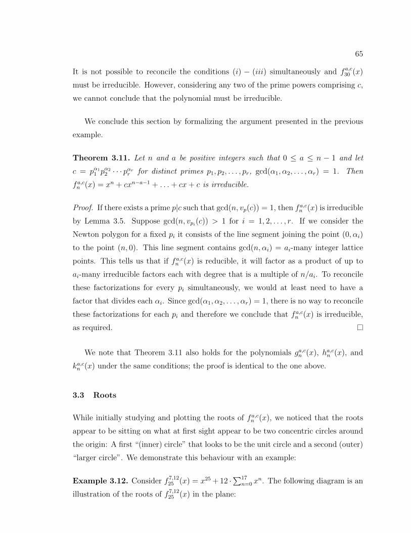
65

It is not possible to reconcile the conditions (i) − (iii) simultaneously and fa,c30 (x)

must be irreducible. However, considering any two of the prime powers comprising c,

we cannot conclude that the polynomial must be irreducible.

We conclude this section by formalizing the argument presented in the previous

example.

Theorem 3.11. Let n and a be positive integers such that 0 ≤ a ≤ n − 1 and let

c = pα11 pα2

2 · · · pαrr for distinct primes p1, p2, . . . , pr, gcd(α1, α2, . . . , αr) = 1. Then

fa,cn (x) = xn + cxn−a−1 + . . .+ cx+ c is irreducible.

Proof. If there exists a prime p|c such that gcd(n, vp(c)) = 1, then fa,cn (x) is irreducible

by Lemma 3.5. Suppose gcd(n, vpi(c)) > 1 for i = 1, 2, . . . , r. If we consider the

Newton polygon for a fixed pi it consists of the line segment joining the point (0, αi)

to the point (n, 0). This line segment contains gcd(n, αi) = ai-many integer lattice

points. This tells us that if fa,cn (x) is reducible, it will factor as a product of up to

ai-many irreducible factors each with degree that is a multiple of n/ai. To reconcile

these factorizations for every pi simultaneously, we would at least need to have a

factor that divides each αi. Since gcd(α1, α2, . . . , αr) = 1, there is no way to reconcile

these factorizations for each pi and therefore we conclude that fa,cn (x) is irreducible,

as required.

We note that Theorem 3.11 also holds for the polynomials ga,cn (x), ha,cn (x), and

ka,cn (x) under the same conditions; the proof is identical to the one above.

3.3 Roots

While initially studying and plotting the roots of fa,cn (x), we noticed that the roots

appear to be sitting on what at first sight appear to be two concentric circles around

the origin: A first “(inner) circle” that looks to be the unit circle and a second (outer)

“larger circle”. We demonstrate this behaviour with an example:

Example 3.12. Consider f 7,1225 (x) = x25 +12 ·∑17

n=0 xn. The following diagram is an

illustration of the roots of f 7,1225 (x) in the plane:

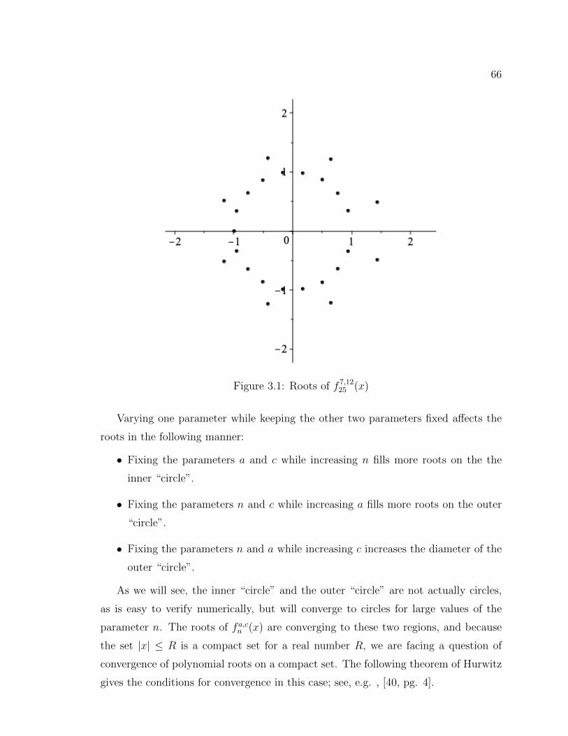
66

Figure 3.1: Roots of f 7,1225 (x)

Varying one parameter while keeping the other two parameters fixed affects the

roots in the following manner:

• Fixing the parameters a and c while increasing n fills more roots on the the

inner “circle”.

• Fixing the parameters n and c while increasing a fills more roots on the outer

“circle”.

• Fixing the parameters n and a while increasing c increases the diameter of the

outer “circle”.

As we will see, the inner “circle” and the outer “circle” are not actually circles,

as is easy to verify numerically, but will converge to circles for large values of the

parameter n. The roots of fa,cn (x) are converging to these two regions, and because

the set |x| ≤ R is a compact set for a real number R, we are facing a question of

convergence of polynomial roots on a compact set. The following theorem of Hurwitz

gives the conditions for convergence in this case; see, e.g. , [40, pg. 4].

67

Theorem 3.13 (Hurwitz). Let fn(z) (n = 1, 2, . . .) be a sequence of functions which

are analytic in a region D and which converge uniformly to a function f(z) ≡ 0 in

every closed subregion of D. Let ζ be an interior point of D. If ζ is a limit point of

the zeros of the fn(z), then ζ is a zero of f(z). Conversely, if ζ is an m-fold zero of

f(z), every sufficiently small neighbourhood K of ζ contains exactly m zeros (counted

with their multiplicities) of each fn(z), n ≥ N(K).

Thus, if we can find a function Q(x) such that the roots of fa,cn (x) are converging

to the roots of Q(x) uniformly on a compact subset, we can exactly describe the

limiting curve of the roots of fa,cn (x). Through computational experimentation we

find the visual comparison below.

(a) Roots of (x15 − x14 + 25)(∑35

j=0 xj) (b) Roots of f15,25

50 (x)

Figure 3.2: Comparison of Roots of Degree 50

If the parameter n (degree) is increased, that is, if we add more roots to the

polynomials fa,cn (x) and compare them to one another, we observe that the comparison

strengthens.

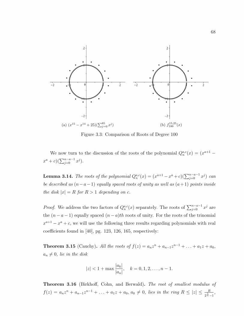
68

(a) (x15 − x14 + 25)(∑85

j=0 xj) (b) f15,25

100 (x)

Figure 3.3: Comparison of Roots of Degree 100

We now turn to the discussion of the roots of the polynomial Qa,cn (x) = (xa+1 −

xa + c)(∑n−a−1

j=0 xj).

Lemma 3.14. The roots of the polynomial Qa,cn (x) = (xa+1−xa+ c)(

∑n−a−1j=0 xj) can

be described as (n−a−1) equally spaced roots of unity as well as (a+1) points inside

the disk |x| = R for R > 1 depending on c.

Proof. We address the two factors of Qa,cn (x) separately. The roots of

∑n−a−1j=0 xj are

the (n− a− 1) equally spaced (n− a)th roots of unity. For the roots of the trinomial

xa+1 − xa + c, we will use the following three results regarding polynomials with real

coefficients found in [40], pg. 123, 126, 165, respectively:

Theorem 3.15 (Cauchy). All the roots of f(z) = anzn + an−1z

n−1 + . . .+ a1z + a0,

an = 0, lie in the disk

|z| < 1 + max|ak||an|

, k = 0, 1, 2, . . . , n− 1.

Theorem 3.16 (Birkhoff, Cohn, and Berwald). The root of smallest modulus of

f(z) = anzn + an−1z

n−1 + . . . + a1z + a0, a0 = 0, lies in the ring R ≤ |z| ≤ R

21n−1

,

69

where R is the positive root of of the equation

|a0| − |a1|z − |a2|z2 − . . .− |an|zn = 0.

Theorem 3.17 (Nekrasoff, Kempner, Herglotz, and Biernacki). The trinomial αzn+

zp +1 for α ∈ R, n, p ∈ N with 0 < p < n, has at least one root in each of the sectorsArg (z)− (2k + 1)p

π

≤ π

n, k = 0, 1, . . . , p− 1.

We apply Theorem 3.15 to conclude that the roots of xa+1 − xa + c lie inside the

circle |x| < 1 + |c|. We then apply Theorem 3.16 to conclude that all of the roots of

xa+1 − xa + c satisfy |x| > 1. Lastly, to apply Theorem 3.17, we note the following

transformation:

q(z) = bza+1 + za + 1,

q(−z

b

)= b

(−z

b

)a+1

+(−z

b

)a+ 1,

= (−1)a+1 1

ba(za+1 − za) + 1.

This implies that

−(−b)aq(−z

b

)= za+1 − za − (−b)a.

If we set c = | − (−b)a| (replacing b with −b if necessary) we can now apply Theorem

3.17 to the trinomial xa+1 − xa + c.

Putting it all together, we have shown that the roots of Qa,cn are made up of

(n − a − 1) roots of unity and an additional (a + 1) roots that lie in the disk 1 <

|x| < 1+ c and have angular distribution as described in Theorem 3.17. We have now

demonstrated all of the required properties and have proven Lemma 3.14.

We are now in a position to apply Theorem 3.13 to fa,cn (x).

Theorem 3.18. For fixed natural numbers a, n, c with 0 < a < n, the roots of the

70

polynomial fa,cn (x) = xn + cxn−a−1 + cxn−a−2 + cxn−a−3 + · · ·+ cx+ c converge to the

roots of the polynomial (xa+1 − xa + c) and to the unit circle as n → ∞.

Proof. We begin by noting the identity

fa,cn (x) = xn + cxn−a−1 + cxn−a−2 + · · ·+ cx+ c

= (xa+1 − xa + c)

(n−a−1∑j=0

xj

)+ xa. (3.9)

We set N = n− a− 1 and note that as n → ∞, N → ∞. We re-write (3.9) as

fa,cn (x) = (xa+1 − xa + c)

(N∑j=0

xj

)+ xa (3.10)

and we consider the following two cases based on |x|. Let ϵ > 0 be arbitrary.

(i) Case 1: |x| ≤ 1− ϵ. As N → ∞, the geometric series∑N

j=0 xj, converges to 1

1−x

and the difference between the two sides of (3.10) is equal to xn which converges

uniformly to zero as n → ∞ for |x| ≤ 1− ϵ.

(ii) Case 2: |x| ≥ 1 + ϵ. We replace x with 1xand proceed as in the previous case.

This time, as N → ∞, the difference between the two sides of (3.10) is equal to(1x

)nwhich converges uniformly to zero as n → ∞ for |x| ≥ 1 + ϵ.

Since ϵ is arbitrary and can be made as small as we like, we see that as n → ∞,

fa,cn (x) converges to the function (xa+1 − xa + c)(

∑Nj=0 x

j) where N is an arbitrarily

large positive integer. Then the conditions of Theorem 3.13 are met and we can apply

this theorem to conclude our desired result, Theorem 3.18.

Although we used fa,cn (x) explicitly in the statement and proof of Theorem 3.18,

the result also applies to ga,cn (x), ka,cn (x), and ha,c

n (x). To see this, note the following

relationships between our polynomials:

ha,cn (x) = (xa+1 − xa − c)

(n−a−1∑j=0

xj

)+ xa,

ga,cn (x) = fa,cn (x),

ka,cn (x) = ha,c

n (−x).

71

3.4 Discriminants

In this section we will introduce the very basics of the concept of the discriminant of

a polynomial, just enough for our use. For a detailed and thorough treatment of the

topic, the reader is referred to [49, ppg. 23–28].

Let f and g be two polynomials with real coefficients, given by

f(x) = anxn + an−1x

n−1 + · · ·+ a1x+ a0, an = 0,

g(x) = bmxm + bm−1x

m−1 + · · ·+ b1x+ b0 bm = 0.

The resultant of f(x) and g(x) is defined by the determinant of a certain (m+ n)×(m+ n) matrix which has the coefficients of f(x) and g(x) or 0 as entries; we denote

it by ρ(f, g). The resultant was discussed in further detail earlier in this thesis in

Subsection 2.11. The discriminant of a polynomial f(x) is then defined as

D(f) =(−1)

n(n+1)2

anρ(f, f ′),

where f ′ denotes the derivative of f(x).

The discriminant of a polynomial is a polynomial function of the coefficients ai,

which provides some insight into the roots of the polynomials without requiring their

computation. The canonical example is the quadratic polynomial ax2+ bx+ c ∈ R[x]which has discriminant b2 − 4ac. If b2 − 4ac < 0 then the quadratic has no real roots,

if b2− 4ac > 0 then the quadratic has two distinct real roots, and if b2− 4ac = 0 then

the quadratic has a single real root with multiplicity two. In general, a polynomial

with real coefficients has a multiple root if and only if the discriminant is zero. If the

roots of the polynomial are known, the discriminant can be calculated in terms of the

roots as well.

Lemma 3.19. The discriminants of fa,cn (x), ga,cn (x), ha,c

n (x), and ka,cn (x) are congruent

to zero modulo c for n ≥ 2.

72

Proof. Since the discriminant is a polynomial function in the coefficients of our poly-

nomials and reduction modulo c is a ring homomorphism on Z, we have

D(fa,cn (x)) ≡ D(ga,cn (x)) ≡ D(ha,c

n (x)) ≡ D(ka,cn (x)) (mod c),

≡ D(xn) (mod c),

= 0 for n ≥ 2,

as required.

When calculating the discriminants of fa,cn (x), ga,cn (x), ha,c

n (x), and ka,cn (x), we no-

tice that not only are they congruent to 0 modulo c, but that a higher power of c

divides the discriminant. We demonstrate this with an example using fa,cn (x).

Example 3.20.

D(f 1,c3 (x)) = −3c4 + 14c3 − 27c2,

D(f 1,c4 (x)) = −12c5 − 11c4 + 256c3,

D(f 1,c5 (x)) = 64c7 − 48c6 − 84c5 + 3125c4,

D(f 2,c3 (x)) = −27c2,

D(f 2,c4 (x)) = −27c4 + 256c3,

D(f 2,c5 (x)) = 81c6 + 906c5 + 3125c4.

This leads us to the following stronger result:

Theorem 3.21. For fa,cn (x), ga,cn (x), ha,c

n (x), and ka,cn (x), we have

D(fa,cn (x)) ≡ D(ga,cn (x)) ≡ D(ha,c

n (x)) ≡ D(ka,cn (x)) ≡ 0 (mod cn−1),

for all n ≥ 2 and all values of a and c.

Proof. To prove Theorem 3.21, we will make use of the following result regarding

discriminants of polynomials, which can be found in [32], for example.

Theorem 3.22 (Theorem 1.4 [32]). (i) The discriminant of a polynomial f is ho-

mogenous of degree (2n− 2) in the coefficients a0, a1, . . . , an.

73

(ii) If ai is regarded as having degree i in the discriminant, then the discriminant of

f is homogenous of degree n(n− 1).

Since the coefficients of fa,cn (x), ga,cn (x), ha,c

n (x), and ka,cn (x) all share the structure:

an = 1 and ai = c for i = 0, 1, 2, . . . , (n − a − 1), parts (i) and (ii) combine to

allow us to conclude that the discriminants of fa,cn (x), ga,cn (x), ha,c

n (x), and ka,cn (x) are

homogenous in the term 1n · cn−1 = cn−1 as required.

Remark: The author was made aware of a more direct approach to proving The-

orem 3.21. One of the examiners notes that Theorem 3.21 follows directly by looking

at the Sylvester matrix associated with the polynomials; they will have n− 1 columns

on the right where each element of the column is divisible by c and so the determinant

is divisible by cn−1.

3.5 Results About Related Trinomials and Quadrinomials

Although not applicable to the trinomials studied by Harrington in [28] or the quadri-

nomials mentioned in this chapter, we came across similar and interesting results in

the literature for certain special cases of these polynomials.

The authors of [19] study the following three types of polynomials:

Definition 3.23. A polynomial xn + an−1xn−1 + . . . + a1x + a0 with ak ∈ {0, 1} for

all 1 ≤ k ≤ n− 1 and a0 = 1 is called a Newman polynomial.

Definition 3.24. A polynomial anxn + an−1x

n−1 + . . . + a1x + a0 with ak ∈ {−1, 1}for all k is called a Littlewood polynomial.

Definition 3.25. A polynomial anxn+an−1x

n−1+ . . .+a1x+a0 with ak ∈ {−1, 0, 1}for all k and a0 = 0 is called a Borwein polynomial.

In [22], the author considers many interesting results on the geometry of the roots

of trinomials. For results on the irreducibility of trinomials and quadrinomials with

coefficients restricted to some subset of the set {−p,−1, 0, 1, p} where p is an odd

prime, the reader is referred to [23], [39], [45], and [46].

74

The books [5], [11], [40], and [49] contain many useful and interesting results on

the reducibility and roots of polynomials in general.

Chapter 4

Binomial Congruences and Honda’s Congruences

4.1 Background

Wilson’s theorem and its converse due to Lagrange combine to give a criterion for

identifying the prime numbers:

Theorem 4.1 (Wilson and Lagrange). A positive integer p > 1 is a prime if and

only if (p− 1)! ≡ −1 (mod p).

A famous binomial coefficient congruence, due to J. Wolstenholme, states

Theorem 4.2 (Wolstenholme). For any prime, p ≥ 5,(2p− 1

p− 1

)≡ 1 (mod p3).

Unlike Wilson’s theorem, a converse to Wolstenholme’s theorem has not been es-

tablished. But Theorem 4.2 has no composite solutions, n < 109, such that(2n−1n−1

)≡ 1

(mod n3). It has been conjectured that no composite solutions exist and that Wol-

stenholme’s theorem, like Wilson’s theorem, also gives a criterion for identifying the

prime numbers. For a more detailed and complete presentation of Theorem 4.2, the

reader is referred to [31] or [43].

Theorem 4.2 may be rewritten as

Theorem 4.3. For any prime, p ≥ 5,(2p

p

)≡ 2 (mod p3).

Wolstenholme’s theorem was generalized by W. Ljunggren [26] to

75

76

Theorem 4.4 (Ljunggren). For any prime, p ≥ 5, and nonnegative integers n,m we

have (np

mp

)≡(n

m

)(mod p3).

In two of their joint papers [13] and [14], M. Chamberland and K. Dilcher studied

a class of binomial sums,

uϵa,b(n) :=

n∑k=0

(−1)ϵk(n

k

)a(2n

k

)b

, (4.1)

and their divisibility properties. In particular, when a = b = ϵ = 1, they proved the

following analogue of Ljunggren’s theorem.

Theorem 4.5 ([14], Theorem 2.1). For all primes p ≥ 5 and integers m ≥ 1 we have

u(mp) ≡ u(m) (mod p3),

where u(n) := u11,1(n).

4.2 Parameter Introduced

In a paper by D.F. Bailey [4] the following parameterized version of Ljunggren’s

theorem is presented.

Theorem 4.6 (Bailey). For any prime p ≥ 5 and nonnegative integers m,n, s we

have (mps+1

nps+1

)≡(mps

nps

)(mod ps+3).

Of particular interest to us is an identity that appears on page 124 of [4] during

the proof of Theorem 4.6:

Lemma 4.7 (Bailey). For any prime p ≥ 5 and nonnegative integers m,n, s we have(mps+1

lp

)≡(mps

l

)(mod ps+3). (4.2)

77

Following in the footsteps of Chamberland and Dilcher [14], we present the fol-

lowing new result.

Theorem 4.8. For any prime p ≥ 5 and nonnegative integers m, s we have

u(mps+1) ≡ u(mps) (mod ps+3).

To prove this result we first note that the case s = 0 is the case proved in [14]; we

will therefore assume that s ≥ 1. We express the sum (4.1) for a = b = ϵ = 1 as

u(mps+1) :=

mps+1∑k=0

(−1)k(mps+1

k

)(2mps+1

k

)

=

mps−1∑k=0

p−1∑j=1

(−1)pk+j

(mps+1

pk + j

)(2mps+1

pk + j

)

+

mps∑k=0

(−1)pk(mps+1

pk

)(2mps+1

pk

). (4.3)

The proof is made up of two parts: first we show that the double sum is congruent

to 0 modulo ps+3, and then we use the fact that p is odd and apply Lemma 4.7 term

by term to second sum of (4.3).

Lemma 4.9. Let m, s, and j be positive integers with 1 ≤ j ≤ p− 1. Then the power

of the odd prime p dividing(mps+1

pk+j

)and

(2mps+1

pk+j

)is at least vp(mps+1).

Proof. We will consider the first binomial coefficient and note that the case of the

second follows in an analogous manner, since vp(mps+1) = vp(2mps+1). We have(mps+1

pk + j

)=

(mps+1)!

(pk + j)!(mps+1 − pk − j)!

=(mps+1) · · · (mps+1 − pk − j + 1)

(pk + j) · · · (2)(1) . (4.4)

To ensure that the p-adic valuation of the binomial coefficient is indeed at least the p-

adic valuation of mps+1, we need to show that the p-adic valuation of the denominator

of (4.4) is less than or equal to the p-adic valuation of (mps+1 − 1)!. After some

simplification, we need to show that, for fixed p, k, and j as in the statement of

78

Lemma 4.9, we have:

vp

(pk+j∏i=1

i

)≤ vp

⎛⎝ mps+1−1∏i=mps+1−pk−j+1

i

⎞⎠ . (4.5)

The product on the left-hand side of the inequality (4.5) contains (pk+j) consecutive

terms with an initial term equal to 1 while the product on the right-hand side of the

inequality (4.5) contains (pk + j − 1) consecutive terms with an initial term greater

than 1. Since p is an odd prime, we know that the first two terms of the product on the

left-hand side satisfy vp(i) = 0, and therefore our inequality holds, as required.

Proof of Theorem 4.8. Applying Lemma 4.9, we see that the double sum

mps−1∑k=0

p−1∑j=1

(−1)pk+j

(mps+1

pk + j

)(2mps+1

pk + j

)

is divisible by

vp(mps+1) + vp(2mps+1) = 2 · (vp(mps+1)) ≥ 2s+ 2 ≥ s+ 3,

when s ≥ 1. We have therefore proven the desired result.

4.3 Extended Search Space and an Observation

In [14], the authors were interested in finding counterexamples to their analogue of the

converse of Wolstenholme’s Theorem 4.2. Namely, they were looking for composite

solutions to the congruence

u(n) ≡ −1 (mod n3). (4.6)

They found that the composite integers satisfying (4.6) all have exactly two prime

factors, one of which is 2 or 5. Also in [14], the authors completely characterize the

primes p such that 2p is a solution to (4.6). The paper [14] ends with some open

problems, two of which are:

79

(i) Do any solutions of (4.6) have three or more prime factors? In [14], there were

none found for n ≤ 4 · 106.

(ii) Can the primes p such that 5p satisfies (4.6) be completely characterized?

While we do not have definitive answers to either of these two questions, we can

say something about both of these open problems.

Using Maple, we were able to verify the conjecture in [14] that no solution of (4.6)

has three or more prime factors up to the new search limit of n ≤ 8 · 106.

The characterization of the primes p such that 2p satisfies (4.6) has to do with

their binary expansion. Naturally, the authors of [14] considered the 5-ary expansion

of the primes such that 5p satisfied (4.6) but no such characterization was found.

4.4 Honda’s Congruences

A congruence is referred to as a supercongruence if the congruence also holds modulo

a higher modulus than one would expect. The term first appeared in the work of

F. Beukers in 1985 [9] and was the title of M. Coster’s 1988 Ph.D. thesis [16].

Supercongruences in the literature have been motivated by a range of different

areas in mathematics, including Apery numbers, Bernoulli numbers/polynomials, bi-

nomial coefficients, Euler numbers/polynomials, Legendre polynomials, and certain

infinite series of special interest.

In their paper [53], A. Robert and M. Zuber introduced a new proof for two known

supercongruences involving binomial coefficients:

Theorem 4.10 (Kazandzidis). Let p be an odd prime and n, k, nonnegative integers.

Then (np

kp

)≡(n

k

)(mod p3 · n · k · (n− k) ·

(n

k

)Zp) p ≥ 5, (4.7)(

3n

3k

)≡(n

k

)(mod 32 · n · k · (n− k) ·

(n

k

)Z3) p = 3. (4.8)

80

The notation A ≡ B (mod CZp) is taken to mean that (A − B) ∈ CZp and Zp

denotes the p-adic integers. Robert and Zuber apply these two supercongruences to

obtain a new supercongruence for the Legendre polynomials.

The new proof of Kazandzidis’ congruences presented by Robert and Zuber uses

the p-adic logarithm of the p-adic gamma function Γp. By considering the series ex-

pansion of log Γp(x) and bounding the absolute value of the coefficients, the authors

obtain the desired result.

The Legendre polynomial Pn(x) satisfies the explicit formula

Pn(1 + 2t) =n∑

k=0

(n

k

)(n+ k

k

)tk, (4.9)

and satisfy the following congruences of Honda [29]:

Pnp−1(1 + 2t) ≡ Pn−1(1 + 2tp) (mod npZp[t]) n ≥ 1, (4.10)

Pnp(1 + 2t) ≡ Pn(1 + 2tp) (mod npZp[t]) n ≥ 0. (4.11)

Here, in analogy to before, the notation A ≡ B (mod CZp[t]) for polynomials A,B ∈Zp[t] is taken to mean that (A−B) ∈ CZp[t]. If we define

Qn(t) := Pn(1 + 2t) + Pn−1(1 + 2t), n ≥ 1, (4.12)

then as a direct corollary of Honda’s congruences (4.10), (4.11) we have

Qnp(t) ≡ Qn(tp) (mod npZp[t]).

As a corollary of the Kazandzidis congruences (4.7), (4.8), Robert and Zuber present

the following polynomial supercongruence:

Theorem 4.11 (Robert and Zuber). For p odd and for all integers n ≥ 1 we have

Qnp(t) ≡ Qn(tp) (mod n2p2Zp[t]).

81

This raises the question regarding the necessity of Zp and Zp[t]. That is, given

that all of the elements involved are integers or have integer coefficients, do these

same congruences hold over Z or Z[t]? If not, do similar ones hold? Why or why not?

This led us to some experimentation using the computer algebra system Maple, and

we are able to discuss the following.

With regards to the supercongruences of Kazandzidis (4.7),(4.8), we did not con-

sider them as congruences over the integers for two main reasons. If n ≤ k, Theorem

4.10 is trivially true. Moreover, the explicit use of the congruences (4.7),(4.8) was

not necessary in this approach over the integers without the machinery of the p-adic

integers.

In analogy to the congruences of Honda (4.10),(4.11), we have the following the-

orem over the integers, that is, we are considering the congruence of the coefficients

for the polynomials:

Theorem 4.12. With the prime p ≥ 5 fixed and Pn(1 + 2t) defined as in (4.9), we

have

Pnp−1(1 + 2t) ≡ Pn−1(1 + 2tp) (mod np), (4.13)

Pnp(1 + 2t) ≡ Pn(1 + 2tp) (mod np), (4.14)

where n = 1, 2, p, 2p, p2, 2p2, . . . .

To prove Theorem 4.12 we will require the following theorem of Kummer [34] and

the associated corollary.

Theorem 4.13 (Kummer). Given integers m and n such that n ≥ m ≥ 0 and a

prime number p, vp((

nm

))is equal to the number of carries when m is added to n−m

in base p.

This leads to the following corollary:

Corollary 4.14. For positive integers n and k such that 1 ≤ k ≤ n, we have(n

k

)(n+ k

k

)≡ 0 (mod 2).

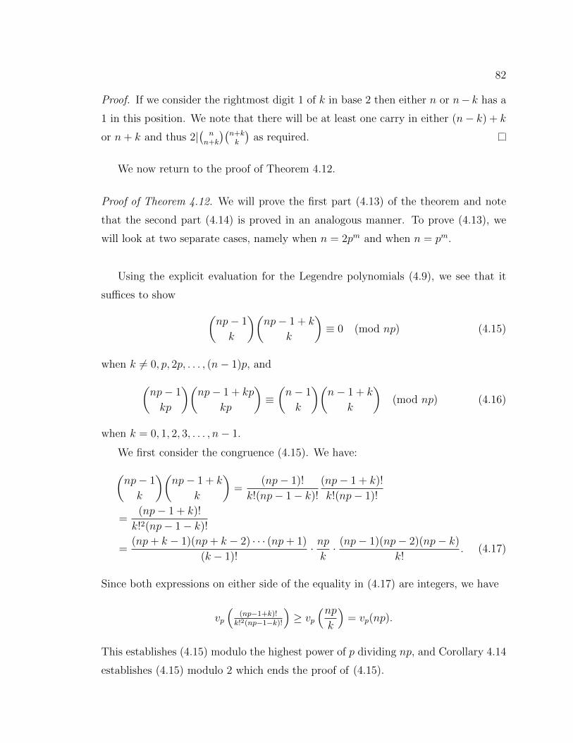
82

Proof. If we consider the rightmost digit 1 of k in base 2 then either n or n− k has a

1 in this position. We note that there will be at least one carry in either (n− k) + k

or n+ k and thus 2|(

nn+k

)(n+kk

)as required.

We now return to the proof of Theorem 4.12.

Proof of Theorem 4.12. We will prove the first part (4.13) of the theorem and note

that the second part (4.14) is proved in an analogous manner. To prove (4.13), we

will look at two separate cases, namely when n = 2pm and when n = pm.

Using the explicit evaluation for the Legendre polynomials (4.9), we see that it

suffices to show (np− 1

k

)(np− 1 + k

k

)≡ 0 (mod np) (4.15)

when k = 0, p, 2p, . . . , (n− 1)p, and(np− 1

kp

)(np− 1 + kp

kp

)≡(n− 1

k

)(n− 1 + k

k

)(mod np) (4.16)

when k = 0, 1, 2, 3, . . . , n− 1.

We first consider the congruence (4.15). We have:(np− 1

k

)(np− 1 + k

k

)=

(np− 1)!

k!(np− 1− k)!

(np− 1 + k)!

k!(np− 1)!

=(np− 1 + k)!

k!2(np− 1− k)!

=(np+ k − 1)(np+ k − 2) · · · (np+ 1)

(k − 1)!· npk

· (np− 1)(np− 2)(np− k)

k!. (4.17)

Since both expressions on either side of the equality in (4.17) are integers, we have

vp

((np−1+k)!

k!2(np−1−k)!

)≥ vp

(npk

)= vp(np).

This establishes (4.15) modulo the highest power of p dividing np, and Corollary 4.14

establishes (4.15) modulo 2 which ends the proof of (4.15).

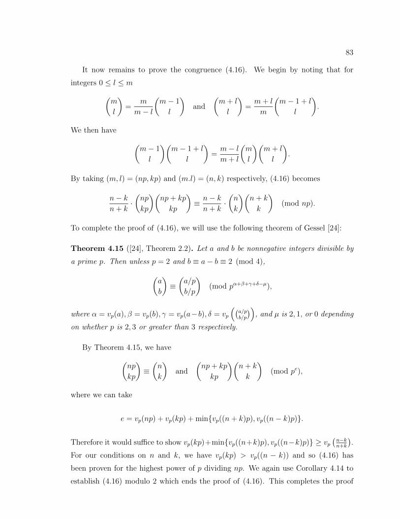
83

It now remains to prove the congruence (4.16). We begin by noting that for

integers 0 ≤ l ≤ m(m

l

)=

m

m− l

(m− 1

l

)and

(m+ l

l

)=

m+ l

m

(m− 1 + l

l

).

We then have (m− 1

l

)(m− 1 + l

l

)=

m− l

m+ l

(m

l

)(m+ l

l

).

By taking (m, l) = (np, kp) and (m.l) = (n, k) respectively, (4.16) becomes

n− k

n+ k·(np

kp

)(np+ kp

kp

)≡ n− k

n+ k·(n

k

)(n+ k

k

)(mod np).

To complete the proof of (4.16), we will use the following theorem of Gessel [24]:

Theorem 4.15 ([24], Theorem 2.2). Let a and b be nonnegative integers divisible by

a prime p. Then unless p = 2 and b ≡ a− b ≡ 2 (mod 4),(a

b

)≡(a/p

b/p

)(mod pα+β+γ+δ−µ),

where α = vp(a), β = vp(b), γ = vp(a−b), δ = vp

((a/pb/p

)), and µ is 2, 1, or 0 depending

on whether p is 2, 3 or greater than 3 respectively.

By Theorem 4.15, we have(np

kp

)≡(n

k

)and

(np+ kp

kp

)(n+ k

k

)(mod pe),

where we can take

e = vp(np) + vp(kp) + min{vp((n+ k)p), vp((n− k)p)}.

Therefore it would suffice to show vp(kp)+min{vp((n+k)p), vp((n−k)p)} ≥ vp(n−kn+k

).

For our conditions on n and k, we have vp(kp) > vp((n − k)) and so (4.16) has

been proven for the highest power of p dividing np. We again use Corollary 4.14 to

establish (4.16) modulo 2 which ends the proof of (4.16). This completes the proof

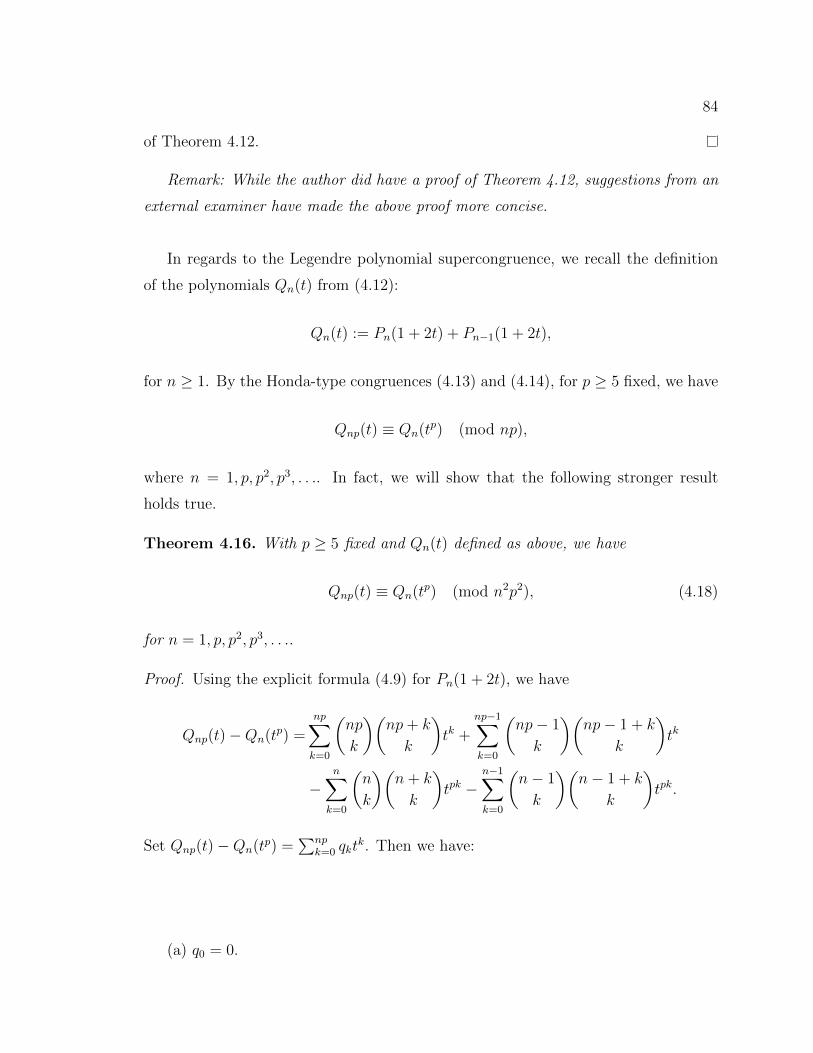
84

of Theorem 4.12.

Remark: While the author did have a proof of Theorem 4.12, suggestions from an

external examiner have made the above proof more concise.

In regards to the Legendre polynomial supercongruence, we recall the definition

of the polynomials Qn(t) from (4.12):

Qn(t) := Pn(1 + 2t) + Pn−1(1 + 2t),

for n ≥ 1. By the Honda-type congruences (4.13) and (4.14), for p ≥ 5 fixed, we have

Qnp(t) ≡ Qn(tp) (mod np),

where n = 1, p, p2, p3, . . .. In fact, we will show that the following stronger result

holds true.

Theorem 4.16. With p ≥ 5 fixed and Qn(t) defined as above, we have

Qnp(t) ≡ Qn(tp) (mod n2p2), (4.18)

for n = 1, p, p2, p3, . . ..

Proof. Using the explicit formula (4.9) for Pn(1 + 2t), we have

Qnp(t)−Qn(tp) =

np∑k=0

(np

k

)(np+ k

k

)tk +

np−1∑k=0

(np− 1

k

)(np− 1 + k

k

)tk

−n∑

k=0

(n

k

)(n+ k

k

)tpk −

n−1∑k=0

(n− 1

k

)(n− 1 + k

k

)tpk.

Set Qnp(t)−Qn(tp) =

∑npk=0 qkt

k. Then we have:

(a) q0 = 0.

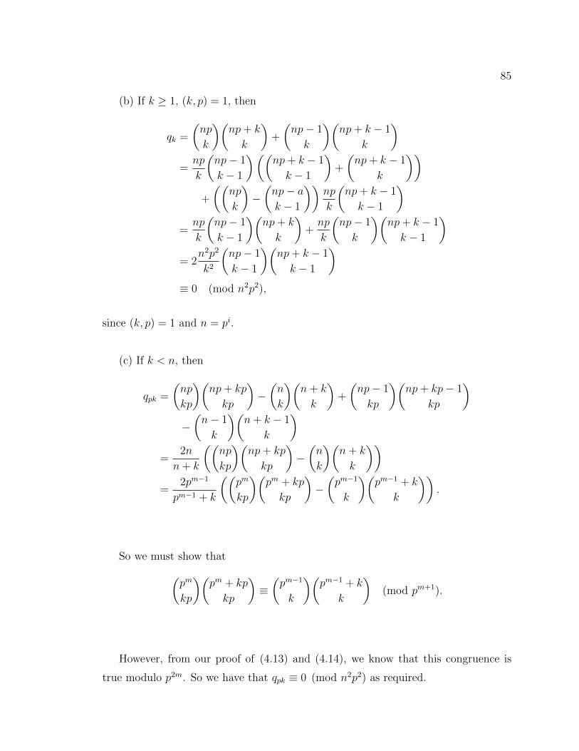
85

(b) If k ≥ 1, (k, p) = 1, then

qk =

(np

k

)(np+ k

k

)+

(np− 1

k

)(np+ k − 1

k

)=

np

k

(np− 1

k − 1

)((np+ k − 1

k − 1

)+

(np+ k − 1

k

))+

((np

k

)−(np− a

k − 1

))np

k

(np+ k − 1

k − 1

)=

np

k

(np− 1

k − 1

)(np+ k

k

)+

np

k

(np− 1

k

)(np+ k − 1

k − 1

)= 2

n2p2

k2

(np− 1

k − 1

)(np+ k − 1

k − 1

)≡ 0 (mod n2p2),

since (k, p) = 1 and n = pi.

(c) If k < n, then

qpk =

(np

kp

)(np+ kp

kp

)−(n

k

)(n+ k

k

)+

(np− 1

kp

)(np+ kp− 1

kp

)−(n− 1

k

)(n+ k − 1

k

)=

2n

n+ k

((np

kp

)(np+ kp

kp

)−(n

k

)(n+ k

k

))=

2pm−1

pm−1 + k

((pm

kp

)(pm + kp

kp

)−(pm−1

k

)(pm−1 + k

k

)).

So we must show that(pm

kp

)(pm + kp

kp

)≡(pm−1

k

)(pm−1 + k

k

)(mod pm+1).

However, from our proof of (4.13) and (4.14), we know that this congruence is

true modulo p2m. So we have that qpk ≡ 0 (mod n2p2) as required.

86

(d) We lastly consider qnp, namely

qnp =

(2np

np

)−(2n

n

)=

(2pm

pm

)−(2pm−1

pm−1

).

To prove that qpm ≡ 0 (mod p2m) as required, we will invoke the following theorem

of Jacobsthal which can be found in [26].

Theorem 4.17 (Jacobsthal). For any integers ν > µ > 0 and prime p ≥ 5,(νpµp

)(νµ

) ≡ 1 (mod pq),

where q is the power of p dividing p3νµ(ν − µ).

In our case, ν = 2pm−1, µ = pm−1, and q = 3m. This gives us the congruence

qnp ≡ 0 (mod p3m) which is actually stronger than the congruence we required. This

completes the proof of Theorem 4.16

We finish this section by clarifying that Theorem 4.12, and by extension Theorem

4.16, are not new results but rather new arguments for (4.10) and (4.11) considered

over the integers.

4.5 Other Polynomials

Given that Legendre polynomials are special cases of Jacobi polynomials, our work

in Section 2.4 leads to the question whether Honda-type congruences also hold for

Jacobi polynomials in general. That is, are there congruences of the form

P (α,β)n (1 + 2tp) ≡ P (α,β)

np (1 + 2t) (mod np)?

Supported by computer experimentation, it appears that, with the exception of

α = β = 0 (the Legendre case) and α = β = −12, no such congruences exist. There is

an issue with the coefficients of the polynomials not being invertible modulo np.

87

The case α = β = −12is the case of the Chebyshev polynomials of the first kind.

We will use the following explicit formula for the Chebyshev polynomials of the first

kind which can be found in [52]:

Tn(x) =n

2

⌊n2⌋∑

k=0

(−1)k(n− k − 1)!

k!(n− 2k)!(2x)n−2k.

For a fixed prime p, we have the following congruence:

Theorem 4.18. For any prime p, we have

Tnp(x) ≡ Tn(xp) (mod np),

where n = 2ipj, i, j ≥ 0.

Proof. We need to show that

np

2

⌊np2⌋∑

k=0

(−1)k(np− k − 1)!

k!(np− 2k)!(2x)np−2k ≡ n

2

⌊n2⌋∑

k=0

(−1)k(n− k − 1)!

k!(n− 2k)!(2xp)n−2k (mod np).

We are done if we can show that the following two congruences hold for k = 0, 1, 2, . . . :

np

22np−2k(−1)k

(np− k − 1)!

k!(np− 2k)!≡ 0 (mod np), k = 0, p, 2p, . . . , (4.19)

np

22np−2k(−1)k

(np− k − 1)!

k!(np− 2k)!≡ n

22n−2k(−1)k

(n− k − 1)!

k!(n− 2k)!(mod np), all other k.

(4.20)

We begin by showing the first congruence (4.19):

np

22np−2k(−1)k

(np− k − 1)!

k!(np− 2k)!=

np

22np−2k(−1)k

(np− k − 1) · · · (np− 2k + 1)

k!

≡ 0 (mod np)

since k = mp for m ∈ Z and n = 2ip, so the factor of np out front will not cancel.

We now prove the second congruence (4.20). We begin by simplifying the left-hand

88

side of (4.20):

np

22np−2k(−1)kp

(np− k − 1)!

k!(np− 2k)!

=2ipj+1

22np−2kp(−1)kp

(2ipj+1 − kp− 1) · · · (2ipj+1 − 2kp+ 1)

(kp)!

= 2np−2kp+i−1pj+1(−1)kp(2ipj+1 − kp− 1) · · · (2ipj+1 − 2kp+ 1)

(kp)!.

For simplifying the right-hand side of (4.20), we note

n

22n−2k(−1)k

(n− k − 1)!

k!(n− 2k)!=

2ipj

22n−2k(−1)k

(2ipj − k − 1) · · · (2ipj − 2k + 1)

k!

= 2n−2k+i−1pj(−1)k(2ipj − k − 1) · · · (2ipj − 2k + 1)

k!.

It is clear that modulo 2i, both the left-hand side and the right-hand side of (4.20) are

congruent to 0. Now we only need to consider both sides modulo pj+1. Furthermore,

since both sides have a factor of pj, we will divide it out and consider everything

modulo p. We again begin with the left-hand side of (4.20):

(2p)n−2k2i−1p(−1)kp(2ipj+1 − kp− 1) · · · (2ipj+1 − 2kp+ 1)

(kp)!

≡ 2n−2k2i−1 (−1)kp

k

(−kp− 1) · · · (−2kp+ 1)

(kp− 1)!(mod p)

≡ 2n−2k2i−1 (−1)k

k(−1)kp−1

(2kp− 1

kp

)(mod p)

≡ 2n−2k+i−1 (−1)2k−1

k

(2kp− 1

kp

)(mod p).

89

We now look at the right-hand side of (4.20):

2n−2k2i−1(−1)k(2ipj − k − 1) · · · (2ipj − 2k + 1)

k!

≡ 2n−2k2i−1 (−1)k

k

(−k − 1) · · · (−2k + 1)

(k − 1)!(mod p)

≡ 2n−2k2i−1 (−1)k

k(−1)k−1

(2k − 1

k

)(mod p)

≡ 2n−2k+i−1 (−1)2k−1

k

(2k − 1

k

)(mod p).

To complete the proof and show that the two sides are indeed congruent modulo p,

we use the following theorem of Lucas which can be found in [26]:

Theorem 4.19 (Lucas). Let m0 and n0 be the least non-negative residues of m and

n modulo p, respectively. Then(n

m

)≡(⌊n

p⌋

⌊mp⌋

)(n0

m0

)(mod p).

Using this theorem, we have(2kp−1kp

)≡(2k−1k

)(mod p) and the proof of Theorem

4.18 is complete.

We now illustrate Theorem 4.18 with an example:

Example 4.20. Let us set p = 3, i = 1, and j = 1. Then n = 2 · 3 = 6 and we

calculate

Tnp(x) = T18(x) = 131072x18 − 589824x16 + 1105920x14 − 1118208x12 + 658944x10

− 228096x8 + 44352x6 − 4320x4 + 162x2 − 1,

Tn(xp) = T6(x

3) = 32x18 − 48x12 + 18x6 − 1.

Reducing modulo np = 6 · 3 = 18, we get

T18(x) = 14x18 + 6x12 + 17 (mod 18)

90

and

T6(x3) = 14x18 + 6x12 + 17 (mod 18),

as expected.

The Chebyshev polynomials of the second kind, Ux(x), can be expressed in terms

of the Chebyshev polynomials of the first kind, Tn(x). For more information regarding

the relationship between Tn(x) and Un(x) as well as an explicit formula for Un(x) the

reader is referred to Theorem A.6 in the appendices, and to [52]. As an immediate

consequence of Theorem 4.18 we have the following two corollaries:

Corollary 4.21. For p an odd prime, we have

Unp(x)− Unp−2(x) ≡ Un(xp)− Un−2(x

p) (mod np)

for n = 2ipj, i, j ≥ 0.

Corollary 4.22. For p = 2, we have

U2k+1(x)− U2k+1−2(x) ≡ U2k(x2)− U2k−2(x

2) (mod 2k+1)

for k ≥ 0.

4.6 Comments

Further commentary on Theorem 4.19 as well as a generalized version of Theorem

4.19 may be found in [42].

We continued to do some Maple experimentation with more Jacobi polynomials

and Hermite polynomials. While no results analogous to Honda’s congruences (4.13)

and (4.14) were found in these cases, it has led us to investigate other related results

for these polynomials and make the following observations.

There are some differences between the work of Robert and Zuber (Theorem

4.11) and our work that are worth mentioning. Despite being similar to the results

91

in the paper [53], our results are obtained without the use of p-adic numbers. The

congruences in [53] are modulo a multiple of Zp while ours are over Z. However, thecongruences in [53] hold for any value of n, while ours only hold for specific values of n.

We have considered the difference of the two sides of Honda’s congruences (4.13),

(4.14) and tried to see if we get recognizable polynomial sequences when they do not

equal 0. No recognizable sequences or patterns were found.

We have also considered the divisibility of the denominators of the coefficients of

these Jacobi polynomials. Since they are not invertible, they are sharing a non-trivial

factor with np. The power of this factor showing up in the denominator of each Jacobi

polynomial forms a non-monotonic sequence that has relatively large values for some

indices in the sequence.

The congruences for Qn(t) found in Theorem 4.16 no longer hold in the cases

n = 2pm . The problem arises modulo 2 and modulo 22. We will demonstrate this

with an example.

Example 4.23. If we take p = 7 and n = 1, we get:

Q7(t) = 2t7 + 2 (mod 72) Q1(t) = 2t+ 2 (mod 72)

and Theorem 4.16 holds as desired. However,

Q7(t) = 2t7 + 2 (mod 22) Q1(t) = 2t+ 2 (mod 22)

and here Theorem 4.16 fails to hold since 2t7 + 2 ≡ 2t+ 2 (mod 22).

For the Legendre polynomials, unfortunately, the parallel ends here because a

congruence of the form

Tn−1(xp) ≡ Tnp−1(x) (mod np)

does not hold. This means that we cannot define the analogue of Qn(x) from the

Legendre case.

92

The congruence in Theorem 4.18 we found resembles a result by Dilcher and

Chamberland [14, Theorem 2.1], specifically regarding the values of n for which it

holds. Maybe there is a connection deeper than just “shape”.

No such congruence was found for the Chebyshev polynomials of the second kind,

but given the close relationship they share with those of the first kind, I believe that

there would be an analogue of some sort for the polynomials of the second kind.

Chapter 5

Conclusion

We begin this chapter with final comments on some of the results in the thesis.

This is followed by natural questions related to the work in Chapters 2–4 and by

some remarks on possible further work. Any background material referenced in the

thesis as well as a few elementary examples of the objects studied are collected in the

appendices.

5.1 Comments

5.1.1 The case a = 0 in Chapter 3

Unless explicitly stated otherwise, the results presented in Chapter 3 concerning

the polynomials fa,cn (x), ga,cn (x), ha,c

n (x), and ka,cn (x) also apply to the polynomials

f(x), g(x), h(x), and k(x) studied by Harrington in [28] if you take a = 0.

5.1.2 Height of Jn,H(x)

If P (x) = amxm + am−1x

m−1 + . . . + a1x + a0 is a polynomial of degree m, then the

height of P (x) is defined as max{ai}mi=0. For a given integer n, we wondered for which

subgroup H ≤ (Z/nZ)× did Jn,H(x) have the largest height. This is a question that

is of interest for all of the varying special cases of n studied in Chapter 2. Although

not true in general, it appears to be the case that the polynomial Jn,{1,−1}(x) is the

one with largest height in each family for certain cases on the integer n.

5.1.3 Potential Applications

In their joint paper [33], Joyner and Shaska discuss the applications of self-inverse

or self-reciprocal polynomials to coding theory and reduction theory. They credit

the behaviour of the roots of self-reciprocal polynomials and their location in the

complex plane for their utility in the subject. It would be of interest to study the

93

94

potential relationship between the self-reciprocal polynomials of the form Jn,H(x) for

some integers n and subgroup H ≤ (Z/nZ)× and such applications.

5.2 Further Directions

While studying congruences of the form of (4.13),(4.14) in Chapter 4, differences of

Jacobi polynomials were considered modulo powers of an odd prime p. There seem

to be “spikes” of divisibility as the integer n ranges with no currently discernible

pattern. Studying the divisibility of these differences may lead to new congruences

for Jacobi polynomials.

In Chapter 4, we mentioned that the authors of [13] considered the base-5 ex-

pansion of the primes such that 5p satisfied (2.2) but no such characterization was

found. Through numerical experimentation, an interesting observation was made:

taking the primes p such that 5p satisfied (4.6) and plugging them into the function

f(x) = 5x + 4 resulted in f(p) not being prime or f(p) remaining prime for an odd

number of iterations of f(x).

Although they were not applied in this thesis, it is of interest to revisit the ap-

proach of Robert and Zuber [53] in an attempt to apply those methods to the more

general Jacobi polynomials in hope of obtaining modulo p congruences or congruences

in Zp for primes p.

In Chapter 3, we proved a result regarding the discriminants of the polynomials

studied in [28] by Harrington and their variation introduced in Chapter 3. We would

like to study these discriminants in more depth, as well as study the resultants of

pairs of these polynomials.

Despite not being able to get a direct analogue to Theorem 3.1 in this thesis,

that is not to say it is an impossible task. We would like to investigate this matter

further and potentially classify more examples of reducible and/or irreducible families

of polynomials.

95

In Chapter 2 we studied the coefficients of Cyclotomic Subgroup-Polynomials

Jn,H(x) for fixed orders of the subgroup H. Namely, the cases discussed were |H| =1, 2, 3, and 4. We would like to study the cases Jn,H(x) when H is of order 5 and

higher.

At the very beginning of Chapter 2 we restricted our attention to integers n that

resulted in cyclic groups (Z/nZ)×. This choice was made because of the nice struc-

ture of cyclic groups and the nice structure of their subgroups. We would like to

study the set of Cyclotomic Subgroup-Polynomials for integers n when (Z/nZ)× is

not necessarily a cyclic group.

While we were not able to find the limiting curve for the roots of the Galois

Subgroup-Polynomials, there does seem to be some pattern in the behaviour of these

roots. We would like to study these roots in more detail in attempt to find a limiting

curve or some long-term behaviour.

Theorem 2.65 can be considered the “order 2” analogue of Apostol’s famous re-

sult on the resultant of cyclotomic polynomials. In Chapter 2 we mention that we

couldn’t find evidence of an “order 3” analogue of Apostol’s result; we would like to

study this further in hopes of finding an “order 3” analogue or explaining the non-

existence of one. It is also of interest to study the discriminants of the Cyclotomic

Subgroup-Polynomials for different values of the positive integers n, a, and c.

As mentioned in Chapter 2, if the integer n is free of any square prime factors then

Jn,H(x) will be irreducible for all subgroups H ≤ (Z/nZ)×. That isn’t to say that it

is not possible for Jn,H(x) to be irreducible when n has a squared prime factor. An

area of interest would be to try to enumerate the number of irreducible polynomials

for any given integer n.

Appendices

96

Appendix A

Some Mathematical Background

Let x be an indeterminate and R a commutative ring with unity. The formal sum,

anxn + an−1x

n−1 + . . . + a1x + a0, with n ≥ 0 and ai ∈ R for each i is called a poly-

nomial in x with coefficients in R. Given an = 0, we say that the polynomial is of

degree n and we call an the leading coefficient. In the special case an = 1, we refer to

the polynomial as a monic polynomial of degree n. The set of all such polynomials

forms the ring of polynomials in x with coefficients in R, denoted R[x], along with

the two familiar operation of addition and multiplication.

Definition A.1. Let n be a positive integer, K a field such that char(K) does not

divide n, and F a cyclotomic extension of order n of K. The nth cyclotomic poly-

nomial over K is the monic polynomial Φn(x) = (x − ζ1)(x − ζ2) · · · (x − ζr) where

ζ1, . . . , ζr are all the distinct primitive nth roots of unity in F .

A.0.1 Properties of the Cyclotomic Polynomials

Φn(x) =∏d|n

(xd − 1)µ(nd), (A.1)

where µ is the Mobius function. Special cases:

Φp(x) =

p−1∑k=0

xk = 1 + x+ x2 + . . .+ xp−2 + xp−1. (A.2)

Φ2p(x) =

p−1∑k=0

(−x)k = 1− x+ x2 − x3 + . . .− xp−2 + xp−1. (A.3)

97

98

In the case n = pmr, with (p, r) = 1, we have

Φn(x) = Φpr(xpm−1

). (A.4)

A.0.2 Properties of Binomial Coefficients

(n

k

)=

n!

k!(n− k)!.

(n

k

)=

(n− 1

k

)+

(n− 1

k − 1

).

(x+ y)n =n∑

k=0

(n

k

)xn−kyk.

A.0.3 Chebyshev Polynomials

Definition A.2. The Chebyshev Polynomials of the first kind are defined by the

recurrence relation

T0(x) = 1,

T1(x) = x,

Tn+1(x) = 2xTn(x)− Tn−1(x), n ≥ 2.

Definition A.3. The Chebyshev Polynomials of the second kind are defined by the

recurrence relation

U0(x) = 1,

U1(x) = 2x,

Un+1(x) = 2xUn(x)− Un−1(x), n ≥ 2.

99

Lemma A.4. The Chebyshev polynomials have the following generating functions:

∞∑n=0

Tn(x)tn =

1− tx

1− 2tx+ t2, (A.5)

∞∑n=0

Un(x)tn =

1

1− 2tx+ t2. (A.6)

Lemma A.5. The Chebyshev polynomials satisfy the following identities:

Tn(cos(θ)) = cos(nθ), (A.7)

Un(cos(θ)) =sin((n+ 1)θ)

sin(θ). (A.8)

Theorem A.6. The Chebyshev polynomials of the second kind have the following

explicit expressions:

Un(x) =(x+

√x2 − 1)n+1 − (x−

√x2 − 1)n+1

2√x2 − 1

, (A.9)

=

⌊n2⌋∑

k=0

(n+ 1

2k + 1

)(x2 − 1)kxn−2k, (A.10)

= xn

⌊n2⌋∑

k=0

(n+ 1

2k + 1

)(1− x2)kxk, (A.11)

=

⌊n2⌋∑

k=0

(2k − (n+ 1)

k

)(2x)n−2k, n > 0, (A.12)

=

⌊n2⌋∑

k=0

(−1)k(n− k

k

)(2x)n−2k, n > 0, (A.13)

=n∑

k=0

(−2)k(n+ k + 1)!

(n− k)!(2k + 1)!(1− x)k, n > 0. (A.14)

Lemma A.7. The Chebyshev polynomials satisfy the following identities:

Tn(x) =1

2(Un(x)− Un−2(x)) , (A.15)

2xUn(1− 2x2) = (−1)nU2n+1(x). (A.16)

100

A.0.4 General Polynomial Results

Suppose we have the following polynomial with integer coefficients:

P (x) = anxn + an−1x

n−1 + an−2xn−2 + . . .+ a1x+ a0.

We begin with some important irreducibility criteria.

Theorem A.8 (Eisenstein Criterion). If there exists a prime number p such that the

following three conditions all apply:

(i) p divides each ai for i = n,

(ii) p does not divide an,

(iii) p2 does not divide a0,

then P (x) is irreducible over the rationals.

Definition A.9. Let P (x) be as above with ai ∈ K for K a local field with discrete

valuation and with a0an = 0. Then the Newton polygon of P (x) is defined to be the

lower convex hull of the set of points {Qi = (i, vK(ai)}, ignoring the points where

ai = 0.

Theorem A.10 (Schonemann’s Criterion). Suppose that a polynomial f(x) ∈ Z[x]has the form f(x) = ϕ(x)e+pM(x), where p is a prime number, ϕ(x) is an irreducible

polynomial modulo p, and M(x) is a polynomial relatively prime to ϕ(x) modulo p,

with deg(M) < deg(f). Then f is irreducible over Q.

Definition A.11. Let p be a fixed prime, and let f(x) =∑n

i=0Aixi be a polynomial

with integer coefficients such that A0An = 0. Let us represent the nonzero coefficients

of f in the form Ai = aipαi, where ai is an integer not divisible by p. To every

nonzero coefficient aipαi we assign a point in the plane with coordinated (i, αi). These

points give rise to the Newton Diagram of the polynomial f (corresponding to p).

The construction of the diagram is as follows. Let P0 = (0, α0) and P1 = (i1, αi1),

where i1 is the largest integer for which there are no points (i, αi) below the line P0P1.

Further let P2 = (i2, αi2), where I2 is the largest integer for which there are no points

(i, αi) below the line P1P2, etc. The very last segment is of the form Pr−1Pr where

101

Pr = (n, αn). If some segments of the broken line P0, . . . , Pr pass through points with

integer coordinates, then such points will be also considered as vertices of the broken

line.

Theorem A.12 (Dumas). Let f = gh, where f, g, and h are polynomials with integer

coefficients. Then the system of vectors of the segments for f is the union of the

systems of vectors of the segments for g and h (provided that p is the same for all

polynomials).

Corollary A.13. If, for a prime p, the Newton diagram for f consists of precisely

one segment, i.e., consists of a segment containing no points with integer coefficients,

then f is irreducible.

Lemma A.14. The Legendre polynomials, Pn(ζ), can be defined as coefficients of the

generating function

1√1− 2ζx+ x2

=∞∑n=0

Pn(ζ)xn.

Carrying out the substitution ζ = 1 + 2t, we obtain the following explicit formula for

Pn(1 + 2t)

Pn(1 + 2t) =n∑

k=0

(n

k

)(n+ k

k

)tk.

Theorem A.15 (Viete’s Formulas). Given the polynomial f(x) = anxn+an−1x

n−1+

. . .+ a1x+ a0, with an = 0, with its (not necessarily distinct) zeros x1, x2, . . . , xn, we

have the following formulas:⎧⎪⎪⎪⎪⎪⎪⎪⎨⎪⎪⎪⎪⎪⎪⎪⎩

x1 + x2 + . . .+ xn−1 + xn = −an−1

an,

(x1x2 + x1x3 + . . .+ x1xn) + (x2x3 + x2x4 + . . .+ x2xn) + . . .+ xn−1xn = an−2

an,

...

x1x2x3 · · ·xn = (−1)n a0an.

102

A.0.5 Algebra Results

Theorem A.16. If R is a unique factorization domain, then R[x] is a unique fac-

torization domain.

Theorem A.17. A finite field F with n elements exists if and only if n = pk for some

odd prime p and some non-negative integer k. Moreover, this field is unique up to

isomorphism.

Theorem A.18 (Structure Theorem for Finite Abelian Groups). Every finite Abelian

group is isomorphic to a direct product of cyclic groups of orders that are powers of

prime numbers. That is, if G is a finite Abelian group, then

G ∼= Zpk11× Z

pk22× · · · × Zpknn

,

where |G| = pk11 pk22 · · · pknn .

A.0.6 Number Theory Results

Theorem A.19 (Wilson’s Theorem). For an odd prime, p,

(p− 1)! ≡ −1 (mod p).

Theorem A.20. There exists a primitive root modulo m if and only if m = 1, 2, 4, pα,

and 2pα in which p is an odd prime and α is a natural number.

Theorem A.21. For a positive integer n, we have

µ(n) =n∑

k=1(k,n)=1

exp

(2πik

n

).

Appendix B

SAGE Code

The computer algebra system SAGE was used to generate a list of all subgroups of

the group of multiplicative integers (Z/nZ)× for a given integer n. The computer

algebra system Maple is capable of doing these calculations as well but SAGE was

preferred in this case due to its speed.

The author used some advice and suggestions from different discussion posts found

at the website https://ask.sagemath.org/questions/ .

Attached is a small example of how SAGE was used.

103

Xfa�;2 �TT2M/BtXb�;2rb

62#`m�`v Rk- kyRN

/2 7 H B b i n 2 H i b U:V ,2tTb 4 ( `�M;2 U ; X Km H i B T H B + � i B p 2nQ`/2 ` U V V 7 Q ` ; BM :)`2 im`M ( T`Q/ U ;�2 7 Q ` ; - 2 BM x BT U:- 2tT V V 7 Q ` 2tT BM \

*�`i2b B�MS`Q/m+i U 2tTb V )

_ 4 AM i 2 ; 2 ` b Uj V c K�TU H B b in 2 H i b - _X KmH i BT H B +� i Bp2nbm#;`QmTb U V V((R- k)- (R))

_ 4 AM i 2 ; 2 ` b U9 V c K�TU H B b in 2 H i b - _X KmH i BT H B +� i Bp2nbm#;`QmTb U V V((R- j)- (R))

_ 4 AM i 2 ; 2 ` b U8 V c K�TU H B b in 2 H i b - _X KmH i BT H B +� i Bp2nbm#;`QmTb U V V((R- k- 9- j)- (R- 9)- (R))

_ 4 AM i 2 ; 2 ` b Ue V c K�TU H B b in 2 H i b - _X KmH i BT H B +� i Bp2nbm#;`QmTb U V V((R- 8)- (R))

_ 4 AM i 2 ; 2 ` b Ud V c K�TU H B b in 2 H i b - _X KmH i BT H B +� i Bp2nbm#;`QmTb U V V((R- j- k- e- 9- 8)- (R- k- 9)- (R- e)- (R))

R

Appendix C

Maple Code

The computer algebra systemMaple was used to generate lists of the Galois Subgroup-

Polynomials for a given integer n. The computer algebra system SAGE is capable

of doing these calculations as well but Maple was preferred in this case due to its speed.

The author used some advice and suggestions from different discussion posts found

at the website https://www.mapleprimes.com, and modified some of the functions

found in found in the following master’s thesis to suit this task:

Cooper, III, Thomas Edmond, “Using the Maple Computer Algebra System as a

Tool for Studying Group Theory.” Master’s Thesis, University of Tennessee, 2002.

Attached is a small example of how Maple was used.

105

> >

> >

> >

> > > >

> >

> >

> >

> >

> >

> >

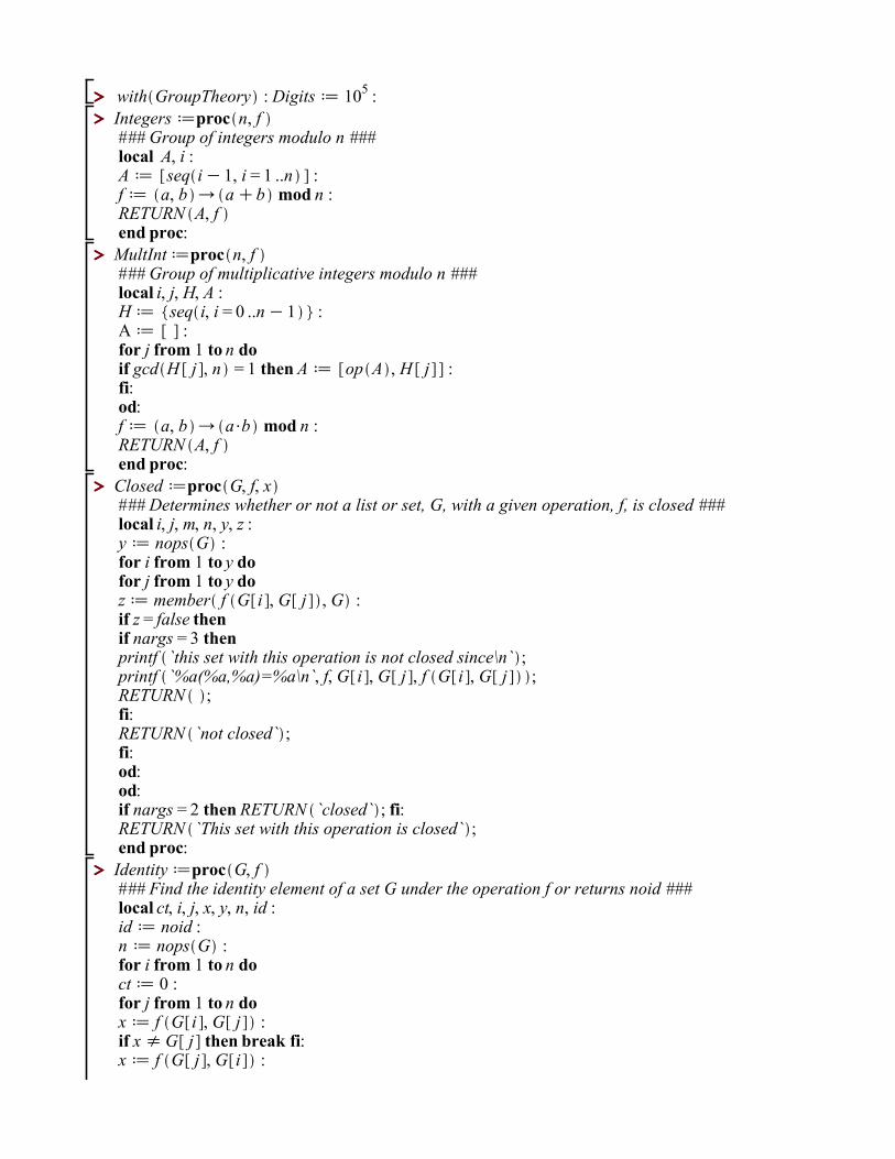
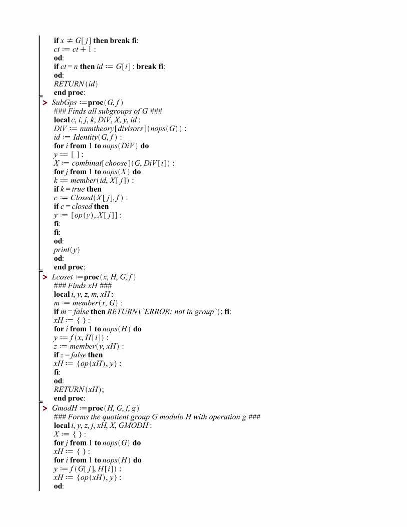
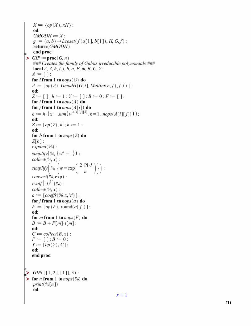
(1)(1)

> >

> >

> >

> >

> >

> >

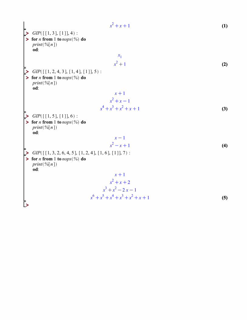
(3)(3)

> >

(1)(1)

> >

> >

> >

> >

(4)(4)

(5)(5)

> >

> >

(2)(2)

> >

x1

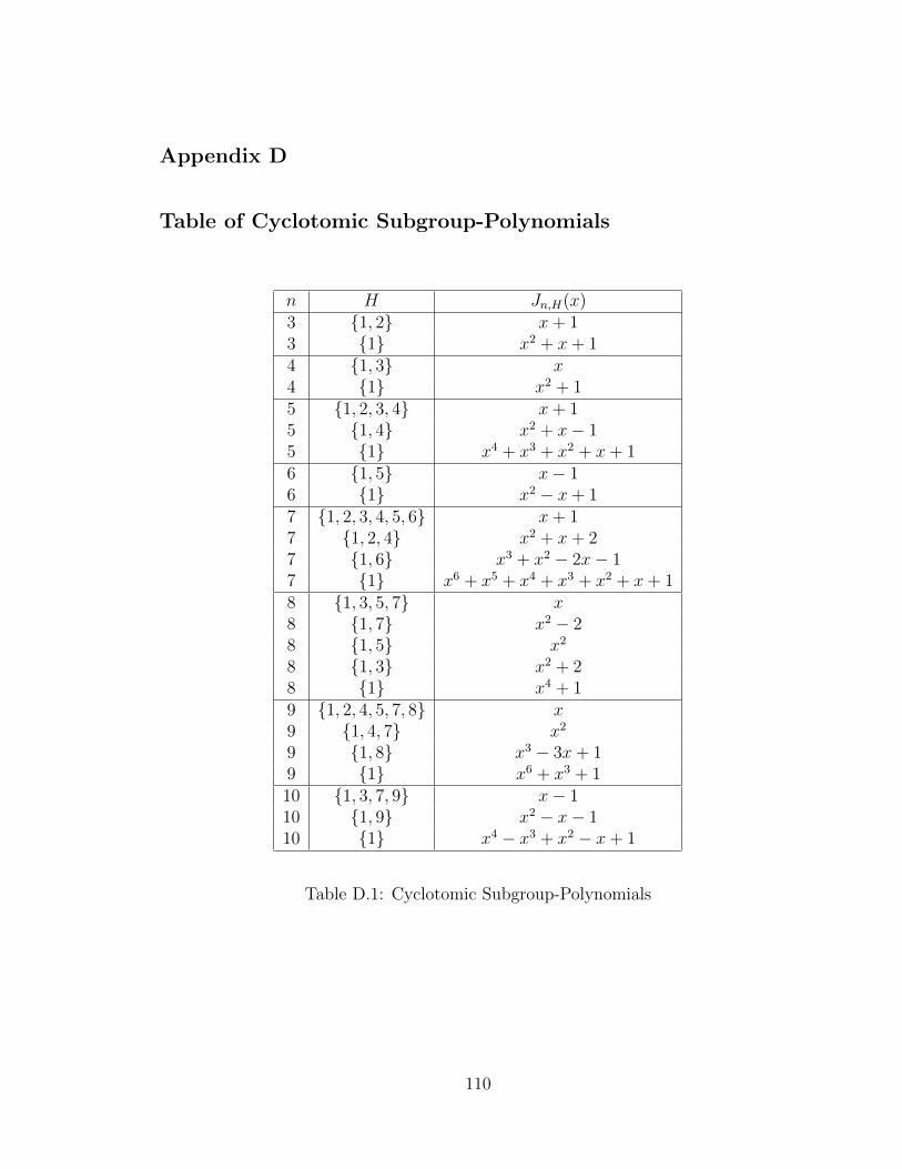
Appendix D

Table of Cyclotomic Subgroup-Polynomials

n H Jn,H(x)3 {1, 2} x+ 13 {1} x2 + x+ 14 {1, 3} x4 {1} x2 + 15 {1, 2, 3, 4} x+ 15 {1, 4} x2 + x− 15 {1} x4 + x3 + x2 + x+ 16 {1, 5} x− 16 {1} x2 − x+ 17 {1, 2, 3, 4, 5, 6} x+ 17 {1, 2, 4} x2 + x+ 27 {1, 6} x3 + x2 − 2x− 17 {1} x6 + x5 + x4 + x3 + x2 + x+ 18 {1, 3, 5, 7} x8 {1, 7} x2 − 28 {1, 5} x2

8 {1, 3} x2 + 28 {1} x4 + 19 {1, 2, 4, 5, 7, 8} x9 {1, 4, 7} x2

9 {1, 8} x3 − 3x+ 19 {1} x6 + x3 + 110 {1, 3, 7, 9} x− 110 {1, 9} x2 − x− 110 {1} x4 − x3 + x2 − x+ 1

Table D.1: Cyclotomic Subgroup-Polynomials

110

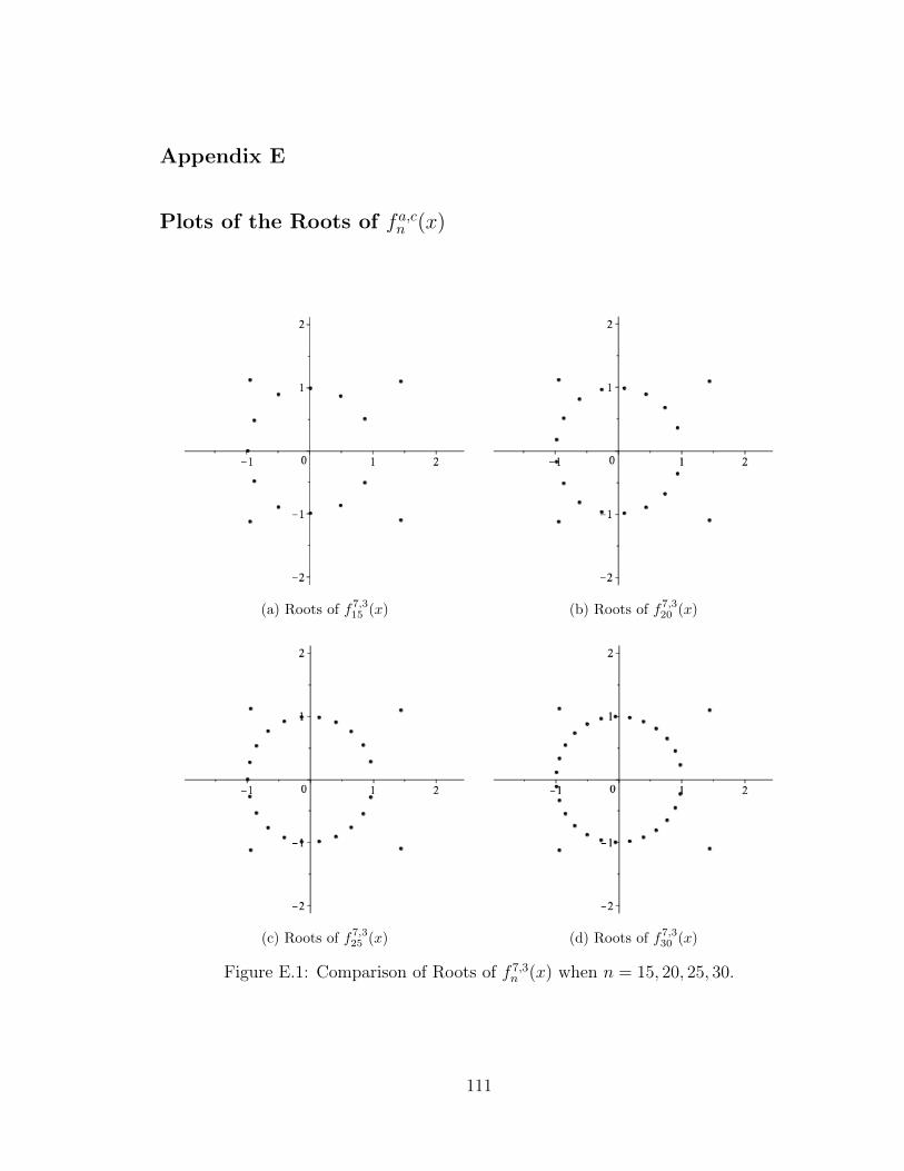
Appendix E

Plots of the Roots of fa,cn (x)

(a) Roots of f7,315 (x) (b) Roots of f7,3

20 (x)

(c) Roots of f7,325 (x) (d) Roots of f7,3

30 (x)

Figure E.1: Comparison of Roots of f 7,3n (x) when n = 15, 20, 25, 30.

111

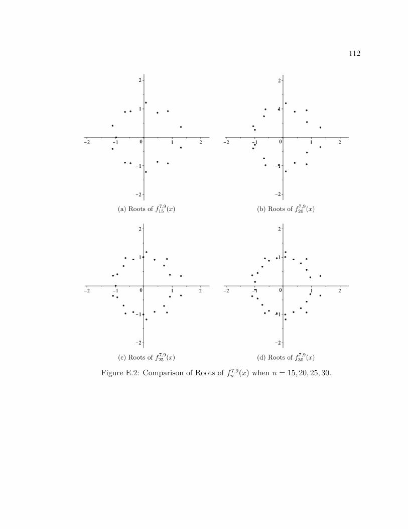
112

(a) Roots of f7,915 (x) (b) Roots of f7,9

20 (x)

(c) Roots of f7,925 (x) (d) Roots of f7,9

30 (x)

Figure E.2: Comparison of Roots of f 7,9n (x) when n = 15, 20, 25, 30.

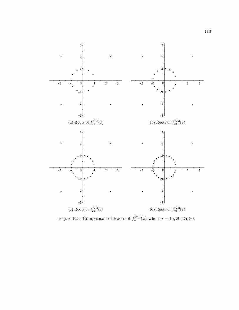
113

(a) Roots of f77,315 (x) (b) Roots of f77,3

20 (x)

(c) Roots of f77,325 (x) (d) Roots of f77,3

30 (x)

Figure E.3: Comparison of Roots of f 77,3n (x) when n = 15, 20, 25, 30.

Bibliography

[1] Dorin Andrica and Ovidiu Bagdasar. On some results concerning the polygonalpolynomials. Carpathian Journal of Mathematics., 2019.

[2] Dorin Andrica and Ovidiu Bagdisar. Some remarks on a general family of com-plex polynomials. Submitted for Publication, 2018.

[3] Tom M. Apostol. Resultants of cyclotomic polynomials. Proc. Amer. Math. Soc.,24:457–462, 1970.

[4] D. F. Bailey. More binomial coefficient congruences. Fibonacci Quart., 30(2):121–125, 1992.

[5] E. J. Barbeau. Polynomials. Problem Books in Mathematics. Springer NewYork, 2003.

[6] Serban Barcanescu. The coefficients of the period polynomials. arXiv e-prints,page arXiv:1402.3833, Feb 2014.

[7] Bruce C. Berndt, R. J. Evans, and K. S. Williams. Gauss and Jacobi sums.Canadian Mathematical Society series of monographs and advanced texts. Wiley,1998.

[8] Scott Beslin and Valerio De Angelis. The minimal polynomials of sin (2πp) and

cos (2πp). Math. Mag., 77(2):146–149, 2004.

[9] F. Beukers. Some congruences for the Apery numbers. J. Number Theory,21(2):141–155, 1985.

[10] F. Rudolf Beyl. Cyclic subgroups of the prime residue group. Amer. Math.Monthly, 84(1):46–48, 1977.

[11] P. Borwein and T. Erdelyi. Polynomials and Polynomial Inequalities. GraduateTexts in Mathematics. Springer New York, 1995.

[12] Antonio Cafure and Eda Cesaratto. Irreducibility criteria for reciprocal polyno-mials and applications. Amer. Math. Monthly, 124(1):37–53, 2017.

[13] Marc Chamberland and Karl Dilcher. Divisibility properties of a class of binomialsums. J. Number Theory, 120(2):349–371, 2006.

[14] Marc Chamberland and Karl Dilcher. A binomial sum related to Wolstenholme’stheorem. J. Number Theory, 129(11):2659–2672, 2009.

114

115

[15] H. Cohen. A Course in Computational Algebraic Number Theory. GraduateTexts in Mathematics. Springer Berlin Heidelberg, 2013.

[16] Matthijs Coster. Supercongruences. PhD thesis, Universiteit Leiden, 1988.

[17] David A. Cox. Primes of the Form x2 + ny2. Pure and Applied Mathematics(Hoboken). John Wiley & Sons, Inc., Hoboken, NJ, second edition, 2013. Fermat,class field theory, and complex multiplication.

[18] Gregory Dresden. Resultants of cyclotomic polynomials. Rocky Mountain J.Math., 42(5):1461–1469, 2012.

[19] Paulius Drungilas, Jonas Jankauskas, and Jonas Siurys. On Newman and Lit-tlewood multiples of Borwein polynomials. arXiv e-prints, Sep 2016.

[20] D.S. Dummit and R.M. Foote. Abstract Algebra. Wiley, 2004.

[21] A.W.F. Edwards. Pascal’s Arithmetical Triangle: The Story of a MathematicalIdea. Johns Hopkins Paperback. Johns Hopkins University Press, 2002.

[22] Harriet Fell. The geometry of zeros of trinomial equations. Rendiconti del CircoloMatematico di Palermo, 29(2):303–336, May 1980.

[23] Michael Filaseta and Ikhalfani Solan. An extension of a theorem of Ljunggren.Math. Scand., 84(1):5–10, 1999.

[24] Ira M. Gessel. Some congruences for generalized Euler numbers. Canad. J.Math., 35(4):687–709, 1983.

[25] T. Gowers, J. Barrow-Green, and I. Leader. The Princeton Companion to Math-ematics. Princeton University Press, 2010.

[26] Andrew Granville. Arithmetic properties of binomial coefficients. I. Binomialcoefficients modulo prime powers. In Organic mathematics (Burnaby, BC, 1995),volume 20 of CMS Conf. Proc., pages 253–276. Amer. Math. Soc., Providence,RI, 1997.

[27] E. R. Hansen. A Table of Series and Products. Prentice-Hall series in automaticcomputation. Prentice-Hall, 1975.

[28] Joshua Harrington. On the factorization of the trinomials xn + cxn−1 + d. Int.J. Number Theory, 8(6):1513–1518, 2012.

[29] Taira Honda. Two congruence properties of Legendre polynomials. Osaka J.Math., 13(1):131–133, 1976.

[30] T. W. Hungerford. Algebra. Graduate Texts in Mathematics. Springer New York,2003.

116

[31] Saud Hussein. New conjecture related to a conjecture of McIntosh. arXiv e-prints, Feb 2018.

[32] Svante Janson. Resultant and discriminant of polynomials. 2007.

[33] David Joyner and Tony Shaska. Self-inversive polynomials, curves, and codes.arXiv e-prints, Jun 2016.

[34] E. E. Kummer. Uber die Erganzungssatze zu den allgemeinen Re-ciprocitatsgesetzen. J. Reine Angew. Math., 44:93–146, 1852.

[35] Miyeon Kwon, Ji-Eun Lee, and Ki-Suk Lee. Galois irreducible polynomials.Commun. Korean Math. Soc., 32(1):1–6, 2017.

[36] T. Y. Lam and K. H. Leung. On vanishing sums of roots of unity. J. Algebra,224(1):91–109, 2000.

[37] Ki-Suk Lee and Ji-Eun Lee. Classification of Galois polynomials. Honam Math.J., 39(2):259–265, 2017.

[38] Ki-Suk Lee, Ji-Eun Lee, and Ji-Hye Kim. Semi-cyclotomic polynomials. HonamMath. J., 37(4):469–472, 2015.

[39] Wilhelm Ljunggren. On the irreducibility of certain trinomials and quadrinomi-als. Math. Scand., 8:65–70, 1960.

[40] M. Marden. Geometry of Polynomials. Number no. 3 in Geometry of Polynomi-als. American Mathematical Society, 1949.

[41] Greg Martin. A product of Gamma function values at fractions with the samedenominator. arXiv e-prints, Jul 2009.

[42] Richard J. McIntosh. A generalization of a congruential property of Lucas. Amer.Math. Monthly, 99(3):231–238, 1992.

[43] Richard J. McIntosh. On the converse of Wolstenholme’s theorem. Acta Arith.,71(4):381–389, 1995.

[44] J. Meldrum and N. Bourbaki. Elements of the History of Mathematics. SpringerBerlin Heidelberg, 1998.

[45] Idris Mercer. Newman polynomials, reducibility, and roots on the unit circle.Integers, 12(4):503–519, 2012.

[46] W. H. Mills. The factorization of certain quadrinomials. Math. Scand., 57(1):44–50, 1985.

[47] Gerald Myerson. Period polynomials and Gauss sums for finite fields. ActaArith., 39(3):251–264, 1981.

117

[48] Ivan Niven, Herbert S. Zuckerman, and Hugh L. Montgomery. An Introductionto the Theory of Numbers. John Wiley & Sons, Inc., New York, fifth edition,1991.

[49] V. V. Prasolov and D. Leites. Polynomials. Number v. 13 in Algorithms andComputation in Mathematics. Springer, 2004.

[50] A. P. Prudnikov. Integrals and Series: Volume 1: Elementary Functions; Volume2: Special Functions. Taylor & Francis, 1986.

[51] I. M. Richards. A remark on the number of cyclic subgroups of a finite group.Amer. Math. Monthly, 91(9):571–572, 1984.

[52] T.J. Rivlin. Chebyshev Polynomials: From Approximation Theory to Algebraand Number Theory. Pure and Applied Mathematics: A Wiley Series of Texts,Monographs and Tracts. Wiley, 1990.

[53] Alain Robert and Maxime Zuber. The Kazandzidis supercongruences. A simpleproof and an application. Rend. Sem. Mat. Univ. Padova, 94:235–243, 1995.

[54] Gary Sivek. On vanishing sums of distinct roots of unity. Integers, 10:A31,365–368, 2010.

[55] Richard P. Stauduhar. The determination of Galois groups. Math. Comp.,27:981–996, 1973.

[56] Marius Tarnauceanu. Finite groups with a certain number of cyclic subgroups.Amer. Math. Monthly, 122(3):275–276, 2015.

[57] J. Wojcik. A refinement of a theorem of Schur on primes in arithmetic progres-sions. III. Acta Arith, 15:193–197, 1968/1969.