STUDIES ON THE GENERALIZED AND REVERSE GENERALIZED

BESSEL POLYNOMIALS

ZEYNEP SONAY POLAT

APRIL 2004

STUDIES ON THE GENERALIZED AND REVERSE GENERALIZED

BESSEL POLYNOMIALS

A THESIS SUBMITTED TO

THE GRADUATE SCHOOL OF NATURAL AND APPLIED SCIENCES

OF

THE MIDDLE EAST TECHNICAL UNIVERSITY

BY

ZEYNEP SONAY POLAT

INPARTIALFULFILLMENTOFTHEREQUIREMENTSFORTHEDEGREEOF

MASTER OF SCIENCE

IN

THE DEPARTMENT OF MATHEMATICS

APRIL 2004

Approval of the Graduate School of Natural and Applied Sciences

Prof. Dr. Canan OZGEN

Director

I certify that this thesis satisfies all the requirements as a thesis for the degree of

Master of Science.

Prof. Dr. Safak ALPAY

Head of Department

This is to certify that we have read this thesis and that in our opinion it is fully

adequate, in scope and quality, as a thesis for the degree of Master of Science.

Prof. Dr. Hasan TASELI

Supervisor

Examining Committee Members

Prof. Dr. Munevver TEZER

Prof. Dr. Hasan TASELI

Prof. Dr. Marat AKHMET

Prof. Dr. Agacık ZAFER

Dr. Omur UGUR

I hereby declare that all information in this document has been

obtained and presented in accordance with academic rules and ethical

conduct. I also declare that, as required by these rules and conduct,

I have fully cited and referenced all material and results that are not

original to this work.

Name, Last name : Zeynep Sonay Polat

Signature :

abstract

STUDIES ON THE GENERALIZED AND REVERSE

GENERALIZED BESSEL POLYNOMIALS

Polat, Zeynep Sonay

M.Sc., Department of Mathematics

Supervisor: Prof. Dr. Hasan Taseli

April 2004, 73 pages

The special functions and, particularly, the classical orthogonal polynomials

encountered in many branches of applied mathematics and mathematical physics

satisfy a second order differential equation, which is known as the equation of the

hypergeometric type. The variable coefficients in this equation of the hypergeo-

metric type are of special structures. Depending on the coefficients the classical

orthogonal polynomials associated with the names Jacobi, Laguerre and Hermite

can be derived as solutions of this equation.

In this thesis, these well known classical polynomials as well as another

class of polynomials, which receive less attention in the literature called Bessel

polynomials have been studied.

Keywords: Differential Equations of the Hypergeometric Type, Functions of the

Hypergeometric Type, Orthogonal Polynomials, Bessel, Generalized Bessel and

Reverse Generalized Bessel Polynomials.

iv

oz

GENELLESTIRILMIS VE TERS CEVRILMIS BESSEL

POLINOMLARI

Polat, Zeynep Sonay

Yuksek Lisans, Matematik Bolumu

Tez Yoneticisi: Prof. Dr. Hasan Taseli

Nisan 2004, 73 sayfa

Uygulamalı matematigin ve matematiksel fizigin pek cok alanında karsılasılan

ozel fonksiyonlar ve ozellikle klasik ortogonal polinomlar hipergeometrik tipi den-

klem olarak bilinen ikinci mertebeden lineer bir diferansiyel denklemi saglarlar.

Bu hipergeometrik tipi denklemin degisken katsayıları belirli ozel bir yapıdadır.

Bu katsayılara baglı olarak, klasik ortogonal polinomlar diye bilinen Jacobi, La-

guerre ve Hermite polinomları hipergeometrik tipi denklemin cozumleri seklinde

elde edilirler.

Bu tezde, cok iyi incelenmis bu klasik polinomlarla, Bessel polinomları

olarak adlandırılan ve literaturde daha az ilgi toplayan bir baska polinom sınıfı

uzerinde calısılmıstır.

Anahtar Kelimeler: Hipergeometrik Tipi Diferansiyel Denklemler, Hipergeometrik

Tipi Fonksiyonlar, Ortogonal Polinomlar, Bessel, Genellestirilmis Bessel ve Genel-

lestirilmis Cevrilmis Bessel Polinomları

v

To my family

vi

acknowledgments

I express sincere appreciation to my supervisor, Prof. Dr. Hasan TASELI,

for his guidance, insight and support throughout the research.

To my parents and my family I offer sincere thanks for your precious love,

moral support and encouragement during the long period of study.

I wish to express my heartly thanks to Doc. Dr. Aysun UMAY for her

several very helpful suggestions and support. Also I am greatful for my friend

and colleague, Mesture KAYHAN for her support and thanks to Haydar ALICI

for his help during the period of study.

Finally to all my friends, I thank them for being always with me.

vii

table of contents

abstract . . . . . . . . . . . . . . . . . . . . . . . . . . . . . . . . . . . . . . . . . . . . . . . . . . . iv

oz . . . . . . . . . . . . . . . . . . . . . . . . . . . . . . . . . . . . . . . . . . . . . . . . . . . . . . . . . . . v

dedication . . . . . . . . . . . . . . . . . . . . . . . . . . . . . . . . . . . . . . . . . . . . . . . . . vi

acknowledgments . . . . . . . . . . . . . . . . . . . . . . . . . . . . . . . . . . . . . . . . vii

table of contents . . . . . . . . . . . . . . . . . . . . . . . . . . . . . . . . . . . . . . . . viii

CHAPTER

1 introduction . . . . . . . . . . . . . . . . . . . . . . . . . . . . . . . . . . . . . . . . . . . 1

2 Foundation of the Theory of Special Functions . 3

2.1 Equations of the Hypergeometric Type . . . . . . . . . . . . . . . 3

2.1.1 Rodrigues Formula . . . . . . . . . . . . . . . . . . . . . . 8

2.1.2 Integral Representation of Functions of the Hypergeometric

Type . . . . . . . . . . . . . . . . . . . . . . . . . . . . . . 10

2.2 Hypergeometric Functions . . . . . . . . . . . . . . . . . . . . . . 14

2.2.1 Hypergeometric Equations . . . . . . . . . . . . . . . . . . 14

2.2.2 Gamma and Beta Functions . . . . . . . . . . . . . . . . . 17

2.2.3 Pochhammer Symbol . . . . . . . . . . . . . . . . . . . . . 18

2.2.4 Hypergeometric Series . . . . . . . . . . . . . . . . . . . . 19

3 Orthogonal Polynomials . . . . . . . . . . . . . . . . . . . . . . . . . . . . . 22

3.1 Orthogonality . . . . . . . . . . . . . . . . . . . . . . . . . . . . . 22

3.2 Orthogonal Polynomials . . . . . . . . . . . . . . . . . . . . . . . 23

viii

3.3 Classical Orthogonal Polynomials . . . . . . . . . . . . . . . . . . 25

3.3.1 Jacobi Polynomials . . . . . . . . . . . . . . . . . . . . . . 25

3.3.2 Laguerre Polynomials . . . . . . . . . . . . . . . . . . . . . 28

3.3.3 Hermite Polynomials . . . . . . . . . . . . . . . . . . . . . 29

3.4 Basic Properties of Polynomials of the Hypergeometric Type . . . 30

3.4.1 Generating Function . . . . . . . . . . . . . . . . . . . . . 32

3.4.2 Orthogonality of Polynomial of the Hypergeometric Type . 36

4 Bessel Polynomials . . . . . . . . . . . . . . . . . . . . . . . . . . . . . . . . . . . . 39

4.1 Generalized and Reversed Generalized Bessel Polynomials . . . . 39

4.2 Recurrence Relation . . . . . . . . . . . . . . . . . . . . . . . . . 45

4.3 Orthogonality and the Weight Function of Bessel Polynomials . . 53

4.4 Relations of the Bessel Polynomials to the Classical Orthogonal

Polynomials and to Other functions . . . . . . . . . . . . . . . . . 64

4.4.1 Relations to Hypergeometric Functions . . . . . . . . . . . 64

4.4.2 Relations to Laguerre Polynomials . . . . . . . . . . . . . 65

4.4.3 Relations to Jacobi Polynomials . . . . . . . . . . . . . . . 66

4.5 Generating Function . . . . . . . . . . . . . . . . . . . . . . . . . 67

references . . . . . . . . . . . . . . . . . . . . . . . . . . . . . . . . . . . . . . . . . . . . . . . . . 71

ix

chapter 1

introduction

Modern engineering and physics applications demand a more through knowl-

edge of applied mathematics. In particular, it is important to have a good under-

standing to the basic properties of special functions. These functions commanly

arise in such areas of applications in physical sciences. The study of special func-

tions grew up with the calculus and is consequently one of the oldest branches of

analysis.

In this century, the discoveries of new special functions and applications

of special functions to new areas of mathematics have initiated a resurgence of

interest in this field. In recert years particular cases of long familiar special

functions have been clearly defined and applied to orthogonal polynomials.

In this thesis, before the discussion of Bessel polynomials (BP) firstly we

have studied the foundation of special functions, equations of the hypergeometric

type (HG) and their solutions. Afterwords we review the classical orthogonal

polynomials.

Bessel polynomials arise in a natural way in the study of various aspects of

applied mathematics. Enough literature on the subject has accumulated in the

recent years to make these polynomials a respectable sub-area of special functions.

The polynomials occur in surprising ways in problems in diverse fields; number

theory, partial differential equations, algebra and statistics.

The importance of these polynomials was seen in 1949 by Krall and Frink

[18] who introduced the name Bessel polynomials because of their close relation-

ship with the Bessel functions. They initiated a systematic investigation of what

are now well known in the mathematical literature as the Bessel polynomials.

The main object of the thesis is to discuss Bessel polynomials and also gen-

eralized and reverse generalized Bessel polynomials. We shall introduce general

1

properties of these polynomials systematically, which are accepted along with the

classical orthogonal polynomials.

In Chapter 2 we review the foundation of special functions and differential

equations of the hypergeometric type and functions of the hypergeometric type.

Chapter 3 is concerned with a study of orthogonal polynomials. We define

firstly orthogonality and orthogonal polynomials. The classical sets of Jacobi,

Laguerre and Hermite polynomials are discussed and a brief summary of their

general properties is given.

Finally, Chapter 4 is devoted to Bessel polynomials. These polynomials

form a set of orthogonal polynomials on the unit circle in the complex plane.

Thus they may be viewed as an additional member of family of classical or-

thogonal polynomials. We study in some detail properties of these polynomials.

In particular, we define generalized Bessel polynomials and reverse generalized

Bessel polynomials and introduce their orthogonality properties, generating func-

tions, recurrence relations and interrelations to the other orthogonal polynomials.

2

chapter 2

Foundation of the Theory of

Special Functions

2.1 Equations of the Hypergeometric Type

Almost all special functions can be introduced as solutions of a differential

equation of the type

u′′ +τ(z)

σ(z)u′ +

σ(z)

σ2(z)u = 0, (u′ =

du

dz, z ∈ C) (2.1)

where, τ(z) is a polynomial of degree at most 1 and σ(z), σ(z) are polynomials

of degree at most 2. This equation may be reduced to a simpler form by means

of the transformation

u = φ(z)y.

Actually, substituting u , u′ = φ′(z)y + φ(z)y′ and

u′′ = φ′′(z)y + φ′(z)y′ + φ′(z)y + φ(z)y′′ = φ′′(z)y + 2φ′(z)y′ + φ(z)y′′

into (2.1) we obtain

y′′ + (2φ′

φ+

τ

σ)y′ + (

φ′′

φ+

τ

σ

φ′′

φ+

σ

σ2)y = 0. (2.2)

Require that the coefficient of y′ is of the form τ(z)σ(z)

, with τ(z) a polynomial of

degree at most 1, we have

2φ′(z)

φ(z)=

τ(z)− τ(z)

σ(z)

3

or

φ′(z)

φ(z)=

π(z)

σ(z), (2.3)

where

π(z) =1

2[τ(z)− τ(z)]. (2.4)

Note that π(z) is also a polynomial of degree at most 1. By using the identity,

φ′′

φ=

(φ′

φ

)′+

(φ′

φ

)2

(2.2) takes the form

y′′ +

[2π(z)

σ(z)+

τ(z)

σ(z)

]y′ +

[π2

σ2(z)+

π′(z)σ − σ′π(z)

σ2(z)+

σ(z)π(z)

σ2(z)+

σ(z)

σ2(z)

]y = 0

which can be written as

y′′ +τ(z)

σ(z)y′ +

˜σ(z)

σ2(z)y = 0 (2.5)

where

τ(z) = 2π(z) + τ(z), (2.6)

and

˜σ(z) = π2(z) + [τ(z)− σ′(z)]π(z) + [σ(z) + π′(z)σ(z)]. (2.7)

Here ˜σ(z) is a polynomial of degree at most 2. From (2.5) and (2.1), we see that

we have derived a class of transformations induced by the substitution

u = φ(z)y

4

that do not change the type of the differential equation under consideration. Now,

for simplicity, we shall choose π(z) so that ˜σ in (2.7) is divisible by σ(z). That

is,

˜σ(z) = λσ(z), λ : constant (2.8)

which makes it possible to write (2.5) in the form

σ(z)y′′ + τ(z)y′ + λy = 0. (2.9)

Equation (2.9) is referred to as a differential equation of the hypergeometric type

(HG) and its solutions are referred to as the functions of the hypergeometric type.

The starting equation in (2.1) may be called a generalized differential equation

of hypergeometric type. Now we have to determine what π(z) is. We can write

from (2.8) and (2.7)

π2 + (τ − σ′)π + (σ − kσ) = 0 (2.10)

where k is another constant,

k = λ− π′(z). (2.11)

So, we find that

π(z) =1

2

[σ′(z)− τ(z)

]∓

√[τ(z)− σ′(z)

2

]2

− [σ(z)− kσ(z)]. (2.12)

The expression under the square root term is a quadratic polynomial in z. Since

π(z) defined in (2.4) is a linear polynomial, this expression must be the square of

a linear polynomial. That is, the discriminant of the quadratic polynomial under

the square root sign should be zero, from which we determine k. After that

equation (2.12) gives us really a linear polynomial for π(z). Then from (2.3),

(2.6) and (2.11) φ(z), τ(z) and λ can be determined. Therefore, the differential

5

equation

u′′ +τ(z)

σ(z)u′ +

σ(z)

σ2(z)u = 0

can be reduced to a differential equation of the hypergeometric type

σ(z)y′′ + τ(z)y′ + λy = 0 (2.13)

in several ways corresponding to the different selections of k and the sign in (2.12)

for π(z)[29].

Without any loss of generality we assume that σ(z) in (2.1) does not have

a double root. If σ(z) has a double root, i.e σ(z) = (z − a)2 then (2.1) can be

transformed into

d2u

ds2+

2 + sτ(a + 1/s)

s

du

ds+

s2σ(a + 1/s)

s2u = 0

by the substitution z − a = 1s, which can be treated in a different way. We shall

discuss this situation in detail in Chapter 4.

Basic properties of solutions of the differential equations of the hypergeo-

metric type are summarized in the following theorems.

Theorem 2.1. All derivatives of functions of the hypergeometric type are also

functions of the hypergeometric type

Proof. Differentiating (2.13) with respect to z, we obtain

σ(z)y′′′ + (σ′ + τ)(z)y′′ + (τ ′ + λ)(z)y′ = 0. (2.14)

Letting y′(z) = v1(z), we have

σ(z)v′′1 + τ1(z)v′1 + µ1v1 = 0

where, µ1 = τ ′ + λ : constant and τ1(z) = σ′(z) + τ(z) is a polynomial of degree

atmost 1. Clearly equation (2.14) is a differential equation of the hypergeometric

type. By mathematical induction, we find that an equation, of the HG type for

6

vn(z) = y(n)(z) which can be obtained as follows:

σ(z)v′′n + τn(z)v′n + µnvn = 0, v0∆= y (2.15)

where,

τn(z) = σ′(z) + τn−1(z) = nσ′(z) + τ(z), τ0(z)∆= τ(z) (2.16)

µn(z) = µn−1 + τ ′n−1 = λ + nτ ′ +1

2n(n− 1)σ′′, µ0

∆= λ (2.17)

for all n = 1, 2, ...

Theorem 2.2. The differential equation (2.9) has polynomial solutions, say

y(z)∆= yn(z), of degree n for particular values of λ so that,

λ = λn = −nτ ′ − 1

2n(n− 1)σ′′

Proof. Obviously, σ(z)v′′n(z) + τn(z)v′n(z) + µnvn(z) = 0 has a constant solution,

that is

vn = C0, if µn = 0. (2.18)

But we know

vn = y(n)(z) = C0. (2.19)

So if we integrate both sides of (2.19) successively, then we get

y(n−1)(z) = C0z + C1

y(n−2)(z) =C0

2z2 + C1z + C2

...

y(z) = a0zn + a1z

n−1 + · · ·+ an−1z + an = yn(z) (2.20)

7

which a polynomial of degree n. Indeed, µn = 0 implies that

λ + nτ ′ +1

2n(n− 1)σ′′ = 0 ⇒ λ = λn = −nτ ′ − 1

2n(n− 1)σ′′

which completes the proof.

2.1.1 Rodrigues Formula

Let us consider the self-adjoint forms of

σ(z)y′′ + τ(z)y′ + λy = 0 (2.21)

and

σ(z)v′′n + τn(z)v′n + µnvn = 0. (2.22)

They can be written as

ρ(z)σ(z)y′′ + ρ(z)τ(z)y′ + ρ(z)λy = 0 (2.23)

and

ρn(z)σ(z)v′′n + ρn(z)τn(z)v′n + ρn(z)µnvn = 0 (2.24)

where ρ(z) and ρn(z) are analytic functions. So, by using (σρ)′ = τρ and (σρn)′ =

τnρn, the self adjoint forms of (2.21) and (2.22) can be obtain

(σρy′)′ + λρy = 0, λ = λn (2.25)

and

(σρnv′n)′ + µnρnvn = 0. (2.26)

In fact, there is a connection between ρn and ρ(z)∆= ρ0(z).

8

From (2.24) and (2.25), we have

(σρn)′

ρn

= τn = nσ′ + τ ′ = nσ′ +(σρ)′

ρ

which leads to

σρ′nρn

= −σ′ + nσ′ + σ′ + σρ′

ρ.

By calculation we obtain

ρn(z) = σn(z)ρ(z), n = 0, 1, 2, · · · , ρ0(z) = ρ(z).

Then we see that, σρn = σn+1ρ = ρn+1. Since v′n = vn+1, (2.25) can be written as

(ρn+1vn+1)′ + µnρnvn = 0 ⇒ ρnvn =

−1

µn

(ρn+1vn+1)′.

Therefore for m < n, we get successively

ρmvm =−1

µm

(ρm+1vm+1)′ =

(−1)′

ηm

(ρm+1vm+1)′

= (−1)2 1

µm µm+1

(ρm+2vm+2)′′ = (−1)3 1

µm µm+1 µm+2

(ρm+3vm+3)′′′

Finally

ρmvm = (−1)n 1

µm µm+1 µm+2 · · ·µm+n−1

(ρm+nvm+n)(n).

Replacing n by n−m, we find that

ρmvm =(−1)n−m

µm µm+1 · · ·µn−1

(ρnvn)(n−m)

=(−1)mµ0 µ1 · · ·µm−1

(−1)nµ0 µ1 · · ·µmµm+1 · · ·µn−1

(ρnvn)(n−m). (2.27)

That gives

ρmvm =Am

An

dn−m

dzn−m(ρnvn)

9

where

Aj(λ) = (−1)j

j−1∏k=0

µk(λ), A0∆= 1 µ0 = λ. (2.28)

If y(z) is a polynomial of degree n, say y(z) = yn(z) and vm(z) = y(m)n (z) we

obtain a formula for the vm(z)

vm(z) = y(m)n (z) = Bn

Amn

ρm(z)

dn−mρn

dzn−m(2.29)

where

Amn = Am(λn), Bn =vn(z)

An(λn)=

y(n)n (z)

Ann

= constant. (2.30)

In particular when m = 0, we derive an explicit representation polynomials

of the HG type, ie

yn(z) = Bn1

ρ(z)

dn

dzn(σn(z)ρ(z)). (2.31)

This formula is known as the Rodrigues formula for n = 0, 1, · · · with Bn a

normalization constant which can be specified for historical reasons and these

polynomials correspond to the values µn = 0, that is

λ = λn = −nτ ′ − 1

2n(n− 1)σ′′ (2.32)

2.1.2 Integral Representation of Functions of the Hyper-

geometric Type

Firstly let us remind Cauchy Integral Theorem. Let f be analytic in a

simply connection region R and let ϕ be a simple closed contour in R. If z is a

point inside ϕ then

f (n)(z) =n!

2πi

∫ϕ

f(s)

(s− z)n+1ds, n ∈ N (2.33)

10

In particular, for n = 0, we have

f(z) =1

2πi

∫ϕ

f(s)

s− zdz. (2.34)

So from Cauchy Integral Theorem, the integral representations of the polynomial

solutions in

yn(z) = Bn1

ρ(z)

dn

dzn(σn(z)ρ(z)) (2.35)

can be written as

yn(z) =cn

ρ(z)

∫ϕ

σ(n)(s)ρ(s)

(s− z)n+1ds, cn =

n!

2πiBn (2.36)

where ϕ is a simple closed contour surrounding the point at s = z. This repre-

sentation of a particular solution valid for λ = λn makes it possible to propose a

particular solution of the form

y(z) = yv(z) =cv

ρ(z)

∫ϕ

σv(s)ρ(s)

(s− z)v+1ds (2.37)

for an arbitrary value of λ, where cv is a normalization constant, and v is a

parameter which will be in the form

λ = −vτ ′ − 1

2v(v − 1)σ′′. (2.38)

Theorem 2.3. Consider the function

u(z) =

∫ϕ

ρv(s)

(s− z)v+1ds (2.39)

where v is a root of the equation, λ+ τ ′v + 12v(v− 1)σ′′ = 0. Then the differential

equation of the hypergeometric type

σ(z)y′′ + τ(z)y′ + λy = 0

11

has a particular solution of the form

y(z)∆= yv(z) =

cv

ρ(z)u(z), cv : constant

provided that,

(i) Differentiation of u(z) up to the second-order under integral sign with

respect to z is valid, i.e.

u′(z) = (v + 1)

∫ϕ

ρv(s)

(s− z)v+2ds, (2.40)

u′′(z) = (v + 1)(v + 2)

∫ϕ

ρv(s)

(s− z)v+3ds. (2.41)

(ii) The contour ϕ is chosen in such a way that

σv+1(s)ρ(s)

(s− z)v+2

∣∣∣∣s=s2

s=s1

= 0 (2.42)

where s1 and s2 are the boundary points of ϕ.

Proof. Consider the equation

σ(z)y′′ + τ(z)y′ + λy = 0.

In the self adjoint form we can write

(σρy′)′ + λρy = 0

where

[σ(s)ρv(s)]′ = τv(s)ρv(s),

ρv(s) = σv(s)ρ(s)

and

τv(s) = τ(s) + vσ′(s).

12

Let us multiply both sides of [σ(s)ρv(s)]′ = τv(s)ρv(s), by (s−z)−v−2 and integrate

with respect to s along ϕ to get∫ϕ

d

ds[σ(s)ρv(s)]

ds

(s− z)v+2=

∫ϕ

τv(s)ρv(s)

(s− z)v+2ds. (2.43)

Integrating the integral on the left hand side by parts, we obtain

(i)σ(s)ρv(s)

(s− z)v+2

∣∣∣∣s2

s1

+(v + 2)

∫ϕ

σ(s)ρv(s)

(s− z)v+3ds =

∫ϕ

τv(s)ρv(s)

(s− z)v+2ds. (2.44)

By hypothesis, boundary terms vanish since ρv = σvρ. Furthermore, by Taylor’s

Theorem we can write the expansions of σ(s) and τv(s) about s = z which are

(ii) σ(s) = σ(z) + σ(z)′(s− z) +σ′′(z)

2(s− z)2

and

τv(s) = τv(z) + τ ′v(z)(s− z). (2.45)

Using u(z), u′(z), u′′(z) and (ii), (i) can be written as

σ(z)u′′ + [2σ′(z)− τ(z)]u′ − (v + 1)[v − 2

2σ′′(z) + τ ′(z)]u = 0. (2.46)

By using the identity, [(σρ)y]′ = (σρ)′y + σρy′ we may write

σρy′ = (σρy)′ − (σρ)′y = [σ(ρy)]′ − τ(ρy)

and by putting ρy = cvu, we find that

σρy′ = [σcvu]′ − τcv = cv[(σu)′ − τu] (2.47)

13

and on differentiation we have

(σρy′)′ = cv[(σu)′′ − (τu)′]

= cv[(v + 1)(v − 2

2σ′′(z) + τ ′(z))u + [σ′′(z)− τ ′(z)]u] (2.48)

then it follows

(σρy′)′ = cv{1

2v(v − 1)σ′′ + vτ ′}u = −λcvu = −λρy (2.49)

and (σρy′)′ + λρy = 0 which is the self-adjoint form of (2.21) and that completes

the proof.

The theorem is of fundemental importance in the particular of special func-

tions. The theorem is valid for

σv+1(s)ρ(s)

(s− z)v+2

∣∣∣∣s=s1,s2

(2.50)

at both end points of ϕ. Indeed, ϕ can be choosen so that (2.50) is satisfied at

its end points at s = s1 and s = s2 [29].

2.2 Hypergeometric Functions

2.2.1 Hypergeometric Equations

In part 1 we define differential equation of the HG type

σ(z)y′′ + τ(z)y′ + λy = 0. (2.51)

There are 3 different cases corresponding to the degree of σ(z).

CASE 1: Let σ(z) = (z − a)(b − z) with a 6= b, under the substitution

z = a + (b− a)s, (2.51) can be written as

s(1− s)y′′ + [γ − (α + β + 1)s]y′ − αβy = 0. (2.52)

14

Here α, β and γ are some constants. This equation is known as the Gauss

HG differential equation. Actually,

s =z − a

b− a⇒ 1− s =

b− z

b− a.

From Taylor Expansion Theorem, τ(z) = A + Bz can be written as

τ(z) = τ(a) + τ ′(a)(z − a) (2.53)

so if we substitute dydz

, σ(z), d2ydz2 and τ(z) , then (2.51) becomes

s(1− s)d2y

ds2+ [

τ(a)

b− a+ τ ′(a)s]

dy

ds+ λy = 0.

Let γ = τ(a)b−a

and choose α and β satisfying

(i) αβ = −λ and

(ii )α + β + 1 = −τ ′ (2.54)

so we get

s(1− s)y′′ + [γ − (α + β + 1)s]y′ − αβy = 0. (2.55)

CASE 2: Let σ(z) = z − a. By the substitution z = a + bs, (2.51) is

transformed into the differential equation

sy′′ + (γ − s)y′ − αy = 0 (2.56)

which is known as the Confluent hypergeometrik equation. Actually, since

s =1

b(z − a)

and

τ(z) = τ(a) + τ ′(a)(z − a)

15

we have

(z − a)d2y

dz2+ [τ(a) + τ ′(a)(z − a)]

dy

dz+ λy = 0,

which leads to

sy′′ + [τ(a) + τ ′(a)bs]y′ + λby = 0. (2.57)

If τ ′ 6= 0 then we set τ ′b = −1 and we obtain

sy′′ + [τ(a)− s]y′ − λ

τ ′y = 0.

By putting τ(a) = γ and λτ ′

= α we get (2.56). But if τ ′ = 0 the differential equa-

tions (2.51) leads to the so-called Lammel equation. And if σ(z) is independent

of z it can be taken as σ(z) = 1, in this case if τ ′ = 0, we obtain

y′′ + τ(a)y′ + λy = 0 (2.58)

a second-order differential equation with constant coefficients. So we assume that

τ ′ 6= 0.

CASE 3: Let σ(z) = 1 and τ ′ 6= 0. By the substitution z = a + bs, (2.51)

can be written as

y′′ − 2y′s + 2vy = 0. (2.59)

Actually by the transformation z = a + bs and the equality

τ(z) = τ(a) + τ ′(a)(z − a)

we get

d2y

ds2+ [bτ(a) + b2τ ′(a)s]

dy

ds+ b2λy = 0. (2.60)

If τ ′ 6= 0 then we set b2τ ′(a) = −2 and choose a so that τ(a) = 0, and then

putting λ = 2vb2

, we obtain (2.59) [29].

16

2.2.2 Gamma and Beta Functions

One of the simplest but very important special functions is the gamma func-

tion, denoted by Γ(z). It appears occasionally by itself in physical applications,

but much of its importance stems from its usefulness in developing other functions

such as hypergeometric functions.

The gamma function can be defined by Euler’s integral

Γ(z) =

∫ ∞

0

e−ttz−tdt, R(z) > 0. (2.61)

The basic and important functional relation for the gamma function is

Γ(z + 1) = zΓ(z)

and since Γ(1) = Γ(2) = 1,

Γ(n + 1) = 1.2. · · · .n = n!.

It is important to note that Γ(z) is continued anallytical over the whole

complex plane except the negative integers and zero.

A formula involving gamma functions that is somewhat comparable to the

double-angle formulas for trigonometric functions is the Legendre duplication

formula

2Γ(2z) =22z

Γ(1/2)Γ(z)Γ(z +

1

2). (2.62)

The Euler reflection formula is,

Γ(z)Γ(1− z) =π

sin(πz). (2.63)

A particular combination of gamma function is given a name because it has

a simple and useful integral representation. The beta function is defined by

17

B(α, β) =

∫ 1

0

tα−1(1− t)β−1dt. (2.64)

where R(α) > 0 and R(β) > 0.

This function has symmetry property

B(α, β) = B(β, α)

and it can represented by

B(α, β) =Γ(α)Γ(β)

Γ(α + β). (2.65)

2.2.3 Pochhammer Symbol

In dealing with certain product forms, factorials and gamma functions, it is

useful to introduce the abbreviation.

(a)0 = 1, (a)n = a(a + 1) · · · (a + n− 1), n = 1, 2, 3, · · ·

called the Pochhammer (Apell) symbol. By the properties of the gamma function,

it follows that this symbol can also be defined by

(a)n =Γ(a + n)

Γ(a), n = 1, 2, 3, · · ·

The Pochhammer Symbol (a)n satisfies the identities:

(i) (1)n = n!

(ii) (a + n)(a)n = a(a + 1)n

(iii) (a)n+k = (a)k(a + k)n = (a)n(a + n)k

Another symbol (a)(n) is defined by

(a)(n) = a(a− 1) · · · (a− n + 1), n = 1, 2, 3, · · ·

18

2.2.4 Hypergeometric Series

The series

1 +α1α2 · · ·αA

γ1γ2 · · · γB

z

1!+

α1(α1 + 1)α2(α2 + 1) · · ·αA(αA + 1)

γ1(γ1 + 1)γ2(γ2 + 1) · · · γB(γB + 1)

z2

2!+ · · ·

≡∞∑

n=0

(α1)n(α2)n · · · (αA)n

(γ1)n(γ2)n · · · (γB)n

zn

n!(2.66)

is called the generalized hypergeometric function. It has A numerator parameters

α1, α2, α3, · · · , αA, B denominator parameters γ1, γ2, γ3, · · · , γB and one variable

z. Any of these quantities may be real or complex but the γ parameters must

not be negative integers, as in that case the series is not defined. The sum of this

series, when it exists, is denoted by the symbol

AFB[α1, α2, α3, · · · , αA; γ1, γ2, γ3, · · · , γB; z].

If any of the α parameters is a negative integer, the function reduces to a poly-

nomial. These notations can be shortened still further to

∞∑n=0

((α)A)n zn

((γ)B)n n!= AFB[(α); (γ); z].

It can be shown that such a series can converge only for A ≤ B + 1. If

A = B + 1 it is convergent only for |z| < 1.

It is often convenient to employ a contracted notation and write (2.66) in

the abbreviated form

AFB(αA; γB; z) = AFB

(αA

γB

∣∣∣∣∣ z)

=∞∑

n=0

[(αA)nz

n/(γB)nn!

]. (2.67)

The derivatives of hypergeometric series are series of the same kind. The

19

following relations are of this type

d

dzAFB

(αA

γB

∣∣∣∣∣ z)

=(αA)

(γB)AFB

(αA+1

γB+1

∣∣∣∣∣ z)

dn

dzn AFB

(αA

γB

∣∣∣∣∣ z)

=(αA)n

(γB)nAFB

(αA+n

γB+n

∣∣∣∣∣ z)

. (2.68)

Many of the elementary functions have representations as hypergeometric

series. Here are some examples:

1

zlog(1 + z) = 2F1(1, 1; 2;−z)

1

zarctan z = 2F1(

1

2, 1,

3

2;−z2)

2F1(α, 0; γ, z) = 1F1(0; γ; z) = 1

1F1(α; α; z) = ez1F1(0; α;−z) = ez.

We shall confine ourselves to the two seperate cases:

A = B = 1, in which case the function will be called the Confluent hyper-

geometric function and A = 2, B = 1, we shall merely call it the hypergeometric

function.

The integral representations can be found by Euler’s formula which are,

2F1(α, β; γ; z) =Γ(γ)

Γ(γ − α)Γ(α)

∫ 1

0

tα−1(1− t)γ−α−1(1− zt)−βdt,

R(γ) > R(α) > 0, |arg (1− z)| < π (2.69)

1F1(α; γ; z) =Γ(γ)

Γ(α)Γ(γ − α)

∫ 1

0

ezttα−β−1dt, R(γ) > R(α) > 0. (2.70)

20

Gauss hypergeometric differential equation,

z(1− z)y′′ + [γ − (α + β + 1)]y′ − αβy = 0

has two linearly independent solutions which can be denoted by generalized hy-

pergeometric functions as

w1 = 2F1(α, β; γ; z)

w2 = z1−γ2F1(1 + α− β, 1 + β − γ; 2− γ; z)

provided that γ is not an integer or zero.

The linearly independent solutions of confluent differential equations,

zy′′ + (γ − z)y′ − αy = 0,

are proportional to

w1 = 1F1(α; γ; z)

w2 = z1−γ1F1(1 + α− γ, 2− γ; z)

provided γ is not an integer.

21

chapter 3

Orthogonal Polynomials

It is important to remember that the classical orthogonal polynomials are

the solutions of differential equatons of hypergeometric type. Firstly let us define

the orthogonality.

3.1 Orthogonality

Definition 3.1. An orthonormal set of functions φ0(x), φ1(x), · · · , φ`(x), ` finite

or infinite, is defined by the relation

(φn, φm) =

∫ b

a

φn(x)φm(x)dα(x) = δmn, n,m = 0, 1, 2, · · · , `

Here φn(x) is real-valued and belongs to the class L2α (a, b) and α(x) is a

fixed non-decreasing function which is not constant in the interval [a, b].

Functions of this kind are necessarily linearly independent. If α(x) has only

a finite number N of points of increase (that is, points in the neighborhood of

which α(x) is not constant), ` is necessarily finite and ` < N [28].

Theorem 3.1. Let the real-valued functions

f0(x), f1(x), f2(x), · · · , f`(x), (3.1)

` finite or infinite, be of the class L2α(a, b) and linearly independent. Then an

orthonormal set

φ0(x), φ1(x), φ2(x), · · · , φ`(x) (3.2)

22

exists such that, for n = 0, 1, 2, · · · , `,

φn(x) = λn0f0(x) + λn1f1(x) + · · ·+ λnnfn(x), λnn > 0. (3.3)

The set (3.2) is uniquely determined.

The procedure of derving (3.2) from (3.1) is called orthogonalization.

3.2 Orthogonal Polynomials

Definition 3.2. Let α(x) be a fixed non-decreasing function with infinitely many

points of increase in the finite or infinite interval [a, b] and let the moments

cn =

∫ b

a

xndα(x), n = 0, 1, 2, · · · (3.4)

exist. If we orthogonalize the set of non-negative powers of x:

1, x, x2, · · · , xn, · · · , (3.5)

we obtain a set of polynomials

p0(x), p1(x), p2(x), · · · , pn(x) (3.6)

uniquely determined by the following conditions:

(a) pn(x) is a polynomial of precise degree n in which the coefficient of xn

is positive;

(b) the system {pn(x)} is orthonormal, that is

∫ b

a

pn(x)pm(x)dα(x) = δmn n, m = 0, 1, 2, · · · (3.7)

The existence of the moments (3.4) is equivalent to the fact that the func-

tions xn are of the class Lα(a, b) [28].

Theorem 3.2. If the pn(x) form a simple set of real polynomials and w(x) > 0

23

on a < x < b, a necessary and sufficient condition that the set pn(x) be orthogonal

with respect to w(x) over the interval a < x < b is that∫ b

a

w(x)xkpn(x)dx = 0, k = 0, 1, 2, · · · (n− 1) (3.8)

Proof. Suppose (3.8) is satisfied since xk forms a simple set, there exist constants

b(k,m) such that

pm(x) =m∑

k=0

b(k,m)xk (3.9)

For the moment, let m < n. Then∫ b

a

w(x)pn(x)pm(x)dx =

∫ m

k=0

b(k, m)

∫ b

a

w(x)xkpn(x)dx = 0

since m, and therefore each k is less than n. If m > n, interchange m and n in

the above argument. We have shown that if (3.8) is satisfied, it follows that∫ b

a

w(x)pn(x)pm(x)dx = 0, m 6= n. (3.10)

Now suppose (3.10) is satisfied. The pn(x) form a simple set, so there exist

constans a(m, k) such that

xk =k∑

m=0

a(m, k)pm(x). (3.11)

For any k in the range 0 ≤ k < n

∫ b

a

w(x)xkpn(x)dx =k∑

m=0

a(m, k)

∫ b

a

w(x)pm(x)pn(x)dx = 0,

since m ≤ k < n so that m 6= n. Therefore (3.8) follows (3.10) and the proof of

theorem is complete [25].

From Teorem 3.2 we obtain at once that orthogonal set pn has the propety

24

that ∫ b

a

w(x)P (x)pn(x)dx = 0,

for every polynomial P (x) of degree < n. It is useful to note that since∫ b

a

w(x)p2n(x)dx 6= 0

it follows that also ∫ b

a

w(x)xnpn(x)dx 6= 0.

3.3 Classical Orthogonal Polynomials

From Chapter 2 we know that, the differential equation of the HG type,

σ(z)y′′ + τ(z)y′ + λy = 0 (3.12)

has polynomial solutions which given by Rodrigues formula,

yn(z) =Bn

ρ(z)

dn

dzn[σn(z)ρ(z)] (3.13)

for particular values of λ = λn = −nτ ′(z) − 12n(n − 1)σ′′(z), n = 0, 1, 2, · · · and

the function ρ(z) saties the seperable differential equation

[σ(z)ρ(z)]′ = τ(z)ρ(z) (3.14)

By some choice of σ(z), τ(z) and λ in (3.12), we obtain classical orthogonal

polynomials.

3.3.1 Jacobi Polynomials

Let σ(z) = 1− z2 and ρ(z) = (1− z)α(1 + z)β. From (3.14)

[(1− z2)(1− z)α(1 + z)β]′ = τ(z)(1− z)α(1 + z)β

25

one obtains

τ(z) = −(α + β + 2)z + β − α (3.15)

and

λ = λn = −nτ ′(z)− 1

2n(n− 1)σ′′(z)

which leads to

λn = n(n + α + β + 1). (3.16)

From Rodrigues formula the corresponding polynomials are denoted by

P (α,β)n (z) =

(−1)n

2nn!(1− z)−α(1 + z)−β dn

dzn[(1− z)n+α(1 + z)n+β] (3.17)

where Bn = (−1)n

n!is chosen for historical reasons. By substituting σ(z), τ(z) and

λ we obtain

(1− z2)y′′ + [β − α− (α + β + 2)z]y′ + n(n + α + β + 1)y = 0 (3.18)

that P(α,β)n satisfies. The differential equation (3.18) can be transformed into a

Gauss hypergeometric equation by substitution of z = 1 − 2s. Actually, (3.18)

takes the form

s(1− s)y′′ + [γ′ − (α′ + β′ + 1)s]y′ − α′β′y = 0 (3.19)

with α′ = n, β′ = n + α + β + 1 and γ′ = α + 1. The equation (3.19) has

polynomial solutions,

y(z) = 2F1(−n, n + α + β + 1; α + 1;1− z

2) (3.20)

which leads to

P (α,β)n (z) = Cn 2F1(−n, n + α + β + 1; α + 1;

1− z

2). (3.21)

26

Let us remember the Leibnitz’s rule for the derivatives of product

dn

dzn[u(z)v(z)] =

n∑k=0

(n

k

)[Dku][Dn−kv], D =

d

dz, Dkzn+α =

(α + 1)n

(α + 1)α−n

zn+α−k.

Applying Leibnitz’s rule for the derivatives of a product, it’s seen from (3.17)

that

P (α,β)n (z) =

1

2nn!

n∑k=0

(n

k

)(α + 1)n(β + 1)n

(α + 1)n−k(β + 1)k

(z − 1)n−k(z + 1)k (3.22)

or equivalently

P (α,β)n (z) =

Γ(α + 1 + n)Γ(β + 1 + n)n

2nn!

n∑k=0

(n

k

)(z − 1)n−k(z + 1)k

Γ(α + 1 + n− k)Γ(β + 1 + k).(3.23)

Particularly we have

P (α,β)n (1) =

(α + 1)n

n!, P (α,β)

n (−1) =(−1)n

n!(β + 1)n. (3.24)

Hence we can write the Jacobi polynomials in terms of the Gauss hypergeometric

function

P (α,β)n (z) =

1

n!(α + 1)n 2F1(−n, n + α + β + 1; α + 1;

1− z

2) (3.25)

By using the derivative of Gauss HG function in (3.25) we find

d

dzP (α,β)

n (z) =−1

2

(α + 1)n

n!

(−n)(n + α + β + 1)

α + 12F1(−n + 1; n + α + β + 2; α + 2;

1− z

2)

=1

2(n + α + β + 1)

(α + 1)n

(α + 1)(α + 2)n−1

(α + 2)n−1

(n− 1)!

2F1(−(n− 1), (n− 1) + (α + 1) + (β + 1) + 1; (α + 1) + 1;1− z

2)

27

follows by

d

dzP (α,β)

n (z) =1

2(n + α + β + 1)P

(α+1,β+1)n−1 (z) (3.26)

which is the differentiation formula for Jacobi Polynomials.

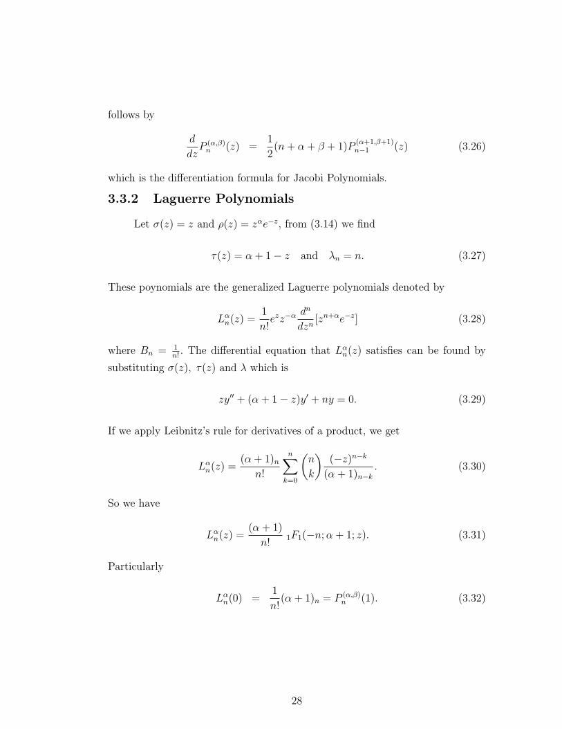
3.3.2 Laguerre Polynomials

Let σ(z) = z and ρ(z) = zαe−z, from (3.14) we find

τ(z) = α + 1− z and λn = n. (3.27)

These poynomials are the generalized Laguerre polynomials denoted by

Lαn(z) =

1

n!ezz−α dn

dzn[zn+αe−z] (3.28)

where Bn = 1n!

. The differential equation that Lαn(z) satisfies can be found by

substituting σ(z), τ(z) and λ which is

zy′′ + (α + 1− z)y′ + ny = 0. (3.29)

If we apply Leibnitz’s rule for derivatives of a product, we get

Lαn(z) =

(α + 1)n

n!

n∑k=0

(n

k

)(−z)n−k

(α + 1)n−k

. (3.30)

So we have

Lαn(z) =

(α + 1)

n!1F1(−n; α + 1; z). (3.31)

Particularly

Lαn(0) =

1

n!(α + 1)n = P (α,β)

n (1). (3.32)

28

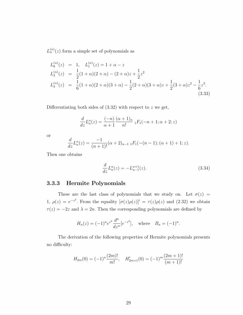
L(α)n (z) form a simple set of polynomials as

L(α)0 (z) = 1, L

(α)1 (z) = 1 + α− z

L(α)2 (z) =

1

2(1 + α)(2 + α)− (2 + α)z +

1

2z2

L(α)3 (z) =

1

6(1 + α)(2 + α)(3 + α)− 1

2(2 + α)(3 + α)z +

1

2(3 + α)z2 − 1

6z3.

(3.33)

Differentiating both sides of (3.32) with respect to z we get,

d

dzLα

n(z) =(−n)

α + 1

(α + 1)n

n!1F1(−n + 1; α + 2; z)

ord

dzLα

n(z) =−1

(n + 1)!(α + 2)n−1 1F1(−(n− 1); (α + 1) + 1; z).

Then one obtains

d

dzLα

n(z) = −Lα+1n−1(z). (3.34)

3.3.3 Hermite Polynomials

These are the last class of polynomials that we study on. Let σ(z) =

1, ρ(z) = e−z2. From the equality [σ(z)ρ(z)]′ = τ(z)ρ(z) and (2.32) we obtain

τ(z) = −2z and λ = 2n. Then the corresponding polynomials are defined by

Hn(z) = (−1)nez2 dn

dzn[e−z2

], where Bn = (−1)n.

The derivation of the following properties of Hermite polynomials presents

no difficulty:

H2m(0) = (−1)n (2m)!

m!, H ′

2m+1(0) = (−1)m (2m + 1)!

(m + 1)!

29

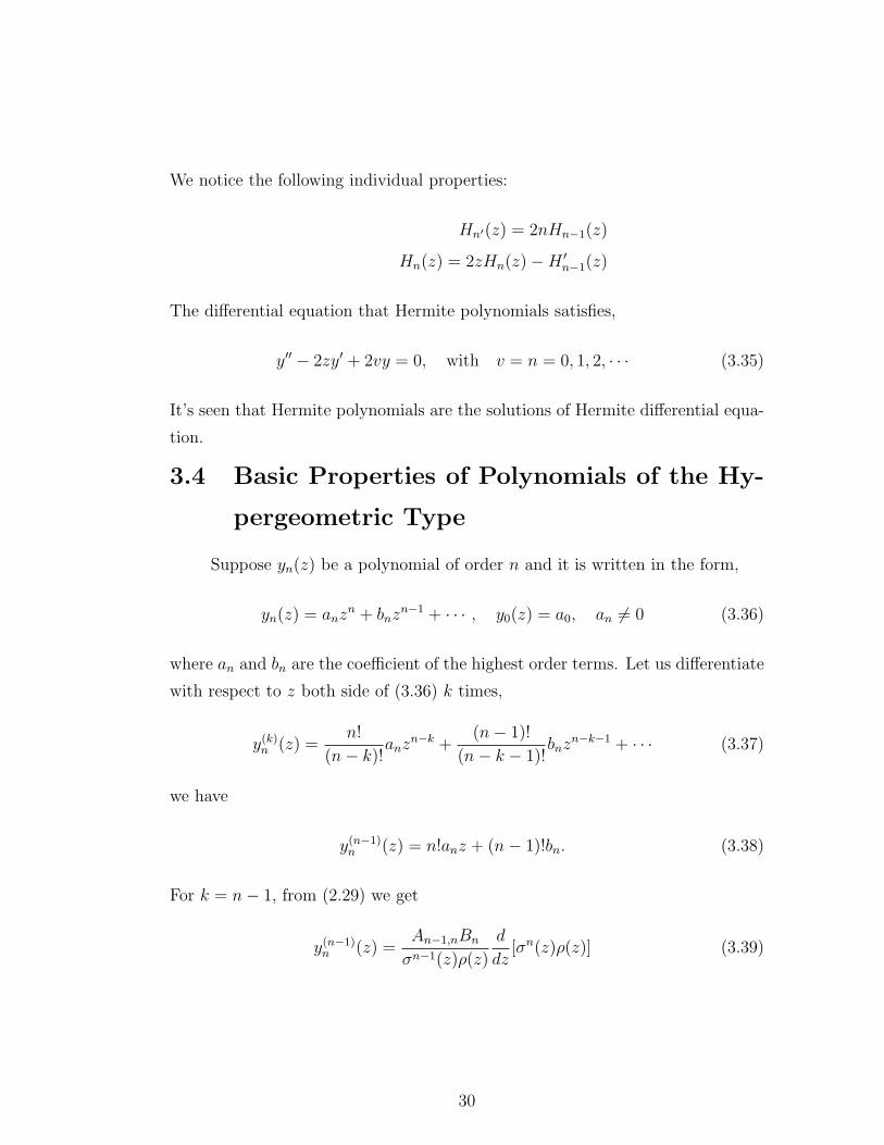
We notice the following individual properties:

Hn′(z) = 2nHn−1(z)

Hn(z) = 2zHn(z)−H ′n−1(z)

The differential equation that Hermite polynomials satisfies,

y′′ − 2zy′ + 2vy = 0, with v = n = 0, 1, 2, · · · (3.35)

It’s seen that Hermite polynomials are the solutions of Hermite differential equa-

tion.

3.4 Basic Properties of Polynomials of the Hy-

pergeometric Type

Suppose yn(z) be a polynomial of order n and it is written in the form,

yn(z) = anzn + bnz

n−1 + · · · , y0(z) = a0, an 6= 0 (3.36)

where an and bn are the coefficient of the highest order terms. Let us differentiate

with respect to z both side of (3.36) k times,

y(k)n (z) =

n!

(n− k)!anz

n−k +(n− 1)!

(n− k − 1)!bnz

n−k−1 + · · · (3.37)

we have

y(n−1)n (z) = n!anz + (n− 1)!bn. (3.38)

For k = n− 1, from (2.29) we get

y(n−1)n (z) =

An−1,nBn

σn−1(z)ρ(z)

d

dz[σn(z)ρ(z)] (3.39)

30

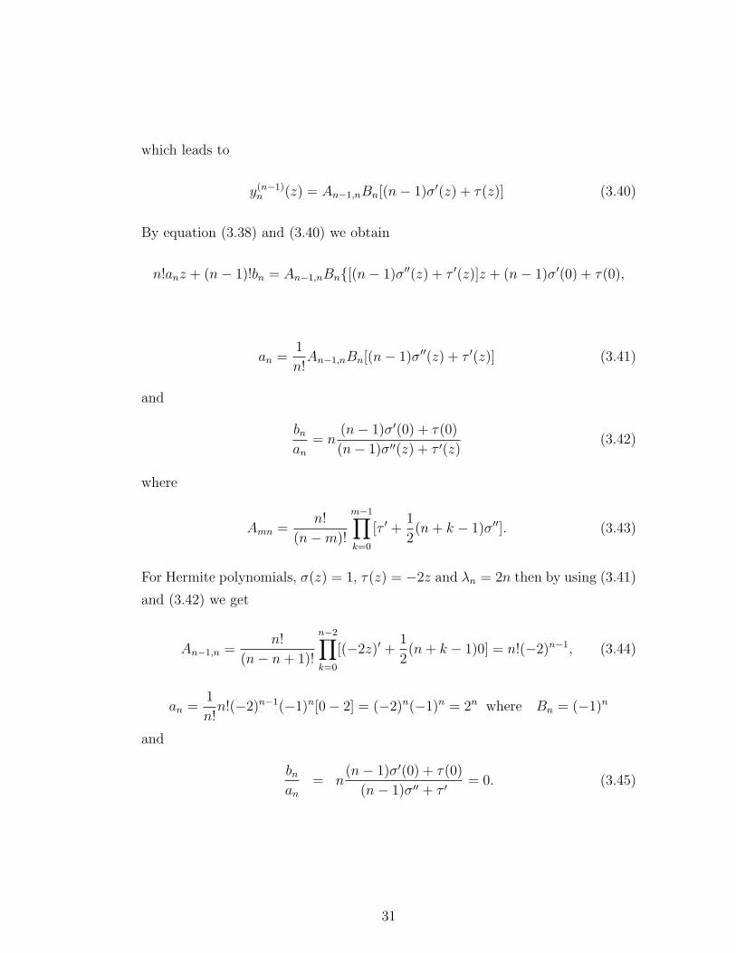
which leads to

y(n−1)n (z) = An−1,nBn[(n− 1)σ′(z) + τ(z)] (3.40)

By equation (3.38) and (3.40) we obtain

n!anz + (n− 1)!bn = An−1,nBn{[(n− 1)σ′′(z) + τ ′(z)]z + (n− 1)σ′(0) + τ(0),

an =1

n!An−1,nBn[(n− 1)σ′′(z) + τ ′(z)] (3.41)

and

bn

an

= n(n− 1)σ′(0) + τ(0)

(n− 1)σ′′(z) + τ ′(z)(3.42)

where

Amn =n!

(n−m)!

m−1∏k=0

[τ ′ +1

2(n + k − 1)σ′′]. (3.43)

For Hermite polynomials, σ(z) = 1, τ(z) = −2z and λn = 2n then by using (3.41)

and (3.42) we get

An−1,n =n!

(n− n + 1)!

n−2∏k=0

[(−2z)′ +1

2(n + k − 1)0] = n!(−2)n−1, (3.44)

an =1

n!n!(−2)n−1(−1)n[0− 2] = (−2)n(−1)n = 2n where Bn = (−1)n

and

bn

an

= n(n− 1)σ′(0) + τ(0)

(n− 1)σ′′ + τ ′= 0. (3.45)

31

For Laguerre polynomial σ(z) = z and τ(z) = α+1− z. Then one obtains

An−1,n =n!

1!

n−2∏k=0

[(α + 1− z)′ +1

2(n + k − 1)0]

= n!n−2∏k=0

(−1) = n!(−1)n−1 (3.46)

and

an =1

n!An−1,nBn[(n− 1)σ′′ + τ ′] =

(−1)n

n!, Bn = 1/n!, (3.47)

bn

an

= n(n− 1)σ′(0) + τ(0)

(n− 1)σ′′ + τ ′= −n(n + α). (3.48)

For Jacobi polynomials if we substitute σ(z) = 1− z2 and τ(z) = β − α −(α + β + 2)z into (3.41) and (3.42) then we obtain

An−1,n = n!n−2∏k=0

[−(α + β + 2) +1

2(n + k − 1)(−2)]

= n!(−1)n−1(α + β + n + 1)n−1 (3.49)

and

an =1

n!An−1,nBn[(n− 1)σ′′ + τ ′] =

1

2nn!(α + β + n + 1)n (3.50)

where Bn = (−1)n

2nn!and

bn

an

= n(n− 1)σ′(0) + τ(0)

(n− 1)σ′′ + τ ′= −n

β − α

α + β + 2n(3.51)

3.4.1 Generating Function

A function Φ(z, t) is called generating function for each polynomial of the

32

hypergeometric type, such that

Φ(z, t) =∞∑

n=0

yn(t)tn

n!, yn(z) = Bnyn(z) (3.52)

where

yn(z) =1

ρ(z)Dn[σn(z)ρ(z)]. (3.53)

It can be shown that the generating function so defined is a function of two

variables whose coefficients of its expansion in powers of t consist of polynomials

of the HG type. Such an expansion is valid at least for sufficiently small |t|.Let us recall the integral form of polynomial solutions

yn(s) =1

ρ(z)

n!

2πi

∫ϕ

σn(s)ρ(s)

(s− z)n+1ds (3.54)

where ϕ is a closed contour surrounding the point at s = z then we can write,

Φ(z, t) =∞∑

n=0

1

ρ(z)

n!

2πi

[∫ϕ

σn(s)ρ(s)

(s− z)n+1ds

]tn

n!. (3.55)

For some z fixed and sufficiently small |t|, we can justify the interchange of

summation and integration which follows that

Φ(z, t) =1

ρ(z)2πi

∫ϕ

ρ(s)

s− z

{ ∞∑n=0

[σ(s)t

s− z]n}

ds

=1

2πiρ(s)

∫ϕ

ρ(s)

s− z − σ(s)tdt (3.56)

since

∞∑n=0

[σ(s)t

s− z]n =

1

1− [σ(s)ts−z

]=

s− z

s− z − σ(s)t. (3.57)

We suppose that there is only one zero of the denominator of the integrand

33

located at s = ξ0(z, t) which is in the near vicinity of s = z and we assume that

such a single pole of the integrand of (3.54) lies inside ϕ so that

Φ(z, t) =1

ρ(z)Resξ0

[ρ(s)

s− z − σ(s)t

](3.58)

where, s− z − σ(s)t

∣∣∣∣s=ξ0

= 0, hence Resξ0f(s) = lims→ξ0(s− ξ0)f(s).

Resξ0

[ρ(s)

s− z − σ(s)t

]= lim

s→ξ0(s− ξ0)

ρ(s)

s− z − σ(s)t

= lims→ξ0

ρ(s) + (s− ξ0)ρ′(s)

1− σ′(s)t=

ρ(s)

1− σ′(s)t

∣∣∣∣s=ξ0(z,t)

which leads to

Φ(z, t) =ρ(s)

ρ(z)

1

1− σ′(s)t

∣∣∣∣s=ξ0(z,t)

(3.59)

for sufficiently small |t|. By the principle of analytic continuation, this is valid

for |t| < R. For a fixed z where R is the distance from the origin to the nearest

singular point of Φ(z, t) with respect to t.

Generating Function for Laguerre Polynomials

If we substitute σ(z) = z and ρ(z) = zαe−z into (3.59) then we have

Φ(z, t) =ρ(s)

ρ(z)

1

1− σ′(s)t

∣∣∣∣s=ξ0

= (s

z)αez−s 1

1− t

∣∣∣∣s=ξ0

(3.60)

ξ0 is the root of s − z − zt, so it can be found ξ0 = z + zt. If we insert ξ0 into

(3.60) then we get

Φ(z, t) = (1 + t)αe−zt(1− t)−1 =∞∑

n=0

Lαn(z) (3.61)

34

which is the generating function for Laguerre Polynomials.

Generating Function for Hermite Polynomials

By substituting σ(z) = 1 and ρ(z) = e−z2into (3.60) we get

Φ(z, t) = ez2−s2

∣∣∣∣s=ξ0(z,t)

=∞∑

n=0

(−1)nHn(z)tn

n!

Here ξ0 is the root of s− z − σ(s)t. So s = ξ0 = z + t. From (3.60) we have

ez2−(z+t)2 =∞∑

n=0

(−1)nHn(z)tn

n!

or

e−2zt−t2 =∞∑

n=0

Hn(z)(−t)n

n!.

Substituting ` = −t we obtain

e−2z`−`2 =∞∑

n=0

Hn(z)sn

n!

and instead of s putting t one obtains

e2zt−t2 =∞∑

n=0

Hn(z)tn

n!. (3.62)

Generating Function for Jacobi Polynomials

Generating function for Jacobi Polynomials can be found by using (3.60)

as

2α+β(1− 2zt + t2)−1(1− t +√

1− 2zt + t2)−α(1 + t +√

1− 2zt + t2)−β

=∞∑

n=0

p(α,β)n (z)tn (3.63)

35

3.4.2 Orthogonality of Polynomial of the Hypergeometric

Type

Let us consider the orthogonality properties of classical polynomials by the

following theorem

Theorem 3.3. Let the coefficients in the differential equation

σ(x)y′′ + τ(x)y′ + λy = 0

be such that

σ(x)ρ(x)xk

∣∣∣∣x=a,b

= 0 for k = 0, 1, · · · (3.64)

at the boundaries of an x-interval (a, b). Then the polynomials of the HG type

which constitute a sequence of real functions of the real argument x

{y0(x), y1(x), · · · , ym(x), · · · , yn(x), · · · } (3.65)

corresponding to different values of λ = λn, i.e.

λ0, λ1, · · · , λm, · · · , λn, · · · (3.66)

are orthogonal on (a, b) in the sense that∫ b

a

ρ(x)ym(x)yn(x)dx = 0 (3.66)

for m 6= n where ρ(x) is now called the weighting function.

Proof. The elements yn and ym of sequence satisfy the differential equations

ym/[σ(x)ρ(x)y′n]′ + λnρ(x)yn = 0 (3.67)

36

yn/[σ(x)ρ(x)y′m]′ + λmρ(x)ym = 0 (3.68)

multiplying the first by yn and second by ym and subtracting we obtain

ym(σρy′n)′ − yn(σρy′m)′ = (λm − λn)ρymyn

which is equal to

d

dx[σρW (ym, yn)] = (λm − λn)ρymyn (3.69)

where W (ym, yn) is the wronskiyen. Integrating both sides from a to b, we get

(λm − λn)

∫ b

a

ρ(x)ym(x)yn(x)dx = σ(x)ρ(x)W (ym, yn)

∣∣∣∣ba

= 0. (3.70)

From the hypothesis the left hand side is equal to zero. Hence, for m 6= n

(λm 6= λn) we must have ∫ b

a

ρ(x)ym(x)yn(x)dx = 0 (3.71)

and more specifically we may write

∫ b

a

ρ(x)ym(x)yn(x)dx = N 2nδmn =

{0 , m 6= n

N 2n , m = n

(3.72)

where Nn is a normalization constant [29].

Orthogonality of Laguerre Polynomials

We know for Laguerre polynomials σ(x) = x and ρ(x) = e−xxα so by using

37

Theorem 3.3 one obtains

σ(x)ρ(x)xk

∣∣∣∣a,b

= e−xxα+1+k

∣∣∣∣x=0,∞

= 0

where (a, b) = (0,∞), then these polynomials are orthogonal provided that α >

−1

Orthogonality of Hermite Polynomials

For Hermite Polynomials σ(x) = 1 and ρ(x) = e−x2, so

σ(x)ρ(x)xk

∣∣∣∣a,b

= e−x2

xk

∣∣∣∣∓∞

= 0

where (a, b) = (−∞, +∞).

Orthogonality of Jacobi Polynomials

For Jacobi Polynomial σ(x) = 1− x2 and ρ(x) = (1 + x)β(1− x)α, then

σ(x)ρ(x)xk

∣∣∣∣a,b

= (1− x)α+1(1 + x)β+1xk

∣∣∣∣x=∓1

= 0

where (a, b) = (−1, 1). So Jacobi polynomials are orthogonal provided that α >

−1 and β > −1.

38

chapter 4

Bessel Polynomials

4.1 Generalized and Reversed Generalized Bessel

Polynomials

We have mentioned in Chapter 2 that the case in which σ(z) has a double

root, i.e. σ(z) = (z − z0)2, can be treated in a different way.

Clearly the differential equation of the HG type

σ(z)y′′ + τ(z)y′ + λy = 0 (4.1)

with σ(z) = (z − z0)2 has polynomial solutions yn(z) of the HG type whenever

λ = λn = −nτ ′(z)− 1

2n(n− 1)σ′′(z) = −n[τ ′(z) + n− 1]. (4.2)

Taking τ ′(z) = a and writing the Taylor polynomial of τ(z) about z = z0, we

have

τ(z) = τ(z0) + a(z − z0) (4.3)

so that the differential equation (4.1) can be written as

y′′ +

[a

z − z0

+τ(z0)

(z − z0)2

]y′ +

λn

(z − z0)2y = 0. (4.4)

If we introduce a new variable s such that

s =1

z − z0

or z − z0 =1

s,

39

ds

dz= −s2,

d2s

dz2= 2s3

dy

dz= −s2dy

ds,

d2y

dz2= s4d2y

ds2+ 2s3dy

ds,

then, the differential equation in (4.4) is transformed to

s2d2y

ds2+ s[2− a− τ(z0)s]

dy

ds+ λny = 0. (4.5)

This is not an equation of the HG type but it is a generalized differential equation.

Therefore, by means of the substitution

y = φ(s)u (4.6)

and the identities

y′

y=

φ′

φ+

u′

u,

y′′

y=

u′′

u+ 2

φ′

φu′ +

φ′′

φ

we transform the last differential equation into the HG type. Actually we obtain,[u′′

u+

2φ′

φ

u′

u+

φ′′

φ

]s2 +

[(φ′

φ+

u′

u)−f(s)

s

]+ λn = 0

leading to

u′′ +

[2φ′

φ− f(s)

s

]u′ +

[φ′′

φ− f(s)

s

φ′

φ+

λn

s2

]u = 0 (4.7)

where f(s) = τ(z0)s + a− 2 is a polynomial in s of degree 1. A suitable form for

φ(s) is s−n. Actually, since

φ(s) = s−n,φ′

φ= −n

s,

φ′′

φ=

n2 + n

s2, n = 0, 1, · · · .

we obtain the differential equation

su′′ − [2n + f(s)]u′ + nτ(z0)u = 0 (4.8)

40

which is an equation of the HG type with

σ(s) = s, τ(s) = −[2n + a− 2 + τ(z0)s], λ = nτ(z0).

This equation has also polynomial solutions because,

λ = λn = −nτ ′ − 1

2n(n− 1)σ′′ = −n[−τ(z0)] + 0 = nτ(z0). (4.9)

The self-adjoint form of (4.8) implies that

[sρ(s)]′ = −[2n + f(s)]ρ(s) = −[2(n− 1) + a + τ(z0)s]ρ(s)

which leads to

ρ(s) = s1−2n−ae−τ(z0)s.

Rodrigues formula defining polynomial solutions, say un(s), of (4.8) is

un(s) = Bnsa+2n−1eτ(z0)s dn

dsn[s1−a−ne−τ(z0)s] (4.10)

where Bn is a constant. In fact these polynomials are closely related to the

Laguerre polynomials Lαn. With t = τ(z0)s, α = 1 − a − 2n, the differential

equation (4.8) takes the form

tu′′(t) + (α + 1− t)u′(t) + nu(t) = 0 (4.11)

which is the Laguerre differential equation. Thus the polynomial solutions are

given by

u(t) = Lαn(t)

so the polynomials in (4.10) are expressible as

un(s) = CnLαn(τ(z0)s) (4.12)

41

in terms of the generalized Laguerre polynomials. It follows then that,

yn(s) =1

snun(s) = s−nLα

n(τ(z0)s)

and

yn(z) = Cn(z − z0)nL1−a−2n

n (τ(z0)

z − z0

) (4.13)

standing for the polynomial solutions of the original equation in (4.1), where Cn

is a constant. It is important to note that we have still polynomials of degree

n even if τ(z0) = 0, in which case the differential equation (4.1) reduces to a

Cauchy-Euler equation. The best known polynomials of the HG type falling into

this catagory, where σ(z) = (z − z0)2 are the generalized Bessel polynomials

denoted by yn(z; a, b). More specifically the generalized Bessel polynomials are

the solutions of the equation

z2y′′ + (b + az)y′ − n(a + n− 1)y = 0. (4.14)

in which z0 = 0 , τ(z0) = b and σ(z) = z2, τ(z) = b+az, λn = −n(a+n−1).

The connection with the Laguerre polynomials is written as

yn(z; a, b) = CnznL1−a−2n

n (b

z), Cn = (

−1

b)nn! (4.15)

and the weighting function ρ(z) satisfies

[z2ρ(z)]′ = (b + az)ρ(z)

from which

ρ(z) = e−b/zza−2 (4.16)

is obtained. Therefore

42

yn(z; a, b) = Bnz2−aeb/zDn[z2n+a−2e−b/z], Bn = (

1

b)n (4.17)

is the Rodrigues formula for the generalized Bessel polynomials [29].

In fact the value of the constant b is not important and a linear transfor-

mation for z transforms (4.15) into

z2y′′ + (2 + az)y′ − n(a + n− 1)y = 0. (4.18)

In this case instead of yn(z; a, b) we can consider a one parameter family of func-

tions denoted by yn(z, a). All formulas above can be reproduced for yn(z, a) if b

is taken 2. Notice that we get polynomial solutions for each n, n = 0, 1, 2, · · ·provided that a is not negative integer or zero.

As a more special case, if a = b = 2 then yn(z, a) reduces to Bessel polyno-

mials yn(z) which satisfy the differential equation

z2y′′ + (2 + 2z)y′ − n(2 + n− 1)y = 0. (4.19)

The Rodrigues formula can be found as

yn(z) := yn(z, 2) = Bne2/zDn[z2ne−2/z], where Bn = (

1

2)n (4.20)

and in terms of the Laguerre polynomials, it can be written as

yn(z) = n!(−z/2)nL−2n−1n (2/z), Cn = (−1/2)nn! (4.21)

Thus normalization is obvious when we introduce the coefficients of the leading

order terms of classical polynomials.

If we replace s by z and set τ(z0) = b in (4.8), (4.10), (4.12) the polynomial

43

solutions un(z) denoted and defined by

θn(z; a) = znyn(z−1; a)

θn(z; a, b) = znyn(z−1; a, b) (4.22)

are called the reverse generalized Bessel polynomials. These polynomials satisfy

the differential equation

zθ′′ − (2n− 2 + a + bz)θ′ + bnθ = 0. (4.23)

The phase reverse can be justified because, if

yn(z; a) = b0zn + b1z

n−1 + · · ·+ bn−1z + bn

then

θn(z; a) = zn[b0(1

z)n + b1(

1

z)n−1 + · · ·+ bn−1(

1

z) + bn]

= b0 + b1z + · · ·+ bn−1zn−1 + bnz

n. (4.24)

Clearly it is seen that reverse generalized Bessel polynomial is a polynomial with

the same coefficients but in reverse order. The differential equation for the gen-

eralized and reverse generalized Bessel polynomials in (6) and (8) respectively

have a basic difference. In (4.17) z = 0 is irregular singular point and z = ∞ is

regular singular point. However in (4.23) the point at the origin z = 0 is a reg-

ular singular point while the point at infinity represents an irregular singularity

which is more preferable. If we use (4.22) we obtain, by routine computations,

the differential equation satisfied by θn = θn(z; a) namely

zθ′′n − (2n− 2 + a + 2z)θn′ + 2nθn = 0. (4.25)

44

For a = b = 2, (4.25) reduces to

zθ′′n − 2(z + n)θn′ + 2nθn = 0. (4.26)

4.2 Recurrence Relation

We shall show that there is a connection between the Bessel function and the

Bessel polynomials. It is well known that the general solution of Bessel differential

equation

z2y′′ + zy′ + (α2z2 − ν2)z = 0 for fixed ν, Reel ν ≥ 0 (4.27)

is given by

y = C1Jν(bz) + C2Yν(bz) (4.28)

where C1 and C2 are arbitrary constants. Jν and Yν denote Bessel functions of

the first and second kinds, respectively. The related differential equation

z2y′′ + zy′ − (z2 + ν2)y = 0, Reel ν ≥ 0 (4.29)

which bears great resemblance to Bessel’s equation, is modified Bessel equation.

It is of the form (4.27) with α2 = −1 . The function Iν(z), Kν(z) are independent

solutions of the modified Bessel equation for all values of ν and its general solution

can be taken to be

y(z) = A1Iν(z) + A2Kν(z). (4.30)

Let y be a solution of (4.29). Under the transformation y = z−νe−zθ, by

substituting y′ and y′′ into (4.29), we obtain

[zθ′′ − (2z + 2ν − 1)θ′ − (2ν − 1)θ]zy = 0. (4.31)

45

As zy(z) 6= 0, it follows that θ(z) satisfies the differential equation

zθ′′ − (2z + 2ν − 1)θ′ + (2ν − 1)θ = 0 (4.32)

which is nothing but the differential equations in (4.26) for reverse Bessel poly-

nomials whenever 2ν − 1 = 2n. This is why the polynomial solutions of (4.14)

and (4.23) are called Bessel polynomials.

By the general theory of linear differential equations, z = 0 is a regular

singular point and in general there exist two independent particular solutions of

the form θ = zα

∞∑m=0

cmzm. By Frobenius’ method one finds that the indicial

equation is,

α(α− 2ν) = 0. (4.33)

The solution of (4.33) are indeed distinct, except for ν = 0. For ν 6= 0, set

θ = θ(z, ν) =∞∑

m=0

cmzm and θ = θ(z, ν) = z2ν∑∞

m=0 c′mzm. After differentiation

and substituting them into (4.32) then we obtain

θ(z, ν) = c0

[1 + z +

(2ν − 1)(2ν − 3)

(2ν − 1)(2ν − 2)

z2

2!+ · · ·+

(2ν − 1)(2ν − 3) · · · (2ν − 2m + 1)

(2ν − 1)(2ν − 2) · · · (2ν −m)

zm

m!+ · · ·

](4.34)

similarly,

θ(z, ν) = c′0z2ν

[1 + z +

(2ν + 1)(2ν + 3)

(2ν + 1)(2ν + 2)

z2

2!+

+ · · ·+ (2ν + 1)(2ν + 3) · · · (2ν + 2m− 1)

(2ν + 1)(2ν + 2) · · · (2ν + m)

zm

m!+ · · ·

]. (4.35)

It is obvious that θ(z, ν) reduces to a polynomial of exact degree n if 2ν =

2n + 1, n = 0, 1, · · · and z−2ν θ(z, ν) reduces to a polynomial of exact degree n if

2ν = −2n − 1, n = 0, 1, · · · In general, it will be sufficient to consider only non

46

negative values for the half integral second parameter so, for ν = n + 12,

θ(z, n +1

2) = c0

[1 + z +

2n(2n− 2)z2

2n(2n− 1)2!+

+ · · ·+ 2n(2n− 2)(2n− 4) · · · (2n− 2(m− 1))

2n(2n− 1)(2n− 2) · · · (2n− (m− 1))

zm

m!

+ · · ·+ 2n(2n− 2)(2n− 4) · · · 4.22n(2n− 1)(2n− 2) · · · (n + 2)(n + 1)

zn

n!

](4.36)

The polynomial defined in (4.36) is the solution of (4.32) while ν = n + 12. The

coefficient of zn in θ(z, n + 12) equals c02n·n!

(2n)!. If we select c0 = (2n)!

2n·n!, the leading

coefficients becomes unity. With this normalization we shall denote θ(z, n + 12)

simply by θn(z). One now easily verifies that

θn(z) =n∑

m=0

an−mzm =n∑

m=0

amzn−m.

In (4.36) if we substitute c0 then we find

an−m =2m−n(2n−m)!

(n−m)!m!, (4.37)

and if we replace m by n−m we get

am =(n + m)!

2m(n−m)!m!, m = 0, 1, 2, · · ·n. (4.38)

The coefficients of generalized Bessel polynomial, yn(z; a, b) could be found by

using the some procedure. The solution of (4.14) is of the form

y = yn(z; a, b) =n∑

k=0

f(n)k zk

where

f(n)k =

n!(n + k + a− 2)(k)

k!(n− k)!bk. (4.39)

47

One verifies that for a = b = 2 [17],

f(n)k =

(n + k)!

k!(n− k)!2k. (4.40)

The corresponding generalization of θn(z; a, b) is obtained most conveniently by

setting

yn(z; a, b) = znθn(z−1; a, b)

The functions Kν(z) and Iν(z) satisfy some recurrence relations [26], [31]

such as

I ′ν(z) +ν

zIν(z) = Iν−1(z), (4.41)

I ′ν(z)− ν

zIν(z) = Iν+1(z), (4.42)

Iν−1(z) + Iν+1(z) = 2I ′ν(z), (4.43)

and

Iν−1(z)− Iν+1(z) =2ν

zIν(z). (4.44)

By the remarkable identity

Kν(z) =π

2

I−ν(z)− Iν(z)

sin νπ, (4.45)

and above recurrence formulas for Iν(z) one obtains

Kν−1(z)−Kν+1(z) = −(2ν/z)Kν(z), (4.46)

48

K ′ν(z) = −Kν−1(z)− (ν/z)Kν(z), (4.47)

Kν−1(z) + Kν+1(z) = −2K ′ν(z), (4.48)

K ′ν(z) = −Kν+1(z) + (ν/z)Kν(z). (4.49)

In general the modified Bessel function of half integral order written as

In+ 12(z) =

1√2πz

[ez

n∑r=0

(−1)r(n + r)!

(n− r)!r!(2z)r+ (−1)n+1e−z

n∑r=0

(n + r)!

(n− r)!r!(2z)r

](4.50)

I−(n+ 12)(z) =

1√2πz

[ez

n∑r=0

(−1)r(n + r)!

(n− r)!r!(2z)r+ (−1)ne−z

n∑r=0

(n + r)!

(n− r)!r!(2z)r

](4.51)

thus, we have

I−(n+ 12) − I(n+ 1

2) =

1√2πz

2(−1)ne−z

n∑r=0

(n + r)!

(n− r)!r!(2z)r. (4.52)

Substituting this identity into (4.45) by taking ν = n + 12, we get

Kn+ 12(z) =

π

2

I(n+1/2) − I−(n+ 12)

sin(n + 12)π

=π

2

2(−1)ne−z∑n

r=0(n+r)!

(n−r)!r!(2z)r

√2πz sin(n + 1

2)π

.

Therefore,

Kn+ 12(z) =

√π

2e−zz−n− 1

2

n∑r=0

(n + r)!

(n− r)!r!2rzn−r. (4.53)

49

We know from (4.38) that

θn(z) =n∑

r=0

(n + r)!

(n− r)!r!2rzn−r.

So we have

Kn+ 12(z) =

√π

2e−zz−n− 1

2 θn(z), (4.54)

and

Kn− 12(z)−Kn+ 3

2(z) = −(2n + 1)

zKn+ 1

2(z). (4.55)

If we insert (4.55) in (4.54) we get

√π/2e−zz−(n−1)−1/2θn−1(z)−

√π/2e−zz−(n+1)−1/2θn+1(z)

= −(2n + 1)

z

√π/2e−zz−n−1/2θn(z), (4.56)

which leads to

zθn−1(z)− 1

zθn+1(z) = −(2n + 1)

zθn(z) (4.57)

or

θn+1(z) = (2n + 1)θn(z) + z2θn−1(z). (4.58)

This is a recurrence relation for θn(z). If we replace in (4.58) z by z−1 and multiply

the result by zn+1,we have

zn+1θn+1(z−1) = (2n + 1)zn+1θn(z−1) + z−2 · zn+1θn−1(z

−1). (4.59)

By using (4.22) we can obtain the following recurrence relation for the BP yn(z)

50

as

yn+1(z) = (2n + 1)zyn(z) + yn−1(z). (4.60)

By starting from θ0(z) = 1 and θ1(z) = 1 + z it can be written, recursively, that

θ2(z) = 3θ1(z) + z2θ0(z) = z2 + 3z + 3,

θ3(z) = 5θ2(z) + z2θ1(z) = z3 + 6z2 + 15z + 15. (4.61)

Similarly, starting from y0(z) = 1 and y1(z) = 1 + z we have

y2(z) = 3zy1(z) + y0(z) = 3z2 + 3z + 1,

y3(z) = 5zy2(z) + y1(z)15z3 + 15z + 6z + 1. (4.62)

Let us differentiate both sides of (4.54) with respect to z. We obtain

K ′n+ 1

2(z) = −

√π

2e−zz−n−1/2θn(z)− (n +

1

2)

√π

2e−zz−n− 3

2 θn(z)

+

√π

2e−zz−n−1/2θ′n(z). (4.63)

In recurrence relation (4.46) if we take v = n + 12

we obtain

K ′n+ 1

2(z) = −Kn− 1

2(z)− (n +

1

2)1

2Kn+ 1

2(z) (4.64)

Using (4.54) and (4.64)

θ′n(z) = θn(z)− zθn−1(z) (4.65)

can be found. If we replace z in (4.65) by z−1 and multiply the result in zn we

have

z2y′n(z) = (nz − 1)yn(z) + yn−1(z). (4.66)

51

So, we found the differentiation formula for yn(z) and θn(z). Similarly by using

(4.46) we have the following recurrence relations:

2zθ′n(z) = (2z + 2n + 1)θn(z)− (z2θn−1(z) + θn+1(z)), (4.67)

2z2y′n(z) = yn−1(z)− (2 + z)yn(z) + yn+1(z), (4.68)

and finally combining (4.65) and (4.67) we get

zθn′(z) = (z + 2n + 1)θn(z)− θn+1(z). (4.69)

Also by using (4.66) and (4.68) we get the corresponding relation

z2y′n−1(z) = yn(z)− (1 + nz)yn−1(z). (4.70)

By the explicit formulas for generalized Bessel polynomials yn(z, a, b) the

first four of these polynomials are therefore given by

y0(z) = 1,

y1(z) = 1 + a(z

b), (4.71)

y2(z) = 1 + 2(a + 1)(z

b) + (a + 1)(a + 2)(

z

b)2,

y3(z) = 1 + 3(a + 2)(z

b) + 3(a + 2)(a + 3)(

z

b)2 +

(a + 2)(a + 3)(a + 4)(z

b)2,

52

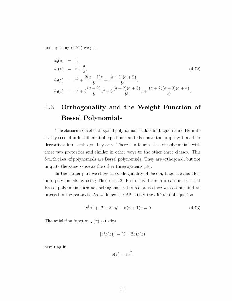
and by using (4.22) we get

θ0(z) = 1,

θ1(z) = z +a

b, (4.72)

θ2(z) = z2 +2(a + 1)z

b+

(a + 1)(a + 2)

b2,

θ3(z) = z3 + 3(a + 2)

bz2 + 3

(a + 2)(a + 3)

b2z +

(a + 2)(a + 3)(a + 4)

b3.

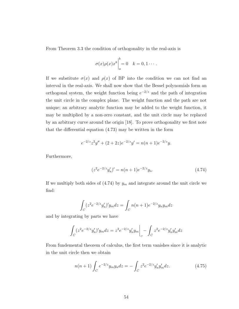
4.3 Orthogonality and the Weight Function of

Bessel Polynomials

The classical sets of orthogonal polynomials of Jacobi, Laguerre and Hermite

satisfy second order differential equations, and also have the property that their

derivatives form orthogonal system. There is a fourth class of polynomials with

these two properties and similar in other ways to the other three classes. This

fourth class of polynomials are Bessel polynomials. They are orthogonal, but not

in quite the same sense as the other three systems [18].

In the earlier part we show the orthogonality of Jacobi, Laguerre and Her-

mite polynomials by using Theorem 3.3. From this theorem it can be seen that

Bessel polynomials are not orthogonal in the real-axis since we can not find an

interval in the real-axis. As we know the BP satisfy the differential equation

z2y′′ + (2 + 2z)y′ − n(n + 1)y = 0. (4.73)

The weighting function ρ(x) satisfies

[z2ρ(z)]′ = (2 + 2z)ρ(z)

resulting in

ρ(z) = e−2z .

53

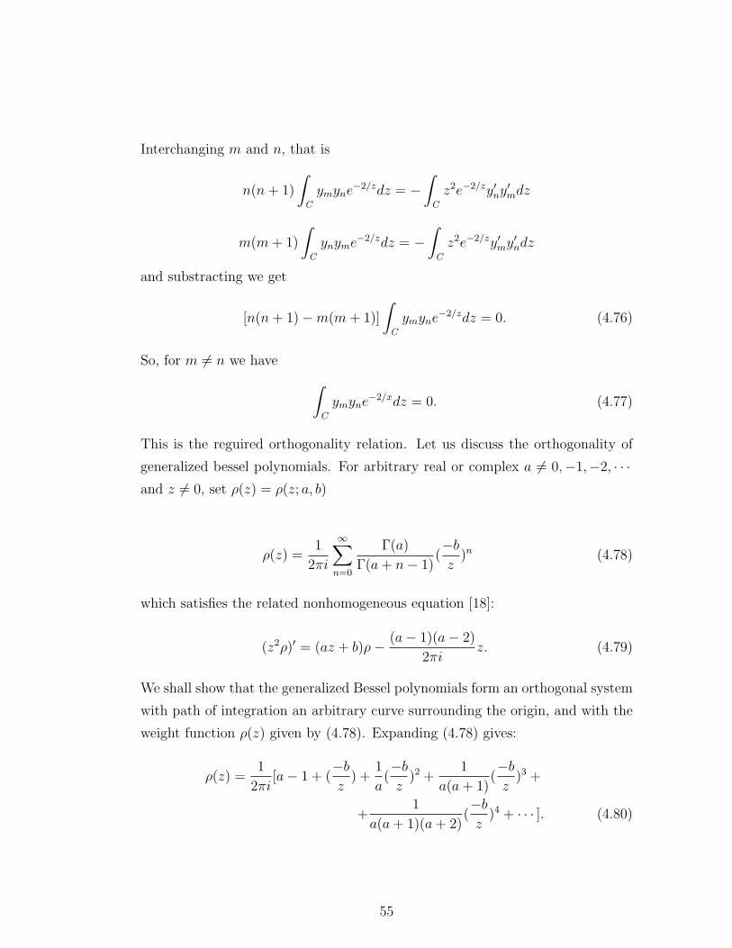
From Theorem 3.3 the condition of orthogonality in the real-axis is

σ(x)ρ(x)xk

∣∣∣∣ba

= 0 k = 0, 1 · · · .

If we substitute σ(x) and ρ(x) of BP into the condition we can not find an

interval in the real-axis. We shall now show that the Bessel polynomials form an

orthogonal system, the weight function being e−2/z and the path of integration

the unit circle in the complex plane. The weight function and the path are not

unique; an arbitrary analytic function may be added to the weight function, it

may be multiplied by a non-zero constant, and the unit circle may be replaced

by an arbitrary curve around the origin [18]. To prove orthogonality we first note

that the differential equation (4.73) may be written in the form

e−2/zz2y′′ + (2 + 2z)e−2/zy′ = n(n + 1)e−2/zy.

Furthermore,

(z2e−2/zy′n)′ = n(n + 1)e−2/zyn. (4.74)

If we multiply both sides of (4.74) by ym and integrate around the unit circle we

find: ∫C

(z2e−2/zy′n)′ymdz =

∫C

n(n + 1)e−2/zynymdz

and by integrating by parts we have∫C

(z2e−2/zy′n)′ymdz = z2e−2/zy′nym

∣∣∣∣C

−∫

C

z2e−2/zy′ny′mdz

From fundemental theorem of calculus, the first term vanishes since it is analytic

in the unit circle then we obtain

n(n + 1)

∫C

e−2/zymyndz = −∫

C

z2e−2/zy′ny′mdz. (4.75)

54

Interchanging m and n, that is

n(n + 1)

∫C

ymyne−2/zdz = −

∫C

z2e−2/zy′ny′mdz

m(m + 1)

∫C

ynyme−2/zdz = −∫

C

z2e−2/zy′my′ndz

and substracting we get

[n(n + 1)−m(m + 1)]

∫C

ymyne−2/zdz = 0. (4.76)

So, for m 6= n we have ∫C

ymyne−2/xdz = 0. (4.77)

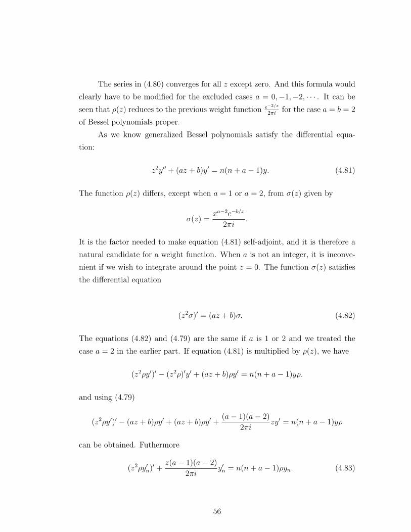
This is the reguired orthogonality relation. Let us discuss the orthogonality of

generalized bessel polynomials. For arbitrary real or complex a 6= 0,−1,−2, · · ·and z 6= 0, set ρ(z) = ρ(z; a, b)

ρ(z) =1

2πi

∞∑n=0

Γ(a)

Γ(a + n− 1)(−b

z)n (4.78)

which satisfies the related nonhomogeneous equation [18]:

(z2ρ)′ = (az + b)ρ− (a− 1)(a− 2)

2πiz. (4.79)

We shall show that the generalized Bessel polynomials form an orthogonal system

with path of integration an arbitrary curve surrounding the origin, and with the

weight function ρ(z) given by (4.78). Expanding (4.78) gives:

ρ(z) =1

2πi[a− 1 + (

−b

z) +

1

a(−b

z)2 +

1

a(a + 1)(−b

z)3 +

+1

a(a + 1)(a + 2)(−b

z)4 + · · · ]. (4.80)

55

The series in (4.80) converges for all z except zero. And this formula would

clearly have to be modified for the excluded cases a = 0,−1,−2, · · · . It can be

seen that ρ(z) reduces to the previous weight function e−2/z

2πifor the case a = b = 2

of Bessel polynomials proper.

As we know generalized Bessel polynomials satisfy the differential equa-

tion:

z2y′′ + (az + b)y′ = n(n + a− 1)y. (4.81)

The function ρ(z) differs, except when a = 1 or a = 2, from σ(z) given by

σ(z) =xa−2e−b/x

2πi.

It is the factor needed to make equation (4.81) self-adjoint, and it is therefore a

natural candidate for a weight function. When a is not an integer, it is inconve-

nient if we wish to integrate around the point z = 0. The function σ(z) satisfies

the differential equation

(z2σ)′ = (az + b)σ. (4.82)

The equations (4.82) and (4.79) are the same if a is 1 or 2 and we treated the

case a = 2 in the earlier part. If equation (4.81) is multiplied by ρ(z), we have

(z2ρy′)′ − (z2ρ)′y′ + (az + b)ρy′ = n(n + a− 1)yρ.

and using (4.79)

(z2ρy′)′ − (az + b)ρy′ + (az + b)ρy′ +(a− 1)(a− 2)

2πizy′ = n(n + a− 1)yρ

can be obtained. Futhermore

(z2ρy′n)′ +z(a− 1)(a− 2)

2πiy′n = n(n + a− 1)ρyn. (4.83)

56

If we multiply equation (4.83) by yk and integrate around the unit circle we get

∫C

(z2ρy′n)′ykdz +

∫C

z(a− 1)(a− 2)

2πiy′nykdz = n(n + a− 1)

∫C

ρynykdz. (4.84)

By integrating by parts we have

z2ρy′nyk

∣∣∣∣C

−∫

C

z2ρy′ny′kdz +

∫C

z(a− 1)(a− 2)

2πiy′nykdz = n(n + a− 1)

∫C

ρynykdz.

From Cauchy’s Theorem, one obtains∫C

z(a− 1)(a− 2)

2πiy′nykdz = 0

and z2ρy′nyk is analytic so by the fundemental theorem it vanishes. Then (4.84)

becomes

n(n + a− 1)

∫C

ρynykdz = −∫

C

z2ρy′ny′kdz. (4.85)

Interchanging n and k , that is

n(n + a− 1)

∫C

ynykρdz = −∫

C

z2ρy′ny′kdz

k(k + a− 1)

∫C

ykynρdz = −∫

C

z2ρy′ky′ndz

and substracting gives:

[n(n + a− 1)− k(k + a− 1)]

∫C

ykynρdz = 0. (4.86)

Finally, for n 6= k we have ∫C

ykynρdz = 0,

which shows that the polynomials are orthogonal with weight function ρ(z). As

we show before, in real-axis Bessel polynomials are not orthogonal and also gen-

eralized Bessel polynomials are not orthogonal in the real-axis with the function

57

ρ(z) = e−b/zza−2 because we can not find an interval that satisfies condition which

is given in Theorem 3.3. Let us calculate for n = k ,the value of∫C

yn(z; a, b)2ρ(z; a, b)dz

and ∫C

zkyn(z; a, b)ρ(z; a, b)dz.

Suppose pn(z) =n∑

m=0

cmzm be an arbitrary polynomial of degree n. The weight

function ρ is defined by

ρ(z; a, b) =1

2πi

∞∑r=0

Γ(a)

Γ(a + r − 1)(−b

z)r.

So, ∫|z|=1

zkpn(z)ρ(z)dz =1

2πi

∫|z|=1

zkpn(z)(∞∑

r=0

Γ(a)

Γ(a + r − 1)(−b

z)r)dz.

We may interchange summation and integration since∑∞

r=0Γ(a)

Γ(a+r−1)(−b

z)r con-

verges. ∫|z|=1

zkpn(z)ρ(z)dz =1

2πi

∞∑r=0

(−1)rbrΓ(a)

Γ(a + r − 1)

n∑m=0

∫|z|=1

cmzk+m−rdz

Using Cauchy’s Integral Formula and Cauchy’s Teorem we obtain,∫|z|=1

zk+m−rdz = 0, for k + m− r 6= −1

and ∫|z|=1

zk+m−rdz = 2πi for k + m− r = −1.

58

Therefore, ∫|z|=1

zkpn(z)ρ(z)dz =∑

k+m−r=−1

cmΓ(a)

Γ(a + r − 1(−1)rbr

=n+k+1∑r=k+1

(−1)rbrcr−k−1Γ(a)

Γ(a + r − 1).

We are interested in the case when pn(z) = yn(z; a, b) =n∑

m=0

f (n)m zm. From (4.39)

we have

f (n)m =

(n

m

)b−m(n + m + a− 2)(n + m + a− 3) · · · (n + a− 1),

so that the sum may be written as [17], [24]

∫|z|=1

zkyn(z; a, b)ρ(z; a, b)dz =n+k+1∑r=k+1

(−1)rbr

(n

r − k − 1

)(n + r − k − 1 + a− 2)

(n + r − k − 1 + a− 3) · · · (n + a− 1)b−(r−k−1) Γ(a)

Γ(a + r − 1)

=n+k+1∑r=k+1

(−1)rbr n!(n + r − k + a− 3) · · · (n + a− 1) · (a− 1)!

(r − k − 1)!(n− r + k + 1)!(a + r − 2) · · · (a + 1)a(a− 1)!

=n∑

v=r−k−1=0

(−1)k+1bk+1(−1)v n!(n + v + a− 2) · · · (n + a− 1)

v!(n− v)!(k + v + a− 1) · · · (a + 1)a.

This leads to

∫|z|=1

zkyn(z; a, b)ρ(z; a, b)dz =(−b)k+1

(k + n + a− 1) · · · (a + 1)(a)

n∑v=0

(−1)v

(n

v

)(n + v + a− 2) · · · (n + a− 1)(k + v + a) · · · (k + n + a− 1)(4.87)

59

Lemma 4.1.n∑

v=0

(n

v

)(k − n

t− v

)=

(k

t

)Proof.

k∑t=0

(k

t

)xt = (x + 1)k = (x + 1)n(x + 1)k−n

=n∑

v=0

(n

v

)xv

k−n∑w=0

(k − n

w

)xw

=n∑

v=0

(n

v

) k−n∑w=0

(k − n

w

)xw+v

By changing v + w = t,

k∑t=0

(k

t

)xt =

k∑t=0

xt

n∑v=0

(n

v

)(k − n

t− v

)[17] (4.88)

Lemma 4.2. The function

f(x) =n∑

v=0

(−1)v

(n

v

)Γ(k + n + x + 1)

Γ(n + x)(k + v + x)(k − 1 + v + x) · · · (n + v + x)(4.89)

is independent of x, and has the value k(k − 1) · · · (k − n + 1); in particular, for

k < n one has f(x) = 0.

Proof. For k ≥ n (4.89) is equivalent to

f(x) =n∑

v=0

(−1)v

(n

v

)(k + n + x) · · · (k + v + x) · · · (n + v + x) · · · (n + x)

(k + v + x) · · · (n + v + x)

(4.90)

Clearly f(x) is a rational function and could have poles at most for x = −m,

n ≤ m ≤ k + n. In fact, as seen from (4.90), all these poles cancel and f(x) is

60

a polynomial of degree at most n. We shall show that limx→−m

f(x) exists for all

these k + 1 values of m in the given range and that all these limits equal k!(k−n)!

,

independently of m. It then follows that the polynomial f(x) of degree n < k +1

equals k!(k−n)!

identically, as claimed.

To find the limit, set m = n + t, 0 ≤ t ≤ n, t ∈ Z, x = −n − s. Then by

(4.90)

lims→t

f(−n−s) = lims→t

Γ(k − s + 1)

(t− s)(t− 1− s)(−s)Γ(−s)

n∑v=0

(−1)v

(n

v

)(t− s) · · · (−s)

(k + v − n− s) · · · (v − s)

= lims→t

Γ(k − s + 1)

Γ(t− s)

n∑v=0

(−1)v

(n

v

)(t− s) · · · (−s)Γ(−s)

(k + v − n− s) · · · (v − s)Γ(−s)

= Γ(k − 1 + 1) lims→t

n∑v=0

(−1)v

(n

v

)(t− s) · · · (−s)Γ(−s)

(k + v − n− s) · · · (v − s)r(−s)

because for t < v ≤ n, −s < t − s < v − s and the vanishing factor of the

numerator not cancelled by a corresponding factor of the denominator. It follows

that therefore

lims→t

f(−n− s) = Γ(k − t + 1) lims→t

t∑v=0

(−1)v

(n

v

)Γ(t− s)(v − s− 1) · · · (−s)

Γ(k + v − n− s)

= Γ(k − t + 1)t∑

v=0

(−1)v

(n

v

)(v − t− 1) · · · (1− t)(−t)

Γ(k + v − n− t)

= (k − t)!t∑

v=0

(n

v

)t!

(t− v)!(k + v − n− t)!

=(k − t)!t!

(k − n)!

t∑v=0

(n

v

)(k − n

t− v

).

By Lemma 4.1 the last sum equals to(

kt

), so that

limx→−m

f(x) =(k − t)!t!

(k − n)!

k!

t!(k − t)!=

k!

(k − n)!.

61

as claimed. The lemma is proved [17].

Using Lemma 4.2, let us calculate the sum in (4.87): The sum becomes

n∑v=0

(−1)v

(n

v

)(n + v + x− 1) · · · (n + x− 1)(n + x)(k + v + x− 1) · · · (k + n + x)

=n∑

v=0

(−1)v

(n

v

)(k + n + x)(k + n + x− 1) · · · (k + v + x) · · · (n + v + x) · · · (n + x)

(k + v + x) · · · (n + v + x)

=∑v=0

n(−1)v

(n

v

)Γ(k + n + x + 1)

Γ(n + x)

1

(k + v + x)(k + v + x− 1) · · · (n + v + x)

where x = a− 1. This leads to

k(k − 1) · · · (k − n + 1) =k!

(k − n)!

by Lemma 4.2. If we inset this value in (4.87) we obtain∫|z|=1

zkyn(z; a, b)ρ(z; a, b)dz =(−b)k+1

(k + n + a− 1) · · · (a + 1)a

k!

(k − n)!

=(−b)k+1Γ(k + 1)Γ(a)

Γ(k + n + a)Γ(k + 1− n). (4.91)

As a consequences of from Lemma 4.2 we have for 0 ≤ k < n,

∫|z|=1

zkyn(z; a, b)ρn(z; a, b)dz = 0. (4.92)

If a > 0 ∫|z|=1

zkyn(z; a, b)ρ(z; a, b)dz = (−b)k+1 (a− 1)!k!

(k + n + a− 1)!(k − n)!

For a = 2,

ρ(z; 2, b) =∞∑

n=0

(−1)n(b/z)n

n!= e−b/z.

62

Thus when a = 2 and k ≥ n,

∫|z|=1

zkyn(z; 2, b)ρ(z; 2, b)dz = (−b)k+1 k!

(k + n + 1)!(k − n)!. (4.93)

For a = b = 2 and k ≥ n, we obtain

∫|z|=1

zkyn(z; 2, 2)ρ(z; 2, 2)dz =(−2)k+1k!

(k + n + 1)!(k − n)!(4.94)

For n = k (4.94) can be written as∫|z|=1

y2n(z; a, b)ρ(z; a, b)dz =

∫|z|=1

f (n)n znyn(z; a, b)ρ(z; a, b)dz

= f (n)n

∫|z|=1

znyn(z; a, b)ρ(z; a, b)dz

From (4.37) we have

f (n)n = b−n(2n + a− 2)(2n + a− 3) · · · (n + a− 1) = b−n Γ(2n + a− 1)

Γ(n + a− 1).

So by substituting f(n)n it follows that

f (n)n

∫|z|=1

znyn(z; a, b)ρ(z; a, b)dz = f (n)n (−b)n+1 Γ(n + 1)Γ(a)

Γ(2n + a)

=b−nΓ(2n + a− 1)Γ(a)Γ(n + 1)(−b)n+1

Γ(2n + a)Γ(n + a− 1)

=(−1)n+1bn!Γ(a)

(2n + a− 1)Γ(n + a− 1). (4.96)

In particular, if a = b = 2, then∫|z|=1

y2n(z; 2, 2)e−2/zdz = (−1)n+1 2

2n + 1. (4.97)

63

By using yn(z) = znθn(z−1; a, b) and setting

ρ1(z; a, b) =z2

2πi

∞∑r=0

Γ(a)

Γ(a + r − 1)(−bz)r (4.98)

we obtain, for k ≥ n, that∫|z|=1

z−k(z−nθn(z; a, b))ρ1(z; a, b)dz =(−1)k+1bk+1Γ(a)Γ(k + 1)

Γ(k + a + n)Γ(k + 1− n). (4.99)

It follows that for k = n,∫|z|=1

(z−nθn(z; a, b))2ρ1(z; a, b)dz = (−1)n+1 bn!

2n + a− 1

Γ(a)

Γ(n + a− 1)(4.100)

4.4 Relations of the Bessel Polynomials to the

Classical Orthogonal Polynomials and to Other

functions

4.4.1 Relations to Hypergeometric Functions

In Chapter 2 we give the definition of generalized hypergeometric series as

AFB(α1, α2, · · ·αA; γ1, γ2, · · · , γB; z) =∞∑

n=0

(α1)n(α2)n · · · (αA)n

(γ1)n(γ2)n · · · (γB)n

zn

n!. (4.101)

For A = 2 and B = 0, (4.101) gives

2F0(α1, α2; z) =∞∑

n=0

(α1)n(α2)nzn

n!.

Let us take α1 = −n, α2 = n + a− 1 and z → −zb

in 2F0(α1, α2, z), where n is a

natural number so 2F0(−n, n + a− 1; −zb

) is

64

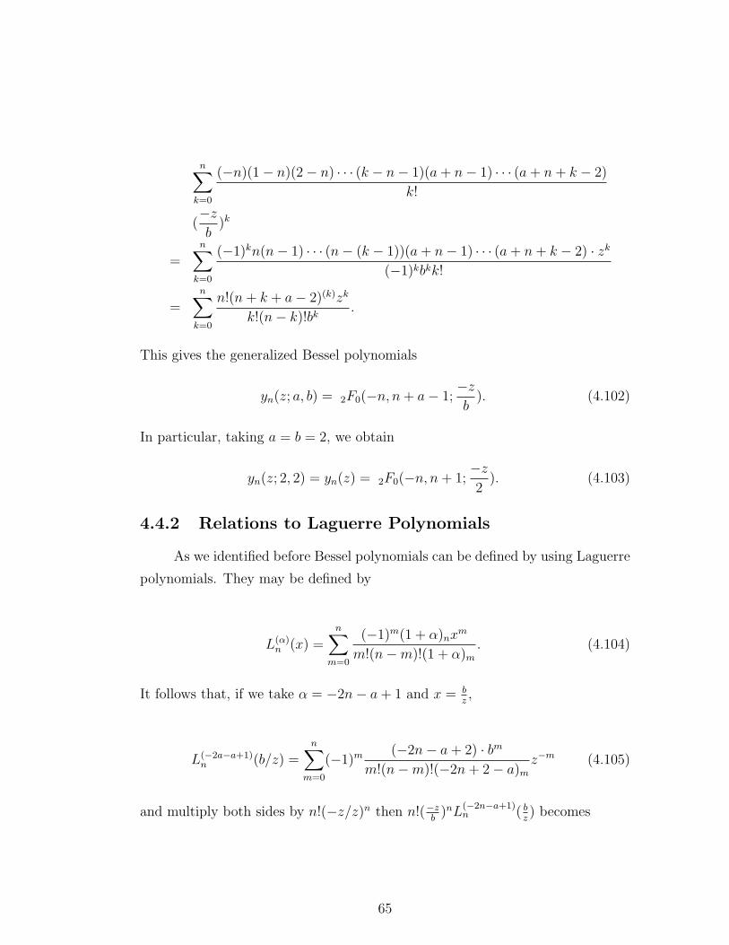
n∑k=0

(−n)(1− n)(2− n) · · · (k − n− 1)(a + n− 1) · · · (a + n + k − 2)

k!

(−z

b)k

=n∑

k=0

(−1)kn(n− 1) · · · (n− (k − 1))(a + n− 1) · · · (a + n + k − 2) · zk

(−1)kbkk!

=n∑

k=0

n!(n + k + a− 2)(k)zk

k!(n− k)!bk.

This gives the generalized Bessel polynomials

yn(z; a, b) = 2F0(−n, n + a− 1;−z

b). (4.102)

In particular, taking a = b = 2, we obtain

yn(z; 2, 2) = yn(z) = 2F0(−n, n + 1;−z

2). (4.103)

4.4.2 Relations to Laguerre Polynomials

As we identified before Bessel polynomials can be defined by using Laguerre

polynomials. They may be defined by

L(α)n (x) =

n∑m=0

(−1)m(1 + α)nxm

m!(n−m)!(1 + α)m

. (4.104)

It follows that, if we take α = −2n− a + 1 and x = bz,

L(−2a−a+1)n (b/z) =

n∑m=0

(−1)m (−2n− a + 2) · bm

m!(n−m)!(−2n + 2− a)m

z−m (4.105)

and multiply both sides by n!(−z/z)n then n!(−zb

)nL(−2n−a+1)n ( b

z) becomes

65

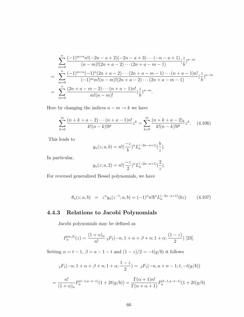
n∑m=0

(−1)m+nn!(−2n− a + 2)(−2n− a + 3) · · · (−n− a + 1)

(n−m)!(2n + a− 2) · · · (2n + a−m− 1)(z

b)n−m

=n∑

m=0

(−1)m+n(−1)n(2n + a− 2) · · · (2n + a−m− 1) · · · (n + a− 1)n!

(−1)mm!(n−m)!(2n + a− 2) · · · (2n + a−m− 1)(z

b)n−m

=n∑

m=0

(2n + a−m− 2) · · · (n + a− 1)n!

m!(n−m)!(z

b)n−m.

Here by changing the indices n−m → k we have

m∑k=0

(n + k + a− 2) · · · (n + a− 1)n!

k!(n− k)!bkzk =

m∑k=0

(n + k + a− 2)k

k!(n− k)!bkzk. (4.106)

This leads to

yn(z; a, b) = n!(−z

b)nL(−2n−a+1)

n (b

z).

In particular,

yn(z; a, 2) = n!(−z

2)nL(−2n−a+1)

n (2

z).

For reversed generalized Bessel polynomials, we have

θn(z; a, b) = znyn(z−1; a, b) = (−1)nn!bnL(−2n−a+1)n (bz) (4.107)

4.4.3 Relations to Jacobi Polynomials

Jacobi polynomials may be defined as

P (α,β)n (z) =

(1 + α)n

n!2F1(−n, 1 + α + β + n; 1 + α;

(1− z)

2) [23].

Setting α = t− 1, β = a− 1− t and (1− z)/2 = −t(y/b) it follows

2F1(−n, 1 + α + β + n; 1 + α;1− z

2) = 2F1(−n, a + n− 1; t;−t(y/b))

=n!

(1 + α)n

P (t−1,a−t−1)n (1 + 2t(y/b)) =

Γ(α + 1)n!

Γ(n + α + 1)P (t−1,a−t−1)

n (1 + 2t(y/b)

66

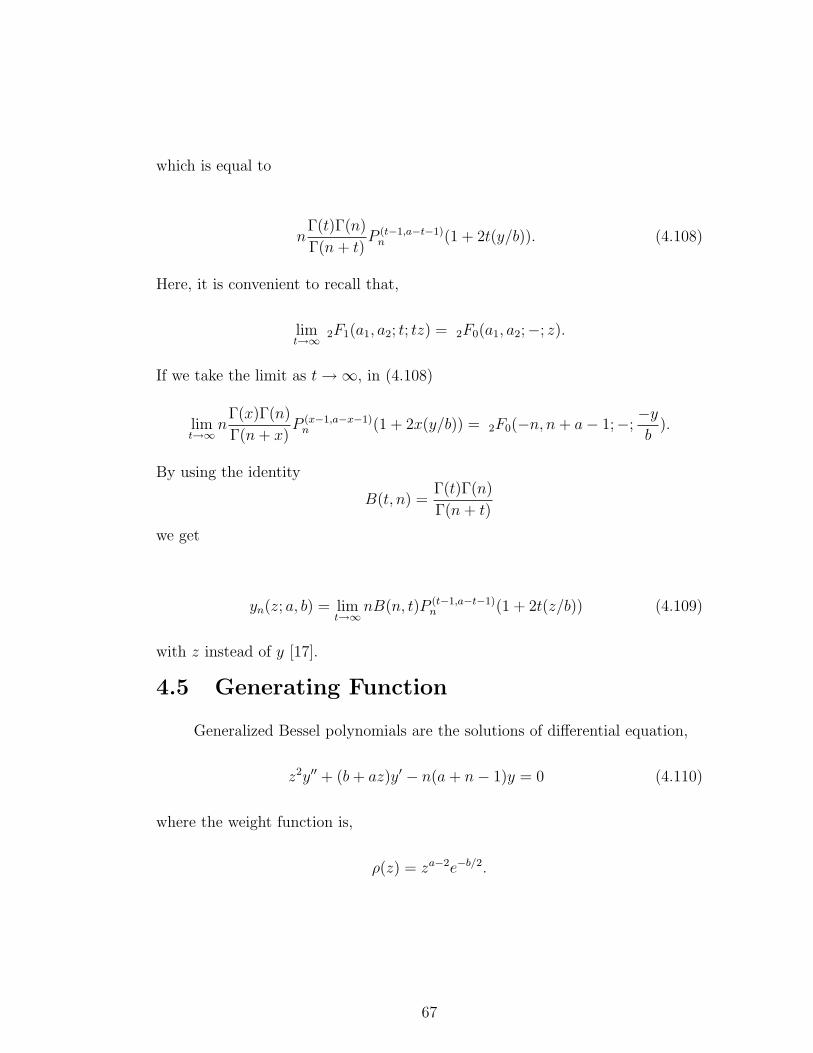
which is equal to

nΓ(t)Γ(n)

Γ(n + t)P (t−1,a−t−1)

n (1 + 2t(y/b)). (4.108)

Here, it is convenient to recall that,

limt→∞ 2F1(a1, a2; t; tz) = 2F0(a1, a2;−; z).

If we take the limit as t →∞, in (4.108)

limt→∞

nΓ(x)Γ(n)

Γ(n + x)P (x−1,a−x−1)

n (1 + 2x(y/b)) = 2F0(−n, n + a− 1;−;−y

b).

By using the identity

B(t, n) =Γ(t)Γ(n)

Γ(n + t)

we get

yn(z; a, b) = limt→∞

nB(n, t)P (t−1,a−t−1)n (1 + 2t(z/b)) (4.109)

with z instead of y [17].

4.5 Generating Function

Generalized Bessel polynomials are the solutions of differential equation,

z2y′′ + (b + az)y′ − n(a + n− 1)y = 0 (4.110)

where the weight function is,

ρ(z) = za−2e−b/2.

67

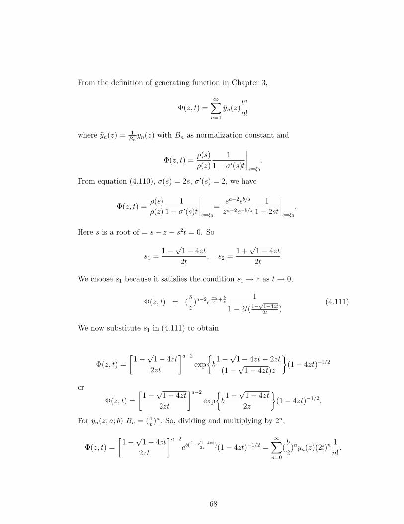
From the definition of generating function in Chapter 3,

Φ(z, t) =∞∑

n=0

yn(z)tn

n!

where yn(z) = 1Bn

yn(z) with Bn as normalization constant and

Φ(z, t) =ρ(s)

ρ(z)

1

1− σ′(s)t

∣∣∣∣s=ξ0

.

From equation (4.110), σ(s) = 2s, σ′(s) = 2, we have

Φ(z, t) =ρ(s)

ρ(z)

1

1− σ′(s)t

∣∣∣∣s=ξ0

=sa−2eb/s

za−2e−b/z

1

1− 2st

∣∣∣∣s=ξ0

.

Here s is a root of = s− z − s2t = 0. So

s1 =1−

√1− 4zt

2t, s2 =

1 +√

1− 4zt

2t.

We choose s1 because it satisfies the condition s1 → z as t → 0,

Φ(z, t) = (s

z)a−2e

−bs

+ bz

1

1− 2t(1−√

1−4zt2t

)(4.111)

We now substitute s1 in (4.111) to obtain

Φ(z, t) =

[1−

√1− 4zt

2zt

]a−2

exp

{b1−

√1− 4zt− 2zt

(1−√

1− 4zt)z

}(1− 4zt)−1/2

or

Φ(z, t) =

[1−

√1− 4zt

2zt

]a−2

exp

{b1−

√1− 4zt

2z

}(1− 4zt)−1/2.

For yn(z; a; b) Bn = (1b)n. So, dividing and multiplying by 2n,

Φ(z, t) =

[1−

√1− 4zt

2zt

]a−2

eb( 1−√

1−4zt2z

)(1− 4zt)−1/2 =∞∑

n=0

(b

2)nyn(z)(2t)n 1

n!.

68

and replacing 2t by s[1−

√1− 2zs

zs

]a−2

eb( 1−√

1−2zs2z

)(1− 2zs)−1/2 =∞∑

n=0

(b

2)nyn(z)sn 1

n!.

Futhermore,[(1−

√1− 2zs)(1 +

√1− 2zs)

zs(1 +√

1− 2zs)

]a−2

eb2z

(1−√

1−2zs)(1− 2zs)−1/2

=∞∑

n=0

(b

2)nyn(z)sn 1

n!.

and replacing s by t, we obtain the generating function for yn(z; a, b) as

Φ(z, t) = (1− 2zt)−1/2

[1 +

√1− 2zt

2

]2−a

exp

{(

b

2z)(1−

√1− 2zt)

}=

∞∑n=0

(b

2)ntnyn(z; a, b)

1

n!. (4.112)

For b = 2 generating function for yn(z; a, 2) is

(1− 2tz)−1/2

[1 +

√1− 2zt

2]2−a exp

{1

z(1−

√1− 2zt)

}=

∞∑n=0

yn(z; a)tn

n!.

In particular, if a = b = 2, we have the generating function for Bessel polynomials

as

(1− 2zt)−1/2 exp

{1

z(1−

√1− 2tz)1/2

}=

∞∑n=0

yn(z)

n!tn.

If we replace yn(z; a, b) by znθn(z−1; a, b) in (4.111) we get

(1− 2zt)−1/2

[1 +

√1− 2zt

2

]2−a

exp

{b

2z1−

√1− 2zt

}=

∞∑n=0

(b

2)nznθn(z−1; a, b)

tn

n!.

69

We now replace z by z−1 to get

(z

z − 2t)1/2

[1 + ( z

z−2t)−1/2

2

]2−a

exp

{bz

2(1− (

z

z − 2t)−1/2

}=

∞∑n=0

(b

2)nθn(z; a, b.) (4.113)

If we insert b = 2 in (4.113) we have

(z

z − 2t)1/2

[1 + ( z

z−2t)−1/2

2

]2−a

exp

{z(1− (

z

z − 2t)−1/2

}=

∞∑n=0

θn(z; a)(t

z)n.

Particularly, for a = b = 2 one obtains

(z

z − 2t)1/2 exp

{z(1− (

z

z − 2t)−1/2

}=

∞∑n=0

θn(z)(t

z)n.

70

references

[1] M. Abramowitz and I.A. Stegun, Handbook of Mathematical Functions,

Dover Publication, New York (1970).

[2] G. Andrews, R. Askey, R. Roy, Special Functions, Cambridge University

Press, New York (1999).

[3] L. C. Andrews, Special Functions of Mathematics for Engineers, McGraw-

Hill, New York (1992).

[4] R. P. Agorwal, On the Bessel Polynomials, Canad. J. Math., 6, 410 (1954).

[5] W. A. Al-Salam, The Bessel Polynomials, Duke Math. J., 24, 529 (1957).

[6] C. W. Barnes, Remarks on the Bessel Polynomials, Amer. Math. Monthly,

80, 1034 (1973).

[7] W. W. Bell, Special Functions for Scientists and Engineers, D. Van Nostrond

Company, London (1968).

[8] F. Bowman, Introduction to Bessel Functions, Dover Publication, New York

(1958).

[9] R. A. Brualdi, Remarks on the Zeros of Bessel Polynomials, Amer. Math.

Monthly, 83, 122 (1976).

[10] H. Buchholz, The Confluent Hypergeometric Function, Springer-Verlag,

Berlin (1969).

[11] J. L. Burchnall, The Bessel Polynomials, Canad. J. Math., 3, 62 (1951).

[12] B. C. Carlson, Special Functions of Applied Mathematics, Academic Press,

London (1977).

[13] M. Chen, C. Feng, H. Srivastova, Some Generating Functions for the Gen-

eralized Bessel Polynomials, 87, 351 (1992).

71

[14] M. Chen, A Note on Certain Generating Functions for the Generalized Bessel

Polynomials,180, 151 (1993).

[15] T. M. Dunster, Uniform Asymptotic Exponsions for the Reverse Generalized

Bessel Polynomials and Related Functions, SIAM J. Math. Anal., 32, 987

(2001).

[16] A. Gray, G. B. Mathews, A Trease on Bessel Functions and Their Applica-

tions to Physic, Dover Publication, New York (1966).

[17] E. Grosswald, Bessel Polynomials, Lecture Notes in Mathematics, 698,

Springer-Verlag, New York (1978).

[18] H. L. Krall, Orrin Frink, A New Class of Orthogonal Polynomials: The Bessel

Polynomials, Trans. Amer Math. Soc., 65, 100 (1949).

[19] K. H. Kwon, L. Little John, B. Yoo New Characterizations of Classical Or-

thogonal Polynomials, Indag. Math. N.S, 7 (2), 199 (1996).

[20] L. Luke, The Special Functions and Their Approxinations, Vol.1, Academic

Press, New York (1969).

[21] N. W. McLachlan, Bessel Functions for Engineers, Oxford University Press,

London (1955).

[22] M. Nassif, Note on the Bessel Polynomials, Trans. Amer. Math. Soc., 77,

408 (1954).

[23] F. J.M. Olver, Asymptotics and Special Functions, Academic Press, New

York (1974).

[24] M. A. Ozarslan, Bessel Polinomları, Yuksek Lisans Tezi, Ankara Universitesi

Fen Bilimleri Enstitusu, (2000).

[25] E. Rainville, Special functions, The Macmillon Company, New York (1965).

[26] F. Relton, Applied Bessel Functions, Dover, New York (1965).

72

[27] L. Slater, Generalized Hypergeometric Functions, Cambridge at the Uni.

Press, Cambridge (1966).

[28] G. Szego, Orthogonal Polynomials, Amer. Mat. Soci. Coll. Publi., Vol. 23,

Phode Island (1975).

[29] H. Taseli, Lecture Notes in Special Functions, METU, Department in Math-

ematics (2003).

[30] S. Yang, Some Families of Generating Functions for the Bessel Polynomials,

Jour. of Math. Analy. and App. 211, 314 (1997).

[31] G. N. Watson, A trease on the theory of Bessel Functions, Cambridge Uni.

Press, Cambridge (1946).

[32] R. Wong, J. M. Zhong, Asympotic Expansions of the Generalized Bessel

Polynomials, Jour. of Comp. and App. Math. 85, 87 (1997).

73