Generalized Chebyshev polynomials and plane trees

Anton BankevichSt. Petersburg State University

Jass’07

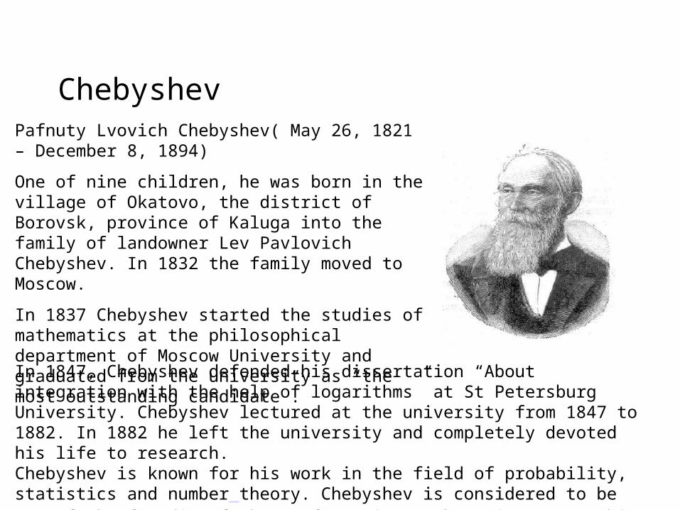
ChebyshevPafnuty Lvovich Chebyshev( May 26, 1821 – December 8, 1894)

One of nine children, he was born in the village of Okatovo, the district of Borovsk, province of Kaluga into the family of landowner Lev Pavlovich Chebyshev. In 1832 the family moved to Moscow.

In 1837 Chebyshev started the studies of mathematics at the philosophical department of Moscow University and graduated from the university as “the most outstanding candidate”.

In 1847, Chebyshev defended his dissertation “About integration with the help of logarithms” at St Petersburg University. Chebyshev lectured at the university from 1847 to 1882. In 1882 he left the university and completely devoted his life to research.Chebyshev is known for his work in the field of probability, statistics and number theory. Chebyshev is considered to be one of the founding fathers of Russian mathematics. Among his students were Aleksandr Lyapunov and Andrey Markov

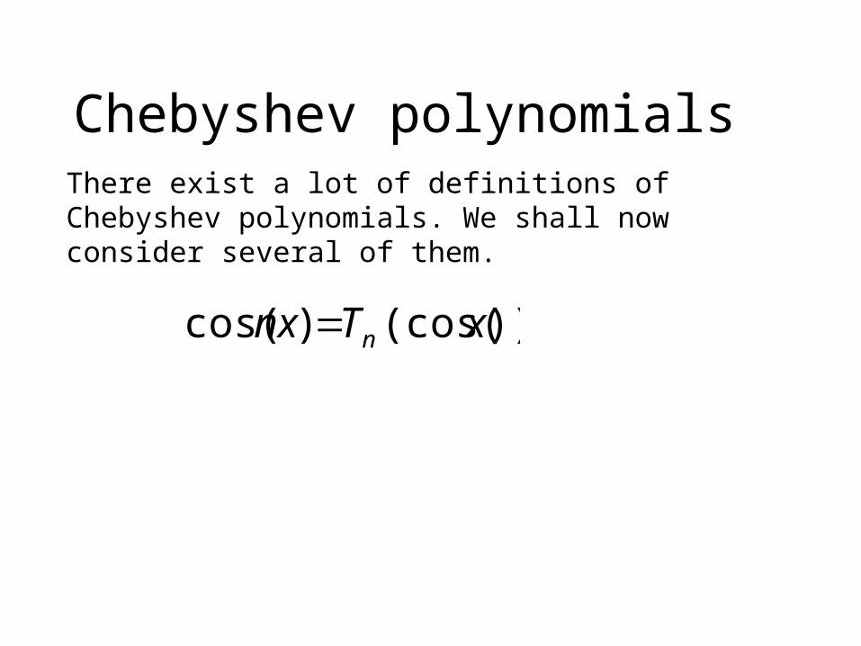
Chebyshev polynomialsThere exist a lot of definitions of Chebyshev polynomials. We shall now consider several of them.

))(cos()cos( xTnx n

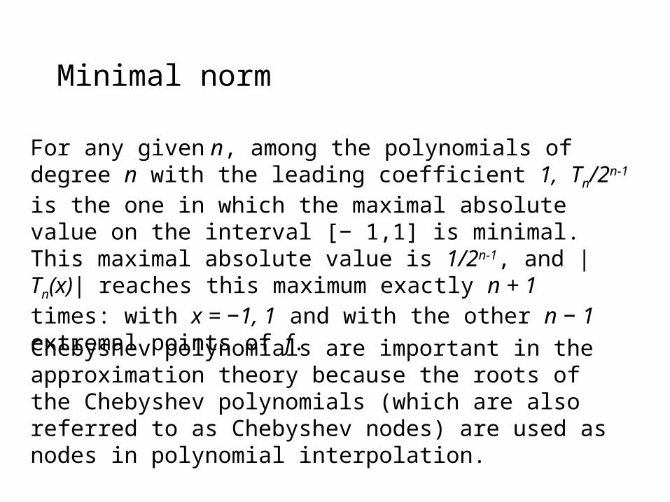
Minimal norm

Chebyshev polynomials are important in the approximation theory because the roots of the Chebyshev polynomials (which are also referred to as Chebyshev nodes) are used as nodes in polynomial interpolation.

For any given n, among the polynomials of degree n with the leading coefficient 1, Tn/2n-1 is the one in which the maximal absolute value on the interval [− 1,1] is minimal. This maximal absolute value is 1/2n-1, and |Tn(x)| reaches this maximum exactly n + 1 times: with x = −1, 1 and with the other n − 1 extremal points of f.

Basis of the space of polynomials

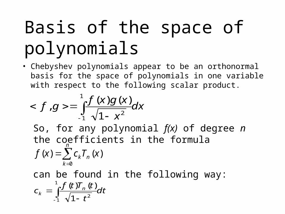
• Chebyshev polynomials appear to be an orthonormal basis for the space of polynomials in one variable with respect to the following scalar product.

dxx

xgxfgf

1

121

)()(,

So, for any polynomial f(x) of degree n the coefficients in the formula

can be found in the following way:

)()(0

xTcxfn

knk

dtt

tTtfc n

k

1

121

)()(

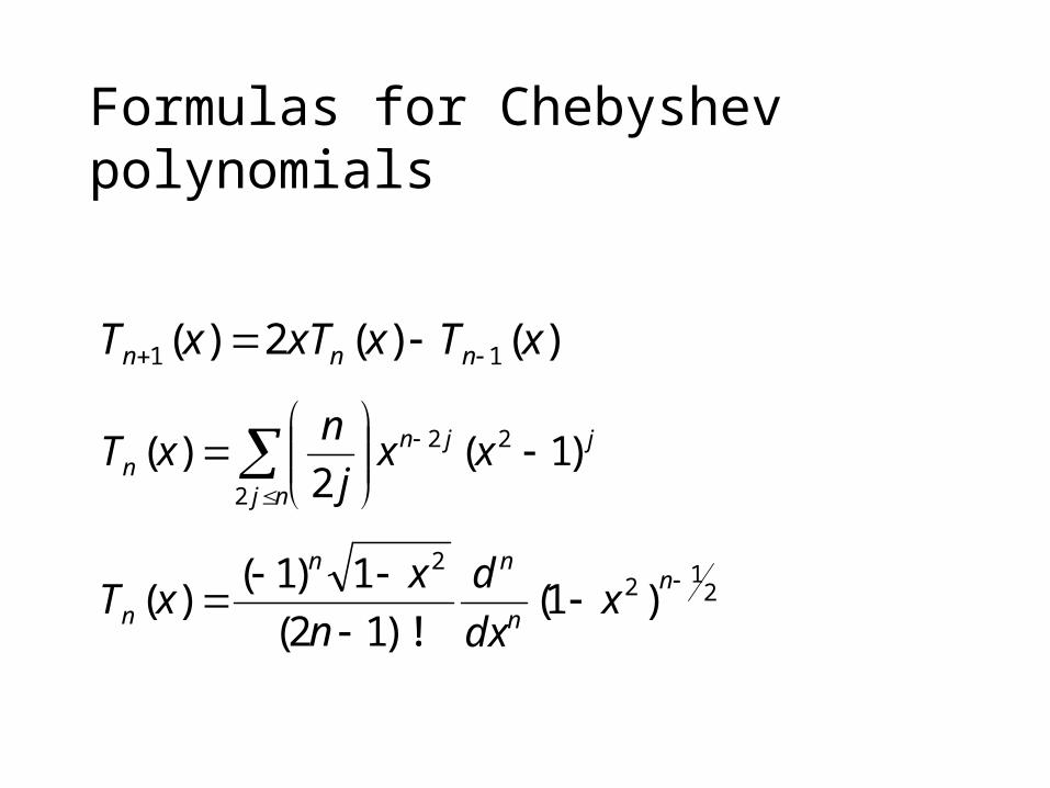
Formulas for Chebyshev polynomials

)()(2)( 11 xTxxTxT nnn

nj

jjnn xx

j

nxT

2

22 )1(2

)(

212

2

)1(!)!12(

1)1()(

n

n

nn

n xdx

d

n

xxT

Composition

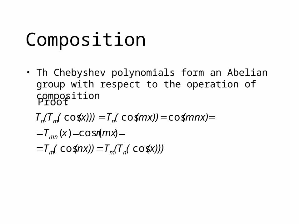
• Th Chebyshev polynomials form an Abelian group with respect to the operation of composition

(x)))((TT(nx))(T

nmxxT

(mnx)(mx))(T(x)))((TT

nmm

mn

nmn

coscos

)cos()(

coscoscos

:Proof

Generalizations

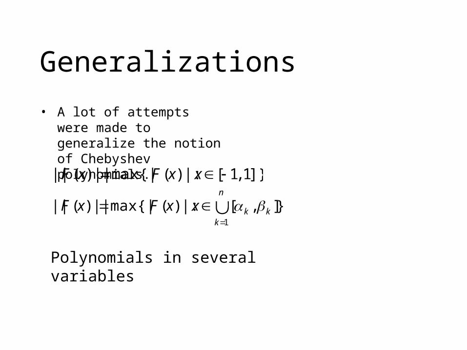
• A lot of attempts were made to generalize the notion of Chebyshev polynomials.

}],[|:)(max{|||)(||1

n

kkkxxFxF

Polynomials in several variables

]}1,1[|:)(max{|||)(|| xxFxF

Motivation

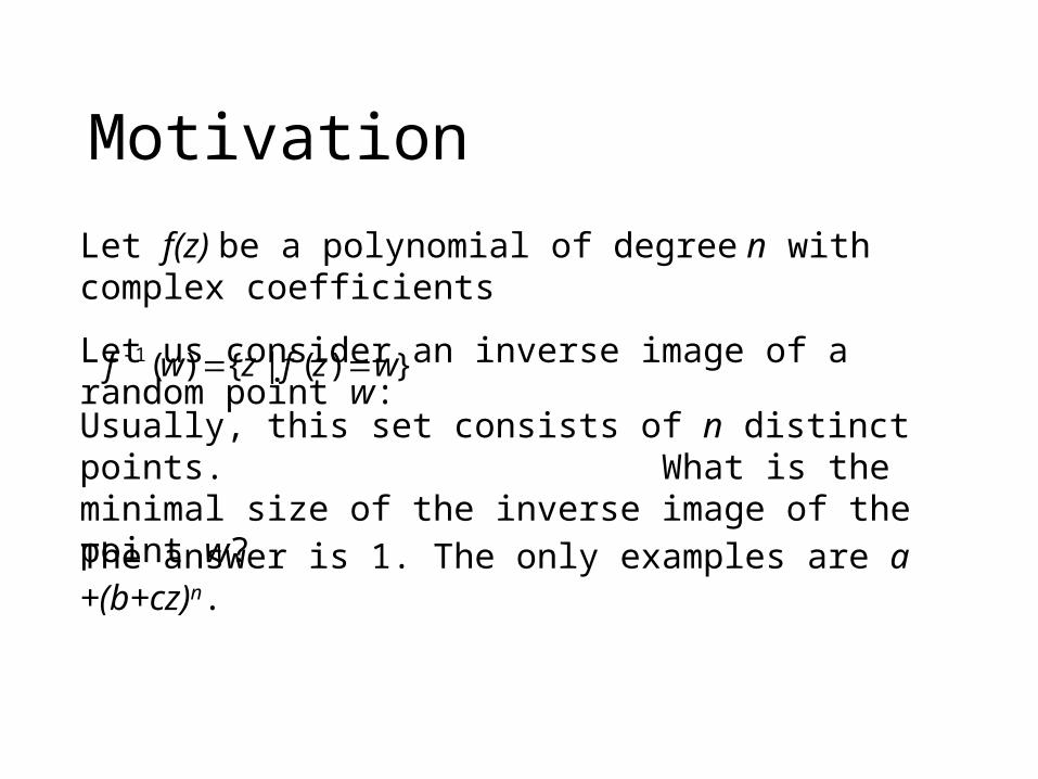
Let f(z) be a polynomial of degree n with complex coefficients

Let us consider an inverse image of a random point w:

The answer is 1. The only examples are a +(b+cz)n.

})(|{)(1 wzfzwf

Usually, this set consists of n distinct points. What is the minimal size of the inverse image of the point w?

MotivationAnd what is the minimal common size of the inverse image of two points w1 and w2?

The answer is n+1. But why?

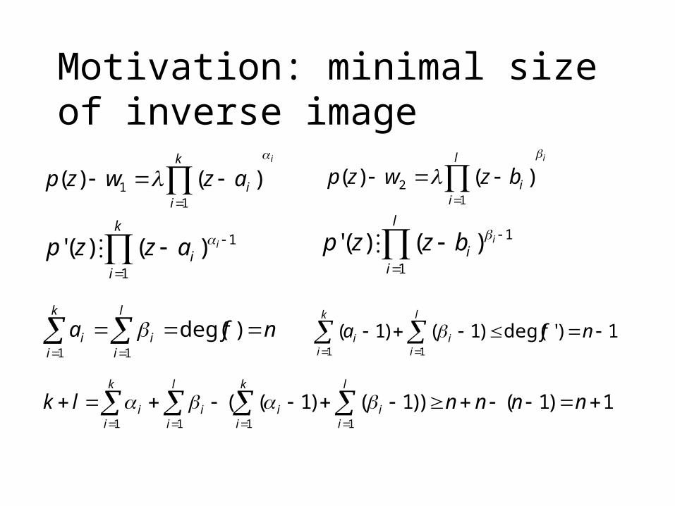
Motivation: minimal size of inverse image

il

iibzwzp

1

2 )()(ik

iiazwzp

1

1 )()(

nfal

ii

k

ii

)deg(11

k

ii

iazzp1

1)()('

l

ii

ibzzp1

1)()('

1)'deg()1()1(11

nfal

ii

k

ii

1)1())1()1((1111

nnnnlkl

ii

k

ii

l

ii

k

ii

Motivation

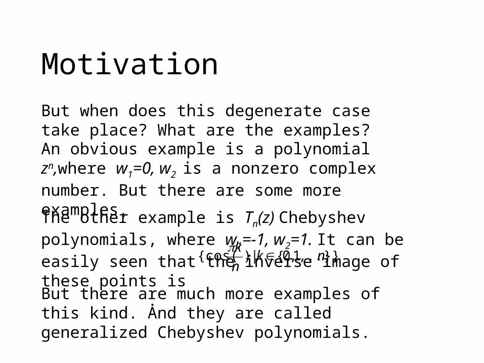
But when does this degenerate case take place? What are the examples?An obvious example is a polynomial zn,where w1=0, w2 is a nonzero complex number. But there are some more examples.

The other example is Tn(z) Chebyshev polynomials, where w1=-1, w2=1. It can be easily seen that the inverse image of these points is .}},...,1,0{|){cos( nk

n

k

But there are much more examples of this kind. And they are called generalized Chebyshev polynomials.

Motivation: minimal size of inverse image

il

iibzwzp

1

2 )()(ik

iiazwzp

1

1 )()(

nfal

ii

k

ii

)deg(11

k

ii

iazzp1

1)()('

l

ii

ibzzp1

1)()('

1)'deg()1()1(11

nfal

ii

k

ii

1)1())1()1((1111

nnnnlkl

ii

k

ii

l

ii

k

ii

Definition

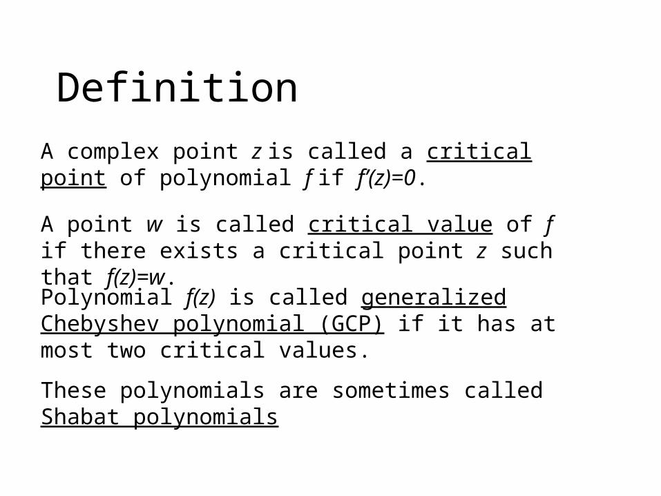
Polynomial f(z) is called generalized Chebyshev polynomial (GCP) if it has at most two critical values.

These polynomials are sometimes called Shabat polynomials

A complex point z is called a critical point of polynomial f if f’(z)=0.

A point w is called critical value of f if there exists a critical point z such that f(z)=w.

Certain properties of GCP

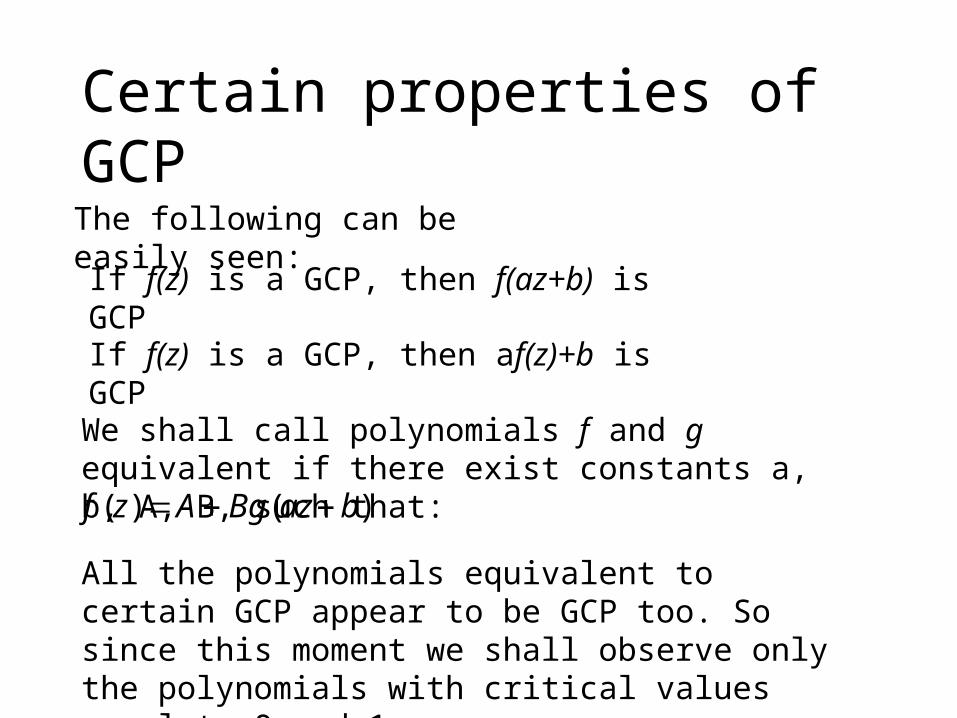
The following can be easily seen:

If f(z) is a GCP, then f(az+b) is GCP

If f(z) is a GCP, then af(z)+b is GCP

We shall call polynomials f and g equivalent if there exist constants a, b, A, B, such that:

)()( bazBgAzf

All the polynomials equivalent to certain GCP appear to be GCP too. So since this moment we shall observe only the polynomials with critical values equal to 0 and 1.

Geometric point of view

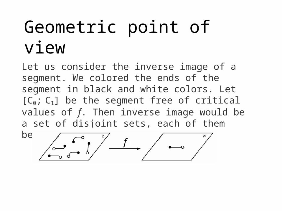
Let us consider the inverse image of a segment. We colored the ends of the segment in black and white colors. Let [C0; C1] be the segment free of critical values of f. Then inverse image would be a set of disjoint sets, each of them being homeomorphic to a segment.

f

Geometric point of view

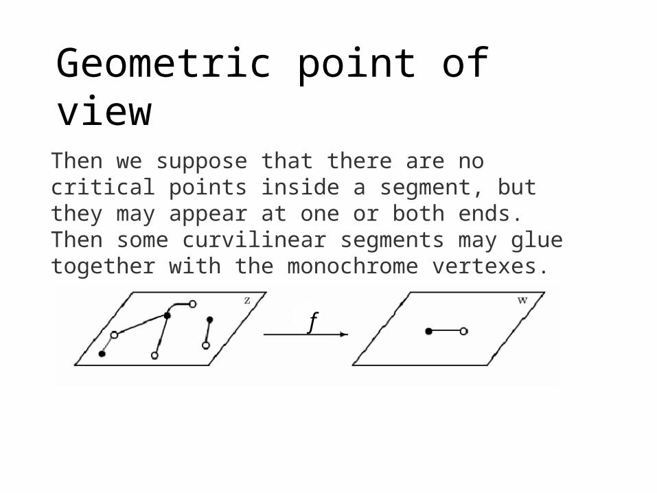
Then we suppose that there are no critical points inside a segment, but they may appear at one or both ends. Then some curvilinear segments may glue together with the monochrome vertexes.

f

Inverse image of a segment

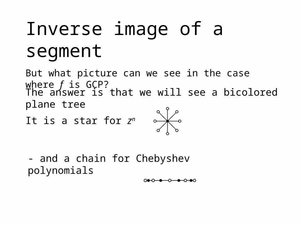
But what picture can we see in the case where f is GCP?

The answer is that we will see a bicolored plane tree

It is a star for zn

- and a chain for Chebyshev polynomials

Inverse image of a segment

Th For each GCP f the inverse image of a segment is a bicolored plane tree.

Proof:

In case of existence of a circuit our polynomial g takes only real values on the boundary of domain bounded by our circuit.

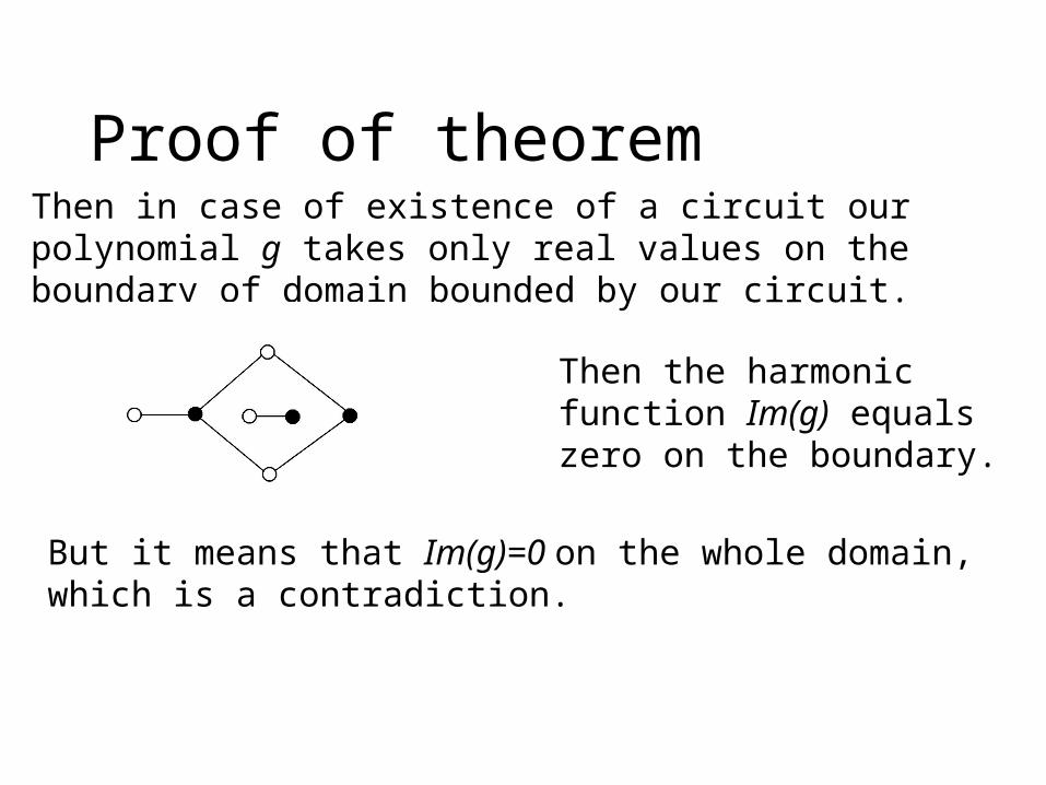
Proof of theoremThen in case of existence of a circuit our polynomial g takes only real values on the boundary of domain bounded by our circuit.

Then the harmonic function Im(g) equals zero on the boundary.

But it means that Im(g)=0 on the whole domain, which is a contradiction.

The inverse theoremTh For each bicolored plane tree T there exists a GCP such that the corresponding inverse image is T. Moreover, this GCP is unique up to the equivalence introduced above.

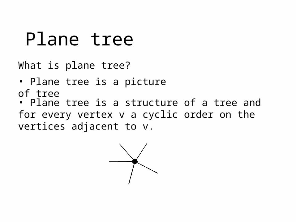
Plane treeWhat is plane tree?

• Plane tree is a picture of tree

• Plane tree is a structure of a tree and for every vertex v a cyclic order on the vertices adjacent to v.

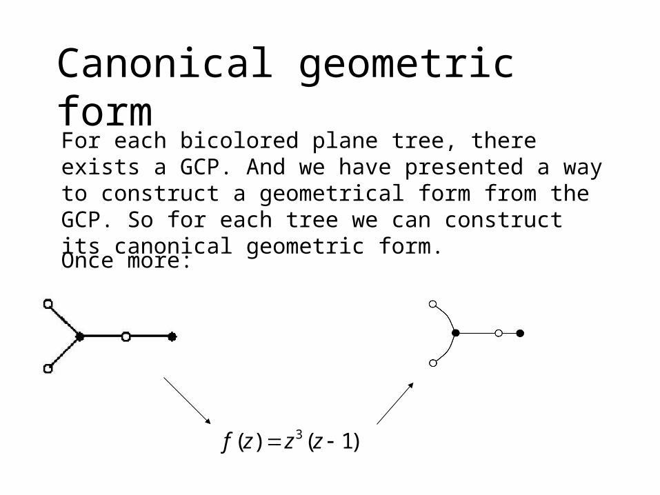
Canonical geometric form

)1()( 3 zzzf

For each bicolored plane tree, there exists a GCP. And we have presented a way to construct a geometrical form from the GCP. So for each tree we can construct its canonical geometric form.

Once more:

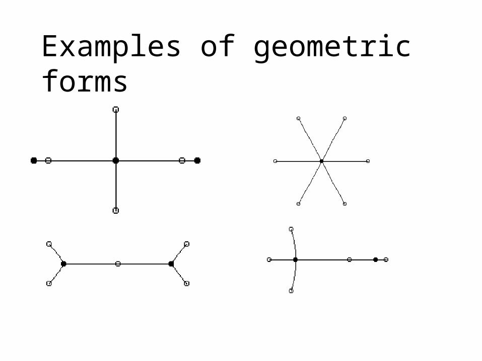
Examples of geometric forms

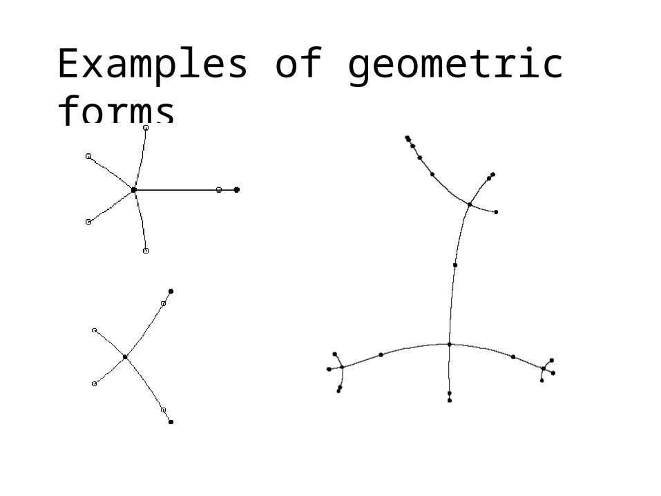
Examples of geometric forms

Construction of GCP

k

ii

iazzp1

)()(

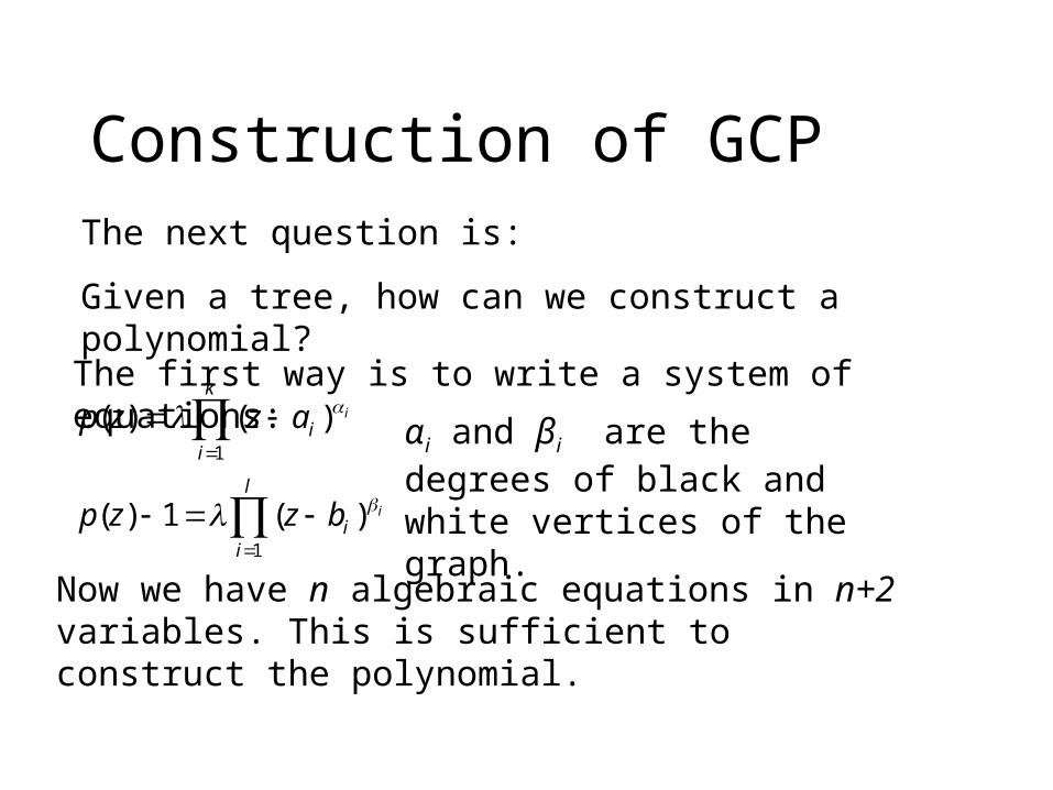
The next question is:

Given a tree, how can we construct a polynomial?

The first way is to write a system of equations:

l

ii

ibzzp1

)(1)(

Now we have n algebraic equations in n+2 variables. This is sufficient to construct the polynomial.

αi and βi are the degrees of black and white vertices of the graph.

Tree families

While constructing our GCP, we only used αi and βi, which are the degrees of black and white vertices of the graph.

But for each multiset of degrees there are a lot of trees with the same multisetset. All such trees form a family <α, β>, where α=(α1, α2, …αk), β =(β1, β2, … βn+1-k).

By solving the equations from the previous slide we can find all the polynomials which correspond to the trees of this family.

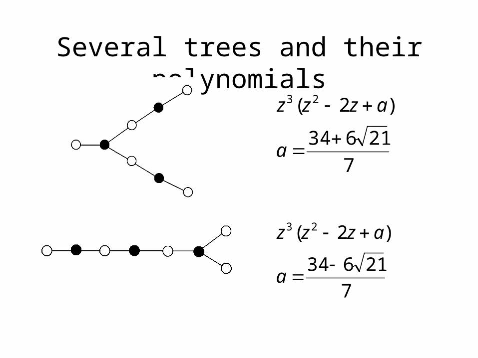
Several trees and their polynomials

7

21634

)2( 23

a

azzz

7

21634

)2( 23

a

azzz

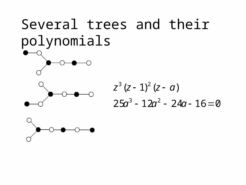
Several trees and their polynomials

016241225

)()1(23

23

aaa

azzz

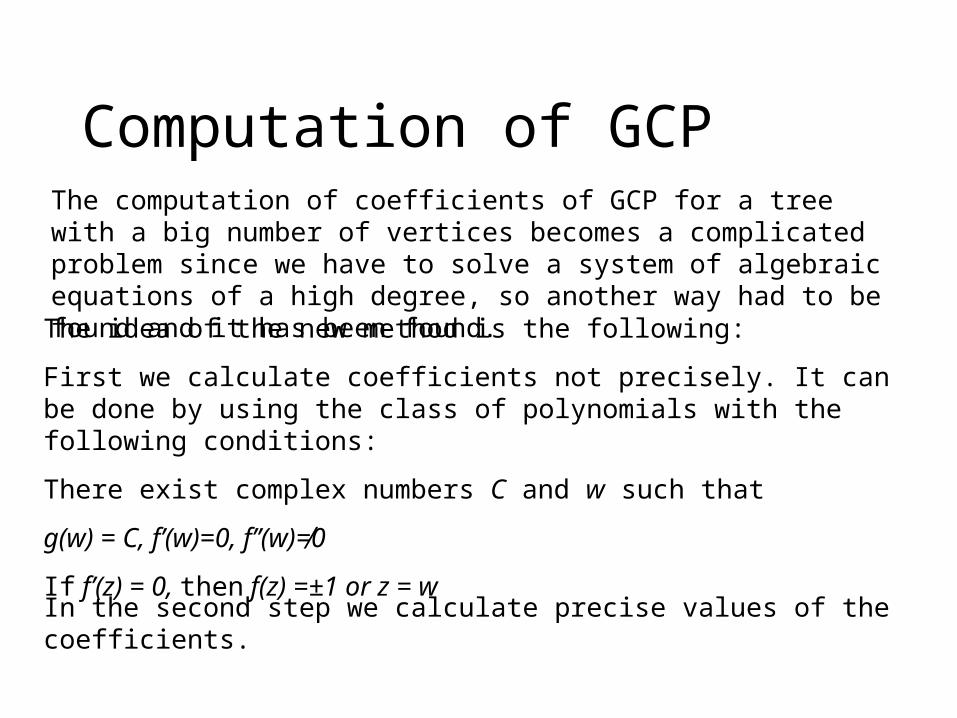
Computation of GCPThe computation of coefficients of GCP for a tree with a big number of vertices becomes a complicated problem since we have to solve a system of algebraic equations of a high degree, so another way had to be found and it has been found.

The idea of the new method is the following:

First we calculate coefficients not precisely. It can be done by using the class of polynomials with the following conditions:

There exist complex numbers C and w such that

g(w) = C, f’(w)=0, f’’(w)≠0

If f’(z) = 0, then f(z) =±1 or z = w

In the second step we calculate precise values of the coefficients.

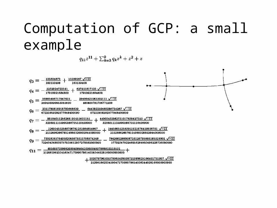
Computation of GCP: a small example

Galois group action on trees

k

ii

iazwzp1

1 )()(

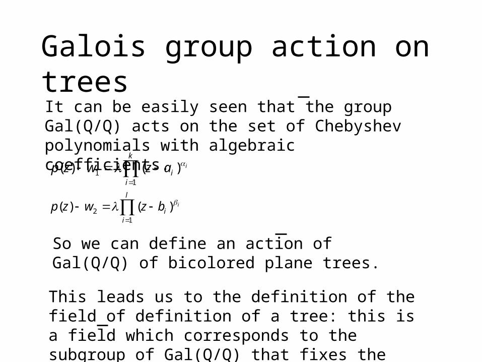
It can be easily seen that the group Gal(Q/Q) acts on the set of Chebyshev polynomials with algebraic coefficients.

l

ii

ibzwzp1

2 )()(

So we can define an action of Gal(Q/Q) of bicolored plane trees.

This leads us to the definition of the field of definition of a tree: this is a field which corresponds to the subgroup of Gal(Q/Q) that fixes the given tree.

GCP coefficientsBut what is the connection between the field of definition and generalized Chebyshev polynomials? The answer is given in the following theorem:

Th For any bicolored plane tree there exists a generalized Chebyshev polynomial whose coefficients belong to the field of definition of the tree.

Orbits vs families

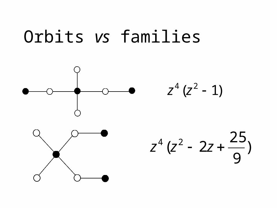
It can be easily seen that the action of Galois group on the tree does not change the multiset of valences of the tree.

So the orbit of a tree is a subset of its family. But do they coincide?

The answer is: not always.

Orbits vs families

)1( 24 zz

)9

252( 24 zzz

Composition of polynomials

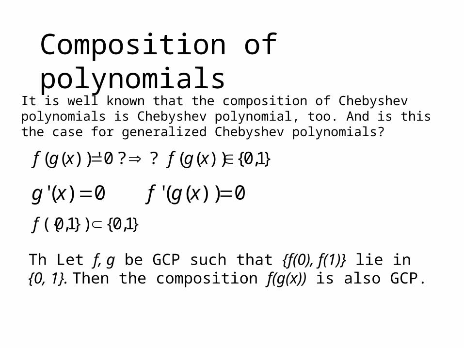
}1,0{))((??0))'(( xgfxgf

0))((' xgf0)(' xg

It is well known that the composition of Chebyshev polynomials is Chebyshev polynomial, too. And is this the case for generalized Chebyshev polynomials?

}1,0{})1,0({ f

Th Let f, g be GCP such that {f(0), f(1)} lie in {0, 1}. Then the composition f(g(x)) is also GCP.

Composition of treesLet us imagine that we have two trees T1 and T2. Their polynomials are f1 and f2. And we need to construct a tree which corresponds to f1◦f2. Do we have to calculate f1 and f2, find their composition and then construct a tree or there is a direct way?

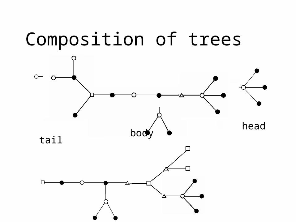
Composition of trees

head

tailbody

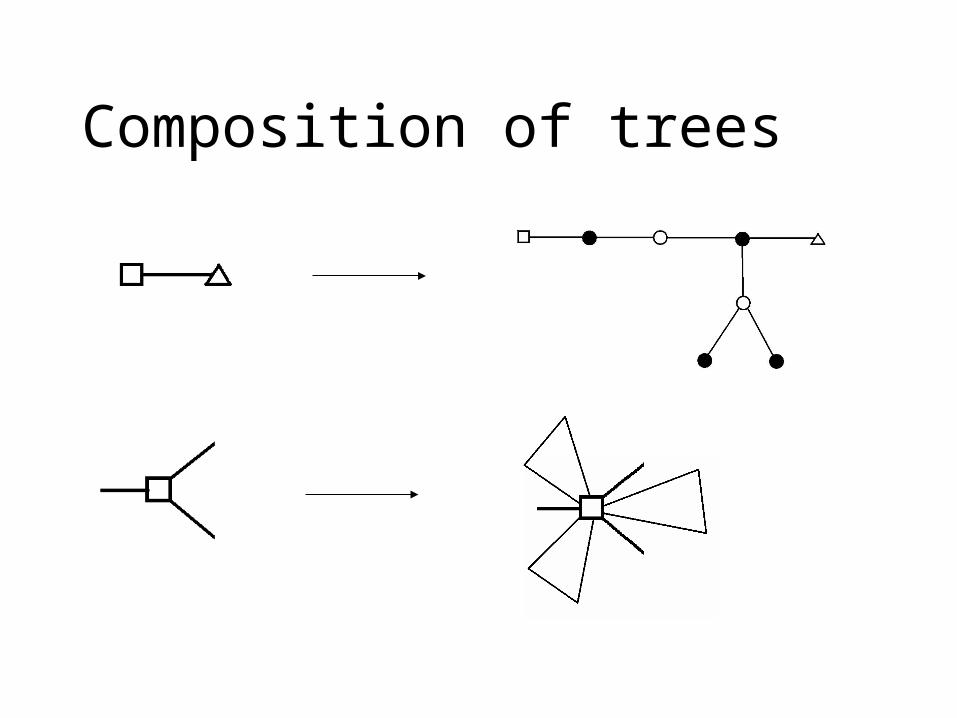
Composition of trees

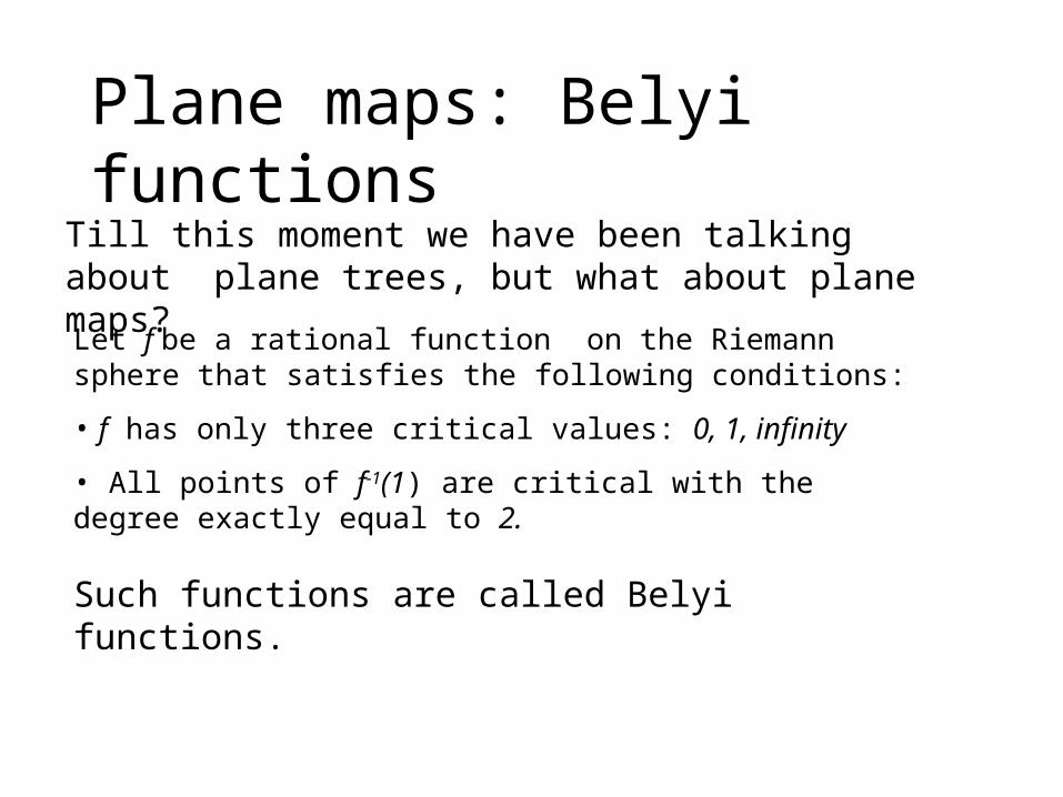
Plane maps: Belyi functionsTill this moment we have been talking about plane trees, but what about plane maps?

Let f be a rational function on the Riemann sphere that satisfies the following conditions:

• f has only three critical values: 0, 1, infinity

• All points of f-1(1) are critical with the degree exactly equal to 2.

Such functions are called Belyi functions.

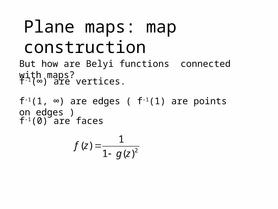
Plane maps: map construction

But how are Belyi functions connected with maps?

f-1(∞) are vertices.

f-1(1, ∞) are edges ( f-1(1) are points on edges )

f-1(0) are faces

2)(1

1)(

zgzf