23 11

Article 12.4.8Journal of Integer Sequences, Vol. 15 (2012),2

3

6

1

47

Generalized Narayana Polynomials,

Riordan Arrays, and Lattice Paths

Paul BarrySchool of Science

Waterford Institute of TechnologyIreland

pbarry@wit.ie

Aoife HennessyDepartment of Computing, Mathematics and Physics

Waterford Institute of TechnologyIreland

aoife.hennessy@gmail.com

Abstract

We study a family of polynomials in two variables, identifying them as the moments

of a two-parameter family of orthogonal polynomials. The coefficient array of these

orthogonal polynomials is shown to be an ordinary Riordan array. We express the gen-

erating function of the sequence of polynomials under study as a continued fraction,

and determine the corresponding Hankel transform. An alternative characterization

of the polynomials in terms of a related Riordan array is also given. This Riordan

array is associated with Lukasiewicz paths. The special form of the production ma-

trices is exhibited in both cases. This allows us to produce a bijection from a set of

colored Lukasiewicz paths to a set of colored Motzkin paths. The polynomials studied

generalize the notion of Narayana polynomial.

1 Introduction

In this note, we shall be concerned with the family of bivariate polynomials defined by

Qn(r, s) =n∑

k=0

k∑

j=0

(

n

j

)(

n − j

2(k − j)

)

ak−j(s)rk,

1

where

an(s) =n∑

k=0

(

2n − k − 1

n − k

)

k + 0n+k

n + 0nksk.

Our main goal is to characterize Qn(r, s) as the moment sequence of a family of orthogonalpolynomials, and in so doing also show that the sequence Qn(r, s) has Hankel transformhn(r, s) = det(Qi+j(r, s))0≤i,j≤n [26] given by

hn(r, s) = snr(n+1

2 ).

Examples of these sequences include the shifted Catalan numbers Qn(1, 1), the centralbinomial coefficients Qn(1, 2), the central Delannoy numbers Qn(2, 2), and many other se-quences that are documented in the On Line Encyclopedia of Integer Sequences [31, 32].

We use the production matrix of a particular Riordan array to establish the existenceof a family of orthogonal polynomials for which the generalized Narayana polynomials aremoments. We find it interesting to look at a closely related Riordan array, again withthe generalized Narayana polynomials as elements of the first column, but where now theproduction matrix is not tri-diagonal. It does however have a structure that is interesting inits own right. The Hankel transform of the row sum sequence of this second Riordan arrayis also interesting to study.

2 Preliminaries on integer sequences, Riordan arrays

and Hankel transforms

For an integer sequence an, that is, an element of ZN, the power series f(x) =

∑∞n=0 anx

n

is called the ordinary generating function or g.f. of the sequence. an is thus the coefficientof xn in this series. We denote this by an = [xn]f(x). For instance, Fn = [xn] x

1−x−x2 is

the n-th Fibonacci number A000045, while Cn = [xn]1−√

1−4x

2xis the n-th Catalan number

A000108. We use the notation 0n = [xn]1 for the sequence 1, 0, 0, 0, . . . , A000007. Thus0n = [n = 0] = δn,0 =

(

0n

)

. Here, we have used the Iverson bracket notation [19], defined by[P ] = 1 if the proposition P is true, and [P ] = 0 if P is false.

For a power series f(x) =∑∞

n=0 anxn with f(0) = 0 we define the reversion or composi-

tional inverse of f to be the power series f(x) such that f(f(x)) = x.For a lower triangular matrix (an,k)n,k≥0 the row sums give the sequence with general

term∑n

k=0 an,k.The Riordan group [30, 33], is a set of infinite lower-triangular integer matrices, where

each matrix is defined by a pair of generating functions g(x) = 1 + g1x + g2x2 + · · · and

f(x) = f1x + f2x2 + · · · where f1 6= 0 [33]. We assume in addition that f1 = 1 in what

follows. The associated matrix is the matrix whose i-th column is generated by g(x)f(x)i

(the first column being indexed by 0). The matrix corresponding to the pair g, f is denotedby (g, f) or R(g, f). The group law is then given by

(g, f) · (h, l) = (g, f)(h, l) = (g(h ◦ f), l ◦ f).

2

The identity for this law is I = (1, x) and the inverse of (g, f) is (g, f)−1 = (1/(g ◦ f), f)where f is the compositional inverse of f .

If M is the matrix (g, f), and a = (a0, a1, . . .)′ is an integer sequence with ordinary gener-

ating function A (x), then the sequence Ma has ordinary generating function g(x)A(f(x)).The (infinite) matrix (g, f) can thus be considered to act on the ring of integer sequencesZ

N by multiplication, where a sequence is regarded as a (infinite) column vector. We canextend this action to the ring of power series Z[[x]] by

(g, f) : A(x) 7→ (g, f) · A(x) = g(x)A(f(x)).

Example 1. The so-called binomial matrix B is the element ( 11−x

, x1−x

) of the Riordan

group. It has general element(

n

k

)

, and hence as an array coincides with Pascal’s triangle.More generally, Bm is the element ( 1

1−mx, x

1−mx) of the Riordan group, with general term

(

n

k

)

mn−k. It is easy to show that the inverse B−m of Bm is given by ( 11+mx

, x1+mx

).

For an invertible matrix L, its production matrix (also called its Stieltjes matrix) [15, 16]is the matrix

PL = L−1L,

where L is the matrix L with its first row removed. A Riordan array L is the inverse of thecoefficient array of a family of orthogonal polynomials if and only if PL is tri-diagonal [7, 8].Necessarily, the Jacobi coefficients of these orthogonal polynomials are then constant. Suchtypes of polynomials have been studied in many contexts, including orthogonal polynomials[34, 18, 1, 2], random walks [23, 20], group theory [13], non-commutative probability [29, 3,11], and the study of random matrices [14].

An important feature of Riordan arrays is that they have a number of sequence charac-terizations [12, 21]. The simplest of these is as follows.

Proposition 2. [21, Theorem 2.1, Theorem 2.2] Let D = [dn,k] be an infinite triangularmatrix. Then D is a Riordan array if and only if there exist two sequences A = [a0, a1, a2, . . .]and Z = [z0, z1, z2, . . .] with a0 6= 0, z0 6= 0 such that

• dn+1,k+1 =∑∞

j=0 ajdn,k+j, (k, n = 0, 1, . . .)

• dn+1,0 =∑∞

j=0 zjdn,j, (n = 0, 1, . . .).

The coefficients a0, a1, a2, . . . and z0, z1, z2, . . . are called the A-sequence and the Z-sequence of the Riordan array L = (g(x), f(x)), respectively. Letting A(x) be the generatingfunction of the A-sequence and Z(x) be the generating function of the Z-sequence, we have

A(x) =x

f(x), Z(x) =

1

f(x)

(

1 − 1

g(f(x))

)

. (1)

The first column of PL is then generated by Z(x), while the k-th column is generated byxk−1A(x) (taking the first column to be indexed by 0).

For a given sequence an, the Hankel transform [26] of an is the sequence det(ai+j)0≤i,j≤n.The Hankel transforms we shall be interested in will all be related to orthogonal polynomials,

3

which in turn will be related to lattice paths [17, 35]. A lattice path [27] is a sequence ofvertices in the integer lattice Z

2. A pair of consecutive vertices is called a step of the path.The height of a step is given by the y-value of the first vertex. A valuation is an integerfunction on the set of possible steps of Z

2 × Z2. A valuation of a path is the product of

the valuations of its steps. We concern ourselves with Motzkin paths, k-colored Motzkinpaths [4] and Lukasiewicz paths [35], which are defined below. A path of length n beginsat (0, 0) and ends at (n, 0). The valuations will be independent of the x-coordinates of thepoints, therefore the x-coordinates are redundant and we can represent a path π by thesequence of its y-coordinates π = (π(0) · · ·π(n)).

Definition 3. A path π = (π(0) · · ·π(n)) is a Motzkin path [27] if it satisfies the followingconditions

1. The elementary steps can be north-east, east and south-east.

2. Steps never go below the x axis.

3. π(0) = (0, 0) and π(n) = (n, 0)

If the east steps are labelled by k colors we obtain the k-colored Motzkin paths.

Definition 4. A path π = (π(0) · · ·π(n)) is a Lukasiewicz path [27] if it satisfies the followingconditions

1. The elementary steps can be north - east and east as those in Motzkin paths.

2. In addition south-east steps from level k can fall to any level above or on the x axis,and are denoted as λk,l and referred to as Lukasiewicz steps, where k is the startingpoint of the south-east step and l the level where the step ends.

3. Steps never go below the x axis.

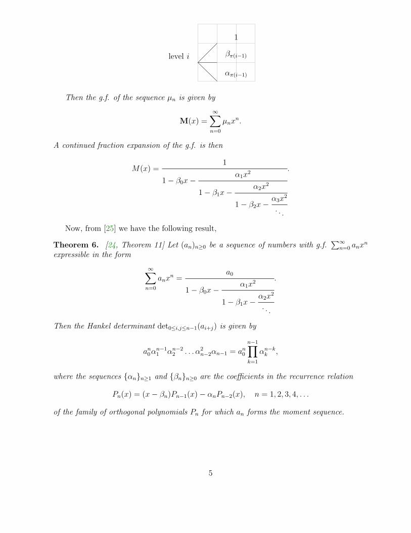
Theorem 5. [27, Theorem 2.3] Let

µn =∑

π∈M

v(π)

where the sum is over the set of Motzkin paths π = (π(0) · · ·π(n)) of length n. Here π(j) isthe level after the jth step, and the valuation of a path is the product of the valuations of itssteps v(π) =

∏n

i=1 vi where

vi = v(π(i − 1), π(i)) =

1, if the ith step rises;

βπ(i−1), if the ith step is horizontal;

απ(i−1), if the ith step falls.

4

1

level i βπ(i−1)

απ(i−1)

Then the g.f. of the sequence µn is given by

M(x) =∞∑

n=0

µnxn.

A continued fraction expansion of the g.f. is then

M(x) =1

1 − β0x −α1x

2

1 − β1x −α2x

2

1 − β2x −α3x

2

. . .

.

Now, from [25] we have the following result,

Theorem 6. [24, Theorem 11] Let (an)n≥0 be a sequence of numbers with g.f.∑∞

n=0 anxn

expressible in the form

∞∑

n=0

anxn =

a0

1 − β0x −α1x

2

1 − β1x −α2x

2

. . .

.

Then the Hankel determinant det0≤i,j≤n−1(ai+j) is given by

an0α

n−11 αn−2

2 . . . α2n−2αn−1 = an

0

n−1∏

k=1

αn−kk ,

where the sequences {αn}n≥1 and {βn}n≥0 are the coefficients in the recurrence relation

Pn(x) = (x − βn)Pn−1(x) − αnPn−2(x), n = 1, 2, 3, 4, . . .

of the family of orthogonal polynomials Pn for which an forms the moment sequence.

5

3 Generalized Narayana polynomials

The sequence an(s) =∑n

k=0

(

2n−k−1n−k

)

k+0n+k

n+0nk sk has generating function [10]

gs(x) =1

1 − sxc(x)= (1, xc(x)) · 1

1 − sx,

where c(x) = 1−√

1−4x

2xis the generating function of the Catalan numbers, and (1, xc(x)) is

the Riordan array [30] whose k-th column has generating function (xc(x))k [10]. Since c(x)has continued fraction expansion

c(x) =1

1 −x

1 −x

1 − · · ·

,

the generating function gs(x) has expansion

gs(x) =1

1 −sx

1 −x

1 −x

1 − · · ·

.

The matrix with general term

Nn,k(s) =k∑

j=0

(

n

j

)(

n − j

2(k − j)

)

ak−j(s)

is the generalized Narayana triangle [5] defined by the sequence an(s), and the polynomialsQn(r, s) thus represent generalized Narayana polynomials. The Narayana triangle A001263with general term

1

k + 1

(

n + 1

k

)(

n

k

)

corresponds to s = 1. For s = 2 we get the number triangle with general term(

n

k

)2A008459.

Proposition 7. The generating function of the polynomials Qn(r, s) =∑n

k=0 Nn,k(s)rk isgiven by

gQ(x) =1

1 − (r + 1)x −srx2

1 − (r + 1)x −rx2

1 − (r + 1)x −rx2

1 − · · ·

.

6

Proof. See Theorem 21, [5].

Corollary 8. The Hankel transform of Qn(r, s) is given by

hn = snr(n+1

2 ).

Proof. This follows from [24, 25].

We know [6] that the Narayana polynomials∑n

k=01

k+1

(

n

k

)(

n+1k

)

rk can be characterized asbeing the first column elements of the inverse Riordan array

(

1

1 + (r + 1)x + rx2,

x

1 + (r + 1)x + rx2

)−1

.

The following proposition generalizes this result, by providing a characterization of the poly-nomials Qn(r, s) in terms of Riordan arrays.

Proposition 9. The polynomials Qn(r, s) are given by the terms of the first column of theRiordan array

L =

(

1 + r(1 − s)x2

1 + (r + 1)x + rx2,

x

1 + (r + 1)x + rx2

)−1

.

Proof. We can express gQ(x) in closed form by noticing that

gQ(x) =1

1 − (r + 1)x − srx2v,

where v is the solution of the equation

v =1

1 − (r + 1)x − rx2v.

(The function v is the generating function of the Narayana triangle). We find that

gQ(x) =2

s√

x2(r − 1)2 − 2x(r + 1) + 1 + (x(r + 1) − 1)(s − 2).

Standard Riordan array techniques [7] now show that this is equal to the generating

function of the first column of the inverse array(

1+r(1−s)x2

1+(r+1)x+rx2 ,x

1+(r+1)x+rx2

)−1

.

Note that we can also express gQ(x) as follows.

gQ(x) =s√

x2(r − 1)2 − 2x(r + 1) + 1 + (2 − s)(x(r + 1) − 1)

2(x2(r2(s − 1) − r(s2 − 2s + 2) + s − 1) + (s − 1)(1 − 2x(r + 1))).

We have

L =

(

gQ(x),1 − x(r + 1) −

√

1 − 2x(r + 1) + x2(r − 1)2

2rx

)

.

7

Corollary 10. The polynomials Qn(r, s) are the moments of the family of orthogonal poly-nomials Pn(x) that satisfy the recurrence

Pn(x) = (x − (r + 1))Pn−1(x) − rPn−2(x), n > 2,

P0(x) = 1, P1(x) = x − (r + 1), P2(x) = (x − (r + 1))P1(x) − srP0(x) = x2 − 2(r + 1)x +r2 + r(2 − s) + 1.

Proof. We need to show [7, 8] that the production matrix [15, 16] of

L =

(

1 + r(1 − s)x2

1 + (r + 1)x + rx2,

x

1 + (r + 1)x + rx2

)−1

is tri-diagonal. Standard Riordan array techniques show that this is so, with form

PL =

r + 1 1 0 0 0 0 · · ·sr r + 1 1 0 0 0 · · ·0 r r + 1 1 0 0 · · ·0 0 r r + 1 1 0 · · ·0 0 0 r r + 1 1 · · ·0 0 0 0 r r + 1 · · ·...

......

......

.... . .

.

The three-term recurrence coefficients for Pn(x) can be read from PL.

Corollary 11. The Hankel transform of Qn(r, s) is given by

hn(r, s) = snr(n+1

2 ).

Proof. This is a direct consequence of the form of gQ; equivalently it is derived from theform of the production matrix above.

We note that Qn(r, j/r) is an integer sequence for 0 ≤ j ≤ r−1. For instance, Qn(2, 1/2)is the sequence that begins

1, 3, 10, 36, 138, 558, 2362, 10398, 47326, 221562, . . .

It has generating function

1

1 − 3x −x2

1 − 3x −2x2

1 − 3x −2x2

1 − · · ·

.

8

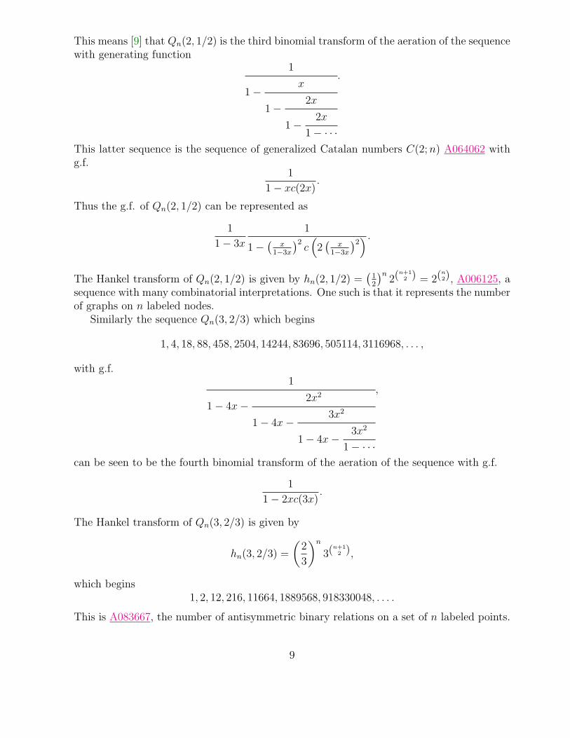
This means [9] that Qn(2, 1/2) is the third binomial transform of the aeration of the sequencewith generating function

1

1 −x

1 −2x

1 −2x

1 − · · ·

.

This latter sequence is the sequence of generalized Catalan numbers C(2; n) A064062 withg.f.

1

1 − xc(2x).

Thus the g.f. of Qn(2, 1/2) can be represented as

1

1 − 3x

1

1 −(

x1−3x

)2c(

2(

x1−3x

)2) .

The Hankel transform of Qn(2, 1/2) is given by hn(2, 1/2) =(

12

)n2(n+1

2 ) = 2(n

2), A006125, asequence with many combinatorial interpretations. One such is that it represents the numberof graphs on n labeled nodes.

Similarly the sequence Qn(3, 2/3) which begins

1, 4, 18, 88, 458, 2504, 14244, 83696, 505114, 3116968, . . . ,

with g.f.1

1 − 4x −2x2

1 − 4x −3x2

1 − 4x −3x2

1 − · · ·

,

can be seen to be the fourth binomial transform of the aeration of the sequence with g.f.

1

1 − 2xc(3x).

The Hankel transform of Qn(3, 2/3) is given by

hn(3, 2/3) =

(

2

3

)n

3(n+1

2 ),

which begins1, 2, 12, 216, 11664, 1889568, 918330048, . . . .

This is A083667, the number of antisymmetric binary relations on a set of n labeled points.

9

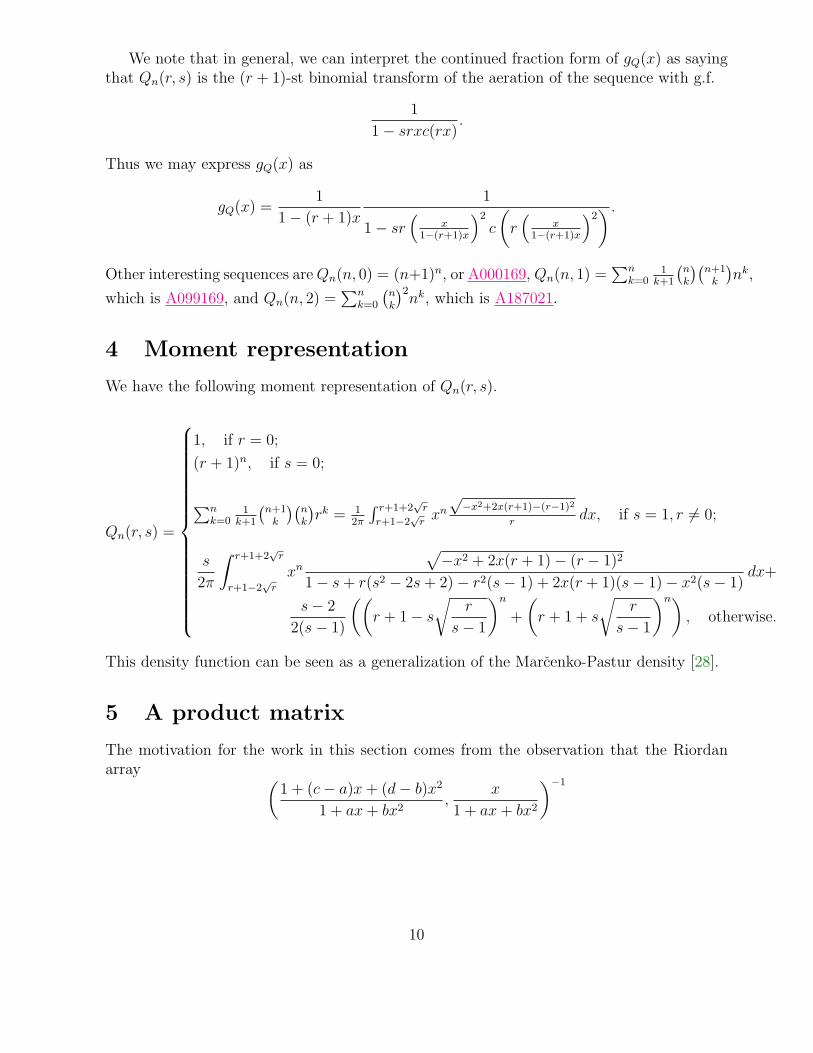
We note that in general, we can interpret the continued fraction form of gQ(x) as sayingthat Qn(r, s) is the (r + 1)-st binomial transform of the aeration of the sequence with g.f.

1

1 − srxc(rx).

Thus we may express gQ(x) as

gQ(x) =1

1 − (r + 1)x

1

1 − sr(

x1−(r+1)x

)2

c

(

r(

x1−(r+1)x

)2) .

Other interesting sequences are Qn(n, 0) = (n+1)n, or A000169, Qn(n, 1) =∑n

k=01

k+1

(

n

k

)(

n+1k

)

nk,

which is A099169, and Qn(n, 2) =∑n

k=0

(

n

k

)2nk, which is A187021.

4 Moment representation

We have the following moment representation of Qn(r, s).

Qn(r, s) =

1, if r = 0;

(r + 1)n, if s = 0;

∑n

k=01

k+1

(

n+1k

)(

n

k

)

rk = 12π

∫ r+1+2√

r

r+1−2√

rxn

√−x2+2x(r+1)−(r−1)2

rdx, if s = 1, r 6= 0;

s

2π

∫ r+1+2√

r

r+1−2√

r

xn

√

−x2 + 2x(r + 1) − (r − 1)2

1 − s + r(s2 − 2s + 2) − r2(s − 1) + 2x(r + 1)(s − 1) − x2(s − 1)dx+

s − 2

2(s − 1)

((

r + 1 − s

√

r

s − 1

)n

+

(

r + 1 + s

√

r

s − 1

)n)

, otherwise.

This density function can be seen as a generalization of the Marcenko-Pastur density [28].

5 A product matrix

The motivation for the work in this section comes from the observation that the Riordanarray

(

1 + (c − a)x + (d − b)x2

1 + ax + bx2,

x

1 + ax + bx2

)−1

10

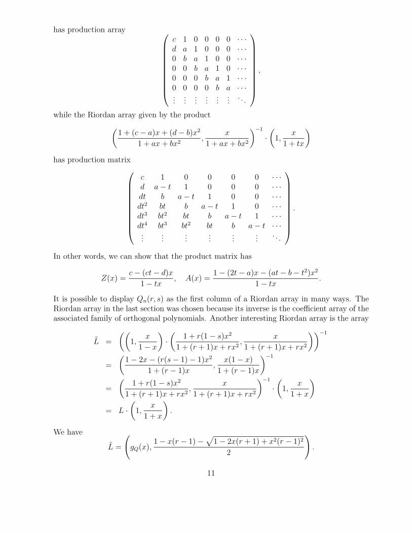
has production array

c 1 0 0 0 0 · · ·d a 1 0 0 0 · · ·0 b a 1 0 0 · · ·0 0 b a 1 0 · · ·0 0 0 b a 1 · · ·0 0 0 0 b a · · ·...

......

......

.... . .

,

while the Riordan array given by the product

(

1 + (c − a)x + (d − b)x2

1 + ax + bx2,

x

1 + ax + bx2

)−1

·(

1,x

1 + tx

)

has production matrix

c 1 0 0 0 0 · · ·d a − t 1 0 0 0 · · ·dt b a − t 1 0 0 · · ·dt2 bt b a − t 1 0 · · ·dt3 bt2 bt b a − t 1 · · ·dt4 bt3 bt2 bt b a − t · · ·...

......

......

.... . .

.

In other words, we can show that the product matrix has

Z(x) =c − (ct − d)x

1 − tx, A(x) =

1 − (2t − a)x − (at − b − t2)x2

1 − tx.

It is possible to display Qn(r, s) as the first column of a Riordan array in many ways. TheRiordan array in the last section was chosen because its inverse is the coefficient array of theassociated family of orthogonal polynomials. Another interesting Riordan array is the array

L =

((

1,x

1 − x

)

·(

1 + r(1 − s)x2

1 + (r + 1)x + rx2,

x

1 + (r + 1)x + rx2

))−1

=

(

1 − 2x − (r(s − 1) − 1)x2

1 + (r − 1)x,

x(1 − x)

1 + (r − 1)x

)−1

=

(

1 + r(1 − s)x2

1 + (r + 1)x + rx2,

x

1 + (r + 1)x + rx2

)−1

·(

1,x

1 + x

)

= L ·(

1,x

1 + x

)

.

We have

L =

(

gQ(x),1 − x(r − 1) −

√

1 − 2x(r + 1) + x2(r − 1)2

2

)

.

11

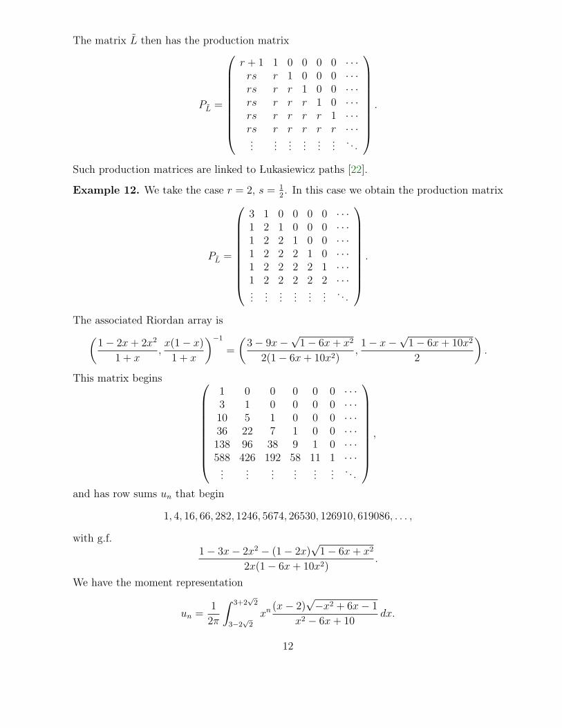
The matrix L then has the production matrix

PL =

r + 1 1 0 0 0 0 · · ·rs r 1 0 0 0 · · ·rs r r 1 0 0 · · ·rs r r r 1 0 · · ·rs r r r r 1 · · ·rs r r r r r · · ·...

......

......

.... . .

.

Such production matrices are linked to Lukasiewicz paths [22].

Example 12. We take the case r = 2, s = 12. In this case we obtain the production matrix

PL =

3 1 0 0 0 0 · · ·1 2 1 0 0 0 · · ·1 2 2 1 0 0 · · ·1 2 2 2 1 0 · · ·1 2 2 2 2 1 · · ·1 2 2 2 2 2 · · ·...

......

......

.... . .

.

The associated Riordan array is

(

1 − 2x + 2x2

1 + x,x(1 − x)

1 + x

)−1

=

(

3 − 9x −√

1 − 6x + x2

2(1 − 6x + 10x2),1 − x −

√1 − 6x + 10x2

2

)

.

This matrix begins

1 0 0 0 0 0 · · ·3 1 0 0 0 0 · · ·10 5 1 0 0 0 · · ·36 22 7 1 0 0 · · ·138 96 38 9 1 0 · · ·588 426 192 58 11 1 · · ·

......

......

......

. . .

,

and has row sums un that begin

1, 4, 16, 66, 282, 1246, 5674, 26530, 126910, 619086, . . . ,

with g.f.1 − 3x − 2x2 − (1 − 2x)

√1 − 6x + x2

2x(1 − 6x + 10x2).

We have the moment representation

un =1

2π

∫ 3+2√

2

3−2√

2

xn (x − 2)√−x2 + 6x − 1

x2 − 6x + 10dx.

12

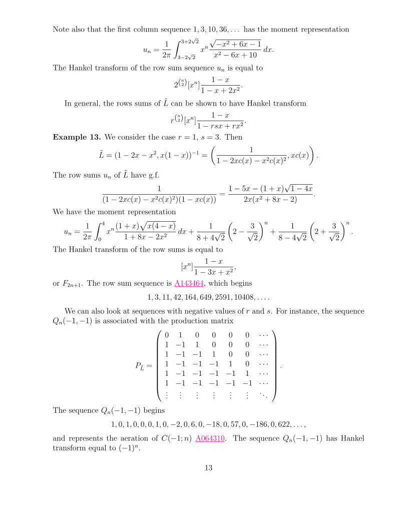
Note also that the first column sequence 1, 3, 10, 36, . . . has the moment representation

un =1

2π

∫ 3+2√

2

3−2√

2

xn

√−x2 + 6x − 1

x2 − 6x + 10dx.

The Hankel transform of the row sum sequence un is equal to

2(n

2)[xn]1 − x

1 − x + 2x2.

In general, the rows sums of L can be shown to have Hankel transform

r(n

2)[xn]1 − x

1 − rsx + rx2.

Example 13. We consider the case r = 1, s = 3. Then

L = (1 − 2x − x2, x(1 − x))−1 =

(

1

1 − 2xc(x) − x2c(x)2, xc(x)

)

.

The row sums un of L have g.f.

1

(1 − 2xc(x) − x2c(x)2)(1 − xc(x))=

1 − 5x − (1 + x)√

1 − 4x

2x(x2 + 8x − 2).

We have the moment representation

un =1

2π

∫ 4

0

xn (1 + x)√

x(4 − x)

1 + 8x − 2x2dx +

1

8 + 4√

2

(

2 − 3√2

)n

+1

8 − 4√

2

(

2 +3√2

)n

.

The Hankel transform of the row sums is equal to

[xn]1 − x

1 − 3x + x2,

or F2n+1. The row sum sequence is A143464, which begins

1, 3, 11, 42, 164, 649, 2591, 10408, . . . .

We can also look at sequences with negative values of r and s. For instance, the sequenceQn(−1,−1) is associated with the production matrix

PL =

0 1 0 0 0 0 · · ·1 −1 1 0 0 0 · · ·1 −1 −1 1 0 0 · · ·1 −1 −1 −1 1 0 · · ·1 −1 −1 −1 −1 1 · · ·1 −1 −1 −1 −1 −1 · · ·...

......

......

.... . .

.

The sequence Qn(−1,−1) begins

1, 0, 1, 0, 0, 0, 1, 0,−2, 0, 6, 0,−18, 0, 57, 0,−186, 0, 622, . . . ,

and represents the aeration of C(−1; n) A064310. The sequence Qn(−1,−1) has Hankeltransform equal to (−1)n.

13

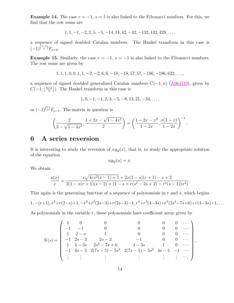
Example 14. The case r = −1, s = 1 is also linked to the Fibonacci numbers. For this, wefind that the row sums are

1, 1,−1,−2, 2, 5,−5,−14, 14, 42,−42,−132, 132, 429, . . . ,

a sequence of signed doubled Catalan numbers. The Hankel transform in this case is

(−1)(n+1

2 )Fn+2.

Example 15. Similarly, the case r = −1, s = −1 is also linked to the Fibonacci numbers.The row sums are given by

1, 1, 1, 0, 0, 1, 1,−2,−2, 6, 6,−18,−18, 57, 57,−186,−186, 622, . . . ,

a sequence of signed doubled generalized Catalan numbers C(−1; n) (A064310), given byC(−1; ⌊n+1

2⌋). The Hankel transform in this case is

1, 0,−1,−1, 2, 3,−5,−8, 13, 21,−34, . . . ,

or (−1)(n

2)Fn−1. The matrix in question is

(

2

3 −√

1 − 4x2,1 + 2x −

√1 − 4x2

2

)

=

(

1 − 2x − x2

1 − 2x,x(1 − x)

1 − 2x

)−1

.

6 A series reversion

It is interesting to study the reversion of xgQ(x), that is, to study the appropriate solutionof the equation

ugQ(u) = x.

We obtain

u(x)

x=

s√

4rx2(s − 1) + 1 + 2x(1 − s)(r + 1) − s + 2

2(1 − x(r + 1)(s − 2) + (1 − s + r(s2 − 2s + 2) − r2(s − 1))x2).

This again is the generating function of a sequence of polynomials in r and s, which begins

1,−(r+1), r2+r(2−s)+1,−r3+r2(2s−3)+r(2s−3)−1, r4+r3(4−3s)+r2(2s2−7s+6)+r(4−3s)+1, . . .

As polynomials in the variable r, these polynomials have coefficient array given by

N(s) =

1 0 0 0 0 0 · · ·−1 −1 0 0 0 0 · · ·1 2 − s 1 0 0 0 · · ·−1 2s − 3 2s − 3 −1 0 0 · · ·1 4 − 3s 2s2 − 7s + 6 4 − 3s 1 0 · · ·−1 4s − 5 2(7s − 5) − 5s2 2(7s − 5) − 5s2 4s − 5 −1 · · ·...

......

......

.... . .

,

14

which apart from signs, is also Pascal-like. Examples for s = 0, . . . , 5 of these matrices N(s)are given at the end of the last section. The central coefficients M(s)

1, 2 − s, 2s2 − 7s + 6,−5s3 + 24s2 − 38s + 20, 14s4 − 84s3 + 188s2 − 187s + 70, . . .

of this triangle are of interest. As polynomials in s, they can be expressed as

M(s) =n∑

k=0

(

2n

n − k

)

2k + 1

n + k + 1(−1)n−k(s−1)n−k =

n∑

k=0

(

2n − k − 1

n − k

)

k + 0n+k

n + 0nk(1−s)n−k(2−s)k.

The g.f. of M(s) is given by

gM(s) =1

1 + (s − 2)xc((1 − s)x)=

s − (s − 2)√

1 − (1 − s)4x

2(1 − (s − 2)2x).

They are the moments of the family of orthogonal polynomials Rn(x) defined by

Rn(x) = (x − 2(1 − s))Rn−1(x) − (s − 1)2Rn−2(x), n > 2,

with R0(x) = 1, R1(x) = x − (s − 2) and R2(x) = x2 + x(3s − 4) + (s − 1)(s − 2). Thecoefficient array of this family of polynomials is given by the Riordan array

(

1 − sx − (1 − s)x2

1 + 2(1 − s)x + (s − 1)2x2,

x

1 + 2(1 − s)x + (s − 1)2x2

)

.

The moments M(s) are then the elements of the first column of the inverse of this array.They can be represented as

Mn(s) =1

π

∫ 0

4(1−s)

xn (s − 2)√

x(4(1 − s) − x)

2x(x − s2 − 4(1 − s))dx

for s 6= 1, 2. The Hankel transform of Mn(s) is given by

hn(s) = (s − 2)n(s − 1)n2

.

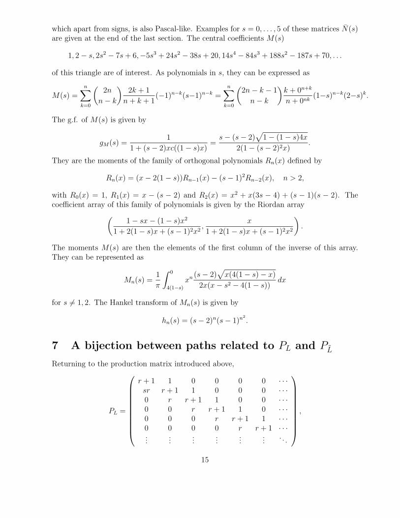
7 A bijection between paths related to PL and PL

Returning to the production matrix introduced above,

PL =

r + 1 1 0 0 0 0 · · ·sr r + 1 1 0 0 0 · · ·0 r r + 1 1 0 0 · · ·0 0 r r + 1 1 0 · · ·0 0 0 r r + 1 1 · · ·0 0 0 0 r r + 1 · · ·...

......

......

.... . .

,

15

we are now interested in these matrix entries and their corresponding Motzkin paths. It isknown [17, 22, 35] that the elements of the first column of the Riordan array correspondingto PL count Motzkin paths returning to the x axis. Motzkin paths related to the matrix PL

above are referred to as (r+1)-colored Motzkin paths, where we have a choice of (r+1) colorsfor each east step. Similarly, each south-east step has a choice of r colors. We note that forthe matrix above, the south-east step returning to the x axis has a choice of rs colors. Forthis reason, we will refer to such Motzkin weighted paths as (s-ex−axis, ex−axis; s-e, e)-Motzkinpaths. Thus, PL corresponds to a (rs, r+1; r, r+1)-Motzkin path. Similarly, it can be shown[22] that the first column of the Riordan array corresponding to the production matrix

PL =

r + 1 1 0 0 0 0 · · ·rs r 1 0 0 0 · · ·rs r r 1 0 0 · · ·rs r r r 1 0 · · ·rs r r r r 1 · · ·rs r r r r r · · ·...

......

......

.... . .

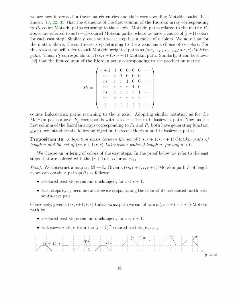
counts Lukasiewicz paths returning to the x axis. Adopting similar notation as for theMotzkin paths above, PL corresponds with a (rs, r + 1; r, r)- Lukasiewicz path. Now, as thefirst column of the Riordan arrays corresponding to PL and PL both have generating functiongQ(x), we introduce the following bijection between Motzkin and Lukasiewicz paths.

Proposition 16. A bijection exists between the set of (rs, r + 1; r, r + 1)-Motzkin paths oflength n and the set of (rs, r + 1; r, r)- Lukasiewicz paths of length n, for any n > 0.

We choose an ordering of colors of the east steps. In the proof below we refer to the eaststeps that are colored with the (r + 1)-th color as er+1

Proof. We construct a map φ : M → L. Given a (rs, r +1; r, r +1)-Motzkin path P of lengthn, we can obtain a path φ(P ) as follows:

• i-colored east steps remain unchanged, for i < r + 1.

• East steps er+1, become Lukasiewicz steps, taking the color of its associated north-east,south-east pair.

Conversely, given a (rs, r+1; r, r)- Lukasiewicz path we can obtain a (rs, r+1; r, r+1)-Motzkinpath by

• i-colored east steps remain unchanged, for i < r + 1.

• Lukasiewicz steps form the (r + 1)th colored east steps, er+1.

y axis

(r + 1)rsrs

r2s

(r + 1)rr

r2

16

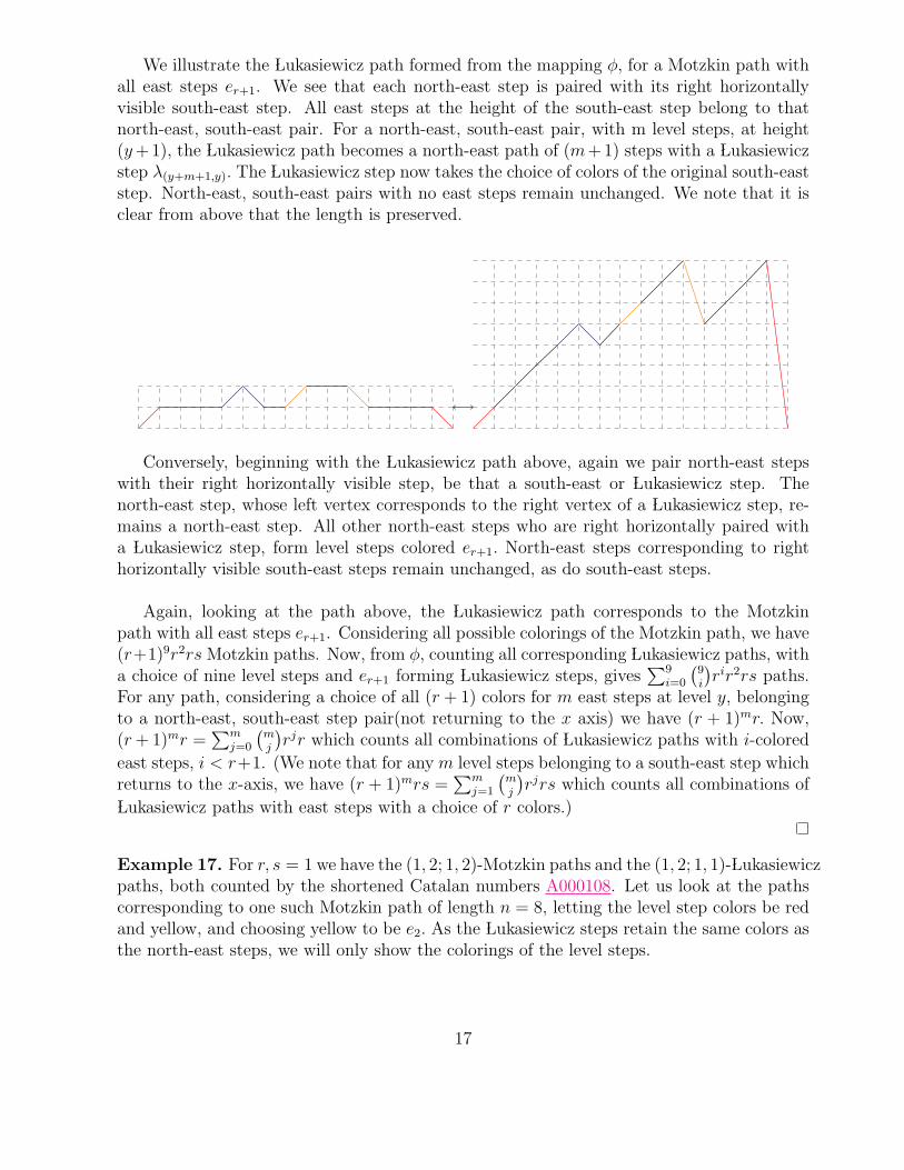
We illustrate the Lukasiewicz path formed from the mapping φ, for a Motzkin path withall east steps er+1. We see that each north-east step is paired with its right horizontallyvisible south-east step. All east steps at the height of the south-east step belong to thatnorth-east, south-east pair. For a north-east, south-east pair, with m level steps, at height(y + 1), the Lukasiewicz path becomes a north-east path of (m+ 1) steps with a Lukasiewiczstep λ(y+m+1,y). The Lukasiewicz step now takes the choice of colors of the original south-eaststep. North-east, south-east pairs with no east steps remain unchanged. We note that it isclear from above that the length is preserved.

Conversely, beginning with the Lukasiewicz path above, again we pair north-east stepswith their right horizontally visible step, be that a south-east or Lukasiewicz step. Thenorth-east step, whose left vertex corresponds to the right vertex of a Lukasiewicz step, re-mains a north-east step. All other north-east steps who are right horizontally paired witha Lukasiewicz step, form level steps colored er+1. North-east steps corresponding to righthorizontally visible south-east steps remain unchanged, as do south-east steps.

Again, looking at the path above, the Lukasiewicz path corresponds to the Motzkinpath with all east steps er+1. Considering all possible colorings of the Motzkin path, we have(r+1)9r2rs Motzkin paths. Now, from φ, counting all corresponding Lukasiewicz paths, witha choice of nine level steps and er+1 forming Lukasiewicz steps, gives

∑9i=0

(

9i

)

rir2rs paths.For any path, considering a choice of all (r + 1) colors for m east steps at level y, belongingto a north-east, south-east step pair(not returning to the x axis) we have (r + 1)mr. Now,(r + 1)mr =

∑m

j=0

(

m

j

)

rjr which counts all combinations of Lukasiewicz paths with i-colored

east steps, i < r+1. (We note that for any m level steps belonging to a south-east step whichreturns to the x-axis, we have (r + 1)mrs =

∑m

j=1

(

m

j

)

rjrs which counts all combinations of

Lukasiewicz paths with east steps with a choice of r colors.)

Example 17. For r, s = 1 we have the (1, 2; 1, 2)-Motzkin paths and the (1, 2; 1, 1)- Lukasiewiczpaths, both counted by the shortened Catalan numbers A000108. Let us look at the pathscorresponding to one such Motzkin path of length n = 8, letting the level step colors be redand yellow, and choosing yellow to be e2. As the Lukasiewicz steps retain the same colors asthe north-east steps, we will only show the colorings of the level steps.

17

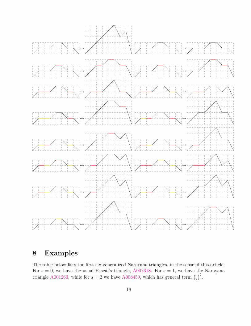
8 Examples

The table below lists the first six generalized Narayana triangles, in the sense of this article.For s = 0, we have the usual Pascal’s triangle, A007318. For s = 1, we have the Narayana

triangle A001263, while for s = 2 we have A008459, which has general term(

n

k

)2.

18

1 0 0 0 0 01 1 0 0 0 01 2 1 0 0 01 3 3 1 0 01 4 6 4 1 01 5 10 10 5 1

1 0 0 0 0 01 1 0 0 0 01 3 1 0 0 01 6 6 1 0 01 10 20 10 1 01 15 50 50 15 1

1 0 0 0 0 01 1 0 0 0 01 4 1 0 0 01 9 9 1 0 01 16 36 16 1 01 25 100 100 25 1

s = 0 s = 1 s = 21 0 0 0 0 01 1 0 0 0 01 5 1 0 0 01 12 12 1 0 01 22 54 22 1 01 35 160 160 35 1

1 0 0 0 0 01 1 0 0 0 01 6 1 0 0 01 15 15 1 0 01 28 74 28 1 01 45 230 230 45 1

1 0 0 0 0 01 1 0 0 0 01 7 1 0 0 01 18 18 1 0 01 34 96 34 1 01 55 310 310 55 1

s = 3 s = 4 s = 5

The next table lists some examples of the sequences Qn(r, s) for the values of r and s shown.

(r, s) Qn(r, s) OEIS number(0,1) 1, 1, 1, 1, 1, 1, . . . A000012(1,1) 1, 2, 5, 14, 42, 132, . . . A000108(n + 1)(2,1) 1, 3, 11, 45, 197, 903, . . . A001003(n + 1)(3,1) 1, 4, 19, 100, 562, 3304, . . . A007564(n + 1)(4,1) 1, 5, 29, 185, 1257, 8925, . . . A059231(n + 1)(0,2) 1, 1, 1, 1, 1, 1, . . . A000012(1,2) 1, 2, 6, 20, 70, 252, . . . A000984(2,2) 1, 3, 13, 63, 321, 1683, . . . A001850(3,2) 1, 4, 22, 136, 886, 5944, . . . A069835(4,2) 1, 5, 33, 245, 1921, 15525, . . . A084771(1,3) 1, 2, 7, 26, 100, 392, . . . A101850(1,4) 1, 2, 8, 32, 132, 552, . . . A155084

Finally, we document the start of the matrices N(s) for s = 0, . . . , 5.

19

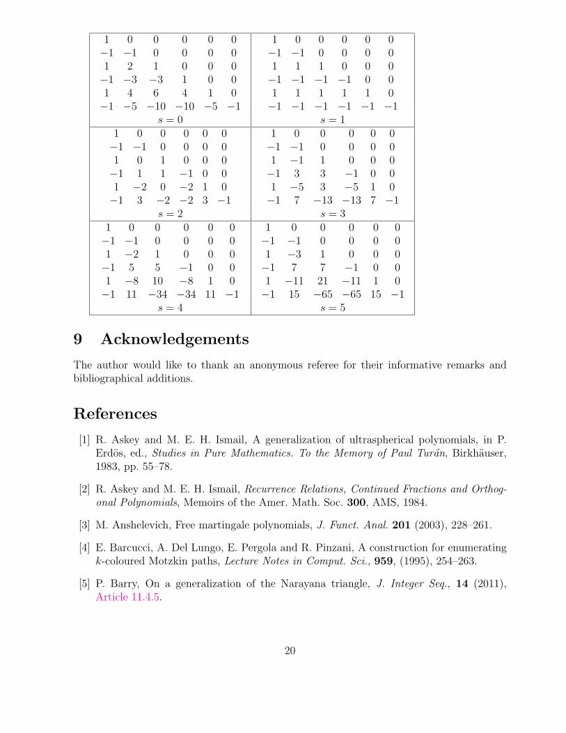
1 0 0 0 0 0−1 −1 0 0 0 01 2 1 0 0 0−1 −3 −3 1 0 01 4 6 4 1 0−1 −5 −10 −10 −5 −1

1 0 0 0 0 0−1 −1 0 0 0 01 1 1 0 0 0−1 −1 −1 −1 0 01 1 1 1 1 0−1 −1 −1 −1 −1 −1

s = 0 s = 11 0 0 0 0 0−1 −1 0 0 0 01 0 1 0 0 0−1 1 1 −1 0 01 −2 0 −2 1 0−1 3 −2 −2 3 −1

1 0 0 0 0 0−1 −1 0 0 0 01 −1 1 0 0 0−1 3 3 −1 0 01 −5 3 −5 1 0−1 7 −13 −13 7 −1

s = 2 s = 31 0 0 0 0 0−1 −1 0 0 0 01 −2 1 0 0 0−1 5 5 −1 0 01 −8 10 −8 1 0−1 11 −34 −34 11 −1

1 0 0 0 0 0−1 −1 0 0 0 01 −3 1 0 0 0−1 7 7 −1 0 01 −11 21 −11 1 0−1 15 −65 −65 15 −1

s = 4 s = 5

9 Acknowledgements

The author would like to thank an anonymous referee for their informative remarks andbibliographical additions.

References

[1] R. Askey and M. E. H. Ismail, A generalization of ultraspherical polynomials, in P.Erdos, ed., Studies in Pure Mathematics. To the Memory of Paul Turan, Birkhauser,1983, pp. 55–78.

[2] R. Askey and M. E. H. Ismail, Recurrence Relations, Continued Fractions and Orthog-onal Polynomials, Memoirs of the Amer. Math. Soc. 300, AMS, 1984.

[3] M. Anshelevich, Free martingale polynomials, J. Funct. Anal. 201 (2003), 228–261.

[4] E. Barcucci, A. Del Lungo, E. Pergola and R. Pinzani, A construction for enumeratingk-coloured Motzkin paths, Lecture Notes in Comput. Sci., 959, (1995), 254–263.

[5] P. Barry, On a generalization of the Narayana triangle, J. Integer Seq., 14 (2011),Article 11.4.5.

20

[6] P. Barry and A. Hennessy, A note on Narayana triangles and related polynomials, Rior-dan arrays and MIMO capacity calculations, J. Integer Seq., 14 (2011), Article 11.3.8.

[7] P. Barry, Riordan arrays, orthogonal polynomials as moments, and Hankel transforms,J. Integer Seq., 14 (2011), Article 11.2.2.

[8] P. Barry and A. Hennessy,Meixner-type results for Riordan arrays and associated integer sequences, J. IntegerSeq., 13 (2010), Article 10.9.4.

[9] P. Barry, Continued fractions and transformations of integer sequence, J. Integer Seq.,12 (2010), Article 09.7.6.

[10] P. Barry, A Catalan transform and related transformations on integer sequences, J. ofInteger Seq., 8 (2005), Article 05.4.5.

[11] M. Bozejko and W. Bryc, On a class of free Levy laws related to a regression problem,J. Funct. Anal. 236 (2006), 59–77.

[12] G-S. Cheon, H. Kim, and L. W. Shapiro, Riordan group involutions, Linear AlgebraAppl., 428 (2008), 941–952.

[13] J. M. Cohen and A. R. Trenholme, Orthogonal polynomials with constant recursionformula and an application to harmonic analysis, J. Funct. Anal. 59 (1984), 175–184.

[14] B. Collins, Product of random projections, Jacobi ensembles and universality problemsarising from free probability, Probab. Theory Related Fields 133 (2005), 315–344.

[15] E. Deutsch, L. Ferrari, and S. Rinaldi, Production matrices, Adv. in Appl. Math. 34

(2005), 101–122.

[16] E. Deutsch, L. Ferrari, and S. Rinaldi, Production matrices and Riordan arrays, Ann.Comb., 13 (2009), 65–85.

[17] P. Flajolet, Combinatorial aspects of continued fractions, Discrete Math., 32 (1980),125–161.

[18] J. Geronimus, On a set of polynomials, Ann. of Math. 31 (1930), 681–686.

[19] I. Graham, D. E. Knuth, and O. Patashnik, Concrete Mathematics, Addison–Wesley,1995.

[20] F. A. Grunbaum, Random walks and orthogonal polynomials: some challenges, in M.Pinsky, B. Birner, eds., Probability, Geometry and Integrable Systems MSRI publications55 CUP 2008, 241–260.

[21] Tian-Xiao He, R. Sprugnoli, Sequence characterization of Riordan arrays, DiscreteMath. 2009 (2009), 3962–3974.

21

[22] A. Hennessy, A study of Riordan arrays with applications to continued fractions, or-thogonal polynomials and lattice paths, PhD Thesis, Waterford Institute of Technology,2011.

[23] S. Karlin and J. L. McGregor, The differential equations of birth-and-death processes,and the Stieltjes moment problem, Trans. Amer. Math. Soc. 85 (1957), 489–546.

[24] C. Krattenthaler, Advanced determinant calculus, Seminaire Lotharingien Combin. 42

(1999), Article B42q., available electronically athttp://arxiv.org/abs/math/9902004, 2012.

[25] C. Krattenthaler, Advanced determinant calculus: a complement, Linear Algebra Appl.411 (2005), 68–166.

[26] J. W. Layman, The Hankel transform and some of its properties, J. Integer Seq. 4

(2001), Article 01.1.5.

[27] Franz Lehner, Cumulants, lattice paths and orthogonal polynomials,Discrete Math.,270 (2003), 177–191.

[28] V. A. Marcenko and L. A. Pastur, Distribution of eigenvalues in certain sets of randommatrices, Math. USSR Sb. 1 (1967), 457–483.

[29] N. Saitoh and H. Yoshida, The infinite divisibility and orthogonal polynomials with aconstant recursion formula in free probability theory, Probab. Math. Statist. 21 (2001),159–170.

[30] L. W. Shapiro, S. Getu, W.-J. Woan, and L.C. Woodson, The Riordan Group, Discr.Appl. Math. 34 (1991), 229–239.

[31] N. J. A. Sloane, The On-Line Encyclopedia of Integer Sequences. Published electroni-cally at http://oeis.org, 2012.

[32] N. J. A. Sloane, The On-Line Encyclopedia of Integer Sequences, Notices Amer. Math.Soc., 50 (2003), 912–915.

[33] R. Sprugnoli, Riordan arrays and combinatorial sums, Discrete Math. 132 (1994), 267–290.

[34] G. Szego, Orthogonal Polynomials, 4th ed., American Mathematical Society, 1975.

[35] X. Viennot, Une theorie combinatoire des polynomes orthogonaux generaux, lecturenotes, UQAM, 1983.

2010 Mathematics Subject Classification: Primary 11B83; Secondary 15B36, 42C05, 11C20,15B05.

22

Keywords: Narayana polynomial, Riordan array, production matrix, orthogonal polynomial,Hankel transform.

(Concerned with sequences A000007, A000012, A000045, A000108, A000169, A000984, A001003,A001263, A001850, A006125, A007318, A007564, A008459, A059231, A064062, A064310,A069835, A083667, A084771, A099169, A101850, A143464, A155084, A187021.)

Received November 9 2011; revised version received April 17 2012. Published in Journal ofInteger Sequences, April 20 2012.

Return to Journal of Integer Sequences home page.

23