Embed Size (px)
Citation preview

SOLVING THE RUBIK’S CUBE WITH PARALLEL PROCESSING
By
ASLESHA NARGOLKAR
Presented to the Faculty of the Graduate School of
The University of Texas at Arlington in Partial Fulfillment
Of the Requirements
For the Degree of
MASTER OF SCIENCE IN COMPUTER SCIENCE ENGINEERING
THE UNIVERSITY OF TEXAS AT ARLINGTON
May 2006

Copyright © by Aslesha Nargolkar 2006
All Rights Reserved

iii
ACKNOWLEDGEMENTS
I would like to express my sincere thanks to my Dr. Ishfaq Ahmad for his
continuous support, guidance and encouragement through out the course of my
research. It was because of him that I was able to do research on this topic and complete
my thesis. I would also like to thank Patrick Mcguian for all his help in running the
experiments on the DPCC cluster.
I also owe my thanks to my mother, father, brother and my family for their
support and encouragement. The same is true for all my friends who remained behind
me and encouraged me throughout my Masters study.
November 21, 2005

iv
ABSTRACT
PARALLEL PROCESSING A RUBIK’S CUBE
Aslesha Nargolkar, M.S.
The University of Texas at Arlington, 2006
Supervising Professor: Dr. Ishfaq Ahmad
This thesis investigates parallel processing techniques for solving the 3 x 3 x 3
Rubik’s Cube. We explore various state-space search based algorithmic approaches to
optimally solve the Cube. The parallel processing approach is based on IDA* using a
pattern database as the underlying heuristic because of its well established effectiveness.
The parallel algorithm is an extension of the Michael Reid algorithm which is sequential.
The parallel algorithm exhibits good speedup and scalability. Nearly 150 random as well
as symmetrical cube configurations were tested for the experiments on sequential and
parallel implementations. The proposed parallel algorithm using master-slave type of
load balancing proves efficient in terms of time as well as memory resources while
yielding an optimal solution to find the state of a Rubik’s cube. Parallel processing helps
in solving a Cube with initial cube configurations having solutions at a higher depth level

v
in the search tree. Various comparative results are provided to support the efficiency of
the parallel implementation.

vi
TABLE OF CONTENTS
ACKNOWLEDGEMENTS ……………………………………………………… iii
ABSTRACT…………………………………………………………………......... iv
LIST OF ILLUSTRATIONS..................................................................................... ix
LIST OF TABLES..................................................................................................... x
Chapter
1. INTRODUCTION…………. ........................................................................ 1
1.1 The 3x3x3 Cube………………............................................................... 1
1.1.1 Different pieces of the Cube…………………......................... 3
1.1.2 Singmaster notation…………………………………………... 3
1.1.3 The Metrics…………………. ................................................. 4
1.1.4 The Super flip position............................................................. 5
1.1.5 Solving the Cube……………….............................................. 5
1.2 Background…..…………….................................................................... 6
1.3 Organization of the thesis……. ............................................................... 7
2. STANDARD ALGORITHMS…… .............................................................. 8
2.1 God’s algorithm……………................................................................... 8
2.2 Basic tree searches……........................................................................... 8
2.2.1 Uninformed searches……….................................................... 9
2.2.2 Informed searches……….…………………............................ 9
2.2.2.1 Greedy Best-First Search ……………………………. 10

vii
2.2.2.2 Uniform cost…………………………………………. 10
2.2.2.3 A*……………………………………………………. 11
2.3 Iterative Deepening A*………………………………………………...… 11
2.3.1 Standard IDA*……..……. .......................................................... 12
2.3.2 Problem with this approach…… ................................................. 12
2.3.3 Solution: IDA* with pattern databases…………………………. 14
2.4 Thistlehwaite’s algorithm ……………………………………………….. 15
2.5 Kociemba’s algorithm…………………………. ....................................... 16
2.6 Korf’s algorithm……………………………. ............................................ 16
2.7 Reid’s algorithm……………………………. ............................................ 17
3. PARALLEL PROCESSING ……………………………………………………. 19
3.1 Algorithm………………………………………………....………………. 19
3.2 Performance metrics ………………………………....………………….. 20
3.2.1 Execution time ……. ................................................................... 21
3.2.2 Efficiency……..……................................................................... 22 3.2.3 Speedup……………..…….......................................................... 22
3.2.4 Serial Fraction….......................................................................... 22
3.3 Performance evaluation of a parallel algorithm………………………… 23
4. IMPLEMENTATION………................................................................................ 24
4.1 Use of symmetry……………….............................................................. 25
4.2 Creation of pattern database….. .............................................................. 26
4.3 Pseudo code for the parallel implementation …………………………… 26

viii
5. EXPERIMENTAL METHODOLOGY................................................................ 28
5.1 Results Analysis…………………………………………………………. 28
5.1.1 Results for the sequential implementation …………………... 29
5.1.2 Results for the parallel implementation …………………........ 32
5.1.3 Comparisons …………………………………………………... 33
5.1.4 Comparisons of results for the super flip configuration …….. 35
6. CONCLUSIONS……………………………………………………………….. 37
APPENDIX
A. SEARCH TREE SIMULATION…..………………………………………. 39
B. PROGRAM EXECUTION MODULE …………………………………….. 43
C. PATTERNS USED IN EXPERIMENTATION…………………………… 47
D. PROFILING OUTPUT …………………………………………………….. 50
REFERENCES…...……………………………………………………………….. 52
BIOGRAPHICAL INFORMATION ……………………………………………… 55

ix
LIST OF ILLUSTRATIONS
Figure Page
1.1 The Rubik’s Cube……………………………………………………………. 2
2.1 Number of nodes generated Vs Depth….. ........................................................ 13
2.2 Execution time Vs Depth……………………. ............................................... 14
4.1 Data Flow Diagram …………………………………………………………. 27
5.1 Average Time Vs Depth (12-18) for Reid’s sequential implementation …… 29
5.2 Average Time Vs Depth (19-22) for Reid’s sequential implementation……. 30
5.3 Average Time Vs Depth for Reid’s sequential algorithm……………………. 31
5.4 Average Time Vs Depth for the parallel implementation with np=8…........... 32
5.5 Comparisons of time in minutes required to solve the cube for 8 random cubes of depth 21 ………………………………………………….. 34
5.6 Comparisons of time in minutes required to solve the inverse for 8 random cubes of depth 21…………………………………………………… 35
5.7 Time in hours required to solve the super flip position Vs Number of processors used ………………………………………………………....... 36

x
LIST OF TABLES
Table Page
2.1 Moves per stage in the Thistlethwaite’s algorithm …………………………… 16
5.1 Data for average time Vs depth (12-18) for Reid’s sequential implementation……………………………………………………………….. 30
5.2 Data for average time Vs depth (19-22) for Reid’s sequential implementation ………………………………………………………………. 31
5.3 Data for average time Vs depth for the parallel implementation using np=8… 32
5.4 Data for Time in hours Vs Number of processors required to solve the Super Flip position ……………………………………………….………….. 36

1
CHAPTER 1
INTRODUCTION
Improving an algorithm to solve a Rubik’s cube requires a thorough analysis of
past efforts in both multi-processor algorithms and sequential solutions to the problem.
With the extensive experimentation carried out, it became clear that Manhattan distance
heuristic, as was used in our first approach, was not the best approach. During the
course of the research work and the experimentation done, it became clear that pattern
databases as modified by Michael Reid [26] is perhaps the best existing heuristic for
this problem. The use of pruning and symmetry improve the pattern database and hence
the performance of the algorithm. Also, parallelization of the search would maximize
the success of the algorithm being used while reducing the time required in finding a
solution for larger depths (above 18). Hence all the necessary issues related to the
parallel approach like the load balancing techniques and the task distribution and
scalability would need to be considered. Although the heuristic used is improved, the
algorithm used for searching remains the same, IDA*. The experiments carried out
show the number of nodes generated and the time taken for the most difficult known
configuration: the super flip configuration. This is a 24-depth configuration.
1.1 The 3x3x 3 Cube
Rubik’s cube is considered to be one of the most famous combinatorial puzzles
of its time. Erno Rubik of Hungary invented it in the late 1970s. The standard version of

2
this cube consists of a 3 X 3 X 3 cube (Figure 1.1), with a different color on each face:
red, blue, green, yellow, white and orange. The faces are divided into 9 squares each,
which can be scrambled by rotating a row (or column) at a time. It is divided into three
3×3×1 slices along each of x, y, and z axes such that each slice can be rotated a quarter
turn clockwise or counterclockwise with respect to the rest of the cube. The slices
divide each face of the Cube into 9 facelets. The slices also divide the Cube into 33 = 27
pieces, or sub cubes, 26 of which are visible. In its goal state, each of the six sides has
its own color. Each visible piece has one, two or three facelets that are a unique subset
of the colors, which makes it distinct from the others. This preserves the orientation of
the piece as it changes position as the slices are rotated.
Figure 1.1: The Rubik’s Cube (Note the numbers in bracket denote the number of those pieces in a 3x3 Cube)
Edge Cubelet (12)
Cubelet (27)
Facelet (54)
Corner Cubelet (8)

3
1.1.1 Different pieces of the Cube
Of the 27 sub cubes, or cubies, 26 are visible, and of those only 20, the 8 corner
pieces with three facelets and the 12 edge pieces with two facelets, actually move. The
corner pieces only move to other corner positions, or cubicles, and edge pieces only
move to other edge cubicles. The center pieces with a single facelet in the center of
each face merely rotate. The corner pieces can be twisted any of three ways. Likewise,
the edge pieces can be flipped either of two ways. Thus, the corner pieces have three
orientations each, and the edge pieces have two orientations each.
1.1.2 Singmaster notation
Singmaster notation devised by David Singmaster [2] describes a sequence of
moves. Clockwise turns of the six outer layers, or slices, are denoted by the capital
letters where F is front, B is back, U is up, D is down, L is left and the right face is
denoted by an R:
<F, B, U, D, L, R> which are 90 degrees clockwise face moves
<F2, B2, U2, D2, L2, R2> which are 180 degrees clockwise face moves
<F’, B’, U’, D’, L’, R’>which are 270 degrees clockwise i.e. 90 degrees
anticlockwise face moves
If a subsequence of moves is repeated then it is listed in parenthesis with an
exponent equal to the number of repetitions. Singmaster notation is also used to label
each of the cubies and cubicles. Lowercase italicized letters given in clockwise order of

4
how the two or three sides intersect at a given corner or edge are used to describe a
cubie. Uppercase is used to denote cubicles. Since there are either two or three
possibilities depending on which side is listed first, the first letter is given in order of U,
D, F, B, R, L. While the cubicles never change orientation, the cubies do. So this
precedence in labeling cubies is with respect to the goal state. Thus URF and not RFU
would be used to denote the upper front right-hand cubicle. The cubie corresponding to
that cubicle would be denoted by urf if its orientation has not changed from the goal
state and as either rfu or fur if it had. The orientation is determined by keeping track of
how the pieces move from cubicle to cubicle with respect to the initial state. If an R
move was applied to the goal state, then u facelet of the urf cubie would move to the b
facelet of the UBR cubicle. Thus, with u b, r r, and f u, the corner piece would
then become fur.
1.1.3 The Metrics
To reach the goal state from any random configuration, a sequence of moves is
applied. The minimum number of these moves required to solve the Cube is known as
the distance from the goal state while the maximum distance is the diameter of the
Cube. These moves or distances are measured using either the Half Turn Metric (HTM)
or the Quarter Turn Metric (QTM). In the first metric, only half turns are allowed while
in the quarter turn metric, only quarter turns are allowed. Such a sequence of moves
used to get to the goal state is known as a macro operator or a macro.
The Cube can be represented by a graph in which a vertex represents a unique
state and an edge represents a transition between adjacent states. Since there are 18

5
elementary moves, there are 18 possible adjacent states. The branching factor is
considered to be the ratio of the number of nodes explored at a given depth (d+1) over
the number of nodes explored at a depth d.
1.1.4 The Super flip position
Cube solving has been proven to generally take less than 20 moves. But the
diameter of the cube is said to be the super flip position which is known to take 24
moves. [26] It is not maximally distant from the start position. It is also known as 12-
flip, all-flip, all-edges-flipped.
1.1.5 Solving the Cube
This puzzle is challenging to solve because of the large number of different
states that can be reached from any configuration. The goal state in this puzzle is the
state with all the squares on each side of the cube having the same color. In addition,
large memory requirements and computational resources are required to solve this
problem, which is also the reason why it has been labeled as a very difficult problem.
Although several algorithms have been successfully developed to solve the Rubik’s
cube on sequential machines, they all face the same problem of limited memory and
computational requirements, especially when trying to find an optimal solution and
when we consider the required amount of time for those algorithms to find a solution.
Therefore, parallelizing the algorithm seems to be promising in terms of reducing
execution time and having enough resources to find a solution.
The Rubik’s cube has also been an interesting research problem in the Artificial
Intelligence area. Researchers had reached a consensus that an informed searching

6
methodology is the most feasible way to find a solution in such a vast search space. The
fact that finding a solution to this puzzle will require a large memory and better
computational resources has made it difficult to run efficiently on sequential machines,
thus parallelizing the search is the next best choice along with reducing the
computational complexity. It is however true that we need to ensure that we make the
best of the scalability and all other available resources of the parallel hardware. Since
each cube configuration leads to a large number of states, the search space unfolds in
the shape of a tree, so parallelizing can be done by handing over the branches of the tree
to separate processors for performing search independently. One such architecture that
could fulfill all our requirements regarding memory and power resources is the cluster
of workstations.
1.2 Background
A standard 3 X 3 X 3 Rubik’s cube can have 4.3252 X 10¹⁹ different states from
a given configuration. In our initial approach, to reduce large computational complexity
involved in finding a solution to this puzzle, we had used a two dimensional flat
representation obtained by opening the cube along its edges. This representation can
then be converted into an array representation with each color being represented by a
numerical value.
The search algorithm used was the Iterative Deepening A* (IDA*) algorithm
which is an optimal, memory bounded heuristic search. A heuristic function provides an
estimate of the distance of a particular state from a goal state. The heuristic used was
the one Richard Korf (1997) [1, 5] had suggested. It was a modified version of the

7
Manhattan heuristic used in the sliding puzzle where the Manhattan distance of only the
edge cubes was calculated.
The performance of the search can be improved by using parallel hardware. But
the choice of heuristic is another main factor affecting the performance of the algorithm.
Heuristics functions should be chosen properly to avoid inherent problems pertaining to
high time complexity. If there is no overestimation of depth then the proposed method
is guaranteed to improve the performance of IDA* algorithm.
1.3 Organization of the thesis
The rest of the thesis is organized into different chapters, starting with Chapter 2
where all the standard optimal algorithms are explained. This same chapter also
explains the standard IDA* algorithm along with the IDA* algorithm used with pattern
databases. The actual method of implementation with the experiment results is given in
Chapters 3, 4, 5. The thesis is concluded with Chapter 6.

8
CHAPTER 2
STANDARD ALGORITHMS
Michael Reid’s optimal cube solver [26] is based on ideas developed by Herbert
Kociemba [24] and Professor Richard Korf [5]. This is supposed to be a practical
implementation of "God's Algorithm" [7] for Rubik's Cube. He has made some
improvements in the Korf’s method.
2.1 God’s Algorithm
God’s algorithm [7] uses a lookup table that is keyed over the various instances
of the problem. Rather than giving the solution, it gives the minimum number of moves
remaining to reach the goal state. Then to solve a particular instance one simply
chooses the next move that is one closer to the goal state. The lookup table can be
further refined to only store the number of moves left modulo 3, which only requires 2
bits per entry. This is sufficient in picking the next move since any adjacent move is
one less, the same or one more towards the solution.
2.2 Basic tree searches
This can be thought of as tree in which the root node is the initial state, and
each level below is the nodes explored at that given depth. The nodes in the tree need
not be unique. Pruning techniques can be used to reduce the likelihood of encountering
duplicates.

9
2.2.1 Uniformed searches
Given the extreme number of state, 4.3 1019, uninformed searches such as BFS
(breadth first search) or DFS (depth first search) turn out to be impractical. While BFS
a slow and methodical search that is guaranteed to produce an optimal solution, it
doesn’t work since all the states must be kept in memory, which clearly exceeds the
memory limit of on any conventional computer.
DFS fails for several reasons. First of all, there is no guarantee it won’t run into
some infinite cycle. To correct this one can limit the depth to which it explores.
However, then there is no guarantee it will find the goal state. To further correct the
problem, one can employ an incremental DFS, in which one incrementally increases the
depth being explored. But the advantage of DFS over BFS is that it can potentially find
the solution quite quickly if it happens to select nodes that lead to the solution. It also
has the advantage of only having a linear memory complexity that is ( )O b d where b is
the asymptotic branching factor and d in this case is the depth of the search. The
disadvantage of DFS used without iterative deepening is that it is not optimal in that
there is no guarantee it will choose the shortest path, nor is it complete in that there is
no guarantee it will explore the whole graph.
2.2.2 Informed Searches
Informed searches like best-first search keeps a queue of the nodes left to
explore and orders them by some evaluation function that attempts to select the best
10
nodes to search first. Two versions of best-first search base the evaluation function
either on the distance incurred or estimated distance remaining.
2.2.2.1 Greedy Best-First Search
Greedy best-first search orders the nodes in the queue based on an estimate of
the distance remaining to the goal state. As the greedy estimate becomes accurate, this
algorithm becomes more similar to God’s algorithm. To increase the likelihood of the
solution found to be optimal, it helps if the estimate never overestimates the distance
remaining. Such an estimate is known as an admissible heuristic. This increases the
chances that the shortest path will be found.
Greedy search is also a way of directing a standard DFS search. It chooses the
next node to explore based on some greedy estimate of the distance remaining to the
goal state. However, this approach cannot be used in conjunction with iterative
deepening since that would force the tree to be explored up to a given depth. As such it
suffers from the same limitations of DFS in that it is neither optimal nor complete.
However, it is more likely to find the solution before iterative deepening DFS.
2.2.2.2 Uniform cost
Uniform cost best-first search, known more simply as uniform cost, orders the
elements in the queue by the distance from the initial state. Here the distance for the
Rubik’s Cube is simply based on the number moves from the initial state, which makes
this uniform cost equivalent to BFS. However, if one were to favor some moves over
others and weight them accordingly, then uniform cost would still produce an optimal
solution, i.e. a path to the goal with minimum weight.

11
2.2.2.3 A*
A* combines the two best-first searches of uniform cost with the greedy search
using an admissible heuristic to produce an optimal search that is more efficient than
standard BFS, by setting its heuristic to be the sum of the distance from the initial state
and is admissible estimate of the distance to the goal state. The basic idea behind the
proof of optimality is that by keeping track of distance one has come in addition to how
far one has to go; one will never choose a path longer than necessary.
2.3 Iterative Deepening A*
Iterative-Deepening A*, also known as IDA*, was introduced by Richard Korf
in 1985 [4]. It has since become the dominate method to solve this class of permutation
puzzles to which Rubik’s Cube belongs. Where A* fails, IDA* tends to succeed given
strong enough admissible heuristic.
2.3.1 Standard IDA*
IDA* is simply A* with iterative deepening. This reduces the memory
complexity from ( )dO b to ( )O b d . It does this by keeping track of the maximum depth
explored from the last iteration and incrementally increases it. By doing so, it no longer
needs to store all the states in memory. The optimality of A* still applies, so IDA* also
gives an optimal solution. The Manhattan distance is less useful as a heuristic for the
Cube since if one were to total the number of moves necessary to place each cubie, one

12
must divide that total by eight since eight cubies are moved for each rotation of a slice
of the Cube. This results in a very low heuristic value.
2.3.2 Problem with this approach
Although IDA* is the best fit to solve the Rubik’s cube, as it was previously
discussed in this paper, the search space size remains one of the main problems to solve
in order to obtain an optimal solution. Therefore, we need to optimize IDA*, by
reducing the search space.
Initially the algorithm was tested for obtaining solutions up to depths 12. But
Korf mentions in his paper “Finding optimal solutions to Rubik’s Cube using pattern
databases” [5], that at depth over 15 are real significant moves and that any problem can
generally be solved in nearly 18 moves. For the same purpose of experimentation of his
approach, he had generated ten solvable instances of Rubik’s Cube, one solvable in 16
moves, three 17 and six requiring 18 moves. For all further studies related to the
Rubik’s Cube solution these 10 instances were used as standard. We also carried out
experiments on our sequential program [6] with these input configurations to get the
time required and the number of nodes generated. These programs were run in the
cluster of workstations at UTA, where every job submitted is assigned a dedicated
processor.
All programs were running for more than 50 hours of processing at depth 14
itself. The programs were writing output every 20 minutes, indicating what depth they
are working on, and the number of the iteration they are in, making sure they were not
stuck in an infinite loop. The program was also modified to reduce the amount of

13
memory needed to store every node and therefore decreasing the possibility of memory
problems. The program was extensively tested with depths up to 13, and the program
reported the optimal solutions for each configuration of the cube that was tested.
However, the results show that the technique used in the program may not be the most
effective. The same is illustrated in the following charts:
NODES GENERATED BY DEPTHS 7 TO 14 FOR EACH CUBE
0
200000000
400000000
600000000
800000000
1000000000
1200000000
7 8 9 10 11 12 13 14
DEPTH
NO
DE
S
Cube # 1
Cube # 2
Cube # 3
Cube # 4
Cube # 5
Cube # 6
Cube # 7
Cube # 8
Cube # 9
Cube # 10
Figure 2.1: Number of nodes generated Vs Depth
14
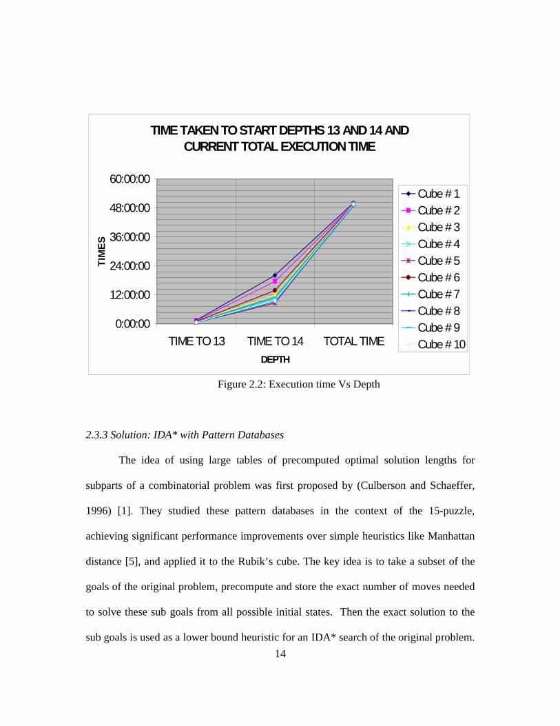
TIME TAKEN TO START DEPTHS 13 AND 14 AND CURRENT TOTAL EXECUTION TIME
0:00:00
12:00:00
24:00:00
36:00:00
48:00:00
60:00:00
TIME TO 13 TIME TO 14 TOTAL TIME
DEPTH
TIM
ES
Cube # 1Cube # 2Cube # 3
Cube # 4Cube # 5Cube # 6Cube # 7Cube # 8Cube # 9Cube # 10
Figure 2.2: Execution time Vs Depth
2.3.3 Solution: IDA* with Pattern Databases
The idea of using large tables of precomputed optimal solution lengths for
subparts of a combinatorial problem was first proposed by (Culberson and Schaeffer,
1996) [1]. They studied these pattern databases in the context of the 15-puzzle,
achieving significant performance improvements over simple heuristics like Manhattan
distance [5], and applied it to the Rubik’s cube. The key idea is to take a subset of the
goals of the original problem, precompute and store the exact number of moves needed
to solve these sub goals from all possible initial states. Then the exact solution to the
sub goals is used as a lower bound heuristic for an IDA* search of the original problem.

15
The idea behind the pattern database was to avoid the runtime computation of the
heuristic, at the expense of the extra memory storage. Since we have a large
computational engine in the form of a cluster we don’t need to worry about the extra
runtime computation.
2.4 Thistlethwaite’s algorithm
By restricting the type of moves used, different subgroups could be formed. If
only half moves were allowed then the subgroup will be <L2, R2, F2, B2, U2, D2>.
There could be some more nested subgroups in this, like <L2, R2, F, B, U, D> formed
by applying half turns only to the right and the left faces so that no edges can be flipped
or disoriented. These subgroups help since they have a comparatively smaller order.
Similarly, the corner orientations can be further fixed by restricting the half turns for the
front and the back by the subgroup <L2, R2, F2, B2, U, D>. The goal state or the
identity can be seen as a subgroup of these successively nested subgroups.
In the early 1980’s, the English mathematician Morwen B. Thistlethwaite
devised an algorithm [7] with the use of these nested subgroups in a lookup table. His
solution progressed from one nested subgroup to the other until the goal state. There
were tables for every stage and at every stage to move from one subgroup to the next;
the properties of the subgroup leading to the factors composing the two nested
subgroups were used for indexing in the tables. This algorithm gave the first known
diameter of the Cube as 52. With further improvements, he had improved the best
known upper bound to 45.

16
Table 2.1 – Moves per stage in the Thistlethwaite’s algorithm
Stage: 1 2 3 4 Total
Original algorithm: 7 13 15 17 52
Improved algorithm: 7 13 15 15 50
Best possible: 7 10 13 15 45
2.5 Kociemba’s algorithm
Herbert Kociemba of Germany [24] developed an algorithm that to date is the
algorithm that produces the best near optimal solutions in the shortest amount of time.
It typically runs in a few minutes whereas finding an optimal for the same state may
take far longer. Kociemba came upon the idea of only using <L2 R2, F2, B2, U, D> as
an intermediate nested subgroup. Using IDA* with this sub group for his pattern
database instead of lookup tables, he then searched for a position in it. By keeping track
of the maneuvers to get there and subsequently using IDA* again to search from that
position in the sub group to the goal state, he obtained a near optimal solution by
combining the two sets of maneuvers.
2.6 Korf’s algorithm
In his 1997 paper [5], Korf used the eight corners as one sub problem and two
sets of six of the twelve edges for the two others, which completely covers the Cube in

17
that any of the 20 movable pieces is in one of these three sets. For his heuristic he
examined the eight or six cubies in one of these smaller problems (smaller in the sense
of far fewer states) and looked up the remaining number of moves to solve that sub
problem. To create an admissible heuristic, he took the maximum of the three.
Michael Reid [26] improved this approach first suggested by Korf using the
pattern database to find optimal solutions for the Rubik’s Cube. This particular pattern
database produced a better heuristic than the ones based off of corners and edges used
by Korf. In fact IDA* ran twenty times faster for Reid on a slower computer using less
memory. The main concept here is that pattern databases need not be based off subset
of puzzle pieces, but more generally, can be based off any subgroup of the appropriate
order.
2.7 Reid’s algorithm
Michael Reid [26] uses distances to the intermediate position: <U, D, F2, R2,
B2, L2> for the pattern database. If there is a group G and a subgroup H, then for each
element g from G the set {a*g | a belongs to H} is called a right coset of H. Each
scrambled cube can be seen as a permutation with attached orientations. Coordinates
represent cosets; each coset usually consists of many permutations. Equivalent cubes
have the same structure but the number of moves necessary to solve them is the same.
Equivalence is defined with permutations. For each cube there are up to 48 equivalent
cubes, because the cube has 48 symmetries including reflections. Every closet in the
subgroups is characterized by corner orientation, edge orientation, location of the four
U-D slice edges. Since this gives a lot of configurations, symmetry is used. Also, 2

18
coordinates edge and location are combined into a single coordinate and it is divided by
the 16 symmetries. A BFS is done in the coset-space to calculate the distances to be
stored.

19
CHAPTER 3
PARALLEL PROCESSING
3.1 Algorithm
The parallel implementation aims to save time as well as memory resources
while doing the extensive search to the goal state. In the parallel implementation, every
processor searches separately to get a solution to the cube. Since every processor will
need a copy of the pattern databases and to avoid communication to pass this whole
structure to every processor, the initialization part of these databases is done by every
processor. The communication is further lessened with every processor having its own
copy of the cube configuration and initial variables to begin the processing. In this
parallel implementation, every processor searches the same tree but the iterative
deepening A* algorithm runs on every processor with different search limits. The work
distribution is done using a master-slave technique where every processor
communicates with the master, or processor 0, for the current search limit that it has to
search with. This assures that no processor is left without any work. Though processor 0
has to communicate with all the remaining processors, it does take part in computation
too.
The algorithm terminates when goal state is found by one of the
processors with an optimal path. When a processor searching along a particular branch

20
of the tree comes across the goal node, it sends the goal found information first to
processor 0 and then to the others. This goal found declaration is done in an
asynchronous manner. Before beginning the search, every processing element waits for
the goal found declaration using an asynchronous receive. Once the node is found an
exit message is sent to all the processors by the processor which finds the goal using a
non-blocking send call. Upon the receipt of the goal found declaration every processor
exits the communication world if the goal found is optimal and the processor which
found the goal prints the goal along with the steps to reach the goal before exiting the
communication world itself.
The different search limits help in finding the solution to the configuration faster
than the serial implementation because an increase in the search limit means more
pattern subgroup matches from the pruning tables or pattern databases. And these could
mean a faster and shorter search at most of the times. Another factor that aids in faster
search is the symmetry, a symmetrical configuration is observed to be running faster
than an asymmetrical one.
3.2 Performance metrics
The behavior or performance of a parallel program depends on various
variables like the number of processors, the size of the data being used for the
experiments, the interprocessor communications limit and also the available memory
among the others. We have experimented with different numbers of processors but the
size of data remains the same for any input given. As far as the memory is concerned,

21
the use of UTA clusters has helped us look over this concern but the communication
still needs to be taken care of.
Three different metrics are commonly used to measure performance:
execution time, efficiency and speedup. A parallel program’s execution time or wall-
clock time as it is referred to is an obvious performance measure. This time is the time
elapsed from when the first processor starts executing a problem to when the last
processor completes execution. The relative efficiency and relative speedup are two
performance metrics which are independent of the problem size.
3.2.1 Execution time
The execution time is made up of three components: computation time,
idle time and communication time. Computation time is the time spent performing
computations on the data whereas communication time is the time taken for processes
to send and receive messages and the time spent by process to wait for data from other
processors is the idle time.
The computation time depends on the problem size and the specifics of the
processor. Ideally it is the ratio of time required for the serial algorithm and the number
of processing elements but might be different for different algorithms. The
communication time includes the latency which is the time required for initialization of
the communication. The other time included in the communication time is the actual
time taken to send a message of a particular length. This time depends on the message
length and the physical bandwidth. The idle time is the time when the processor is
neither communicating nor is it computing. This is the reason we always try to

22
minimize the processors idle time with proper load balancing and efficient co ordination
of processor computation and communication.
The performance of the parallel algorithm with respect to this metric is
mentioned in the chapter of results.
3.2.2 Efficiency
The relative efficiency is defined as
T1/ (P*Tp),
Where T1 is the execution time on one processor and Tp is the execution time on P
processors whereas the absolute efficiency is defined by making the time T1 as the
execution time on a processor of the fastest sequential algorithm. It is sometimes
possible to get efficiencies greater than 1. The efficiency values are calculated with
varying numbers of processors for comparison purposes.
3.2.3 Speedup
Relative speedup is defined as T1 / Tp, where T1 is the execution time on one
processor and Tp is the execution time on P processors whereas the absolute speedup is
defined by making the time T1 the execution time on a processor of the fastest
sequential algorithm. In certain conditions, a speedup of greater than P can be achieved.
3.2.4 Serial fraction
According to the Amdahl’s Law, the speedup of a parallel program is effectively
limited by the number of operations which must be performed sequentially; this is
known as the serial fraction, F. This serial fraction is calculated as:
F = (1/Speedup -1/P)/ (1-1/P)

23
Amdahl’s law tells that the serial fraction F places a severe constraint on the speedup as
the number of processors increase. Since most parallel programs contain a certain
amount of sequential code, a possible conclusion of Amdahl’s Law is that it is not cost
effective to build systems with large numbers of processors. It is expected that the
parallel implementation has a small serial fraction. A larger load imbalance results in a
larger F and thus problems not apparent from speedup or efficiency can be identified.
Communication and synchronisation overhead tends to increase as the number of
processors increases. An increasing serial fraction may suggest a smaller grain size. A
serial fraction tending to zero would help in achieving an ideal speedup while a value
towards 1 will suggest hardly any speedup.
4.3 Performance evaluation of a parallel algorithm
When the actual performance of a parallel program differs from the predictions, it is
necessary to check for the unaccounted overhead and speedup anomalies. The reasons
for unaccounted-for overhead are as follows:
Load imbalances: Computation and communication imbalances among the
processors can affect the performance of the algorithm.
Replicated computation: The deficiencies in the implementation can be pointed
out by the disparities between the observed and predicted times.
Tool/Algorithm mismatch: Inefficiencies can be introduced in the code due to
incorrect tool or libraries used in the implementation.
Competition for bandwidth: The total communication costs may be increased by
concurrent communications, competing for bandwidth.

24
CHAPTER 4
IMPLEMENTATION
A solved cube is represented as (12 edges, 8 corners)
UF UR UB UL DF DR DB DL FR FL BR BL UFR URB UBL ULF DRF DFL DLB DBR
An example of scrambled cube is:
UL BD LB UF FL FD UR RF DR BU LD BR BDL FRU BRD RFD BLU URB FUL FLD
Reid [26] uses "0" if the twist does not change, "1" for a clockwise twist and "2" for an
anti-clockwise twist. In this way we can add orientations in a simple way. For example,
F(URF).c = UFL and F(URF).o = 1 in the table above tells us that the corner at position
URF is replaced by the corner at position UFL and that the orientation of the corner
which moves to the position URF is increased by 1 when performing a F move. A
coordinate or also a tuple of several coordinates represent cosets corresponding to some
subgroup H (if we use a tuple of coordinates, the corresponding subgroup H is the
intersection of the subgroups defining the single coordinates). A coordinate itself or an
index computed from two or three coordinates define the position in the pruning table.

25
In this position Reid stores the number of moves which are necessary to bring the cube
back to the subgroup H. Because the goal state is always included in H, the number of
moves stored in the pruning table is always a lower bound for the number of moves to
bring the cube back to the goal state. This is essential to make the algorithm work
To reduce memory size, Reid actually does not store the number of moves but only the
number of moves modulo 3. This is possible because each face turn changes the number
of moves only by -1, 0 or 1. So when a face turn is applied it is easy to keep track of the
number of moves, this number for the initial state also can be reconstructed with the
table mod 3: From the initial state try which one of the 18 face turns decreases the
number modulo 3. Repeat this until you have reached the goal state and count the
number of moves you needed to do so.
4.1 Use of Symmetry
In terms of three dimensional geometry, symmetry performs a transformation
upon some solid figure, in this case a cube, using rotation, reflection or inversion, such
that the resulting solid occupies the same space it did before the transformation. This
transformation may correspond to an actual physical movement of the solid as is the
case with rotation or it may not as is the case with reflection and inversion. These
symmetries do help in improving the algorithm by reducing the number of nodes
generated. This observation is evident form the results.
26
4.2 Creation of pattern database
The table is generated in a breadth-first "forward-search" manner. Depth 0 is
stored at the position of the goal state and all 18 moves are applied to this state. At the
corresponding positions depth 1 is stored. In the next pass the 18 moves are applied to
all states corresponding to those positions in the pruning table which have an entry 1.
And the process continues. If there are not many empty entries left in the pruning table,
we flip to "backward search". We apply the 18 moves to all permutations which belong
to empty entries and look if the result is a permutation which has a entry corresponding
to the depth d of the last pass. In this case we fill the entry with d+1. In this way we
save a considerable amount of time when generating the tables.
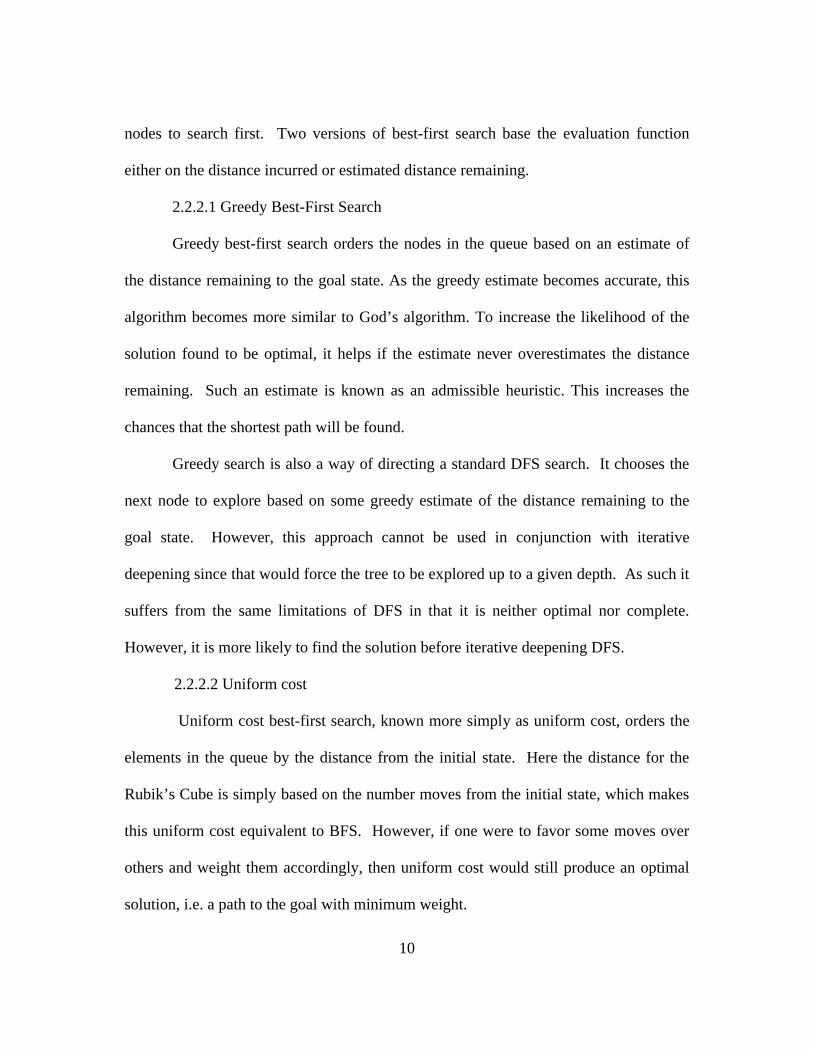
4.3 Pseudo Code for the parallel implementation
1) Initialization of the cube2) Initialization of the pattern databases3) Expand the initial node4) if(master)5) distribute the initial search limit to each of the processor6) Repeat 7) Receive request from one of the processors8) Check if goal reached 9) If(goal reached)10) Send termination message to other processors and stop11) Else12) Send next work to the requesting processor13) End if14) Search tree with the current search limit15) Until solution found or end of tree16) Else17) Receive the search limit from the master18) Check for the Exit tag19) If (exit tag)20) Stop21) End if

27
22) Search the tree with the new search limit23) If (goal reached)24) Send termination message to the master25) Else26) Request for new search limit.
Initialize the Cube
Initialize the tables
Search the treeSearch the treeSearch the tree
……………..
search limitn processors
If goal found?
Go back to search tree.
Communicate and Stop.
No Yes
Fig 4.1 Data Flow Diagram
28
CHAPTER 5
EXPERIMENTAL METHODOLOGY
We ran several experiments in the pursuit of our research. We wanted to
confirm that the algorithm we have chosen is the best fit. The program was executed for
several randomly generated test cases at varied depths. The graphs below for sequential
as well as parallel implementation are drawn for the average times of five
configurations of every depth.
5.1 Results Analysis
The aim was to carry out to extensive experimentations for different cube
configurations at various depths. The plots for the same are plotted in this chapter. All
these programs were submitted as batch programs on the UTA DPCC cluster using MPI
with C. For the sequential algorithm, configurations of depth 12-22 are tested while
results for parallel implementations are from depth 19 onwards because such higher
depths require more time and hence we need to parallelize them.
Section 5.1.1 shows graphs of execution times for the sequential implementation, and
section 5.1.2 for the parallel implementation and the comparison of the two is done in
section 5.1.3.

29
5.1.1 Results for the sequential implementation
Figures 5.1, 5.2, 5.3 are plotted to show the average time spent to get to a
solution of that particular depth. The average time is calculated for five configurations
of each depth, the times for which are listed in the corresponding tables. Figure 5.3
presents the average time Vs depth plot for all the depth from 12-22 whereas figures 5.1
and 5.2 are two parts of figure 5.3.
Average time required Vs Depth (12-18) for Reid's Sequential algorithm
0
50
100
150
200
250
10 11 12 13 14 15 16 17 18 19
Depth (12-17)
Tim
e in
se
con
ds
Series1
Fig 5.1: Average time Vs Depth (12-18) for Reid’s sequential implementation

30
Table 5.1- Data for average time Vs depth (12-18) for Reid’s sequential implementation
Average time Vs Depth (19-22) for Reid's sequential algorithm
0
50
100
150
200
250
300
350
400
450
18 19 20 21 22 23
Depth (19-22)
Tim
e in
min
ute
s
Series1
Fig 5.2: Average time Vs Depth (19-22) for Reid’s sequential implementation
Time in seconds for five configurationsDepth
Conf 1 Conf 2 Conf 3 Conf 4 Conf 5
Average time in seconds
12 103 101 101 102 100 101.314 100 103 104 100 100 101.415 103 104 100 100 101 101.616 99 101 100 99 100 99.817 315 104 104 118 114 15118 379 166 157 155 142 199.8

31
Table 5.2- Data for average time Vs depth (19-22) for Reid’s sequential implementation
Average time Vs Depth for Reid's sequential algorithm
0
5
10
15
20
25
10 11 12 13 14 15 16 17 18 19 20 21 22 23 24
Th
ou
san
ds
Depth
Tim
e in
se
con
ds
Series1
Fig 5.3: Average time Vs Depth for Reid’s sequential implementation
Time in minutes for five configurationsDepth
Conf 1 Conf 2 Conf 3 Conf 4 Conf 5
Average time in minutes
19 17.38 5.28 3.71 9.56 3.95 7.1220 3.23 36.48 88.53 255 236 123.8521 32.51 223.6 27.05 277.36 464.61 205.0322 97.66 676.16 - - - 386.91

32
5.1.2 Results for the parallel implementation
The configurations tested for serial implementation were all tested for the
parallel implementation too. Table 6.3 presents the times for five configurations for
every depth form 19-22 and the average time in minutes.
Table 5.3- Data for average time Vs depth (19-22) for the parallel implementation using np=8
Average time Vs Depth for the parallel implementation
0
50
100
150
200
250
300
350
18 19 20 21 22 23
Depth
Ave
rag
e ti
me
in m
inu
tes
Series1
Fig 5.4: Average time Vs Depth for the parallel implementation with np=8
Time in minutes for five configurationsDepth
Conf 1 Conf 2 Conf 3 Conf 4 Conf 5
Average time in minutes
19 8.38 2.36 2.08 1.68 3.86 3.3820 1.93 19.48 47.2 124.93 107.5 60.2421 24.2 160.64 3.13 180.06 213.93 116.3922 307.5 - - - - 307.05

33
5.1.3 Comparisons
It can be observed that out of the depths for which the program was run, it has
started taking considerable time after depth equal to 19. A parallel programs execution
time or wall-clock time as it is referred to be an obvious performance measure. This
time is the time elapsed from when the first processor starts executing a problem to
when the last processor completes execution. The graphs show some unpredictable
results as far as the relation between time taken and the number of processors is
concerned. One of the reasons for this peculiarity is the solution found by that particular
processor for the given configuration being different. As mentioned above since the
processors search the tree with different search limits for the IDA*, the solution found
could be different. But the most important factor here is the time gained while doing a
parallel search and hence the speedup achieved, which is considerable in most of the
cases.
The behavior or performance of a parallel program depends on various
variables like the number of processors, the size of the data being used for the
experiments, the interprocessor communications limit and also the available memory
among others. We have experimented with different numbers of processors but the size
of data remains the same for any input given. As far as the memory is concerned, the
use of UTA cluster has helped us look over this concern but the communication still
needs to be taken care of.

34
Time required in minutes to solve the Cube
1
10
100
1000
1 2 3 4 5 6 7 8
8 configurations of depth 21
Tim
e in
min
ute
s
Sequential
np=2
np-4
np=6
np=8
Fig 5.5: Comparisons of time in minutes required to solve the cube for 8 random
cubes of depth 21
The chart in fig.5.5 shows comparisons for execution times in solving a position created
by applying a sequence of moves to a solved cube. These times are as required in
obtaining an optimal solution to solve the Cube whereas the chart in fig.5.6 is a similar
graph but showing execution times in solving the inverse of the configurations used in
the fig 5.5. Both the graphs show that there is a definite time efficiency obtained in
solving the Cube or inverse in a parallel manner. The speedup achieved is even better
when the number of processors being as large as 8.

35
Time in minutes to solve the inverse
1
10
100
1000
10000
1 2 3 4 5 6 7 8
Configurations
Tim
e in
min
ute
s
Sequential
np=2
np=4
np=6
np=8
Fig 5.6: Comparisons of time in minutes required to solve the inverse for 8 random cubes of depth 21
5.1.4 Comparisons of results for the super flip configuration
Another challenge in solving Rubik’s cube is the “Super flip” configuration, in
which the edges are flipped in place. This configuration is said to provide a solution
after 24 moves and is supposedly the hardest one. Below is the comparison of times
required to solve this configuration using the sequential approach and the amount of
time saved by using the parallel implementation.

36
Time in HOURS Vs Number of processors for the Superflip Configuration
0
10
20
30
40
50
60
0 1 2 3 4 5 6 7 8 9
Number of processors (np)
Tim
e in
ho
urs
Series1
Fig 5.7: Time in hours required to solve the super flip position Vs Number of processors used
Table 5.4- Data for Time in hours Vs Number of processors required to solve the Super Flip position
Algorithm Time required to solve the Cube in hours
Sequential 51.94972np=2 43.63417np=4 40.55639np=6 27.87778np=8 22.23417
Note: np= Number of processors used in the parallel implementation.

37
CHAPTER 6
CONCLUSIONS
Although a lot of work has been done in order to achieve an optimal solution for
the Rubik’s cube, finding an optimal solution has been a difficult task. After
researching the Rubik’s puzzle and its solutions using heuristics search, it is clear that
along with speed, memory efficiency is the most important factor to be looked at. IDA*
fits the criteria of a search algorithm providing an optimal solution without larger space
complexity. However in searching for the best heuristic to solve the cube, we
incorporated the pattern database approach to achieve an optimized solution to the
Rubik’s cube in the shortest time.
But this approach uses a static pattern database; improvement can be done to
this algorithm by using disk storage for the database. This will eliminate the time for
initializing the pattern database for every run. Its performance is inversely proportional
to the memory requirements. Thus populating the pattern database with numerous
patterns would help in improving the performance. Also the symmetry factor does seem
to help pruning since the results show that the number of nodes generated for any depth
are large in case of asymmetry.
38
Along with these improvements that we plane to make in this algorithm, the
other main challenge in solving Rubik’s cube is the “Super flip” configuration, in which
the edges are flipped in place. This configuration is said to provide a solution after 24
moves and is supposedly the hardest one. We plan to solve this configuration using the
improved pattern database approach.
Parallel processing is used to address the high computation effort required by
this particular problem at greater depths. This will further help in boosting the
performance. The long term objective of this project is to use a grid for any other puzzle
solving problem including the Rubik’s Cube.

39
APPENDIX A
SEARCH TREE SIMULAITON

40
Depth ‘10’ processor‘0’
…...
Depth ‘9’ processor ‘1’
Depth ‘8’ processor ‘0’
Depth ‘7’ processor ‘3’
Depth ‘6’ processor ‘0’
Depth ‘5’ processor ‘1’
Depth ‘4’ processor ‘3’
Depth ‘3’ processor ‘3’
Depth ‘2’ processor ‘2’
Depth ‘1’ processor ‘1’
X Initial configuration
F(X) B(X) L’(X) D2(X)…... ….. U2(X)
F(Y) Z=U(Y) L’(Y) R’(Y) D2(Y)
U2 (Z)
…... …... U2(Y)
D2 (Z)L’ (Z)B (Z)A=F(Z) …... …...
B (A)F (A) U2 (A) D2 (A)…... …...L’ (A)
F (C) B (C) L’ (C) E=R’ (C) U2 (C) D2 (C)
F (E) G=U (E) L’ (E) D2 (E)…... ….. U2 (E)
F (G) D2 (G)
U2 (H)
…... …... U2 (G)
D2 (H)B (H)F (H) …... …...
B (I)J=F (I) U2 (I) D2 (I)…... …...L’ (I)
F (J) B (J) U2 (J) D2 (J)
L’ (G)
I=L’ (H)
B’ (I)
R’ (H)
R’ (G)
R’ (E)
C=B’(A)
R’ (Z)
Y=R’(X)
…... L’ (J)
H=D (G)
K=B’ (J)

41
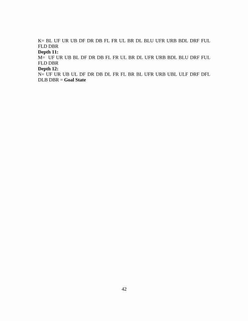
In the following tree simulation assume:
Initial configuration: X = RB RD FD FR BU BL LF LU BD UR DL FU FUL FLD FDR FRU BLU BUR BRD BDL
The path to the goal node comprises of the following intermediate configurations be:
Depth 1:Y=DB RD FD FR RU BL LF LU UB BR DL FU LUB FLD FDR LFU RBU RUF BRD BDLDepth 2: Z= DL FD FR RB BU BD LF LU RD UR BL FU DLB FDR FRU DFL ULF BUR BRD UBLDepth 3: A= RU FD FR RB DR BD LF LU LD UB BL FU FLD FDR FRU RBU BDL LFU BRD UBLDepth 4: C= RU FD UF RB DR BD LB LU LD UB RF FL FLD UFR RDB RBU BDL LFU LUB DRF Depth 5: E= RU RF UF RB DR LD LB LU FD UB BD FL RUF RFD RDB RBU LDF LFU LUB LBD Depth 6: G= RF UF RB RU DR LD LB LU FD UB BD FL RFD RDB RBU RUF LDF LFU LUB LBDDepth 7: H= RF UF RB RU LU DR LD LB FD UB BD FL RFD RDB RBU RUF LFU LUB LBD LDFDepth 8: I= RF UF RB UB LU DR LD FL FD LB BD RU RFD RDB FRU UBL LFU DLB BUR LDF
Depth 9: J= BL UF RB UB DF DR LD FL FR UL BD RU BLU RDB FRU BDL DRF FUL BUR LDFDepth 10:
F (K) U2 (K) D2 (K)…... …...L’ (K)
F (M) B (M) B’ (M) D2 (M)
B’ (K)M=U (K)
…... N=L’ (M) …... U2 (M)
Depth ‘11’ processor‘3’
Depth ‘12’ processor‘0’
42
K= BL UF UR UB DF DR DB FL FR UL BR DL BLU UFR URB BDL DRF FUL FLD DBRDepth 11:M= UF UR UB BL DF DR DB FL FR UL BR DL UFR URB BDL BLU DRF FUL FLD DBRDepth 12: N= UF UR UB UL DF DR DB DL FR FL BR BL UFR URB UBL ULF DRF DFL DLB DBR = Goal State
43
APPENDIX B
PROGRAM EXECUTION MODULE

44
Processors received = 4Script running on host node9.clusterPBS NODE FILEnode9.clusternode8.clusternode7.clusternode6.clusterStart time: 0.158430 secsusing quarter turn metricusing symmetry reductionsonly finding one solution
initializing transformation tablesinitializing distance table ... this will take several minutesdistance positions (quotient) 0q 1 ( 1) 1q 4 ( 1) 2q 34 ( 3) 3q 312 ( 24) 4q 2772 ( 185) 5q 24996 ( 1633) 6q 225949 ( 14708) 7q 2017078 ( 130032) 8q 17554890 ( 1124165) 9q 139132730 ( 8868078) 10q 758147361 (48182278) switching to backwards searching 11q 1182378518 (75087495) 12q 117594403 ( 7498528) 13q 14072 ( 1279)
Getting cube (Ctrl-D to exit):RU UF LF LU RB RD LB DB FR BU FD DL RUF LDF LFU LUB RDB RBU LBD RFDasymmetric position
Hello world from node: process 0 of 4depth 4q completed ( 18 nodes, 0 tests)solfoud:0 Start time: 0.107394 secs)
Hello world from node: process 1 of 4

45
depth 1q completed ( 12 nodes, 0 tests) (time: 108.921634 secs)solfoud:0 Start time: 0.056627 secs)
Hello world from node: process 2 of 4depth 2q completed ( 18 nodes, 0 tests) (time: 108.921944 secs)solfoud:0
Hello world from node: process 0 of 4depth 6q completed ( 18 nodes, 0 tests)
Hello world from node: process 0 of 4depth 8q completed ( 18 nodes, 0 tests)
Hello world from node: process 1 of 4depth 5q completed ( 18 nodes, 0 tests) (time: 108.922071 secs)solfoud:0
Hello world from node: process 0 of 4depth 10q completed ( 45 nodes, 0 tests)
Hello world from node: process 1 of 4depth 9q completed ( 18 nodes, 0 tests) (time: 108.922195 secs)solfoud:0
Hello world from node: process 2 of 4depth 7q completed ( 18 nodes, 0 tests) (time: 108.922364 secs)solfoud:0
Hello world from node: process 1 of 4depth 11q completed ( 126 nodes, 0 tests) (time: 108.922577 secs)solfoud:0
Hello world from node: process 0 of 4depth 12q completed ( 1,693 nodes, 2 tests)solfoud:0 Start time: 0.006165 secs)
Hello world from node: process 3 of 4depth 3q completed ( 18 nodes, 0 tests) (time: 108.930303 secs)solfoud:0
Hello world from node: process 1 of 4depth 13q completed ( 12,513 nodes, 10 tests)

46
(time: 108.932165 secs)solfoud:0
Hello world from node: process 0 of 4depth 14q completed ( 101,902 nodes, 96 tests)
Hello world from node: process 1 of 4depth 15q completed ( 778,574 nodes, 446 tests) (time: 109.466568 secs)solfoud:0
Hello world from node: process 0 of 4depth 16q completed ( 6,192,097 nodes, 3,280 tests)
Hello world from node: process 1 of 4depth 17q completed ( 50,023,079 nodes, 21,866 tests) (time: 143.674447 secs)solfoud:0
Hello world from node: process 0 of 4depth 18q completed ( 413,618,183 nodes, 153,812 tests)solfoud:0
Hello world from node: process 1 of 4 F U R U' L' U' R2 U' R F' R' F B' R U' L D' L' (19q*, 18f)
Rank 1 found the solution after time2: 414.972172
Fri Oct 28 15:33:51 CDT 2005

47
APPENDIX C
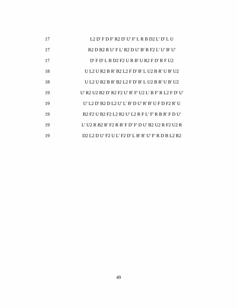
PATTERNS USED FOR EXPERIMENTATION

48
Depth Patterns
12 F2 D F2 D2 L2 U L2 U' L2 B D2 R2
12 D' L' R' B F D' U' L' R' B' F' U'
12 L U' B F' L D' U' R B F' U' R
12 F2 D F2 D2 L2 U L2 U' L2 B D2 R2
13 F' U' L' B' F' R' U' D B R2 U B R
13 F R D F2 R' U' D B L' R' F' D' R'
14 D2 L D' B' D L' D2 U2 R' U F' U' R U2
14 R2 U' R2 F' R U R' F' L' D' B' L2 F U
14 F' U' F2 L' U B' L F U' R' F' L F2 R2
14 L B2 D R B' F D' L' R D' U F' R2 U'
14 U' R' F R D2 F D2 R F' R U' R2 F' U2
14 F2 U' R2 F2 R F D2 U L B2 D2 B' D' L'
14 B' R' D F' D2 F R2 D2 F' U2 F R' D F
15 U' R2 F2 U2 L' D2 B' L2 U' L2 D2 L U2 F' U2
16 F2 D' R2 D' L' U' L' R B D' U B L F2 L U2
16 B2 D B U L R' B' F' R' B' R' D U' L' U' L
16 L U B2 L2 D2 B U B' D' R' B' F' U2 B2 U R
16 D' L' F2 L2 B F D R F L' F' R2 U2 F2 L' U'
16 R2 B2 U' R U2 B' R B' L F D F2 L2 D' L B
17 U B2 F2 D' R L U' R L D B' F' U' R L B F
49
17 L2 D' F D F' R2 D' U' F' L R B D2 L' D' L U
17 R2 D B2 R U' F L' R2 D U' B' R F2 L' U' B' U'
17 D' F D' L B D2 F2 U R B' U R2 F D' R F U2
18 U L2 U R2 B R' B2 L2 F D' B' L U2 B R' U B' U2
18 U L2 U R2 B R' B2 L2 F D' B' L U2 B R' U B' U2
19 U' R2 U2 B2 D' R2 F2 U' R' F' U2 L' B F' R L2 F D' U'
19 U' L2 D' B2 D L2 U' L' B' D U' R' B' U F D F2 R' U
19 B2 F2 U B2 F2 L2 R2 U' L2 R F L' F' R B R' F D U'
19 L' U2 R B2 R' F2 R B' F D' F' D U' B2 U2 R F2 U2 R
19 D2 L2 D U' F2 U L' F2 D' L B' R' U' F' R D B L2 R2

50
APPENDIX D
PROFILING OUTPUT

51
The profiles of the MPI program is obtained using a profiling software named
upshots. To see the profile, an alog file is created and is then displayed using the
logviewer program. The profiles show the time distribution and the communication
across the processors.

52
REFERENCES
[1] Culberson, J.C., and Schaeffer, J., “Searching with Pattern Databases,”
Proceedings of the 11th conference of the Canadian society for the
computational study of intelligence, Springer Verlag, 1996.
[2] David Singmaster Notes on Rubik’s magic cub, Hillside, New Jersey, 1980.
[3] Keith, H.R., “Solving Rubik’s Cube,” NE, pp. 43-207.
[4] Korf, R.E., “Depth-First Iterative-Deepening: An Optimal Admissible Tree
Search,” Artificial Intelligence, 1985, Vol. 27, pp. 97-109.
[5] Korf, Richard. “Finding optimal solutions to Rubik's Cube using pattern
databases”, Proceedings of the Fourteenth National Conference on Artificial
Intelligence (AAAI-97), Providence, RI, pp. 700-705, July 1997
[6] Study Report titled “Implementing an IDA* search on a cluster of workstations
to solve a Rubik’s cube” by Sameer Abhyankar and Bimal Tandel. University
of Texas at Arlington.
[7] Thesis report by Joe Fowler, University of Colorado in Boulder,1995
[8] Culberson, Joseph C. and Schaeffer, Jonathan. Searching with Pattern
Databases. Canadian Conference on AI, 1996, pp. 402-416.

53
[9] Culberson, Joseph C. and Schaeffer, Jonathan.. Efficiently searching the 15-
puzzle. Technical report, Department of Computer Science, University of
Alberta, 1994.
[10] Hecker, David and Banerji, Ranan. The Slice Group in Rubik's Cube.
Mathematics Magazine, Vol. 58, No. 4, pp. 211-218, September 1985.
[11] Joyner, David. Adventures in group theory: Rubik's Cube, Merlin's Machine,
and Other Mathematical Toys. Johns Hopkins University Press, April 2002.
[12] Korf, Richard; Reid, Michael; and Edelkamp, Stefan. Time complexity of
Iterative-Deepening A*, Artificial Intelligence, Vol. 129, No. 1-2, pp. 199-218,
June 2001.
[13] Singmaster, David. Notes of the Rubik’s Magic Cube. Enslow, 1981.
[14] Butler, Gregory. Fundamental Algorithms for Permutation Groups. Springer-
Verlag, 1991.
[15] Egner, Sebastian and Püschel, Markus. Solving Puzzles related to
Permutation Groups. Proceedings of the International Symposium on Symbolic
and Algebraic Computing (ISSAC), 1998
[16] Korf, Richard. Sliding-tile puzzles and Rubik's Cube in AI research, IEEE
Intelligent Systems, pp. 8-12, November 1999.

54
[17] Korf, Richard. Depth-first iterative-deepening: An optimal admissible tree
search, Artificial Intelligence, Vol. 27, No. 1, pp. 97-109, 1985
[18] Rotman, Joseph J. An Introduction to the Theory of Groups, 4th Edition.
Springer-Verlag, 1995.
[19] Russell, Stuart and Norvig, Peter. Artificial Intelligence, A Modern Approach.
Prentice-Hall, 1995.
[20] Schönert, Martin et. al. Cube Lover’s Index by Date. http://www.math.rwth-
aachen.de/~Martin.Schoenert/Cube-Lovers/
[21] http://jeays.net/rubiks.htm
[22] http://www.cs.princeton.edu/~amitc/Rubik/solution.html
[23] http://www.rubiks.com, Rubik/ Seven towns, 1998
[24] http://home.t-online.de/home/kociemba/cube.htm
[25] http://www.math.ucf.edu/~reid/Rubik/
[26] http://www.math.rwthachen.de/~Martin.Schoenert/CubeLovers/Mark_Longri
dge__Superflip_24q.html

55
BIOGRAPHICAL INFORMATION
Miss.Aslesha Nargolkar is born on 26th April 1982 in the city of Pune, Maharashtra in
India. She completed her high school education in Muktangan English School in 1997
and in 2003 she graduated with a Bachelors degree in Computer Engineering from the
Pine University in Maharashtra, India with a first class. She started pursuing her
Masters degree in Computer Science and Engineering in fall’2003. She did research in
“Paralllel Processing the Rubik’s Cube “under the supervision of Dr. Ahmad. In future
she plans to pursue a PhD degree.