Embed Size (px)
Citation preview

Solving Rubik’s Cube with Non-Standard Moves
L A U R E N T V A N E E S B E E C K
Master of Science Thesis Stockholm, Sweden 2014


Solving Rubik’s Cube with Non-Standard Moves
L A U R E N T V A N E E S B E E C K
Master’s Thesis in Mathematics (30 ECTS credits) Master Programme in Mathematics (120 credits) Royal Institute of Technology year 2014
Supervisors at Université Catholique de Louvain, Belgien, was Olivier Pereira
Supervisor at KTH was Tilman Bauer Examiner was Tilman Bauer
TRITA-MAT-E 2014:55 ISRN-KTH/MAT/E--14/55--SE Royal Institute of Technology School of Engineering Sciences KTH SCI SE-100 44 Stockholm, Sweden URL: www.kth.se/sci


Université catholique de LouvainÉcole polytechnique de Louvain
Louvain-la-Neuve
Royal Institute of TechnologyDepartment of Mathematics
Stockholm
Thesis for the degree ofMaster in Mathematical Engineering (UCL)
Master in Mathematics (KTH)
Solving Rubik’s Cubewith Non-Standard Moves
by
Laurent Van Eesbeeck
SupervisorsOlivier Pereira (UCL)Tilman Bauer (KTH)
ReadersChristophe Petit (UCL)
Jean-Pierre Tignol (UCL)
Louvain-la-Neuve, August 2014


Abstract
Still another thesis on Rubik’s cube? Is there still something new to write onthat puzzle? In this document, we approach the cube with a rather unusual question:“how would you solve the cube if, instead of using the 6 classical rotations, you wererestricted to a set of arbitrary moves?” To answer that question, we will dive intogroup theory.
Inspired by some previous work on the factorization of the symmetric group, wehave developed an algorithm that answers our initial question. However, being ableto solve the cube with any set of moves has a trade-off: while some algorithms solvethe cube in 20 moves, ours requires several thousands.
One could go further than this thesis by: improving our algorithm, providingrigourous bounds on its complexity, or generalizing the algorithm to the n × n × ncube.


Acknowlegdments
I would like to thank my three supervisors:
• Olivier Pereira for accepting to be my official UCL supervisor;
• Tilman Bauer for his support and his questions;
• Christophe petit for his weekly support, for recentering me to the main topic andfor having endured the ups and downs of my productivity.
And of course, I would like to thank my family for their unconditional support.


Contents
Contents 7
Introduction 9
1 Required Notions in Group Theory 111.1 A Very Short Introduction to Group Theory . . . . . . . . . . . . . . . . . . 111.2 Quotient Groups and Semi-Direct Products . . . . . . . . . . . . . . . . . . 151.3 Permutation Groups . . . . . . . . . . . . . . . . . . . . . . . . . . . . . . . 181.4 Conjugated Permutations and Commutators . . . . . . . . . . . . . . . . . . 221.5 Notations and Conventions Used in this Document . . . . . . . . . . . . . . 26
2 Introducing Rubik’s Cube 272.1 Permutations, Positionings and Orientations . . . . . . . . . . . . . . . . . . 282.2 The Semi-Direct Product Behind G . . . . . . . . . . . . . . . . . . . . . . . 312.3 The Structure of G . . . . . . . . . . . . . . . . . . . . . . . . . . . . . . . . 32
3 Factorizing the Symmetric Group 373.1 Finding a Permutation of Degree Less than n/4 . . . . . . . . . . . . . . . . 393.2 Finding a 3-Cycle . . . . . . . . . . . . . . . . . . . . . . . . . . . . . . . . . 413.3 Factorizing any Target from a 3-Cycle . . . . . . . . . . . . . . . . . . . . . 47
4 Solving Rubik’s Cube with Non-Standard Moves 494.1 Factorizing Small Groups . . . . . . . . . . . . . . . . . . . . . . . . . . . . 494.2 Factorizing A8 ×A12 . . . . . . . . . . . . . . . . . . . . . . . . . . . . . . . 514.3 Solving Rubik’s Cube with Non-Standard Moves . . . . . . . . . . . . . . . 52
Conclusion and Further Work 55
Bibliography 57
A Code Snippets 59A.1 Rubik’s Cube . . . . . . . . . . . . . . . . . . . . . . . . . . . . . . . . . . . 59A.2 Babai et al’s factorization of Sn . . . . . . . . . . . . . . . . . . . . . . . . . 60A.3 Small Groups . . . . . . . . . . . . . . . . . . . . . . . . . . . . . . . . . . . 66A.4 solving Rubik’s Cube with Non-Standard Moves . . . . . . . . . . . . . . . 73
7


Introduction
Still another thesis on Rubik’s cube? Didn’t people already do this?Instead of presenting one other effective way to solve the cube or finding an alternative
proof to God’s number (the minimal number of moves with which one can solve the cubefrom any configuration), through this thesis we are interested on the following question:“how would one solve the cube if, instead of the 6 classical face rotations, he was restrictedto use an arbitrary set of moves?”
If odd, that question perfectly illustrates a far-from-trivial and deeply studied problemin group theory, the factorization problem: given a set S = {s1, . . . , sm} generating a groupG and an element g in that group G, how does one express g as a product of elements in S?(This problem can be seen as a generalized version of the discrete logarithm problem andhas potential applications in cryptography ([PQ11]). For some groups and some generatingsets, the problem has well-known solutions. But in general, there is no obvious solution.Solving Rubik’s cube is merely the tip of the iceberg of a deeper problem.
This thesis is divided into four chapters.
• Chapter 1 is a warm-up. It introduces the notions in group theory that will be usedlater on, from the basic definitions to semi-direct products and permutation groups.The main notions are recaped in Section 1.5.
• Chapter 2 introduces the group structure behind Rubik’s cube (it is a semi-directproduct) and presents a systematic strategy to solve it: first position the cubits right,then orient them right. As we will see, that solution requires about 1500 moves, faraway from the world’s record of 20 moves.
• Chapter 3 dives into the litterature and presents a solution to the factorizationproblem for the symmetric group. As we will see, the studied algorithm does notwork for small symmetric groups such as those encountered in Rubik’s cube.
• Chapter 4 is the central point of this thesis. Building upon the material presented inthe Chapters 1 to 3, it presents a solution to Rubik’s cube that works for any givenset of moves. It also provides a variant of the algorithm of Chapter 3 that worksfor small symmetric groups. Tests suggest that our algorithm requires about 6000moves for the standard moves, and about 80 000 moves for any given set of moves.
9


Chapter 1
Required Notionsin Group Theory
This chapter provides a quick reminder of the group theory notions needed to understandthe next chapters.
• Section 1.1 defines the very basic notions used in group theory: a group, a groupaction, a Cayley graph and a Schreier graph, a homomorphism and a subgroup.
• Section 1.2 presents cosets, Schreier coset graphs, normal subgroups, quotient groupsand semi-direct products; the two latter being special groups that we will encounterin Chapter 2 and 4 when studying the group structure of Rubik’s cube.
• Section 1.3 gives a wide overview of permutation groups: definition, cycle representa-tion of a permutation and its properties, parity of a permutation and decompositionof a permutation as a product of 2- and 3-cycles. Permutation groups will be usedwidely through this document and more specifically, the results of this section willbe used in Chapters 3 and 4.
• Section 1.4 presents some nice properties of conjugated permutations and the com-mutator of two permutations. These properties will be used mainly in Chapter 3.
• Section 1.5 summarizes this chapter by listing the notations and conventions usedthrough this document.
Readers familiar with all these notions may directly skip to Section 1.5; references tothe main results of this chapter will be done when necessary.
1.1 A Very Short Introduction to Group TheoryAbstract algebra is a branch of mathematics where one defines mathematical structures bygeneralizing structures we commonly use and then studying the properties of these generalobjects. Groups are fundamental objects in abstract algebra, as they are used to definemore complex objects such as rings, fields, modules, and so on.
Definition 1.1. A group (G, ?) is a set G supplied with an operator ? : G × G → Gsatisfying the following axioms:
closedness ∀g1, g2 ∈ G, g1 ? g2 ∈ G;
11

12 CHAPTER 1. REQUIRED NOTIONS IN GROUP THEORY
associativity ∀g1, g2, g3 ∈ G, g1 ? (g2 ? g3) = (g1 ? g2) ? g3;
existence of a neutral element G has an identity element Id such that ∀g ∈ G, g?Id =Id ?g = g;
existence of inverses ∀g ∈ G, ∃g−1 ∈ G such that gg−1 = g−1g = Id.
If furthermore ? satisfies
commutativity ∀g1, g2 ∈ G, g1 ? g2 = g2 ? g1
then (G, ?) is called a commutative group.
Remark. When the group operation is obvious from the context, (G, ?) is usually denotedby G and the ? symbol either is a + or is ommitted: one writes g1 + g2 (for so-calledadditive groups) or g1g2 (for so-called multiplicative groups) instead of g1 ? g2. One alsowrites g + g + · · ·+ g︸ ︷︷ ︸
n times
= ng and gg · · · g︸ ︷︷ ︸n times
= gn.
We are already familiar with different examples of groups: (R0,×) is a commutativegroup with identity 1 and as inverse r−1 = 1/r; (Z,+) is a commutative group with identity0 and as inverse z−1 = −z. (Zn,+) is the cyclic group modulo n: Zn = {0, . . . , n − 1}with operation a?b = (a+ b) mod n.1 As an example of non-commutative group, considerGL(2,R), the multiplicative group of 2× 2 matrices with non-zero determinant.
From the axioms of a group follow a couple of elementary properties. The readerinterested in a proof of these properties may consult [DF04], §1.1.
Proposition 1.2. Let G be a group. Then the following holds:
• the identity of G is unique;
• every element g ∈ G has a unique inverse g−1 and (g−1)−1 = g;
• the inverse of g1g2 is (g1g2)−1 = g−12 g−1
1 ;
• the equations ax = b and xa = b have a unique solution x ∈ G for every a, b ∈ G;
• for every g, x, y ∈ G, if gx = gy then x = y and if xg = yg then x = y.
As we will see when we study permutation groups, some group elements have niceproperties. The purpose for the moment is merely to mention their existence.
Definition 1.3. Two group elements g1 and g2 are said conjugate if there exists an h suchthat g1h = hg2. The conjugate of g by h, noted gh, is the element h−1gh.
Note that
(gh)−1 = (h−1gh)−1 = h−1g−1h = (g−1)h
gh1h2 = (h1h2)−1gh1h2 = h−12 (h−1
1 gh1)h2 = (gh1)h2
(g1g2)h = h−1(g1g2)h = (h−1g1h)(h−1g2h) = gh1gh2 .
1Observe the difference between the modulo binary operator and the modulo equivalence relation:compare 8 mod 3 = 2 (operator) and 8 ≡ 11 (mod 3) (equivalence relation). For convenience, through thisdocument the modulo operator has the same precedence as in Magma: (a + b) mod c 6= a + b mod c =a+ (b mod c) and a · b mod c = (a · b) mod c.

1.1. A VERY SHORT INTRODUCTION TO GROUP THEORY 13
Definition 1.4. The commutator of two elements g and h, noted [g, h], is defined as[g, h] = g−1h−1gh.
When g and h commute, [g, h] = Id, so the commutator can be seen as a measure of“how much” two elements commute. Indeed, gh = hg[g, h]. One also notes that
[g, h]−1 = (g−1h−1gh)−1 = h−1g−1hg = [h, g].
Groups can interact with other structures through a mechanism called group actions.
Definition 1.5. A left group action of a group G on a set S is an operation ∗ : G×S → Ssatisfying the two following actions:
• for all s ∈ S, Id ∗s = s;
• for all g, h ∈ G, s ∈ S, (gh) ∗ s = g ∗ (h ∗ s).
Similarly, a right group action is an operation ∗ : S ×G→ S satisfying
• for all s ∈ S, s ∗ Id = s;
• for all g, h ∈ G, s ∈ S, s ∗ (gh) = (s ∗ g) ∗ h.
As an example, the group operation is a (left and right) action of a group G onitself. Another example is the previously defined conjugacy operation: the operationg · h = gh = h−1gh is a right group action of G on itself. We’ll see two more examples inthe context of permutation groups.
Remark. Some authors define the conjugate of g by h as hg = hgh−1 and the commutatorof g and h as [g, h] = ghg−1h−1. With that definition, the operation h · g = hg is a leftgroup action.
Our choice of using the other convention is made to avoid confusions with Magma(Magma defines gh = h−1gh and (g, h) = g−1h−1gh) and because it is consistent with themultiplication of permutations from left to right. (More about this in Section 1.3.) Moregenerally, to be consistent with this convention, function composition must be done fromleft to right: (fg)(x) = g(f(x)). That’s why through this document, the image of x by afunction f , f(x), will be noted xf and (fg)(x) = xfg = (xf )g. The group actions we willencounter will also, by convention, be right group actions.
Definition 1.6. The order of a group G, |G|, is the number of elements in G. The orderof an element g ∈ G, |g|, is the smallest positive integer n such that gn = Id. If such aninteger does not exist, then by convention |g| =∞.
The following result gives some information on the order of an element. Again, theproof can be found in [DF04], §3.2.
Proposition 1.7. If G is a finite group, then |g| divides |G|.
One way to describe a group is to use a generating set S = {s1, s2, . . . , sn}. One thenwrites G = 〈S〉 to describe the group defined by the set of all finite products of elementsof S with respect to the implicit group operation:
G ={si1si2 · · · sik | ij ∈ {1, . . . , n} ∀j ∈ {1, . . . , k}
}.
With a particular generating set S in mind, one can define the Cayley graph of a group.Schreier graphs are similar but are constructed from a group action.

14 CHAPTER 1. REQUIRED NOTIONS IN GROUP THEORY
0
12
3
4 5
Figure 1.1: The Cayley graph of Z6 generated by {1, 2}, Γ(Z6, {1, 2}).
Definition 1.8. The (colored) Cayley graph of G with respect to a generating set S ={s1, . . . , sn}, Γ(G,S), is the oriented graph with vertex set G and edge set
{(g, gsi) | g ∈
G, i ∈ {1, . . . , n}}. In a colored Cayley graph, the vertex (g, gsi) is colored in the ith
color.
Definition 1.9. Given a group G = 〈S〉 that acts on a set X with a left (right) groupaction ∗ : G × X → X, the left Schreier graph Γ(G,S,X, ∗) is the oriented graph withvertex set X and edge set {(x, s ∗ x) |x ∈ X, s ∈ S}. The right Schreier graph has thesame vertex set and {(x, x ∗ s) |x ∈ X, s ∈ S} as edge set.
Since the group multiplication is a group action, Schreier graphs generalize Cayleygraphs. These graphs are regular (i.e., every vertex has the same number of neighbors),so they usually lead to very symmetric and structured drawings (Figure 1.1).
A group generated by a set S ⊂ G can also form a smaller group than G called asubgroup. E.G., 〈2〉 = {0, 2, 4} is a subgroup of Z6.
Definition 1.10. A subgroup H of G is a subset of G which forms a group under thegroup operation in G. If H is a subgroup of G, one writes H ≤ G.
Since the associativity of the operation is ensured for every element in G (and hencealso in H ⊂ G), one must only verify the closedness, existence of a neutral element andexistence of inverses axioms in H to check that H is a subgroup of G. Note that theidentity in H is also the identity in G. An equivalent way to show that H is a subgroupof G is the subgroup criterion. For a proof, see [DF04], §2.1.
Proposition 1.11 (The Subgroup Criterion). A subset H of a group G is a subgroup ifand only if
1. H 6= ∅
2. ∀x, y ∈ H, xy−1 ∈ H.
Definition 1.12. For G and H two groups, a map φ : G→ H is called a homomorphismif, ∀g1, g2 ∈ G,
(g1g2)φ = gφ1 · gφ2 .
A homomorphism from G to G is called an automorphism. If a homomorphism is bijective,it is called an isomorphism and G and H are said isomorphic, which is noted by G ∼= H.
One also has the following properties for homomorphisms (see [DF04], §3.1).
Proposition 1.13. For G and H two groups and for φ : G→ H,

1.2. QUOTIENT GROUPS AND SEMI-DIRECT PRODUCTS 15
• IdG φ = IdH ;
• for every g ∈ G, (g−1)φ = g(φ−1);
• kerφ = {g ∈ G | gφ = Id} is a subgroup in G;
• Imφ = Gφ = {gφ | g ∈ G} is a subgroup in H.
Remark. Two isomorphic groups G and H can be seen as the same group up to the differ-ence that its elements have different names from one group to another. The isomorphismlinking these groups has the effect of “translating” an element of G to its equivalent in H.
1.2 Quotient Groups and Semi-Direct ProductsLet us first review some results related to subgroups. Closely related to a subgroup is thenotion of a coset.
Definition 1.14. For H ≤ G a subgroup of G and g ∈ G, gH = {gh |h ∈ H} is called aleft coset of H and Hg = {hg |h ∈ H} is a right coset. The elements of a coset are calledits representatives.
Remark. Needless to say, what we say in this section is written with left cosets but canjust as well be written in terms of right cosets.
Two cosets of a same subgroup either are disjoint or are identical, and the set of cosetsof a particular subgroup H ≤ G form a partition of G. Note also for all g′ ∈ gH, gH = g′H(see [DF04], §3.1). This implies that all the cosets have the same number of elements. Onenotes [G : H], the index of H in G, as the number of distinct cosets H has in G. Hence,when G is finite, [G : H] = |G|/|H|.
Cosets have an equivalent links with graph theory as Cayley graphs and Schreiergraphs: Schreier coset graphs.
Definition 1.15. Given a group G = 〈S〉 and a subgroup H ≤ G, the Schreier leftcoset graph Γ(G,S,H) is the oriented graph with vertex set {gH | g ∈ G} and edge set{(gH, sgH) | g ∈ G, s ∈ S}. The Schreier right coset graph is the graph with vertex set{Hg | g ∈ G} and edget set {(Hg,Hgs) | g ∈ G, s ∈ S}.
For this section we need some particular subgroups called normal subgroups.
Definition 1.16. A subgroup N ≤ G is said normal if for all g ∈ G, n ∈ N ,
g−1ng ∈ N.
If N ≤ G is normal, one notes N E G.
Normal subgroups and kernels of homomorphisms are related. From [DF04], §3.1,
Proposition 1.17. A subgroup N ≤ G is normal if and only if it is the kernel of somehomomorphism.
One main result in group theory is that the set of distinct cosets of a normal subgroup,{gN | g ∈ G}, forms a group with the group operation
(g1N) · (g2N) = g1g2N.

16 CHAPTER 1. REQUIRED NOTIONS IN GROUP THEORY
In other words: to multiply two cosets, take any element n1 ∈ g1N and any elementn2 ∈ g2N ; the coset (g1N)(g2N) is the coset to which belongs n1n2. We won’t showhere that this operation is well-defined, i.e., that the result of this operation is the sameindependently of the choice of representatives. (The interested reader can consult [DF04].)
An equivalent approach of this operation is the following. Suppose that there is ahomomorphism φ : G → H such that φ is a one-to-one relation between the cosets gNand the elements of H: for every g, for every n ∈ gN , nφ = h and h is uniquely and onlydetermined by g. (This implies that Nφ = Id, i.e., that N is the kernel of φ.) Then theproduct of two cosets works as follows: for g1N and g2N , take the corresponding h1 andh2 in H, and compute h1h2. The coset (g1N)(g2N) is the one corresponding to h1h2.
The group of cosets of N ≤ G supplied with the previously defined operation is calledthe quotient group G/N . Its identity is the coset IdN = N and the inverse of gN is(gN)−1 = g−1N .
To clarify this with an example, consider the normal subgroup of Z, 3Z = {. . . ,−3, 0, 3, 6, . . . }.It has three distinct cosets: 0+3Z, 1+3Z = {. . . ,−2, 1, 4, . . . }, 2+3Z = {. . . ,−1, 2, 5, . . . }.3Z is also the kernel of the homomorphism φ : Z → Z3, x 7→ x mod 3. One can then add1 + 3Z and 2 + 3Z in two different ways:
• one can choose 7 ∈ 1 + 3Z and 5 ∈ 2 + 3Z. Their sum, 7 + 5 = 12 lies in 0 + 3Z,hence (1 + 3Z) + (2 + 3Z) = 0 + 3Z.
• φ maps 1 + 3Z to 1 and 2 + 3Z to 2. In the group Z3, 1 + 2 = 0 and 0 is associatedto the coset 0 + 3Z. Hence, (1 + 3Z) + (2 + 3Z) = 0 + Z.
These two ways to multiply cosets in a quotient group are summarized in what isknown as the first isomorphism theorem (see [DF04], §3.3).
Theorem 1.18. If φ : G→ H is a group homomorphism, then kerφ is a normal subgroupand G/ kerφ ∼= Imφ.
We can now move to the last topic: direct and semi-direct products.
Definition 1.19. The direct product between two groups (G1, ?) and (G2, ∗), noted G1×G2, is the set {(g1, g2) | g1 ∈ G1, g2 ∈ G2} supplied with the operation
(g1, g2) · (g′1, g′2) = (g1 ? g′1, g2 ∗ g′2).
It is not difficult to check that (G1 × G2, ·) is a group. Closedness and associativityare inherited properties from G1 and G2, it has (IdG1 , IdG2) as identity and (g1, g2)−1 =(g−1
1 , g−12 ).
The notion of semi-direct product is a generalization of the direct product. To introduceit, consider a group G with a normal subgroup N E G. If g1 and g2 ∈ G can be writtenas h1n1 and h2n2 for some n1, n2 ∈ N , then
g1g2 = (h1n1)(h2n2) = h1h2(h−12 n1h2)n2
But since N is normal, h−12 n1h2 = n′1 ∈ N . Hence,
(h1n1)(h2n2) = (h1h2)(n′1n2)
The following definition of the semi-direct product contains a homomorphism φ : H →Aut(N). Here, Aut(N) is the group of all the homomorphisms from N to N with asgroup operation the composition of functions: for f, g ∈ Aut(N), f · g is the function

1.2. QUOTIENT GROUPS AND SEMI-DIRECT PRODUCTS 17
x 7→ xfg = (xf )g. (Observe that with quotient groups we introduced groups of sets, herewe introduce a group of functions.) The homomorphism φ : H → Aut(N) hence meansthat
• for every h ∈ H, φ(h) is a homomorphism from N to N : (n1n2)φ(h) = n1φ(h) ·n2
φ(h);
• for h1, h2 ∈ H, φ(h1h2) is the homomorphism n 7→ nφ(h1h2) = (nφ(h1))φ(h2);
• φ(Id) is the identical homomorphism: nφ(Id) = n.
With this example in mind, we can now state the definition of a semi-direct product.
Definition 1.20. Given two groups H and N and a homomorphism φ : H → Aut(N), thesemi-direct product HnφN is the set {(h, n) |h ∈ H, n ∈ N} supplied with the operation
(h1, n1) · (h2, n2) = (h1h2, n1φ(h2)n2).
In the introductary example, nφ(h) = h−1nh = nh. For a direct product, φ(h) is theidentity automorphism: nφ(h) = n.
The semi-direct product is a group:
• Closedness is obvious.
• Associativity: [(h1, n1)(h2, n2)
](h3, n3) =
(h1h2, n1
φ(h2)n2)(h3, n3)
=(h1h2h3,
(n1
φ(h2)n2)φ(h3)
n3)
= (h1h2h3, n1φ(h2h3)n2
φ(h3)n3)(h1, n1)
[(h2, n2)(h3, n3)
]= (h1, n1)(h2h3, n2
φ(h3)n3)= (h1h2h3, n1
φ(h2h3)n2φ(h3)n3).
• Existence of a neutral element: (Id, Id) is the neutral element of the group. Indeed,
(h, n)(Id, Id) = (h · Id, nφ(Id) · Id) = (h, n)(Id, Id)(h, n) = (Id ·h, Idφ(h) ·n) = (n, h).
• Existence of inverses: (h, n)−1 =(h−1, (n−1)φ(h−1)). Indeed,
(h, n)(h−1, (n−1)φ(h−1)) =
(hh−1, nφ(h−1) · (n−1)φ(h−1))
= (Id, (nn−1)φ(h−1)) = (Id, Id)(h−1, (n−1)φ(h−1))(h, n) = (h−1h,
((n−1)φ(h−1))φ(h) · n)
= (Id, (n−1)φ(h−1h) · n) = (Id, Id).
The discussion behind the introductory example is summarized in the following theo-rem.
Theorem 1.21 ([DF04], §5.5). Suppose G is a group with N,H two subgroups of G suchthat every g ∈ G can be written as a product nh for some n ∈ N,h ∈ H. If N E G andN ∩H = {Id}, then G ∼= H nφN where φ : H → Aut(N) maps n 7→ nφ(h) = h−1nh = nh.

18 CHAPTER 1. REQUIRED NOTIONS IN GROUP THEORY
Remark. When one follows the convention that nh = hnh−1, the reasoning in the intro-ductory example becomes
(n1h1)(n2h2) = n1(h1n2h−11 )h1h2 = (n1n2
h1)(h1h2)
and the definition of the semi-direct product naturally becomes
N oφ H ={(n, h) ∈ N ×H | (n1, h1) · (n2, h2) = (n1n2
φ(h1), h1h2)}.
To make the difference between these definitions, one uses either the sign n or o.
1.3 Permutation GroupsPermutation groups are among the most common finite groups and are closely linked tothe notion of symmetry.
Definition 1.22. A permutation on a set A is a bijection from A to A. The set ofall permutations on A, supplied with the function composition, is a group called SA. IfA =
{1, . . . , n
}, SA is called Sn.
Proposition 1.23. SA is a group.
Proof. One needs to check the axioms of a group:
1. ∀f, g ∈ SA, fg ∈ SA: true since the composition of two bijections is still a bijection;
2. ∀f, g, h ∈ SA, (fg)h = f(gh): true since the function composition is associative;
3. SA has an identity element: the identity function Id : x 7→ x is a bijection and∀f ∈ SA, f · Id = Id ·f = f ;
4. every f ∈ SA has an inverse: true since f is a bijection.
Note, however, that SA is not commutative. Through this document, we will onlyconsider permutation groups over the finite set
{1, . . . , n
}.
For a given permutation f ∈ Sn, one notes xf the image of x ∈ {1, . . . , n} by f . Thisinduces the natural right group action ∗ : {1, . . . , n} × Sn → {1, . . . , n}, x ∗ f = xf . It isa group action:
x ∗ Id = xId = x, x ∗ (fg) = xfg = (xf )g = (x ∗ f) ∗ g.
Permutations also naturally act on vectors by the right group action ∗ : Rn × Sn →Rn, (x1, . . . , xn) ∗ f = (x(1f ), . . . , x(nf )). One then naturally notes (x1f , . . . , xnf ) =(x1, . . . , xn)f .
The previous action is particular because it also defines a homomorphism φ : Sn →Aut(Rn) which maps x → xφ(f) = xf . (Note that every homomorphism φ : G → Aut(H)induces a group action of G on H but that the converse is not true in general.) It is ahomomorphism because
(x+ y)f = (x1 + y1, . . . , xn + yn)f = (x1f + y1f , . . . , xnf + ynf ) = xf + yf .
Hence, from the previous section, the group
{(x, f) ∈ Rn × Sn | (x1, f1) · (x2, f2) = (x1 + x2f1 , f1f2)}
is a semi-direct product.

1.3. PERMUTATION GROUPS 19
Definition 1.24. A permutation group G ≤ Sn is said k-transitive if for every pair ofk-tuples (t1, . . . , tk) and (t′1, . . . , t′k) with ti 6= tj and t′i 6= t′j for every i 6= j, there exists apermutation f ∈ G such that f(t1) = t′1, . . . , f(tk) = t′k. A 1-transitive permutation groupis said transitive.
Definition 1.25. The support of a permutation f , supp(f), is the set of elements in{1, . . . , n
}that are moved by f . The degree of f , deg f , is the number of elements that it
moves.
Note that supp(f) = supp(f−1) and that deg(f) = deg(f−1). Also, if = i if and onlyif i 6∈ supp(f).
The most straightforward way to represent a permutation is the line representation:put the elements a ∈ A on a first line and put their corresponding values f(a) on a secondline. For example, in S4, the function f mapping 1 to 3, 2 to 4, 3 to 2 and 4 to 1 isrepresented as
f =(
1 2 3 43 4 2 1
).
Multiplying two functions with this representation is straightforward too. For example, ifg maps 1 to 4, 2 to 3, 3 to 2 and 4 to 1,
fg =(
1 2 3 43 4 2 1
)·(
1 2 3 44 3 2 1
)
=(
1 2 3 42 1 3 4
)
However, the line representation is quite heavy. A more popular one is the cyclerepresentation: in the previous example, f maps 1 to 3, 3 to 2, 2 to 4 and 4 to 1, so itscycle representation is
f = (1, 3, 2, 4).
As a second example, g maps 1 to 4 and 4 to 1; 2 to 3 and 3 to 2, which makes 2 distinctcycles:
g = (1, 4)(2, 3).
As a third example, the product fg is
fg = (1, 2)(3)(4);
however, since the cycles (3) and (4) do not carry any relevent information, they areomitted from the representation:
fg = (1, 2).
The cycle representation of a permutation is unique up to a reordering of its cycles,
g = (1, 4)(2, 3) = (2, 3)(1, 4),
and up to starting each cycle with another element of the cycle:
f = (1, 3, 2, 4) = (3, 2, 4, 1) = (2, 4, 1, 3) = (4, 1, 3, 2).
We can then count the number of permutations of a particular cycle structure.

20 CHAPTER 1. REQUIRED NOTIONS IN GROUP THEORY
Proposition 1.26. Write n = 1n1 + 2n2 + · · ·+ knk. There are
n!∏ki=1 i
nini!
different permutations that have n1 1-cycles, n2 2-cycles, . . . , nk k-cycles.
Proof. We can represent every permutation as a string containing all the integers 1, . . . , nexactly once and split these strings according to the fixed cycle structure. (This represen-tation explicitly includes the 1-cycles.) There are n! such strings.
But amongst these strings, some are equivalent representations of the same permuta-tions:
• every k-cycle can be written in k equivalent different ways, which makes a totalfactor
∏i ini ;
• in this string representation, we can swap cycles of same length among them: e.g.,for n = 9, n1 = n2 = 1 and n3 = 2, the strings
123 45 6 789 and 789 45 6 123
represent the same permutation. This makes the factor∏i ni!.
Multiplying two permutations from their cycle representation is a bit less obvious andis given by the following algorithm.
1. Start a new cycle with the smallest element x in supp(f)∪ supp(g) that hasn’t beenused yet.
2. Do this for every cycle in the product, starting from the cycle on the left and movingto the right: if x belongs to the cycle, replace x by the element next to it in thecycle.
3. If the new x is equal to the first element of the cycle under construction, close thatcycle and go to step 4. Else, add x to the current cycle, add it to the list of elementsalready used and go back to step 2.
4. If the list of elements that haven’t been used yet is empty, remove the 1-cycles; thealgorithm is done. Else, go back to step 1.
As an example, consider the product f2g = ffg with f and g defined as previous:
f2g = (1, 3, 2, 4)(1, 3, 2, 4)(1, 4)(2, 3).
The multiplication algorithm goes as follows. First, start a new cycle with 1. In the firstcycle, 1 goes to 3. In the second cycle, 3 goes to 2. 2 does not appear in the third cycle,so it remains 2. In the fourth cycle, 2 goes to 3. Hence,
f2g = (1, 3 . . .
In the first cycle, 3 goes to 2. In the second, 2 goes to 4. In the third, 4 goes to 1. 1 doesnot appear in the fourth cycle, closing the first cycle of the product:
f2g = (1, 3) . . .

1.3. PERMUTATION GROUPS 21
We then start a new product with an element that hasn’t been used yet: 2. In the firstcycle, 2 goes to 4. In the second, 4 goes to 1. In the third, 1 goes to 4. 4 does not appearin the last cycle. Then,
f2g = (1, 3)(2, . . .
One easily checks that 2 goes to 4, closing so the second cycle:
f2g = (1, 3)(2, 4).
The cycle representation is convenient to extract some characteristics of a permutation.Indeed, the support of a permutation is the set of elements in its cycle representation andits degree is the number of elements in it. It also makes the following result trivial.
Proposition 1.27. Every permutation of Sn can be written as a product of disjoint cycles.
From the algorithm of multiplication between permutations, we also have that
Proposition 1.28. Disjoint cycles commute.
In addition of providing a compact representation of permutations, the cycle represen-tation of a permutation gives some information about its order.
Proposition 1.29. The order of a k-cycle is k.
Proof. Observe that (a0, . . . , ak−1)n is a permutation that sends ai to a(i+n) mod k. Hencen = k is the smallest positive power such that (a0, . . . , ak−1)n sends ai to ai.
Proposition 1.30. When a permutation is written as a product of disjoint cycles, itsorder is the LCM of the length of its cycles.
Proof. Write f = C1C2 · · ·Ck where C1, . . . , Ck are disjoint cycles and write l1 . . . , lk theirlengths. Since they are disjoint, fn = Cn1 · · ·Cnk . By the previous result, fn = Id only if nis a multiple of both l1, . . . , lk. Hence the order of f is the LCM of l1, . . . , lk.
But there is still more to say about permutations and cycles.
Proposition 1.31. Every permutation f ∈ Sn can be expressed as a product of at mostn− 1 2-cycles.
Proof. A k-cycle can be expressed as a product of (k − 1) 2-cycles in the following way:
(a1, a2, a3, . . . , ak) = (a1, a2)(a1, a3) · · · (a1, ak).
Applying this formula to every cycle of the cycle representation of f proves the result.A permutation of j distinct cycles of lengths l1, . . . , lj can be written as a product of(l1 − 1) + · · · + (lj − 1) ≤ n − j 2-cycless. The worst case is then the case of one singlen-cycle, which is then expressed as a product of (n− 1) 2-cycles.
Definition 1.32. A permutation f ∈ Sn is said even if it can be expressed as an evenproduct of 2-cycles. Else it is said odd. The signature of a permutation f , sgn(f), isdefined as
sgn(f) ={
+1 if f is even−1 if f is odd
The set of even permutations in Sn is called An.

22 CHAPTER 1. REQUIRED NOTIONS IN GROUP THEORY
Proposition 1.33. The signature function is a homomorphism.
Proposition 1.34. Even cycles are odd, odd cycles are even.
Proof. Direct from the previous result.
Proposition 1.35. The signature function, sgn, is a homomorphism.
Proposition 1.36. Every even permutation f can be expressed as a product of at mostn− 1 3-cycles.
Proof. Write first f = c1c2 · · · c2k as a product 2k ≤ n− 1 of 2-cycles and then apply thefollowing relation pairwise to the product:
(a, b)(a, b) = Id(a, b)(a, c) = (a, b, c)(a, b)(c, d) = (a, b, c)(a, d, c)
Proposition 1.37. An is a group.
Proof. From Proposition 1.11, since An ⊂ Sn, one must only check the following:
1. Id ∈ An: trivial since (a, b)(a, b) = Id;
2. ∀f ∈ An, f−1 ∈ An: if f is an even product of 2-cycles, f = c1c2 · · · c2k, since ci = c−1i
then f−1 = c2kc2k−1 · · · c2c1 is also even;
3. ∀f, g ∈ An, fg ∈ An: if f = c1c2 · · · c2k and g = c′1c′2 · · · c′2k′ , then obviously fg =
c1c2 · · · c2kc′1c′2 · · · c′2k′ is even.
1.4 Conjugated Permutations and CommutatorsAs announced in Section 1.1, conjugated permutations and commutators have some niceproperties.
Proposition 1.38. The conjugate of a k-cycle c = (c1, . . . , ck) is a k-cycle. In particular,cg = g−1cg = (c1
g, . . . , ckg).
Proof. g−1cg acts on cig as follows:
(cig)g−1cg = ci
cg ={ci+1
g if i ∈{1, . . . , k − 1
}c1g if i = k
Hence, g−1cg contains the k-cycle (c1g, . . . , ck
g).To show that g−1cg is that k-cycle, notice that if ic = ci = j, then
(ig)g−1cg = (ic)g = jg.
Hence, if i 6∈ supp(c), then ic = i and (ig)g−1cg = ig and ig 6∈ supp(g−1cg). Hence,deg(g−1cg) ≤ deg(c) = k. But since g−1cg contains a k-cycle, deg(g−1cg) = k and gcg−1
is the k-cycle (c1g, . . . , ck
g).

1.4. CONJUGATED PERMUTATIONS AND COMMUTATORS 23
Corollary 1.39. For any permutation g, f and fg have the same cycle structure. Inparticular, if
f = (a1, . . . , ak1)(b1, . . . , bk2) · · ·
thenfg = (a1
g, . . . , ak1g)(b1
g, . . . , bk2g) · · ·
i.e., the cycle decomposition of fg is obtained by replacing each i by ig in the cycle decom-position of f .
Proof. Writing f into its disjoint cycle representation, f = C1 · · ·Ck, one has
fg = g−1(C1 · · ·Ck)g = (g−1C1g)(g−1C2g) · · · (g−1Ckg).
Applying the previous proposition to each g−1Cig proves the result.
Corollary 1.40. For any permutations f and g, supp(fg) = (supp(f))g and deg(f) =deg(fg).
The two previous corollaries justify why the notation fg is used for f conjugated by g:conjugating f by g is the same as applying g elementwise to the cycle structure of f . Theyalso justify why the convention fg = g−1fg is used instead of the convention fg = gfg−1:if the latter was used, the permutation fg would be such that every element i in the cyclerepresentation of f is replaced i(g−1), which would be confusing to remember.
Corollary 1.41. Two permutations f and g are conjugate in Sn if and only if they havethe same cycle structure.
Proof. We already saw that if f and g are conjugate, then they have the same cycle struc-ture. Suppose that f and g have the same cycle structure when written as a product of dis-joint cycles: f = C1C2 . . . Ck g = C ′1C
′2 . . . C
′k, Ci = (ci,i1 , . . . , ci,im), C ′i = (c′i,i1 , . . . , c
′i,im).
Since C1, . . . , Ck have disjoint supports and since C ′1, . . . , C ′k also have disjoint supports,then there is (at least) one permutation h which sends ci,ij to c′i,ij . By the previouscorollary, fh = g.
This corollary does not apply for permutations in An: (1, 2, 3) and (1, 3, 2) are notconjugate in A4. However, one has the following result.
Corollary 1.42. All 3-cycles are conjugate in An, n ≥ 5.
Proof. Take f = (f1, f2, f3) and g = (g1, g2, g3) in An. Write h = (f1, g1)(f2, g2)(f3, g3).By Proposition 1.38, fh = g. If h is even, we are done. Suppose h is odd. Since n ≥ 5,there exist f4, f5 ∈ {1, . . . , n} \ {f1, f2, f3} such that f4 6= f5. Write h′ = (f4, f5)h. Byconstruction, f and (f4, f5) commute, hence
fh′ = h−1(f4, f5)−1(f1, f2, f3)(f4, f5)h = h−1(f4, f5)−1(f4, f5)(f1, f2, f3)h = h−1(f1, f2, f3)h = fh = g.
Since h′ is even, f and g are conjugate in An.
As the two following propositions show, looking at how the support of two permutationsoverlap tells us some information on their commutator.2
Proposition 1.43. If f, g ∈ Sn are such that supp(f) ∩ supp(g) ={a}, then the commu-
tator [f, g] is the 3-cycle (a, ag, af ).2Special thanks to Ewan Delanoy for his help for the proof of Proposition 1.44.

24 CHAPTER 1. REQUIRED NOTIONS IN GROUP THEORY
Proof. First, observe the action of [f, g] on a. Since af±1 6∈ supp(g) and ag±1 6∈ supp(f),
(af±1)g±1 = af±1 and (ag±1)f±1 = ag
±1.
Hence,
af−1g−1fg = ((af−1)g−1)fg = (af−1)fg = ag;
(ag)f−1g−1fg = (ag)g−1fg = afg = af ;
(af )f−1g−1fg = ag−1fg = ag
−1g = a.
Hence, [f, g] includes the 3-cycle (a, ag, af ).Second, observe the action on [f, g] on k 6∈ {a, f(a), g(a)}.
• If k 6∈ supp(f) ∪ supp(g), then obviously kf−1g−1fg = k.
• If k ∈ supp(g) \ {a, g(a)}, then kg−1 ∈ supp(g) \ {a} and k, kg−1 6∈ supp(f). Hence,kf−1 = k and (kg−1)f = kg
−1 and
kf−1g−1fg = ((kf−1)g−1)fg = (kg−1)fg = kg
−1g = k.
• If k ∈ supp(f) \ {a, f(a)}, then kf−1 ∈ supp(f) \ {a} and k, kf−1 6∈ supp(g). Hence,as in the previous case, (kf−1)g−1 = kf
−1 and kg = k
kf−1g−1fg = ((kf−1)g−1)fg = (kf−1)fg = kg = k
Hence, supp([f, g]) = {a, ag, af} and [f, g] = (a, ag, af ).
Proposition 1.44. If f, g ∈ Sn such that | supp(f) ∩ supp(g)| = k, then deg([f, g]) ≤ 3k.
Proof. Write A = supp(f) ∩ supp(g). The proof consists of showing that for all x ∈supp([f, g]), x ∈ A ∪Af ∪Ag and thus, supp([f, g]) ≤ 3|A| = 3k.
For the proof, let us write F = supp(f) and G = supp(g). (Then, A = F ∩G.) Let usalso note the following statements:
xf−1 = x ⇔ x 6∈ F (1.1)
(xg−1)f = xg−1 ⇔ xg
−1 6∈ F (1.2)
(xf−1)g−1 = xf−1 ⇔ xf
−1 6∈ G (1.3)xg = x ⇔ x 6∈ G (1.4)
It is not hard to see that either when (1.1) and (1.2) or (1.3) or (1.4) are satisfied,x[f,g] = x. Logically written,(
(1.1) and (1.2))
or((1.3) and (1.4)
)⇒ x[f,g] = x i.e., x 6∈ supp([f, g])
or equivalently, by contraposition,
x ∈ supp([f, g]) ⇒(¬(1.1) or ¬(1.2)
)and
(¬(1.3) or ¬(1.4)
)Hence, if x ∈ supp([f, g]), there are 4 different cases:
1. ¬(1.1) and ¬(1.3): x ∈ F and xf−1 ∈ G. Since x ∈ F , xf−1 ∈ F and hence xf−1 ∈ A,hence x ∈ Af .

1.4. CONJUGATED PERMUTATIONS AND COMMUTATORS 25
2. ¬(1.1) and ¬(1.4): x ∈ F and x ∈ G. Then, obviously, x ∈ A.
3. ¬(1.2) and ¬(1.3): xg−1 ∈ F and xf−1 ∈ G. We can’t say anything from here, butlooking at the 4 subcases we see that x ∈ A ∪Af ∪Ag:
a) (1.1) and ¬(1.2) and ¬(1.3) and (1.4): this subcase never occurs because (1.1)and (1.4) imply that xf = xg
−1 = x, hence (xg−1)f = xf = x = xg−1 . Yet, this
contradicts ¬(1.2) which states that (xg−1)f 6= xg−1 .
b) ¬(1.1) and ¬(1.2) and ¬(1.3) and (1.4): this subcase is dealt with in the case1: x ∈ Af .
c) (1.1) and ¬(1.2) and ¬(1.3) and ¬(1.4): this subcase is dealt with in case 4:x ∈ Ag.
d) ¬(1.1) and ¬(1.2) and ¬(1.3) and ¬(1.4): this case is dealt with in cases 1, 2and 4: x ∈ A ∩Af ∩Ag.
4. ¬(1.2) and ¬(1.4): (xg−1 ∈ F and x ∈ G. Since x ∈ G, xg−1 ∈ G and hence xg−1 ∈ A,hence x ∈ Ag.
Remark. Proposition 1.44 does not exactly generalize Proposition 1.43. While the lattergives an equality on the degree of the commutator, the former only provides an upperbound, which:
• could not be better: indeed, by Proposition 1.43, we know that the bound is reachedwhen | supp(f) ∩ supp(g)| = 1;
• may be far too pessimistic: if f = g, then obviously | supp(f) ∩ supp(g)| = deg(f)but deg([f, g]) = 0� 3 deg(f).
Note also that [g, h] is an even permutation. Hence, it can not be a 2-cycle.

26 CHAPTER 1. REQUIRED NOTIONS IN GROUP THEORY
1.5 Notations and Conventions Used in this DocumentFollowing Magma’s convention, permutations are multiplied from left to right. That is,fg is the permutation that sends i to g(f(i)) (also noted ifg = (if )g). Group elementsare multiplied from left to right and group actions in this document are all right groupactions.
xf (also f(x)). The image of x by a function f (a homomorphism, a permutation, . . . ).If x is a set, xf = {yf | y ∈ x}. If x is a vector of n elements and f a permutation inSn, xf = (x(1f ), . . . , x(nf )).
xi. The ith element of a vector x.
Graphs. Given a group G generated by a set S, a left (or a right) group action ∗ :G×X → X and a subgroup H ≤ G,
1. the Cayley graph Γ(G,S) is the oriented graph with vertex set G and edge set{(g, gs) | g ∈ G, s ∈ S};
2. the left Schreier graph Γ(G,S,X, ∗) is the oriented graph with vertex set X andedge set {(x, s∗x) |x ∈ X, s ∈ S}; the right Schreier graph has the same vertexset and {(x, x ∗ s) |x ∈ X, s ∈ S} as edge set;
3. the Schreier left coset graph is the oriented graph with vertex set {gH | g ∈G} and edge set {(gH, sgH) | g ∈ G, s ∈ S}; the Schreier right coset graphΓ(G,S,H) has {Hg | g ∈ G} as vertex set and {(Hg,Hgs) | g ∈ G, s ∈ S} asedge set.
Order of an element/a group. The smallest positive integer n such that xn = Id/thenumber of elements of a group.
Parity/Signature. If a permutation g can be written as an even product of 2-cycles, itsparity is even/has signature +1. Else, it is odd/has signature −1.
Permutation groups. Sn is the group of all permutations over{1, . . . , n
}, An is the
group of all even permutations over{1, . . . , n
}.
Support. The set of elements that are moved by a permutation π (noted supp(π))
Degree. The number of elements that are moved by a permutation π (noted deg(π))
Conjugate. The conjugate of a permutation f by a permutation g is fg = g−1fg.
Commutator. The commutator between two permutations f and g is [f, g] = f−1g−1fg.
Semi-direct product. Given N,H two groups and φ : H → Aut(N) a homomorphism,
N oφ H ={(n, h) ∈ N ×H | (n1, h1) · (n2, h2) = (n1n2
φ(h1), h1h2)}
H nφ N ={(h, n) ∈ H ×N | (h1, n1) · (h2, n2) = (h1h2, n1
φ(h2)n2)}

Chapter 2
Introducing Rubik’s Cube
Rubik’s cube is a famous 3-D puzzle consisting of 26 colored small cubes forming togetherone bigger cube, Rubik’s cube. Through a ingenious mechanism, each face of the cube canrotate by 90, 180 or 270 degrees (Figure 2.1). The aim of the puzzle is to rotate the facescleverly in order to put back each small cube at its initial position.
In this chapter, we present the mathematical structure behind the cube. As we willsee, two different groups are linked to the cube: a group G consisting of all the possiblearrangements of the smaller cubes, and a group G of the arrangements that are reacheableby rotating the faces of the cube. As we will see, these two groups are not equal: G is asubgroup of G.
This chapter is divided in three sections:
• Section 2.1 introduces the groups G and G;
• Section 2.2 shows that G is a semi-direct product;
• Section 2.3 presents the structure of G by showing which elements in G are in G. Inthis section we will see that G is a subgroup of order 12 of G and we will also presentone way to solve the cube.
The content of this chapter is inspired of [Isa12], [Che78], [BHH+10] and [Ban82].[Isa12] presents Rubik’s cube from an abstract point of view; [Che78] are the notes ofa summer camp and include a very accessible introduction to group theory; [BHH+10]’sapproach is not so far from ours; and [Ban82] has a fair list of useful moves to solve thecube.
Figure 2.1: Through a ingenious mechanism, each face of the cube can independentlyrotate by 90, 180 or 270 degrees.
27

28 CHAPTER 2. INTRODUCING RUBIK’S CUBE
front
back
left
right
down
up
Figure 2.2: When one fixes the centers of the cube in space, the faces are called up, down,left, right, front and back.
2
34
134217
36
4 2619
38
8 30 10
40
2346
325627
9 29 1231
21 45 2447
15411843
2044
16
35
528
7
37 132
11
39
2248
14
33
Figure 2.3: Numbering the facets from 1 to 48 enables us to describe any state of Rubik’scube by a permutation in S48.
2.1 Permutations, Positionings and Orientations
For clarity, we will call cubits the 26 smaller cubes composing Rubik’s cube and cubiclesthe placeholders where the cubits lie.
Without loss of generality, we may fix the center cubits in space and call its facesup, down, left, right, frond and back (Figure 2.2). There are then 20 moveable cubitsconsisting of 48 colored facets. A given configuration of the cube can hence be describedby a permutation in S48.
To ease things for later, we chose to number the corner facets from 1 to 24 and the sidefacets from 25 to 48. The corner facets are numbered (3k − 2), (3k − 1), 3k clockwiselyand the side facets are numbered (24 + 2k − 1) and (24 + 2k) (see Figure 2.3). Observethat there are two numberings in place: one for the cubit facets and one for the cubiclefacets. The ith cubicle facet is a mental location in space, while the ith cubit facet is thecolored tile of the cube which has the number i written on it. In the solved configuration,the two numberings match each other.
Given that context, we represent naturally a configuration c of the cube as the permu-tation in S48 which sends i to ci, where ci is the number written on the cubit facet lyingin the ith cubicle facet. The clockwise rotations of the 6 faces, U , D, L, R, F and B,correspond to the following permutations (the unmoved elements are removed from the

2.1. PERMUTATIONS, POSITIONINGS AND ORIENTATIONS 29
1
56
27
3 4
87
6
2
3
1
4
8
5
12
3 4
7 8
56
5
9
6
17
3
8
11
106
27
48
125
12
34
1112
910
Figure 2.4: The numbering of the cubicles is coherent with the numbering of the facets:the facets 3i− 2, 3i− 1, 3i lay on the ith corner cubicle and the facets 24 + 2i− 1, 24 + 2ilay on the ith side cubicle.
line representation):
U =(
1 2 3 4 5 6 7 8 9 10 11 12 25 26 27 28 29 30 31 3210 11 12 1 2 3 4 5 6 7 8 9 31 32 25 26 27 28 29 30
)= (1, 10, 7, 4)(2, 11, 8, 5)(3, 12, 9, 6)(25, 31, 29, 27)(26, 32, 30, 28)
D =(
13 14 15 16 17 18 19 20 21 22 23 24 41 42 43 44 45 46 47 4816 17 18 19 20 21 22 23 24 13 14 15 43 44 45 46 47 48 41 42
)= (13, 16, 19, 22)(14, 17, 20, 23)(15, 18, 21, 24)(41, 43, 45, 47)(42, 44, 46, 48)
L =(
4 5 6 7 8 9 16 17 18 19 20 21 27 28 35 36 37 38 43 449 7 8 20 21 19 5 6 4 18 16 17 38 37 28 27 44 43 36 35
)= (4, 9, 19, 18)(5, 7, 20, 16)(6, 8, 21, 17)(27, 38, 43, 36)(28, 37, 44, 35)
R =(
1 2 3 10 11 12 13 14 15 22 23 24 31 32 33 34 39 40 47 4814 15 13 3 1 2 24 22 23 11 12 10 34 33 48 47 32 31 40 39
)= (1, 14, 22, 11)(2, 15, 23, 12)(3, 13, 24, 10)(31, 34, 47, 40)(32, 33, 48, 39)
F =(
1 2 3 4 5 6 13 14 15 16 17 18 25 26 33 34 35 36 41 426 4 5 17 18 16 2 3 1 15 13 14 35 36 25 26 41 42 33 34
)= (1, 6, 16, 15)(2, 4, 17, 13)(3, 5, 18, 14)(25, 35, 41, 33)(26, 36, 42, 44)
B =(
7 8 9 10 11 12 19 20 21 22 23 24 29 30 37 38 39 40 45 4612 10 11 23 24 22 8 9 7 21 19 20 39 40 29 30 45 46 37 38
)= (7, 12, 22, 21)(8, 10, 23, 19)(9, 11, 24, 20)(29, 39, 45, 37)(30, 40, 46, 38)
Rotating a face corresponds to apply its permutation to the current configuration of thecube. One defines G as the subgroup of S48 generated by {U,D,L,R, F,B}, the group ofall configurations that can be reached using valid rotations of the cube.
Alternatively to the permutation representation, one may describe a configuration ofthe cube by giving the positioning and the orientation of the cubits in the cubicles.
The positioning of the cubits describes which cubit stays in which cubicle independentlyof its orientation. Since the facets are numbered 3k − 2, 3k − 1 and 3k for the corners,we define the ith corner cubit and cubicle as the cubit and cubicle including the number3i. Samewise, we define the ith side cubit and cubicle as the cubit and cubicle with thenumber 24 + 2i (see Figure 2.4). The corner and side positionings are then permutationsin S8 and S12 which send i to the cubit lying in the ith cubicle.
From the way we chose our facet numbering, the positionings of the corners and sides,πc and πs, are easily derived from the permutation representation of a configuration of the

30 CHAPTER 2. INTRODUCING RUBIK’S CUBE
2
12
11
2 1
22
1
2
1
1
2
1
2
00
0 0
0 0
00
0
0
0
00
0
0
0
01
01
01
01
11
11
11
11
Figure 2.5: The visual representation of the orientation of a cubit is the following. Chooseone reference tile per corner (resp. side) cubicle. In the solved configuration, number 0, 1, 2(resp. 0, 1) the facets of each corner cubit clockwise starting from the reference facet ofthe cubicle. The orientation of the cubit in the ith cubicle then corresponds to the numberin the reference facet of that cubicle.
cube:
πc(c) =(
1 2 · · · 8d3c/3e d6c/3e · · · d24c/3e
)
πs(c) =(
1 2 · · · 12d(26c − 24)/2e d(28c − 24)/2e · · · d(48c − 24)/2e
)(Following Section 1.5, ic corresponds to the image of i by the permutation c.)
The orientation of a corner cubit is defined as the number of clockwise rotations (1, 2or 3) it needs to go through to get back to its solved configuration. This definition onlyworks when cubits lie in there initial cubicles. To generalize it, we mark one facet percorner cubit and cubicle as the reference facet of that cubit and cubicle. The definitionis then extended as follows: the orientation of the cubit in a cubicle is the number ofclockwise rotations it needs to go through to align its reference tile to the reference tile ofthe cubicle it lies in (see Figure 2.5). We chose these reference tiles as the tiles 3, 6, . . . , 24.Since the corner cubits all have been numbered clockwisely, their orientations are nicelyderived from the permutation representation of a configuration: given a configuration c,the orientations of the cubits in the 8 corner cubicles are described by the vector
ρc(c) = (3c mod 3, 6c mod 3, . . . , 24c mod 3).
The orientation of a side cubit is defined in a similar way: given a reference facet per sidecubit and cubicle, the orientation of the cubit lying in the ith cubit is the number of flips (0or 1) that cubit must go through to align its reference facet with the cubicle’s one. For theside cubits and cubicles, we chose the reference facets as the facets 26, 28, . . . , 48. As forthe corners, the side orientations are nicely derived from the permutation representation:given a configuration c, the orientations of the cubits in the 12 side cubicles are describedby the vector
ρs(c) = (26c mod 2, 28c mod 2, . . . , 48c mod 2).The positioning permutations and orientation vectors associated to the 6 clockwise
face rotations are as follows:x πc(x) πs(x) ρc(x) ρs(x)U (1, 4, 3, 2) (1, 4, 3, 2) (0, 0, 0, 0, 0, 0, 0, 0) (0, 0, 0, 0, 0, 0, 0, 0, 0, 0, 0, 0)D (5, 6, 7, 8) (9, 10, 11, 12) (0, 0, 0, 0, 0, 0, 0, 0) (0, 0, 0, 0, 0, 0, 0, 0, 0, 0, 0, 0)L (2, 3, 7, 6) (2, 7, 10, 6) (0, 2, 1, 0, 0, 1, 2, 0) (0, 1, 0, 0, 0, 1, 1, 0, 0, 1, 0, 0)R (1, 5, 8, 4) (4, 5, 12, 8) (1, 0, 0, 2, 2, 0, 0, 1) (0, 0, 0, 1, 1, 0, 0, 1, 0, 0, 0, 1)F (1, 2, 6, 5) (1, 6, 9, 5) (2, 1, 0, 0, 1, 2, 0, 0) (0, 0, 0, 0, 0, 0, 0, 0, 0, 0, 0, 0)B (3, 4, 8, 7) (3, 8, 11, 7) (0, 0, 2, 1, 0, 0, 1, 2) (0, 0, 0, 0, 0, 0, 0, 0, 0, 0, 0, 0)
(2.1)

2.2. THE SEMI-DIRECT PRODUCT BEHIND G 31
Given the design of Rubik’s cube, a configuration is fully described by the position-ing and orientation of its cubits. That means that there exists an inverse map from(pc, ps, rc, rs) ∈ S8 × S12 × Z8
3 × Z122 to c ∈ S48:
c = inv(pc, ps, rc, rs)
=
1 2 3 · · · 243 · 1pc− 3 · 1pc− 3 · 1pc− · · · 3 · 8pc−
(−(rc)1 + 2) mod 3 (−(rc)1 + 1) mod 3 (−(rc)1) mod 3 · · · (−(rc)8) mod 325 26 · · · 48
2 · 1ps + 24− 2 · 1ps + 24− · · · 2 · 12ps + 24−(−(rs)1 + 1) mod 2 (−(rs)1) mod 2 · · · (−(rs)12 mod 2)
or, in a more compact way: inv(pc, ps, rc, rs) is the permutation that sends
3i− ε → 3 · ipc − (−(rc)i + ε) mod 3 for i ∈ {1, . . . , 8} and ε ∈ {0, 1, 2}24 + 2i− ε → 24 + 2 · ips − (−(rs)i + ε) mod 2 for i ∈ {1, . . . , 12} and ε ∈ {0, 1}
(2.2)Both the permutation representation and the position-orientation representation are
useful. The former is useful when we want to see the result of a sequence of moves,since Magma easily multiplies permutations, while the latter shows us more easily what aconfiguration looks like on the cube. To ease calculations, the functions presented in thissection are implemented in Magma (see Code A.1).
We define G as inv(S8, S12,Z83,Z12
2 ) ≤ S48, the group of all the possible configurationsof the cube. There is a one-to-one mapping between elements in G and elements in S8 ×S12 × Z8
3 × Z122 . As mentioned before, G is a subgroup of G.
2.2 The Semi-Direct Product Behind GIn this section we show that G has the structure of a semi-direct product.
Theorem 2.1 ([BHH+10], Theorem 1.2.23). For c, d ∈ G,
(πc(cd), πs(cd), ρc(cd), ρs(cd))
=(πc(c) · πc(d), πs(c) · πs(d), ρc(c) +
(ρc(d)
)πc(c), ρs(c) +(ρs(d)
)πs(c)) (2.3)
In other words: G ∼= (Z83 × Z12
2 ) oφ (S8 × S12) where φ : (S8 × S12) → Aut(Z83 × Z12
2 ) issuch that φ(pc, ps) sends (rc, rs) to (rc, rs)φ(pc,ps) = (rcpc , rsps).
The proof is spread over the two following propositions. We will end this section witha more straightforward proof of the semi-product of G which, however, does not highlightthe group operation in S8 × S12 × Z8
3 × Z122 .
Proposition 2.2. πc and πs are homomorphisms: πc(cd) = πc(c) · πc(d) and πs(cd) =πs(c) · πs(d).
Proof. For any c and d ∈ G, πc(c) is the permutation that sends i → d(3i)c/3e, πc(d)sends j → d(3j)d/3e. Hence, πc(cd) sends i → d(3i)cd/3e while πc(c) · πc(d) sends i →⌈(
3d(3i)c/3e)d/3⌉. To prove that πc is a homomorphism, one must show that the relation
d(3i)cd/3e =⌈(
3d(3i)c/3e)d/3⌉

32 CHAPTER 2. INTRODUCING RUBIK’S CUBE
is true for any i ∈ {1, . . . , 8} and any c, d in G.Let c, d ∈ G and take any i ∈ {1, . . . , 8}. Suppose that πc(c) sends i → j and that
πc(d) sends j → k. Then, by (2.2), c must send 3i to 3j− ε for an ε ∈ {0, 1, 2}, and d mustsend 3j − ε to 3k − δ for a δ ∈ {0, 1, 2}. Then,
d(3i)cd/3e = d(3j − ε)d/3e = d(3k − δ)/3e = k
On the other side,⌈(3d(3i)c/3e
)d/3⌉
=⌈(
3d(3j − ε)/3e)d/3⌉
= d(3j)d/3e = d(3k − δ)/3e = k.
Hence, πc is a homomorphism. The proof for πs is similar.
Proposition 2.3. For any c and d ∈ G,
ρc(cd) = ρc(c) + ρc(d)πc(c) = ρc(c) + ρc(d) ∗ πc(c)ρs(cd) = ρs(c) + ρs(d)πs(c) = ρs(c) + ρs(d) ∗ πs(c)
where ∗ is the natural action of Sn on Zn.
Proof. ρc(c) is the vector whose ith component is (3i)c mod 3 and ρc(d) is the vector whosejth component is (3j)d mod 3. By (2.2),
(3i)c = 3 · iπc(c) − (−(ρc(c))i mod 3)(3i)cd = (3 · iπc(c) − (−(ρc(c))i mod 3))d
= 3 · (iπc(c))πc(d) − (−(ρc(d))iπc(c) + (−ρc(c))i mod 3) mod 3.
Hence, (ρc(cd)
)i
= (3i)cd mod 3 =(ρc(d)
)iπc(c) +
(ρc(c)
)i
or, vectorwise,ρc(cd) = ρc(c) + ρc(d)πc(c).
The proof is similar for ρs.
We can now give another proof that G is a semi-direct product.
Proof of Theorem 2.1. Define π : G → S8×S12, g → π(g) = (πc(g), πs(g)). From Proposi-tion 2.2, π is a homomorphism. Let K = kerπ and H = inv(Id, Id,Z8
3,Z122 ). K and H are
subgroups of G and by Proposition 1.17, K is normal. From the design of the cube, everyg ∈ G can be written as a unique product kh with k ∈ K, h ∈ H. Hence, by Theorem 1.21,G ∼= H nφ K where φ maps k to h−1kh = kh.
2.3 The Structure of G
By definition, G is a subgroup of G. In this section we prove the following result.
Theorem 2.4. [[BHH+10], Theorem 1.2.23] An element g = inv(pc, ps, rc, rs) ∈ G belongsto G if and only if
sgn(pc) = sgn(ps)∑i
(rc)i ≡ 0 (mod 3)∑i
(rs)i ≡ 0 (mod 2).
In other words: the cube can be solved using the face rotations {U,D,L,R, F,B} if and onlyif the positionings of the corner cubits and edge cubits are permutations of equal parity,the sum of the orientations of the edge cubits is even and the sum of the orientations ofthe corner cubits is a multiple of 3.

2.3. THE STRUCTURE OF G 33
One direction of the proof is easy with regard of the results of the previous section:since G is a subgroup of G, (2.3) also applies for elements in G.
Proposition 2.5. If g ∈ G, then
sgn(πc(g)) = sgn(πs(g))∑i
(ρc(g)
)i≡ 0 (mod 3)
∑i
(ρs(g)
)i≡ 0 (mod 2).
Proof. From (2.1), one observes that for every x ∈ {U,D,L,R, F,B},
• sgn(πc(x)) = sgn(πs(x)) is odd;
•∑i(ρc(x))i ≡ 0 (mod 3);
•∑i(ρs(x))i ≡ 0 (mod 2).
Take g = x1x2 · · ·xk ∈ G with x1, . . . , xk ∈ {U,D,L,R, F,B}.
• By Proposition 2.2, πc and πs are homomorphisms. Since sgn is a homomorphismand since πc(x) = πs(x) for x ∈ {U,D,L,R, F,B},
sgn(πc(g)) = sgn(πc(x1 · · ·xk)) = sgn(πc(x1) · · ·πc(xk)) = sgn(πc(x1)) · · · sgn(πc(xk))= sgn(πs(x1)) · · · sgn(πs(xk)) = sgn(πs(x1) · · ·πs(xk)) = sgn(πs(x1 · · ·xk))= sgn(πs(g)).
• By Proposition 2.3,∑i
(ρc(cd)
)i
=∑i
[(ρc(c)
)i+(ρc(d)
)iπc(c)
]=∑i
[(ρc(c)
)i+(ρc(d)
)i
]∑i
(ρs(cd)
)i
=∑i
[(ρs(c)
)i+(ρs(d)
)iπs(c)
]=∑i
[(ρs(c)
)i+(ρs(d)
)i
]Hence, since
∑i(ρc(x))i ≡ 0 (mod 3) and
∑i(ρs(x))i ≡ 0 (mod 2) for
x ∈ {U,D,L,R, F,B},∑i
(ρc(g)
)i
=∑i
(ρc(x1 · · ·xk)
)=∑i
[(ρc(x1)
)i+ · · ·+
(ρc(xk)
)i
]≡ 0 mod 3
∑i
(ρs(g)
)i
=∑i
(ρs(x1 · · ·xk)
)=∑i
[(ρs(x1)
)i+ · · ·+
(ρs(xk)
)i
]≡ 0 mod 2
The other direction of the proof goes by giving an algorithm that solves the cube start-ing from any configuration g = inv(pc, ps, rc, rs) such that sgn(pc) = sgn(ps),
∑i(rc)i ≡ 0
(mod 3) and∑i(rs)i ≡ 0 (mod 2). It works in four steps: 1, position the edge cubits
right; 2, position the corner cubits right; 3, orient the corner cubits right and 4, orient theedge cubits right. These four steps are spread over the next propositions.
The full algorithm requires at most 187 + 196 + 392 + 572 = 1347 moves, which is farworse than the famous God’s Number1. We did not intend to write an effective solutionto the cube; we prefered a systematic method that illustrates the strategy we will adoptin Chapter 4.
1God’s Number is the maximum number of moves needed to solve the cube from any position. After30 years of research, that number has been proved to be 20. (See http://www.cube20.org/)

34 CHAPTER 2. INTRODUCING RUBIK’S CUBE
Proposition 2.6. Given g = inv(pc, ps, rc, rs) ∈ G, there exists a permutation g1 ∈ Gexpressible as a product of at most 187 moves such that gg1 = inv(p′c, Id, r′c, r′s) with p′c aneven permutation in S8.
Proof. Consider the move M = UR3U3B3UBR (found in [BHH+10], Theorem 1.3.8).With the help of Magma, one computesM = (1, 3, 2)(4, 10, 5, 11, 6, 12)(25, 28, 26, 27)(31, 32)and πs(M) = (1, 2). In other words, M is a 2-cycle that swaps two adjacent side cubits(and also affects the corner cubits’ positioning and the cubits’ orientation, but we are notinterested in these). By symmetry of the cube, one can modify M to get any 2-cycleamong adjacent side cubits.
Among the side cubits, there are 4 different kinds of 2-cycles, and they can all beexpressed by using M :
• between two adjacent cubits on the same face (e.g., the side cubits 1 and 2): M ;
• between two opposite cubits on the same face (e.g., the side cubits 1 and 9): DL2ML2D3;
• between two cubits on two different layers (e.g., the side cubits 1 and 7): L3ML;
• between two diametrally opposite cubits on the cube (e.g., the side cubits 1 and 11):D3L2ML2D.
We hence found formulas with which we can express any 2-cycle among the side cubits.All these formulas require at most 17 moves. By Proposition 1.31, ps can be expressedas a product of at most 11 2-cycles. By picking the corresponding moves of the cubein the appropriate order, one can then build a permutation g1 as a product of at most11× 17 = 187 moves such that πs(gg1) = Id.
Since gg1 ∈ G, sgn(πc(gg1)) = sgn(πs(gg1)) = sgn(Id) is even.
Proposition 2.7. Given g = inv(pc, Id, rc, rs) ∈ G, there exists a permutation g2 ∈ Gexpressible as a product of at most 196 moves such that gg2 = inv(Id, Id, r′c, r′s).
Proof. The idea behind this proof is similar to the previous proof, but this time we arelooking for moves in G that act as 3-cycles on the corner cubits while leaving the sidecubits where they are.
Consider M = F 3R3FL3F 3RFL = [RF , L] (found in the Maneuver Index of [Ban82]).With Magma, one computes that
M = (1, 4, 9)(2, 5, 7)(3, 6, 8) πc(M) = (1, 2, 3) πs(M) = Id .
Among the corner cubits, there are 3 types of 3-cycles and they can be derived from M(or one of its equivalents):
• a 3-cycle of 3 corners on a common face (e.g., the permutation (1, 2, 3)): M ;
• a 3-cycle spread on two adjacent faces (e.g., the permutation (1, 2, 7)): BMB3;
• a 3-cycle spread on 3 opposite corners (e.g., the permutation (1, 6, 3)): R3F 3RMR3FR.
All these permutations have no effect on the positionning of the side cubits.With these formulas, one can write any 3-cycle on the corner cubits with less than
28 moves. Since pc is even, using Proposition 1.36, pc can be expressed as a product ofat most 7 3-cycles. By picking the corresponding moves on the cube in the appropriateorder, one can build a permutation g2 as a product of at most 7 × 28 = 196 moves suchthat πc(gg2) = Id.

2.3. THE STRUCTURE OF G 35
Proposition 2.8. Given g = inv(Id, Id, rc, rs) ∈ G, there exists a permutation g3 ∈ Gexpressible as a product of at most 392 moves such that gg3 = inv(Id, Id, 0, rs).
Proof. Consider the move M = DFD3FDF 2D3U3F 3UF 3U3F 2U (adapted from [Isa12],Lemma 3.3.4). With Magma, one computes that
πc(M) = Id, πs(M) = Id, ρc(M) = (1, 2, 0, 0, 0, 0, 0, 0) ρs(M) = (0, 0, 0, 0, 0, 0, 0, 0, 0, 0, 0, 0).
In other words, M has the effect of rotating two adjacent corner cubicles and has no othereffect on the cube. By symmetry of the cube, we can easily derive from M some othermoves:
• M23 rotates the corner cubits 2 and 3: ρc(M) = (0, 1, 2, 0, 0, 0, 0, 0)
• M34 rotates the corner cubits 3 and 4: ρc(M) = (0, 0, 1, 2, 0, 0, 0, 0)
• M48 rotates the corner cubits 4 and 8: ρc(M) = (0, 0, 0, 1, 0, 0, 0, 2)
• M87 rotates the corner cubits 8 and 7: ρc(M) = (0, 0, 0, 0, 0, 0, 2, 1)
• M76 rotates the corner cubits 7 and 6: ρc(M) = (0, 0, 0, 0, 0, 2, 1, 0)
• M65 rotates the corner cubits 6 and 5: ρc(M) = (0, 0, 0, 0, 2, 1, 0, 0)
Using these moves, one can reorient all the corner cubits correctly. Write rc =(r1, r2, r3, r4, r5, r6, r7, r8). Then,
• applyM r1 times on g to get ρc(gM r1) = (0, r′2, r3, r4, r5, r6, r7, r8) with r′2 = r2 +r1;
• apply M23 r′2 times on gM r1 to get ρc(gM r1M
r′223) = (0, 0, r′3, r4, r5, r6, r7, r8) with
r′3 = r3 − r′2 = r3 − r2 + r1
• and so on: after applying M34, M48, M87, M76 and M65 appropriately, one getsρc(gM r1M
r′223 · · ·M
r′665) = (0, 0, 0, 0, r′5, 0, 0, 0). But since g ∈ G,∑i
(ρc(gM r1M23
r′2 · · ·M65r′6))i≡ 0 (mod 3),
hence r′5 = 0.
In the worst case, one must rotate every corner cubit two times, in which case g3 isexpressed as a product of 7× 2× 28 = 392 rotations.
Proposition 2.9. Given g = inv(Id, Id, 0, rs) ∈ G, there exists a permutation g4 ∈ Gexpressible as a product of at most 572 moves such that gg4 = Id.
Proof. This proof is similar to the previous one and relies on a move M that flips twoadjacent side cubits without affecting any other cubit:
M := F 3L3FL3RDL3RBL3RUL3RF 3L3RD3L3RB3L3RU3RF ;
(This move is a conjugate of (MRU)4(MRU3)4, found in [BHH+10], where MR is the
rotation of the central layer between the left and right faces, in the same direction asthe right clockwise orientation; (MRU)4(MRU
3)4 flips two opposite cubits on the upperface.) With Magma, one computes that πc(M) = πs(M) = Id, ρc(M) = 0 and ρs(M) =(1, 1, 0, 0, 0, 0, 0, 0, 0, 0, 0, 0): M has the effect of only flipping the side cubits 1 and 2.
By the same reasoning of the previous proof, using M and its variants, one can orientall the side cubits correctly in at most 11× 52 = 572 moves.

36 CHAPTER 2. INTRODUCING RUBIK’S CUBE
Putting together Theorems 2.1 and 2.4, one has the following corollary.
Corollary 2.10. G ∼= N oφH where N = Z73×Z11
2 and H = {(p, q) ∈ S8×S12 | sgn(p) =sgn(q)}.
Remark. A consequence of Theorem 2.4 is that 1 configuration out of 12 in G can besolved. In other words, G is a subgroup of index 12 of G and there are 8! ·12! ·38 ·212/12 =4.3 · 1019 different configurations of the cube.

Chapter 3
Factorizing the Symmetric Group
The factorization problem is the following: given a group G, an arbrary set S = {si} ⊂ Ggenerating that group and a target t ∈ G, find a word i1, i2, . . . , ik such that
k∏j=1
sij = t.
Through this text, we will use the word “factorize” in the following senses:
• factorize an element t ∈ G (with respect to an implicit generating set S): find aproduct
∏j sij = t;
• factorize a group G: find an algorithm that can factorize any t ∈ G for any generatingset S of G.
One can then ask the question: what is the length of the shortest such word? Or,equivalently, what is the diameter of the “worst” Cayley graph of a group?
This problem has recieved much attention. In 1981, Even and Goldreich proved thatfinding the shortest word to express a permutation in the symmetric group Sn is NP-hard ([EG81]) and Jerrum proved in 1985 that it is PSpace-complete ([Jer85]). In 1987,Babai and Seress conjectured that the diameter of the symmetric group Sn is polynomiallybounded in n. Formally, given S ⊂ Sn a set generating Sn, write T (S, t, n) the length ofthe shortest word expressing t on S and write
T (n) = max{T (S, t, n) |S generates Sn and t ∈ Sn}.
Babai and Seress’ conjecture states that T (n) = O(nC) for a universal constant C ([BS88]).Recently, Babai et al. proved the conjecture to be true by providing an algorithm
that produces words of length O(n8(logn)O(1)) for “almost all”1 pairs of generators of Sn,where O(1) is a function that tends to a constant as n→∞.2 This chapter presents their
1Following the terminoloy used in [BBS04] and [BH05], “By an “almost certain” event we shall meana sequence of events depending on the parameter n such that the probability of the events approaches 1as n → ∞.” ([BH05]). This terminology, if not the most rigorous, avoids to dive into heavy formalstatements.
2A formal statement of this result is the following: for a fixed n, write
P (n) = |{S, t |S generates Sn, t ∈ Sn and the algorithm expresses t as a word of length O(n8(logn)O(1)}||{S, t |S generates Sn, t ∈ Sn}|
the probability that the algorithm produces words of length O(n8(logn)O(1)). Then, limn→∞ P (n) = 1.
37

38 CHAPTER 3. FACTORIZING THE SYMMETRIC GROUP
algorithm, putting together some work done in [BBS04], [BH05] and [DF87]. However, thecentral piece of the algorithm, described in Section 3.2, requires n ≥ 38. This limitationwas not explicitly stated in [BBS04], so our contribution to their work is to highlight it.In the next chapter we will see a derived algorithm that works for smaller values of n.
A strategy to solve the factorization problem from any generating set of a symmetricgroup is to turn this set into another generating set for which the problem is easy to solve.In Proposition 1.36 we saw that the problem is easy to solve when we have access to allthe 3-cycles. Corrolaries 1.41 and 1.42 showed that all 3-cycles are conjugate to each otherin Sn and An when n ≥ 5. Hence, if we can express one 3-cycle out of any generatingset, by conjugation we can get them all and solve the problem. This is one of the resultsof [DF87]: for a given generating set S of G = Sn or An, if one can express one 3-cycle asa word of length k on S, one can express any element in G as a word of length O(kn+n4)on S.
The factorization of one 3-cycle is thus the hard part of the problem. In [BBS04],Babai et al. provided an algorithm finding one 3-cycle when the generating set has anelement of degree less than n/3 as a word of length O(n6|S|(logn)O(1)), where O(1) is afunction that tends to a constant as n → ∞. Babai and Hayes finished the algorithm byproving in [BH05] that for almost any pair of permutations generating of Sn or An, one canfind a permutation of degree less than n/4 as a word of length O(n logn). Working witha generating set of two randomly chosen elements and their inverses, {σ, τ, σ−1, τ−1}, is acommon and not restrictive choice, since Dixon proved that almost any pair of randomlychosen permutations in Sn generates either Sn or An ([Dix69]).
Putting all the parts of the puzzle together, this proves that for almost any pair ofpermutations generating Sn or An, one can find a 3-cycle as word of length O(n logn)O(n6 ·2 · (logn)O(1)) = O(n7(logn)O(1)). Factorizing any element in Sn or An can then be donewith words of length O(n · n7(logn)O(1) + n4) = O(n8(logn)O(1)) = O(n8+O(1)).
At this point, one could ask why we focus on getting a 3-cycle and not a 2-cycle, sinceall the 3-cycles only generate An. This choice will become clearer further in Section 3.2: thetool that finds a 3-cycle uses commutators, and since commutators are even permutations,they cannot lead to 2-cycles (which are obviously odd).
The following sections will describe the 3 parts of the algorithm:
• Finding a permutation of degree less than n/4;
• Finding a 3-cycle out of a generating set that includes a permutation of degree lessthan n/4;
• Factorizing any target from a 3-cycle.
The full algorithm has been implemented in Magma (see Codes A.2 to A.6). Since thefirst part (finding a permutation of degree less than n/4) is only proved to “almost always”work, during our tests we encountered some choices of generators where the algorithm fails.As we will see, the second part (getting a 3-cycle out of a permutation of degree less thann/4) works by trying random words. Hence, the algorithm has a Las Vegas polynomialtime complexity (i.e., the execution time of the algorithm is random but has a polynomialexpected value). In average, it has the same time complexity as the words it produces:O(n8+O(1)).
Our work in this chapter goes further than reproducing some piece of the scientificlitterature verbatim. The central piece of the algorithm, [BBS04], is written in a succinctway and some arguments in its proofs are not cleanly justified, which we personally didnot find easy to read. In this chapter, we attempted to give an easier to reach presentation

3.1. FINDING A PERMUTATION OF DEGREE LESS THAN N/4 39
of Babai et al’s work. Section 3.2 ends with the main differences between the originalarticle and the version we present.
Remark. A very recent article, [HSZ14], provides an algorithm that produces words oflength O(n2(logn)O(1)) by lowering the bound of Theorem 3.8 from O(n6|S|(logn)O(1))to O(n(logn)c) and by expressing permutations in terms of 3-cycles in a more effectiveway than what is done in this chapter. The reasoning is very similar (it uses a strongerversion of Lemma 3.7 to find a 3-cycle) and hence it has the same limitation about smallvalues of n—worth mentioning, this limitation is not mentioned in the paper neither. Wediscovered it only a couple of days before submitting this master’s thesis. We personallyfound [HSZ14] easier to read than [BBS04].
3.1 Finding a Permutation of Degree Less than n/4In [BH05], Babai and Hayes prove that, when σ ∈ Sn is chosen uniformly at randomand τ ∈ Sn is fixed, then the permutations {στ i} have “nearly independent”3 lengths offirst cycle, where the first cycle C1(στ i) is the cycle of στ i containing 1. Note that, for auniformly chosen permutation σ ∈ Sn, |C1(σ)| is uniformly distributed in {1, . . . , n}.
The main result of the paper (which will not be proved here) is:
Theorem 3.1 ([BH05], Theorem 1.3). Given n, choose τ ∈ Sn arbitrarily such thatdeg(τ) ≥ n3/4 and choose σ ∈ Sn uniformly at random. Then, for all k, l ∈ {1, . . . , n},∣∣∣∣Pr(|C1(σ)| ≤ k and |C1(στ)| ≤ l
)− kl
n2
∣∣∣∣ ≤ n1/8+o(1),
where o(1) is a function that tends to 0 independently of k, l as n→∞.
In other words, {|C1(σ)| ≤ k} and {|C1(στ)| ≤ l} tend to be independent events asn→∞:
limn→∞
Pr(|C1(σ)| ≤ k and |C1(στ)| ≤ l
)= kl
n2 = Pr(|C1(σ)| ≤ k) · Pr(|C1(στ)| ≤ l)
The main result of this section, Theorem 3.5, is a consequence of this theorem. Itneeds the following results.
Corollary 3.2 ([BH05], Corollary 6.1). Fix τ ∈ Sn, with degree at least n/4. If σ ∈ Sn ischosen uniformly at random, then σ and στ are nearly independent:
Pr(|C1(σ)| > 3n/4) = 1/4;Pr(|C1(στ)| > 3n/4) = 1/4;Pr(|C1(σ)| > 3n/4 and |C1(στ)| > 3n/4) = 1/16 + o(1),
where o(1) is a function that tends to 0 as n→∞.
Lemma 3.3 ([BH05], Lemma 6.2). Fix τ ∈ Sn and choose σ ∈ Sn uniformly at random.If deg(τ i) ≥ n/4 for all i ∈ {1, . . . , 10 logn} then, almost always, |C1(στ i)| ≥ 3n/4 for atleast one i ∈ {1, . . . , 10 logn}.
3In [BH05], Babai and Hayes define a sequence of pairs of (real-valued) random variable (Xn, Yn) asnearly independent if for all x, y ∈ R,
P (Xn ≤ x and Yn ≤ y) = P (Xn ≤ x)P (Yn ≤ y) + o(1)
where the o(1) term approaches zero as n→∞.

40 CHAPTER 3. FACTORIZING THE SYMMETRIC GROUP
Proof. Since σ is uniformly random, στ i is too. Noting Ai the event “|C1(στ i)| > 3n/4”,Pr(Ai) = 1/4. By Corollary 3.2, |C1(στ i)| and |C1(τ i−j)| are nearly independent, so Aiand Aj are too.
Note Xi the indicator function of Ai:
Xi ={
1 if Ai0 else
The variables Xi and Xj are nearly independent too, so Cov(Xi, Xj) = o(1).Note X =
∑iXi. Since Xi has a Bernouilli distribution of parameter 1/4,
E[X] = 104 logn
V ar(X) =∑i
V ar(Xi) + 2∑i<j
Cov(Xi, Xj) = 3016 logn+ (logn)2o(1)
and since X is nonnegative, by Chebyshev’s inequality,
Pr(X = 0) = Pr(X ≤ 0) ≤ Pr(X ≤ 0 or X ≥ 2E[X])= Pr(|X − E[X]| ≥ E[X])≤ V ar(X)/E[X]2 = o(1).
Hence, almost always, at least one of the events Ai occurs.
Before proving the main result of this section, we need a last proposition, which willnot be proved here.
Proposition 3.4 ([BH05], Proposition 4.3). The probability that the order of a permuta-tion σ ∈ Sn chosen uniformly at random is less than n is O(n−1/4).
Theorem 3.5 ([BH05], Theorem 2.2 with a slightly different claim). For almost all pairof permutations {σ, τ} chosen uniformly at random and generating Sn or An, there existsa permutation (στ i)j with i ∈ {1, . . . , 10 logn} and j ≤ n that is not the identity and hasdegree strictly less than n/4.
Proof. If deg(τ i) ≤ n/4 for at least one i ∈ {1, . . . , 10 logn}, we are done. So suppose thatdeg(τ i) > n/4.
Then, by Lemma 3.3, almost always, at least one στ i has a cycle of length j ≥ 3n/4.Rising στ i to the jth power “kills” that cycle. Hence, (στ i)j has degree strictly less thann/4.
Since σ and τ are uniformly random, so are τ i and στ i. Hence, by Proposition 3.4, τ iand στ i almost always have an order greater than n. Hence, almost always, neither τ i nor(στ i)j are the identity.
Remark. This section reproduces accurately what is stated in [BH05], but one may noticethat Theorem 3.5 can easily be rewritten to show that, almost always, there is a word oflength O(n logn) expressing a permutation of degree less than αn for any α ∈ (0, 1].However, this does not ensure that one could find a 3-cycle as a word of length O(n logn)for any n, because this would require α to be arbitrary low and, in that case, Lemma 3.3would not hold anymore.

3.2. FINDING A 3-CYCLE 41
3.2 Finding a 3-CycleOne way to get a 3-cycle is to obtain a tool which reduces the degree of a permutationand to apply this tool iteratively until a permutation of degree 3. For such a tool, ourfirst intuition would be to take powers of permutations, since rising a permutation to anappropriate power “kills” some of its cycles and hence reduces its degree. However, thecomplexity of such a strategy is closely related to the order of the permutation which, byErdős-Turán’s theorem, is almost always e(1/2+o(1)) log2 n ([ET65]). The maximal order of apermutation in Sn, the Landau g(n) function, tends to e
√n lnn ([Mil87]). One hence needs
another tool than rising permutations to appropriate powers.[BBS04] presents such a tool: for S a generating set of Sn or An and τ ∈ S, find an
appropriate random permutation π and replace τ by the commutator [τ, τπ].Before giving more details about that appropriate random word, we need a property
to ensure that [τ, τπ] 6= Id.
Proposition 3.6 ([BBS04], Proposition 2.1). Let τ, π ∈ Sn. Let x ∈ supp(τ), y := xτ . Ifxπ−1 ∈ supp(τ) and yπ−1 6∈ supp(τ), then τ and τπ do not commute, i.e., [τ, τπ] 6= Id.
Proof. Since yπ−1 6∈ supp(τ),
yπ−1 = (yπ−1)τ = yπ
−1τ
⇒ y = (yπ−1τ )π = yπ−1τπ
⇒ xτ = y = yπ−1τπ = (xτ )τπ = xττ
π
Now suppose that τ and τπ do commute. Then,
xτ = xττπ = xτ
πτ
⇒ x = (xτ )τ−1 = (xτπτ )τ−1 = xτπ = xπ
−1τπ
⇒ xπ−1 = (xπ−1τπ)π−1 = xπ
−1τ = (xπ−1)τ
and hence π−1(x) 6∈ supp(τ), which is a contradiction.
To analyze the random word π on S, we need the notions of lazy random walk andstrong mixing time:
• a lazy random walk on a graph is a Markov chain for which the transition probabilityof a vertex to itself is 1/2 and the remaining 1/2 transition probability is evenly splitbetween its neighbors. On connected graphs, lazy random walks are ergodic processesand hence they converge to the the stationary probability distribution of the graph;
• the strong mixing time is the number of steps T after which a lazy random walkapproaches the stationary probability distribution of the graph, up to an ε in (0, 1/2]:if p(x) is the stationary probability of the vertex x, then the probability that theparticle reaches the vertex x after T̃ = T log(1/ε) steps is p̃(x) = p(x)e±ε.
The strong mixing time of a graph Markov chain is closely related to the eigenvalues ofits transition matrix. A connected Markov chain always has 1 as eigenvalue, and possibly−1. For a graph with n vertices, diameter d and with maximum vertex degree ∆, [LO81]shows that the remaining eigenvalues λi satisfy
|λi| ≥ 1− 1n∆(d+ 1) .

42 CHAPTER 3. FACTORIZING THE SYMMETRIC GROUP
Hence, “by standard arguments”,4 the strong mixing time of a graph is O(d∆n logn) =O(∆n2 logn).
Before proving the main result of this section, we need the following lemma.
Lemma 3.7 ([BBS04], Variant of Lemma 2.2). Take G ≤ Sn a (t + 1)-transitive permu-tation group with generating set S and take (x1, . . . , xt) and (y1, . . . , yt) two t-tuples withdistinct elements in {1, . . . , n}. Take A ⊂ {1, . . . , n} a set of k elements. Note
• txy = #{(xi, yi) |xi ∈ A and yi ∈ A};
• txy = #{(xi, yi) |xi 6∈ A or yi 6∈ A} = t− txy;
• tx = #{xi |xi ∈ A};
• ty = #{yi | yi ∈ A}.
Then, for any δ > 0, there exists a permutation π expressible as a word of lengthL = O(tn2t+2 log(n) log(1/δ)) over S ∪ S−1 such that
|A ∩Aπ| ≤ txy + (k − tx)(k − ty)n− t
(1 + δ)
(xi)π = yi ∀i ∈ {1, . . . , t}
Furthermore, such a permutation can be found by trying (in average) O(1/δ) random wordsof length L.
Proof. Let X be the set of all ordered (t + 1)-tuples of distinct entries in {1, . . . , n} andlet ∗ : X × G → G be the action that takes the image of the elements of the tuples:(x1, . . . , xt+1)∗g = ((x1)g, . . . , (xt+1)g). Let Γ = Γ(G,S∪S−1, X, ∗) be the Schreier graphof G acting on X (see Section 1.5).
Γ is an undirected 2|S|-regular graph, hence its stationary distribution is uniform.Since G is (t + 1)-transitive, Γ is connected. It also has n!/(n − t − 1)! ≤ nt+1 vertices,hence its strong mixing time is T = O(tn2t+2|S| logn).
Let π be a permutation produced by a lazy random walk on S ∪ S−1 of length L =T log(1/ε) for some ε to be precised later. Denote by B the event “(x1)π = u1, . . . , (xt)π =ut”. π acts (up to ε) uniformly at random on the (t + 1)-tuples and hence, for anyx 6∈ {x1, . . . , xt} and y 6∈ {y1, . . . , yt},
Pr(xπ = y) = (1/n)e±ε ;
Pr(B) = 1n(n− 1) . . . (n− t+ 1)e
±ε ;
Pr(yπ = x and B) = Pr(xπ−1 = y and B)
= 1n(n− 1) . . . (n− t)e
±ε ;
Pr(xπ−1 = y |B) = Pr(xπ−1 = y and B)/Pr(B) = (1/(n− t))e±2ε .
4This is a direct quote of [BBS04]
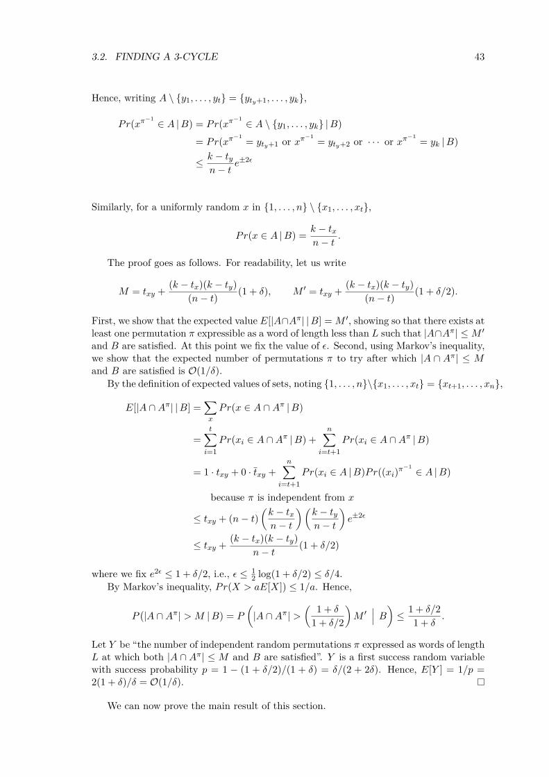
3.2. FINDING A 3-CYCLE 43
Hence, writing A \ {y1, . . . , yt} = {yty+1, . . . , yk},
Pr(xπ−1 ∈ A |B) = Pr(xπ−1 ∈ A \ {y1, . . . , yk} |B)
= Pr(xπ−1 = yty+1 or xπ−1 = yty+2 or · · · or xπ−1 = yk |B)
≤ k − tyn− t
e±2ε
Similarly, for a uniformly random x in {1, . . . , n} \ {x1, . . . , xt},
Pr(x ∈ A |B) = k − txn− t
.
The proof goes as follows. For readability, let us write
M = txy + (k − tx)(k − ty)(n− t) (1 + δ), M ′ = txy + (k − tx)(k − ty)
(n− t) (1 + δ/2).
First, we show that the expected value E[|A∩Aπ| |B] = M ′, showing so that there exists atleast one permutation π expressible as a word of length less than L such that |A∩Aπ| ≤M ′and B are satisfied. At this point we fix the value of ε. Second, using Markov’s inequality,we show that the expected number of permutations π to try after which |A ∩ Aπ| ≤ Mand B are satisfied is O(1/δ).
By the definition of expected values of sets, noting {1, . . . , n}\{x1, . . . , xt} = {xt+1, . . . , xn},
E[|A ∩Aπ| |B] =∑x
Pr(x ∈ A ∩Aπ |B)
=t∑i=1
Pr(xi ∈ A ∩Aπ |B) +n∑
i=t+1Pr(xi ∈ A ∩Aπ |B)
= 1 · txy + 0 · txy +n∑
i=t+1Pr(xi ∈ A |B)Pr((xi)π
−1 ∈ A |B)
because π is independent from x
≤ txy + (n− t)(k − txn− t
)(k − tyn− t
)e±2ε
≤ txy + (k − tx)(k − ty)n− t
(1 + δ/2)
where we fix e2ε ≤ 1 + δ/2, i.e., ε ≤ 12 log(1 + δ/2) ≤ δ/4.
By Markov’s inequality, Pr(X > aE[X]) ≤ 1/a. Hence,
P(|A ∩Aπ| > M |B) = P
(|A ∩Aπ| >
( 1 + δ
1 + δ/2
)M ′
∣∣∣ B) ≤ 1 + δ/21 + δ
.
Let Y be “the number of independent random permutations π expressed as words of lengthL at which both |A ∩ Aπ| ≤ M and B are satisfied”. Y is a first success random variablewith success probability p = 1 − (1 + δ/2)/(1 + δ) = δ/(2 + 2δ). Hence, E[Y ] = 1/p =2(1 + δ)/δ = O(1/δ).
We can now prove the main result of this section.

44 CHAPTER 3. FACTORIZING THE SYMMETRIC GROUP
Theorem 3.8 ([BBS04], variant of Theorem 1.1). If G = 〈S〉 = Sn or An, if S includesa permutation of degree less than n/4 and if n ≥ 39, then there exists a 3-cycle in Gexpressible as a word of length O(n6|S|(logn)O(1)) over S ∪ S−1, and such a word can befound in Las Vegas polynomial time.
Proof. The proof consists of the following algorithm.
1. Take τ a generator of degree less than n/4 in S.
2. Take x1, y1 ∈ supp(τ), x2 =6∈ supp(τ), y2 = (y1)τ , k = deg(τ) and
δ =((k − 7/2)(n− 2)
3(k − 1)(k − 2) − 1) /
2.
3. Try random permutations π as words of length O(n6|S| log(n) log(1/δ)) on S ∪ S−1
until (x1)π = y1, (x2)π = y2 and
| supp(τ) ∩ supp(τ)π| ≤ 1 + (k − 1)(k − 2)n− 2 (1 + δ).
4. Replace τ by [τ, τπ].
5. Repeat steps 2 to 4 until deg(τ) = 3.
Step 3 is an application of Lemma 3.7 with A = supp(τ), k = deg(τ), t = 2, txy = 1,tx = 1 and ty = 2. Since supp(τ)π = supp(τπ), by Proposition 1.44 and by the lemma,
deg([τ, τπ]) ≤ 3| supp(τ) ∩ supp(τπ)| = 3| supp(τ) ∩ supp(τ)π|
≤ 3 + 3(k − 1)(k − 2)n− 2 (1 + δ).
The choice of δ ensures that the degree of τ decreases strictly at each iteration. Indeed,
deg([τ, τπ]) ≤ 3 + 3(k − 1)(k − 2)n− 2 (1 + δ)
≤ 3 + 3(k − 1)(k − 2)n− 2 (1 + 2δ)
= 3 + 3(k − 1)(k − 2)n− 2
(k − 7/2)(n− 2)3(k − 1)(k − 2)
= k − 1/2 = deg(τ)− 1/2
Yet, Lemma 3.7 requires δ to be positive:((k − 7/2)(n− 2)3(k − 1)(k − 2) − 1
) /2 > 0
⇔ 3(k − 1)(k − 2) < (k − 7/2)(n− 2)⇔ 3k2 − (n+ 7)k + (7/2)n− 1 < 0
⇔ n+ 7−√n2 − 28 + 616 < k <
n+ 7 +√n2 − 28n+ 61
6 .
Hence, to be able to use the lemma for all k ∈ {4, . . . , n/4}, we must have
n+ 7−√n2 − 28n+ 61
6 < 4 and n/4 < n+ 7 +√n2 − 28n+ 61
6 ,

3.2. FINDING A 3-CYCLE 45
which respectively require n ≥ 39 and n ≥ 28. Hence, the algorithm requires n ≥ 39.By Proposition 3.6 and the choice of x1, x2, y1, y2 in step 2, [τ, τπ] 6= Id. Because a
commutator is an even permutation, [τ, τπ] can not be a 2-cycle. Hence, the algorithmconverges to a 3-cycle.
A brief study of δ shows that, for a given n: δ → −∞ as k → 2 and δ has only twolocal extrema: a local maximum at k = (7 −
√15)(n − 2)/2 and a local minimum at
k = (7 +√
15)(n−2)/2� n/4. Hence, for n fixed, the minimum value of δ on the interval[4, n/4] lays at one of its bounds: either
δ ≥((4− 7/2)(n− 2)
3(4− 1)(4− 2) − 1) /
2 = n/72− 19/36
or
δ ≥( (n/4− 7/2)(n− 2)
3(n/4− 1)(n/4− 2) − 1) /
2 = 1/6− 8(n+ 1)3(n− 8)(n− 4) .
Hence, for n ≥ 39,
δ ≥ min(n/72− 19/36, 1/6− 8(n+ 1)
3(n− 8)(n− 4)
)≥ min
(39/72− 19/36, 1/6− 8(39 + 1)
3(39− 8)(39− 4)
)= 1/72
Hence, in terms of complexity, the term O(1/δ) in step 3 is negligible.The complexity analysis goes as follows. Writing li the length of the word expressing
τ at the ith iteration and di its degree,
li+1 = 4li + 4K, l0 = 1
di+1 ≤ 3 + 3(di − 1)(di − 2)n− 2 (1 + δ)
≤ 3 + 3((di − 1)(di − 2)
n− 2
)(1/2 + (di − 7/2)(n− 2)
6(di − 1)(di − 2)
)= 3d2
i + (n− 11)di + 2(n+ 1)2(n− 2) , k0 ≤ n/4
where K = O(|S|n6 logn). One computes that
li = 4i + 43K(4i − 1) = O(4iK).
The study of di is more complicated. According to [BBS04], it reaches di = 3 at i =O(log logn).5 Since O(log logn) = O(1) log logn,
log(4O(log logn)) = log(4O(1) log logn) = O(1) · (log 4) · (log logn) = log((logn)O(1) log 4).5The exact claim in [BBS04] is: “if the degree of the old τ is k and the degree of the new τ is l then
l/n < 3/n + 3(k/n)2(1 + δ) for an arbitrary small δ. Since at start, k/n < 1/(3 + ε) for a fixed ε > 0, inO(log logn) rounds, we shall reach k = 3.” It has no further justification. We tried to prove it but we awall, as the recurrence equation xk+1 = ax2
k + bxk + c has no closed-form solution in general ([Wei]). Theclaim however seems sound: xk+1 = ax2
k has solution xk = (ax0)2k
/a2 and the few quadratic recurrenceequations in [Wei] that have a closed-form solution have a solution of type xk = α2k
. One may then guessthat the solution of any quadtratic recurrence equation grows at a rate of order (αx0)2k
, in which casexk = c would be reached at k = O(log log(x0)).

46 CHAPTER 3. FACTORIZING THE SYMMETRIC GROUP
Hence, 4O(log logn) = (logn)O(1) log 4 and the final length of τ is
O(4O(1) log lognn6|S| logn) = O((logn)O(1) log 4n6|S| logn) = O(n6|S|(logn)O(1)).
By Lemma 3.7, the permutations in steps 3 can be found in Las Vegas polynomialtime.
To close this section, here are the main differences between this section and [BBS04]:
• Lemma 2.2 in [BBS04]’s claims that there exists a word such that
|A ∩Aπ| ≤ txy + (k2/n)(1 + δ)
while we proved that
|A ∩Aπ| ≤ txy + (k − tx)(k − ty)n− t
(1 + δ).
This difference comes from a “calculation shortcut” in the original proof. At firstsight this seems harmless because the original bound looks like an overestimation ofour bound. In fact, however, the two bounds are incomparable: with tx = 1, ty = 2,txy = 1 and k = n/4 (the context of Theorem 3.8), the original bound is higher thanours for n ≥ 16/5 (which, in the context of Theorem 3.8, does not harm because weimpose n ≥ 39). But with some other choices, e.g., tx = ty = 0 and t = n/10, ourbound is always higher than the original one.Furthermore, if Theorem 3.8 uses the original bound, the convergence of the algo-rithm (i.e., deg([τ, τπ]) ≤ deg(τ)− 1/2) would require
δ ≤ (k − 7/2)n3k2 − 1
and that bound on δ would be positive only for
n−√n2 − 42n6 < k <
n+√n2 − 42n6
which, to be true for all k ∈ {4, . . . , n/4}, would require n ≥ 97. Hence, our boundensures the algorithm to work smaller groups than it would with the original bound.
• [BBS04] does not mention at which value the δ of the proof of 3.8 should be set.Hence, it does not mention that the algorithm does not converge for every δ andhence, it does not mention the “n ≥ 39” limitation which is a consequence of therestriction on δ for the algorithm to converge.
• We supply the proof of
deg([τ, τπ]) ≤ 3| supp(τ) ∩ supp(τπ)|,
in Proposition 1.44, which is omitted in [BBS04].
• Theorem 1.1 in [BBS04] claims that, when S contains a permutation of degree lessthan n/(3 + ε), the diameter of the Cayley graph Γ(G,S) is O(nC), but its proofshows how to find one 3-cycle, not mentioning the extra work needed once we findone 3-cycle (for instance, the results in [DF87]). We reproduce that work in the nextsection, giving the last step of the algorithm.

3.3. FACTORIZING ANY TARGET FROM A 3-CYCLE 47
3.3 Factorizing any Target from a 3-CycleIn this section we reproduce the following result from [DF87]: for a group G = 〈S〉 =Sn or An, if one can express a 3-cycle as a word of k generators, then one can factorizeany target of G as a word of at most kn+ n4 generators.
This comes from the combination of two results:
• if one has a 3-cycle as a word of k generators, then any other 3-cycle inG is expressibleas a word of at most k + n3 generators;
• any even permutation is expressible as a product of at most n 3-cycles.
Proposition 3.9 ([DF87], Lemma 2 with a modified claim). For any group G = 〈S〉 andH ≤ G, for every coset Hx, one can find an element x′ ∈ Hx expressible as a word oflength k ≤ [G : H] on S ∪ S−1.
Proof. Let Γ(G,S ∪ S−1, H) be the Schreier right coset graph (See Section 1.5). Thisgraph is unoriented, connected and has [G : H] vertices. Using a shortest path algorithmon graphs, for every x, one can find a path s1, s2, . . . , sk of length k ≤ [G : H] from H toHx. Equivalently, Hs1s2 · · · sk = Hx, or s1s2 · · · sk = x′ ∈ Hx.
Proposition 3.10 ([DF87], Theorem 5 with a modified claim). If G = 〈S〉 = Sn or An,n ≥ 5, has a 3-cycle expressible as a product of k generators, then every 3-cycle in G isexpressible as a product of at most k + n3 generators.
Proof. Let t be the k-expressible 3-cycle. By Corollaries 1.41 and 1.42, any other 3-cyclet′ in G is conjugate to t by some p: t′ = p−1tp.
Define H as the subgroup of G which fixes the support of t. In fact, t′ is conjugate tot by any element p′ = hp in the coset Hp: if h ∈ H, then h and t commute and
p′−1tp′ = (hp)−1t(hp) = p−1h−1thp = p−1h−1htp = ptp−1 = t′.
By the previous proposition, one can find a product s1s2 · · · sl = p′ ∈ Hp of lengthl ≤ [G : H] = n(n− 1)(n− 2)/3. Hence,
t′ = (s1s2 · · · sl)−1t(s1s2 · · · sl)
is a word of length at most k + 2n(n− 1)(n− 2)/3 ≤ k + n3.
Without loss of generality, one may assume that the target to factorize in G is even.If it is not, then G = Sn and S must have at least one odd generator. By multiplying thetarget by that generator, we now have an even target to factorize. The end of the problemis straightforward: by applying the proof of Proposition 1.36, the target can be writtenas a product of at most n 3-cycles that all can be written as words of at most k + n3
generators.


Chapter 4
Solving Rubik’s Cube withNon-Standard Moves
Building upon what we saw in Chapters 1 to 3, we can now answer our main question:how do we solve Rubik’s cube, given an arbitrary generating set?
Intuitively, the way our algorithm works is very similar to the strategy we presentedto solve the cube using the standard generators in Section 2.3: first we position the cubitsright, then we reorient them. Mathematically, Section 2.3 showed that
G ∼= N oH
where N = Z73 × Z11
2 corresponds to the orientations of the cubits, while H = {(p, q) ∈S8 × S12 | sgn(p) = sgn(q)} corresponds to the positioning of the cubits.
This chapter is divided into 3 sections:
• Section 4.1 adapts the algorithm of Chapter 3 to small permutation groups, especiallyA8 and A12;
• Section 4.2 uses the algorithm of Section 4.1 to factorize A8 ×A12;
• Section 4.3 uses the algorithm for A8 × A12 to build the algorithm that solves thecube.
This chapter is the counterweight of Chapter 3: if Chapter 3 focused on proving lemmasand theorems, this chapter is centered on the algorithm that solves the cube. We did notattempt to prove the complexity of our algorithm. Instead, we ran some tests to measurethe average and maximal word length one may expect from it.
4.1 Factorizing Small Groups
The algorithm we studied in Chapter 3 cannot be used as is to solve Rubik’s cube. Indeed,
• the first part of the algorithm, finding a permutation of degree less than n/4, merely“almost always” works (that means: the probability that it works tends to 1 asn→∞);
• the central part of the algorithm, reducing a permutation of degree less than n/4 toa 3-cycle, only works for n ≥ 39.
49

50 CHAPTER 4. SOLVING RUBIK’S CUBE WITH NON-STANDARD MOVES
5 10 20 300
0.25
0.75
1
n
fraction
An
Sn
An
Sn or
0.24
0.72
0.96
Figure 4.1: Fraction of pairs of permutations in Sn that generate Sn or An. One observesNetto’s conjecture: almost all pairs of permutations generate Sn or An.
To understand how much an almost always true proposition may be irrelevant forpractical purposes, let us take Dixon’s proof of Netto’s conjecture: almost all pairs ofpermutations in Sn generate either Sn or An. What Dixon exactly proved is:
Theorem 4.1 ([Dix69], Theorem 1). The proportion of ordered pairs (x, y) (x, y ∈ Sn)which generates either Sn or An is greater than
1− 2/(log logn)2
for all sufficiently large n.
The problem is that his bound grows extremely slowly and is even negative for n ≤ 61.Looking at the proof of his theorem, one sees that he proves a slightly higher bound,
1− (2/n)− 16/(3 log logn)2,
but even this bound is negative for n ≤ 50. Statements that are proven to “almost alway”work are hence to take with a pinch of salt when we are using them for practical purposes.
With some computer help (see Code A.7) however, we see that things are not that bad:44% of the ordered pairs generate S6. Due to the factorial number of elements in Sn, bruteforce calculation is not realistic: it takes Magma 44 seconds to perform the calculation forS6 and more than 10 minutes for S7, and the execution time should grow at least as fastas (n!)2, depending on how fast Magma compares two permutation groups. Finding allthe generators of Sn would then require about 10 hours for n = 8 and 36 days for n = 9.For that reason, for n ≥ 8, the calculation is done by taking 10 000 random couples in Snand counting how many do generate the full group. Launching the calculation on S30, weobserve that about 96% of the ordered couples in Sn generate either Sn or An, confirmingNetto’s conjecture (see Figure 4.1). Working with generating sets of two elements andtheir inverses is hence realistic, even for small symmetric groups.
If Babai et al.’s algorithm is not directly usable, we can adapt it to our case. As areminder, it first tries permutations στ i for some i’s until it finds a permutation that hasa cycle of length j ≥ 3n/4. Then, it rises that στ i to the jth power, which has the effectof “killing” the cycle of length j, such that τ ′ = (στ i)j is a permutation of degree less thann/4. Then, it iteratively replaces τ ′ by [τ ′, τ ′π] for some appropriate random permutationsπ to reduce the degree of τ ′ to 3. At this point, τ ′ is a 3-cycle. By conjugating τ ′, thealgorithm finds all the 3-cycles in Sn and expresses the target to factorize as a product of3-cycle (and, possibly, an odd generator).

4.2. FACTORIZING A8 ×A12 51
The main problem of the algorithm is that the second part, reducing τ ′ to a 3-cycle,has no guarantee to converge if n ≤ 38. This is however not a big problem for smallpermutation groups: indeed, for n ≤ 15, a permutation of degree less than n/4 is a 3-cycle(or a 2-cycle, which works fine too). For small groups, we can then skip the central partof the algorithm.
Here is hence our algorithm, inspired of Babai et al.’s work. Instead of looking for apermutation στ i with a cycle of length bigger than 3n/4, we do a breadth-first search onthe Cayley graph related to S (i.e., we explore the set of possible words on S) until wefind a permutation which can lead to a 3-cycle (resp 2-cycle) by rising it to an appropriatepower. Those permutations are easy to recognize: their cycle structure contains exactlyone 3-cycle (resp. 2-cycle) and has no other cycle with a length multiple of 3 (resp. multipleof 2). These “good” cycle structures are listed by Code A.8.
Once we get that 2- or 3-cycle, our algorithm ends by reusing Driscoll and Furst’sresults of Section 3.3: we find all the 3-cycles in Sn (or the 2-cycles) by conjugating thefound 3-cycle (or the 2-cycle), then we express the element to factorize as a product of3-cycles and possibly an odd generator (or as a product of 2-cycles).
The whole algorithm is implemented in Code A.11, requiring Codes A.8, A.10, A.4and A.5.
Does it work? To test our algorithm, we launched it on 10 000 random pairs of elementsin Sn generating the whole group, chosed a random target for these generating sets andrecorded the average and maximal word length it outputs. We repeated that experiencefor every n ∈ {5, 6, . . . , 30}. Quite unsurprising, the average word length of our algorithmseems to follow e(1/2+o(1)) log2 n (the average order of a permutation in Sn) and the maximalword length seems to follow e
√n logn (the maximal order of a permutation in Sn) (see
Figure 4.2). Indeed, the power to which we rise our permutation when we find our 3-cycle(resp. 2-cycle) corresponds to the order of that permutation divided by 3 (resp. by 2). Ifour algorithm works fine for small groups, it seems pretty uneffective for larger groups.
Specific tests on A8 and A12 (the groups we are interested in) gave an average andmaximal word length of 50.26 and 144 for A8, and 161.55 and 490 for A12.
4.2 Factorizing A8 × A12
Building upon the algorithm of the previous section, in this section we present an algorithmthat factorizes A8 ×A12. It is easily generalized to factorize any direct product Sn × Sm.
The idea is to first factor one term of the direct product, and then the other term.Given a generating set
S = {s1, . . . , sk} = {(s8,1, s12,1), . . . , (s8,k, s12,k)}
in S8×S12 that generates A8×A12 and a target t = (t8, t12), we start by factorizing t8 asa word on the generating set {s8,1, . . . , s8,k}. We then end up with a product
l∏j=1
sij =l∏
j=1(s8,ij , s12,ij ) = (t8, t′12)
for some t′12 in A12. The next step is to find a word on S that expresses the permutation(Id, t′−1
12 t12). Appending that word to the one expressing t8 will give us a word expressing(t8, t′12) · (Id, t′−1
12 t12) = (t8, t12).To find that second word, we reuse the idea from the previous section: we do a breadth-
first search on the Cayley graph related to S until we find a permutation that can be rised to

52 CHAPTER 4. SOLVING RUBIK’S CUBE WITH NON-STANDARD MOVES
5 10 20 300
14.7x 10
4
n
46
147684
maxword
length
5 10 20 300
1.66
5.17
log10(exp(√
n logn))
n
log 1
0(maxword
length)
5 10 20 300
5000
n
18.37
5378.58
avgword
length
5 10 20 300
1.26
3.73
log10(exp((1/2) log2 n))
n
log 1
0(avgword
length)
Figure 4.2: The average and maximal length of the words produced bysmallGroupFactorization for 10 000 random generating pairs of Sn and random elementsto factorize. The logarithm curve of these lengths suggest that our algorithm’s averagecomplexity is O(e(1/2) log2 n) (the average order of a permuatation in Sn) and maximalcomplexity is O(e
√n logn) (the maximal order of a permutation in Sn).
one of the form p = (Id, (a, b, c)) by rising it to an appropriate power. (Those permutationsare the permutations of the form (p8, p12) where p8 has no cycle of length multiple of 3and p12 has exactly one cycle of length 3 and no other cycle of length multiple of 3.) Oncewe have that permutation p, by conjugation we find all the 3-cycles in A12 and we end thealgorithm by expressing t′−1
12 t12 as a product of 3-cycles.The full algorithm is implemented in Code A.12 and reuses some codes that were
already written for the factorization of Sn. Tests on 10 000 random couples of permutationsgenerating A8 × A12 and random targets gave us an average and maximal word lengthproduced by the algorithm of 612.26 and 3103. These are roughly one order of magnitudehigher than the results we got to factorize A8 and A12 separately. The explanation behindthis order of magnitude is that the power at which one must rise the permutation foundby the breadth-first search to get a permutation of type (Id, (a, b, c)) is higher than thepowers to rise a permutation to a 3-cycle in A8 and A12. For A8 and A12, the worst powersare 5 and 7, while the worst power in A8 ×A12 is 70.
4.3 Solving Rubik’s Cube with Non-Standard Moves
Now that we have an algorithm to factorize A8×A12, we have everything in our hands topresent our algorithm that solves the cube.
As we saw in Chapter 2, Rubik’s group G ∼= N oφ H is a semi-direct product. Theway we factorize that semi-direct product is very similar to our algorithm for A8 × A12:

4.3. SOLVING RUBIK’S CUBE WITH NON-STANDARD MOVES 53
given a generating set S = {s1, . . . , sk} = {(s1,n, s1,h), . . . , (sk,n, sk,h)} and a target t =(tn, th) ∈ N oH,
• first we express th in terms of {s1,h, . . . , sk,h}: we then find a product
l∏j=1
sij = (t′n, th);
• second, we need to express (tnt′−1n , Id) in terms of S. By prepending this word to
the word expressing (t′n, th), we find a word expressing
(tnt′−1n , Id) · (t′n, th) = ((tnt′−1
n ) · t′nφ(Id), Id ·th) = (tn, th).
Concretely, take S = {s1, . . . , sk} a generating set ofG and take t ∈ G. Remember that,as presented in Section 2.1, πc(t) ∈ S8 corresponds to the positioning of the corner cubits,πs(t) ∈ S12 corresponds to the positioning of the side cubits, ρc(t) ∈ Z8
3 corresponds to theorientation of the corner cubits, and ρs(t) ∈ Z12
2 corresponds to the orientation of the sidecubits. Write pc = πc(t), ps = πs(t), rc = ρc(t) and rs = ρs(t). The main result of Chap-ter 2 is that G ∼= NoH where H ∼= {(p, q) ∈ S8×S12 | sgn(p) = sgn(q)} and N ∼= Z7
3×Z112 .
Since πc and πs are homomorphisms, S{H} = {(πc(s1), πs(s1)), . . . , (πc(sk), πs(sk))} is agenerating set of H. (Note that {(ρc(s1), ρs(s1)), . . . , (ρc(sk), ρs(sk))} does not necessarilyform a generating set of N .)
The first step is to factorize (pc, ps) ∈ H. If pc is even, we can directly use the algorithmwe developed for A8×A12. Else, we must first multiply t by a generator s such that πc(s)is odd. (Such a generator must exist.) We then get a first word w1 on S expressing apermutation t′ such that
t′ =l∏
j=1sij
πc(t′) = pc πs(t′) = ps ρc(t′) = r′c ρs(t′) = r′s
where potentially r′c 6= rc and r′s 6= rs.The second step is to factorize t1 such that
πc(t1) = πs(t1) = Id ρc(t1) = rc − r′c ρs(t1) = rs − r′s.
For this purpose, we need 7 moves mi and 11 moves nj such that
πc(mi) = πs(mi) = πc(nj) = πs(nj) = Id for every i and j,
and such that {ρc(mi)} and {ρs(nj)} are linearly independent sets. We find these moveswith the following algorithm:
1. start with two empty sets M and N and two empty word sets WM and WN ;
2. take a uniformly random word w on S and denote h ∈ G its corresponding permu-tation. We choose w to have a length 40, because it equals two times God’s number,the diameter of the Cayley graph of G with the standard generators;
3. factorize (πc(h), πs(h)) ∈ S8 × S12 as a word w′ using last chapter’s algorithm;

54 CHAPTER 4. SOLVING RUBIK’S CUBE WITH NON-STANDARD MOVES
4. write w′′ = w−1w′ the concatenation of w−1 (the word expressing h−1 and w′, andh′′ its corresponding permutation. By construction, πc(h′′) = πs(h′′) = Id;
5. if ρc(h′′) is linearly independent to the elements in M , add h′′ to M and w′′ to WM ;
6. if ρs(h′′) is linearly independent to the elements in N , add h′′ to N and w′′ to WN ;
7. repeat steps 2 to 5 until M has 7 elements and N has 11 elements.
From here, we express rs − r′s as a linear combination of {ρs(nj)} and take the corre-sponding words in WN to get a word w2 on S expressing a permutation t′′ such that
πc(t′′) = ρc(t′′) = Id ρc(t′′) = r′′c ρs(t′′) = rs − r′s
where potentially r′′c 6= rc − r′c. The last step is to express rc − r′c − r′′c in terms of{mi}. However, since potentially ρc(mi) 6= 0, we express it in terms of {m2
i }. Indeed,ρc(m2
i ) = 2ρc(mi) = −ρc(mi) and ρs(m2i ) = 2ρs(mi) = 0. We then get a third word w3.
Concatenating w3, w2 and w1, we get a word expressing t on S.From the cube’s perspective, the first word w1 corresponds to a move that positions the
corner and side cubits in their correct cubicles. Remind that the algorithm that factorizesA8 × A12 first factorizes A8 independently of A12 and then factorizes A12 using elementsthat do not undo the work done on A8. The first step consists hence of first setting thecorner cubits at their correct place independently of the side cubits, and then places theside cubits right using moves that do not reposition the corner cubits. The second stepworks by using moves that reorient the cubits without repositioning them. First, the wordw2 reorient the side cubits independently of the corner cubits, then the word w3 reorientsthe corner cubits using moves that do not reorient the correctly oriented side cubits. Thissolution of the cube is hence very similar to the one we presented in Section 2.3.
The full algorithm is implemented in Code A.13. On the standard generating set, for1000 random elements t ∈ G, it produces words of average and maximal length 3707.48and 6211, compared to the maximum of 1435 for the algorithm we gave in Section 2.3. For1000 random pairs of elements in G and random elements t ∈ G, the algorithm produceswords of average and maximal length 13 573.94 and 78 588.
One may be skeptical about our algorithm and say that there is no guarantee that wewill find the elements {mi} and {nj} in a “reasonable” time. Our experiments suggest theopposite. On the 1000 random couples of elements generating G, it takes in average 7.67and 12.53 random elements h to find the 7 and 11 linearly independent vectors ρc(mi)and ρs(nj). (That is, almost every random word taken leads to a vector that is linearlyindependent to the previously found ones.)

Conclusion and Further Work
Let us recap what has been done in this thesis: Chapter 1 provided us the notions requiredin group theory; Chapter 2 presented the group structure behind Rubik’s cube and a way tosolve it with the standard generators; Chapter 3 presented Babai et al.’s work to factorizeSn in polynomial time when n ≥ 39; Chapter 4 adapted the algorithm from Chapter 3 towork for smaller groups and used it as a brick to solve Rubik’s cube for any generatingset. Both solutions presented in Chapters 2 and 4 follow the same systematic approach:first position the cubits at their right place regardless of their orientations, then reorientthem right by using moves that have no effect on the positioning of the cubits.
Through Rubik’s cube, we studied the factorization of a semi-direct product includingsmall permutation groups. The most straightforward next step would be to extend ouralgorithm to solve Rubik’s n × n × n cube, which should have a similar group structure.One may also want prove a clean bound on the complexity of our algorithm, rather thanrelying on tests to study its performance. Last, one may want to improve our algorithmso that it solves the cube with shorter words.
55


Bibliography
[Ban82] C. Bandelow, Inside rubik’s cube and beyond, Birkhäuser, 1982.
[BBS04] László Babai, Robert Beals, and Ákos Seress, On the diameter of the symmetricgroup: Polynomial bounds, Proceedings of the Fifteenth Annual ACM-SIAMSymposium on Discrete Algorithms (Philadelphia, PA, USA), SODA ’04, So-ciety for Industrial and Applied Mathematics, 2004, pp. 1108–1112.
[BH05] László Babai and Thomas P. Hayes, Near-independence of permutations and analmost sure polynomial bound on the diameter of the symmetric group, Proceed-ings of the Sixteenth Annual ACM-SIAM Symposium on Discrete Algorithms(Philadelphia, PA, USA), SODA ’05, Society for Industrial and Applied Math-ematics, 2005, pp. 1057–1066.
[BHH+10] Olof Bergvall, Elin Hynning, Mikael Hedberg, Joel Mickelin, and Patrick Ma-sawe, On rubik’s cube, Bachelor’s thesis, Kungliga Tekniska Högskolan, Stock-holm, May 2010.
[BS88] László Babai and Ákos Seress, On the diameter of cayley graphs of the sym-metric group., J. Comb. Theory, Ser. A 49 (1988), no. 1, 175–179.
[Che78] Janet Chen, Group theory and the rubiks cube, 1978, available on www.math.harvard.edu/~jjchen/, accessed 7 Jul 2014.
[DF87] James R. Driscoll and Merrick L. Furst, Computing short generator sequences,Inf. Comput. 72 (1987), no. 2, 117–132.
[DF04] David Steven Dummit and Richard M. Foote, Abstract algebra, John Wiley &sons, Hoboken, NJ, 2004.
[Dix69] John D. Dixon, The probability of generating the symmetric group, Math. Z.110 (1969), 199–205. MR 40 #4985
[EG81] Shimon Even and Oded Goldreich, The minimum-length generator sequenceproblem is np-hard., J. Algorithms 2 (1981), no. 3, 311–313.
[ET65] Pál Erdős and Pál Turán, On some problems of a statistical group-theory. I.,Z. Wahrscheinlichkeitstheor. Verw. Geb. 4 (1965), 175–186 (English).
[HSZ14] Harald A. Helfgott, Ákos Seress, and Andrzej Zuk, Random generators of thesymmetric group: diameter, mixing time and spectral gap, 2014, available onhttp://arxiv.org/abs/1311.6742, accessed 7 Jul 2014.
[Isa12] Carl Joakim Isaksen, Rubik’s cube and group theory, Master’s thesis, Universityof Oslo, June 2012.
57

58 BIBLIOGRAPHY
[Jer85] Mark R. Jerrum, The complexity of finding minimum-length generator se-quences, Theoretical Computer Science 36 (1985), no. 0, 265 – 289.
[LO81] H. J. Landau and A. M. Odlyzko, Bounds for eigenvalues of certain stochasticmatrices, j-LINEAR-ALGEBRA-APPL 38 (1981), 5–15. MR 82m:15022
[Mil87] William Miller, The maximum order of an element of a finite symmetric group,Am. Math. Monthly 94 (1987), no. 6, 497–506.
[PQ11] Christophe Petit and Jean-Jacques Quisquater, Rubik’s for cryptographers.,IACR Cryptology ePrint Archive 2011 (2011), 638.
[Wei] Eric W. Weisstein, Quadratic map—mathworld, a wolfram web resource, online,available on http://mathworld.wolfram.com/QuadraticMap.html, accessed11 May 2014.

Appendix A
Code Snippets
Each code snippet consists of a file myFunction.mag describing a function myFunction.Some functions are built upon other ones and load thme through the instruction load"theFunction.mag"; in their corresponding files. Hence, for everything to work well, allthe files need to be placed in a same folder.
A.1 Rubik’s Cube
Listing A.1: rubik.mag// rubik.mag// Author: Laurent Van Eesbeeck// Date: 2014-08-19
S:=Sym(48);
// positionings and orientationsV2:=VectorSpace(FiniteField(2),12); // Z_2^12V3:=VectorSpace(FiniteField(3),8); // Z_3^8pic:=func< m | Sym(8) ! [Ceiling( (3*i)^m / 3) : i in [1..8]]>;pis:=func< m | Sym(12) ! [Ceiling( (24+2*i)^m / 2)-12 : i in [1..12]]>;rhoc:=func< m | V3![(3*i)^m mod 3 : i in [1..8]]>;rhos:=func< m | V2![(24+2*i)^m mod 2 : i in [1..12]]>;
// the inverse functioninv:=func<pc,ps,rc,rs |Sym(48)! ( &cat[[3*(i^pc) - IntegerRing()!(-rc[i]+j) : j
in [2,1,0]] : i in [1..8]]cat &cat[[2*(i^ps)+24 - IntegerRing()!(-rs[i]+j) : j in [1,0]] : i in
[1..12]])>;
// the Rubik’s groupU:=S!(1, 10, 7, 4)(2, 11, 8, 5)(3, 12, 9, 6)(25, 31, 29, 27)(26, 32, 30, 28);D:=S!(13, 16, 19, 22)(14, 17, 20, 23)(15, 18, 21, 24)(41, 43, 45, 47)(42, 44, 46,
48);L:=S!(4, 9, 19, 18)(5, 7, 20, 16)(6, 8, 21, 17)(27, 38, 43, 36)(28, 37, 44, 35);R:=S!(1, 14, 22, 11)(2, 15, 23, 12)(3, 13, 24, 10)(31, 34, 47, 40)(32, 33, 48,
39);F:=S!(1, 6, 16, 15)(2, 4, 17, 13)(3, 5, 18, 14)(25, 35, 41, 33)(26, 36, 42, 34);B:=S!(7, 12, 22, 21)(8, 10, 23, 19)(9, 11, 24, 20)(29, 39, 45, 37)(30, 40, 46,
38);
59

60 APPENDIX A. CODE SNIPPETS
Moves:=[U,D,L,R,F,B];G:= sub<S|Moves>;
// // a random element to test that the functions are correct// g:=Random(G); g;// "";// pc := pic(g); pc;// ps := pis(g); ps;// rs := rhos(g); rs;// rc := rhoc(g); rc;// "";// g eq inv(pc,ps,rc,rs); // should return true
A.2 Babai et al’s factorization of Sn
Listing A.2: findDegreeLessThanN4.mag// findDegreeLessThanN4.mag// Author: Laurent Van Eesbeeck// Date: 2014-08-19
function findDegreeLessThanN4(S)// given a generating set S of Sn or An, returns a permutation p// of degree less than n/4 and a word w expressing it:// &*[S[w[i]] : i in [1..#w]] equals p// Observe that this function is only proved to ‘‘almost always’’ work.// When it does not, it returns the identity and an empty word.// return: p, w
n:=Degree(Parent(S[1]));id:=Id(Sym(n));
s:=S[1];if S[2] ne s^-1 then
t:=S[2]; x:=2;else
t:=S[3]; x:=3;end if;i:=1;
while not ((Degree(t) le n/4)or ( (CycleStructure(s*t)[1][1] ge 3*n/4)
and ((s*t)^CycleStructure(s*t)[1][1] ne Id(Sym(n))) )) dot:=t*S[x];i:=i+1;
end while;j:=0;
if t eq Id(Sym(n)) thenreturn id, [];
elif CycleStructure(s*t)[1][1] ge 3*n/4 thenp:=s*t;

A.2. BABAI ET AL’S FACTORIZATION OF SN 61
j:=CycleStructure(p)[1][1];p:=p^j;w:=&cat[
[1] cat [x : k in [1..i]]: l in [1..j]];
elsep:=t;w:=[x : k in [1..i]];
end if;return p,w;
end function;
Listing A.3: find3Cycle.mag// find3Cycle.mag// Author: Laurent Van Eesbeeck// Date: 2014-08-19
function find3Cycle(S,p)// Given S generating either Sn or An and a permutation p of degree// less than n/4, returns a 3-cycle t in Sn and a word expressing it:// &*[S[w[i]] : i in [1..#w]] equals t.// Note that since p may not belong to S, the occurrences of p and p^-1// in w are represented by the letters #S+1 and #S+2.// This function needs S to include its inverses. If it does not,// an empty word is returned instead// returns: t, w
n:=Degree(Parent(S[1]));id:=Id(Sym(n));SWithP:=S cat [p,p^-1];t:=p;w:=[#S+1]; // the initial word expressing t
// S[i]^-1 = S[invMap[i]]invMap:=[ Index(SWithP,s^-1) : s in SWithP ];if 0 in invMap then // case where S does not include its inverses
"Error in find3Cycle:";" the generating set does not include the inverses of its elements.";" Null word returned.";return [];
end if;// if w is a word expressing p, invWord(w) expresses p^-1invWord:= func< w | [ invMap[w[i]] : i in [#w..1 by -1] ] >;
M:=3*(#S)*Ceiling(Log(n))*n^6;tmp:=[0]; tmp[10]:=0;while Degree(t) gt 3 do
k:=Degree(t);delta:=( (k-7/2)*(n-2) / (3*(k-1)*(k-2)) -1 )/2;
r:=Random({1..#S});i:=1; p:=S[r]; tmp[i]:=r;

62 APPENDIX A. CODE SNIPPETS
while((#(Support(t) meet Support(t)^p) gt 1+(k-1)*(k-2)*(1+delta)/(n-2))or ((t,t^p) eq id) )and (i lt M) do// do this to allocate the memory progressivelyif i eq #tmp then tmp[Min([2*i,M])]:=0; end if;r:=Random({1..#S});i:=i+1; p:=p*S[r]; tmp[i]:=r;
end while;
if i lt M then // case where a permutation pi has been foundt:=(t,t^p);// w2 is the word expressing t^pw2:= invWord([tmp[j] : j in [1..i]]) cat w cat [tmp[j] : j in [1..i
]];w:=invWord(w) cat invWord(w2) cat w cat w2;
end if;end while;
return t,w;end function;
Listing A.4: findAllKCycles.mag// findAllKCycles.mag// Author: Laurent Van Eesbeeck// Date: 2014-08-19
function findAllKCycles(c,S)// given a k-cycle c in Sn, returns the lists// - kCycles which contains every k-cycle in <S>// - words which is a list of words on S expressing permutations:// perms[i] = &*[S[j] : j in words[i]]// where the ith k-cycle kCycles[i] is the conjugate of c by perms[i]:// kCycles[i] = c^(perms[i])// This function assumes that all k-cycles are conjugate in the group// generated by S.
// pre-allocation: there are nk=n!/(k! * k) k-cycles in Snn:=Degree(Parent(S[1]));k:=Degree(c);nk:=Factorial(n)/(Factorial(n-k) * k);nk:=IntegerRing()!nk;kCycles:=[c]; kCycles[nk]:=c;perms:=[Sym(n)!1]; perms[nk]:=Sym(n)!1;words:=[[]]; words[nk]:=[];
// this function uses /a lot/ of membership testings to a sequence// of nk elements. To make these testings more effective,// we use a hash table and a specific hash function for k-cycleshashTable:=[false : i in [1..(&+[n^i : i in [1..k]])]];function cycleHash(c)
// for the k-cycle (c1, ..., ck), returns the integer// c1 + c2*n + ... + ck*n^(k-1) which is unique to that k-cycle.x:=Min(Support(c));
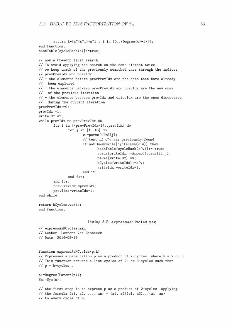
A.2. BABAI ET AL’S FACTORIZATION OF SN 63
return &+[x^(c^i)*n^i : i in [0..(Degree(c)-1)]];end function;hashTable[cycleHash(c)]:=true;
// now a breadth-first search.// To avoid applying the search on the same element twice,// we keep track of the previously searched ones through the indices// prevPrevIdx and prevIdx:// - the elements before prevPrevIdx are the ones that have already// been explored// - the elements between prevPrevIdx and prevIdx are the new ones// of the previous iteration// - the elements between prevIdx and writeIdx are the ones discovered// during the current iterationprevPrevIdx:=0;prevIdx:=1;writeIdx:=2;while prevIdx ne prevPrevIdx do
for i in [(prevPrevIdx+1)..prevIdx] dofor j in [1..#S] do
w:=perms[i]*S[j];// test if c^w was previously foundif not hashTable[cycleHash(c^w)] then
hashTable[cycleHash(c^w)]:= true;words[writeIdx]:=Append(words[i],j);perms[writeIdx]:=w;kCycles[writeIdx]:=c^w;writeIdx:=writeIdx+1;
end if;end for;
end for;prevPrevIdx:=prevIdx;prevIdx:=writeIdx-1;
end while;
return kCycles,words;end function;
Listing A.5: expressAsKCycles.mag// expressAsKCycles.mag// Author: Laurent Van Eesbeeck// Date: 2014-08-19
function expressAsKCycles(p,k)// Expresses a permutation p as a product of k-cycles, where k = 2 or 3.// This function returns a list cycles of 2- or 3-cycles such that// p = &*cycles .
n:=Degree(Parent(p));Sn:=Sym(n);
// the first step is to express p as a product of 2-cycles, applying// the formula (a1, a2, ..., an) = (a1, a2)(a1, a3)...(a1, an)// to every cycle of p.

64 APPENDIX A. CODE SNIPPETS
supportToCheck:=Support(p);cycles:=[]; i:=1;while supportToCheck ne {} do
c1:=Min(supportToCheck); x:=c1;Exclude(~supportToCheck,x);while x^p ne c1 do
x:=x^p;Exclude(~supportToCheck,x);cycles[i]:=Sn!(c1,x);i:=i+1;
end while;end while;
// The second step, if k = 3, is to apply the formula// (a,b)(a,b) = Id// (a,b)(a,c) = (a,b,c)// (a,b)(c,d) = (a,b,d)(a,c,d)// pairwise to the chain of 2-cyclesif k eq 3 then
function Convert2To3Cycles(c1,c2)c:=c1*c2;if Degree(c) eq 3 then
return [c];elif Degree(c) eq 4 then
s1:=[x : x in Support(c1)];s2:=[x : x in Support(c2)];return [Sn!(s1[1],s1[2],s2[2]), Sn!(s1[1],s2[1],s2[2])];
elsereturn [];
end if;end function;cycles:=&cat[Convert2To3Cycles(cycles[i],cycles[i+1]) : i in [1..#cycles
by 2]];end if;return cycles;end function;
Listing A.6: babaisFactorization.mag// babaisFactorization.mag// Author: Laurent Van Eesbeeck// Date: 2014-08-19
load "findDegreeLessThanN4.mag";load "find3Cycle.mag";load "findAllKCycles.mag";load "expressAsKCycles.mag";
function babaisFactorization(S,g)// given a set S generating either Sn or An and an element g in that group,// returns a word expressing g on S. S is supposed to include the inverses// of the generators too.// Note that, depending on S, the algorithm ‘‘almost always’’ works.// In case of failure, the algorithm returns an empty word.// Output: a sequence w such that

A.2. BABAI ET AL’S FACTORIZATION OF SN 65
// &*[ S[w[i]] : i in [1..#w]] equals g
n:=Degree(Parent(S[1]));Sn:=Sym(n);id:=Id(Sn);
// First, find a permutation of degree less than n/4pn4,wn4:=findDegreeLessThanN4(S);if pn4 eq id then // the algorithm failed
"Bad luck in babaisFactorization:";" no permutation with degree less than n/4 found.";" Try with other generators.";" Empty word returned.";return [];
end if;
// If pn4 is not a 2- or a 3-cycle, make a 3-cycle out of it// Notice that find3Cycle uses an extended generating set,// S cat [pn4, pn4^-1], hence the word w3 it outputs will have to be// translatedif Degree(pn4) gt 3 then
c3,w3:=find3Cycle(S,pn4);else
c3:=pn4; w3:=wn4;end if;
// Now find all the 3-cycles (or 2-cycles) based on c3cycles,cycleWords:=findAllKCycles(c3,S);
// And finally, express g as a product of 3-cycles (or 2-cycles)// (Note that if g is odd and c3 is a 3-cycle, we must first multiply// g by an odd generator)postMultiplyG:=false;if IsOdd(g) and Degree(c3) eq 3 then
postMultiplyG:=true;oddGenIdx:=Min( [ i : i in [1..#S] | IsOdd(S[i]) ] );g:=g*S[oddGenIdx];
end if;cyclesOfG:=expressAsKCycles(g,Degree(c3));
// Now the remaining work is to put all these parts together and build// the word expressing g out of it:// we must express every k-cycle in cyclesOfG correctly...invMap:=[ Index(S,s^-1) : s in S ];// if w is a word expressing p, invWord(w) expresses p^-1invWord:= func< w | [ invMap[w[i]] : i in [#w..1 by -1] ] >;if 0 in invMap then // case where S does not include its inverses
"Error in smallGroupFactorization:";" the generating set does not include the inverses of its elements.";" Null word returned.";return [];
end if;
word:=&cat[invWord(cycleWords[Position(cycles,c)]) cat w3 cat cycleWords[Position(
cycles,c)]

66 APPENDIX A. CODE SNIPPETS
: c in cyclesOfG];
// and we must replace the occurrences of #S+1 and #S+2 in w3 by// wn4 and invWord(wn4)function translatePN4(l)
if l le #S then return [l];elif l eq #S+1 then return wn4;elif l eq #S+2 then return invWord(wn4);else return [];end if;
end function;word:=&cat[translatePN4(l) : l in word];// last, we must consider the case where g was multiplied by an odd generatorif postMultiplyG then
word:= word cat [invMap[oddGenIdx]];end if;
return word;end function;
A.3 Small Groups
Listing A.7: countGenerators.mag// countGenerators.mag// Author: Laurent Van Eesbeeck// Date: 2014-08-19
function countGeneratorsOfSnAn(n,option)// counts the ratio of ordered pairs (x,y) in Sn that generate Sn or An// option = 0 -> counts for An// option = 1 -> counts for SnSn:=Sym(n); An:=Alt(n);
if option eq 0 then G:= An; else G:=Sn; end if;
// caution: the calculation takes about 15’ for n=7 and the execution time// seems to have a time complexity of O(n^2). Hence, for higher values of// n we count the generators amongst a set of 10 000 randomly chosen// couples of permutations.if n le 7 then
return #[[g,h] : g in Sn, h in Sn | sub<Sn|[g,h]> eq G]/(#Sn^2);else
randomCouples:=[[Random(Sn),Random(Sn)] : i in [1..10000]];return #[c : c in randomCouples | sub<Sn|[c[1],c[2]]> eq G]/#randomCouples
;end if;
end function;
Listing A.8: listGoodCycleStructures.mag// listGoodCycleStructures.mag// Author: Laurent Van Eesbeeck// Date: 2014-08-19

A.3. SMALL GROUPS 67
function listGoodCycleStructures(n,k,option)// lists all cycle structures in Sn that be rised to a k-cycle (k = 2 or 3)// The cycle structures are given in their Magma representation, i.e.,// (1,2,3)(4,5,6,7)(8)(9,10,11) in S_11 has as cycle structure the list// [<4,1>,<3,2>,<1,1>]// option = 0 -> cycle structures in A_n// option = 1 -> cycle structures in S_n//// note: listGoodCycleStructures(n,2,0) returns an empty sequence because// obviously, no permutation in A_n can be rised to a 2-cycle.
if (k eq 2) and (option eq 0) thenreturn {};
end if;
// A partition of n is a list [k1, ..., kj] such that k1 + ... + kj = n.// Partitions lists all the partitions of a given nC:= Partitions(n);
// now let us rewrite the partitions of n in Magma’s representation of// a cycle structure. This line transforms the partition of, say, n=5,// e.g., c:=[3,1,1], in the list [<5,0>, <4,0>, <3,1>, <2,0>, <1,2>]C:=[
[ < i, #[1: j in [1..#c] | c[j] eq i] > : i in [n..1 by -1] ]: c in C
];
// this line withdraw the elements of the form <k,0> from the listsC:=[
[ <c[i][1],c[i][2]> : i in [1..n] | c[i][2] ne 0 ]: c in C
];
// observe that even permutations must have an even number of even cycles// this small function spots odd cycle structures outfunction isEvenStructure(c)
for i in [1..#c] doif (c[i][1] mod 2 eq 0) and (c[i][2] mod 2 eq 1) then return false;
end if;end for;return true;
end function;
function goodForKCycle(c,k)if <k,1> notin c then return false; end if;
Exclude(~c,<k,1>);return &*[GCD(k,x[1]) : x in c] eq 1;
end function;
// now we filter the bad cycle structuresif option eq 0 then
C:={ c : c in C | isEvenStructure(c) };end if;

68 APPENDIX A. CODE SNIPPETS
if k eq 2 thenC:={ c : c in C | goodForKCycle(c,2)};
elif k eq 3 thenC:={ c : c in C | goodForKCycle(c,3)};
end if;
return C;end function;
Listing A.9: numberOfPermsPerCycleStructure.mag// numberOfPermsPerCycleStructure.mag// Author: Laurent Van Eesbeeck// Date: 2014-08-19
function numberOfPermsPerCycleStructure(c)// For c a cycle structure of form [<c1,i1>, <c2,i2>, ..., <ck,ik>],// the number of permutations in Sn following with c as cycle structure is// n! / ( (c1^i1 * c2^i2 * ... * ck^ik) * (i1! * i2! * ... * ik!) )
n:=&+[ x[1]*x[2] : x in c ];d:=&*[ x[1]^x[2] * Factorial(x[2]) : x in c ];return Factorial(n)/d;
end function;
Listing A.10: findPermutationWithGivenCycleStructure.mag// findPermutationWithGivenCycleStructure.mag// Author: Laurent Van Eesbeeck// Date: 2014-08-19
function findPermutationWithGivenCycleStructure(S,CS)// Given a generating set S of Sn, do a breadth-first search// until it finds a permutation p whose cycle structure is in CS.// The function also returns a word w on S expressing p.// output: p, w.
n:=Degree(Parent(S[1]));Sn:=Sym(n);perms:=[Id(Sn)];words:=[[]];foundPermutation:=false;kTested:=1;
// perms is a list of permutations already explored, which is divided in 2:// - the permutations that have already been multiplied with the generators// (index from 1 to kTested-1)// - the permutations that have not been multiplied with the generators// yet, with index from kTested to #permswhile not foundPermutation do
currNumberOfPerms:=#perms;for i in [kTested..#perms] do
for j in [1..#S] dop:=perms[i]*S[j];w:=Append(words[i],j);if p in perms then continue; end if;

A.3. SMALL GROUPS 69
if CycleStructure(p) in CS thenreturn p,w;
end if;words:=Append(words,w);perms:=Append(perms,p);
end for;end for;kTested:=currNumberOfPerms+1;
end while;
end function;
Listing A.11: smallGroupFactorization// smallGroupFactorization.mag// Author: Laurent Van Eesbeeck// Date: 2014-08-19
load "listGoodCycleStructures.mag";load "findPermutationWithGivenCycleStructure.mag";load "findAllKCycles.mag";load "expressAsKCycles.mag";
function smallGroupFactorization(S,g)// given a generating set S of Sn or An and an element g in that group,// returns a word on S expressing g:// &*[ S[w[i]] : i in [1..#w] ] equals g// Note that S must include its inverses too.
n:=Degree(Parent(S[1]));Sn:=Sym(n);// First we list the cycle structures we will be looking for.if sub<Sn|S> eq Sn then
option:=1;else
option:=0;end if;CycleStructuresFor2Cycles:=listGoodCycleStructures(n,2,option);CycleStructuresFor3Cycles:=listGoodCycleStructures(n,3,option);
// Then we find a permutation with one of the given cycle structures// and make a k-cycle out of it.goodP, goodWord :=findPermutationWithGivenCycleStructure(S,
CycleStructuresFor2Cycles join CycleStructuresFor3Cycles);CS:=CycleStructure(goodP);if CS in CycleStructuresFor2Cycles then
// goodP can be rised to a 2-cyclej:=LCM([CS[x][1] : x in [1..#CS]])/2;
else // goodP can be rised to a 3-cyclej:=LCM([CS[x][1] : x in [1..#CS]])/3;
end if;j:=IntegerRing()!j;kCycle:=goodP^j;kCycleWord:=&cat[ goodWord : i in [1..j] ];

70 APPENDIX A. CODE SNIPPETS
// from here, the code is very similar to Babai et al’s factorization.// Now find all the 3-cycles (or 2-cycles) based on kCyclecycles,cycleWords:=findAllKCycles(kCycle,S);
// And finally, we express g as a product of 3-cycles (or 2-cycles)// (Note that if g is odd and kCycle is a 3-cycle, we must first multiply// g by an odd generator)postMultiplyG:=false;if IsOdd(g) and Degree(kCycle) eq 3 then
postMultiplyG:=true;oddGenIdx:=Min( [ i : i in [1..#S] | IsOdd(S[i]) ] );g:=g*S[oddGenIdx];
end if;cyclesOfG:=expressAsKCycles(g,Degree(kCycle));
// Now the remaining work is to put all these parts together and build// the word expressing g out of it:// we must express every k-cycle in cyclesOfG correctlyinvMap:=[ Index(S,s^-1) : s in S ];if 0 in invMap then // case where S does not include its inverses
"Error in smallGroupFactorization:";" the generating set does not include the inverses of its elements.";" Null word returned.";return [];
end if;// if w is a word expressing p, invWord(w) expresses p^-1invWord:= func< w | [ invMap[w[i]] : i in [#w..1 by -1] ] >;word:=&cat[
invWord(cycleWords[Position(cycles,c)]) cat kCycleWord cat cycleWords[Position(cycles,c)]
: c in cyclesOfG];
// last, we must consider the case where g was multiplied by an odd generatorif postMultiplyG then
word:= word cat [invMap[oddGenIdx]];end if;
return word;end function;
Listing A.12: factorizeA8xA12.mag// factorizeA8xA12.mag// Author: Laurent Van Eesbeeck// Date: 2014-08-19
// The function builds upon smallGroupFactorizationload "smallGroupFactorization.mag";
function factorizeA8xA12(S,g)// given a generating set S of A8xA12 containing its inverses// and an element g=(g8,g12) in A8xA12, returns a word on S expressing g:// &*[ S[w[i]] : i in [1..#w] ] equals g.// The algorithm requires S to include the inverse of its elements.// S and g must be elements in DirectProduct(Sym(8),Sym(12))

A.3. SMALL GROUPS 71
S8S12:=DirectProduct(Sym(8),Sym(12));if g notin S8S12 or true in [s notin S8S12 : s in S] then
"Error in factorizeA8xA12:";" S or g is not in DirectProduct(Sym(8),Sym(12)).";" Empty word returned.";return [];
end if;
// Note: Magma treats direct products of symmetric groups as subgroups// of a bigger symmetric group. Given that A8 is generated by// (1,2,3) and (1,2)(3,4,5,6,7,8) and that A12 is generated by// (1,2,3) and (1,2)(3,4,5,6,7,8,9,10,11,12),// Magma considers A8xA12 as the subgroup of S20 generated by// (1,2,3), (1,2)(3,4,5,6,7,8), (9,10,11)// and (9,10)(11,12,13,14,15,16,17,18,19,20).// (the A8 part is covered by the elements 1..8 and the A12 part is covered// by the elements 9 to 20.)// To ease our manipulations, we need some functions to go back and forth// between S20, A8 and A12.
A8toA8A12 := func< p | Sym(20)! ([i^p : i in [1..8]] cat [9..20]) >;A12toA8A12:= func< p | Sym(20)! ([1..8] cat [i^p+8 : i in [1..12]]) >;A8A12toA8 := func< p | Sym(8)! [i^p : i in [1..8]] >;A8A12toA12:= func< p | Sym(12)! [i^p-8: i in [9..20]] >;
// Now we can start the algorithm.// The first step is to factorize the part in A8 using smallGroupFactorizationS8:=[A8A12toA8(s) : s in S];S12:=[A8A12toA12(s) : s in S];g8:=A8A12toA8(g);wA8:=smallGroupFactorization(S8,g8);
// wA8 expresses g8 but as a word on S, it expresses a permutation// (g8, g12’). The second part of the algorithm is to express// (Id, (g12’)^-1 * g12) = (Id, h12) as a word wA12 on S. The word expressing g// will be the concatenation of wA8 and wA12.if not IsNull(wA8) then
h12:=A8A12toA12( &*[ S[wA8[i]] : i in [1..#wA8] ] )^-1 * A8A12toA12(g) ;else
h12:=A8A12toA12(g);end if;
// We can now search for a permutation (p8,p12) that can be rised to a// permutation (Id, (a,b,c) ). In other words: p8 must have a cycle structure// among CSforP8 and p12 must have a cycle structure among CSforP12.CSforP8:= { [ <4, 2> ], [ <1, 8> ], [ <7, 1>, <1, 1> ], [ <5, 1>, <1, 3> ],
[ <2, 4> ], [ <2, 2>, <1, 4> ] }; // these were found by handCSforP12:=listGoodCycleStructures(12,3,0);
// Now we use a slight variant of findPermutationWithGivenCycleStructureperms:=[Id(Sym(20))];words:=[[]];foundPermutation:=false;kTested:=1;

72 APPENDIX A. CODE SNIPPETS
while not foundPermutation docurrNumberOfPerms:=#perms;for i in [kTested..#perms] do
for j in [1..#S] dop:=perms[i]*S[j];w:=Append(words[i],j);if p in perms then continue; end if;if CycleStructure(A8A12toA8(p)) in CSforP8
and CycleStructure(A8A12toA12(p)) in CSforP12 thenfoundPermutation:=true;break i; // breaks the loop "i in [kTested..#perms]"
end if;words:=Append(words,w);perms:=Append(perms,p);
end for;end for;kTested:=currNumberOfPerms+1;
end while;
// now we rise p=(p8,p12) to the appropriate power such that p^j=(Id,(a,b,c))=c3CSofP12:=CycleStructure(A8A12toA12(p));jP12:=LCM([CSofP12[x][1] : x in [1..#CSofP12]])/3; // the power to which p12 part
must be rised tojP12:=IntegerRing()!jP12;j:=LCM(jP12,Order(A8A12toA8(p)));
c3:=p^j; c3A12:=A8A12toA12(c3);w3:=&cat[w : i in [1..j]];
// From here, the function is very similar to factorizeSmallGroups:// we find all the 3-cycles of form (Id, 3cycle) by conjugating c3,// we express h12 in terms of these 3-cycles and finish by building up// the word wA12.
cyclesA12,cycleWordsA12:=findAllKCycles(c3A12,S12);cyclesOfH12:=expressAsKCycles(h12,3);
invMap:=[ Index(S,s^-1) : s in S ];if 0 in invMap then // case where S does not include its inverses
"Error in factorizeA8xA12:";" the generating set does not include the inverses of its elements.";" Null word returned.";return [];
end if;
invWord:= func< w | [ invMap[w[i]] : i in [#w..1 by -1] ] >;
wA12:=&cat[invWord(cycleWordsA12[Position(cyclesA12,c)]) cat w3 cat cycleWordsA12[
Position(cyclesA12,c)]: c in cyclesOfH12];
return wA8 cat wA12;
end function;

A.4. SOLVING RUBIK’S CUBE WITH NON-STANDARD MOVES 73
A.4 solving Rubik’s Cube with Non-Standard Moves
Listing A.13: rubikSolve.mag// rubikSolve.mag// Author: Laurent Van Eesbeeck// Date: 2014-08-19
load "factorizeA8xA12.mag";load "rubik.mag";
function rubikSolve(S,g)// given S a generating set of Rubik’s group G and an element g in G,// returns a word w expressing g on S:// &*[ S[w[i]] : i in [1..#w] ] equals g// Note: S must contain its inverses
// here are some functions that will be usefulgtoA8A12 := func< g | Sym(20)!([ i^pic(g) : i in [1..8] ]
cat [ i^pis(g) + 8 : i in [1..12] ])>;invMap:=[ Index(S,s^-1) : s in S ];invWord:= func< w | [ invMap[w[i]] : i in [#w..1 by -1] ] >;if 0 in invMap then // case where S does not include its inverses
"Error in smallGroupFactorization:";" the generating set does not include the inverses of its elements.";" Null word returned.";return [];
end if;
// first, we find a word that positions the corners correctly.// If g has an odd corner and side positioning, we postmultiply it// with a generator with odd corner and side positioning,// which means that we will have to postmultiply it back with// the inverse of that generator at the end of the algorithmoddGenIdx:=Position( [ IsOdd(pic(s)) : s in S ] , true);oddGen:=S[oddGenIdx];postMultiply:=[];if IsOdd(pic(g)) then
g:=g*oddGen;postMultiply:=[invMap[oddGenIdx]];
end if;p:=gtoA8A12(g);Sp:=[ gtoA8A12(s) : s in S ];wp:=factorizeA8xA12(Sp,p);g1:=&*[S[wp[i]] : i in [1..#wp]];
// second, we find 7 moves M and 11 moves N in G such that// [rhoc(m) : m in M] and [rhos(n) : n in N] are linearly independent sequences// and such that pic(m)=pis(m)=pic(n)=pis(n) is the identity.M:=[]; WM:=[]; N:=[]; WN:=[];wordLength:=40; // chosen to be 2 times God’s number//while #NC lt 11 dowhile #M lt 7 or #N lt 11 do
w0:=[Random([1..#S]) : i in [1..wordLength]];h0:=&*[S[w0[i]] : i in [1..#w0]];

74 APPENDIX A. CODE SNIPPETS
if IsOdd(pic(h0)) thenh0:=h0*oddGen;w0:=w0 cat [oddGenIdx];
end if;ph0:=gtoA8A12(h0);w:= invWord(w0) cat factorizeA8xA12(Sp,ph0);h:=&*[S[w[i]] : i in [1..#w]];if IsIndependent(M cat [rhoc(h)]) then
M:=M cat [rhoc(h)];WM:=WM cat [w];
end if;if IsIndependent(N cat [rhos(h)]) then
N:=N cat [rhos(h)];WN:=WN cat [w];
end if;end while;
// third, we express pis(g*g1^-1) as a linear combination of the elements in NN:=[[n[i] : i in [1..Ncols(n)]] : n in N];N:=Matrix(N);n:=rhos(g*g1^-1);coeffN:=Solution(N,n);
wrs:=&cat&cat[ [WN[i] : j in [1..coeffN[i]]] : i in [1..11]];g2:=&*[S[wrs[i]] : i in [1..#wrs]];
// last, we express pic(g*g1^-1*g2^-1) as a linear combination of the elements// in M. Note that we express it in terms of [m^2 : m in M] instead of M because// m^2 does not affect the orientation of the side cubitsM2:=[[2*m[i] : i in [1..Ncols(m)]] : m in M];M2:=Matrix(M2);m:=rhoc(g*g1^-1*g2^-1);coeffM2:=Solution(M2,m);
wrc:=&cat&cat[ [WM[i] cat WM[i] : j in [1..coeffM2[i]]] : i in [1..7]];
return wrc cat wrs cat wp cat postMultiply;
end function;


TRITA-MAT-E 2014:55 ISRN-KTH/MAT/E—14/55-SE
www.kth.se