Embed Size (px)
Citation preview
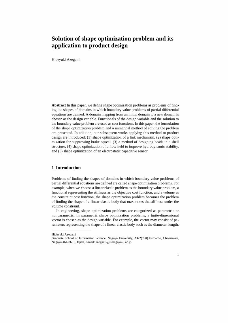
Solution of shape optimization problem and itsapplication to product design
Hideyuki Azegami
Abstract In this paper, we define shape optimization problems as problems of find-ing the shapes of domains in which boundary value problems of partial differentialequations are defined. A domain mapping from an initial domain to a new domain ischosen as the design variable. Functionals of the design variable and the solution tothe boundary value problem are used as cost functions. In this paper, the formulationof the shape optimization problem and a numerical method of solving the problemare presented. In addition, our subsequent works applying this method to productdesign are introduced: (1) shape optimization of a link mechanism, (2) shape opti-mization for suppressing brake squeal, (3) a method of designing beads in a shellstructure, (4) shape optimization of a flow field to improve hydrodynamic stability,and (5) shape optimization of an electrostatic capacitive sensor.
1 Introduction
Problems of finding the shapes of domains in which boundary value problems ofpartial differential equations are defined are called shape optimization problems. Forexample, when we choose a linear elastic problem as the boundary value problem, afunctional representing the stiffness as the objective cost function, and a volume asthe constraint cost function, the shape optimization problem becomes the problemof finding the shape of a linear elastic body that maximizes the stiffness under thevolume constraint.
In engineering, shape optimization problems are categorized as parametric ornonparametric. In parametric shape optimization problems, a finite-dimensionalvector is chosen as the design variable. For example, the vector may consist of pa-rameters representing the shape of a linear elastic body such as the diameter, length,
Hideyuki AzegamiGraduate School of Information Science, Nagoya University, A4-2(780) Furo-cho, Chikusa-ku,Nagoya 464-8601, Japan, e-mail: [email protected]
1
2 Hideyuki Azegami
or thickness. Sometimes the nodal coordinates of a finite-element model, positionsof control points for nonuniform rational B-spline curves or surfaces, or undeter-mined multipliers in a linear combination of basis vectors to determine the bound-ary are used as the parametric design variables. In this formulation, increasing thenumber of design parameters corresponds to increasing the number of dimensionsof the vector space. Consequently, the optimization problem becomes more difficultto solve with increasing number of design parameters.
On the other hand, in nonparametric shape optimization problems, a displace-ment denoting the domain variation from an initial domain to a new domain is se-lected as the design variable. Because the displacement is a function, the nonpara-metric shape optimization problem becomes a functional optimization problem. Inthis problem, the number of design parameters is infinite. Thus, we can expect afiner result than that for parametric optimization problems.
The basic concept of the Gateaux derivative of a cost function with respect todomain variation was presented early in the 20th century [10, 17]. The derivativewas called the shape derivative of the cost function. Subsequently, many researchershave studied the shape derivative (see the citations in [2]). However, the nonpara-metric shape optimization problem is found to be irregular because the regularitiesof the shape derivatives of the cost functions are less than the regularity required tomaintain the original regularity of the initial domain. Methods of compensating forthe lack of regularity of the shape derivative have been presented. Mohammadi andPironneau proposed a method of remaking a smooth boundary by using the Laplaceoperator on the boundary [12]. Another method that introduced the Tikhonov regu-larization term into the cost function was presented by Yamada et al. in the level setapproach [18].
To ensure regularity, the authors have developed another method that uses thegradient method in the Hilbert spaceH1
(Ω ;Rd
)for d ∈ 2,3-dimensional do-
mainsΩ in which boundary value problems of partial differential equations aredefined [1, 6, 5]. In this method, domain variation is obtained as a solution to aboundary value problem of an elliptic partial differential equation, such as a linearelastic problem defined in the current domain using the Neumann condition with thenegative value of the shape derivative on the boundary. Because the Neumann con-dition can be considered as a fictitious traction, we called this method the tractionmethod. This method is similar to methods producing domain variations by fictitiousforces [8, 19, 14]. However, those methods are formulated using parametric designvariables of nodal displacements, whereas the traction method is formulated usingnonparametric design variables of domain variation. Moreover, the traction methodis essentially different from the method using the fictitious linear elastic solution, inwhich the shape derivative is used as the Dirichlet condition [9].
Applications of the traction method to various shape optimization problems inengineering have been reported (see the citations in [2]). Moreover, we previouslypresented a similar method, referred to as theH1 gradient method, for a topologyoptimization problem of density type [4]. Then, in the context of theH1 gradientmethod for the topology optimization problem, we refer to the traction method asthe H1 gradient method for the shape optimization problem [2]. The definition of
Solution of shape optimization problem and its application to product design 3
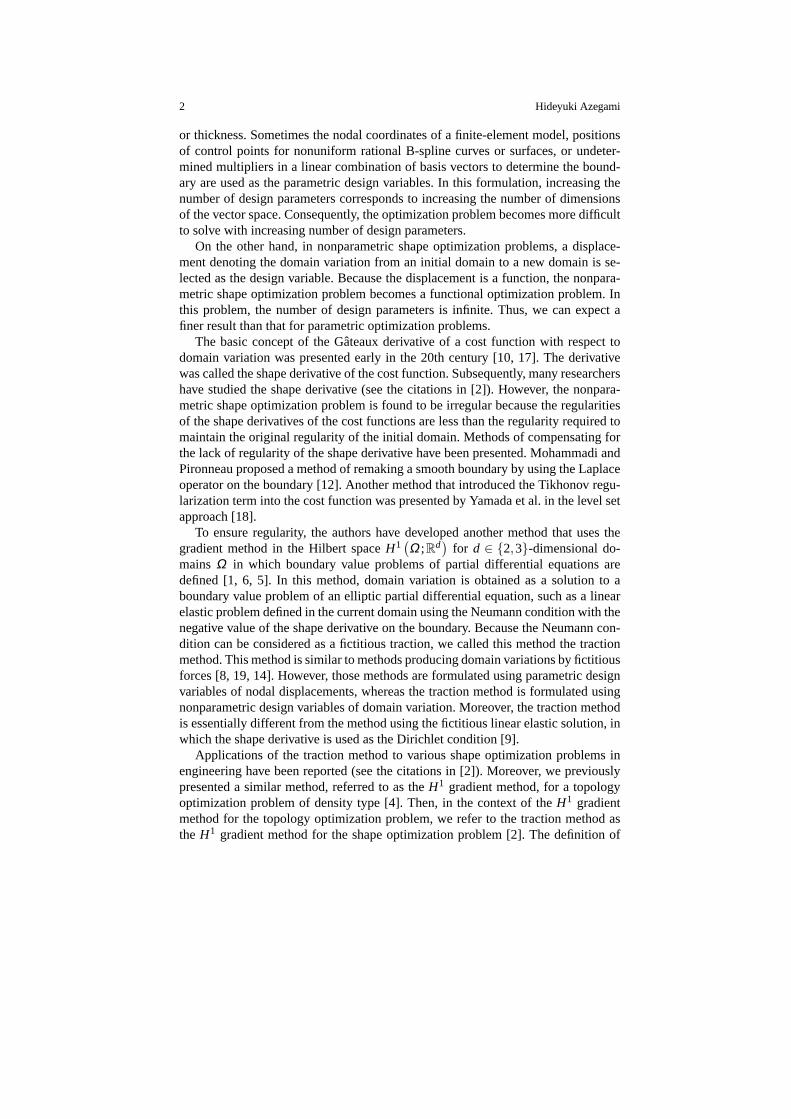
Fig. 1 Initial domainΩ0 ⊂Rd and domain variationφ : Rd → Rd
x
¡D(Á)
¡p(Á)
pN(Á)
b(Á)uD(Á) (Á)
0
(i+Á)(x)
theH1 gradient method and the solution obtained using this method are describedherein.
On the basis of this background, this paper introduces an outline of the formu-lation and solution of a shape optimization problem, and recent results for productdesign obtained using this solution.
In this paper, we use the notationWs,p(Ω0;Rd
)to represent the Sobolev space
for the set of functions defined inΩ0, which has a value ofRd and iss∈ [0,∞] timesdifferentiable andp ∈ [1,∞]-th order Lebesgue integrable. Moreover,Lp
(Ω0;Rd
)andHs
(Ω0;Rd
)are denoted byW0,p andWs,2
(Ω0;Rd
), respectively.
2 Outline of shape optimization problem and its solution
Let us assume that a boundary value problem of partial differential equations isgiven as a linear elastic problem in ad ∈ 2,3-dimensional bounded domainΩ0 ⊂ Rd, the boundary∂Ω0 of which is required to be at least a Lipschitz bound-ary, i.e., locally the graph of a Lipschitz continuous function. We assume thatthe domain varies by deformationφ ∈ D ⊂ X as shown in Fig. 1 and becomesΩ (φ) = (i+φ)(Ω0), wherei denotes the identity mapping. Here, the linear spaceX and the admissible setD of φ are given by
X =
φ ∈ H1(Rd;Rd
) ∣∣∣ φ = 0Rd on ΩC0
, (1)
D =
φ ∈ X∩W1,∞(Rd;Rd
) ∣∣ conditions for bijection, (2)
whereΩC0 is a subset ofΩ0 (¯ denotes closure) previously derived from the designdemands (ΩC0 = /0 in the case of Fig. 1). In the definition ofX, the definition ofφ ∈ X is extended fromΩ0 to Rd on the basis of Calderon’s extension theoremin order to fix the definition of the function in the process of domain variation.H1
(Rd;Rd
)is selected because a Hilbert space is required in order to define a
gradient method later. In the following, we use the notation( ·)(φ) to represent (i +φ)(x) | x ∈ ( ·)0.
4 Hideyuki Azegami
For φ ∈ D , we define a linear elastic problem inΩ (φ). Let u : Ω (φ) → Rd
be an elastic displacement,E(u) =
∇uT +(∇uT
)T/2 be a linear strain,S(u) =
C(φ)E(u) be a stress, andC(φ) : Ω (φ)→Rd×d×d×d denote a stiffness. We denotethe outer unit normal byν .
Problem 2.1 (Linear elastic problem) For φ ∈D and given functionsb(φ), pN (φ),anduD (φ), as shown in Fig. 1, andC(φ), findu such that
−∇TS(φ ,u) = bT (φ) in Ω (φ) , (3)
S(φ ,u)ν = pN (φ) onΓp (φ) , (4)
S(φ ,u)ν = 0Rd onΓN (φ)\ Γp (φ) , (5)
u = uD (φ) onΓD (φ) . (6)
When the given functions are well defined,u−uD is found uniquely in
U =
u ∈ H1(
Ω (φ) ;Rd) ∣∣∣ u = 0Rd onΓD (φ)
. (7)
For later use, we define the Lagrange function of Problem 2.1 as
LM (φ ,u,v) =∫
Ω(φ)(−S(u) ·E(v)+b ·v)dx+
∫Γp(φ)
pN ·v dγ
+∫
ΓD(φ)(u−uD) · (S(v)ν)+v · (S(u)ν)dγ, (8)
wherev ∈U is introduced as the Lagrange multiplier. Ifu is the solution to Problem2.1, the weak form of Problem 2.1 is written as
LM (φ ,u,v) = 0
for all v ∈U .In a shape optimization problem, to find a solutionφ in D , we need a condition
thatu−uD belongs to
S =U ∩W1,∞(
Ω (φ) ;Rd). (9)
Here we assume that the conditions foru−uD ∈ S are satisfied.Using φ and the solutionu to Problem 2.1, we define the cost functions for a
shape optimization problem as
f0 (φ ,u) =∫
Ω(φ)b ·u dx+
∫ΓN(φ)
pN ·u dγ −∫
ΓD(φ)uD · (S(u)ν) dγ, (10)
f1 (φ) =∫
Ω(φ)dx−c1. (11)
Solution of shape optimization problem and its application to product design 5
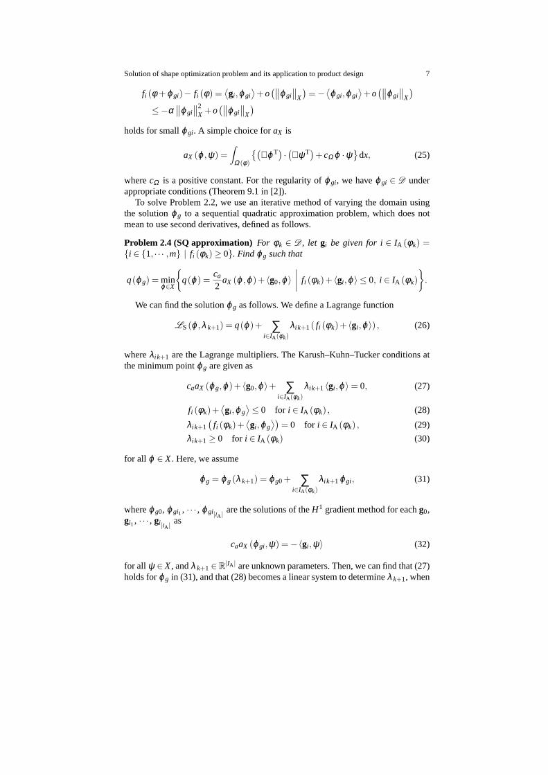
Here, f0 is called the mean compliance representing the deformability of the linearelastic body. Further,f1 is the cost function for the volume constraint, wherec1 isa constant for the volume constraint. The shape optimization problem of the linearelastic body is defined as follows.
Problem 2.2 (Mean compliance minimization problem)For f0 and f1, findΩ (φ)such that
minφ∈D
f0 (φ ,u) | f1 (φ)≤ 0, u−uD ∈ S , Problem 2.1 .
The shape derivatives of the cost functions are evaluated as follows. Becausef0is a functional ofu, which is the solution to Problem 2.1, we define the Lagrangefunction for f0 as
L0 (φ ,u,v0) = f0 (φ ,u)+LM (φ ,u,v0) . (12)
We denoteϕ ∈ X as the domain variation and take the derivative ofL0 with respectto arbitrary variation(ϕ,u′,v′0) ∈ X ×U2 of (φ ,u,v0) ∈ D ×S 2. Then, we havethe following form:
L ′0 (φ ,u,v0)
[ϕ,u′,v′0
]= L0φ ′ (φ ,u,v0) [ϕ ]
+L0u (φ ,u,v0)[u′]+L0v0 (φ ,u,v0)
[v′0]. (13)
For the third term of (13), we have
L0v0 (φ ,u,v0)[v′0]= LMv0 (φ ,u,v0)
[v′0]= LM
(φ ,u,v′0
). (14)
Then, ifu is the solution to Problem 2.1, the third term of (13) becomes 0. Moreover,replacing the second term of (13) with 0, we have a weak form of an adjoint problemto determinev0. In this case, we have
L0u (φ ,u,v0)[u′]= LM
(φ ,v0,u′) . (15)
Then, if we assume the self-adjoint relation
v0 = u, (16)
the second term of (13) becomes 0.Under the above assumptions foru andv0, we have the shape derivative off0
from the first term. Here, we assume thatb, pN, uD, andC are fixed in the initialdomain, which means that they vary with domain variation. Then, applying Propo-sitions A.1 and A.2, which are shown in the Appendix, and using the notationf0 (φ)to representf0 (φ ,u(φ)), we have
6 Hideyuki Azegami
f ′0 (φ) [ϕ ] = L0φ ′ (φ ,u,v0) [ϕ] = ⟨g0,ϕ⟩
=∫
Ω(φ)
(GΩ0 ·∇ϕT +gΩ0∇ ·ϕ
)dx+
∫Γp(φ)
gp0 ·ϕ dγ +∫
∂Γp(φ)∪Θ(φ)g∂ p0 ·ϕ dς ,
(17)
where
GΩ0 = 2S(u)(∇uT)T
, (18)
gΩ0 =−S(u) ·E(u)+2b ·u, (19)
gp0 = 2κ (pN ·u)ν , (20)
g∂ p0 = 2(pN ·u)τ . (21)
Here, the Dirichlet condition in Problem 2.1 was used.Θ (φ) is the set of cornerpoints inΓ (φ) for d = 2 and the vertices and edges ford = 3, τ denotes the tan-gent, andκ = ∇ ·ν . We can confirm thatg0 is included inX′ (the dual space ofX)whenu ∈ S , and we call it the shape gradient off0 as the meaning of the Frechetderivative.
On the other hand, the shape derivativef1 (φ) is obtained using Proposition A.1as
f ′1 (φ) [ϕ ] = ⟨g1,ϕ⟩=∫
Ω(φ)∇ ·ϕ dx. (22)
When we assume thatb, pN, uD, andC are fixed inRd, that is, that they areindependent of the domain variation, we have other results forg0 andg1 given byboundary integrals [3].
Usingg0 andg1, we can apply an iterative algorithm based on a gradient methodin X, which we call theH1 gradient method, to solve Problem 2.2. TheH1 gradientmethod forgi (i ∈ 0,1) is to find the domain variationϕgi ∈ X as the solutionof the following problem. Hereafter, we denotef0 (φ) = f0 (φ ,u(φ)) as f0 (φ) andconsider a problem minimizingf0 (φ) under constraintsf1 (φ)≤ 0, · · · , fm(φ)≤ 0.
Problem 2.3 (H1 gradient method of domain variation type) Let aX : X ×X →R be a bounded coercive bilinear form such that there existαX > 0 andβX > 0 thatsatisfy
aX (ϕ,ϕ)≥ αX ∥ϕ∥2X , |aX (ϕ,ψ)| ≤ βX ∥ϕ∥X ∥ψ∥X (23)
for all ϕ ∈ X andψ ∈ X. For gi ∈ X′, findϕgi ∈ X such that
aX (ϕgi,ψ) =−⟨gi ,ψ⟩ (24)
for all ψ ∈ X.
The solutionϕgi decreasesfi because
Solution of shape optimization problem and its application to product design 7
fi (φ +ϕgi)− fi (φ) =⟨gi ,ϕgi
⟩+o
(∥∥ϕgi∥∥
X
)=−
⟨ϕgi,ϕgi
⟩+o
(∥∥ϕgi∥∥
X
)≤−α
∥∥ϕgi∥∥2
X +o(∥∥ϕgi
∥∥X
)holds for smallϕgi. A simple choice foraX is
aX (ϕ,ψ) =∫
Ω(φ)
(∇ϕT) · (∇ψT)+cΩ ϕ ·ψ
dx, (25)
wherecΩ is a positive constant. For the regularity ofϕgi, we haveϕgi ∈ D underappropriate conditions (Theorem 9.1 in [2]).
To solve Problem 2.2, we use an iterative method of varying the domain usingthe solutionϕg to a sequential quadratic approximation problem, which does notmean to use second derivatives, defined as follows.
Problem 2.4 (SQ approximation) For φ k ∈ D , let gi be given for i∈ IA (φ k) =i ∈ 1, · · · ,m | fi (φ k)≥ 0. Find ϕg such that
q(ϕg) = minϕ∈X
q(ϕ) =
ca
2aX (ϕ ,ϕ)+ ⟨g0,ϕ⟩
∣∣∣∣ fi (φ k)+ ⟨gi ,ϕ⟩ ≤ 0, i ∈ IA (φ k)
.
We can find the solutionϕg as follows. We define a Lagrange function
LS(ϕ,λ k+1) = q(ϕ)+ ∑i∈IA(φk)
λi k+1 ( fi (φ k)+ ⟨gi ,ϕ⟩) , (26)
whereλi k+1 are the Lagrange multipliers. The Karush–Kuhn–Tucker conditions atthe minimum pointϕg are given as
caaX (ϕg,ϕ)+ ⟨g0,ϕ⟩+ ∑i∈IA(φk)
λi k+1 ⟨gi ,ϕ⟩= 0, (27)
fi (φ k)+⟨gi ,ϕg
⟩≤ 0 for i ∈ IA (φ k) , (28)
λi k+1(
fi (φ k)+⟨gi ,ϕg
⟩)= 0 for i ∈ IA (φ k) , (29)
λi k+1 ≥ 0 for i ∈ IA (φ k) (30)
for all ϕ ∈ X. Here, we assume
ϕg = ϕg (λ k+1) = ϕg0+ ∑i∈IA(φk)
λi k+1 ϕgi, (31)
whereϕg0, ϕgi1, · · · , ϕgi|IA |are the solutions of theH1 gradient method for eachg0,
gi1, · · · , gi|IA |as
caaX (ϕgi,ψ) =−⟨gi ,ψ⟩ (32)
for all ψ ∈X, andλ k+1 ∈R|IA | are unknown parameters. Then, we can find that (27)holds forϕg in (31), and that (28) becomes a linear system to determineλ k+1, when
8 Hideyuki Azegami
¡D(Á)
¡p(Á)
pN(Á)
b(Á)uD(Á)
(Á)
¡D(Á)
¡p(Á)=¡´i(Á)
(Á)
gpig
´i
g@pi
g@´i
g i
cG i
(Á+')
(Á)
x '(x)
(a) State determination andadjoint problems (PDE)
(b) H1 gradient method (PDE) (c) Reshaping
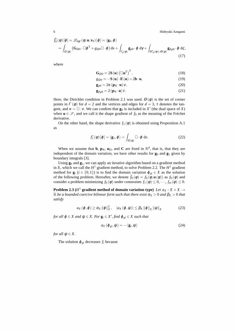
Fig. 2 H1 gradient method for shape optimization. PDE: partial differential equation
“≤” is replaced by “=,” as follows:(⟨gi ,ϕg j
⟩)(i, j)∈I2
A(φk)
(λ j k+1
)j∈IA(φk)
=−(
fi (φ k)+⟨gi ,ϕg0
⟩)i∈IA(φk)
. (33)
In this case, we assume an algorithm to setλi k+1 = 0 for
i ∈ II (φ k) = i ∈ IA (φ k) | λi k+1 < 0 ,
replaceIA (φ k) with IA (φ k) \ II (φ k), and resolve the linear system of (28). WhenII (φ k) becomes /0, the Karush–Kuhn–Tucker conditions are satisfied for smallϕg.Moreover, whenfi (φ k) = 0 for all i ∈ IA (φ k), λ k+1 are determined independentlyof the magnitude ofϕg.
A simple algorithm for solving a shape optimization problem is shown below.
1. SetΩ0 andφ0 = i as f1 (φ0) ≤ 0, · · · , fm(φ0) ≤ 0. Setca, ε0, ε1, · · · , εm appro-priately. Setk= 0.
2. Solve the state determination problem atφ k [Fig. 2 (a)], and computef0 (φ k),f1 (φ k), · · · , fm(φ k). SetIA (φ k) = i ∈ 1, · · · ,m | fi (φ k)≥−εi.
3. Solve adjoint problems atφ k [Fig. 2 (a)], and computeg0, gi1, · · · , gi|IA |.
4. Solveϕg0, ϕgi1, · · · , ϕgi|IA |using (32) [Fig. 2 (b)].
5. Solveλ k+1 using (33). WhenII (φ k) = /0, replaceIA (φ k) \ II (φ k) with IA (φ k),and resolve (33) untilII (φ k) = /0.
6. Computeϕg using (31), setφ k+1 = φ k+ϕg [Fig. 2 (c)], and computef0 (φ k+1),f1 (φ k+1), · · · , fm(φ k+1). SetIA (φ k+1) = i ∈ 1, · · · ,m | fi (φ k+1)≥−εi.
7. Assess| f0 (φ k+1)− f0 (φ k)| ≤ ε0.
• If “Yes,” proceed to (8).• If “No,” replacek+1 with k and return to (3).
8. Stop the algorithm.
Figure 3 shows a numerical result for Problem 2.2 computed by a program de-veloped using FreeFEM++[11].
Solution of shape optimization problem and its application to product design 9
¡D0
¡p0
¡D0
pN
(a) Initial shape and boundary condition (b) Optimized shape
Fig. 3 Numerical result for mean compliance minimization problem
xL1
xL2
xL3
01
02
03 ¡p p3
b1
1
xG1
xG1
µ1
x
u1(q1,x)
01
(a) Boundary conditions (b) Rigid motion ofΩ01
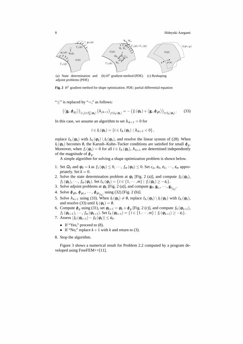
Fig. 4 Link mechanism
(a) Initial shapes (b) Optimum shapes
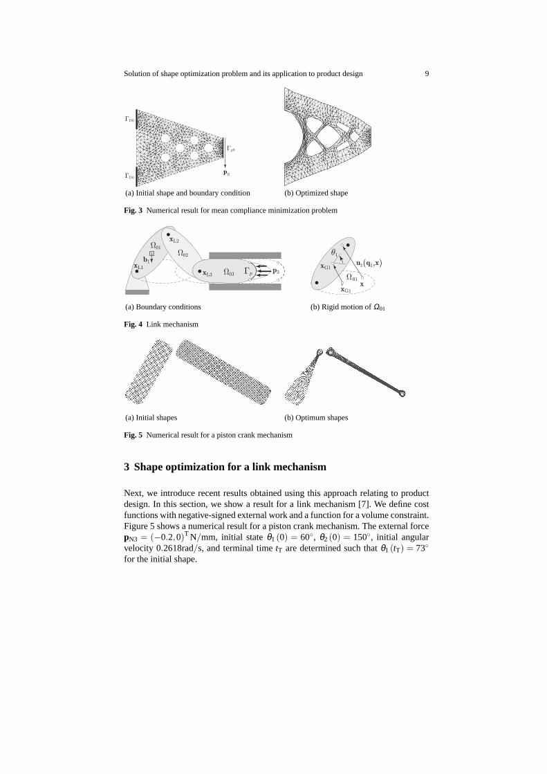
Fig. 5 Numerical result for a piston crank mechanism
3 Shape optimization for a link mechanism
Next, we introduce recent results obtained using this approach relating to productdesign. In this section, we show a result for a link mechanism [7]. We define costfunctions with negative-signed external work and a function for a volume constraint.Figure 5 shows a numerical result for a piston crank mechanism. The external forcepN3 = (−0.2,0)T N/mm, initial stateθ1 (0) = 60, θ2 (0) = 150, initial angularvelocity 0.2618rad/s, and terminal timetT are determined such thatθ1 (tT) = 73
for the initial shape.
10 Hideyuki Azegami
R0P0
¡P0, ¡R0
Coulomb friction
¡D0 ¡P0
¡R0
®, ¹
ºP
¿PºP
¿R R0
P0
(a) Pad and rotor (b) Coulomb friction betweenΓR0 andΓP0
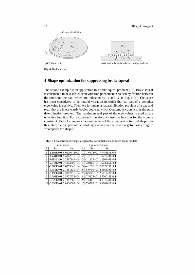
Fig. 6 Brake model
4 Shape optimization for suppressing brake squeal
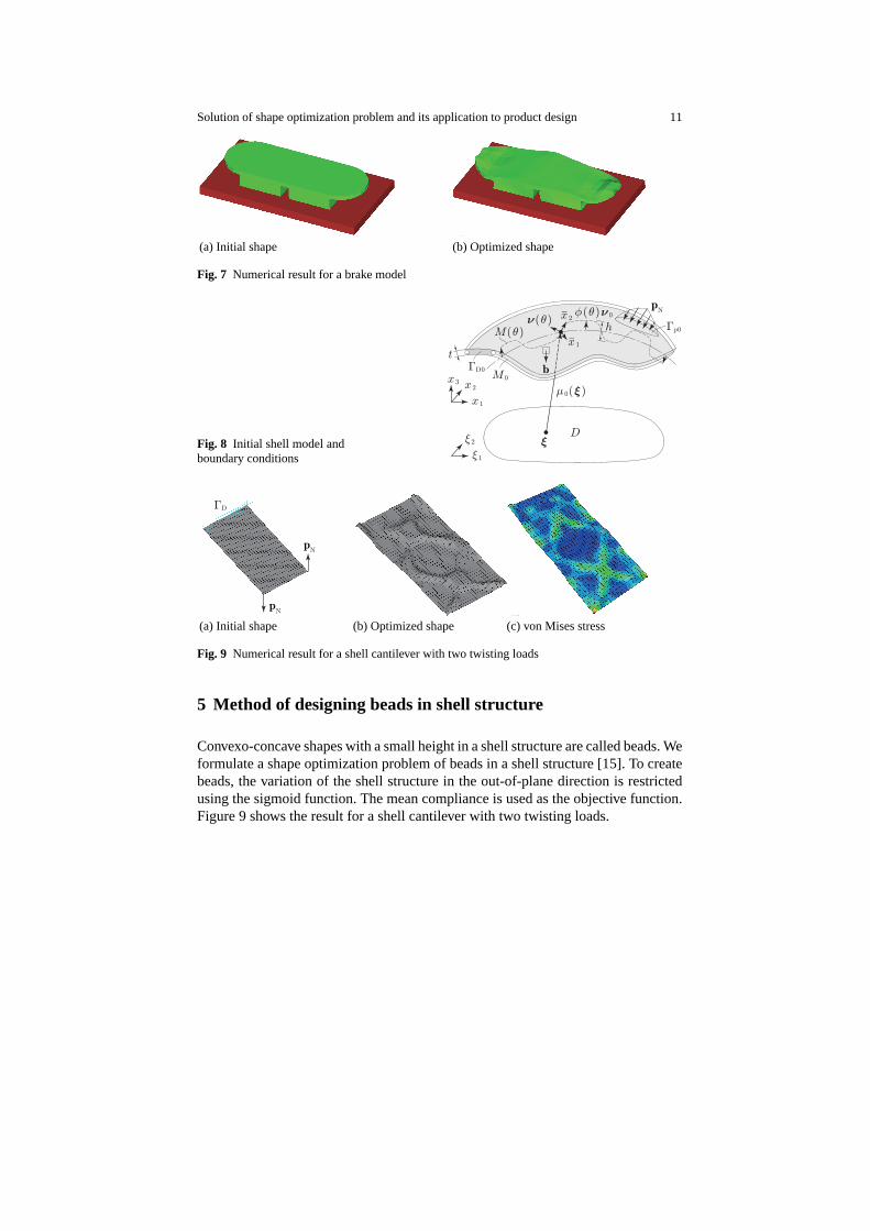
The second example is an application to a brake squeal problem [16]. Brake squealis considered to be a self-excited vibration phenomenon caused by friction betweenthe rotor and the pad, which are indicated byτP andτR in Fig. 6 (b). The causehas been considered to be natural vibration in which the real part of a complexeigenvalue is positive. Then, we formulate a natural vibration problem of a pad androtor that are linear elastic bodies between which Coulomb friction acts as the statedetermination problem. The maximum real part of the eigenvalues is used as theobjective function. For a constraint function, we use the function for the volumeconstraint. Table 1 compares the eigenvalues of the initial and optimized shapes. Inthis table, the real part of the third eigenvalue is reduced to a negative value. Figure7 compares the shapes.
Table 1 Comparison of complex eigenvalues of initial and optimized brake models
Initial shape Optimized shapek Re Im
1 -1.692E+018.022947E+032 -1.444E+019.438261E+033 8.613E+001.249724E+044 -2.944E+011.437360E+045 -5.783E+011.629984E+046 -5.356E+012.168113E+047 -5.195E+012.394771E+048 -6.593E+012.573753E+049 -6.325E+012.711726E+0410 -6.896E+012.893466E+04
k Re Im
1 -1.647E+017.745197E+032 -1.765E+011.027973E+043 -1.163E+011.110440E+044 -3.048E+011.503565E+045 -4.185E+012.092213E+046 -5.070E+012.186379E+047 -6.588E+012.671747E+048 -7.522E+012.756015E+049 -7.540E+013.137934E+0410 -7.658E+013.320161E+04
Solution of shape optimization problem and its application to product design 11
(a) Initial shape (b) Optimized shape
Fig. 7 Numerical result for a brake model
Fig. 8 Initial shell model andboundary conditions
M 0
Á(µ)º 0º(µ)
M(µ)x 1
x 2
t
h
¡D0
¡p0
pN
b
D
» 1
» 2
¹ 0(»)
»
x 1
x 2x 3
¹
¹
¡D
pN
pN
(a) Initial shape (b) Optimized shape (c) von Mises stress
Fig. 9 Numerical result for a shell cantilever with two twisting loads
5 Method of designing beads in shell structure
Convexo-concave shapes with a small height in a shell structure are called beads. Weformulate a shape optimization problem of beads in a shell structure [15]. To createbeads, the variation of the shell structure in the out-of-plane direction is restrictedusing the sigmoid function. The mean compliance is used as the objective function.Figure 9 shows the result for a shell cantilever with two twisting loads.
12 Hideyuki Azegami
(a) Initial shape
(b) Optimized shape
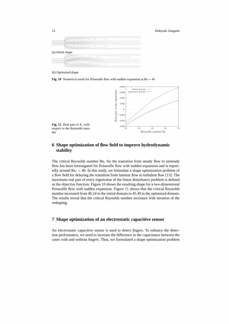
Fig. 10 Numerical result for Poiseuille flow with sudden expansion atRe= 45
Fig. 11 Real part ofλ1 withrespect to the Reynolds num-ber
¡0.006
¡0.004
¡0.002
0
0.002
0.004
0.006
0.008
35 40 45 50 55
Rea
l par
t of
the
eige
nval
ue
Reynolds number Re
Initial domainOptimized domain
6 Shape optimization of flow field to improve hydrodynamicstability
The critical Reynolds number Rec for the transition from steady flow to unsteadyflow has been investigated for Poiseuille flow with sudden expansion and is report-edly around Rec = 40. In this study, we formulate a shape optimization problem ofa flow field for delaying the transition from laminar flow to turbulent flow [13]. Themaximum real part of every eigenvalue of the linear disturbance problem is definedas the objective function. Figure 10 shows the resulting shape for a two-dimensionalPoiseuille flow with sudden expansion. Figure 11 shows that the critical Reynoldsnumber increased from 40.24 in the initial domain to 45.49 in the optimized domain.The results reveal that the critical Reynolds number increases with iteration of thereshaping.
7 Shape optimization of an electrostatic capacitive sensor
An electrostatic capacitive sensor is used to detect fingers. To enhance the detec-tion performance, we need to increase the difference in the capacitance between thecases with and without fingers. Thus, we formulated a shape optimization problem
Solution of shape optimization problem and its application to product design 13
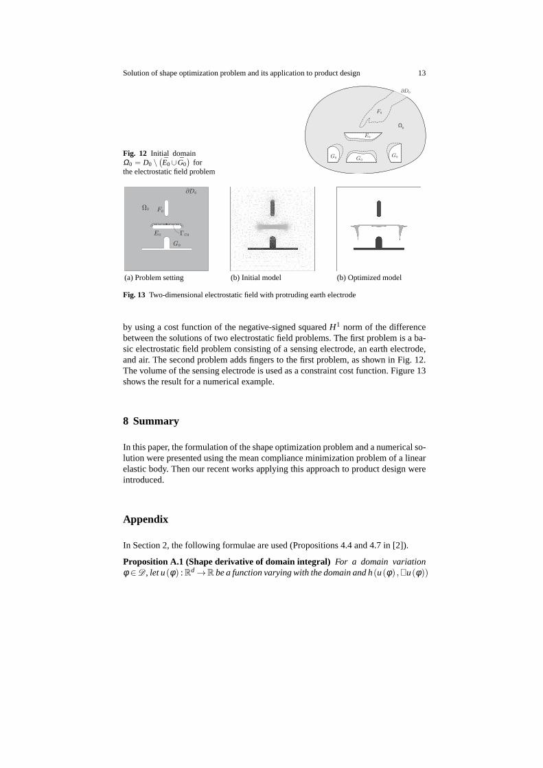
Fig. 12 Initial domainΩ0 = D0 \
(E0∪ G0
)for
the electrostatic field problem
E0
F0
G0 G0G0
@D0
Ω0
E0
F0
G0
0
@D0
¡C0
(a) Problem setting (b) Initial model (b) Optimized model
Fig. 13 Two-dimensional electrostatic field with protruding earth electrode
by using a cost function of the negative-signed squaredH1 norm of the differencebetween the solutions of two electrostatic field problems. The first problem is a ba-sic electrostatic field problem consisting of a sensing electrode, an earth electrode,and air. The second problem adds fingers to the first problem, as shown in Fig. 12.The volume of the sensing electrode is used as a constraint cost function. Figure 13shows the result for a numerical example.
8 Summary
In this paper, the formulation of the shape optimization problem and a numerical so-lution were presented using the mean compliance minimization problem of a linearelastic body. Then our recent works applying this approach to product design wereintroduced.
Appendix
In Section 2, the following formulae are used (Propositions 4.4 and 4.7 in [2]).
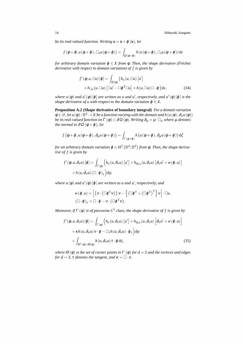
Proposition A.1 (Shape derivative of domain integral)For a domain variationφ ∈D , let u(φ) :Rd →R be a function varying with the domain and h(u(φ) ,∇u(φ))
14 Hideyuki Azegami
be its real-valued function. Writingz= x+ϕ (x), let
f (φ +ϕ ,u(φ +ϕ) ,∇zu(φ +ϕ)) =∫
Ω(φ+ϕ)h(u(φ +ϕ) ,∇zu(φ +ϕ))dz
for arbitrary domain variationϕ ∈ X from φ . Then, the shape derivative (Frechetderivative with respect to domain variation) of f is given by
f ′ (φ ,u,∇u) [ϕ] =∫
Ω(φ)
hu (u,∇u)
[u′]
+h∇u (u,∇u)[∇u′−∇ϕT∇u
]+h(u,∇u)∇ ·ϕ
dx, (34)
where u(φ) and u′ (φ) [ϕ] are written as u and u′, respectively, and u′ (φ) [ϕ ] is theshape derivative of u with respect to the domain variationϕ ∈ X.
Proposition A.2 (Shape derivative of boundary integral) For a domain variationφ ∈D , let u(φ) :Rd →R be a function varying with the domain and h(u(φ) ,∂νu(φ))be its real-valued function onΓ (φ)⊂ ∂Ω (φ). Writing∂µ = µ ·∇z, whereµ denotesthe normal to∂Ω (φ +ϕ), let
f(φ +ϕ ,u(φ +ϕ) ,∂µu(φ +ϕ)
)=
∫Γ (φ+ϕ)
h(u(φ +ϕ) ,∂µu(φ +ϕ)
)dζ
for an arbitrary domain variationϕ ∈ H2(Rd;Rd
)fromφ . Then, the shape deriva-
tive of f is given by
f ′ (φ ,u,∂νu) [ϕ ] =∫
Γ (φ)
(hu (u,∂νu)
[u′]+h∂ν u (u,∂νu)
[∂νu′+w(ϕ,u)
]+h(u,∂νu)(∇ ·ϕ)τ
)dγ,
where u(φ) and u′ (φ) [ϕ ] are written as u and u′, respectively, and
w(ϕ,u) =[
ν ·(∇ϕTν
)ν −
(∇ϕT +
(∇ϕT)T
ν]·∇u,
(∇ ·ϕ)τ = ∇ ·ϕ −ν ·(∇ϕTν
).
Moreover, ifΓ (φ) is of piecewise C2 class, the shape derivative of f is given by
f ′ (φ ,u,∂νu) [ϕ ] =∫
Γ (φ)
(hu (u,∂νu)
[u′]+h∂ν u (u,∂νu)
[∂νu′+w(ϕ,u)
]+κh(u,∂νu)ν ·ϕ −∇τh(u,∂νu) ·ϕτ
)dγ
+∫
∂Γ (φ)∪Θ(φ)h(u,∂νu)τ ·ϕ dς , (35)
whereΘ (φ) is the set of corner points inΓ (φ) for d = 2 and the vertices and edgesfor d = 3, τ denotes the tangent, andκ = ∇ ·ν .
Solution of shape optimization problem and its application to product design 15
References
1. Azegami, H.: A solution to domain optimization problems (in Japanese). Trans. of Jpn. Soc.of Mech. Engs., Ser. A60(574), 1479–1486 (1994)
2. Azegami, H.: Regularized solution to shape optimization problem (in Japanese). Transactionsof the Japan Society for Industrial and Applied Mathematics23(2), 83–138 (2014)
3. Azegami, H., Fukumoto, S., Aoyama, T.: Shape optimization of continua using NURBS asbasis functions. Structural and Multidisciplinary Optimization47(2), 247–258 (2013)
4. Azegami, H., Kaizu, S., Takeuchi, K.: Regular solution to topology optimization problems ofcontinua. JSIAM Letters3, 1–4 (2011)
5. Azegami, H., Takeuchi, K.: A smoothing method for shape optimization: Traction method us-ing the Robin condition. International Journal of Computational Methods3(1), 21–33 (2006)
6. Azegami, H., Wu, Z.Q.: Domain optimization analysis in linear elastic problems: Approachusing traction method. JSME International Journal Series A39(2), 272–278 (1996)
7. Azegami, H., Zhou, L., Umemura, K., Kondo, N.: Shape optimization for a link mechanism.Structural and Multidisciplinary Optimization48(1), 115–125 (2013)
8. Belegundu, A.D., Rajan, S.D.: A shape optimization approach based on natural designvaraibles and shape functions. Comput. Methods Appl. Mech. Engrg.66, 87–106 (1988)
9. Choi, K.K., Kim, N.H.: Structural sensitivity analysis and optimization, 1 & 2. Springer, NewYork (2005)
10. Hadamard, J.: Memoire des savants etragers. Oeuvres de J. Hadamard, chap. Memoire sur leprobleme d’analyse relatifa l’equilibre des plaqueselastiques encastrees, Memoire des savantsetragers, Oeuvres de J. Hadamard, pp. 515–629. CNRS, Paris (1968)
11. Hecht, F.: New development in freefem++. J. Numer. Math.20(3-4), 251–265 (2012)12. Mohammadi, B., Pironneau, O.: Applied shape optimization for fluids. Oxford University
Press, Oxford, New York (2001)13. Nakazawa, T., Azegami, H.: Shape optimization of flow field improving hydrodynamic sta-
bility. Japan Journal of Industrial and Applied Mathematics Japan Journal of Industrial andApplied Mathematics (2015). Accepted
14. Scherer, M., Denzer, R., Steinmann, P.: A fictitious energy approach for shape optimization.Int. J. Numer. Meth. Engng.82, 269–302 (2010)
15. Shintani, K., Azegami, H.: A design method of beads in shell structure using non-parametricshape optimization method. In: Proceedings of the the ASME 2014 International DesignEngineering Technical Conferences & Computers and Information in Engineering Conference(IDETCCIE 2014) (eBook), pp. 1–8 (2014)
16. Shintani, K., Azegami, H.: Shape optimization for suppressing brake squeal. Structural andMultidisciplinary Optimization50(6), 1127–1135 (2014)
17. Sokolowski, J., Zolesio, J.P.: Introduction to Shape Optimization: Shape Sensitivity Analysis.Springer-Verlag, New York (1992)
18. Yamada, T., Izui, K., Nishiwaki, S., Takezawa, A.: A topology optimization method based onthe level set method incorporating a fictitious interface energy. Comput. Methods Appl. Mech.Engrg.199, 2876–2891 (2010)
19. Yao, T.M., Choi, K.K.: 3-d shape optimal design and automatic finite element regridding. Int.J. Numer. Meth. Engng.28, 369–384 (1989)