Geodesic Convolutional Shape Optimization

Geodesic Convolutional Shape Optimization

Pierre Baque * 1 Edoardo Remelli * 1 Francois Fleuret 2 1 Pascal Fua 1

AbstractAerodynamic shape optimization has many indus-trial applications. Existing methods, however, areso computationally demanding that typical engi-neering practices are to either simply try a limitednumber of hand-designed shapes or restrict one-self to shapes that can be parameterized usingonly few degrees of freedom.

In this work, we introduce a new way to opti-mize complex shapes fast and accurately. To thisend, we train Geodesic Convolutional Neural Net-works to emulate a fluidynamics simulator. Thekey to making this approach practical is remesh-ing the original shape using a poly-cube map,which makes it possible to perform the computa-tions on GPUs instead of CPUs. The neural netis then used to formulate an objective functionthat is differentiable with respect to the shape pa-rameters, which can then be optimized using agradient-based technique. This outperforms state-of-the-art methods by 5 to 20% for standard prob-lems and, even more importantly, our approachapplies to cases that previous methods cannot han-dle.

1. IntroductionOptimizing the aerodynamic or hydrodynamic propertiesis key to designing shapes, such as those of aircraft wings,windmill blades, hydrofoils, car bodies, bicycle shells, orsubmarine hulls. However, it remains challenging and com-putationally demanding because existing ComputationalFluid Dynamics (CFD) techniques rely either on solving theNavier-Stokes equations or on Lattice Boltzmann methods.Since the simulation must be re-run each time an engineerwishes to change the shape, this makes the design processslow and costly. A typical engineering approach is thereforeto test only a few designs without a fine-grained search inthe space of potential variations.

*Equal contribution 1CVLab, EPFL, Lausanne, Switzerland2Machine Learning Group, Idiap, Martigny, Switzerland. Corre-spondence to: Pierre Baque <[email protected]>.

−∇XG −∇XG

GCNN

GCNNXtrain

Xtest

F yω (Xtrain)

F yω (Xtest)

F zω(Xtrain)

F zω(Xtest)

G(X)

G(X) G(X)

(c)

(b)

(a)

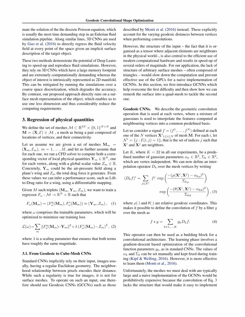
Figure 1. Car shape optimization. (a) We train a GCNN to emulatea CFD simulator and predict from the shape on the left pressuresshown as colors in the middle and drag shown as a gray vertical baron the right. (b) Convolutional layers enable the GCNN to makeaccurate predictions on previously unseen shapes, such as thoseof cars. (c) We use the GCNN to express drag as a differentiablefunction of the mesh vertex positions. Finally, we minimize itunder constraints to produce the rightmost shape.

This is a severe limitation and there have been many at-tempts at overcoming it, but none has been entirely suc-cessful yet. Most current algorithms rely on combiningevolutionary algorithms with heuristic local search (Orman& Durmus, 2016) and complex adjoint methods (Allaire,2015; Gao et al., 2017), which requires rerunning a simula-tion at each iteration step and therefore remains costly. Aclassical approach to reduce the computational complexityis to use Gaussian Process (GP) regressors trained to inter-polate the performance landscape given a low dimensionalparametrization of the shape space. This interpolator isthen used as a proxy for the true objective to speed-up thecomputation, which is referred to as Kriging in the CFD liter-ature (Toal & Keane, 2011; Xu et al., 2017). However, thoseregressors are only effective for shape deformations that canbe parameterized using relatively few parameters (Bengioet al., 2006) and their performance therefore hinges on awell-designed parameterization. Furthermore, the regressorsare specific to a particular parameterization and pre-existingcomputed simulation data using different ones cannot beeasily leveraged.

By contrast, we propose an approach to optimizing the aero-

arX

iv:1

802.

0401

6v1

[cs

.CE

] 1

2 Fe

b 20

18


dynamic or hydrodynamic properties of arbitrarily complexshapes by training Geodesic Convolutional Neural Networks(GCNNs) (Monti et al., 2016) to emulate a fluidynamicssimulator. More specifically, given a set of generic surfacesparametrized as meshes, we train a GCCN to predict theiraerodynamic characteristics, as computed by standard CFDpackages, such as XFoil (Drela, 1989) or Ansys Fluent (Inc.,2011), which are then used to write an objective function.Since this function is differentiable with respect to the vertexcoordinates, we can use it in conjunction with a gradient-based optimization to explore the shape space much fasterand thoroughly than was possible before, with a much betteraccuracy and without putting undue restrictions on the rangeof potential shapes. Since performing convolutions on anarbitrary mesh is much slower than on a regular grid, the keyto making this approach practical is remeshing the originalshape using a cube or poly-cube map (Tarini et al., 2004).It makes it possible to perform the GCNN computations onGPUs instead of CPUs, as for normal CNNs.

In short, our contribution is a new surrogate model methodfor shape optimization. It does not rely on handcraftedfeatures and can handle shapes that must be parameterizedusing many parameters. Since it operates directly on the 3Dsurfaces, an added benefit is that it can leverage training dataproduced using any kind of parameterization and not onlythe specific one used to perform the shape optimization.Fig 1 illustrates the process. The training shapes can bevery different from the target one, which gives our systemflexibility.

We demonstrate that our method outperforms GP ap-proaches, widely used in the industry, both in terms ofregression accuracy and optimization capacity. Not onlydo we improve upon GP optimization by 5% to 20% fora lift maximization task on 2D NACA airfoils involvingfew parameters, but we can also deliver results on fully 3Dshapes for which our baselines perform poorly.

2. Related WorkThere is a massive body of literature about fluid simulationtechniques. Traditional ones rely on numerical discretiza-tion of the Navier-Stokes Equations (NSE) using finite-difference, finite-element, or finite volume methods (Quar-teroni & Quarteroni, 2009; Skinner & Zare-Behtash, 2018).Since the NSE are highly non-linear, the space has to be veryfinely discretized for good accuracy, which tends to makesuch methods computationally expensive. In some cases, ap-proaches such as the Lattice-Boltzmann Method (LBM) (Mc-Namara & Zanetti, 1988), which simulates streaming andcollision processes across individual fluid particles to re-cover the global behavior as an emergent property, can bemore accurate, at the cost of being even more computation-ally expensive (Xian & Takayuki, 2011).

All the above-mentioned techniques approximate the fluo-dynamics for a fixed physical shape and without changingit. A common engineering practice is therefore to first usethem to compute the characteristics of a few hand-designedshapes and then to pick the one giving the best results. Inthis paper, our focus is on using a Deep Learning approachto automate this process by casting it as a gradient descentminimization. In the remainder of this section, we there-fore review existing approaches to shape optimization in theCFD context and then discuss current uses of Deep Learningin that field.

2.1. Shape Optimization

A popular and relatively easy to implement approach toshape optimization relies on genetic algorithms (Gosselinet al., 2009) to explore the space of possible shapes. How-ever, since genetic algorithms require many evaluation of thefitness function, a naive implementation would be inefficientbecause each one requires an expensive CFD simulation.

This can be avoided using Adjoint Differentiation (Allaire,2015; Gao et al., 2017) instead. It involves approximat-ing the solution of a so-called adjoint form of the NSE tocompute the gradient of the fitness function with respect tothe 3D simulation mesh parameters. This allows the useof gradient-based optimization techniques but is still veryexpensive because it requires a new simulation to be run ateach iteration (Alexandersen et al., 2016).

As a result, there has been extensive research in ways toreduce the required number of evaluations of the fitnessfunction. One of the most widely used one relies either onGaussian Processes (GPs, Rasmussen & Williams, 2006),which is known as kriging in the CFD community (Jeonget al., 2005; Toal & Keane, 2011; Xu et al., 2017), or onArtificial Neural Networks (ANN, Gholizadeh & Seyed-poor, 2011; Lundberg et al., 2015; Preen & Bull, 2015) tocompute surrogates or meta-models that approximate thefitness function while being much easier to compute. Bothapproaches can be used either to simply speed-up geneticalgorithms (Ulaganathan & Asproulis, 2013) or to find anoptimal trade-off between exploration and exploitation, us-ing the confidence bounds provided by the GPs to optimizea multi-objective Pareto front. However, these methods alldepend on handcrafted shape parameterizations that can bedifficult to design. Furthermore this makes it necessary toretrain the regressor for each new scenario in which theparameterization changes.

2.2. Deep Learning

As in many other engineering fields, Deep Learning wasrecently introduced in CFD. For example, Neural Networksare used by Tompson et al. (2016) to accelerate Eulerianfluid simulations. This is done by training CNNs to approxi-


mate the solution of the the discrete Poisson equation, whichis usually the most time demanding step in an Eulerian fluidsimulation pipeline. Along similar lines, 3D CNNs are usedby Guo et al. (2016) to directly regress the fluid velocityfield at every point of the space given an implicit surfacedescription of the target object.

These two methods demonstrate the potential of Deep Learn-ing to speed-up and reproduce fluid simulations. However,they rely on 3D CNNs which have a large memory footprintand are extremely computationally demanding whereas theobject of interest is intrinsically represented as 2D manifold.This can be mitigated by running the simulations over acoarse space discretization, which degrades the accuracy.By contrast, our proposed approach directly runs on a sur-face mesh representation of the object, which enables us touse one less dimension and thus considerably reduce thecomputing requirements.

3. Regression of physical quantitiesWe define the set of meshesM⊂ R3N × {0, 1}N×N andM = (X, E) ∈ M , a mesh as being a pair composed oflocations of vertices, and their connectivity.

Let us assume we are given a set of meshes Mm =(Xm, Em), m = 1, . . . ,M, and let us further assume thatfor each one, we ran a CFD solver to compute both a corre-sponding vector of local physical quantities Ym ∈ RN , onefor each vertex, along with a global scalar value Zm ∈ R.Concretely, Ym could be the air-pressure field along aplane’s wing and Zm the total drag force it generates. Fromthese values we can infer a performance score, such as Lift-to-Drag ratio for a wing, using a differentiable mapping.

Given M such triplets (Mm,Ym, Zm), we want to train aregressor Fω :M→ RN × R such that

Fω(Mm) = (F yω(Mm), F zω(Mm)) ≈ (Ym, Zm) , (1)

where ω comprises the trainable parameters, which will beoptimized to minimize our training loss

L(ω)=∑m

‖F yω(Mm)−Ym‖2+λ (F zω(Mm)−Zm)2, (2)

where λ is a scaling parameter that ensures that both termshave roughly the same magnitude.

3.1. From Geodesic to Cube-Mesh CNNs

Standard CNNs implicitly rely on their input, images usu-ally, having a regular Euclidean geometry. The neighbor-hood relationship between pixels encodes their distance.While such a regularity is true for images, it is not forsurface meshes. To operate on such an input, one there-fore should use Geodesic CNNs (GCCNs) such as those

described by Monti et al. (2016) instead. These explicitlyaccount for the varying geodesic distances between verticeswhen performing convolutions.

However, the structure of the input – the fact that it is or-ganised as a tensor where adjacent elements are neighboursin the physical world–, is also central to the efficient use ofmodern computational hardware and results in speed-up ofseveral orders of magnitude. For our application, the lack ofstructure of arbitrary surface meshes – often composed oftriangles – would slow down the computation and preventeffective use of the GPUs for a naive implementation ofGCNNs. In this section, we first introduce GCNNs whichhelp overcome the first difficulty and then show how we canremesh the surface into a quad-mesh to tackle the secondone.

Geodesic CNNs. We describe the geometric convolutionoperation that is used at each vertex, where a mixture ofgaussians is used to interpolate the features computed atneighbouring vertices into a common predefined basis.

Let us consider a signal f = (f1, . . . , fN ) defined at eachone of the N vertices Xi

1≤i≤N of mesh M. For each i, letN i = {j : E(i, j) = 1}, that is the set of indices j such thatXi and Xj are neighbors.

Let K, where K = 32 in all our experiments, be a prede-fined number of gaussian parameters αk ∈ R2, Σk ∈ R2,which are vertex independent. We can now define an inter-polation operator Dk over the mesh vertices by writing

(Dkf)i =∑j∈N i

f j exp

(−(ρ(Xi,Xj)− αkρ)2Σkρ

)

exp

(−(θ(Xi,Xj)− αkθ)2Σkθ

), (3)

where ρ(·) and θ(·) are relative geodesic coordinates. Thismakes it possible to define the convolution of f by a filter gover the mesh as

f ? g =∑

k∈1,...,K

gkDkf. (4)

This operator can then be used as a building block for aconvolutional architecture. The learning phase involves agradient-descent based optimization of the convolutionalfunction parameters gk, as in standard CNNs. The values ofαk and Σk can be set manually and kept fixed during train-ing (Kipf & Welling, 2016). However, it is more effectiveto learn them (Monti et al., 2016).

Unfortunately, the meshes we must deal with are typicallylarge and a naive implementation of the GCNNs would beprohibitively expensive because the convolution of Eq. 3lacks the structure that would make it easy to implement


(a) (b)

(c)(d)

quadre-meshing

gridextraction

volumetricdeformation

projection

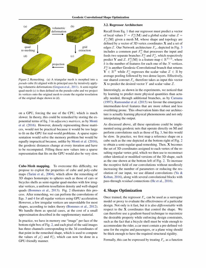
Figure 2. Remeshing. (a) A triangular mesh is morphed into apseudo cube (b) aligned with its principal axes by iteratively apply-ing volumetric deformations (Gregson et al., 2011). A semi-regularquad-mesh (c) is then defined on the pseudo-cube and we projectits vertices onto the original mesh to create the regular tesselationof the original shape shown in (d).

on a GPU, forcing the use of the CPU, which is muchslower. In theory, this could be remedied by storing the ex-ponential terms of Eq. 3 in adjacency matrices, as by Montiet al. (2016). However, densely representing those matri-ces, would not be practical because it would be too largeto fit on the GPU for real-world problems. A sparse repre-sentation would solve the memory problem but would beequally impractical because, unlike by Monti et al. (2016),the geodesic distances change at every iteration and haveto be recomputed. Filling these new values into a sparserepresentation that fits on the GPU would also be very slow.

Cube-Mesh mapping. To overcome this difficulty, wepropose to exploit the properties of cube and poly-cubemaps (Tarini et al., 2004), which allow the remeshing of3D shapes homotopic to spheres such as those of cars orbicycles shells as semi-regular quad-meshes with few irreg-ular vertices, a uniform tessellation density and well-shapedquads (Bommes et al., 2013). Fig. 2 illustrates this pro-cess. After remeshing, we can perform the convolutions ofEqs. 3 and 4 for all regular vertices using GPU acceleration.However, a few irregular vertices are unavoidable for mostshapes, according to index theory (Bommes et al., 2012).We handle them as special cases, at the cost of a smallapproximation described in the supplementary material.

In practice, we have in memory one “image” per face of thebottom-right box of Fig. 2, and each pixel of the said imageshas three channels corresponding to the 3d coordinates ofthat point in the remeshed shape, which is used to computethe values of ρ() and θ(), which can now be done in aGPU-friendly manner.

3.2. Regressor Architecture

Recall from Eq. 1 that our regressor must predict a vectorof local values Y = F yω(M) and a global scalar value Z =F zω(M) given a mesh M, whose shape and topology aredefined by a vector of 3D vertex coordinates X and a set ofedges E . Our Network architecture Fω, depicted in Fig. 3includes a common part F 0

ω that processes the input andfeeds two separate branches F yω and F zω , which respectivelypredict Y and Z. F 0

ω(M) is a feature map ∈ RN×k, wherek is the number of features for each one of the N vertices.F yω is another Geodesic-Convolutional branch that returnsY ∈ RN while F zω regresses the scalar value Z ∈ R byaverage pooling followed by two dense layers. Effectively,our shared convnet Fω therefore takes as input this vectorX to predict the desired vector Y and scalar value Z.

Interestingly, as shown in the experiments, we noticed thatby learning to predict more physical quantities than actu-ally needed, through additional branches, as by Caruana(1997); Ramsundar et al. (2015) we favour the emergenceintermediate-level features that are more robust and lessoverfitting prone. This observation hints that our architec-ture is actually learning physical phenomenons and not onlyinterpolating the output.

As discussed above, all these operations could be imple-mented using geodesic nets that operate directly on M andperform convolutions such as those of Eq. 3, but this wouldbe slow. In practice, we first map a reference shape on acube such as the one depicted at the bottom right of Fig. 2to obtain a semi-regular quad-remeshing. Then, X becomesthe set of 3D coordinates assigned to each vertex of the re-sulting regular vertex grid, which we then use to reconstructeither identical or modified versions of the 3D shape, suchas the one shown at the bottom left of Fig. 2. To increasethe receptive field of our convolutions without needlesslyincreasing the number of parameters or reducing the res-olution of our input, we use dilated convolutions (Yu &Koltun, 2016), along with several convolutional blocks withpass-through residual connections (He et al., 2016).

4. Shape OptimizationOnce trained, the regressor Fω can be used as a surrogatemodel or proxy to evaluate the effectiveness of a particulardesign. Not only is it fast, but it is also differentiable withrespect to the X coordinates that control the shape. Wecan therefore use a gradient-based technique to maximizethe desirable property while enforcing design constraints,such as the fact that a bicycle shell must be wide enough toaccommodate the rider, a car must contain a pre-defined vol-ume for the engine and passengers, or a plane wing shouldbe thick enough to have the required structural rigidity.

Formally, this can be expressed by treating Fω as a function


{X

F yω

F zω

F 0ω

Atrous geoconv

Atrous geoconv block

Residualconnection

Meanpooling

Fully connectedlayer

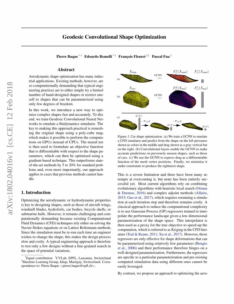
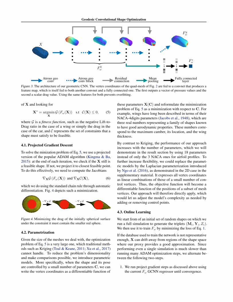
Figure 3. The architecture of our geometric CNN. The vertex coordinates of the quad-mesh of Fig. 2 are fed to a convnet that produces afeature map, which is itself fed to both another convnet and a fully connected one. The first outputs a vector of pressure values and thesecond a scalar drag value. Using the same features for both prevents overfitting.

of X and looking for

X∗ = argminX

G (Fω(X)) s.t C(X) ≤ 0, (5)

where G is a fitness function, such as the negative Lift-to-Drag ratio in the case of a wing or simply the drag in thecase of the car, and C represents the set of constraints that ashape must satisfy to be feasible.

4.1. Projected Gradient Descent

To solve the minization problem of Eq. 5, we use a projectedversion of the popular ADAM algorithm (Kingma & Ba,2015): at the end of each iteration, we check if the X still isa feasible shape. If not, we project it to closest feasible point.To do this effectively, we need to compute the Jacobians

∇XG (Fω(X)) and∇XC(X), (6)

which we do using the standard chain rule through automaticdifferentiation. Fig. 4 depicts such a minimization.

−∇XG −∇XG

Figure 4. Minimizing the drag of the initially spherical surfaceunder the constraint it must contain the smaller red sphere.

4.2. Parametrization

Given the size of the meshes we deal with, the optimizationproblem of Eq. 5 is a very large one, which traditional meth-ods such as Kriging (Toal & Keane, 2011; Xu et al., 2017)cannot handle. To reduce the problem’s dimensionalityand make comparisons possible, we introduce parametricmodels. More specifically, when the shape and its poseare controlled by a small number of parameters C, we canwrite the vertex coordinates as a differentiable function of

these parameters X(C) and reformulate the minimizationproblem of Eq. 5 as a minimization with respect to C. Forexample, wings have long been described in terms of theirNACA-4digits parameters (Jacobs et al., 1948), which arethree real numbers representing a family of shapes knownto have good aerodynamic properties. These numbers corre-spond to the maximum camber, its location, and the wingthickness.

By contrast to Kriging, the performance of our approachincreases with the number of parameters, which we willdemonstrate in the result section by using 18 parametersinstead of only the 3 NACA ones for airfoil profiles. Tofurther increase flexibility, we could replace the paramet-ric models by the Laplacian parameterization introducedby Ngo et al. (2016), as demonstrated in the 2D case in thesupplementary material. It expresses all vertex coordinatesas linear combinations of those of a small number of con-trol vertices. Thus, the objective function will become adifferentiable function of the positions of a subset of meshvertices. Our approach will therefore directly apply, whichwould let us adjust the model’s complexity as needed byadding or removing control points.

4.3. Online Learning

We start from of an initial set of random shapes on which werun a full simulation to generate the triplets (Mi,Yi, Zi).We then use it to train Fω by minimizing the loss of Eq. 1.

If the database used to train the network is not representativeenough, X can drift away from regions of the shape spacewhere our proxy provides a good approximation. Sinceperforming even a single simulation is much slower thanrunning many ADAM optimization steps, we alternate be-tween the following two-steps.

1. We run project gradient steps as discussed above usingthe current Fω GCNN regressor until convergence.


2. We run a new simulation for the obtained shape, addthis new sample to the training set and fine tune the FωGCNN regressor with this new training sample.

Note that in an industrial setting, the randomly chosen set ofinitial samples could be replaced by all the shapes that havebeen simulated in the past. Over time, this would result inan increasingly competent proxy that would require less andless re-training.

5. Experimental ResultsIn this section, we evaluate our proposed shape optimizationpipeline. It is designed to handle 3D shapes but can alsohandle 2D ones by simply considering the 2D equivalentof a surface mesh, which is a discretized 2D contour. Wetherefore first present results on 2D airfoil profiles, whichhave become a de facto standard in the CFD communityfor benchmarking shape optimization algorithms (Toal &Keane, 2011; Orman & Durmus, 2016). We then use theexample of car shapes to evaluate our algorithm’s behaviorin the more challenging 3D case. We implemented our deep-learning algorithms in TensorFlow (Abadi et al., 2016) andran them on a single Titan X Pascal GPU.

We will quantify the accuracy of various regressors in termsof the standard L2 mean percentage error over a test set Sv ,that is,

Ay = 1.0− En∈Sv [‖yn−yn‖2‖yn‖2 ] , (7)

where y denotes either a ground truth local quantity Yi orthe global one Zi. In turn, y denotes the correspondingpredictions Fy(Xi) or Fz(Xi).

5.1. 2D Shapes - Airfoils and HydrofoilsTraining and testing data. As discussed above, airfoilprofiles have long been parameterized using three NACAparameters (Jacobs et al., 1948). To generate our trainingand validation data, we create 8000 training and 8000 test-ing shapes, such as those depicted by the blue outlines atthe top of Fig. 5. To this end, we randomly select NACAparameters and then further randomize the shape. This isintended to demonstrate that our approach remains effectiveeven when the training shapes belong to a much larger setof shapes that can be far from desirable. We use the pop-ular CFD simulator XFoil to compute their aerodynamicproperties. It takes as input a discretized outline, solvesthe flow problem using an inviscid-vorticity panel method,and applies a compressibility correction (Drela, 1989). Wewill demonstrate below that our regressor learned from suchnon-aerodynamic shapes can nevertheless be used to refinea profile and obtain truly efficient ones, such as those shownat the bottom of Fig. 5.

GCNN design choices. We tested several architectures toimplement the regressor Fω of Eq. 1.

Fz = 3.223, Z = 3.237 Fz = 0.719, Z = 0.710

Fz = 0.245, Z = 0.244 Fz = 3.094, Z = 3.038

Initialization, G = 98.47 Ours-NACA, G = −1.23

GP-NACA, G = −1.15

Ours-18DOF, G = −1.26

GP-18DOF, G = −1.10

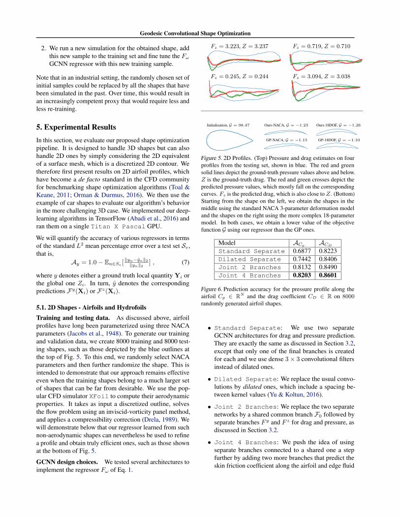
Figure 5. 2D Profiles. (Top) Pressure and drag estimates on fourprofiles from the testing set, shown in blue. The red and greensolid lines depict the ground-truth pressure values above and below.Z is the ground-truth drag. The red and green crosses depict thepredicted pressure values, which mostly fall on the correspondingcurves. Fz is the predicted drag, which is also close to Z. (Bottom)Starting from the shape on the left, we obtain the shapes in themiddle using the standard NACA 3-parameter deformation modeland the shapes on the right using the more complex 18-parametermodel. In both cases, we obtain a lower value of the objectivefunction G using our regressor than the GP ones.

Model ACp ACD

Standard Separate 0.6877 0.8223Dilated Separate 0.7442 0.8406Joint 2 Branches 0.8132 0.8490Joint 4 Branches 0.8203 0.8601

Figure 6. Prediction accuracy for the pressure profile along theairfoil Cp ∈ RN and the drag coefficient CD ∈ R on 8000randomly generated airfoil shapes.

• Standard Separate: We use two separateGCNN architectures for drag and pressure prediction.They are exactly the same as discussed in Section 3.2,except that only one of the final branches is createdfor each and we use dense 3× 3 convolutional filtersinstead of dilated ones.

• Dilated Separate: We replace the usual convo-lutions by dilated ones, which include a spacing be-tween kernel values (Yu & Koltun, 2016).

• Joint 2 Branches: We replace the two separatenetworks by a shared common branch F0 followed byseparate branches F y and F z for drag and pressure, asdiscussed in Section 3.2.

• Joint 4 Branches: We push the idea of usingseparate branches connected to a shared one a stepfurther by adding two more branches that predict theskin friction coefficient along the airfoil and edge fluid


velocity. Although these quantities are not used to com-pute the objective function, the hope is that forcing thenetwork to predict them helps the joint branch to learnthe right features. This is known as disentangling in theComputer Vision literature and has been observed toboost performance (Caruana, 1997; Rifai et al., 2012;Ramsundar et al., 2015).

We report the accuracy results for these four architecturesin Table 6. As observed by Chen et al. (2015) for densesemantic image segmentation, the dilated convolutions per-form better than the standard ones for regression of denseoutputs. Both joint architectures do better than the separateones, with disentangling providing a further performanceboost. At the top of Fig. 5, we superpose the pressure vectorcomputed using the simulator and those predicted by theJoint 4 Branches architecture for 4 different profiles.

Comparing to standard regressors. Since our Joint4 Branches GCNN architecture performs best, we willrefer to it as Ours and we now compare its accuracy to thatof two standard regressors, one based on Gaussian Processes(GPs) and the other on K-Nearest Neighbours (KNNs). ForGPs, we use squared exponential kernels because they haverecently be shown to be effective for aerodynamic predictiontasks (Toal & Keane, 2011; Rosenbaum & Schulz, 2013;Chiplunkar et al., 2017). For KNN regression, we empiri-cally determined that K = 8 combined to a distance-basedneighbor weighting yielded the best results. Note that inorder to compare to such parametric methods, in this experi-ment only, we restrict our training and test set to the NACAparameter space.

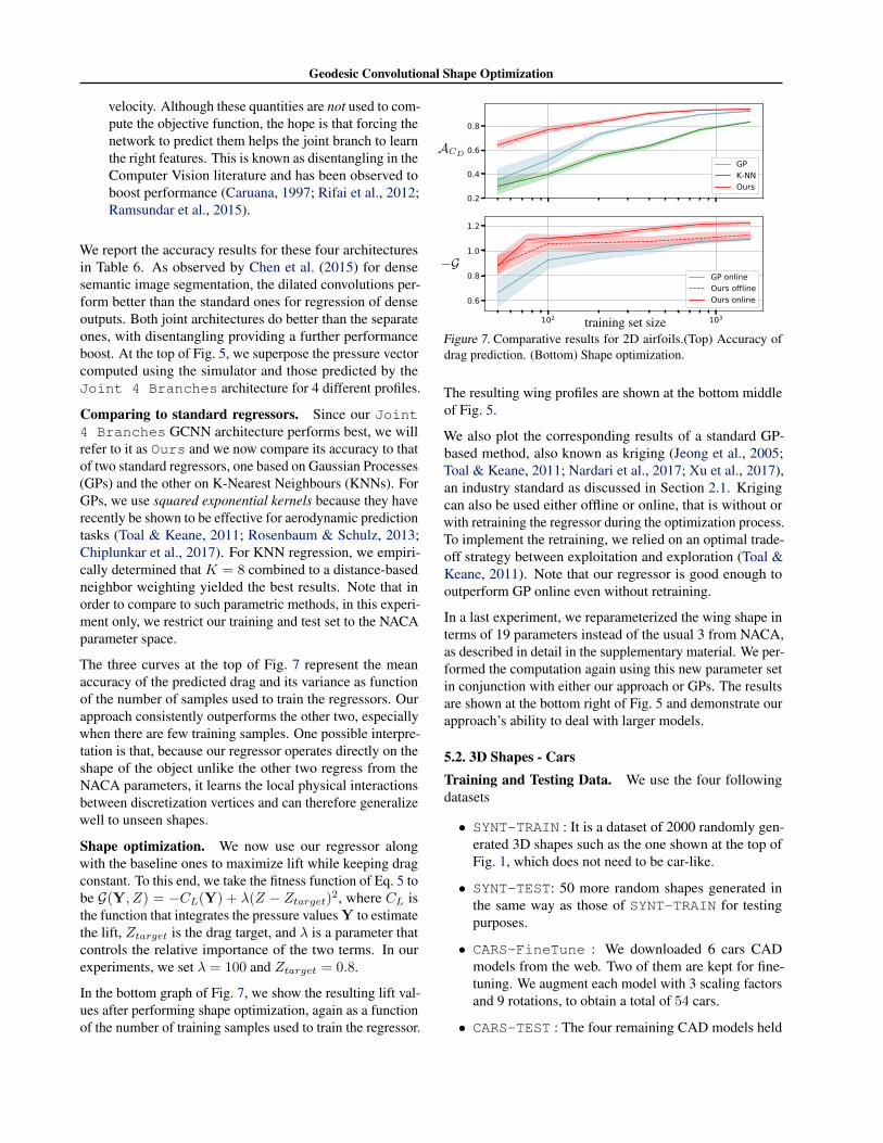
The three curves at the top of Fig. 7 represent the meanaccuracy of the predicted drag and its variance as functionof the number of samples used to train the regressors. Ourapproach consistently outperforms the other two, especiallywhen there are few training samples. One possible interpre-tation is that, because our regressor operates directly on theshape of the object unlike the other two regress from theNACA parameters, it learns the local physical interactionsbetween discretization vertices and can therefore generalizewell to unseen shapes.

Shape optimization. We now use our regressor alongwith the baseline ones to maximize lift while keeping dragconstant. To this end, we take the fitness function of Eq. 5 tobe G(Y, Z) = −CL(Y) + λ(Z − Ztarget)2, where CL isthe function that integrates the pressure values Y to estimatethe lift, Ztarget is the drag target, and λ is a parameter thatcontrols the relative importance of the two terms. In ourexperiments, we set λ = 100 and Ztarget = 0.8.

In the bottom graph of Fig. 7, we show the resulting lift val-ues after performing shape optimization, again as a functionof the number of training samples used to train the regressor.

0.2

0.4

0.6

0.8

GPK-NNOurs

102 103

0.6

0.8

1.0

1.2

GP onlineOurs offlineOurs online

−G

ACD

training set sizeFigure 7. Comparative results for 2D airfoils.(Top) Accuracy ofdrag prediction. (Bottom) Shape optimization.

The resulting wing profiles are shown at the bottom middleof Fig. 5.

We also plot the corresponding results of a standard GP-based method, also known as kriging (Jeong et al., 2005;Toal & Keane, 2011; Nardari et al., 2017; Xu et al., 2017),an industry standard as discussed in Section 2.1. Krigingcan also be used either offline or online, that is without orwith retraining the regressor during the optimization process.To implement the retraining, we relied on an optimal trade-off strategy between exploitation and exploration (Toal &Keane, 2011). Note that our regressor is good enough tooutperform GP online even without retraining.

In a last experiment, we reparameterized the wing shape interms of 19 parameters instead of the usual 3 from NACA,as described in detail in the supplementary material. We per-formed the computation again using this new parameter setin conjunction with either our approach or GPs. The resultsare shown at the bottom right of Fig. 5 and demonstrate ourapproach’s ability to deal with larger models.

5.2. 3D Shapes - CarsTraining and Testing Data. We use the four followingdatasets

• SYNT-TRAIN : It is a dataset of 2000 randomly gen-erated 3D shapes such as the one shown at the top ofFig. 1, which does not need to be car-like.

• SYNT-TEST: 50 more random shapes generated inthe same way as those of SYNT-TRAIN for testingpurposes.

• CARS-FineTune : We downloaded 6 cars CADmodels from the web. Two of them are kept for fine-tuning. We augment each model with 3 scaling factorsand 9 rotations, to obtain a total of 54 cars.

• CARS-TEST : The four remaining CAD models held


out for final testing, yielding a total of 108 shapes afteraugmentation.

To generate our random shapes, we introduce a functionfC : R3 → R3, where C represents the parameters thatcontrol its behavior and apply it to an initially spherical setof vertices X0. f is an algebraic function that applies ro-tations, translations, affine transformations, and dilatationswith respect to the center of the shape, which lets us createa wide variety of shapes. The shape at the top Fig. 1 is oneof them and we provide more in the supplementary material.We give the precise definition of f in the supplementarymaterial and take C to be a 21D vector. We used the in-dustry standard Ansys Fluent (Inc., 2011) to computetheir aerodynamic properties with the k-epsilon turbulencemodel.

VALID TEST TEST-FTMethod ACD

ACDACD

CNN 70.1 % 38.4% 58.1%Ours 77.2% 51.5 % 70.3%

Figure 8. Regression results on our three 3D test sets.

Comparing to Standard Regressors. In Fig. 8, we re-port the accuracy of our regressor under three different train-ing and testing scenarios:

• VALID : The regressor is first trained onSYNT-TRAIN and tested on SYNT-TEST. Thisis a sanity check since testing is carried out on shapesthat have the same statistical distribution as the trainingones.

• TEST : The regressor is trained on SYNT-TRAIN andtested on CARS-TEST. This is much more challengingsince the testing shapes are those of real cars while thetraining ones are not.

• TEST-FT : The regressor is trained on SYNT-TRAIN,fine tuned using CARS-FineTune, and tested onCARS-TEST. This is similar to TEST but we helpthe regressor by giving it a few real car shapes makinga few additional epochs of training.

Unsurprisingly, the accuracy on TEST is lower than onVALID. Nevertheless, fine-tuning with a few car-like exam-ples brings it back up. To assess the importance of usingGCNNs instead of regular CNNs, we re-ran all three scenar-ios using a standard CNN of similar complexity. In otherterms, we keep the same architecture where the geodesicconvolutions of Eqs. 3 and 4, are replaced by standard ones.As can be seen on the top row of the figure, the accuracynumbers are much worse in all three cases.

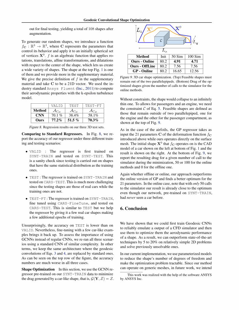
Shape Optimization In this section, we use the GCNN re-gressor pre-trained on our SYNT-TRAIN data to minimizethe drag generated by a car-like shape, that is, G(Y, Z) = Z.

Method Init 50 Sim 100 SimOurs - Online 80.2 4.91 4.71Ours - OffLine 80.2 7.56 7.56

GP - Online 80.2 16.65 12.56

Figure 9. 3D car shape optimization. (Top) Feasible shapes mustremain out of the two parallelepipeds. (Bottom) Drag of the op-timized shapes given the number of calls to the simulator for theonline methods.

Without constraints, the shape would collapse to an infinitelythin one. To allows for passengers and an engine, we needthe constraint C of Eq. 5. Feasible shapes are defined asthose that remain outside of two parallelepiped, one forthe engine and the other for the passenger compartment, asshown at the top of Fig. 9.

As in the case of the airfoils, the GP regressor takes asinput the 21 parameters C of the deformation function fCintroduced above while ours operates directly on the surfacemesh. The initial shape X0 that fC operates on is the CADmodel of a car shown on the left at bottom of Fig. 1 and theresult is shown on the right. At the bottom of Fig. 9, wereport the resulting drag for a given number of call to thesimulator during the minimization, 50 or 100 for the onlinemethods and 0 for the offline one.

Again whether offline or online, our approach outperformsthe online version of GP and finds a better optimum for the21 parameters. In the online case, note that with only 50 callsto the simulator our result is already close to the optimumeven though our network, pre-trained on SYNT-TRAIN,had never seen a car before.

6. Conclusion

We have shown that we could first train Geodesic CNNsto reliably emulate a output of a CFD simulator and thenuse them to optimize them the aerodynamic performanceof a shape. As a result, we can outperform state-of-the-arttechniques by 5 to 20% on relatively simple 2D problemsand solve previously unsolvable ones.

In our current implementation, we use parameterized modelsto reduce the shape’s number of degrees of freedom andmake the optimization problem tractable. Since our methodcan operate on generic meshes, in future work, we intend

This work was realized with the help of the software ANSYSby ANSYS Inc.


to use the Laplacian parameterization introduced by Ngoet al. (2016) to increase or decrease the number of degreesof freedom at will and make our approach fully flexible.

ReferencesAbadi, Martın, Barham, Paul, Chen, Jianmin, Chen, Zhifeng,

Davis, Andy, Dean, Jeffrey, Devin, Matthieu, Ghemawat,Sanjay, Irving, Geoffrey, Isard, Michael, Kudlur, Man-junath, Levenberg, Josh, Monga, Rajat, Moore, Sherry,Murray, Derek G., Steiner, Benoit, Tucker, Paul, Vasude-van, Vijay, Warden, Pete, Wicke, Martin, Yu, Yuan, andZheng, Xiaoqiang. Tensorflow: A system for large-scalemachine learning. In USENIX Conference on OperatingSystems Design and Implementation, pp. 265–283, 2016.

Alexandersen, J., Sigmund, O., and Aage, N. Large ScaleThree-Dimensional Topology Optimization of Heat SinksCooled by Natural Convection. International Journal ofHeat and Mass Transfer, 100(Supplement C):876 – 891,2016. ISSN 0017-9310.

Allaire, G. A Review of Adjoint Methods for SensitivityAnalysis, Uncertainty Quantification and Optimizationin Numerical Codes. Ingenieurs de l’Automobile, 836:33–36, July 2015.

Bengio, Y., Delalleau, O., and Roux, N. Le. The Curse ofHighly Variable Functions for Local Kernel Machines. InAdvances in Neural Information Processing Systems, pp.107–114, 2006.

Bommes, D., Lvy, B., Pietroni, N., Puppo, E., a, C. Silv,Tarini, M., and Zorin, D. State of the art in quad meshing.In Eurographics STARS, 2012.

Bommes, David, Levy, Bruno, Pietroni, Nico, Puppo, En-rico, Silva, Claudio, Tarini, Marco, and Zorin, Denis.Quad-mesh generation and processing: A survey. Com-put. Graph. Forum, 32(6):51–76, September 2013. ISSN0167-7055. doi: 10.1111/cgf.12014.

Caruana, R. Multitask Learning. Machine Learning, 28,1997.

Chen, L.-C., Papandreou, G., Kokkinos, I., Murphy, K.,and Yuille, A. Semantic Image Segmentation with DeepConvolutional Nets and Fully Connected CRFs. In Inter-national Conference for Learning Representations, 2015.

Chiplunkar, Ankit, Bosco, Elisa, and Morlier, Joseph. Gaus-sian process for aerodynamic pressures prediction in fastfluid structure interaction simulations. In World Congressof Structural and Multidisciplinary Optimisation, pp. 221–233. Springer, 2017.

Drela, M. XFOIL: An Analysis and Design System forLow Reynolds Number Airfoils. In Conference on LowReynolds Number Aerodynamics, pp. 1–12, Berlin, Hei-delberg, 1989. Springer Berlin Heidelberg.

Gao, Yisheng, Wu, Yizhao, and Xia, Jian. Automatic Dif-ferentiation Dased Discrete Adjoint Method for Aero-dynamic Design Optimization on Unstructured Meshes.Chinese Journal of Aeronautics, 30(2):611 – 627, 2017.

Gholizadeh, S. and Seyedpoor, S.M. Shape Optimizationof Arch Dams by Metaheuristics and Neural Networksfor Frequency Constraints . Scientia Iranica, 18(5):1020– 1027, 2011.

Gosselin, L., Tye-Gingras, M., and Mathieu-Potvin, F. Re-view of Utilization of Genetic Algorithms in Heat Trans-fer Problems. International Journal of Heat and MassTransfer, 52(9):2169 – 2188, 2009.

Gregson, James, Sheffer, Alla, and Zhang, Eugene. All-hexmesh generation via volumetric polycube deformation.In Computer graphics forum, volume 30, pp. 1407–1416.Wiley Online Library, 2011.

Guo, X., Li, W., and Iorio, F. Convolutional Neural Net-works for Steady Flow Approximation. In Conference onKnowledge Discovery and Data Mining, 2016.

He, K., Zhang, X., Ren, S., and Sun, J. Deep residual learn-ing for image recognition. In Conference on ComputerVision and Pattern Recognition, pp. 770–778, 2016.

Inc., Ansys. ANSYS FLUENT Theory Guide. November2011.

Jacobs, Eastmann N., Ward, Kenneth E., and Pinkerton,Robert M. The characteristics of 78 related airfoil sec-tions from tests in the variable density wind tunnel. Tech-nical Report 460, 1948.

Jeong, Shinkyu, Murayama, Mitsuhiro, and Yamamoto,Kazuomi. Efficient optimization design method usingkriging model. Journal of Aircraft, 42(2):413–420, 2005.

Kingma, D.P. and Ba, J. Adam: A Method for StochasticOptimisation. In International Conference for LearningRepresentations, 2015.

Kipf, Thomas N and Welling, Max. Semi-supervised clas-sification with graph convolutional networks. arXivpreprint arXiv:1609.02907, 2016.

Lundberg, A., Hamlin, P., Shankar, D., Broniewicz, A.,Walker, T., and Landstram, C. Automated AerodynamicVehicle Shape Optimization Using Neural Networks andEvolutionary Optimization. SAE International Journal ofPassenger Cars - Mechanical Systems, 8:242–251, April2015.


McNamara, G. and Zanetti, G. Use of the Boltzmann Equa-tion to Simulate Lattice-gas Automata. Physical ReviewLetters, 61(20):2332, 1988.

Monti, Federico, Boscaini, Davide, Masci, Jonathan,Rodola, Emanuele, Svoboda, Jan, and Bronstein,Michael M. Geometric deep learning on graphs andmanifolds using mixture model cnns. arXiv preprintarXiv:1611.08402, 2016.

Nardari, C., Mann, A., and Schindele, T. Characterizationof the effects of manufacturing geometry details on ex-haust flow noise using lattice boltzmann based methodsimulations. 2017.

Ngo, D., Ostlund, J., and Fua, P. Template-Based Monocu-lar 3D Shape Recovery Using Laplacian Meshes. IEEETransactions on Pattern Analysis and Machine Intelli-gence, 38(1):172–187, 2016.

Orman, E. and Durmus, G. Comparison of Shape Optimiza-tion Techniques Coupled with Genetic Algorithms for aWind Turbine Airfoil. In IEEE Aerospace Conference,pp. 1–7, March 2016.

Preen, R. J. and Bull, L. Toward the Coevolution of NovelVertical-Axis Wind Turbines. IEEE Transactions on Evo-lutionary Computation, 2:284–293, 2015.

Quarteroni, A. and Quarteroni, S. Numerical Models forDifferential Problems, volume 2. Springer, 2009.

Ramsundar, Bharath, Kearnes, Steven M., Riley, Patrick,Webster, Dale, Konerding, David E., and Pande, Vijay S.Massively multitask networks for drug discovery. CoRR,abs/1502.02072, 2015.

Rasmussen, C. E. and Williams, C. K. Gaussian Processfor Machine Learning. MIT Press, 2006.

Rifai, Salah, Bengio, Yoshua, Courville, Aaron, Vincent,Pascal, and Mirza, Mehdi. Disentangling factors of vari-ation for facial expression recognition. In Fitzgibbon,Andrew, Lazebnik, Svetlana, Perona, Pietro, Sato, Yoichi,and Schmid, Cordelia (eds.), Computer Vision – ECCV2012, pp. 808–822, Berlin, Heidelberg, 2012. SpringerBerlin Heidelberg.

Rosenbaum, Benjamin and Schulz, Volker. Response sur-face methods for efficient aerodynamic surrogate models.In Computational Flight Testing, pp. 113–129. Springer,2013.

Skinner, S.N. and Zare-Behtash, H. State-of-the-art in aero-dynamic shape optimisation methods. Applied Soft Com-puting, 62(Supplement C):933 – 962, 2018. ISSN 1568-4946.

Tarini, M., Hormann, K., Cignoni, P., and Montani, C.Polycube-maps. ACM Transactions on Graphics, 23(3):853–860, 2004.

Toal, David JJ and Keane, Andy J. Efficient multipointaerodynamic design optimization via cokriging. Journalof Aircraft, 48(5):1685–1695, 2011.

Tompson, J., Schlachter, K., Sprechmann, P., and Perlin, K.Accelerating Eulerian Fluid Simulation With Convolu-tional Networks. ArXiv e-prints, July 2016.

Ulaganathan, S. and Asproulis, N. Surrogate Models forAerodynamic Shape Optimization, pp. 285–312. Springer,2013.

Xian, W. and Takayuki, A. Multi-GPU Performance ofIncompressible Flow Computation by Lattice BoltzmannMethod on GPU Cluster. Parallel Computing, 37(9):521–535, 2011.

Xu, Gang, Liang, Xifeng, Yao, Shuanbao, Chen, Dawei, andLi, Zhiwei. Multi-objective aerodynamic optimization ofthe streamlined shape of high-speed trains based on thekriging model. PLOS ONE, 12(1):1–14, 01 2017.

Yu, F. and Koltun, V. Multi-Scale Context Aggregation byDilated Convolutions. In ICLR, 2016.

7. AppendixIn this supplementary material, we first provide additionaldetail on the handling of the irregular vertices of the Cube-Mesh CNNs of Section 3.1. We then give analytical defi-nitions of the 2D and 3D deformation parameterizations ofSections 5.1 and 5.2.

7.1. Handling Singular Points for Semi-RegularQuad-Meshes

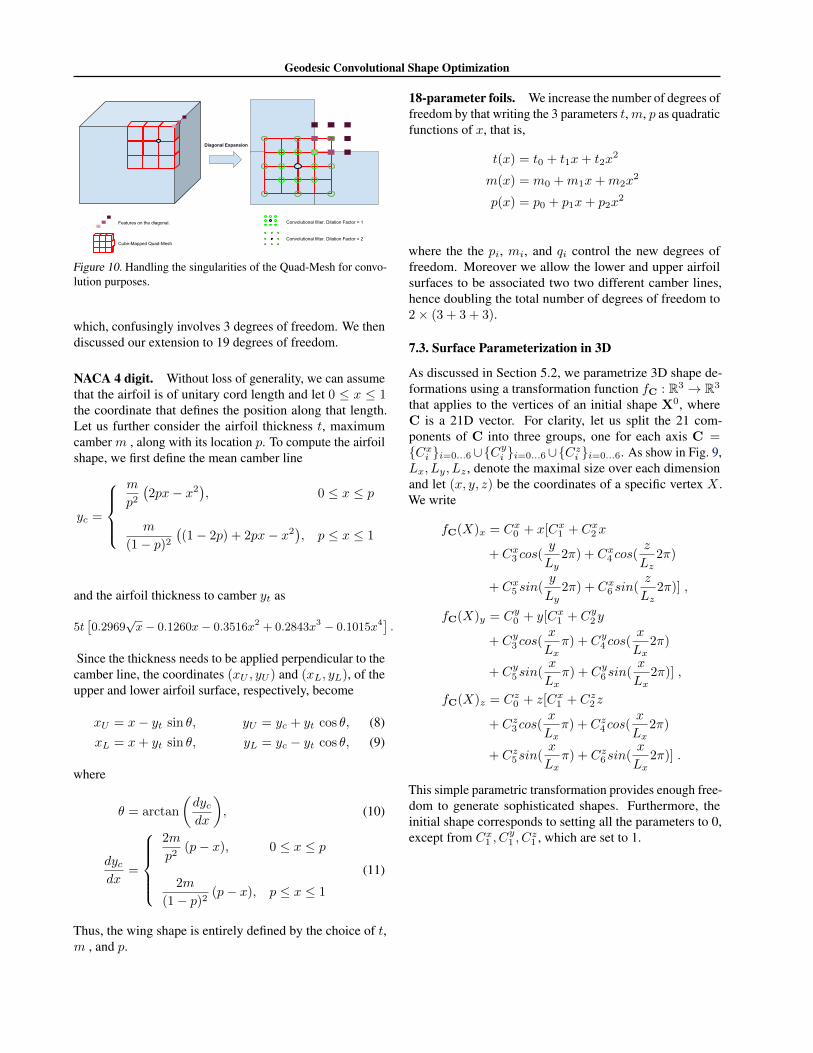
As discussed in Section 3.1 of the paper, when mapping asurface onto a cube-mesh, we have to deal with irregular ver-tices, which correspond to the corners of the cube and havethree neighbors instead of four. To perform convolutionsefficiently we first unfold the cube surface onto a plane. Asillustrated by Fig. 10, we can then simply pad irregular cor-ners with the feature values associated to cube edges. Thisenables us to use standard convolutional kernels even inthe neighborhood of irregular vertices. Furthermore, sincewe use Geodesic Convolutions, the irregularity is naturallyhandled by the interpolation operation.

7.2. Airfoil Parameterization in 2D

In this section we will first briefly describe the standardNACA airfoil 4 digit parameterization (Jacobs et al., 1948),


Features on the diagonal.

Convolutional filter. Dilation Factor = 2

Convolutional filter. Dilation Factor = 1

Cube-Mapped Quad-Mesh

Diagonal Expansion

Figure 10. Handling the singularities of the Quad-Mesh for convo-lution purposes.

which, confusingly involves 3 degrees of freedom. We thendiscussed our extension to 19 degrees of freedom.

NACA 4 digit. Without loss of generality, we can assumethat the airfoil is of unitary cord length and let 0 ≤ x ≤ 1the coordinate that defines the position along that length.Let us further consider the airfoil thickness t, maximumcamber m , along with its location p. To compute the airfoilshape, we first define the mean camber line

yc =

m

p2(2px− x2

), 0 ≤ x ≤ p

m

(1− p)2((1− 2p) + 2px− x2

), p ≤ x ≤ 1

and the airfoil thickness to camber yt as

5t[0.2969

√x− 0.1260x− 0.3516x2 + 0.2843x3 − 0.1015x4] .

Since the thickness needs to be applied perpendicular to thecamber line, the coordinates (xU , yU ) and (xL, yL), of theupper and lower airfoil surface, respectively, become

xU = x− yt sin θ, yU = yc + yt cos θ, (8)xL = x+ yt sin θ, yL = yc − yt cos θ, (9)

where

θ = arctan

(dycdx

), (10)

dycdx

=

2m

p2(p− x), 0 ≤ x ≤ p

2m

(1− p)2 (p− x), p ≤ x ≤ 1

(11)

Thus, the wing shape is entirely defined by the choice of t,m , and p.

18-parameter foils. We increase the number of degrees offreedom by that writing the 3 parameters t,m, p as quadraticfunctions of x, that is,

t(x) = t0 + t1x+ t2x2

m(x) = m0 +m1x+m2x2

p(x) = p0 + p1x+ p2x2

where the the pi, mi, and qi control the new degrees offreedom. Moreover we allow the lower and upper airfoilsurfaces to be associated two two different camber lines,hence doubling the total number of degrees of freedom to2× (3 + 3 + 3).

7.3. Surface Parameterization in 3D

As discussed in Section 5.2, we parametrize 3D shape de-formations using a transformation function fC : R3 → R3

that applies to the vertices of an initial shape X0, whereC is a 21D vector. For clarity, let us split the 21 com-ponents of C into three groups, one for each axis C ={Cxi }i=0...6∪{Cyi }i=0...6∪{Czi }i=0...6. As show in Fig. 9,Lx, Ly, Lz , denote the maximal size over each dimensionand let (x, y, z) be the coordinates of a specific vertex X .We write

fC(X)x = Cx0 + x[Cx1 + Cx2 x

+ Cx3 cos(y

Ly2π) + Cx4 cos(

z

Lz2π)

+ Cx5 sin(y

Ly2π) + Cx6 sin(

z

Lz2π)] ,

fC(X)y = Cy0 + y[Cx1 + Cy2 y

+ Cy3 cos(x

Lxπ) + Cy4 cos(

x

Lx2π)

+ Cy5 sin(x

Lxπ) + Cy6 sin(

x

Lx2π)] ,

fC(X)z = Cz0 + z[Cx1 + Cz2z

+ Cz3 cos(x

Lxπ) + Cz4 cos(

x

Lx2π)

+ Cz5sin(x

Lxπ) + Cz6sin(

x

Lx2π)] .

This simple parametric transformation provides enough free-dom to generate sophisticated shapes. Furthermore, theinitial shape corresponds to setting all the parameters to 0,except from Cx1 , C

y1 , C

z1 , which are set to 1.

Documents

Geodesic Convolutional Shape Optimization