SMAPRadiometer-OnlyTropicalCycloneSizeandStrengthAlexanderFore,SimonYueh,Wenqing

Tang,BryanSCles,AkikoHayashiJetPropulsionLaboratory,California

InsCtuteofTechnology

©2018CaliforniaInsCtuteofTechnology,GovernmentSponsorshipacknowledged

SMAPOverview

Partners • JPL (project & payload management, science, spacecraft, radar, mission operations, science processing)

• GSFC (science, radiometer, science processing) Launch • January 31, 2015 on Delta 7320-10C Launch System Orbit • Polar Sun-synchronous; 685 km altitude Duration • 3 years Payload • L-band (non-imaging) synthetic aperture radar (JPL)

• L-band radiometer (GSFC) • Shared 6-m rotating (13 to 14.6 rpm) antenna (JPL)

PrimaryScienceObjec/ves•  Global,high-resoluConmappingofsoilmoistureanditsfreeze/

thawstateto•  Linkterrestrialwater,energy,andcarbon-cycleprocesses•  EsCmateglobalwaterandenergyfluxesatthelandsurface•  QuanCfynetcarbonfluxinboreallandscapes•  Extendweatherandclimateforecastskill•  DevelopimprovedfloodanddroughtpredicConcapability

MissionImplementa/on

h"p://smap.jpl.nasa.gov/

NRCEarthScienceDecadalSurvey(2007)recommendedSMAPasaTier1mission

6mantennaRadiometerresoluCon:40km

01:00 02:00 03:00 04:00 05:00 06:000

12.5

25

37.5

50

62.5

75

87.5

100W

ind

Spee

d [m

/s]

SFMR vs SMAP for Ignacio at 2015−08−30 03:53:05

0

12.5

25

37.5

50

62.5

75

87.5

100

Rai

n R

ate

[mm

/hr]

SFMR SPD 5kmSFMR SPD 40 kmSMAP SPDSFMR RR 5 kmSFMR RR 40 km

SFMR vs SMAP for Ignacio at 2015−08−30 03:53:05

−151 −150 −149 −148 −147 −146 −145 −14413

14

15

16

17

18

19

20

0

5

10

15

20

25

30

35

40

SFMRMatchupsfor2015-2017SFMR>20m/s SFMR>25m/s

DTime Counts Bias STD Corr Counts Bias STD Corr

15 43 0.88 3.10 0.85 18 0.66 3.82 0.85

30 79 1.61 3.54 0.81 38 1.69 3.99 0.77

45 116 1.51 3.54 0.80 58 1.59 4.05 0.73

90 261 1.15 3.15 0.84 102 1.90 3.80 0.73

180 523 1.21 3.23 0.81 196 1.93 3.97 0.69

240 632 0.90 3.33 0.79 245 1.31 4.23 0.63

300 791 0.58 3.66 0.74 316 0.52 4.66 0.58

360 954 0.20 3.96 0.73 363 0.38 4.63 0.60

•  AverageSFMRalong-trackto60km,pickpointofnearestapproachtoSMAPcell.

•  Usebest-tracktoshicSFMRtrackstoSMAPobservaConCme.

15 20 25 30 35 40 45 50 55 6015

20

25

30

35

40

45

50

55

60

SFMR Wind Speed [m/s]

SM

AP

Win

d S

peed [m

/s]

SMAP vs SFMR; Best Fit Slope: 0.96; Corr: 0.81Mean Pct Error > 15 m/s: 15

SMAPBest Fit1:1

360minmatchupCme

SMAPWindRadii•  WevalidateagainsttheATCFB-deckdatasets.•  ForeachSMAPcyclonehit:–  Computecontoursat(34,50,64)knotwindthresholds.

–  Extractlongestcontourineachcompassquadrantandcomputethe90%thresholdvalue.

0 50 100 150 2000

20

40

60

80

100

120

140

160

180

200

NHC Wind Radii [km]

SM

AP

Win

d R

ad

ii [k

m]

SMAP wind radii versus NHC wind radii

34kt50kt64kt

−200 −150 −100 −50 0 50 100 150 2000

10

20

30

40

50

60

70

80

90

100

110

SMAP RXX − NHC RXX [km]

Counts

SMAP wind radii versus NHC wind radii

34 kt; Median: −0.04; CDF68: 42.14; CORR: 0.8650 kt; Median: 1.63; CDF68: 24.99; CORR: 0.6564 kt; Median: 8.96; CDF68: 21.63; CORR: 0.64

WindRadiiResults

•  SMAPwindradiiareinreasonableagreementwithATCFB-deckradii:– ATCFwindradiiesCmateshave~20-40%error.– GoodcorrelaContoATCFradii.– SMAPrelaCvelyunbiased.

Summary•  UsingSFMRwefindgoodagreementtoabout40ms-1

–  PosiCvebiasbetween30-40ms-1nolargerthan3ms-1–  OverallSTDascomparedtoSFMRisontheorderof4ms-1forwindspeeds

largerthan25ms-1

•  ComparisonstoATCFB-deckdatasetsshowsSMAPprovidesreasonablyunbiasedsizeesCmateswithgoodcorrelaContoATCFvalues.

•  Overall,SMAPcanprovidevaluableinformaCononTropicalCyclonesizeandaveragedintensity.

•  Peer-reviewedpublicaCons:–  S.H.Yuehetal.,"SMAPL-BandPassiveMicrowaveObservaConsofOcean

SurfaceWindDuringSevereStorms,"inIEEETransacConsonGeoscienceandRemoteSensing,vol.54,no.12,pp.7339-7350,Dec.2016.

–  A.G.Fore,etal.,"CombinedAcCve/PassiveRetrievalsofOceanVectorWindandSeaSurfaceSalinityWithSMAP,"inIEEETransacConsonGeoscienceandRemoteSensing,vol.54,no.12,pp.7396-7404,Dec.2016.

–  N.Reul,etal.,“AnewgenerateofTropicalCycloneSizemeasurementsfromspace,”inBAMS,Earlyrelease(online).10.1175/BAMS-D-15-00291.1

16:30 17:00 17:30 18:00 18:30 19:00 19:300

12.5

25

37.5

50

62.5

75

87.5

100W

ind

Spee

d [m

/s]

SFMR vs SMAP for PATRICIA at 2015−10−23 13:10:13

0

6.25

12.5

18.75

25

31.25

37.5

43.75

50

Rai

n R

ate

[mm

/hr]

SFMR SPD 5kmSFMR SPD 40 kmSMAP SPDSFMR RR 5 kmSFMR RR 40 km

SFMR vs SMAP for PATRICIA at 2015−10−23 13:10:13

−109 −108 −107 −106 −105 −104 −103 −102

14

15

16

17

18

19

20

21

0

10

20

30

40

50

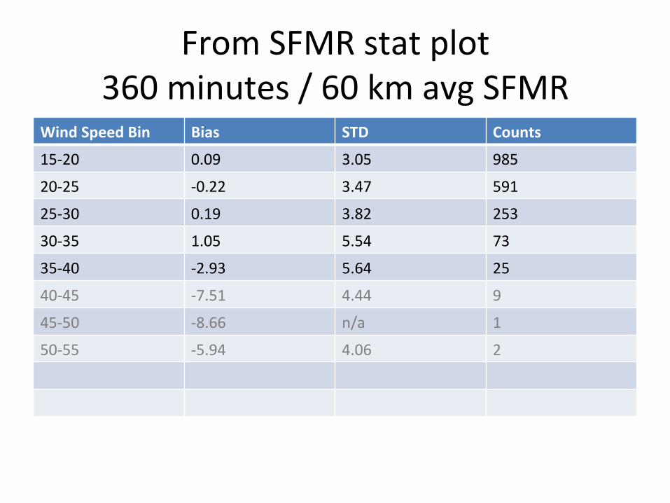
FromSFMRstatplot360minutes/60kmavgSFMR

WindSpeedBin Bias STD Counts

15-20 0.09 3.05 985

20-25 -0.22 3.47 591

25-30 0.19 3.82 253

30-35 1.05 5.54 73

35-40 -2.93 5.64 25

40-45 -7.51 4.44 9

45-50 -8.66 n/a 1

50-55 -5.94 4.06 2

60km

SFMRTrack

ClosestpointsofapproachtoSWCcenter

ShicSFMRtracksusingbest-track(Cme,locaCon)toSMAPCmeIdenCfyclosestpointsofapproachtoSWC;maybemulCpleForeachclosestpointofapproach:AverageSFMRalong-trackto60kmcenteredonthatpointKeepifcloserthan12.5kmandCmeoffsetlessthan360min

25kmSWCspacing

SMAPSWCs

60km

0 2.5 5 7.5 10 12.5 15 17.5 20 22.5 25 27.5 30 32.5 35−2

−1

0

1

2

3

4

5

6

7

8

9

10

Mean of SMAP/RapidScat Wind Speed [m/s]

Spee

d Er

ror [

m/s

]

SMAP/RapidScat Wind Speed MatchupsWindSat / SSMI/S indicate no−rain; Within: 30 minutes

Speed BiasSpeed STD

RapidScat Wind Speed [m/s]

SMAP

Win

d Sp

eed

[m/s

]

2D Histogram of SMAP/RS wind Speeds [dB Counts]Within: 30 minutes; 3705445 total

0 2.5 5 7.5 10 12.5 15 17.5 20 22.5 25 27.5 30 32.5 350

2.55

7.510

12.515

17.520

22.525

27.530

32.535

0

5

10

15

20

25

30

35

40

45

50

SMAP/RapidScat/WindSatcollocaCons(30m)•  OnlyextractjointcollocaConswithin30minutesofSMAP.

–  3.7millionmatchups.•  UseWindSattoremoverainyobservaCons.•  Findnearlyzerospeedbiasupto26m/s,notenoughdatapast

that.•  2dhistogramdoesnotshowanytrendofincreasingSMAPspeed

biasascomparedtoRapidScat

0 2.5 5 7.5 10 12.5 15 17.5 20 22.5 25 27.5 30 32.5 35−2

−1

0

1

2

3

4

5

6

7

8

9

10

Mean of SMAP/RapidScat Wind Speed [m/s]

Spee

d Er

ror [

m/s

]

SMAP/RapidScat Wind Speed MatchupsWindSat / SSMI/S indicate no−rain; Within: 90 minutes

Speed BiasSpeed STD

RapidScat Wind Speed [m/s]

SMAP

Win

d Sp

eed

[m/s

]

2D Histogram of SMAP/RS wind Speeds [dB Counts]Within: 90 minutes; 13306873 total

0 2.5 5 7.5 10 12.5 15 17.5 20 22.5 25 27.5 30 32.5 350

2.55

7.510

12.515

17.520

22.525

27.530

32.535

0

5

10

15

20

25

30

35

40

45

50

SMAP/RapidScat/WindSatcollocaCons(90m)•  Sameaspreviouswith90minutecollocaConCme.–  13millionmatchups.

•  Findverysmallspeedbiasupto30m/s(order1m/s).•  2dhistogramshowdatadistributednear1:1line,noevidenceoflargeposiCveSMAPbiasnear30m/sascomparedtoRapidScat.

0 10 20 30 40 50−10

−8

−6

−4

−2

0

2

4

6

8

10

Averaged SFMR Rain Rate [mm/hr]SMAP

TB

Win

d Sp

eed −

Aver

aged

SFM

R W

ind

Spee

d [m

/s]

Wind Speed bias versus SFMR rain rate (SFMR spd > 20 m/s)

SFMR60kmaverageSFMR>20m/sMatch-upCmewithin360min

Insufficientdata

4

j-1

j

j+1

i-1 i i+1

Fig. 3. An example of the L2A gridding algorithm: the solid black grid lines represent the boundaries between the SWCs while the two ellipses

represent two sequential L1B footprint observations. i represents the cross-track coordinate while j represents the along-track coordinate. The

dashed boxes within each SWC indicate the size of the “overlap” region. Any L1B observation whose footprint falls within the dashed “overlap”

region for each SWC will be included in that SWC for salinity processing. For example, the dark gray footprint will be assigned to SWCs

{(i, j � 1) , (i, j) , (i+ 1, j � 1) , (i+ 1, j)}.

“latitudes” are linearly scaled to generate the Salinity Wind Cell (SWC) grid indices which are approximately 25

km in spacing [6].

After computing the SOM coordinates for all TB footprints, we assign each TB footprint to every SWC that

the footprint 3 dB contour overlaps a configurable portion of. This gridding algorithm was developed for Version

3 of the QuikSCAT data products and is currently used for processing RapidScat data [7], and is known as the

overlap method. This gridding algorithm over-samples the TB observations onto the SWC swath in a way that is

consistent with the measurement geometry. In Figure 3 we have an example of the L2A gridding algorithm. In this

figure the solid black lines represent the boundaries of the SWCs while the dashed lines indicate the size of the

“overlap” region, which is set to 0.75 the size of the SWC. Any L1B TB observation whose footprint falls within

the dashed “overlap” region for each SWC will be included in that SWC for salinity processing. For example, the

dark gray footprint will be assigned to SWCs {(i, j � 1) , (i, j) , (i+ 1, j � 1) , (i+ 1, j)}. The data are posted at

approximately 25 km, however, the intrinsic resolution of the L2A data is somewhat larger than the resolution of

the L1B footprints which is 40 km.

After assigning every L1B TB observation to SWCs we apply land and ice flagging to the individual TB

measurements and remove all observations that are flagged as land/ice from each SWC. Any SWC containing an

observation that is flagged as land/ice and was removed is then flagged as having possible land/ice contamination

in the quality flag. We then average the H-pol and V-pol TB for fore and aft looks separately to obtain up to four

looks for each SWC. We refer to these four looks as “flavors” of TB (fore H-pol, aft H-pol, fore V-pol, aft V-pol).

The reason we must aggregate the fore and aft looks separately is that the wind directional response is a function

March 15, 2016 DRAFT

15 20 25 30 35 40 45 50 55 600

2

4

6

8

10

12

14

16

18

20

Cross Track Index

Mea

n N

umbe

r of L

1B T

Bs p

er S

WC

Mean Number of L1B TBs per look in a SWC

H/ForeH/AftV/ForeV/Aft

15 20 25 30 35 40 45 50 55 600.1

0.2

0.3

0.4

0.5

0.6

0.7

0.8

Cross Track Index

Aggr

egat

e N

EDT

By F

lavo

r

Aggregate NEDT By Flavor

H/ForeH/AftV/ForeV/Aft

L2AGridding

25km